a sensitivity analysis of central station flat-plate ... anal... · agreement de-ai01-76et20356...
TRANSCRIPT
5101-265Flat-PlateSolar Array Project
DOE/JPL-1012-114
Distribution Category UC-63b
f
A Sensitivity Analysis ofCentral Station Flat-PlatePhotovoltaic Systems and Implicationsfor National Photovoltaics ProgramPlanningM.R. CrosettiB.L. JacksonR.W. Aster
r2f«
KO
«?FEBJ986
001
§?^STl FACILITY ^
(NASA-Cfi-1765264 ^£/nc\7S3^
^^pE-SH'-sHC AOVflf A01 f ropuls icn lab.) 65 p
August 30, 1985
Prepared forU.S. Department of EnergyThrough an Agreement withNational Aeronautics and Space AdministrationbyJet Propulsbn LaboratoryCalifornia Institute of TechnologyPasadena, California
JPL Publication 85-92

TECHNICAL REPORT STANDARD TITLE PAGE
1. Report No. 85-92 2. Government Accession No.
4. Tit le and Subtitle A Sensitivity Analysis of CentralFlat-Plate Photovoltaic Systems and Implications foiNational Photovoltaics Program Planning
7. Author(s)M. R. Crosetti
9. Performing Organization Name or
JET PROPULSION LABCCalifornia Institul4800 Oak Grove DriiPasadena, Calif orn:
id Address
DRATORY:e of Technology/eLa 91109
12. Sponsoring Agency Name and Address
NATIONAL AERONAUTICS AND SPACE ADMINISTRATIONWashington, D.C. 20546
3. Recipient's Catalog No.
5. Report DateAueust 30. 1985
6. Performing Organization Code
8. Performing Organization Report No.
10. Work Unit No.
11. Contract or Grant No.NAS7-918
13. Type of Report and Period Covered
JPL Publication
14. Sponsoring Agency Code
15. Supplementary Notes Sponsored by the U.S. Department of Energy through InteragencyAgreement DE-AI01-76ET20356 with NASA; also identified as DOE/JPL-1012-114 and asJPL Project No. 5101-265 (RTOP or Customer Code 776-52-61).
16. Abstract
The purpose of this study is to explore the sensitivity of the NationalPhotovoltaic Research Program goals to changes in individual photovoltaicsystem parameters. Using the relationship between lifetime cost and systemperformance parameters, tests were made to see how overall photovoltaic systemenergy costs are affected by changes in the goals set for module cost andefficiency, system component costs and efficiencies, operation and maintenancecosts, and indirect costs. The results are presented in tables and figuresfor easy reference.
17. Key Words (Selected by Author(s))
Power SourcesCrystallographySolid-state physics
18. Distribution Statement
Unclassified-unlimited
19. Security Clossif. (of this report)
Unclassified
20. Security Clossif. (of this page)
Unclassified
21. No. of Poges
68
22. Price
JPL 01B4 R9I83

5101-265Flat-PlateSolar Array Project
DOE/JPL-1012-114
Distribution Category UC-63b
A Sensitivity Analysis ofCentral Station Flat-PlatePhotovoltaic Systems and Implicationsfor National Photovoltaics ProgramPlanningM.R. CrosettiB.L. JacksonR.W. Aster
August 30, 1985
Prepared forU.S Department of Energy
Through an Agreement withNational Aeronautics and Space AdministrationbyJet Propulsion LaboratoryCalifornia Institute of TechnologyPasadena, California
JPL Publication 85-92

Prepared by the Jet Propulsion Laboratory, California Institute of Technology, for theU S Department of Energy through an agreement with the National Aeronautics andSpace Administration
The JPL Flat-Plate Solar Array Project is sponsored by the U S Department of Energyand is part of the Photovoltaic Energy Systems Program to initiate a major effort towardthe development of cost-competitive solar arrays
This report was prepared as an account of work sponsored by an agency of the UnitedStates Government Neither the United States Government nor any agency thereof, norany of their employees, makes any warranty, express or implied, or assumes any legalliability or responsibility for the accuracy, completeness, or usefulness of any information,apparatus, product, or process disclosed, or represents that its use would notinfringe privately owned rights
This publication reports on work done under NASA Task RD-152, Amendment 66,DOE/NASA IAA No DE-A101-76ET20356
Page intentionally left blank
Page intentionally left blank

ABSTRACT
The purpose of this study is to explore the sensitivity of the NationalPhotovoltaic Research Program goals to changes in individual photovoltaicsystem parameters. Using the relationship between lifetime cost and systemperformance parameters, tests were made to see how overall photovoltaic systemenergy costs are affected by changes in the goals set for module cost andefficiency, system component costs and efficiencies, operation and maintenancecosts, and indirect costs. The results are presented in tables and figuresfor easy reference.
An analysis is made of the effects of regional differences in competingenergy costs and solar insolation levels on the competitiveness ofphotovoltaic systems. The sensitivity of competing energy costs (coal,combustion turbine, and combined cycle oil-fired generators) to escalationrates for capital and fuel are explored. Alternative tracking configurations(fixed, one-axis, and two-axis tracking) are also introduced into thesensitivity analysis.
Goal values for photovoltaic system parameters were reviewed on thebasis of the most recent research findings. Sensitivity tests were made tosee how research progress in areas such as power-related balance of systemcost affected the combinations of module cost and module efficiency that meetprogram goals for system energy costs.
ILL

ACKNOWLEDGMENTS
This study was performed under the purview of the Project Analysis andIntegration Task as part of the Flat-Plate Solar Array Project at the JetPropulsion Laboratory, Pasadena, California. The authors gratefullyacknowledge Paul Henry and Lenny Reiter for their help in initiating thiswork, and Pat McGuire and Chet Borden for valuable discussions concerning someof the technical issues contained in this report. The authors appreciate thehelpful editorial support provided by Laura Boghosian, and the promptpreparation of the document by Dottie Johnson.
IV

GLOSSARY
ABBREVIATIONS AND ACRONYMS
AC alternating current
AFDC allowance for interest cost on funds used during construction
ARCO Arco Solar Incorporated
BOS balance of system
CC combined cycle
CRF capital recovery factor
CT combustion turbine
DC direct current
DOE Department of Energy
EC competing energy costs
EPRI Electric Power Research Institute
EVA ethylene vinyl acetate
FCR fixed charge rate
JPL Jet Propulsion Laboratory
O&M operation and maintenance
PCS power conditioning system
PV photovoltaic
PVB polyvinyl butyral
R&D research and development
SMUD Sacramento Municipal Utility District
STC standard test conditions

CONTENTS
1. INTRODUCTION AND SUMMARY 1
1.1 OVERVIEW 1
1.2 SENSITIVITY STUDY FINDINGS 1
1.2.1 Tracking Configuration 3
1.2.2 Solar Insolation and Competing Energy Costs 3
1.2.3 Module Cost and Efficiency Trade-offs 3
1.2.4 PV System Parameters and System Energy Cost 5
2. THE FRAMEWORK 9
2.1 PURPOSE 9
2.2 APPROACH 9
2.3 DATABASE 10
3. KEY TRADE-OFFS AND COMPETING ENERGY COSTS 13
3.1 DIRECTION 13
3.2 PV SYSTEM COST SENSITIVITY 13
3.3 ENERGY COST GOAL 17
3.4 INSOLATION 20
3.5 TRACKING CONFIGURATION 26
4. OTHER SENSITIVITIES 29
4.1 SUBJECT AREA 29
4.2 BOS EFFICIENCY 29
4.2.1 Module Degradation Rate 34
4.3 AREA-RELATED BOS COSTS 35
4.4 POWER-RELATED BOS COSTS 36
4.5 INDIRECT COSTS 37
vii PRECEDING PAGE BLANK NOT FILMEDBIANS
4.6 FIXED CHARGE RATE 39
4.7 OPERATION AND MAINTENANCE COST 42
5. REFERENCES 47
APPENDIXES
A. CURRENT STATUS OF CENTRAL STATION PV A-l
B. DERIVATION OF THE LIFE-CYCLE MODULE DEGRADATIONEFFICIENCY FACTOR B-l
C. THE DIFFERENCE BETWEEN NOMINAL AND REAL LEVELIZEDENERGY COSTS C-l
Figures
1. Reaching $0.15/kWh Program Objective (1982 Dollars) .... 2
2. Importance of Insolation and Competing EnergyCosts (1982 Dollars) 4
3. Lower Energy Costs through Lower ModuleCosts (1982 Dollars) 4
4. PV System Cost Sensitivity (Response to 1% Closing of GapBetween Current Technology and Program Goals,1982 Dollars) 6
5. PV System Cost Sensitivity to Changes inSystem Parameters 15
6. Allowable Module Cost and Efficiency Trade-offs forVarious Competing Energy Costs (1982 Dollars) 17
7. Tne Outlook for Intermediate Load Energy Costs andAchieving the PV Program Energy Cost Goal (1982 Dollars) . . 20
8. The Effects of Insolation Levels on AllowableModule Cost and Efficiency Trade-offs (1982 Dollars) .... 23
9. Average Daily Global Solar Radiation on a South-FacingSurface, Tilt = Latitude (MJ/m2) 24
10. Allowable Module Cost and Efficiency Trade-offs forAlternative Tracking Configurations (1982 Dollars) 27
11. Allowable Module Cost and Efficiency Trade-off forDifferent BOS Efficiencies (1982 Dollars) 30
Vlll

12. Effect of Module Degradation on Allowable Module Cost andEfficiency Trade-offs (1982 Dollars) 34
13. Allowable Module Cost and Efficiency Trade-offs forDifferent Area-Related BOS Costs (1982 Dollars) 35
14. Allowable Module Cost and Efficiency Trade-offs forDifferent Power-Related BOS Costs (1982 Dollars) 36
15. Allowable Module Costs and Efficiency Trade-offs forDifferent Indirect Cost Multipliers (1982 Dollars) 40
16. Allowable Module Cost and Efficiency Trade-offs forDifferent O&M Costs (1982 Dollars) 43
C-l. The Difference Between Nominal andReal Levelized Energy Costs C-2
Tables
1. Technical and Economic Parameters forPV System Evaluation (1982 Dollars) 7
2. Revenue Requirements Methodology 11
3. PV System Cost Sensitivity to Changesin System Parameters 16
4. Levelized Costs of Coal-Generated Power for MeetingIntermediate Loads (Dollars/kWh) 19
5. Levelized Costs of Energy Generated by Combustion Turbineand Combined Cycle Oil-Fired Generators (Dollars/kWh) ... 21
6. Insolation Cases 23
7. Allowable Fixed Array Module Cost(1982 Dollars/m2) 25
8. Allowable One-Axis Tracking ModuleCost (1982 Dollars/m2) 25
9. Allowable Two-Axis Tracking ModuleCost (1982 Dollars/m2) 26
10. Levelized Energy Costs for a Fixed ArrayConfiguration (Dollars/kWh) 27
11. Levelized Energy Costs for a One-Axis TrackingConfiguration (Dollars/kWh) 28
12. Levelized Energy Costs for a Two-Axis TrackingConfiguration (Dollars/kWh) 28
IX
13. BOS Efficiency Cases 30
14. Allowable Module Costs and Efficiency Trade-offs forDifferent BOS Efficiencies (1982 Dollars) 33
15. Allowable Module Costs and Efficiency Trade-offs forDifferent Power-Related BOS Costs (1982 Dollars) 37
16. Indirect Cost Cases 38
17. Allowable Module Costs and Efficiency Trade-offs forDifferent Indirect Cost Multipliers (1982 Dollars) 40
18. Allowable Module Cost and Efficiency Trade-offs forDifferent Fixed Charge Rates (1982 Dollars/m2) 41
19. Six O&M Cost Scenarios (1982 Dollars/m2) 44
20. Effects of Panel Washing on One-Axis Tracking AllowableModule Costs (1982 Dollars/m2) 45
21. Module Costs and Efficiency Trade-offs for DifferentO&M Costs with Replacement Costs Equal to OriginalModule Costs (1982 Dollars/m2) 45
22. Levelized System Energy Cost with Replacement Costs Equalto Original Module Costs (1982 Dollars/m2) 46

SECTION 1
INTRODUCTION AND SUMMARY
1.1 OVERVIEW
The Department of Energy (DOE) National Photovoltaics Programprovides support for the development of photovoltaic (PV) technology. Toguide this research program, DOE establishes technical goals for the researchactivity needed to make central station photovoltaic power systems competitivewith conventional energy technologies. DOE has adopted a revenue requirementsmethodology for setting technical goals and planning targets. This study usesthat methodology to examine the possible trade-offs between the PV system costand efficiency parameters which meet program goals, and their sensitivity togeographical location and tracking configuration.
The sensitivity study shows the importance of achieving theefficiency and durability goals for PV systems as set out in the DOE Five-YearResearch Plan (Reference 1). These goals are shown to be very sensitive toassumed operating conditions for the modules and to competing energy costs(EC), both of which change significantly with geographical location.Furthermore, trade-offs exist between PV system cost and efficiency parametersin reaching program goals. The choice of a fixed or tracking configurationfor the module installation also has important implications for thecompetitiveness of photovoltaics with conventional energy technologies.
1.2 SENSITIVITY STUDY FINDINGS
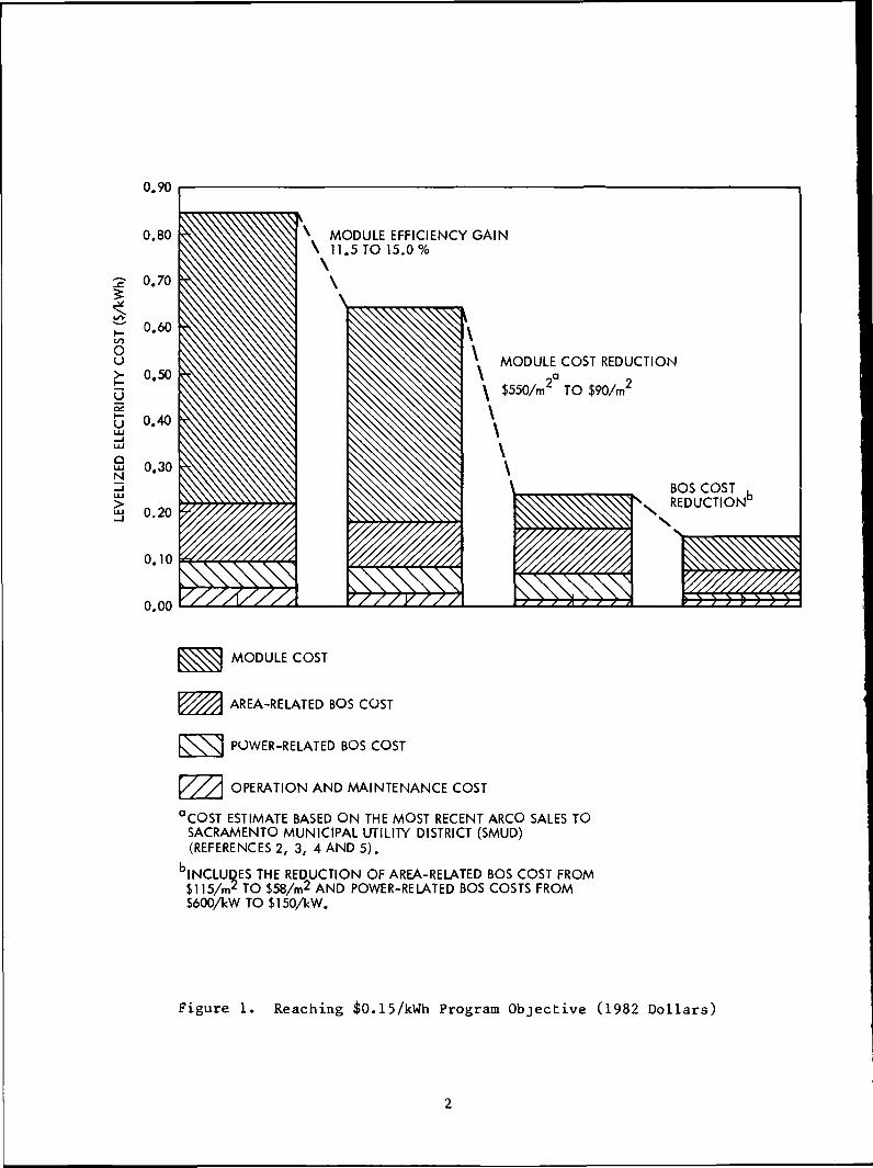
The goals of the DOE Five-Year Research Plan define a path for thedevelopment of a competitive PV technology. Beginning with today's PVsystems, Figure 1 shows how the realization of these goals will produce acompetitive technology. Improved efficiency, module cost reduction, andbalance of system (BOS) cost reduction all play important roles in reachingthe objective. Combined, they are projected to bring about a reduction in thecost of energy produced by PV systems from today's $0.85/kWh to $0.15/kWh,measured as the levelized cost of electricity over the plants' life.
Parameters other than those illustrated in Figure 1 are alsoimportant to PV technology development. Reducing module degradation rates isone good example. Other areas of interest are the trade-offs that existbetween program goals. An examination of these sensitivity questions lead tothe following findings.
-In this study, all levelized costs are in nominal rather than real terms.Nominal levelization closely approximates utility (inflation included)accounting practices; and it is the method which DOE has adopted for nationalprogram planning. The difference between nominal and real levelized costs isdiscussed in Appendix C.
Itoo(J
yQiI—
u
oLLJN
MODULE EFFICIENCY GAIN\ 11.5 TO 15.0%\\
MODULE COST REDUCTION
\ $550/m2 TO $90/m2
MODULE COST
AREA-RELATED BOS COST
POWER-RELATED BOS COST
\///\ OPERATION AND MAINTENANCE COST
°COST ESTIMATE BASED ON THE MOST RECENT ARCO SALES TOSACRAMENTO MUNICIPAL UTILITY DISTRICT (SMUD)(REFERENCES 2, 3, 4 AND 5).
INCLUDES THE REDUCTION OF AREA-RELATED BOS COST FROM$1 15/m2 TO $58/m2 AND POWER-RELATED BOS COSTS FROMS600AW TO $150/kW.
Figure 1. Reaching $0.15/kWh Program Objective (1982 Dollars)
1.2.1 Tracking Configuration
One-axis tracking is an important technical option for reachingprogram goals. For 15% efficient modules, allowable module costs are aminimum of 20% lower for fixed and two-axis tracking configurations. Atcurrent commercial module costs, however, two-axis tracking is optimal.
1.2.2 Solar Insolation and Competing Energy Costs
(1) Solar insolation and EC are specific to geographicallocation. As a result, the selection of specific PV systemcost and efficiency goals limits system applications tocertain geographical markets. Setting higher goals forsystem efficiency and reductions in the cost of systemcomponents ensures a large market for PV. However,increased R&D resources will be required for program success.
(2) Appropriate values for program planning are an energy costgoal of $0.15/kWh and annual insolation values of 2000, 2400,2600 ttWh/m2/yr (fixed array, one-axis tracking, andtwo-axis tracking systems, respectively). With DOE programgoals of $90/m2 for module cost and 15% module efficiency,one-axis tracking systems will be competitive in severalsouthern geographical markets and other locations with highconventional energy costs.
(3) Although the National Photovoltaics Program goals are definedusing specific values for annual solar insolation, highcompeting energy costs in some local markets will makephotovoltaics attractive despite significantly lowerinsolation. Using typical insolation and EC values for eachlocation, Figure 2 shows how high annual insolation in Phoenixraises allowable module cost (maximum that can be paid formodules without system energy costs exceeding goals) wellabove the $90/m^ program goal for a 15% efficient module,despite low EC. In comparison, Miami just falls below theprogram goal at $88/m2 because of lower insolation.Insolation levels are even lower in Long Island than Miami,but as Figure 2 indicates, higher EC raises allowable modulecosts to program goal levels.
1.2.3 Module Cost and Efficiency Trade-offs
(1) High efficiency (e.g., greater than 15%) is neithernecessary, nor is it alone sufficient, for economicallyviable systems (Figure 3). Technologies, such asthin-films, may provide relatively low cost, low efficiencymodules that result in competitive system energy costs. Forexample, the lower curve in Figure 3 indicates that 10%efficient modules would meet program goals for system energycost if they could be produced for $>30/m^. In contrast,many current lower bound estimates for crystalline siliconsolar cell production costs are greater than $90/m2, which

280
240
SS 200cs
toO 160u
8
O
80
40
PHOENIX
(2881 kWh/m2/year)($0.137/kWh)>
PROGRAMGOAL
MIAMI
(2175 kWh/m2/year)($0.161/kWh)
I I I I
,LONG ISLAND
(1900 kWh/m2/year)($0.186/kWh)
10 12 14 16 18
MODULE EFFICIENCY (%)
20 22
Figure 2. Importance of Insolation and Competing Energy Costs (1982 Dollars)
0.80
CURRENT COMMERCIALTECHNOLOGY
11 13 15 17 19 21
MODULE EFFICIENCY (%)
23
Figure 3. Lower Energy Costs Through Lower Module Costs (1982 Dollars)

indicates that some efficiency improvements above programgoals may be required. Accordingly, the program shouldremain flexible in its research program to exploit thetrade-offs between these parameters.
(2) Further reductions in module cost are necessary for developingeconomically viable systems. For current commercial modulecosts of lfc550/m^, Figure 3 shows that increases in moduleefficiency up to 24% and above are not sufficient to reducesystem energy costs to a competitive level, $0.15/kWh. Thesame conclusion can be drawn for modules costing $200/m2,which corresponds to estimated production costs usingstate-of-the-art technology and scaled-up productionfacilities. However, a module costing $120/m^ would becompetitive at an efficiency of approximately 18%.
1.2.4 PV System Parameters and System Energy Cost
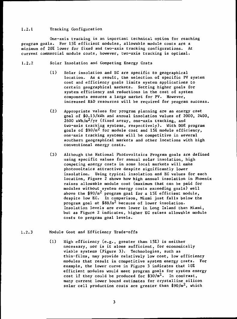
(1) Research advances in several areas of PV technology can leadto significant improvements in the competitiveness of thetechnology. Figure 4 shows how PV system energy costsdecline in response to a 1% reduction in the gap betweencurrent technology and the program goal. For example, a 1%closing of the gap in module cost, $1.10/m , results in a0.284% reduction in PV system costs. This example uses amuch lower value for current module costs, $200/m2 ratherthan the it550/m^ used in Figure 1. Modules can bepurchased commercially for $550/m . However, studies atthe Jet Propulsion Laboratory (JPL) (Reference 6) indicatethat they could be produced for $200/m using the bestavailable technology and large scale production facilities.Tne focus of R&D efforts are on improving the best availabletechnology, so j>200/m2 will be used for the remainder ofthis report.
Closing the gap in module efficiency was found to be almostequally effective in improving the technology's competitive-ness as reductions in module cost. Improvements in area-related BOS cost and power-related BOS cost would only be ahalf or a third as effective as module efficiency gains inmoving the PV technology toward its goals. Nevertheless,their importance cannot be overlooked. If the researchoutlook indicated that dollars spent on BOS research would betwo or three times more effective, these areas would belong onan equal standing with module efficiency research.(Obviously, other considerations must also enter the processof setting research priorities.)
(2) The baseline assumptions for this study are given in Table 1.The information in the table is sufficient to calculate theenergy costs of fixed, one-axis and two-axis PV systems.
MODULE COST
$550 TO 90/m2
MODULE COST
$200 TO 90/m2
MODULE EFFICIENCY
11.5 TO 15.0%
AREA-RELATED BOS COST
$U5TO58/m2
POWER-RELATED BOS COST
$600 TO 150AW
BOS EFFICIENCY
0.836 TO 0.865*
0.635%
0.284%
0.273%
0.079%
0.050%
0.034%
*THE BOS EFFICIENCY VALUES ARE APPROPRIATE WHEN CALCULATING LEVELIZED BUSBAR ENERGY COSTS UNDER THE SPECIFIC ASSUMPTIONS OF THIS STUDY. THEYSHOULD NOT BE INTERPRETED AS THE REAL RANGE OF BOS EFFICIENCIES. THEDERIVATION OF BOS EFFICIENCIES, INCLUDING DEGRADATION. IS GIVEN INAPPENDIX B.
Figure 4. PV System Cost Sensitivity (Response to 1% Closing of GapBetween Current Technology and Program Goals, 1982 Dollars)
A number of revisions of this baseline case have been madesince the original publication of the Five-Year ResearchPlan. The principal implication of these revisions is anincrease in allowable module costs for flat-plate systems froma range of $40-75/m^ as found in the Five-Year Research Planto $90/m2. The crystalline silicon solar cell technologies,which have relatively high manufacturing costs, are now morelikely to fall in the range of allowable module costs.
(3) The indirect cost multiplier, which is a markup on capitalcosts for construction expenses other than labor andmaterials, was set at the same level (1.5) used in theFive-Year Research Plan. A review of the information used toestimate this parameter indicated a wide range of plausiblevalues. Sensitivity of system energy costs and technicalgoals to this parameter make its value an importantconsideration.
(4) The fixed charge rate which provides for the recovery ofcapital investment is reduced from the 0.180 used in theFive-Year Research Plan to 0.153. Improved tax treatment in

Table 1. Technical and Economic Parameters for PVSystem Evaluation (1982 Dollars)
Module Area CostModule Efficiency at STC*Nominal Levelized Energy CostAnnual Insolation:
Fixed ArrayOne-Axis TrackingTwo-Axis Tracking
BOS Efficiencies:
DirtDegradationMismatchOther(includes shadowing, PCU efficiency,AC and DC wiring losses)
Cumulative BOS Efficiency
Area-Related BOS Cost:
Fixed ArrayOne-Axis TrackingTwo-Axis Tracking
Power-Related BOS CostAnnual O&M Cost:
Fixed ArrayTracking
Indirect Cost MultiplierFixed Charge RateCapital Recovery FactorPresent Worth FactorGeneral Inflation RateNominal Discount Rate
$90/rn2
15%$0.15/kWh
2000 kWh/m2/yr2400 kWh/m2/yr2600 kWh/m2/yr
0.970.9630.990.935
0.865
$50/m2
$58/m2
$90/m2
$150/kW AC
$1.10/m2
$1.40/m2
1.50.1530.129188.5%12.5%
*Throughout this report, all module efficiencies are measured with respectto standard test conditions, 1000 kWh/m2/yr irradiance and 25°C celltemperature. A 0.88 temperature adjustment factor, TC, is used in theequation presented in Table 2 to compensate for actual cell temperatures.

terms of the allowed rate of depreciation accounts for thechange. An acceleration of the rate of depreciation allowedon investment, income tax credits, or a reduction in the taxrate will lower the fixed charge rate. Reductions in thefixed charge rate work in favor of PV systems relative toconventional generation technologies because of the greatercapital intensity of PV technology.
(5) Reflecting more recent studies of operation and maintenance(O&M) costs, the estimate has been reduced from $2.28/m2/yrfor flat-plate systems and $2.69/m^/yr for tracking systemsto $1.10/m2/yr and $1.40/m2/yr, respectively. O&M costsare only a small fraction of PV system costs, but widevariations in module replacement rates were found to havesignificant cost implications.

SECTION 2
THE FRAMEWORK
2.1 PURPOSE
The successful development of any new technology such as PVdepends on its economic competitiveness with other technological options. Inorder to provide a framework for the evaluation of PV research and technologydevelopment, the DOE has adopted a revenue requirements methodology forcalculating the cost of energy produced by a PV system (see Reference 1). DOEhas also set a levelized electricity cost goal of $0.15/kWh for energyproduced by central station PV systems. This energy cost is midway betweenthe expected costs of new oil and new coal generation, and is comparable tothe cost of new coal generation at capacity factors typical of intermediateload generation (References 7 and 8). The energy cost goal, therefore,represents widespread commercial viability for PV systems.
The cost of energy produced by a PV plant is a function of manyparameters, including the cost of the plant, O&M costs, meteorologicalconditions, financial factors, and technological performance. This reportinvestigates the sensitivity of the PV system energy cost to changes in theseparameters and the trade-offs between various cost components consistent witha given energy cost goal. The implications of these changes and trade-offsfor the National Photovoltaics Program are also examined.
The purpose of this analysis is to help DOE and industry developcommercially viable central station PV systems. Given the energy cost goal,it is important to analyze the available trade-offs between PV systemcomponents so that component goals can be established in a way that increasesthe likelihood of overall program success. Furthermore, by determining thesensitivity of system energy cost to changes in parameter values, the mostpromising opportunities for PV research and development can be identified.This report shows that substantial progress can be made toward achieving theenergy cost goal by taking advantage of the economic and technicalopportunities and trade-offs that exist for low-cost PV systems. Specificparameter values and technical goals for planning purposes are also reviewedbased on the results of recent research and field studies.
Since module cost and efficiency are the major components of PVenergy cost at this time, and because module development is the most promisingand active research area, the analysis emphasizes trade-offs between modulecost and module efficiency under different economic and technical conditions.In general, this study discusses module cost and performance characteristicsin terms of "allowable" costs and efficiencies, which are the costs andefficiencies that are consistent with a given energy cost goal.
2.2 APPROACH
Life-cycle energy cost is an appropriate measure for evaluating PVresearch progress and economic viability. With this approach, the futurevalue of the new technology can be used directly in the process of setting

research and development priorities. Furthermore, "comparing conceptualdesigns and cost estimates of a new technology with those of a currentlyavailable technology gives insight into the cost incentives and technicalissues associated with the new technology" (Reference 9).
Annualized life-cycle costs of a central station PV generatingsystem can be calculated using the expression in Table 2. The left side ofthe expression summarizes the annual capital and operating needs of thesystem. The right side of the equation summarizes the value of the output,where EC measures energy cost and the remainder of the expression representsannual output. The cost calculated with this expression is the cost ofelectricity that the system will be able to compete with. If the cost is wellabove the expected cost for conventional generating plants, then significantuse of the technology by electric utilities cannot be expected. Conversely,if the cost is below what is projected for conventional generating plants,then electric utilities can be expected to include PV in their investmentplans^. (Of course, factors other than cost will also influence theirdecisions; see Reference 8.)
With the aid of this expression, several areas of uncertaintyaffecting the future of the technology can be explored. One area is thetrade-offs between the parameters which determine the cost of the PV system.For example, how much of a reduction in area-related BOS cost ($MSQBS) isneeded to offset an increase in module cost ($MSQMD)? This is easilycalculated using the equation in Table 2 by holding the remaining parametersconstant, and finding the combination of $MSQMD and $MSQBS that maintain theequality. Another important area of uncertainty is the cost of competingenergy. Holding everything else unchanged, energy cost can be increased andthe allowable increase in module cost calculated. The expression forcalculating life-cycle energy cost includes three financial parameters: thefixed charge rate (FCR), the present worth factor (G) and the capital recoveryfactor (CRF). These parameters can be varied to determine the consequencesfor another parameter such as module cost. However, considerable care has tobe taken when changing the financial parameters. The energy cost forcompeting technologies may also be affected by the same financial parameters.
2.3 DATABASE
In the process of investigating the sensitivity of individualparameters, an extensive database was constructed. The database includesvalues used for the technical parameters found in the expression forannualized life-cycle energy cost, and values appropriate for characterizingsolar energy availability, EC, and financial conditions. The values settledupon for this study were given previously in Table 1.
^Papay, L.T., Southern California Edison Co., "The Electric Utilities andPhotovoltaics: Financing and Integration," Rosemead, California (preparedfor 2nd International Conference on Photovoltaic Business Development,Geneva, Switzerland, May 18, 1983).
10

Table 2. Revenue Requirements Methodology
($MSQMD + $MSQDS + KWBS\ INDC'FCR + $MSQOM'G'CRF = EC'INSOL
A / A-PKI2
$MSQMD = module costs in $/mo
$MSQBS = balance of system area-related costs in $/m
$KWBS = balance of system power-related costs in $/kW AC
INDC = indirect cost multiplier
FCR = annual fixed charge rate (includes the cost of debt and equitycapital, taxes, allowable depreciation and tax credits)
2$MSQOM = annual operation and maintenance costs in $/m -yr
G = present worth factor for recurring O&M costs (function of costescalation rate, discount rate and system lifetime)
CRF = capital recovery factor (a function of the discount rate and systemlifetime)
£C = levelized cost of electricity in $/kWh2
INSOL = annual insolation in kWh/m
A = 1/(TC-BOSE-EFF-PKI)*
*A is the plant aperture area required to generate IkW of AC power at thebusbar under typical operating conditions. A is a function of the effectof temperature on cell efficiency (TC), balance of system efficiency (BOSE),module efficiency (EFF), and average peak insolation (PKI) infor the location.
The starting point for developing the set of parameters found inTable 1 was an Electric Power Research Institute (EPRl) investigation of PVsystem requirements (see Reference 7). The results of this EPRI study wereused in the preparation of the Five-Year Research Plan. Since that time,several efforts have been made to revise and update these parameters and theFive-Year Plan energy cost equation, based on the latest research findings(Reference 10) » . Finally, the interim results of the sensitivity analysiswere used to arrive at what are believed to be the most realistic goals for PV
^Borden, C., Jet Propulsion LaDoratory, "Recommended Parameter Values forthe Five-Year Research Plan," Photovoltaics Program MemoPAIC:CSB:720-84-1697, Pasadena, California, February 13, 1984.
^Crosetti, M., Jet Propulsion Laboratory, "The Indirect Costs of CentralStation Photovoltaic Power Plants," JPL Memo 311.3-1429/2564E, July 19, 1985.
11

program research. The sensitivity analysis made it possible to explore thetrade-offs between different system parameters made practical by recenttechnology improvements.
Sensitivity studies for individual parameters found in theremaining sections of this report include discussions of how the value foreach parameter was attained. This information is often relevant to the rangeof sensitivities that should be explored. In addition, the information isoften useful in deciding upon which trade-offs need to be considered.
12

SECTION 3
KEY TRADE-OFFS AND COMPETING ENERGY COSTS
3.1 DIRECTION
Significant gains in PV module efficiency and cost are required tomake PV competitive with conventional generating systems in central stationapplications. Goals set by the National Photovoltaics Program in both areasrepresent major improvements over current technology. This is true both interms of what is commercially produced today and what could be produced usingthe best available technology. Fortunately, the goals are relaxed somewhat bythe fact that exceptional gains in one area such as module efficiency can betraded off against less success in the area of module cost. Furthermore,additional trade-offs exist with the goals set for the remaining elements ofthe PV system, BOS cost and efficiency. These critical sensitivities are thefirst topic covered in this section.
The competitiveness of a PV system in a central stationapplication depends to a large extent on geographic location (e.g.,insolation and EC costs), and the outlook for conventional energy costescalation. Higher insolation values, like those found in the desertSouthwest, and higher conventional energy costs, like those found in theNortheast, work in favor of PV systems. The selection of a trackingconfiguration, fixed, one-axis, or two-axis tracking, also influence theeconomics of PV systems in central station applications. The combination ofa good geographic location, the prospect of rapidly escalating conventionalenergy costs, and the selection of the best tracking option can greatlyimprove PV system economics. The remainder of this section looks at howeach of these factors affect the goals that have been set for the NationalPhotovoltaics Program.
Because of recent reductions in estimates of area-related BOScosts for one-axis tracking equipment, these systems seem to be the mosteconomically promising over a large range of module efficiencies.Consequently, most of the analysis is concerned with one-axis systems.However, fixed array and two-axis systems are analyzed in the section onannual insolation because the values of this parameter depend on the trackingconfiguration of the system. In particular, high cost modules, such as thosecommercially available today, often produce the cheapest energy when used insystems with two-axis tracking.
3.2 PV SYSTEM COST SENSITIVITY
The cost of PV modules and their efficiency are the two mostcritical elements of system energy cost. Not only is a large portion of thelife-cycle energy cost related to these factors, but they also exhibit thegreatest potential for improvements through research. Current commercial
13

module costs are $550/m2 for 11.5% efficient modules.^ The DOE target is$90/m2 for a 15% efficient module which may be acnievable with several PVtechnologies in the 1990s. Progress in lowering module costs and raisingefficiency is essential if central station PV systems are to becomecommercially viable on a large scale. Competitive energy costs are the onlyother parameter that influences the prospects for PV to such an extent.
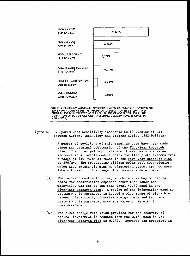
The sensitivity of system energy cost to changes in several areasof PV system technology are illustrated in Figure 5. The top cnart shows howa percentage change in specific system parameters with all other parametersheld at recommended goal levels (see Table 2) impacts system energy cost. Forexample, if module costs fall 40% short of the recommended goal of $90/m2,tne result would be approximately a 20% increase in system energy costs. Incomparison, if module efficiency falls 40% short of the goal value of 15%,system energy costs rise 60%. System energy costs are just as sensitive toBOS efficiency, but this value would not be expected to experience this largeof percentage variation from recommended goal values. Figure 5 also showsthat PV system energy costs will be least affected on a percentage basis byarea-related and power-related BOS cost variances.
The relationships between system energy cost and changes in systemparameters depend on the frame of reference chosen. In the top chart, changesin the absolute level of each parameter were considered, beginning at recom-mended goal levels. The lower chart shows how these sensitivities change ifthe frame of reference is moved to system parameters achievable with currenttechnology, and parameter changes tnat would lessen the gap between currenttechnology and program goals. For example, modules could be produced for aslittle as $200/m2 today (see Reference 6) compared to the current programobjective of $90/m2. If that gap were closed by 40%, $44/m2 (40% ofdifference between $200/m2 and ij>90/m2), system energy cost would bereduced by approximately 25%. The same percentage improvement in moduleefficiency is not nearly as effective in reducing system energy cost,reflecting the smaller disparity between currently achievable technology(11.5%) and the goal for the program (15%). Obviously, these sensitivitieswill also depend on the technology being examined.
PV system energy cost sensitivities, including those used in theconstruction of Figure 5, are presented in Table 3. The sensitivity of systemenergy cost to various cost categories are given first. For example, a 1%reduction in module cost from current state-of-the-art levels ($2 for modulescosting it200/m2) will lower system energy cost by 0.502%. in comparison, a1% reduction in the gap between current technology and the program goal lowerssystem energy cost by 0.305%. The relationship of each of these costcategories to system energy cost is linear. Therefore, a 10% increase inmodule cost from the current level increases the system energy cost by 5.02%.
efficiency number is based on ARCO Solar Incorporated (ARCO) M-53modules. The cost figure is based on ARCO module sales to SMUD (seeReferences 2, 3, 4 and 5).
14
-40 0 20 60 100 200PERCENT CHANGE IN SYSTEM PARAMETER
AREA-RELATEDBOS COST
POWER-RE LA TEDBOS COST
300
oU
OO£UJZUJ
5
V)
zUJozu
100
60
20
0
-20
-60
-100
-140
POWER-RELATEDBOS COST
\
I I-300
7AREA-RELATEDBOS COST
MODULEEFFICIENCY
I I I I I I I I I
BEST CURRENTTECHNOLOGY
-200 -80 -40 0 20
PERCENT CHANGE IN SYSTEM PARAMETER BASED ONGAP BETWEEN CURRENT AND GOAL LEVEL
60 100
Figure 5. PV System Cost Sensitivity to Changes in System Parameters
15

Table 3. PV System Cost Sensitivity to Changes in System Parameters
Resulting Percentage Change in PV System Cost
1% Change in:
Module CostArea-Related BOS CostPower-Related BOS CostIndirect Cost MultiplierO&M Cost
Percent Change inEfficiency Parameter:
+60%+40+20+10-10-20-40-60
Based onCurrentValues*
0.5020.3230.0960.9210.079
Based onCurrentValues*
Moduleor BOS
Efficiency
-32.8-25.0-14.6- 8.09.721.958.4131.3
GoalValues*
0.5110.2940.1250.9300.070
GoalValues*
Moduleor BOS
Efficiency
-33.9-25.8-15.1- 8.210.022.660.3135.7
Gap Between
0.3050.1460.0940.2690.044
Gap Between
ModuleEfficiency
Only
-13.5- 9.5- 5.0- 2.62.75.712.119.6
Values
Values
BOSEfficiencyOnly
-1.8-1.2-0.6-0.30.30.61.21.9
*Tne current and goal values for each parameter are: module cost($200-$90/m2), area-related BOS cost ($115-$58/m2), power-related BOScost ($600-$150/kW), indirect cost multiplier (2.11-1.50), OfcM cost ($3.8 to$1.4/m2), module efficiency (11.5 to 15.0%), and BOS efficiency(83.6 to 86.5%).
The relationship between changes in module efficiency or BOSefficiency and system energy cost is nonlinear. Accordingly, severalindividual sensitivities are given in Table 3 to show how system energy costsrespond over a fairly wide range of changes. When considering the gap thatneeds to be closed between current values and program goals, separate valuesare needed for module and BOS efficiency. The values in this case aredifferent because the gap to be closed in BOS efficiency is relatively smallerthan for module efficiency. Closing the gap in module efficiency will lowersystem energy cost more than closing the gap in BOS efficiency.
16
IFor a given percentage improvement from current values, system
energy costs are most sensitive to module and BOS efficiency changes. Systemefficiency affects not only the total module costs of a PV system, but totalarea-related BOS costs and annual O&M costs as well. (Lower efficiencyrequires more module area to maintain a given plant output rating; therefore,the amount spent on modules, area-related BOS items, and O&M will increase.)In comparison, changes in module cost do not affect the total amounts spent onother plant items.
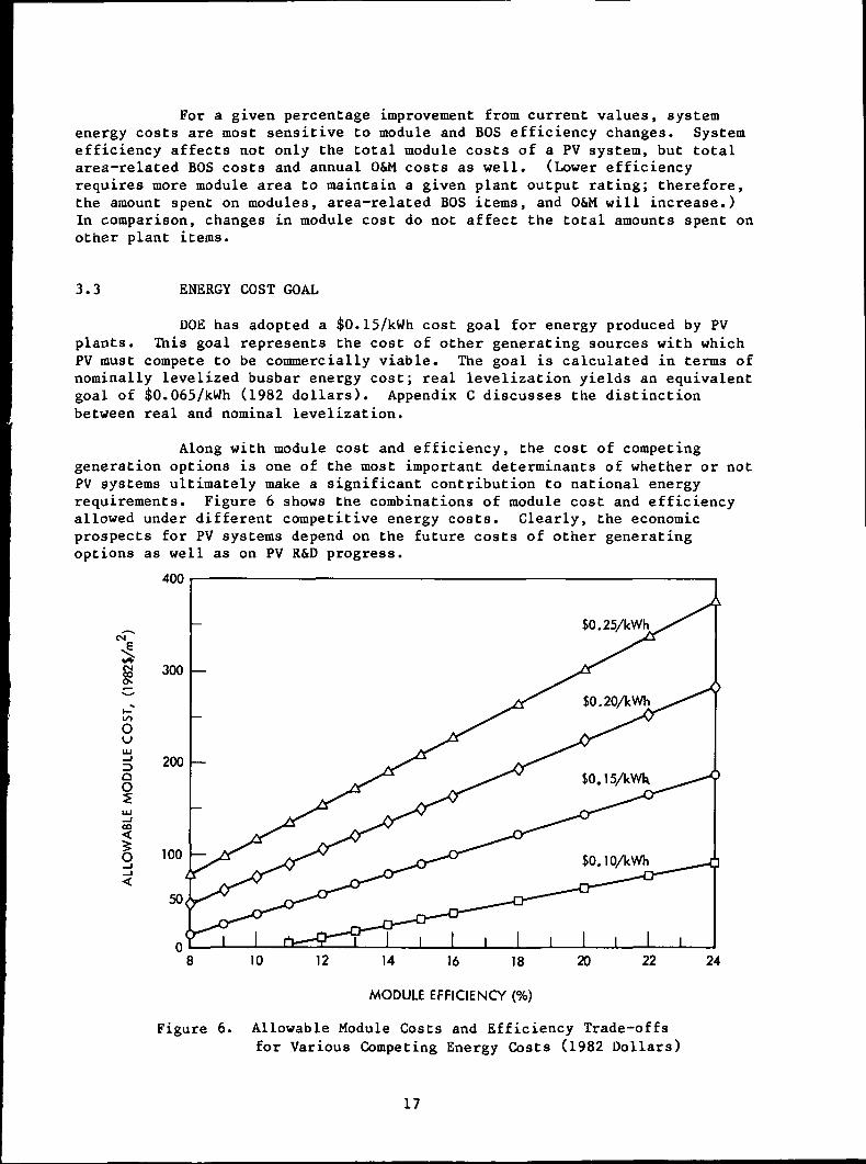
3.3 ENERGY COST GOAL
DOE has adopted a $0.15/kWh cost goal for energy produced by PVplants. This goal represents the cost of other generating sources with whichPV must compete to be commercially viable. The goal is calculated in terms ofnominally levelized busbar energy cost; real levelization yields an equivalentgoal of $0.065/kWh (1982 dollars). Appendix C discusses the distinctionbetween real and nominal levelization.
Along with module cost and efficiency, the cost of competinggeneration options is one of the most important determinants of whether or notPV systems ultimately make a significant contribution to national energyrequirements. Figure 6 shows the combinations of module cost and efficiencyallowed under different competitive energy costs. Clearly, the economicprospects for PV systems depend on the future costs of other generatingoptions as well as on PV R&D progress.
400
5ssLO
Ou
O
i
10 12 14 16 18
MODULE EFFICIENCY (%)
20 22 24
Figure 6. Allowable Module Costs and Efficiency Trade-offsfor Various Competing Energy Costs (1982 Dollars)
17

The $0.15/kWh goal corresponds to a large penetration for PV intothe peaking and intermediate load energy markets in areas with sufficientinsolation. A higher goal would represent a smaller market as there would befewer cases in which PV would be competitive. An appropriate goal is one thatrepresents the desired market for PV. As EPRI points out, "Technology goalsmust be set in conjunction with an estimate of the desired market" (seeReference 8). In this respect, DOE's energy cost goal, insolation levels forplanning, and energy cost equation are useful for determining the variouseffects of market size on technical goals.
If less ambitious market penetration is desired for the researchprogram, then a higher value should be adopted. Scenarios of higher pricedcoal and residual fuel oil generation suggest an energy cost goal of$0.20/kWh. This change would have a tremendous impact on module cost andefficiency goals as indicated in Figure 6.
Before PV systems will be considered in electric utility expansionplans, they will have to be competitive on a cost basis with the conventionalgenerating options open to the utility. Earlier studies have shown thatoutput of PV systems are best suited for meeting the intermediate loadrequirements of electric utilities. In today's market, the lowest costconventional option for capacity expansion is coal. (Nuclear power was notconsidered because of legal and environmental problems confronting thetechnology.) A coal-fired plant meeting the intermediate load requirements ofa utility would have a capacity factor of about 0.30. Therefore, competingenergy costs have been estimated on the basis of a new coal-fired plantoperating with a capacity factor of 0.30.
The revenue requirements of a future coal plant depend on a set ofrelatively uncertain parameters that vary with location. The cost ofconstructing a coal-fired plant and the cost of the coal burned depend on theregion of the country where the plant is located. Also, life-cycle energycosts are quite sensitive to cost escalation rates assumed for fuel and plantinvestment. These considerations can be incorporated into a life-cyclecosting methodology similar to the one that was used for calculating PV systemenergy costs.
Different possible life-cycle energy costs for coal-fired plantsmeeting intermediate load requirements are given in Table 4. The tableillustrates how these cost estimates vary by region of the country anddifferent assumed escalation rates for capital and fuel costs. The costestimates in this table are based on capital cost and O&M cost estimates takenfrom the EPRI Technical Assessment Guide (see Reference 9). Fuel costs werederived from industry journals (Reference 11).
The energy cost values in Table 4 indicate that PV systems will becompetitive in the Northeast if program goals are met and sufficientinsolation is available. For the Pacific and Rocky Mountain regions whereinsolation is not exceptional, PV systems would be competitive only whereescalation rates for capital and fuel costs are projected to be high enough.Figure 7 gives some perspective on how the energy cost goal for the NationalPhotovoltaics Program compares to the outlook for coal-fired generation costs,serving as intermediate load capacity. Although the figure alone cannot be
18

Table 4. Levelized Costs of Coal-Generated Power for MeetingIntermediate Loads (Dollars/kWh)
RegionCapital CostEscalation, %
Fuel Cost Escalation,
Northeast*
Pacific*
Rockies*
0135
0135
0135
0.1530.1590.1730.188
0.1190.1250.1390.156
0.1110.1170.1320.148
0.1670.1720.1860.201
0.1250.1320.1460.162
0.1160.1220.1370.153
0.1830.1890.2020.218
0.1340.1400.1540.170
0.1220.1290.1430.159
0.2030.2090.2220.238
0.1440.1500.1640.180
0.1300.1360.1510.167
*The following conditions were assumed for each region, based on Reference 8.
Northeast Pacific Rockies
Fixed O&M $/kW/yrVariable/Consumables O&M $/kWhCapital Cost $/kWhFuel Cost $/Ton (Reference 10)Heat Rate kWh/TonWorking Capital Cost Markup
16.10.0037
109052
21621.2
14.50.0024
115026
21621.2
14.50.0024
115020
21621.2
used to determine specific energy markets for PV, it gives some indication ofthe breadth of markets that would be available and how their number would beaffected by capital and fuel escalation rates.
A smaller initial market for PV may be considered by adopting a costgoal based on competition with higher priced coal generation or with residualfuel oil generation. A recent study found that over 3,000 MW of new oil andgas-fired generating capacity is planned for the next ten years (Reference 12).Table 5 presents residual oil combustion turbine energy cost scenarios fordifferent fuel cost trends with conventional and advanced plant designs. Thecombustion turbine is typical of peaking plants. Table 5 also presents energycost scenarios for both conventional and advanced residual oil combined cycleplants, which are intermediate load generators.
19

0.30
IO 0.25CtL
O§£ 0.20
gO.15
Ou
0.10
ROCKIESI
u.sAVERAGE
HIGHESCALATION5% CAPITAL2% FUEL
MEDIUMESCALATION
LOWESCALATION1% CAPITAL0% FUEL
NORTHEAST
20 40
COST OF COAL ($/Ton)
60 80
Figure 7. The Outlook for Intermediate Load Energy Costs and Achievingthe PV Program Energy Cost Goal (1982 Dollars)
In summary, the cost of competing energy in a particular utilityapplication can vary significantly from the national program goal of$0.15/ktfh. For example, regional differences exist in the cost of electricityfrom new coal plants. Utilities are likely to vary in their opinion as towhat the cost of coal-generated electricity will be, based on their outlookfor fuel and capital cost increases. Also, some utilities may be consideringcombined cycle oil-fired plants for intermediate load capacity. Inapplications where PV will be serving peak load requirements, the cost of newcombustion turbine plants enter the picture. The cost of electricity fromthese generating technologies is also sensitive to the outlook for capital andfuel cost escalation.
3.4 INSOLATION
Insolation values at a particular geographic location combine with
the outlook for competing energy costs to determine the economic viability ofa PV system. Insolation available on an annual basis can vary by as much as afactor of two between different locations in the United States, although thedifferences between most locations is considerably smaller. PV systems will
20

Table 5. Levelized Costs of Energy Generated by Combustion Turbine andCombined Cycle Oil-Fired Generators (Dollars/kWh)
Capital CostEscalation (%)
Conventional Oil Combustion Turbine*
0135
Advanced Oil Combustion Turbine*
0135
Conventional Combined Cycle Oil*
0135
Advanced Combined Cycle Oil*
0135
*The following conditions were assumedReference 8:
Fixed O&M 1980 $/kW/yrVariable/Consum. O&M 1980 $/kWhCapital Cost 1980 $/kWFuel Cost 1980 fc/mmBTUCapacity FactorHeat Rate BTU/kWhWorking Capital Cost Markup
Fuel Cost Escalation (%)
-1
0.1860.1870.1910.194
0.1710.1720.1760.180
0.1380.1410.1470.154
0.1280.1310.1370.145
for each
Conven-tionalCT
0.40.0037
2355.15
0.261140001.2
0
0.2260.2270.2300.234
0.2060.2080.2120.216
0.1630.1660.1720.179
0.1500.1530.1590.167
technology
AdvancedCT
0.40.0037
2555.150.267126001.2
1
0.2730.2740.2770.281
0.2490.2500.2540.258
0.1920.1950.2010.208
0.1750.1780.1850.192
based on
Conven-tionalCC
6.60.0016
4955.150.386851.2
2
0.3320.3330.3360.340
0.3020.3030.3070.311
0.2290.2310.2370.245
0.2070.2100.2170.224
AdvancedCC
6.60.0016
5305.150.376201.2
21
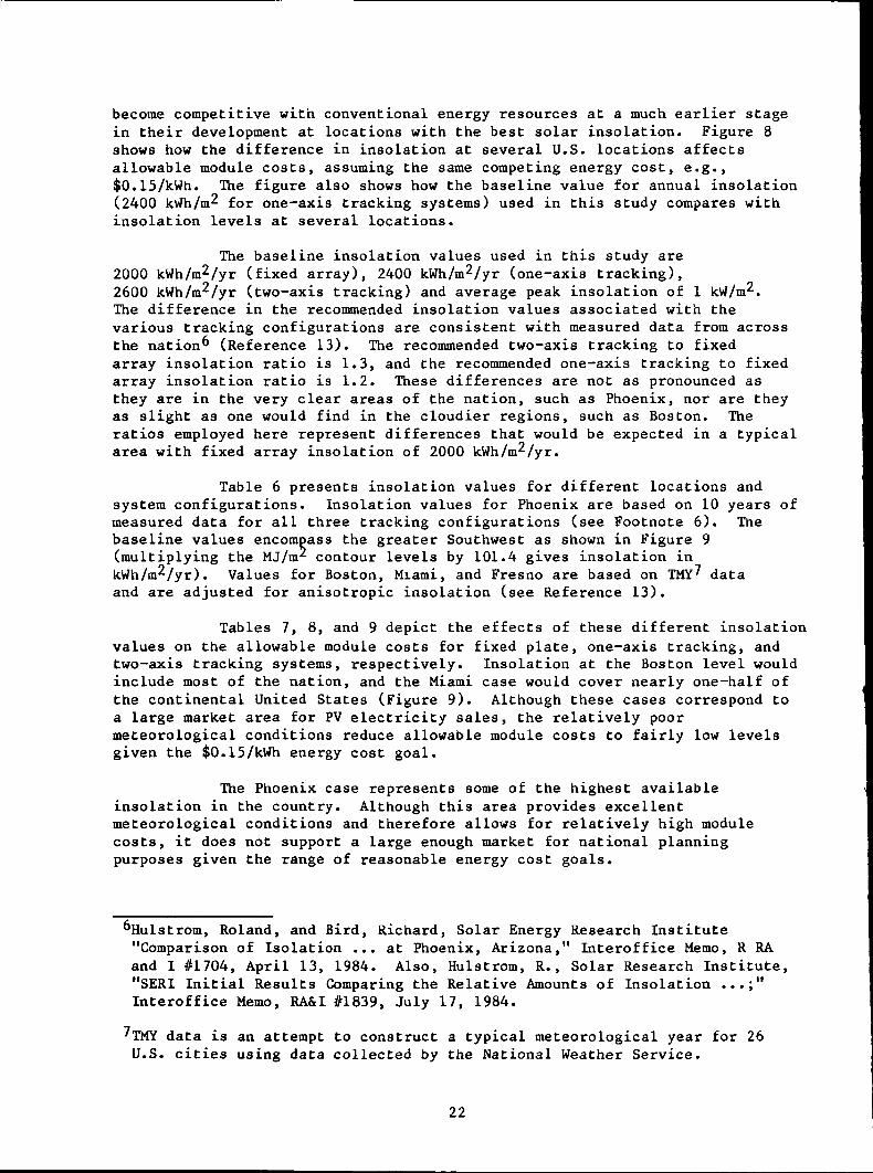
become competitive with conventional energy resources at a much earlier stagein their development at locations with the best solar insolation. Figure 8shows how the difference in insolation at several U.S. locations affectsallowable module costs, assuming the same competing energy cost, e.g.,$0.15/kWh. The figure also shows how the baseline value for annual insolation(2400 ktfh/m2 for one-axis tracking systems) used in this study compares withinsolation levels at several locations.
The baseline insolation values used in this study are2000 kWh/m2/yr (fixed array), 2400 kWh/m2/yr (one-axis tracking),2600 kWh/m2/yr (two-axis tracking) and average peak insolation of 1 kW/m2.The difference in the recommended insolation values associated with thevarious tracking configurations are consistent with measured data from acrossthe nation^ (Reference 13). The recommended two-axis tracking to fixedarray insolation ratio is 1.3, and the recommended one-axis tracking to fixedarray insolation ratio is 1.2. These differences are not as pronounced asthey are in the very clear areas of the nation, such as Phoenix, nor are theyas slight as one would find in the cloudier regions, such as Boston. Theratios employed here represent differences that would be expected in a typicalarea with fixed array insolation of 2000 kWh/m2/yr.
Table 6 presents insolation values for different locations andsystem configurations. Insolation values for Phoenix are based on 10 years ofmeasured data for all three tracking configurations (see Footnote 6). Thebaseline values encompass the greater Southwest as shown in Figure 9(multiplying the MJ/m2 contour levels by 101.4 gives insolation inkWh/m2/yr). Values for Boston, Miami, and Fresno are based on TMY^ dataand are adjusted for anisotropic insolation (see Reference 13).
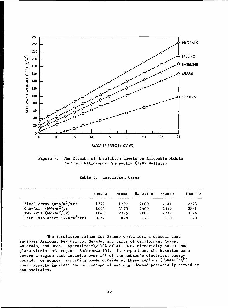
Tables 7, 8, and 9 depict the effects of these different insolationvalues on the allowable module costs for fixed plate, one-axis tracking, andtwo-axis tracking systems, respectively. Insolation at the Boston level wouldinclude most of the nation, and the Miami case would cover nearly one-half ofthe continental United States (Figure 9). Although these cases correspond toa large market area for PV electricity sales, the relatively poormeteorological conditions reduce allowable module costs to fairly low levelsgiven the $0.15/kWh energy cost goal.
The Phoenix case represents some of the highest availableinsolation in the country. Although this area provides excellentmeteorological conditions and therefore allows for relatively high modulecosts, it does not support a large enough market for national planningpurposes given the range of reasonable energy cost goals.
"Hulstrom, Roland, and Bird, Richard, Solar Energy Research Institute"Comparison of Isolation ... at Phoenix, Arizona," Interoffice Memo, R RAand I #1704, April 13, 1984. Also, Hulstrom, R., Solar Research Institute,"SERI Initial Results Comparing the Relative Amounts of Insolation ...;"Interoffice Memo, RA&I #1839, July 17, 1984.
'TMY data is an attempt to construct a typical meteorological year for 26U.S. cities using data collected by the National Weather Service.
22
PHOENIX
10 12 14 16 18 20
MODULE EFFICIENCY (%)
22 24
Figure 8. The Effects of Insolation Levels on Allowable ModuleCost and Efficiency Trade-offs (1982 Dollars)
Table 6. Insolation Cases
Boston Miami Baseline Fresno Phoenix
Fixed Array (kWh/m2/yr)One-Axis (kWh/m2/yr)Two-Axis (kWh/m2/yr)Peak Insolation (kWh/m2/yr)
1377166518430.67
1797217523150.8
2000240026001.0
2141258527791.0
2223288131981.0
The insolation values for Fresno would form a contour thatencloses Arizona, New Mexico, Nevada, and parts of California, Texas,Colorado, and Utah. Approximately 10% of all U.S. electricity sales takeplace within this region (Reference 15). In comparison, the baseline casecovers a region that includes over 14% of the nation's electrical energydemand. Of course, exporting power outside of these regions ("wheeling")could greatly increase the percentage of national demand potentially served byphotovoltaics.
23

t>0c•Hy<B[*•
C/3 0)y
« e0)
C fl)O 06
•8
oM5
0) Uj3 n)o Jr-l
O II
• t-l -Hn Ho0) 0)oo y
> 3< cn
bO
24

Table 7. Allowable Fixed Array Module Cost (1982 Dollars/m2)
Annual Insolation (kWh/m2/yr)Peak Insolation (kW/m2)
Module Efficiency
0.080.090.100.110.120.130.140.150.160.180.200.220.24
Boston
13770.67
Miami
17970.8
Baseline
20001
Allowable Module
-12- 606121824303648617385
311192735435159678399115132
9182736455362718097115133150
Fresno
21411
Cost
152434435363728291110129148167
Phoenix
22231
182838485868788898117137157177
Table 8. Allowable One-Axis Tracking Module Cost (1982 Dollars/m2)
Annual Insolation (kWh/m2/yr)Peak Insolation (kW/m2)
Module Efficiency
0.080.090.100.110.120.130.140.150.160.180.200.220.24
Boston
16650.67
Miami
21750.8
Baseline
24001
Allowable Module
-12- 43
111826334148637893108
71727374757677686106126146166
1425364757687990101122144165187
Fresno
25851
Cost
22334557688092104115139162186209
Phoenix
28811
334760738699113126139165192218244
25
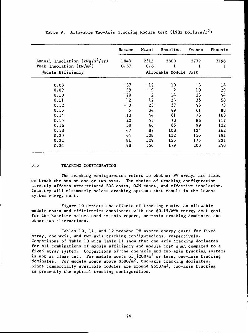
Table 9. Allowable Two-Axis Tracking Module Cost (1982 Dollars/m2)
Boston Miami Baseline Fresno Phoenix
Annual Insolation (kWh/m2/yr)Peak Insolation (kW/m2)
Module Efficiency
0.080.090.100.110.120.130.140.150.160.180.200.220.24
18430.67
-37-29-20-12- 35
13223047648198
2315 26000.8 1
Allowable Module
-19- 9212233444556687108129150
-10214263749617385108132155179
27791
Cost
-31023354861738699124150175200
31981
142944587388103117132162191221250
3.5 TRACKING CONFIGURATION
The tracking configuration refers to whether PV arrays are fixedor track the sun on one or two axes. The choice of tracking configurationdirectly affects area-related BOS costs, O&M costs, and effective insolation.Industry will ultimately select tracking options that result in the lowestsystem energy cost.
Figure 10 depicts the effects of tracking choice on allowablemodule costs and efficiencies consistent with the $0.15/kWh energy cost goal.For the baseline values used in this report, one-axis tracking dominates theother two alternatives.
Tables 10, 11, and 12 present PV system energy costs for fixedarray, one-axis, and two-axis tracking configurations, respectively.Comparisons of Table 10 with Table 11 show that one-axis tracking dominatesfor all combinations of module efficiency and module cost when compared to afixed array system. Comparisons of the one-axis and two-axis tracking systemsis not as clear cut. For module costs of $200/m or less, one-axis trackingdominates. For module costs above $300/m2, two-axis tracking dominates.Since commercially available modules are around $550/m2, two-axis trackingis presently the optimal tracking configuration.
26

200
10 12 14 16 18
MODULE EFFICIENCY (%)
20 22 24
Figure 10. Allowable Module Cost and Efficiency Trade-offs forAlternative Tracking Configurations (1982 Dollars)
Table 10. Levelized Energy Costs for a Fixed ArrayConfiguration (Dollars/kWh)
Module Efficiency Module Cost
0.030.060.080.090.100.110.120.130.140.150.160.180.200.220.24
30 60 90 120 200 300 550
Energy Cost
0.480.250.190.170.150.140.13
0.630.320.250.220.200.180.170.160.150.14
0.780.400.300.270.250.220.210.190.180.170.160.140.130.120.11
0.930.470.360.320.290.270.240.230.210.200.190.170.150.140.13
1.330.670.510.450.410.380.350.320.300.280.260.240.210.200.18
0.620.560.510.470.440.410.380.360.320.290.260.24
0.850.780.730.680.630.590.530.480.440.40
27
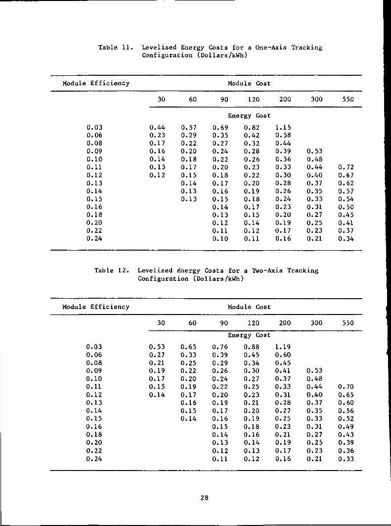
Table 11. Levelized Energy Costs for a One-Axis TrackingConfiguration (Dollars/kWh)
Module Efficiency
30 60
Module Cost
90 120 200 300 550
Energy Cost
0.0.0.0.0.0.0.0.0.0.0.0.0.0.0.
030608091011121314151618202224
0.0.0.0.0.0.0.
44231716141312
0.0.0.0.0.0.0.0.0.0.
57292220181715141313
0.690.350.270.240.220.200.180.170.160.150.140.130.120.110.10
0.820.420.320.280.260.230.220.200.190.180.170.150.140.120.11
100000000000000
.15
.58
.44
.39
.36
.33
.30
.28
.26
.24
.23
.20
.19
.17
.16
0.530.480.440.400.370.350.330.310.270.250.230.21
0.720.670.620.570.540.500.450.410.370.34
Table 12. Levelized Energy Costs for a Two-Axis TrackingConfiguration (Dollars/kWh)
Module Efficiency
0.030.060.080.090.100.110.120.130.140.150.160.180.200.220.24
30 60
0.53 0.650.27 0.330.21 0.250.19 0.220.17 0.200.15 0.190.14 0.17
0.160.150.14
Module Cost
90 120 200 300 550
Energy Cost
0.76 0.88 1.190.39 0.45 0.600.290.260.240.220.200.190.170.160.150.140.130.120.11
0.340.300.270.250.230.210.200.190.180.160.140.130.12
0.450.410.370.330.310.280.270.250.230.210.190.170.16
0.530.480.440.400.370.350.330.310.270.250.230.21
0.700.650.600.560.520.490.430.390.360.33
28
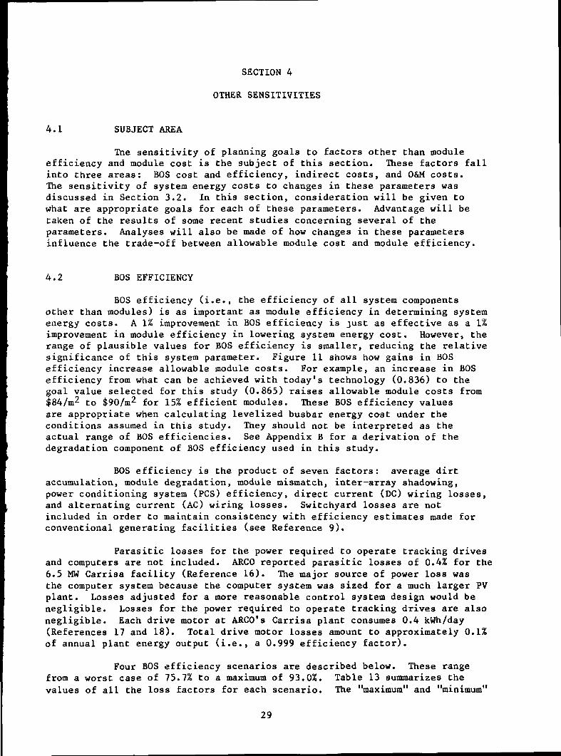
SECTION 4
OTHER SENSITIVITIES
4.1 SUBJECT AREA
Tne sensitivity of planning goals to factors other than moduleefficiency and module cost is the subject of this section. These factors fallinto three areas: BOS cost and efficiency, indirect costs, and O&M costs.The sensitivity of system energy costs to changes in these parameters wasdiscussed in Section 3.2. In this section, consideration will be given towhat are appropriate goals for each of these parameters. Advantage will betaken of the results of some recent studies concerning several of theparameters. Analyses will also be made of how changes in these parametersinfluence the trade-off between allowable module cost and module efficiency.
4.2 BOS EFFICIENCY
BOS efficiency (i.e., the efficiency of all system componentsother than modules) is as important as module efficiency in determining systemenergy costs. A 1% improvement in BOS efficiency is just as effective as a 1%improvement in module efficiency in lowering system energy cost. However, therange of plausible values for BOS efficiency is smaller, reducing the relativesignificance of this system parameter. Figure 11 shows how gains in BOSefficiency increase allowable module costs. For example, an increase in BOSefficiency from what can be achieved with today's technology (0.836) to thegoal value selected for this study (0.865) raises allowable module costs from$84/m2 to $90/m2 for 15% efficient modules. These BOS efficiency valuesare appropriate when calculating levelized busbar energy co-st under theconditions assumed in this study. They should not be interpreted as theactual range of BOS efficiencies. See Appendix B for a derivation of thedegradation component of BOS efficiency used in this study.
BOS efficiency is the product of seven factors: average dirtaccumulation, module degradation, module mismatch, inter—array shadowing,power conditioning system (PCS) efficiency, direct current (DC) wiring losses,and alternating current (AC) wiring losses. Switchyard losses are notincluded in order to maintain consistency with efficiency estimates made forconventional generating facilities (see Reference 9).
Parasitic losses for the power required to operate tracking drivesand computers are not included. ARCO reported parasitic losses of 0.4% for the6.5 MW Carrisa facility (Reference 16). The major source of power loss wasthe computer system because the computer system was sized for a much larger PVplant. Losses adjusted for a more reasonable control system design would benegligible. Losses for the power required to operate tracking drives are alsonegligible. Each drive motor at ARCO's Carrisa plant consumes 0.4 kWh/day(References 17 and 18). Total drive motor losses amount to approximately 0.1%of annual plant energy output (i.e., a 0.999 efficiency factor).
Four BOS efficiency scenarios are described below. These rangefrom a worst case of 75.7% to a maximum of 93.0%. Table 13 summarizes thevalues of all the loss factors for each scenario. The "maximum" and "minimum"
29

10 12 14 16 18 20
MODULE EFFICIENCY (%)
22 24
Figure 11. Allowable Module Cost and Efficiency Trade-offfor Different BOS Efficiencies (1982 Dollars)
Taole 13. BOS Efficiency Cases
Mechanism Maximum Baseline Low
Total Product 0.930 0.865 0.810
Minimum
DirtDegradationMismatchPCS efficiencyShadowDC efficiencyAC efficiency
0.990.9700.9950.980.9980.995
*
0.970.9630.990.950.990.994
*
0.950.950.970.950.9850.9940.995
0.940.9440.970.930.970.980.995
0.757
In these scenarios, AC efficiency is included in PCS efficiency.
30

values correspond to extreme values found in the references used in thisanalysis, and the "baseline" and "low" cases represent different proposals thathave been offered as program goals. The values used in the "baseline" and"low" cases are described in detail below. Although other system parametersare not significantly different for the "baseline" and "low" cases, the"maximum" and "minimum" cases would correspond to different system costs. Forinstance, the "maximum" case would require frequent washing of panels in orderto achieve low dirt losses resulting in higher O&M costs. The costsassociated with both the "baseline" and "low" cases are consistent with thebaseline values of all other parameters.
The efficiency values presented are based on glass superstrateencapsulants and crystalline silicon cells. Other types of encapsulants mayhave very different performance characteristics. For instance, studies haveshown that dirt losses can be as high as 50% for silicone encapsulants(References 19 and 20).
The accumulation of dirt on panel surfaces reduces the amount ofsunlight received by cells. EPRI estimated a factor of 0.95 for dirt losses(see Reference 8). This figure may be appropriate for systems located in anurban location where there are high levels of airborne hydrocarbon pollutionand dust. However, central station PV systems will most likely be located inmore remote locations with less exposure to the levels of pollution associatedwith an urban environment. Work performed by JPL shows a first-year averagetransmission loss of 2.3% for a remote location in California (seeReference 19). For over 2-1/2 years, the average transmission loss has beenwell under 3% (see Reference 20). A dirt loss efficiency factor of 0.97 isreasonable for a plant in a remote location.
Modules undergo permanent degradation such as the yellowing ofencapsulants, aging of cells, and random failures of cell interconnects. EPRIassumed a life-cycle efficiency factor of 0.95 for power losses due todegradation (see Reference 8). This value corresponds to annual degradationlosses of 0.65%. R. Ross has suggested a higher efficiency allocation basedon a detailed analysis of module degradation mechanisms (References 21and 22. See Reference 20). Ross considered silicon crystalline cells inlong-life encapsulants such as glass, polyvinyl butyral (PVB), and ethylenevinyl acetate (EVA). A conservative estimate of degradation losses consistentwith his work is 0.5% per year, resulting in a life-cycle degradation factorof 0.963. (The appropriate method for calculating this factor is discussed inAppendix B.) The "maximum" and "minimum" cases correspond to annualdegradation losses of 0.4 and 0.75%, respectively. Degradation losses formodules with cells other than crystal silicon could have much higherdegradation losses.
Because individual modules do not have exactly the same maximumpower voltage/current point, connecting the thousands of modules of a systemin a subfield will result in a fraction of these modules not operating atmaximum power. EPRI has assumed a mismatch efficiency of 0.97 to account forthis phenomenon (see Reference 8). ARCO reports 3% losses for both dirt andmismatch at Carrisa (Reference 23. See Reference 16). By testing and sortingmodules before installation, this efficiency can probably be increased to 0.99with minimal increase in module cost.
31

Average PCS efficiency has been estimated by EPRI to be 0.95.This does not include AC subsystem efficiency which was assumed Co be 0.995(Reference 25. See Reference 8). Systems have been installed, such as theone at SMUD, which have attained annual average operating efficiencies of0.975, including AC subsystem efficiency (Reference 26). However, thesehigh-efficiency line-coramutated systems may produce power with levels ofharmonic distortion that are unacceptable for significant levels of PV utilitygrid penetration. Other PCS designs that offer more stable output, such asself-commutated systems, may be slightly less efficient. The ARCO Carrisaplant operates with a 0.939 PCS efficiency, including wiring losses (seeReferences 16 and 23). Work by Westinghouse and others suggests that a 0.95PCS efficiency, including AC wiring losses, is the best that can be expectedof systems that produce large amounts of power suitable for utilityinterconnection (see Footnote 1). Based on these field reports andengineering studies, an appropriate baseline PCS efficiency is 0.95, includingAC subsystem efficiency.
Adjacent arrays may shade each other during certain times of theday and consequently reduce effective insolation and array output. Themagnitude of this effect depends on site conditions such as latitude, theamount of direct and diffuse insolation, the time of day when cloud cover islikely, tracking configuration, and the ratio of array spacing to array height(the array spacing factor). EPRI assumed an efficiency factor of 0.985 forshadow losses (see References 8 and 25). However, this efficiency correspondsto suboptimal fixed array spacing factors for locations in the southern UnitedStates (Reference 27). Optimal spacing factors that result in the lowestspacing-related energy cost range from 2.5 to 3.0 for the locations studied.At Albuquerque and Miami, this range of spacing factors results in fixed arrayshadowing efficiencies of 0.990 to 0.997, so that a value of 0.99 can beexpected for fixed array systems. Spacing arrays farther apart would increasethe shading efficiency, but would decrease wiring efficiencies and increaseland and wiring costs.
Shadowing losses for tracking systems may be somewhat higher.ARCO reports annual average losses of 2.5% for their Carrisa installation,which uses two-axis tracking with mirror augmentation (see References 16and 27). Engineers involved with the Carrisa project feel that futuretracking array designs and reduced ground-cover ratios could reduce shadowlosses in tracking systems". It is reasonable to expect that trackingsystems could achieve shading losses similar to the losses experienced with afixed array system without increasing system energy costs. This assumes thatthe plant is constructed in an area with low land costs. Land at the Carrisasite was assessed at $700/acre (see Reference 16). Plants will generally belocated in remote sites with low land costs such as this, and perhaps muchlower. The California Energy Commission estimates that remote land withoutwater rights sells for as little as $50 to $100 per acre.9 Therefore, a
°Shushnar, G., ARCO Solar Inc., Chatsworth, California, personalcommunication with M.R. Crosetti, 1984.
'Soinksi, A., California Energy Commission, Sacramento, California, personalcommunication with M.R. Crosetti, 1984.
32

shadow efficiency of 0.99 has been adopted as the baseline for all trackingconfigurat ions.
Losses also occur in the DC subsystem. The magnitude of theselosses depends on the gauge and length of DC wiring and on the system voltage.EPRI suggests an efficiency of 0.994 based on numerous runs of a simulationmodel (see Reference 25). This same analysis shows that DC subsystemefficiency could be as high as 0.999 or lower than 0.95 depending on systemdesign and materials. Attempts to minimize shadow losses can cause a slightincrease in DC wiring losses since array spacing would be increased. Forshadow efficiencies used in this report, however, there is only negligibleincreases in DC subsystem losses.
The combined effect of all of these loss mechanisms results in abaseline BOS efficiency of 0.865. ARCO Solar reports an annual BOS efficiencyof 0.88, not including module degradation losses, for their 6.5 MW Carrisa PVpower plant (see References 16 and 23). If the degradation losses of 0.65%per year are included, then BOS efficiency becomes 0.836. Given the expectedadvances in PCS technology and system design, a BOS efficiency target of 0.865is reasonable and appropriate for a national program goal. Recent researchsupports this figure.
The impact of these different BOS efficiencies on allowable modulecosts is presented in Table 14 and illustrated previously in Figure 11.Clearly, BOS efficiency has an important effect on allowable module costs andefficiencies.
Table 14. Allowable Module Costs and Efficiency Trade-offs forDifferent BOS Efficiencies (1982 Dollars)
BOS Efficiency
0.930 0.865 0.810 0.757
Module Efficiency Allowable Module Cost
0.080.090.100.110.120.130.140.150.160.180.200.220.24
21324456677990102114137160183208
1425364757687990101122144165187
91929394959658090110130150171
3132232415160707998117136155
33

4.2.1 Module Degradation Rate
Modules undergo permanent degradation over time. This degradationincludes the yellowing of encapsulants, the aging of cells, random failures ofcell interconnects, cell short circuits, and open circuits resulting fromcracked cells.
Different degradation rates for current crystalline silicontechnology have noticeable effects on allowable module costs. There is afairly wide range of degradation rates associated with encapsulant materialsand crystalline silicon cells. This range results from differences in moduledesign and materials.
On a percentage basis, variations in the degradation rate affectsystem energy cost as much as variations in module efficiency. As describedin the previous section, the baseline degradation rate is 0.5%/yr; extremecrystal silicon module designs could result in degradation rates as high as2%/yr (see Reference 22). Module technologies other than crystalline siliconmay have much higher annual degradation losses, thereby significantlyincreasing system energy cost. An annual degradation loss of 3% per yr (i.e.,a degradation efficiency factor of 0.798), which is within a plausible rangefor new cell technologies, would increase system energy cost by approximately20% to $0.18/kWh for baseline assumptions. The effects of different annualdegradation losses on allowable module costs and efficiencies are shown inFigure 12. Degradation is potentially a major factor in determining theviability of other new encapsulation methods and advanced cell technologies.
200
10 14 16 18
MODULE EFFICIENCY (%)
20 22
Figure 12. Effect of Module Degradation on Allowable Module Cost andEfficiency Trade-offs (1982 Dollars)
34

4.3 AREA-RELATED BOS COSTS
Area-related BOS costs include the cost of land, site preparation,array structures, tracking devices, module installation, foundations and othercivil construction, instrumentation, surge protection, and grounding. Thearea-related BOS costs are expressed as dollars per square meter of modulearea, and these costs vary with the tracking configuration used. Use ofhigher efficiency modules results in lower system energy costs, in part,because total area-related BOS costs (in terms of dollars per plant) are lessfor a plant with a given power rating and tracking configuration.
Because there is a fairly broad range of possible area-related BOScosts, this parameter has a significant effect on allowable module cost andefficiency as shown in Figure 13 for a one-axis system.
Area-related BOS cost goals of $50/m2 for fixed array, $58/m2
for one-axis tracking, and $90/m2 for two-axis tracking were selected forthis study. These values are supported by a recent study performed by Blackand Veatch (see Reference 10). Based on an assessment of anticipated costsfor the SMUD PV Phase 3 Project, current area-related BOS costs are
10 12 14 16 18
MODULE EFFICIENCY (%)
20 22 24
Figure 13. Allowable Module Cost and Efficiency Trade-offs for DifferentArea-Related BOS Costs (1982 Dollars)
35

around JllS/m^ for one axis tracking. An evaluation prepared by ARCO ofnear-future one-axis area-related BOS costs was $90/m (see Reference 23).Each of these cases is shown in Figure 13.
4.4 POWER-RELATED BOS COSTS
Power-related BOS costs include the costs of the DC and ACsubsystems and the power conditioning system. These costs are expressed asdollars per AC kilowatt of plant capacity. Because of the wide range ofpotential improvements in this area, power-related BOS costs have a noticeableeffect on allowable module cost and efficiency as illustrated in Figure 14.
Current technology yields costs above $500/kW; power-related BOScosts for Phase 3 of the SMUD PV Project were assessed at $600/kW (seeReference 3). If a 10% learning curve is assumed for inverter costs (i.e., a10% cost reduction for each doubling of quantity produced) along with 100 MWof production, power-related BOS costs become j>335/kW. Black and Veatch hasestimated mid-1990s power-related BOS costs of $162/kW to $199/kW, dependingon tracking configuration and location (see Reference 10). The currentprogram goal is $150/kW.
200
10 12 14 16 18
MODULE EFFICIENCY (%)
20 22 24
Figure 14. Allowable Module Cost and Efficiency Trade-offs for DifferentPower-Related BOS Costs (1982 Dollars)
36

Table 15 presents the allowable module costs corresponding tothese power-related BOS cost cases. Although power-related BOS costs have anoticeable effect on allowable module costs, these costs are not as sensitiveto power-related BOS costs as to area-related BOS costs. Nonetheless, thereare obvious benefits in pursuing an aggressive cost reduction plan forpower-related BOS components.
4.5 INDIRECT COSTS
Indirect costs are expenses other than labor and material costsassociated with plant construction. These include the costs of engineeringservices, contingency, interest during construction [sometimes known as theallowance for funds used during construction (AFDC)], other owner's costs,marketing, and distribution. Total indirect costs are expressed as a markupon capital costs.
Table 15. Allowable Module Costs and Efficiency Trade-offs forDifferent Power-Related BOS Costs (1982 Dollars)
Power-Related BOS Costs ($/Kw)
Module Efficiency
0.08
0.09
0.10
0.11
0.12
0.13
0.14
0.15
0.16
0.18
0.20
0.22
0.24
150
14
25
36
47
57
68
79
90
101
122
144
165
187
200
Allowable
11
22
32
42
53
63
74
84
95
115
136
157
178
335
Module Cost
3
12
22
31
41
50
59
69
78
97
116
134
153
600
-13
- 6
2
9
16
24
31
38
46
61
75
90
105
37
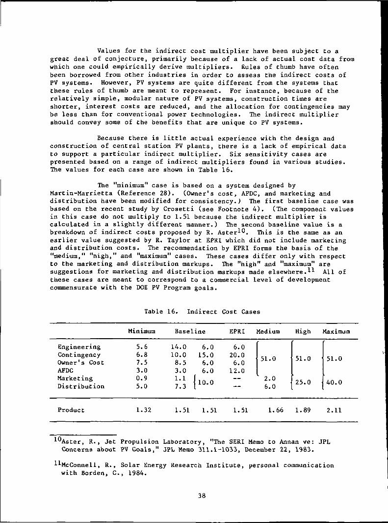
Values for the indirect cost multiplier have been subject to agreat deal of conjecture, primarily because of a lack of actual cost data fromwhich one could empirically derive multipliers. Rules of thumb have oftenbeen borrowed from other industries in order to assess the indirect costs ofPV systems. However, PV systems are quite different from the systems thatthese rules of thumb are meant to represent. For instance, because of therelatively simple, modular nature of PV systems, construction times areshorter, interest costs are reduced, and the allocation for contingencies maybe less than for conventional power technologies. The indirect multipliershould convey some of the benefits that are unique to PV systems.
Because there is little actual experience with the design andconstruction of central station PV plants, there is a lack of empirical datato support a particular indirect multiplier. Six sensitivity cases arepresented based on a range of indirect multipliers found in various studies.The values for each case are shown in Table 16.
The "minimum" case is based on a system designed byMartin-Marrietta (Reference 28). (Owner's cost, AFDC, and marketing anddistribution have been modified for consistency.) The first baseline case wasbased on the recent study by Crosetti (see Footnote 4). (The component valuesin this case do not multiply to 1.51 because the indirect multiplier iscalculated in a slightly different manner.) The second baseline value is abreakdown of indirect costs proposed by R. Aster^O. This is the same as anearlier value suggested by R. Taylor at EPRI which did not include marketingand distribution costs. The recommendation by EPRI forms the basis of the"medium," "high," and "maximum" cases. These cases differ only with respectto the marketing and distribution markups. The "high" and "maximum" aresuggestions for marketing and distribution markups made elsewhere.^ All ofthese cases are meant to correspond to a commercial level of developmentcommensurate with the DOE PV Program goals.
Table 16. Indirect Cost Cases
Product
Minimum Baseline EPRI Medium High Maximum
EngineeringContingencyOwner's CostAFDCMarketingDistribution
5.66.87.53.00.95.0
14.010.08.53.01.17.3
6.015.06.06.0
1 10.0
6.020.06.012.0
'
51.0
2.06.0
51.0
25.0 •
'
51.0
40.0
1.32 1.51 1.51 1.51 1.66 1.89 2.11
, R., jet Propulsion Laboratory, "The SERI Memo to Annan ve: JPLConcerns about PV Goals," JPL Memo 311.1-1033, December 22, 1983.
l^McConnell, R., Solar Energy Research Institute, personal communicationwith Borden, C., 1984.
38

Each case corresponds to different assumptions about the nature ofcentral station PV plants. The AFDC in the last four cases implies a 2 yearconstruction period for PV plants, and the first two cases correspond to6 month construction periods. Experience from SMUD, Carrisa, and other systeminstallations demonstrates that the modular and repetitive nature of PVsystems decreases the period between the initiation of construction and systemstartup as compared to conventional systems. ARCO reports that constructionof the 4.5 MW Carrisa facility was completed in 7 months by adopting a"factory in the field" approach to plant construction (Reference 24). The"minimum" and first baseline case assumes minimum 6 month construction periods.
The contingency markups represent different estimates of thecomplexity and the industry's familiarity with the systems. The four highestcontingency estimates are derived from the EPRI Technical Assessment Guide(see Reference 9) and are based on experience with the development ofconventional generating plants. The lower contingency estimates recognize thatPV plants are significantly simpler than other types of generating plants so thatfewer problems should be anticipated during installation. The first baselineestimate is based on contingency markups used in planning large windfarm projectsthat have relatively simple and modular technology like PV, but are moretechnically mature. This estimate is consistent with the EPRI TechnicalAssessment Guide contingency recommendations for mature technologies withdetailed design plans and cost estimates (see Reference 9). Once PV plantdesigns are fully developed, similar contingency allocations appear appropriate.
A wide range of central station marketing and distribution (M&D)costs for plant materials has been suggested. The EPRI case omits M&D costs,while the "minimum" and "baseline" cases are derived from SMUD PV project costdata and reasonable marketing scenarios (see Footnote 3). The "baseline" M&Dmarkup results in M&D costs of nearly $10 million for a 100 MW system at goalcosts. In contrast, higher M&D markups suggested elsewhere (see Footnote 9)provide Che "high" and "maximum" cases, and correspond to costs of $36 to $56million, respectively, for a 100 MW system.
There is more agreement on engineering and owner's costs. The firstbaseline engineering markup includes items other than design engineering,such as home office and construction management fees. Owner's costs include thecosts of spares, insurance, start-up, licensing, and sales taxes. Baselinevalues for these components are taken from national construction cost data andSMUD PV costs (see Footnote 4).
The effect of each of these multipliers on allowable module costs ispresented in Table 17 and Figure 15. Allowable module costs are as sensitive toindirect costs as to any other parameter. Therefore, in order to establishmeaningful goals for module research, it is necessary to have a sound assessmentof indirect costs. It is surprising that indirect costs have not been subjectto more analytical scrutiny other than the single study mentioned above.
4.6 FIXED CHARGE RATE
The fixed charge rate (FCR) is the percentage of total plant capitalconstruction costs that must be received annually by the utility over the lifeof the plant to cover the utility's capital investment in the plant. The FCR
39
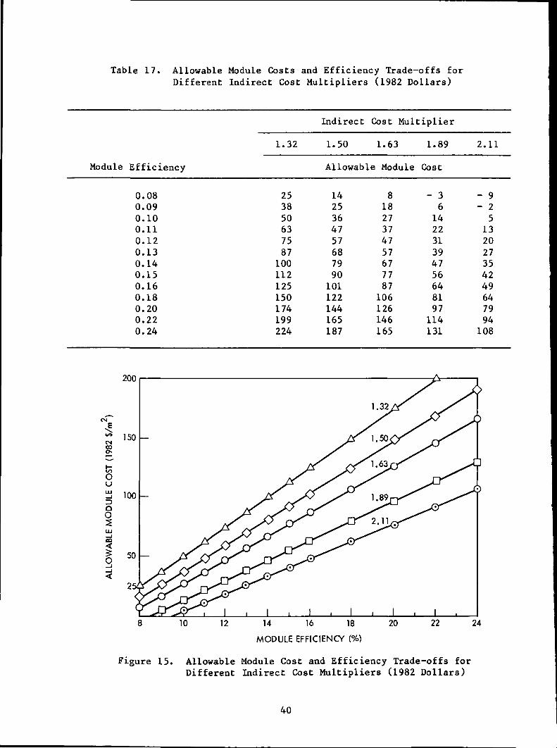
Tabl.e 17. Allowable Module Costs and Efficiency Trade-offs forDifferent Indirect Cost Multipliers (1982 Dollars)
Indirect Cost Multiplier
1.32 1.50 1.63 1.89
Module Efficiency Allowable Module Cost
8
toou
0O
<
O
10 12 14 16 18
MODULE EFFICIENCY (%)
20 22
2.11
0.080.090.100.110.120.130.140.150.160.180.200.220.24
253850637587100112125150174199224
1425364757687990101122144165187
81827374757677787106126146165
- 36142231394756648197114131
- 9- 25132027354249647994108
24
Figure 15. Allowable Module Cost and Efficiency Trade-offs forDifferent Indirect Cost Multipliers (1982 Dollars)
40

depends on interest rates, the cost of debt and equity capital, book life,income and property tax considerations, and insurance. Although the actualannual monetary requirements may vary as parameters such as taxes change, theFCR represents a levelized cost factor for recovery of the capital investment.
Because the FCR represents financial considerations that aretechnology independent, it must be used consistently when comparing twotechnologies. The 0.153 FCR used for this study is derived from the EPRITechnical Assessment Guide (see Reference 9). This value corresponds to:
(1) An inflation rate of 8.5% and a nominal discount rate of 12.5%.These rates are assumed throughout the Five-Year Research Plan.
(2) A 30 year book life for the plant, consistent with theNational Photovoltaics Program lifetime goal.
(3) All tax preferences as granted in the Economic Recovery TaxAct of 1981. EPRI recommends the inclusion of tax preferencesin economic analyses.
(4) A 15 year tax recovery period, which is the tax recoveryperiod consistent with the National Photovoltaics Programsystem lifetime goal.
A change in the FCR used for the evaluation of PV plants must beaccompanied by a change in the FCR used for the calculation of the energy costof competing technologies (i.e. the energy cost goal, EC). Because PV is acapital intensive technology, different FCR's will affect PV technology goalseven if they are used consistently in, the derivation of an energy cost goal.For instance, Table 18 shows the effects of changing the FCR from 0.153
Table 18. Allowable Module Cost and Efficiency Trade-offs forDifferent Fixed Charge Rates (1982 Dollars/m2)
Allowable Module Allowable ModuleCosts for a FCR Costs for a FCRof 0.153 and a of 0.180 and a
Module Efficiency EC of $0.15/kWh EC of $0.165/kWh
0.080.090.100.110.120.130.140.150.160.180.200.220.24
1425364757687990101122144165187
102030405060708090110130150170
41

to 0.180. Even though the FCR is changed for both PV and competing systems,resulting in a new energy cost goal of $0.165/kWh, allowable module costs arenoticeably reduced. Because the consistent use of a different FCR changes thegoals for PV technology, the value used for program planning must be chosencarefully. The value of 0.153 is used because it is consistent with othergoals and assumptions used in the Five-Year Research Plan.
4.7 OPERATION AND MAINTENANCE COST
O&M costs are annually recurring expenses for module replacement,salaries of operating personnel, module washing, and the upkeep of the grounds,structure, and electrical systems (including tracking system maintenance).Because there is little data on which to base O&M cost estimates, a wide rangeof values have been proposed. Cases involving the use of low reliabilitymodules requiring a number of replacements, inappropriate washing andmaintenance strategies, and high labor rates result in a significant change insystem energy costs. The implications for the trade-off between moduleefficiency and allowable module cost is depicted in Figure 16. High O&M costsimply significantly more challenging objectives for PV technology development.
There have been several recent attempts to estimate the O&M costsof central station PV plants12 (see References 10 and 25). Six O&Mscenarios were constructed from these estimates with annual O&M costs rangingfrom $0.19/m2 to $10.02/m2 of module area for tracking systems. Table 18shows the component costs of each scenario.
The major source of variance among these cost estimates is themodule replacement rate. This annual rate is given in parenthesis in Table 18under the associated replacement cost for each scenario. The 50 per 1000replacement rate is slightly worse than the first 6.75 years of Block I modulefield experience and may be the result of fielding new types of untestedmodules (Reference 29). (The criterion for module failure was that the moduleproduced less than 75% of its original power.) The baseline value of 4 per1000 rate is an allocation derived from engineering studies performed byR. Ross (see Reference 20). The minimum cost scenario contains negligiblemodule replacements, 1 per 100,000. In all cases, replacement costs include$0.04/m2 for the detection of modules that must be replaced (seeReference 26).
The baseline estimate for O&M costs is based on reported ARCOexperience, where the system is completely automated and no module washingoccurred (see Reference 29). Two of the scenarios include panel washing. Ifwashing is performed, then compensating changes must be made in BOS efficiencyfor consistency. Table 19 shows the effects of panel washing on allowablemodule cost for a one-axis tracking system. These results indicate that forglass encapsulated modules in remote locations, there is no benefit fromwasning.
12Soinski, Art, California Energy Commission, "Operation and MaintenanceCosts for a Conceptual 100 MW Photovoltaic Power Plant," C.E.C. InternalMemo, August 8, 1983.
42

CN
8
00
oU
Q
i
s VERY HIGH ($10.02/m )
10 12 14 16 18 20
MODULE EFFICIENCY (%)
24
Figure 16. Allowable Module Cost and Efficiency Trade-offsfor Different O&M Costs (1982 Dollars)
Grounds, structural, and electrical upkeep include estimates ofthe cost of weed control, fence maintenance, and other minor maintenanceactivities. The medium estimate is adequate for 1 to 2 weeks of labor peracre of land each year. There is no evidence of major upkeep problems forfixed flat plate systems. Tracking systems do require additional maintenance,and the additional cost is based on Martin Marrietta experience as estimatedby Black and Veatch (see Reference 10).
Baseline O&M costs provide a conservative estimate based on dataavailable to date. Table 20 shows the combinations of module cost andefficiency allowable under the various O&M scenarios for one-axis systems andthe $0.15/kWh energy cost goal.
The current formulation of O&M costs in the Five-Year Research Planholds the cost of replacement modules fixed at $90/ra and assumes a givenreplacement rate. It has been pointed out by A. Scolaro of DOE and others thatO&M costs are more appropriately modeled as a function of module costs andreplacement rates. Figure 16 and Tables 19, 20 and 21 assume that replacementmodule costs are equal to initial module costs. Table 22 gives system energycost rather than allowable module cost and efficiency trade-offs.
43

Table 19. Six O&M Cost Scenarios (1982 Dollars/m2)a
OperationsIncluding:
1 Manager2 Controllers1 Clerk
Washing(Washings /Yr)
Grounds, Structureand ElectricalUpkeep ($/Acre)
VeryHigh
0.19
YesYesYes
0.48(12)
'l.ll(1500)
High
0.15
YesYesNo
0.24(6)
0.74(1000)
Baseline
0.06
YesNoNo
0.0(0)
0.44(600)
Low
0.06
YesNoNo
0.0(0)
0.30(400)
VeryLow
0.0
NoNoNo
0.0(0)
0.15(200)
Minimum
0.0
NoNoNo
0.0(0)
0.075(100)
ModuleReplacement**(ReplacementRate)
7.04 1.44 0.60 0.18 0.06 0.04
(50/1,000) (10/1,000) (4/1,000) (1/1,000) (1/10,000) (1/100,000)
Fixed Totals 8.82 2.57 1.10 0.54 0.21
TrackingMaintenance0 1.20 0.60 0.30 0.30 0.15
Tracking Totals 10.02 3.17 1.40 0.84 0.36
0.115
0.075
0.19
aBased on a 100 MW plant size, 1:3 array to land ratio.
^Includes 0.04 for inspection and detection, plus $140/m2 for replacement.
cBlack and Veatch estimated 0.30 based on Martin Marrietta's preliminarydata on two-axis tracking failure and repair rates.
44

Table 20. Effects of Panel Washing on One-Axis Tracking AllowableModule Costs (1982 Dollars/m2)
Washings /YrSoiling EfficiencyReplacement RateOther O&M CostsBOS Efficiency
1298.5%0.0041.320.878
698%
0.0041.080.874
097%
0.0040.840.865
Module Efficiency Allowable Module Cost
0.080.100.120.140.150.160.180.200.220.24
143556778798119140161182
1637587989100121142163183
1738597990100121142162183
Table 21. Module Costs and Efficiency Trade-offs for DifferentO&M Costs with Replacement Costs Equal to OriginalModule Costs (1982 Dollars/m2)
Maximum High Baseline Low Very Low Minimum
Replacement RateBOS Efficiency
Module Efficiency
0.050.878
0.010.878
0.0040.865
0.0010.865
0.00010.865
0.000010.865
Allowable Module Cost
0.080.100.120.140.150.160.180.200.220.24
-17- 31226344155708599
62646667686106126145165
1738597990100121142162183
2142638595106127149170192
25466890100111133154176197
26487091102113134156178199
45

Table 22. Levelized System Energy Cost with Replacement CostsEqual to Original Module Costs (1982 Dollars/m2)
Replacement RateBOS Efficiency
Module Efficiency
0.120.150.180.20
0.120.150.18
0.030.120.150.18
0.100.120.150.18
0.030.080.100.12
Cost
550550550550
300300300
200200200200
90909090
30303030
Maximum
0.050.878
1.160.930.780.70
0.690.560.47
1.970.510.410.34
0.360.300.240.21
0.700.280.220.19
High
0.010.878
0.850.680.570.52
0.510.410.34
1.440.370.300.25
0.260.220.180.15
0.510.200.170.14
Baseline Low
0.0040.865
System
0.810.650.540.49
0.480.390.33
1.350.350.280.24
0.250.210.170.14
0.460.180.150.13
0.0010.865
Energy
0.780.630.530.48
0.470.380.32
1.310.340.280.23
0.240.200.160.14
0.440.180.150.12
Very Low
0.00010.865
Cost
0.770.620.520.47
0.460.370.31
1.280.330.270.23
0.230.200.160.14
0.430.170.140.12
Minimum
0.000010.865
0.770.620.520.47
0.460.370.31
1.280.330.270.23
0.230.190.160.14
0.430.170.140.12
46

SECTION 5
REFERENCES
1. U.S. Department of Energy, National Photovoltaics Program, Five-YearResearch Plan 1984-1988; Photovoltaics; Electricity from Sunlight.DOE/CE-0072, U.S. Department of Energy, Washington, D.C., May 1983.
2. Simberger, E.J., The Aerospace Corporation, letter reporting the findingsof the DOE Technical Assistance Team for the SMUD PV Project and Phase IICost Proposal to Mr. Mike Lopez, DOE, June 13, 1983.
3. Simberger, E.J., The Aerospace Corporation, letter reporting the findingsof the DOE Technical Assistance Team for the SMUD PV Project and PhaseIII Cost Proposal to Mr. Mike Lopez, DOE, June 21, 1984.
4. Sacramento Municipal Utility District, "PV Panel Bidders Conference,"Sacramento, California, October 1983.
5. Sacramento Municipal Utility District, Design and Construction of theSMUD PV1 1-MW Photovoltaic Power Plant, PV192-S01, Sacramento,California, April 1985.
6. Henry, Paul, Jet Propulsion Laboratory, "Economic Projections and FSAResearch Priorities," contained in Progress Report 21 and Proceedings ofthe 21at Project Integration Meeting, DOE/JPL 1012-88, Pasadena,California, 1983.
7. Taylor, R., "Utility Requirements for Photovoltaic Power," presented atthe 161st Meeting of the Electrochemical Society, Montreal, Canada,May 9-14, 1982.
8. Taylor, R., Electric Power Research Institute, Photovoltaic SystemsAssessment: An Integrated Perspective, EPRI AP-3176-SR, Palo Alto,California, September 1983.
9. Electric Power Research Institute, Technical Assessment Guide, EPRIP-2410-SR, Palo Alto, California, May 1982.
10. Levy, S.L., and Stoddard, L.E., Black & Veatch Engineers-Architects,Integrated Photovoltaic Central Station Conceptual Designs, EPRI AP-3264,Electric Power Research Institute, Palo Alto, California, June 1984.
11. "Coal Week Comparative Pricing Trendline, April 1984," Coal Week,Vol. 10, No. 43, October 29, 1984, McGraw-Hill Inc., New York.
12. North American Electric Reliability Council, Electric Power Supply andDemand 1984-1993, Princeton, New Jersey, 1984.
13. Jones, G. J., Sandia National Laboratories, Energy Production Trade-offsin Photovoltaic System Design, SAND82-2239, Albuquerque, New Mexico,April 1983.
47
14. Solar Energy Research Institute, Solar Radiation Energy Resource, Atlasof the United States, SERI/SP-642-1037, Golden, Colorado, October, 1981.
15. United States Bureau of the Census, Statistical Abstract of the UnitedStates, 1984, Washington, D.C., 1984.
16. Shushnar, G.J., Caldwell, J.H., Jr., Reinoehl, R.F., and Wilson, J.H.,ARCO Solar Inc., "Balance of System Costs for a 5 MW PhotovoltaicGenerating System," Chatsworth, California (presented at the IEEE/PES1985 Winter Meeting, New York, February 3-8, 1985).
17. ARCO Solar Inc., "The ARCO Solar Photovoltaic Power Plant, OneMegawatt - Hesperia, California: Technical and Organizational BackgroundInformation," Chatsworth, California, 1983.
18. ARCO Solar Inc., "The ARCO Solar Photovoltaic Power Plant, CarrisaPlain: Technical and Organizational Background Information," Chatsworth,California, 1984.
19. Hoffman, A.R., and Maag, C.R., Jet Propulsion Laboratory, PhotovoltaicModule Soiling Studies, DOE/JPL-1012-49, Pasadena, California,November 1980.
20. Ross, R.G., Jet Propulsion Laboratory, "Technical Challenges of FutureModules and Arrays," Proceeding of the 22nd Project Integration Meeting,DOE/JPL-1012-94, Pasadena, California, September 1983.
21. Otth, David H., and Ross, Ronald G., Jet Propulsion Laboratory,"Assessing Photovoltaic Module Life from Long-Term Environmental Tests,"Pasadena, California (presented in Proceedings of the 1984 Institute ofEnvironmental Sciences Conference, Orlando, Florida, April 30 toMay 3, 1984).
22. Ross, R.G., Jet Propulsion Laboratory, "Technology Developments Toward30-Year-Life Photovoltaic Modules," Pasadena, California (presented atProceedings of the 17th IEEE Photovoltaic Specialists Conference,Orlando, Florida, May 1-4, 1984).
23. Shushnar, G.J., Reinoehl, R.F., and Arnett, J.C., ARCO Solar Inc.,"Analysis of Costs for a 5 MW Photovoltaic Power Plant," R&D ExternalPub. 84-21, Chatsworth, California (prepared for 1st InternationalPhotovoltaic Science and Engineering Conference, Kobe, Japan,November 15-18, 1984).
24. Arnett, James C., and Reinoehl, Robert F., ARCO Solar Inc.,"Installations and Performance of Lugo and Carrisa Plain PhotovoltaicSystems," Woodland Hills, California (prepared for 166th ElectrochemicalSociety Meeting, New Orleans, Louisiana, October 1984).
25. Stolte, W.J., Bechtel Group Inc., Photovoltaic Balance-of-SystemAssessment, EPRI AP-2474, Electric Power Research Institute, Palo Alto,California, June 1982.
48

26. Windworks Inc., Mukwanago, Wisconsin, Advertisement, PV InternationalMagazine, June/July 1984.
27. Stolte, W.J., Bechtel Group Inc., Photovoltaic Subsystem Optimization andDesign Trade-off Study, SAND81-7013, Sandia National Laboratories,Albuquerque, New Mexico, March 1982.
28. Martin-Marrietta, Design of Photovoltaic Central Station System,SAND82-7147, SAND82-7148, SAND82-7149, Sandia National Laboratory,Albuquerque, New Mexico, February 1984.
29. Weaver, R., Lee, R., Meyer, J., and Runkle, L., Jet PropulsionLaboratory, FSA Field Test Annual Report, August 1981 - January 1984,DOE/JPL-1012-100, Pasadena, California, August 1984.
49
APPENDIX A
CURRENT STATUS OF CENTRAL STATION PV
Throughout this study, current state-of-the-art values for manyparameters have been reported. By considering current values for parameters,a picture emerges of PV's present status and the effort required to meetprogram goals.
Three cases are described. The first case leaves all economic andmeteorological values unchanged from the program values. Technical values,however, are drawn from projections of SMUD Phase 3 costs and performance (seeReference 3). By comparing the system energy costs of this case with the$0.15/kWh goal gives an indication of the aggressiveness of the national PVprogram. The other two cases include current technical values and economicand meteorological values that correspond to Southern California and theNortheast. These cases reflect some of the regional differences faced by thetechnology.
Area-related BOS costs for SMUD Phase 3 are in the region of$113/m2 to $121/m2, and power-related BOS costs range from $567/kW to$659/kW. For this analysis, area-related BOS costs are assumed to be$115/m2, and power-related BOS costs are assumed to be $600/kW. Modules areassumed to have an efficiency of 11.5% STC and a cost of $550/m2 based onARCO's sales to SMUD. BOS efficiency is set at 0.836, which is the ratereported by ARCO for their Carrisa installation after adjusting for moduledegradation of 0.65%/yr. O&M costs are set to $3.24/m2 for energy costcalculations to cover the higher module replacement costs.
For technical values corresponding to the current state of the artand recommended insolation levels, the resulting energy cost is $0.85/kWhcompared to an energy cost goal of $0.15/kWh. Using these same values and the$0.15/kWh energy cost goal, allowable modules costs are -$41/ra2 (negative)at 11.5% efficiency. As suggested earlier in Figure 1, closing this gaprequires improvement in the cost and performance of all system components, andnot just modules.
The energy cost for the Northeast case, assuming insolation forLong Island,A~l is $1.05/kWh. This reflects the region's poorerinsolation. When a competitive energy cost of $0.20/kWh is used rather thanthe $.15/kWh goal, allowable module costs become -$25/m2 at 11.5%efficiency. Higher competing energy costs in the Northeast can offset theeffects of lower insolation. If technical program goals are met, PV may evenbe competitive in the Northeast, as suggested previously in Figure 2.
Southern California is perhaps the most promising area for PV. Infact, the three largest existing central station PV plants are located in
A~^Cottingham, J.G., Brookhaven National Laboratory, "Normal Incident SolarRadiation Measurements at Upton, New York," BNL 50939, Upton, N.Y., 1979.
A-l
California (SMUD, Carrisa, and Lugo). Southern California is characterized bygood insolation and high competitive energy costs. Assuming that PVinstallations are constructed in regions of Southern California with the bestinsolation, the energy cost resulting from current technical values is$0.70/kWh. With a competitive energy cost of $0.20/kWh, allowable modulecosts are $35/m^ at 11.5% efficiency. Even if other technical parameterswere not improved, 15% modules would have to cost $84/m to make PV viablein this region. This is one region where PV may be viable before all programgoals have been met.
There has been a sharp reduction of PV costs since the Block 1module purchase in 1975. At that time, modules cost over $2100/ra2 for 6%efficient modules. ~^ Assuming the current values for other parameters,these module characteristics result in an energy cost of $4.56/kWh. Today,11.5% efficient $550/m2 modules are commercially available, and thetechnology exists to reduce module costs to $2QQ/ra; these modules couldproduce energy for $0.31/kWh, an eleven-fold reduction in cost, and only twicethe energy cost goal.
^Christiansen, E., Jet Propulsion Laboratory, "Electricity fromPhotovoltaic Solar Cells: Low-Cost Solar Array Projects," Pasadena,California, May 1981 (Presentation from 15th Annual PhotovoltaicSpecialist Conference).
A-2

APPENDIX B
DERIVATION OF THE LIFE-CYCLE MODULE DEGRADATION EFFICIENCY FACTOR
'Annual PV system output decreases overtime due to moduledegradation. In order to incorporate this effect into the derivation of alevelized system energy cost, one must consider how degradation affects therequired revenues of the plant.
The calculation of energy cost in the DOE Five Year Research Planis based on a revenue requirements methodology. This methodology requiresthat the present value of all revenues generated by the plant over itslifetime must equal its life-cycle cost.
The Five Year Research Plan and this Sensitivity Analysis statethe PV energy cost goal in terms of nominally levelized busbar energy cost(BBEC). BBEC is the one single energy price the utility could charge over theentire life of the plant and recover total life-cycle costs. In order todetermine the effect of module degradation on BBEC, one can write:
REQREV = LCC
(1 + K)1BBEC MWH.i
(1 + K)1AC.
BBEC
N
MWH (1 - d)1 =a
,AC.
where:
K = discount rate, nominal (real) if costs are in current(constant) terms.
BBEC = levelized busbar energy cost (or, alternately, requiredprice).
ACi = annual system costs in year i.
MWH^ = energy production in year i.
N = plant lifetime in years
d = annual percentage energy loss due to degradation of modules.
MWH - constant annual energy output excluding degradation.
B-l
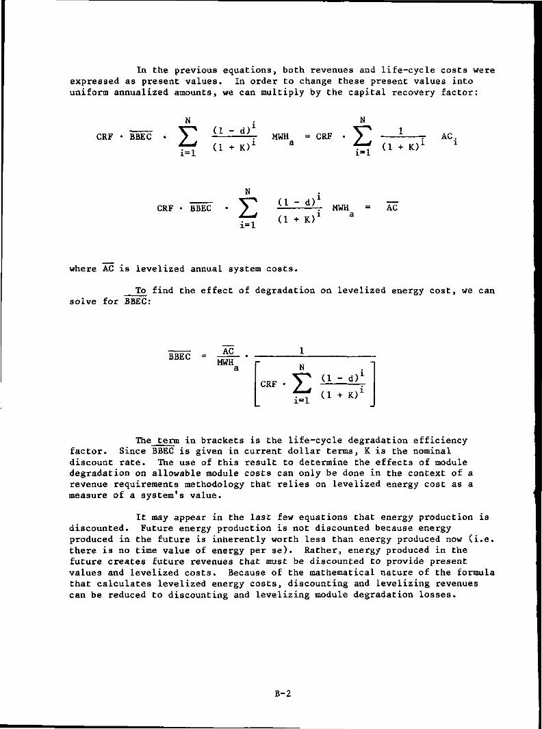
In the previous equations, both revenues and life-cycle costs wereexpressed as present values. In order to change these present values intouniform annualized amounts, we can multiply by the capital recovery factor:
CRF • BBEC • MWH = CRFa
AC.
N
CRF • BBEC MWH AC
where AC is levelized annual system costs.
To find the effect of degradation on levelized energy cost, we cansolve for BBEC:
BBECACMWH
CRF
N(1 - d)1
(1 + K)1
The term in brackets is the life-cycle degradation efficiencyfactor. Since BBEC is given in current dollar terms, K is the nominaldiscount rate. The use of this result to determine the effects of moduledegradation on allowable module costs can only be done in the context of arevenue requirements methodology that relies on levelized energy cost as ameasure of a system's value.
It may appear in the last few equations that energy production isdiscounted. Future energy production is not discounted because energyproduced in the future is inherently worth less than energy produced now (i.e.there is no time value of energy per se). Rather, energy produced in thefuture creates future revenues that must be discounted to provide presentvalues and levelized costs. Because of the mathematical nature of the formulathat calculates levelized energy costs, discounting and levelizing revenuescan be reduced to discounting and levelizing module degradation losses.
B-2
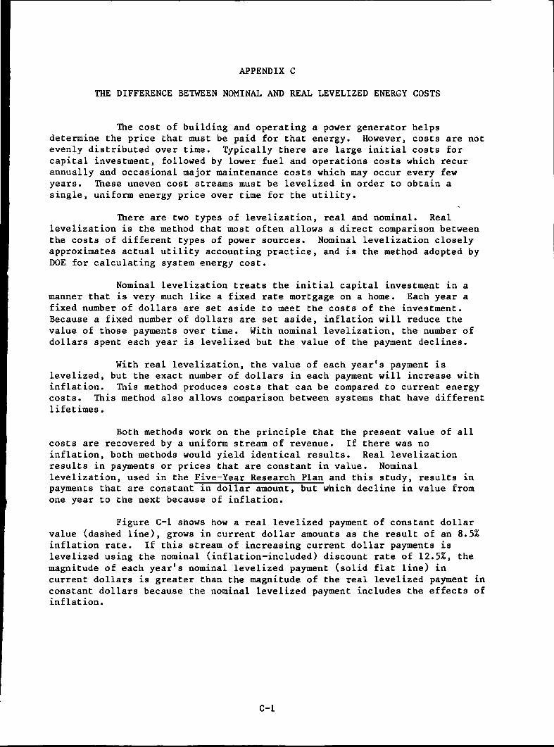
APPENDIX C
THE DIFFERENCE BETWEEN NOMINAL AND REAL LEVELIZED ENERGY COSTS
The cost of building and operating a power generator helpsdetermine the price that must be paid for that energy. However, costs are notevenly distributed over time. Typically there are large initial costs forcapital investment, followed by lower fuel and operations costs which recurannually and occasional major maintenance costs which may occur every fewyears. These uneven cost streams must be levelized in order to obtain asingle, uniform energy price over time for the utility.
There are two types of levelization, real and nominal. Reallevelization is the method that most often allows a direct comparison betweenthe costs of different types of power sources. Nominal levelization closelyapproximates actual utility accounting practice, and is the method adopted byDOE for calculating system energy cost.
Nominal levelization treats the initial capital investment in amanner that is very much like a fixed rate mortgage on a home. Each year afixed number of dollars are set aside to meet the costs of the investment.Because a fixed number of dollars are set aside, inflation will reduce thevalue of those payments over time. With nominal levelization, the number ofdollars spent each year is levelized but the value of the payment declines.
With real levelization, the value of each year's payment islevelized, but the exact number of dollars in each payment will increase withinflation. This method produces costs that can be compared to current energycosts. This method also allows comparison between systems that have differentlifetimes.
Both methods work on the principle that the present value of allcosts are recovered by a uniform stream of revenue. If there was noinflation, both methods would yield identical results. Real levelizationresults in payments or prices that are constant in value. Nominallevelization, used in the Five-Year Research Plan and this study, results inpayments that are constant in dollar amount, but which decline in value fromone year to the next because of inflation.
Figure C-l shows how a real levelized payment of constant dollarvalue (dashed line), grows in current dollar amounts as the result of an 8.5%inflation rate. If this stream of increasing current dollar payments islevelized using the nominal (inflation-included) discount rate of 12.5%, themagnitude of each year's nominal levelized payment (solid flat line) incurrent dollars is greater than the magnitude of the real levelized payment inconstant dollars because the nominal levelized payment includes the effects ofinflation.
C-l

8.5% INFLATION
REAL LEVELIZEDPAYMENTS INCURRENT DOLLARS.
Oo
10 20
YEAR
NOMINAL LEVELIZEDPAYMENTS12.5% DISCOUNT RATE
REAL LEVELIZEDPAYMENT
30
Figure C-l. The Difference Between Nominal andReal Levelized Energy Costs
C-2