1

A sequential approach to calibrate ecosystem models with multiple time

series data

Ricardo Oliveros-Ramosa,b,c, Philippe Verleyb,c and Yunne-Jai Shinb,c

a Instituto del Mar del Perú (IMARPE). Gamarra y General Valle s/n Chucuito, Callao, Perú.

b Institut de Recherche pour le Développement (IRD), UMR EME 212, Avenue Jean Monnet, CS 30171, 34203

Sète Cedex, France.

c University of Cape Town, Marine Research (MA-RE) Institute, Department of Biological Sciences, Private

Bag X3, Rondebosch 7701, South Africa.

Corresponding author: Ricardo Oliveros-Ramos: ricardo.oliveros@gmail.com

Abstract

Ecosystem approach to fisheries requires a thorough understanding of fishing

impacts on ecosystem status and processes as well as predictive tools such as

ecosystem models to provide useful information for management. The credibility of

such models is essential when used as decision making tools, and model fitting to

observed data is one major criterion to assess such credibility. However, more

attention has been given to the exploration of model behavior than to a rigorous

confrontation to observations, as the calibration of ecosystem models is

challenging in many ways. First, ecosystem models can only be simulated numerically

and are generally too complex for mathematical analysis and explicit parameter

estimation; secondly, the complex dynamics represented in ecosystem models allow

species-specific parameters to impact other species parameters through ecological

interactions; thirdly, critical data about non-commercial species are often poor;

lastly, technical aspects can be impediments to the calibration with regard to the

high computational cost potentially involved and the scarce documentation published

on fitting complex ecosystem models to data. This work highlights some issues

related to the confrontation of complex ecosystem models to data and proposes a

methodology for a sequential multi-phases calibration of ecosystem models. We first

propose two criteria to classify the parameters of a model: the model dependency

and the time variability of the parameters. Then, these criteria and the

availability of approximate initial estimates are used as decision rules to

determine which parameters need to be estimated, and their precedence order in the

sequential calibration process. The end-to-end (E2E) ecosystem model ROMS-PISCES-

OSMOSE applied to the Northern Humboldt Current Ecosystem is used as an illustrative

case study. The model is calibrated using a novel evolutionary algorithm and a

likelihood approach to fit time series data of landings, abundance indices and

catch at length distributions from 1992 to 2008.

Keywords: Stochastic models, ecosystem model, model calibration, inverse

problems, time series, ecological data, Humboldt Current Ecosystem, Peru.

2

1. Introduction

The implementation of an ecosystem approach to fisheries not only requires a

thorough understanding of the impact of fishing on ecosystem functioning and of

the ecological processes involved, but also quantitative tools such as ecosystem

models to provide useful information and predictions in support of management

decision. Yet, the use of ecosystems models as decision making tools would only be

possible if they are rigorously confronted to data by means of accurate and robust

parameter estimation methods and algorithms (Bartell 2003). In many respects, the

calibration of ecosystem models is a complex task. In particular, the dynamics

represented in ecosystem models allow species-specific parameters to have an impact

on one another through ecological interactions, which results in highly correlated

parameters. In addition, critical information and observations on non-commercial

species can be missing or poor. Furthermore, the large number of parameters and

the long duration of the simulations can be an obstacle to calibrate a model. These

diverse reasons hampered the development of flexible and generic calibration

algorithms and methodology for ecosystem models, and only sparse documentation has

been produced on fitting complex models (Bolker et al. 2013).

Given that calibration of complex ecosystem models requires a lot of data and

potentially involves a large number of parameters to be estimated, common practice

in the field has been to i) reduce the number of parameters to be estimated by

directly using estimates from other models (Marzloff et al. 2009, Lehuta et al.

2010) or available for similar species or ecosystems (Bundy 2005, Ruiz and Wolff

2011), ii) use outputs from other models as data to calibrate the model (Mackinson

and Daskalov 2007), or iii) use both strategies (Shannon et al. 2003, Guénette et

al. 2008, Friska et al. 2011, Travers-Trolet et al. 2013). These different

strategies expedite the calibration of complex models while attempting to

synthesize the maximum of available information. However, since the borrowed

parameters and outputs rely on different model assumptions, they may lead to

inaccuracy and inconsistency in parameter estimation by trying to reproduce other

models’ dynamics.”

The defect of these common practices can be overcome by implementing a multiple-

phase calibration approach (Nash and Walker-Smith 1987, Fournier et al. 2012). In

this multiple-phase approach, some parameters can be fixed at initial values

obtained from independent data, other models or expertise (Nash and Walker-Smith

1987). (Nash and Walker-Smith 1987). In particular, assigning initial guess values

for completely unknown parameters before proceeding to a full calibration of all

parameters can ease the estimation of model parameters (Nash and Walker-Smith 1987,

Fournier et al. 2012). This multiple-phase calibration approach is supported by

3

some optimization softwares, like specialized R packages or the AD Model Builder

software (Bolker et al. 2013). However, it is difficult to find in the literature

a clear roadmap or strategy to guide the users and help them to determine what

parameters should be estimated in the successive phases. It appears that the final

organization of the calibration phases is most often an empirical process and is

the result of trials and errors in the calibration procedure (Fournier 2013).

The objective of this paper is to highlight some issues related to the confrontation

of complex ecosystem models to data and propose a methodology to a sequential

calibration of ecosystem models, illustrating it with the calibration of the

ecosystem model OSMOSE (Shin and Cury 2004, Travers et al. 2009) applied to the

northern Humboldt Current Ecosystem. The first important step in a calibration is

to be able to categorize the parameters of a model. To do so, we propose two

criteria: the model dependency and the time variability of the parameters. Then,

we use these criteria and the availability of initial guess values of the parameters

to determine which parameters need to be estimated, and their precedence in the

sequential calibration process. We finally compare our sequential approach with

the results of a single step calibration of all parameters.

2. Material and methods

2.1. Parameterization and calibration

2.1.1 Types of parameters

Several classifications of model parameters can be found in the literature (e.g.

Jorgensen and Bendoricchio 2001) according to different criteria and for different

purposes. In this work, we classified the parameters according to two criteria: 1)

the dependence of the parameter on the model structural assumptions, and 2) the

time variability of the parameter in relation to its use in the model. The

categorization of the parameters is defined as follows.

Model dependency: Parameters are considered to be model-dependent when their values

can vary between models due to different model structures or assumptions. For

example, fishing mortality can be categorized as being model-dependent, because it

depends on the value of natural mortality, structural equations of the fishing

process and assumptions on the selectivity or seasonal distribution of fishing

effort. On the contrary, model-independent parameters can be estimated directly

from data and observations by simple models or theoretical relationships. For

example, parameters for the length-weight relationships or for the von Bertalanffy

growth function can be considered independent of the overarching ecosystem model

structures and assumptions.

4

Time variability: Some parameters of the model are expected to have temporal

variability at the time scale of the model and the data. For example, fish larval

mortality rates which determine the fish annual recruitment success and which are

related to environmental conditions are expected to vary annually. Other parameters

of an ecosystem model are not expected to have significant temporal variability at

the time scale of the model and the data time series, for example the parameters

of predators’ functional response.

The classification of the parameters in terms of model dependency is necessary in

order to avoid the misleading use of parameters' values which have been estimated

in other models and not directly from observations. If some parameters are fixed

at values inconsistent with the model structure currently used to fit the data,

the estimates of other parameters obtained from the calibration can be highly

uncertain and only artifacts to fit the data. This can also impede the convergence

of the objective function and lead to a calibration failure (Gaume et al. 1998,

Whitley et al. 2013).

The classification in terms of temporal variability can be more arbitrary since

many parameters (especially the ones characterizing the populations) are expected

to vary with time. The cutoff we propose for a parameter to be considered as time-

varying results from the following considerations: i) the identification of a

process leading to such time variability, ii) the existence of theoretical

assumptions about the importance of such process in the dynamics of the modeled

ecosystem, iii) the non-explicit representation of the process in the model, and

iv) the significance of the time variability compared to the time scale of the

model and the length of the data time series. Some parameters can be assumed to be

constant at shorter time scales (e.g. a few years) but can exhibit variability at

longer time scales (e.g. several decades). For example, the length at maturity for

a given species can decrease in response to heavy fishing (Shin et al. 2005), but

can be considered as constant in the model for periods short enough, or if the

variability is not considered to cause significant changes in the functioning of

the multispecies assemblage.

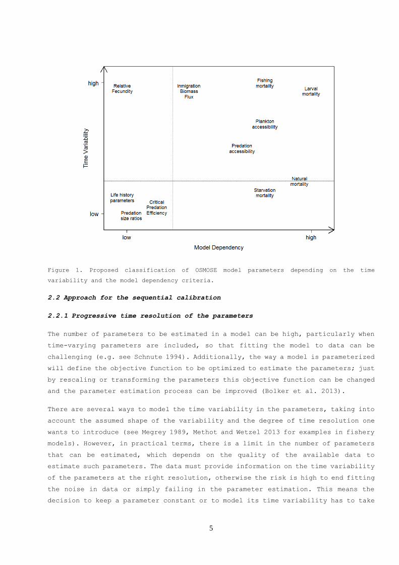
Despite the apparent dichotomous classification presented, the degree of model-

dependency and temporal variability in the parameters can vary, and a qualitative

classification of the parameters should be attempted. In the OSMOSE ecosystem

model, such classification could be proposed for the parameters characterizing

modelled multispecies fish assemblages (Figure 1; see Appendix A for details about

the parameterization of OSMOSE).

5

Figure 1. Proposed classification of OSMOSE model parameters depending on the time

variability and the model dependency criteria.

2.2 Approach for the sequential calibration

2.2.1 Progressive time resolution of the parameters

The number of parameters to be estimated in a model can be high, particularly when

time-varying parameters are included, so that fitting the model to data can be

challenging (e.g. see Schnute 1994). Additionally, the way a model is parameterized

will define the objective function to be optimized to estimate the parameters; just

by rescaling or transforming the parameters this objective function can be changed

and the parameter estimation process can be improved (Bolker et al. 2013).

There are several ways to model the time variability in the parameters, taking into

account the assumed shape of the variability and the degree of time resolution one

wants to introduce (see Megrey 1989, Methot and Wetzel 2013 for examples in fishery

models). However, in practical terms, there is a limit in the number of parameters

that can be estimated, which depends on the quality of the available data to

estimate such parameters. The data must provide information on the time variability

of the parameters at the right resolution, otherwise the risk is high to end fitting

the noise in data or simply failing in the parameter estimation. This means the

decision to keep a parameter constant or to model its time variability has to take

6

into account both the complexity of the parameter estimation and the quality of

the data used for the calibration of the model (Jorgensen and Bendoricchio 2001).

We considered different models to represent the temporal variability in the

parameters (Appendix B, Table B.1, Figure B.1), where the variability can be split

into three components: the mean value of the parameter, the high frequency

variability (seasonal or non-periodical) and the low frequency variability

(interannual). This type of parameterization allowed us to define several nested

models, i.e. models which can gradually be complexified from the simplest models'

parameterization (setting to zero the random effects in the yearly component for

the time-varying parameters) to full consideration of low and high frequency

variability. For example, the mean value of time-varying parameters over the time

series should be estimated in priority, with the interannual deviations fixed to

zero.

If the different components of time variability in a given parameter can be

introduced progressively, the final parameter estimation can be improved by

providing good initial values for the more important variability components after

preliminary calibration of simpler versions of the model. We therefore propose a

general calibration strategy that models the time-varying parameters such that the

several components of variability are independent and can be nullified by fixing

some parameters to constant values (nested models).

2.2.2. Calibration in multiple-phase

According to the parsimony principle, given models with similar accuracy, the

simplest model is the best compromise with regard to the available data. In

particular, for nested models, the complexity of a model is directly related to

the number of parameters to estimate, so the parsimony principle implies to estimate

the lowest number of parameters as possible. On the other hand, it is possible to

increase the goodness of fit of the model by increasing the number of parameters,

but this can lead to overfitting (Walter and Pronzato 1997, Bolker 2008). However,

there is no way to know a priori if all parameters will be identifiable, i.e. if

we can estimate them properly from the available data.

Based on the criteria of time variability and model dependency of the parameters,

we propose a set of rules for a hierarchical approach to select the parameters to

estimate in a model and the order at which the parameters should be estimated in

the different phases of the calibration. Also, we propose some criteria to design

nested models for taking into account time variability by using simple time series

7

models which allow to assess the usefulness of the additional temporal parameters

introduced in the model calibration.

The first rule relates to the model dependency of the parameters. Apart from the

time variability, parameters with low model dependency should be assigned values

directly from observations, simple models or from dedicated designed experiments.

On the contrary, parameters with high model dependency should always be estimated

through model calibration, because even though the theoretical meaning of the

parameters is not necessarily model-dependent, different model structures will

introduce differences in the actual meaning and value of the parameters within the

model.

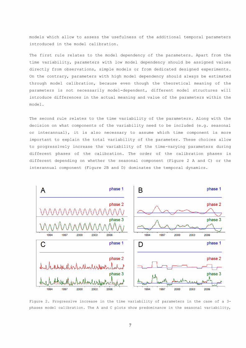
The second rule relates to the time variability of the parameters. Along with the

decision on what components of the variability need to be included (e.g. seasonal

or interannual), it is also necessary to assume which time component is more

important to explain the total variability of the parameter. These choices allow

to progressively increase the variability of the time-varying parameters during

different phases of the calibration. The order of the calibration phases is

different depending on whether the seasonal component (Figure 2 A and C) or the

interannual component (Figure 2B and D) dominates the temporal dynamics.

Figure 2. Progressive increase in the time variability of parameters in the case of a 3-

phases model calibration. The A and C plots show predominance in the seasonal variability,

8

while interannual variability is the dominant signal in plots B and D plots. The upper plots

correspond to type-A models and the lower plots to type-B models described in the appendix

B.

A third rule relates to the availability of initial estimates for the parameters

to calibrate. Even in case of model-dependency, parameters taken from other models

can be used to start the calibration. For time-varying parameters, the deviations

estimated from other models (e.g. single species models) or approximate

relationships can be used as proxies of the interannual variability if they are

estimated from the same dataset used for the current calibration. Another

alternative is to use parameters estimated from models with a similar structure,

such as previous versions (likely simpler) of the same model (e.g. a steady-state

one). It is important to note that the proxies or initial estimates will only be

used to start the calibration in a given parameter space but the parameters will

be fully estimated during the calibration, which means the final estimates can be

far from the initial values (Sonnenborg et al. 2003).

Considering all these rules together, we propose a hierarchy in the order of

parameters' estimation using a sequential calibration approach(Figure 3).

Figure3. Proposed hierarchy in the order of parameters' estimation using a sequential calibration

approach.

If we consider the initial phase of the calibration with some parameters fixed as

a way to improve the final calibration, it is possible to make changes in the

9

objective function across the different phases of the calibration (Fournier 2013).

However, by keeping constant the objective function and running a full optimization

at each phase, it is possible to analyze the improvement in the fitting process as

a result of the increased complexity of the calibration. It therefore allows to

test the usefulness of the additional parameters and to perform model selection by

detecting which parameters do not improve the data fitting.

2.3. Case model: OSMOSE for Northern Humboldt Current Ecosystem

To illustrate our calibration methodology, we applied the OSMOSE model to the

Northern Humboldt Current Ecosystem (NHCE) inhabited by the main stock of

"anchoveta" or Peruvian anchovy (Engraulis ringens). As the paper focuses on the

calibration methodology, We do not present the OSMOSE model in detail but provide

key information in Appendix A. Details of the OSMOSE model can be found in Shin

and Cury (2001, 2004) and Travers et al. (2009, 2013), and the application to the

Humboldt ecosystem is detailed by Oliveros et al. (in prep.) as well as in Appendix

A. OSMOSE is a multispecies individual-based model (IBM) which focuses on high

trophic level (HTL) species. This model assumes size-based opportunistic predation

based on the spatial co-occurrence of a predator and its prey. It represents fish

individuals grouped into schools, and models the major processes of fish life cycle

(growth, predation, natural and starvation mortalities, reproduction and migration)

and the impact of fisheries. The modeled area ranges from 20ºS to 6ºN and 93ºW to

70ºW covering the extension of the Northern Humboldt Current Ecosystem and the

Peruvian Upwelling Ecosystem (Figure 4), with 1/6º of spatial resolution. The model

explicits the life history and spatio-temporal dynamics of 9 species (1 macro-

zooplankton group, 1 crustacean, 1 cephalopod and 6 fish species), between 1992

and 2008.

10

Figure 4. Map of the modeled area. The model spatial domain is limited by the red square.

The light blue area shows the extension of the Humboldt Current Large Marine Ecosystem, and

the dark blue area the extension of the Peruvian Upwelling Ecosystem.

The NHCE exhibits a high climatic and oceanographic variability at several scales,

e.g. seasonal, interannual and decadal. The major source of interannual variability

is due to the interruption of the upwelling seasonality by the El Nino Southern

Oscillation ENSO (Alheit and Ñiquen 2004), which imposes direct effects on larval

survival and fish recruitment success (Ñiquen and Bouchon 2004). Consequently, the

fishing activity can also be highly variable, depending on the variability in the

abundance and accessibility of the main fishery resources. Due to these different

sources of temporal variability, it is thus important to model the temporal

variability in both larval mortality and fishing mortality. This variability was

modeled using time-varying parameters, which were estimated considering interannual

and seasonal variability. For both processes, we estimated the mean value and

annual deviations. The natural mortality (due to other sources of mortality not

included in the model) and plankton accessibility to fish coefficients were also

estimated.

The data used to calibrate our model were: i) biomass indices from hydro-acoustic

scientific surveys (Gutierrez et. al 2000; IMARPE 2010) and ii) total reported

landings for the main commercial species (IMARPE 2009, IMARPE 2010). Additionally,

catch-at-length data were available for anchovy and jack mackerel and catch-at-age

11

for hake. A summary of the data available, the time resolution of the information

and the period of availability is shown in Table 1. The model was confronted to

data using a likelihood approach described in Appendix A. The optimization of the

likelihood function was carried out using an evolutionary algorithm developed by

Oliveros-Ramos and Shin (submitted), since for stochastic models it is not possible

to apply derivative-based methods (see Appendix A for more details).

Table 1.Summary of data available for the calibration of the model. Years for data

availability are indicated, M (monthly) and Y (yearly) indicates the time resolution of the

data.

Catch-at-age Catch-at-length Landings Acousticindex

Euphausiids No fishing 2003 - 2008 (Y)

Anchovy (Engraulis ringens) 1992 - 2008 (M) 1992 - 2008 (M) 1992 - 2008 (Y)

Sardine (Sardine sagax) 1992 - 2008 (M) 1992 - 2008 (Y)

Jack Mackerel (Trachurus murphyi) 1992 - 2008 (Y) 1992 - 2008 (M) 1992 - 2008 (Y)

ChubMackerel (Scomber japonicus) 1992 - 2008 (M) 1992 - 2008 (Y)

Mesopelagic fish No fishing 1999 - 2008 (Y)

Red lobster (Pleuroncodes monodon) No fishing 1999 - 2008 (Y)

Jumbo squid (Dosidicus gigas) 1992 - 2008 (M) 1999 - 2008 (Y)

Peruvian hake (Merluccius gayi) 1992-2008 (Y) 1992 - 2008 (M) 1992 - 2008 (Y, trawl)

2.4. Calibration experiments

For the OSMOSE model of the Northern Humboldt Current Ecosystem (NHCE), 5 types of

parameters needed to be estimated (Table 3): i) larval mortality rates, ii) fishing

mortality rates, iii) coefficients of plankton accessibility to fish, iv) natural

mortality rates (due to other sources of mortality not explicit in OSMOSE) and, v)

fishing selectivities. Additionally, we needed to estimate the immigration flux of

the biomass of red lobster in the system. The calibration strategy proposed was

applied to our model calibration and resulted in a pre-defined order of phases for

the estimation of the parameters of the model (Table 2).

Table 2. Order of estimation of parameters in the calibration of the NHCE OSMOSE model.

Phase Parameters Remarks

1

Time-varying parameters:

- Larval mortality: mean for all species.

- Fishing mortality: mean for all species.

Non time-varying (without initial values):

- Coefficients of plankton accessibility to fish:

one for each plankton group.

- Natural mortality: all species.

- Immigration: total immigrated biomass, peak of

migration flux (red lobster).

Number of parameters estimated: 51.

- Larval and fishing mortalities are

assumed to vary with time.

- Natural mortality is assumed not to

vary with time.

12

2

Previous parameters

+ Time-varying parameters:

- Larval mortality: annual deviates (all species).

- Fishing mortality: annual deviates without proxys

(6 first years for squid).

Number of parameters estimated: 208

(including previous 51).

- Main source of variability for the

larval and fishing mortality is

assumed to be interannual.

3

Previous parameters

+ Time-varying parameters:

- Fishing mortality: annual deviates (all remaining

parameters and species).

Number of parameters estimated: 299

(including previous 208).

Main source of variability for

fishing mortality is assumed to be

interannual.

4

Previous parameters

+ Time-varying parameters:

- Larval mortality: seasonal variability (anchovy).

+ Non time-varying (with estimates):

- Selectivity parameters: anchovy, hake, jack

mackerel.

Number of parameters estimated: 307

(including previous 299).

- Seasonal variability was only

included for anchovy due to data

limitations.

- Selectivity is assumed not to vary

with time.

We considered larval and fishing mortality as time-varying parameters, and modeled

them using the functions described in appendix B (Table B.1). The immigration flux

of red lobster biomass was also treated as a time-varying parameter, but is

parameterized with two non time-varying parameters (total biomass immigrated in

the system and the time at the peak of the migration) using a "gaussian pulse" as

described in appendix B. The other parameters (natural mortality, plankton

accessibility and fishing selectivities) were considered constant during the

simulation and are ranked according to our evaluation of their model dependency

(Figure 1).

Table 3. Models used for the time variability of larval and fishing mortalities, according to the

functional forms described in Appendix B.

Species

Time-varying parameters Abundance

index quality

Time resolution of the

information

Larval

mortalities

Fishing

mortalities Catch

Catch at

age/length

1. Abundance index, stage structured fishing information.

Anchovy A.3 B.2 High Monthly Monthly

Hake A.2 B.2 High Monthly Yearly

Jack mackerel A.2 B.2 Low Monthly Yearly

2. Abundance index, aggregated fishing information.

Sardine A.2 B.2 High Monthly Not available

Chub mackerel A.2 B.2 Medium Monthly Not available

Humboldt

Squid A.2 B.2 Low Monthly Not available

13

3. Abundance index.

Red lobster A.2

Not required

High

- - Euphausiids A.2 Low

Mesopelagics A.2 Low

A steady state calibration of the NHCE-OSMOSE model was performed first,

corresponding to the initial conditions prevailing in 1992, which is the first year

of the data time series. Red lobster was not included because it immigrates in the

NHCE after 1992, during the 1997/98 El Niño event. This first calibration allowed

to provide estimates of the average value of the larval and natural mortality rates

for the modelled species. Fishing selectivity parameters were estimated only for

the species with available age or length composition data (anchovy, hake and jack

mackerel), otherwise, values from previous stock assessment were used. We used the

ratio between catch and biomass, estimated directly from data, as a proxy of the

variability of the fishing mortality rate. This ratio was split into seasonal and

interannual deviations from the average value and used as initial values for fishing

mortalities.

In order to evaluate the performance of the sequential calibration approach in the

parameter estimation, we compared it to other calibration experiments:

- We first run a one-phase calibration where all parameters were estimated at

once, while trying to keep constant the total number of function evaluations

(i.e. the number of times we run the simulation model) to make both calibrations

comparable.

- Additionally, we also run a sequential multi-phases calibration where some

parameters were fixed. Concretely, we fixed the natural and fishing mortality

variability to values reported in the literature. As in previous OSMOSE

applications (Marzloff et al. 2009, Duboz et al. 2010), natural and fishing

mortalities from the Ecopath with Ecosim model for the same system (Tam et al.

2008) were used. In this case, only larval mortalities, coefficients of fish

accessibility to plankton, the immigration flux of red lobster and average

fishing mortality were estimated.

- Finally, we run a calibration without including the annual deviates, estimating

only the long term mean of the larval mortality and the average fishing

mortality, to analyze the effect of considering time-varying parameters in the

calibration results.

In all calibration experiments, we considered commercial landings data as the most

reliable source of information, compared to estimates of species biomass derived

from scientific surveys. In consequence, more weight was given to catch data (i.e.

14

less uncertainty; CV=0.05) than to the biomass indices (CV=0.15, 0.10 for anchovy),

so the fit to catch data contributed the most to the total value of the likelihood

function we tried to optimize during the calibration process.

3. Results and discussion

3.1 Calibration in multiple-phase

As we considered commercial landings as the most reliable source of information in

the likelihood function, catch output from the NHCE-OSMOSE model should have better

fit than all the information used for the calibration. The simulated landings we

obtained are in good agreement with data, at monthly and yearly scale (Figures 5

and 6), with high correlations between observed and simulated values. The landings

of the Humboldt squid have the poorest fitting, which can be partially explained

by the lack of abundance indices and proxys for the variability in the fishing

mortality for the initial years. Landings of anchovy have the highest variability,

since fishing mortality has a strong seasonality (Oliveros-Ramos et al. 2010), with

no fishing over several months and the setting of two quotas per year. A refined

modeling of the variability of the fishing mortality for anchovy (two parameters

per year, instead of one for example) may help improve fitting to the observed

landings. Nevertheless, with the current calibration, the fit of the NHCE-OSMOSE

model to anchovy landings can be considered as satisfactory, capturing most of the

interannual variability observed for this fishery. The landings of hake are

overestimated for most of the simulated period, but the trends in variability are

properly reproduced, having the highest correlation between observed and simulated

landings among all the species. Jack mackerel and sardine are the ones presenting

the best fit, while there is a significant overestimation of the landings of chub

mackerel during 1999 and 2000. The simulated landings were produced from the

estimated fishing mortalities and our initial choice of the selectivity functions.

The fishing mortality rates for a given length or age class are highly variable

over time for all target species (Figure 7).

15

Figure 5. Fit of the NHCE-OSMOSE model to the monthly landings data for the multiple-phase reference

calibration. The grey bars represent the monthly landings predicted by the model and the dots the

observed landings, for each modelled species targeted by Peruvian fisheries.

16

Figure 6. Fit of the NHCE-OSMOSE model to the annual landings data for the multiple-phase reference

calibration. The grey and black bars represent the annual landings predicted by the model and the

observed landings, respectively, for each species with active fisheries.

17

Figure 7. Estimated average fishing mortality rates (year-1) for the most representative length or age

class observed in the fishery.

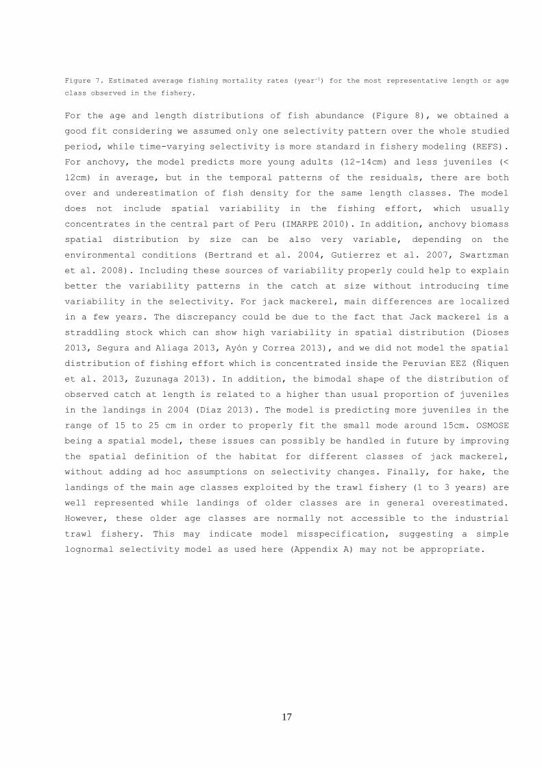
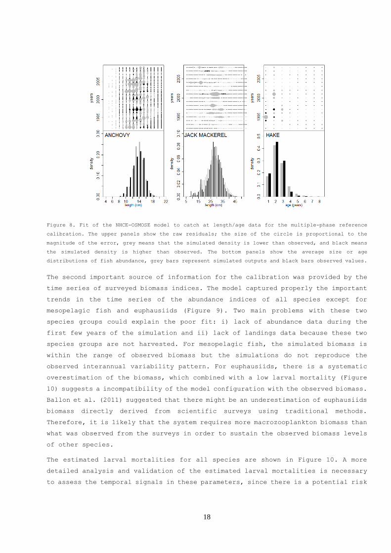
For the age and length distributions of fish abundance (Figure 8), we obtained a

good fit considering we assumed only one selectivity pattern over the whole studied

period, while time-varying selectivity is more standard in fishery modeling (REFS).

For anchovy, the model predicts more young adults (12-14cm) and less juveniles (<

12cm) in average, but in the temporal patterns of the residuals, there are both

over and underestimation of fish density for the same length classes. The model

does not include spatial variability in the fishing effort, which usually

concentrates in the central part of Peru (IMARPE 2010). In addition, anchovy biomass

spatial distribution by size can be also very variable, depending on the

environmental conditions (Bertrand et al. 2004, Gutierrez et al. 2007, Swartzman

et al. 2008). Including these sources of variability properly could help to explain

better the variability patterns in the catch at size without introducing time

variability in the selectivity. For jack mackerel, main differences are localized

in a few years. The discrepancy could be due to the fact that Jack mackerel is a

straddling stock which can show high variability in spatial distribution (Dioses

2013, Segura and Aliaga 2013, Ayón y Correa 2013), and we did not model the spatial

distribution of fishing effort which is concentrated inside the Peruvian EEZ (Ñiquen

et al. 2013, Zuzunaga 2013). In addition, the bimodal shape of the distribution of

observed catch at length is related to a higher than usual proportion of juveniles

in the landings in 2004 (Diaz 2013). The model is predicting more juveniles in the

range of 15 to 25 cm in order to properly fit the small mode around 15cm. OSMOSE

being a spatial model, these issues can possibly be handled in future by improving

the spatial definition of the habitat for different classes of jack mackerel,

without adding ad hoc assumptions on selectivity changes. Finally, for hake, the

landings of the main age classes exploited by the trawl fishery (1 to 3 years) are

well represented while landings of older classes are in general overestimated.

However, these older age classes are normally not accessible to the industrial

trawl fishery. This may indicate model misspecification, suggesting a simple

lognormal selectivity model as used here (Appendix A) may not be appropriate.

18

Figure 8. Fit of the NHCE-OSMOSE model to catch at length/age data for the multiple-phase reference

calibration. The upper panels show the raw residuals; the size of the circle is proportional to the

magnitude of the error, grey means that the simulated density is lower than observed, and black means

the simulated density is higher than observed. The bottom panels show the average size or age

distributions of fish abundance, grey bars represent simulated outputs and black bars observed values.

The second important source of information for the calibration was provided by the

time series of surveyed biomass indices. The model captured properly the important

trends in the time series of the abundance indices of all species except for

mesopelagic fish and euphausiids (Figure 9). Two main problems with these two

species groups could explain the poor fit: i) lack of abundance data during the

first few years of the simulation and ii) lack of landings data because these two

species groups are not harvested. For mesopelagic fish, the simulated biomass is

within the range of observed biomass but the simulations do not reproduce the

observed interannual variability pattern. For euphausiids, there is a systematic

overestimation of the biomass, which combined with a low larval mortality (Figure

10) suggests a incompatibility of the model configuration with the observed biomass.

Ballon et al. (2011) suggested that there might be an underestimation of euphausiids

biomass directly derived from scientific surveys using traditional methods.

Therefore, it is likely that the system requires more macrozooplankton biomass than

what was observed from the surveys in order to sustain the observed biomass levels

of other species.

The estimated larval mortalities for all species are shown in Figure 10. A more

detailed analysis and validation of the estimated larval mortalities is necessary

to assess the temporal signals in these parameters, since there is a potential risk

19

that some of its variability is an artifact to fit properly the observed biomass.

For species with length information, it is possible to better estimate the larval

mortalities since the length information helps to disentangle possible confounding

effects with other parameters like the base natural mortality (representing all

other sources of mortality not included in the model) which affects all length

classes uniformly.

Figure 9. Fit of the NHCE-OSMOSE model to the monthly survey biomass for the reference multiple-phase

calibration. The shaded area represent the 95% confidence interval for the simulated biomass,

considering the model stochasticity only. The black dots and bars represent the observed value and 95%

confidence intervals for the observations, given the CV assumed for the data errors in the calibration.

20

Figure 10. Larval mortality rates estimated by the reference multiple-phase calibration for all modelled

species.

3.2 Comparison with other calibration experiments

Since the same data has been used for all the calibration experiments, the

likelihood contribution of each source of information is comparable between models.

In particular, the first two experiments (multiple and single phases calibrations)

are directly comparable since the only difference is the strategy used for the

calibration of the same model configuration and for the same number of parameters.

The results show clearly that the multiple-phase calibration allowed to improve

the optimisation (lower AIC and negative log-likelihood; Table 4). The calibration

run with some parameters fixed from the literature, was not able to fit the landings

as well as do the other calibrations, probably because the variability in the

fishing mortality rates was fixed and these parameters are model-dependent. Also,

there is a poorest fit to the abundance indices, which can be more related to the

mis-specification of the natural mortalities. The calibration without interannual

parameters is not able to fit properly the landings nor the biomass indices, and

the interannual variability observed in the simulations come from the forcing

effect of fish habitat distribution and from the plankton dynamics (ROMS-PISCES

output forcing OSMOSE – Appendix A). Larval mortality can be strongly affected by

the environment and this parameter can have an important impact, particularly for

21

the dynamics of short lived species which depend more on the level of recruitment,

like Peruvian anchovy (Oliveros-Ramos and Peña-Tercero 2011). Since OSMOSE does

not include an explicit sub-model for such variability in eggs and larval survival,

the estimation of the interannual variability in the larval mortality was necessary.

Similar reasoning can be applied to the case of fishing mortality since the

variability in this parameter can be related not only to the availability of the

resource biomass but also to social and economical constraints.

Table4.Summary of the likelihood for the different calibration experiments of the NHCE-

OSMOSE model.

Calibrationexperiment Number

parameters AIC

Negative log-likelihood

Total Landings BiomassIndex Catch-at-

age/length

Multiple-phase 307 74807.8 37096.9 26958.7 1778.4 8333.2

Single phase 307 101030.1 50208.1 39356.8 2267.8 8543.3

Fixed parameters 207 142731.0 71158.5 57943.8 2855.9 10287.9

Without interannual

parameters 56 280353.0 140120.5 128809.7 3319.5 7985.0

Figure 11. Comparison of the likelihood components for the different calibration experiments. The

difference between the calibration experiment and the reference calibration (multiple-phase) is shown.

A negative difference means that the reference calibration fitted the data better for that particular

component. The one phase calibration is shown in grey and the calibration with fixed parameters in

black.

22

Globally, the comparative calibration experiments show that the reference

calibration (multiple-phase) fits better the landing data than do the other

calibrations (one phase and fixed parameters), except for hake where the difference

is negligible (Figure 11). The reference calibration fits better the biomass data

as well for most species. However, the reference calibration clearly performs

better in comparison to the other two calibrations. Considering the temporal

variability of the log-normal errors for the simulated landings (Figure 12), the

two calibrations with the full parameterization (one or multiple-phase) fit the

data better than the calibration with fixed parameters. Hake is the exception for

which the reference calibration produces a systematic overestimation of the

landings. The temporal patterns of the lognormal residuals of the landings are

similar for all three calibrations, which can be due to the proxys of monthly

fishing mortality variability which are common for all calibration experiments.

Nonetheless, the reference calibration produces consistently smaller residuals for

all species except for hake. In addition, for all harvested species but hake, the

total likelihood of the landings is lower in the reference multi-phases calibration

experiment.

Figure 12. Comparison of the lognormal residuals of the monthly landings for the different calibration

experiments. For each species, the multiple-phase (top), the single phase (center) and the fixed

parameters (bottom) calibration results are shown.

23

The calibration experiments were also compared with regard to the predicted species

biomass (Figure 13). The simulated trends are very similar across the calibrations

for some species (i.e. hake, sardine and chub mackerel) while more discrepancies

are present for other species. In particular, the reference calibration captured

better the interannual variability for anchovy and Humboldt squid. All the

calibrated models failed to reproduce the dynamics of the biomass of mesopelagic

fish and euphausiids. However, the behavior of the simulations for these species

shared a common pattern: steady biomass for both species, overestimation of the

euphausiids biomass and average biomass of mesopelagic fish in the range of observed

biomass.

Figure 13. Comparison of the fit of the NHCE-OSMOSE model to surveyed biomass in the different

calibration experiments. The shaded area represent the 95% confidence interval for the simulated biomass

and considering the model stochasticity only. The black dots and bars represent the observed value and

95% confidence intervals for the observations, given the CV assumed for the data in the calibration.

The calibration fixing parameters from other models estimates (green) is compared to the one phase

calibration (red). The reference calibration in multiple-phase (blue) is also shown.

For all our experiments, we have used the standard information used in fishery

models (landings, abundance indices, catch at age or length). Since ecosystem

models can provide more outputs to be confronted to data (e.g. diets, size spectrum,

and other community indicators), the availability and use of these additional

information could help selecting the more appropriate parameterization among

24

different alternatives. On the other hand, if this type of data is not available,

this could direct new objectives in data collection (Rose 2012) which can lead to

important and necessary improvements of ecosystem models in general.

4. Conclusions and perspectives

Using a dedicated global search optimization method (Oliveros-Ramos and Shin, in

prep.), we proposed a sequential multi-phases calibration approach which allowed

to improve significantly the estimation of the model parameters and to lead to a

better agreement between the model and the data. Our main objective was to provide

guidelines to improve the calibration of ecosystem models. We focused on model

dependency and time variability to categorize the parameters since these are two

criteria which are usually considered to reduce the number of parameters to

estimate. This preliminary parameters’ classification can lead to fixing parameter

values from other models or species/ecosystems or to ignoring time variability in

the parameters (Lehuta et al 2013). However, in the present study, we have not

considered other useful criteria such as sensitivity analysis, which has been used

to reduce the number of parameters to be estimated (Megrey et al. 2007, Dueri et

al. 2012, Lehuta et al 2013). Additionally, a successful calibration does not mean

that a model is reliable (Gaume et al. 1998), and a proper validation is always

required, eventually providing information to improve the model and to revise the

calibration (Walter and Pronzato 1997, Jorgensen and Bendoricchio 2001).

Acknowledgements

The authors were partly funded through the French project EMIBIOS (FRB, contract

no. APP-SCEN-2010-II). ROR was supported by an individual doctoral research grant

(BSTD) from the "Support and training of scientific communities of the South"

Department of IRD, managed by Egide. We thank the staff of IMARPE for collecting

and processing all the data used in this paper, and Coleen Moloney and Arnaud

Bertrand for their support and advice during the development of this research. All

the calibration experiments were performed with the IFREMER-CAPARMOR HPC 600

facilities. This work is a contribution from the Cooperation agreement between the

Instituto del Mar del Peru (IMARPE) and the Institut de Recherche pour le

Developpement (IRD), through the LMI DISCOH. The editors of the special volume

dedicated to Bernard Megrey are warmly thanked for their initiative.

References.

25

Alheit J., Ñiquen M., 2004. Regime shifts in the Humboldt Current ecosystem. Progress in

Oceanography 60:201–222.

Ayón P. and Correa J., 2013. Spatial and temporal variability of Jack mackerel Trachurus

murphyi larvae in Peru between 1966 –2010. Rev. peru. biol. 20(1):083- 086.

Bäck T., Schewefel H.-P., 1993. An Overview of Evolutionary Algorithms for parameter

optimization. Evolutionary Computation 1:1-23.

Ballon M., Bertrand A., Lebourges D. A., Gutierrez M., Ayon P., Grados D., Gerlotto F.,

2011. Is there enough zooplankton to feed forage fish populations off Peru? An acoustic

(positive) answer. Progress in Oceanography 91 (4):360-381.

Bartell S.M., 2003. Effective use of ecological modeling in management: The toolkit

concept. In Dale V (editor).Ecological modeling for resource management, Springer Verlag.

Bakun A. and Parrish R., 1982. Turbulence, transport, and fish in California and Peru

currents. Calcofi Rep. Vol. xxiii. 99-112.

Bertrand A., Segura M., Gutiérrez M., Vásquez L., 2004. From small-scale habitat loopholes

to decadal cycles: a habitat-based hypothesis explaining fluctuation in pelagic fish

populations off Peru. Fish and Fisheries 5:296–316.

Bolker B.M., 2008. Ecological models and Data in R. Princeton University Press. 408pp.

Bolker B.M., Gardner B., Maunder M., Berg C.W. , Brooks M., Comita L., Crone E., Cubaynes

S., Davies T., de Valpine P., Ford J., Gimenez O., Kéry M., Kim E.J., Lennert-Cody C.,

Magnusson A., Martell S., Nash J., Nielsen A., Regetz J., Skaug H., Zipkin E., 2013.

Strategies for fitting nonlinear ecological models in R, AD Model Builder, and BUGS. Methods

in Ecology and Evolution 4: 501–512.

Bundy A., 2005. Structure and functioning of the eastern Scotian Shelf ecosystem before

and after the collapse of ground fish stocks in the early 1990s. Canadian Journal Of

Fisheries And Aquatic Sciences 62:1453-1473.

Diaz E., 2013. Estimation of growth parameters of Jack mackerel Trachurus murphyi caught

in Peru from length frequency analysis. Rev. peru. biol. 20(1):061- 066.

Dioses T., 2013. Abundance and distribution patterns of Jack mackerel Trachurus murphyi

in Peru. Rev. peru. biol. 20(1):067- 074.

Duboz R., Versmisse D., Travers M., Ramat E., Shin Y.-J., 2010. Application of an

evolutionary algorithm to the inverse parameter estimation of an individual-based model.

Ecological Modelling 221(5):840-849.

Dueri S., Faugeras B., Maury O., 2012. Modelling the skipjack tuna dynamics in the Indian

Ocean with APECOSM-E – Part 2: Parameter estimation and sensitivity analysis. Ecological

Modelling 245:55-64.

Echevin V., Goubanova K., Dewitte B., Belmadani A., 2012. Sensitivity of the Humboldt

Current system to global warming: a downscaling experiment of the IPSL-CM4 model, Climate

Dynamics. doi:10.1007/s00382-011-1085-2.

Fournier D.A., Skaug H.J., Ancheta J., Ianelli J., Magnusson A., Maunder M.N., Nielsen

A., Sibert J., 2012. AD Model Builder: using automatic differentiation for statistical

inference of highly parameterized complex nonlinear models. Optimization Methods and

Software, 27:2, 233-249, DOI: 10.1080/10556788.2011.597854.

Fournier D.A., 2013. An introduction to AD Model Builder for use in Nonlinear Modeling

and Statistics. ADMB Foundation, Honolulu. 212pp.

Friska M.G., Miller T.J., Latour R.J., Martell S.J.D., 2011. Assessing biomass gains from

marsh restoration in Delaware Bay using Ecopath with Ecosim. Ecological Modelling 222:190–

200.

Gaume E., Villeneuve J.-P., Desbordes M., 1998. Uncertainty assessment and analysis of

the calibrated parameter values of an urban storm water quality model. Journal of Hydrology

210: 38–50.

Guénette S., Christensen V., Pauly D., 2008. Trophic modelling of the Peruvian upwelling

ecosystem: Towards reconciliation of multiple datasets. Progress in Oceanography 79: 326–

335.

26

Gutiérrez M. et al., 2000. Estimados de biomasa hidroacústica de los cuatro principales

recursos pelágicos en el mar peruano durante 1983 -2000. Bol. Inst. Mar Perú. Vol. 19, n°1-

2, pp. 136-156.

Gutiérrez M., Swartzman G., Bertrand A., Bertrand S., 2007. Anchovy (Engraulis ringens)

and sardine (Sardinops sagax) spatial dynamics and aggregation patterns in the Humboldt

Current ecosystem, Peru, from 1983–2003. Fish. Oceanogr. 16:2, 155–168.

IMARPE, 2009. Informe sobre la tercera reunión de expertos en dinámica de evaluación de

la merluza peruana. Bol. Inst. Mar. Perú – Callao. Bol. Inst. Mar Perú 24(1-2).

IMARPE, 2010. Informe sobre la quinta reunión de expertos en dinámica de población de la

anchoveta peruana. Bol. Inst. Mar. Perú – Callao. Bol. Inst. Mar Perú 23(1-2).

Jones G., 1998. Genetic and evolutionary algorithms. Encyclopedia of Computational

Chemistry. John Wiley and Sons.

Jorgensen S.E. and Bendoricchio G., 2001. Fundamentals of Ecological Modelling. Third

Edition. Elsevier. 530pp.

Lehuta S., Mahévas S., Petitgas, P., Pelletier D., 2010. Combining sensitivity

and uncertainty analysis to evaluate the impact of management measures with ISIS–

Fish: marine protected areas for the Bay of Biscay anchovy (Engraulis encrasicolus)

fishery. ICES J. Mar. Sci. 67, 1063–1075.

Lehuta S., Petitgas P., Mahévas S., Huret M., Vermard Y., Uriarte A., Record N.R., 2013.

Selection and validation of a complex fishery model using an uncertainty hierarchy.

Fisheries Research 143:57– 66.

Mackinson S., and Daskalov G., 2007. An ecosystem model of the North Sea for use in

research supporting the ecosystem approach to fisheries management: description and

parameterisation [online]. (CEFAS, Lowestoft.) Available from

www.cefas.co.uk/publications/techrep/tech142.pdf.

Marzloff M., Shin Y.-J., Tam J., Travers M., Bertrand A., 2009. Trophic structure of the

Peruvian marine ecosystem in 2000–2006: Insights on the effects of management scenarios for

the hake fishery using the IBM trophic model Osmose. Journal of Marine Systems 75: 290-304.

Maunder M.N. and Deriso R.B., 2003. Estimation of recruitment in catch-at-age models.

Can. J. Fish. Aquat. Sci.60: 1204–1216.

Megrey B.A., 1989. A Review and Comparison of Age-Structured Stock Assessment Models from

Theoretical and Applied Points of View. NWAFC Processed Report 88-21. 124pp.

Megrey B.A., Rose K.A, Klumb R.A, Hay D.E, Werner F.E, Eslinger D.L, Smith S.L., 2007. A

bioenergetics-based population dynamics model of Pacific herring (Clupea harengus pallasi)

coupled to a lower trophic level nutrient–phytoplankton–zooplankton model: Description,

calibration, and sensitivity analysis. Ecological Modelling 202:144–164.

Methot R.D. Jr. and Wetzel C.R., 2013. Stock synthesis: A biological and statistical

framework for fish stock assessment and fishery management. Fisheries Research 142:

86–99.

Nash J.C. and Walker-Smith M., 1987. Nonlinear Parameter Estimation: an Integrated System

in BASIC. Marcel Dekker, New York. 493pp.

Ñiquen M., Bouchon M., Ulloa D., Medina A., 2013. Analysis of the Jack mackerel Trachurus

murphyi fishery in Peru. Rev. peru. biol. 20(1):097-106.

Ñiquen M, Bouchon M., 2004. Impact of El Niño event on pelagic fisheries in Peruvian

waters. Deep-Sea Research II 51:563-574.

Oliveros-Ramos R., Guevara-Carrasco R., Simmonds J., Cirske J., Gerlotto F., Peña-Tercero

C., Castillo R., Tam J., 2010. Modelo de evaluación integrada del stock norte-centro de la

anchoveta peruana Engraulis ringens. BolInst mar Perú 25(1-2):49-55.

Oliveros-Ramos R., Peña-Tercero C., 2011. Modeling and analysis of the recruitment of

Peruvian anchovy (Engraulis ringens) between 1961 and 2009. Ciencias Marinas 37(4B):659-

674.

Oliveros-Ramos R. and Shin Y.-J. Unpublished results. calibraR: an R package for the

calibration of individual based models. (Submitted to Methods in Ecology and Evolution).

27

Oliveros-Ramos et al. Unpublished results. An end-to-end model ROMS-PISCES-OSMOSE of the

northern Humboldt Current Ecosystem. In preparation.

Oliveros-Ramos et al. Unpublished results. Pattern oriented validation of habitat

distribution models: application to the potential habitat of main small pelagics in the

Humboldt Current Ecosystem. In preparation.

Rose K., 2012. End-to-end models for marine ecosystems: Are we on the precipice of a

significant advance or just putting lipstick on a pig? Scientia Marina 76:195-201.

Ruiz D.J, Wolff M., 2011. The Bolivar Channel Ecosystem of the Galapagos Marine Reserve:

Energy flow structure and role of keystone groups. Journal of Sea Research 66 (2011) 123–

134.

Schnute J.T., 1994. A general framework for developing sequential fisheries models. Can.

J. Fish. Aquat. Sci. 51:1676-1688.

Segura M. and Aliaga A., 2013. Acoustic biomass and distribution of Jack mackerel

Trachurus murphyi in Peru. Rev. peru. biol. 20(1):087- 096.

Shannon L.J., Moloney C.L., Jarre A., Field J.G., 2003. Trophic flows in the southern

Benguela during the 1980s and 1990s. Journal of Marine Systems 39:83 – 116.

Shin Y.-J., Cury P., 2001. Exploring fish community dynamics through size-dependent

trophic interactions using a spatialized individual-based model. Aquatic Living Resources,

14(2): 65-80.

Shin Y.-J., Cury P., 2004. Using an individual-based model of fish assemblages to study

the response of size spectra to changes in fishing. Canadian Journal of Fisheries and Aquatic

Sciences, 61: 414-431.

Shin Y.-J., Rochet M.-J., Jennings S., Field J., Gislason H., 2005. Using size-based

indicators to evaluate the ecosystem effects of fishing. ICES Journal of marine Science

62(3): 394-396.

Sonnenborg T.O., Christensen B.S.B., Nyegaard P., Henriksen H.J., Refsgaard C., 2003.

Transient modeling of regional groundwater flow using parameter estimates from steady-state

automatic calibration. J. Hydrol. (Amsterdam) 273:188–204.

Swartzman G., Bertrand A., Gutiérrez M., Bertrand S., Vasquez L., 2008. The relationship

of anchovy and sardine to water masses in the Peruvian Humboldt Current System from 1983 to

2005. Progress in Oceanography 79 (2008) 228–237.

Tam J., Taylor M.H., Blaskovic V., Espinoza P., Ballón M., Díaz E., Wosnitza-Mendo C.,

Argüelles J., Purca S., Ayón P. et al., 2008. Trophic modeling of the Northern Humboldt

Current Ecosystem. Part I: Comparing trophic linkages under La Niña and El Niño conditions.

Progress In Oceanography 79(2-4):352-365.

Travers M., Shin, Y.-J., Jennings, S., Machu, E., Huggett, J.A., Field, J.G., Cury, P.M.,

2009. Two-way coupling versus one-way forncing of plankton and fish models to predict

ecosystem changes in the Benguela. Ecological modelling 220: 3089-3099.

Travers-Trolet M., Y.-J. Shin & J.G. Field., 2013. An end-to-end coupled model ROMS-

N2P2Z2D2-OSMOSE of the southern Benguela foodweb: parameterisation, calibration and pattern-

oriented validation, African Journal of Marine Science, 36:1, 11-29,

DOI:10.2989/1814232X.2014.883326

Walter E. and Pronzato L., 1997. Identification of parametric models from Experimental

data. Springer Masson. 413pp.

Whitley R., Taylor D., Macinnis-Ng C., Zeppel M., Yunusa I., O’Grady A., Froend R., Medlyn

B. and Eamus D., 2013. Developing an empirical model of canopy waterflux describing the

common response of transpiration to solar radiation and VPD across five contrasting woodlands

and forests. Hydrol. Process. 27: 1133–1146.

Zuzunaga J., 2013. Conservation and fishery management regulations of Jack mackerel

Trachurus murphyi in Peru. Rev. peru. biol. 20(1):107 - 113.

28

Appendix A. Description of the OSMOSE model for the Northern Humboldt

Current Ecosystem.

For the NHCE OSMOSE model, we considered 13 species (Table A.1), 9 being explicitly

modeled in OSMOSE (1 macrozooplankton, 1 crustacean, 1 cephalopod and 6 fish

species) and 4 plankton groups being represented in the ROMS-PISCES model. Total

plankton biomass and average distribution from ROMS-PISCES model during the study

period is shown in Figure A.1. Using Generalized Additive Models, we built maps

for the spatial distribution of the species explicitly modeled in OSMOSE (Oliveros-

Ramos et al. in prep. b). Providing the probability of occurrence of a species

given some environmental predictors (temperature, salinity, chlorophyll-a, oxygen

and bathymetry), annual maps were produced with seasonal time resolution for all

species (4 maps per year) except euphausiids, for which monthly resolution (12 maps

per year) was used. The average spatial distributions over the modeled period for

each species are shown in Figure A.2.

Table A.1. Species or functional groups considered in the NHCE OSMOSE model. The main

representative species of the functional groups are marked with an asterisk.

Group Species or

functional groups Scientific name Model

Phytoplankton Nanophytoplankton ROMS-PISCES

Diatoms ROMS-PISCES

Zooplankton

Microzooplankton ROMS-PISCES

Mesozooplankton ROMS-PISCES

Euphausiids Euphausia mucronata* OSMOSE

Small pelagics Anchovy Engraulis ringens OSMOSE

Sardine Sardinops sagax OSMOSE

Medium pelagics Jack Mackerel Trachurus murphyi OSMOSE

Chub Mackerel Scomber japonicus OSMOSE

Other pelagics

Mesopelagics Vinciguerria sp.* OSMOSE

Red lobster Pleuroncodes monodon OSMOSE

Humboldt squid Dosidicus gigas OSMOSE

Demersal Peruvian hake Merluccius gayi peruanus OSMOSE

To compare the model biomass with the estimated by scientific surveys, we estimate

a catchability coefficient q from the average ratio between the distribution area

and the area covered by the scientific surveys. This value was close to 1 for five

species with a more coastal distribution and a good coverage of the surveys

(anchovy, sardine, chub mackerel, red lobster and hake), while lower than 1 for

four species (jack mackerel, mesopelagics, euphausiids and Humboldt squid).

29

We considered a constant selectivity over the whole model period, but used different

models (logistic, normal and lognormal) for each species. A logistic selectivity

was used for sardine, chub mackerel and Humboldt squid; a normal selectivity for

anchovy and jack mackerel; and a log-normal selectivity for hake. All selectivities

were length-based but for hake we used an age-based selectivity.

Figure A.1. Summary of the LTL biomass simulated by ROMS-PISCES model and forcing OSMOSE.

Average spatial distribution for nanophytoplankton (A), diatoms (B), microzooplankton (C)

and mesozooplankton (D) (red is high, blue is low, following the light visible spectrum).

Simulated temporal dynamics of the total biomass (millions of tonnes) of the four plankton

groups (E) is also shown.

30

Figure A.2. Average probability distribution maps for OSMOSE species as predicted by

generalized additive models (Oliveros-Ramos et al. in prep.). Probability distributions are

constructed from the GAM outputs (red is high, blue is low, following the light visible

spectrum).

The objective function for the calibration was a penalized negative log-likelihood

function. For the likelihoods, we considered three main components: i) the errors

in the biomass indices (e.g. acoustic, trawl), ii) the errors in the landings and

iii) the errors in the proportions of catch-at-length or catch-at-age. A log-normal

distribution was assumed for the biomass indices and landings errors, while for

the age and length composition data the likelihood proposed by Maunder and Deriso

(2003) was used. We also added penalties to constrain the variability in the time-

varying parameters, in order to avoid overfitting. A full description of the

components of the objective function is providedin Table A.2.

Table A.2. Components of the objective function.

31

Likelihood/Penalty

component

Equations of the likelihoods Remarks

Likelihoods

Biomass Index

𝐿1 =∑𝜆𝑠,1∑log(𝑞𝑠𝐵𝑠(𝑡) + 0.01

𝐼𝑠(𝑡) + 0.01)

2

𝑡𝑠

𝜆𝑠,1 = 22.2 for all

species s but anchovy

𝜆𝑎𝑛𝑐ℎ𝑜𝑣𝑦,1 = 50

Monthly Landings

𝐿2 =∑𝜆𝑠,2∑log(𝑌𝑠(𝑡) + 0.01

�̂�𝑠(𝑡) + 0.01)

2

𝑡𝑠

𝜆𝑠,2 = 200 for all

exploited species s

Catch-at-length

𝐿3 = ∑𝑇𝑠,𝑙 ∑∑−ln [exp(−(𝑃𝑠

𝑙(𝑦) − �̂�𝑠𝑙(𝑦))2

2σs2

) + 10−3]

𝑙

𝑇

𝑦=1𝑠

𝑇𝑎𝑛𝑐ℎ𝑜𝑣𝑦,𝑙 = 5

𝑇𝑗𝑎𝑐𝑘_𝑚𝑎𝑐𝑘𝑒𝑟𝑒𝑙,𝑙 = 10

Catch-at-age

𝐿4 =∑𝑇𝑠,𝑎∑∑−ln [exp(−(𝑃𝑠

𝑎(𝑦) − �̂�𝑠𝑎(𝑦))2

2σs2

) + 10−3]

𝑎

𝑇

𝑦=1𝑠

𝑇ℎ𝑎𝑘𝑒,𝑎 = 10

Penalties

Larval mortality annual

deviates 𝑃1 =∑𝑝𝑠,3

𝑠

∑Λ𝑦

𝑇

𝑦=1

𝑝𝑠,3 = 2 for all species

but

𝑝𝑎𝑛𝑐ℎ𝑜𝑣𝑦,3 = 1, 𝑝𝑠𝑞𝑢𝑖𝑑,3 = 8,

𝑝𝑒𝑢𝑝ℎ𝑎𝑢𝑠𝑖𝑖𝑑,3 = 4.

Natural mortality

monthly deviations from

proxy

𝑃2 =∑𝑝𝑠,4𝑠

∑𝑚(𝑡)

𝑇

𝑦=1

𝑝𝑠,4 = 0.5 for all

species

Objective function

𝐿 =∑𝐿𝑖

5

𝑖=1

+∑𝑃𝑖

2

𝑖=1

The optimization problem related to minimizing the negative log-likelihood L was

solved using an evolutionary algorithm developed by Oliveros-Ramos and Shin

(submitted), since for stochastic models it is not possible to apply derivative-

based methods (e.g. gradient descent or quasi-Newton methods). Evolutionary

algorithms (EAs), which are meta-heuristic optimization methods inspired by

Darwin’s theory of evolution (Jones 1998), have shown their capability to yield

good approximate solutions in cases of complicated multimodal, discontinuous, non-

differentiable, or even noisy or moving response surfaces of optimization problems

(Bäck and Schewefel 1993). They prove to be useful alternatives for the calibration

of stochastic and complex non-linear models. In this EA, different parameter

combinations are tested as possible solutions to minimize the L function. At each

generation (i.e iteration of the optimization process), the algorithm calculates

an "optimal parent" which results from the recombination of the parameter sets

which provide the best solution for each objective (e.g. likelihood for biomass,

yield, age/length structure). The optimal parent is then used to produce a new set

of parameter combinations. To calculate this optimal parent, potential solutions

are weighted according to the variability of each parameter across generations,

32

using the coefficient of variation to take into account differences in the order

of magnitude between different parameters.

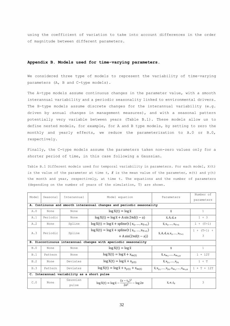
Appendix B. Models used for time-varying parameters.

We considered three type of models to represent the variability of time-varying

parameters (A, B and C-type models).

The A-type models assume continuous changes in the parameter value, with a smooth

interannual variability and a periodic seasonality linked to environmental drivers.

The B-type models assume discrete changes for the interannual variability (e.g.

driven by annual changes in management measures), and with a seasonal pattern

potentially very variable between years (Table B.1). These models allow us to

define nested models, for example, for A and B type models, by setting to zero the

monthly and yearly effects, we reduce the parameterization to A.0 or B.0,

respectively.

Finally, the C-type models assume the parameters taken non-zero values only for a

shorter period of time, in this case following a Gaussian.

Table B.1 Different models used for temporal variability in parameters. For each model, X(t)

is the value of the parameter at time t, �̅� is the mean value of the parameter, m(t) and y(t)

the month and year, respectively, at time t. The equations and the number of parameters

(depending on the number of years of the simulation, T) are shown.

Model Seasonal Interannual Model equation Parameters Number of

parameters

A. Continuous and smooth interannual changes and periodic seasonality

A.0 None None log X(t) = log x̅ x̅ 1

A.1 Periodic None log X(t) = log x̅ + A sin 2πd(t − a) x̅, A, d, a 1 + 3

A.2 None Spline log X(t) = log x̅ + spline(t|x1, … , xT+1) x̅, x1, … , xT+1 1 + (T+1)

A.3 Periodic Spline log X(t) = log x̅ + spline(t|x1, … , xT+1)

+ A sin(2πd(t − a)) x̅, A, d, a, x1, … , xT+1

1 + (T+1) +

3

B. Discontinuous interannual changes with aperiodic seasonality

B.0 None None log X(t) = log x̅ x̅ 1

B.1 Pattern None log X(t) = log x̅ + xm(t) x̅, xm1,… , xm12T

1 + 12T

B.2 None Deviates log X(t) = log x̅ + xy(t) x̅, xy1 , … , xyT 1 + T

B.3 Pattern Deviates log X(t) = log x̅ + xy(t) + xm(t) x̅, xy1 , … , xyT , xm1, … , xm12T

1 + T + 12T

C. Interannual variability as a short pulse

C.0 None Gaussian

pulse log X(t) = log x̅ −

(x − t0)2

2σ2− log2σ x̅, 𝜎, 𝑡0 3

33

Figure B.1. Examples of the different models used for time-varying parameters.