a serialization based partial decoupling approach for ... · a serialization based partial...
TRANSCRIPT
A serialization based partial decoupling approach for
multidisciplinary design optimization of complex systems
Wenqiang Yuan1, Yusheng Liu1*, Hongwei Wang2, Xiaoping Ye3
(1. State Key Lab. of CAD&CG, Zhejiang University, Hangzhou, China, 310058)
(2. School of Engineering, University of Portsmouth, Portsmouth, UK, PO1 3DJ)
(3. Institute of Lishui, Lishui, 323000)
Abstract:The optimization for multidisciplinary engineering systems is highly complicated,
which involves the decomposing of a system into several individual disciplinary subsystems for
obtaining optimal solutions. Managing the coupling between subsystems remains a great challenge
for global optimization as existing methods involve inefficient iterative solving processes and thus
have higher time cost. Some strategies such as discipline reorder, coupling suspension and
coupling ignoring, can to some extent reduce the execution cost. However, these approaches also
have some drawbacks such as low search efficiency because of overwhelmed constraints at the
system level and huge iterative computational cost for maintaining system consistency. More
important issues should be considered including maintaining the whole system compatibility when
achieving minimization/maximization of objective functions, ensuring a balance of running times
between the solving processes for different disciplines and determining which discipline should be
resolved to achieve a better performance. To overcome the above drawbacks, a Serialization based
Partial Decoupling (SPD) approach is proposed in this study, which consists of three main steps.
Firstly, different disciplines are clustered into some subsystems by analyzing the interdisciplinary
sensitivities. Then, for each subsystem a serialization process is proposed to ensure no coupling
loops exist and the subsystem can be solved with no iteration, which can reduce the time cost for
solving the disciplinary problem to a large degree. Finally, a local optimization model is
constructed for each subsystem to maintain the scale of the global optimizer and ensure mutual
independence and parallel processing. The proposed three-layer framework ensures the feasibility
of solving for each subsystem and improves the efficiency of optimization execution. Several
experiments have been conducted to demonstrate the effectiveness and feasibility of the proposed
approach.
Keywords: Serialization; Partial decoupling; Clustering analysis; Serializable solving; Local
optimization; MDO
1. Introduction
The design problems in modern engineering
systems generally have a large scale and
involve many factors from a number of
domains. Therefore, this type of problem is
often logically divided into several disciplines
by researchers and engineers, each of which is
derived from one or more major domains [1-3].
An imperative issue in the case of
multidisciplinary design and optimization is to
address the unavoidable couplings among
these disciplines [4-6]. Thus, the complex
couplings and dependencies should be
considered to get the optimal solutions during
the process of complex system design [7-9].
With the requirements of high computational
precision for highly complex design problems,
the traditional theories of complex system
design have evident limitations as they have
no consideration of interdisciplinary couplings
* Corresponding author: State Key Lab. of CAD&CG,
have shown limitations. Multidisciplinary
Design Optimization (MDO) [10-12] is a hot
research field in recent years in which the
interdisciplinary couplings are considered to
construct high-fidelity models of complex
problems during the early analysis phase
[13-15]. However, how to solve MDO
problems efficiently is still a great challenge.
A lot of research has been conducted to
develop efficient and feasible decoupling
strategies for MDO problems [16-17].
Several general-purpose optimization
methods have been proposed for MDO
problems in engineering [18-19]. Sobieski did
pioneering working in this field and proposed
a solving method based on sensitivity [20].
The core idea is to consider the effects among
the disciplines concerned at each time of
iteration. Several years later, a new
architecture was proposed based on the
concept of subspace. These two ideas are
considered as the foundation of this field. The
current state-of-the-art work related to the
MDO architecture can be classified into two
main types, namely single-level optimizer and
bi-level optimizers. The former contains
multidisciplinary feasible (MDF), individual
discipline feasible (IDF) and all at once
(AAO) .
Specifically, MDF is a basic architecture,
which consists of a global optimizer and a
uniform system solver. The optimizer manages
optimization task while the solver is
responsible for analyzing the disciplines
involved in the solving process. The global
optimizer provides values of design variables
that are used as the inputs for the solver. The
coupling variables in the system are solved
through lots of complete iterative
computations. This architecture does not
change the global optimization model.
However, a complete interdisciplinary analysis
is required and the computational cost is
generally expensive. IDF avoids the iterative
interdisciplinary analysis by adding the
coupling variables as global design variables
and some constraints of the global
optimization model. The result is that the
search space has been decreased and the
computation time of the global optimizer has
increased. AAO is based on IDF and further
decreases the complexity of the analysis
process. The state variables in different
disciplines are also added into the global
optimizer and thus the search space is further
decreased. The architectures with two levels
of optimizers based on decomposition strategy
contain collaborative optimization (CO) [21],
concurrent system synthesis optimization
(CSSO) [22] and bi-level integrated system
synthesis (BLISS) [23]. The complex
optimization problems are hierarchically
decomposed into several sub-problems when
these approaches are adopted, each of which
constructs a local optimizer to deal with its
corresponding sub-problems and processes its
own design variables and constraints. The
main problems of two-level optimizer
architectures include: (1) the local optimizers
are not synchronous and thus the global
optimizer cannot be executed unless all the
local optimizers are completed, which affects
the whole optimization performance; (2) data
should be exchanged between the global
optimizer and all of the local optimizers, and
thus a lot of data exchange operations are
needed; (3) the statistical techniques and
gradient information are required, which is a
great challenge for constructing an efficient
and effective local optimization model for a
complex multidisciplinary system.
It can be seen from the above analysis that
even though considerable work has been done
on MDO, there still exist some deficiencies
for the existing approaches. Firstly, they
emphasize reorganizing the disciplines by
considering the degree of coupling. With
regard to a multidisciplinary system consisting
of a large number of disciplines, the degrees
of coupling between different disciplines are
quite different. It is not reasonable to
decompose them in a uniform way. Secondly,
for the tightly-coupled disciplines with some
bi-directional couplings, decoupling them
completely may lead to increased computation.
Lastly, computational burden of the global
optimizer is heavy as it needs process too
much information. In this sense, how to
handle the decoupling variables with a
localized way in which only the corresponding
subsystem is related should be considered.
In this study, a serialization based partial
decoupling (SPD) method is proposed to
tackle the decoupling problem. The process of
SPD method mainly consists of three steps.
Firstly, several disciplines of a system are
clustered into some subsystems based on the
coupling sensitivity, i.e., each subsystem is
made up of several disciplines. Secondly, a
serialization operation is executed for partial
decoupling between subsystems by removing
the coupling loops in an efficient manner.
Finally, a local optimization model is
constructed and executed to maintain the
consistency of the decoupling variables for
each subsystem. The most primary mechanism
of SPD is that only a small percentage of
coupling variables are required to be
decoupled and no iterative solving is required
for these coupling variables. Therefore, the
global optimization solving process is efficient
whereas the solving accuracy is acceptable.
This paper is organized as follows. Section
2 describes the flowchart and architecture of
the proposed SPD method. Section 3 presents
the clustering process based on degree of
coupling between different disciplines. In
Sections 4 and 5, the decoupling process in a
subsystem and the local optimization process
are detailed, respectively. The whole approach
is demonstrated and evaluated using three
experiments introduced in Section 6. Finally,
some conclusions and discussions are given in
Section 7.
2. Overview of the SPD method
Compared to the existing architectures, the
most obvious feature of the SPD method is
that it contains three layers of components: the
global optimizer on the top, the subsystem
solver in the middle and the local optimizer on
the bottom. Data are transferred among the
three layers of components in a specific order.
The main advantages of the proposed SPD
method include: (1) the coupling variables that
need to be decoupled have been decreased to a
great extent by introducing the subsystem
mechanism since the number of tasks to be
processed is less than that of the traditional
approaches; (2) a balance in the scales of
different subsystems is attained by using the
clustering analysis strategy for the coupling
variables, which ensures that the time cost for
solving each subsystem will not be much
different; (3) only one local optimizer is
constructed for each subsystem in order to
control the complexity of local optimization
problem, which can be constructed
automatically and solved in an efficient way.
Meanwhile, no additional dependent variables
are required on the global optimizer, which
ensures high solution efficiency.
2.1 SPD flowchart
As mentioned above, the core idea of the
SPD method is to conduct data transfer and
problem solving based on the three-layer
architecture. In each time of iteration, the
clustering analysis operation is executed on
the whole coupling system and several
subsystems are generated. Bidirectional
interactions are conducted between the global
optimizer and the subsystems while data are
transferred in a unidirectional way within each
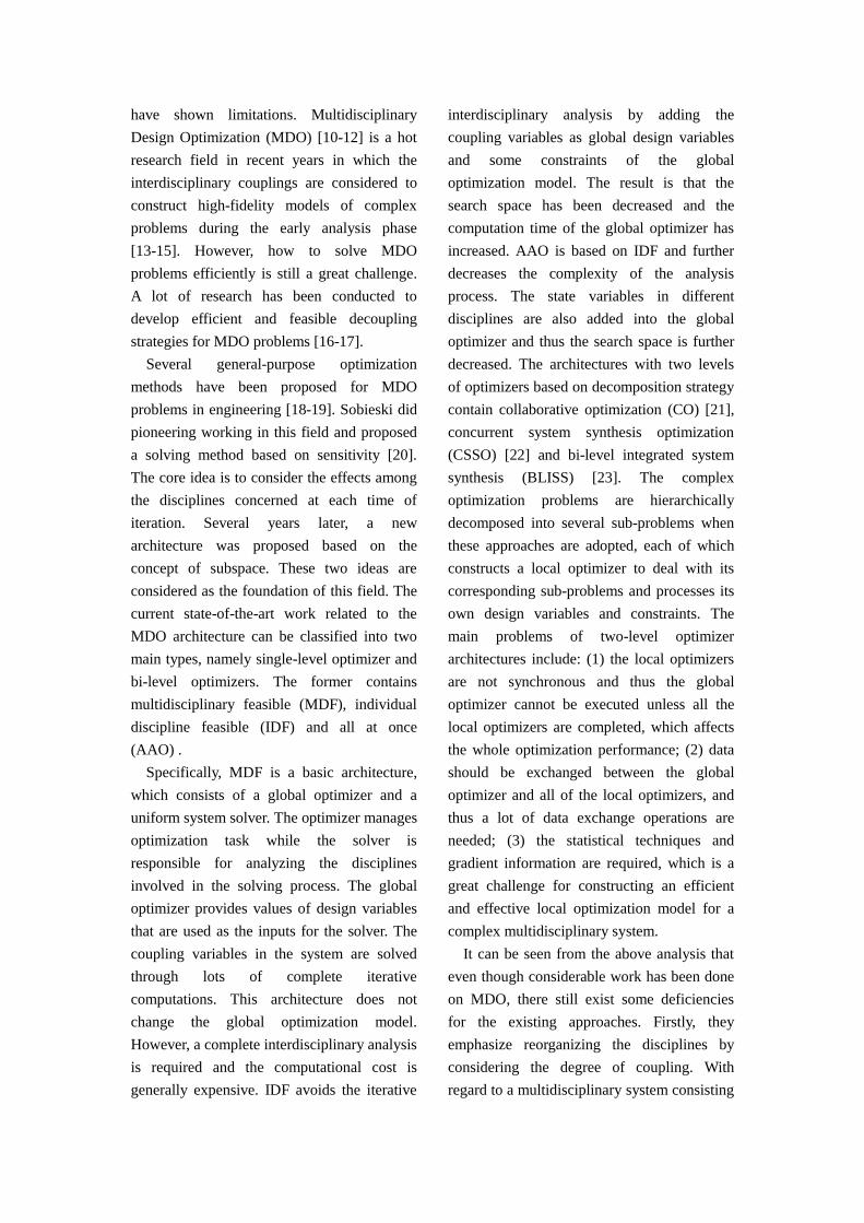
subsystem. The SPD flowchart for solving
MDO problems is given in Fig. 1, which starts
with system initialization by setting the global
design variables, the local design variables for
each discipline and the interdisciplinary
coupling variables. For the sake of clarity, a
number of terms are used in this study: the
coupling variable decoupled among the
subsystems is called the global decoupling
coupling variable (GDCV); the coupling
variable decoupled in one subsystem is called
the local decoupling coupling variable
(LDCV); and the coupling variable without
being decoupled at time of each iteration is
called the reserved coupling variable (RCV).
After the system is initialized, four main
steps need to be taken in the method:
a) Disciplinary analysis: conducting the
disciplinary analysis for each discipline
and updating the output variables;
b) Clustering analysis: executing the
multidisciplinary clustering analysis as
follows:
b.1) Calculating the sensitivity values
between each discipline and each global
optimization objective;
b.2) Conducting the clustering analysis
based on the sensitivity value and then
some subsystems are obtained. At the
same time, adding the corresponding
constraints of GDCVs to the global
optimizer to attain coupling consistency
among subsystems.
c) Subsystem optimization: optimizing all
the subsystems as follows.
c.1) executing the serialization operation in
each subsystem;
c.2) analyzing the subsystem and solving
each output variable in the subsystem in
a sequence according to the directed
graph structure;
c.3) conducting the local optimization
operation for the whole LDCVs in each
subsystem.
d) Global optimization: optimizing the
whole system globally and generating the
new design variable values;
Step b is repeated until the optimization
process converges or the largest number of
iteration has been reached.
Decoupling and optimization in subsystem
System analysis
Initialize system
End
Discipline 1
analysis
Discipline 2
analysis
Discipline k
analysis
Update coupling
variables
Update design
variables
Solver 1 Solver 2 Solver k
Subsystem 1
serialization
Subsystem 2
serialization
Subsystem k
serialization
No
Yes
Global optimizer
Clustering analysis
Sensitivity
calculation
Clustering based on
sensitivity
Local optimizer
1Local optimizer kLocal optimizer 2
Convergence?
Fig. 1 Flowchart of SPD
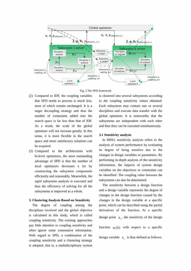
2.2 SPD framework
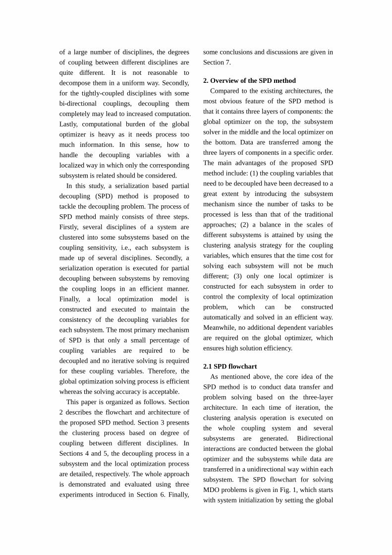
The framework of SPD is shown in Fig. 2.
It can be seen that there are three layers in the
SPD framework. Specifically, the top level is
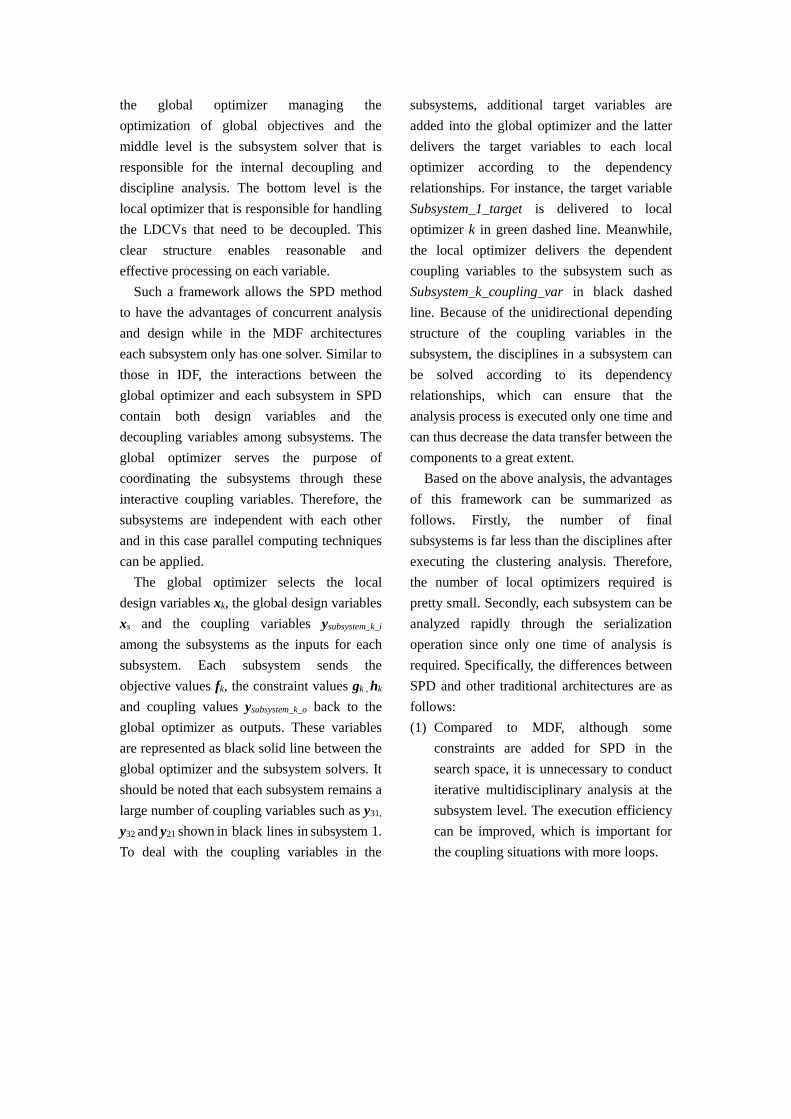
the global optimizer managing the
optimization of global objectives and the
middle level is the subsystem solver that is
responsible for the internal decoupling and
discipline analysis. The bottom level is the
local optimizer that is responsible for handling
the LDCVs that need to be decoupled. This
clear structure enables reasonable and
effective processing on each variable.
Such a framework allows the SPD method
to have the advantages of concurrent analysis
and design while in the MDF architectures
each subsystem only has one solver. Similar to
those in IDF, the interactions between the
global optimizer and each subsystem in SPD
contain both design variables and the
decoupling variables among subsystems. The
global optimizer serves the purpose of
coordinating the subsystems through these
interactive coupling variables. Therefore, the
subsystems are independent with each other
and in this case parallel computing techniques
can be applied.
The global optimizer selects the local
design variables xk, the global design variables
xs and the coupling variables ysubsystem_k_i
among the subsystems as the inputs for each
subsystem. Each subsystem sends the
objective values fk, the constraint values gk , hk
and coupling values ysubsystem_k_o back to the
global optimizer as outputs. These variables
are represented as black solid line between the
global optimizer and the subsystem solvers. It
should be noted that each subsystem remains a
large number of coupling variables such as y31,
y32 and y21 shown in black lines in subsystem 1.
To deal with the coupling variables in the
subsystems, additional target variables are
added into the global optimizer and the latter
delivers the target variables to each local
optimizer according to the dependency
relationships. For instance, the target variable
Subsystem_1_target is delivered to local
optimizer k in green dashed line. Meanwhile,
the local optimizer delivers the dependent
coupling variables to the subsystem such as
Subsystem_k_coupling_var in black dashed
line. Because of the unidirectional depending
structure of the coupling variables in the
subsystem, the disciplines in a subsystem can
be solved according to its dependency
relationships, which can ensure that the
analysis process is executed only one time and
can thus decrease the data transfer between the
components to a great extent.
Based on the above analysis, the advantages
of this framework can be summarized as
follows. Firstly, the number of final
subsystems is far less than the disciplines after
executing the clustering analysis. Therefore,
the number of local optimizers required is
pretty small. Secondly, each subsystem can be
analyzed rapidly through the serialization
operation since only one time of analysis is
required. Specifically, the differences between
SPD and other traditional architectures are as
follows:
(1) Compared to MDF, although some
constraints are added for SPD in the
search space, it is unnecessary to conduct
iterative multidisciplinary analysis at the
subsystem level. The execution efficiency
can be improved, which is important for
the coupling situations with more loops.
Global optimizer
Subsystem 1 solver Subsystem k solverDiscipline 1
analyser
Discipline 2
analyser
Discipline 3
analyser
Discipline
k1 analyser
Discipline
k3 analyser
Discipline
k2 analyser
x1 xs ysubsystem_1_ixk xs ysubsystem_k_i
f1 g1 h1 ysubsystem_1_o fk gk hk ysubsystem_k_o
y31
y32
y21
yk3_k1
yk3_k2
Local
optimizer 1Local
optimizer k
Subsystem_
1_target
Subsystem_
k_target
Subsystem_1_
coupling_varSubsystem_k_
coupling_var
Subsystem_1_c
oupling_varSubsystem_k_
coupling_var
Fig. 2 The SPD framework
(2) Compared to IDF, the coupling variables
that SPD needs to process is much less,
most of which remain unchanged. It is a
target decoupling strategy and thus the
number of constraints added into the
search space is far less than that of IDF.
As a result, the scale of the global
optimizer will not increase greatly. In this
sense, it is more flexible in the search
space and more satisfactory solutions can
be acquired.
(3) Compared to the architectures with
bi-level optimizers, the most outstanding
advantage of SPD is that the number of
local optimizers decreases a lot by
constructing the subsystem components
efficiently and reasonably. Meanwhile, the
rapid subsystem analysis is executed and
thus the efficiency of solving for all the
subsystems is improved as a whole.
3. Clustering Analysis Based on Sensitivity
The degree of coupling among the
disciplines involved and the global objective
is calculated in this study, which is called
coupling sensitivity. The existing approaches
pay little attention to coupling sensitivity and
often ignore some connotative information.
With regard to SPD, a combination of the
coupling sensitivity and a clustering strategy
is adopted, that is, a multidisciplinary system
is clustered into several subsystems according
to the coupling sensitivity values obtained.
Each subsystem may contain one or several
disciplines and execute data transfer with the
global optimizer. It is noteworthy that the
subsystems are independent with each other
and thus they can be executed simultaneously.
3.1 Sensitivity analysis
In MDO, sensitivity analysis refers to the
analysis of system performance by evaluating
its degree of being sensitive due to the
changes in design variables or parameters. By
performing in-depth analysis of the sensitivity
information, the impacts of system design
variables on the objectives or constraints can
be identified. The coupling value between the
subsystems can also be determined.
The sensitivity between a design function
and a design variable represents the degree of
changes in the design function caused by the
changes in the design variable at a specific
point, which can be described using the partial
derivatives of the function. At a specific
design point PX , the sensitivity of the design
function (X)i with respect to a specific
design variable jx is thus defined as follows:
(X), 1,2,..., , 1,2,...,
P
iij X X
j
S i m j nx
(1)
In this expression, m and n are the numbers
of design functions and design variables,
respectively. The larger the value of |ijS |, the
more sensitive the design function (X)i
with respect to jx , i.e.,
jx has a larger
impact on (X)i . ijS represents the
monotonicity of function (X)i with respect
to variable jx . If
ijS <0, it means that (X)i
is monotonically decreasing with respect to
jx . Otherwise, it is monotonically increasing.
Therefore, the sensitivity value expresses two
kinds of information: monotonicity and degree
of being sensitive [24].
The sensitivity of design function |ijS | is
employed to define the degree of coupling.
The larger the value of |ijS | is, the stronger the
coupling degree will be.
3.2 Subsystem clustering based on
sensitivity
The idea that a complex engineering system
is divided into several subsystems can be
regarded as an abstract description of the
problem using smaller and more manageable
sub-problems. Each discipline contains local
variables, global variables, output variables
and its dependent input variables from other
disciplines. The input variables from other
disciplines are the interdisciplinary coupling
variables. Two rules are mainly considered
when the clustering analysis is conducted.
Firstly, the subsystem coupling degree should
be as low as possible, i.e. decreasing the
dependencies between subsystems as much as
possible. Also, there are no additional
constraints for the coupling degree inside one
subsystem. Secondly, the coupling degree
between any subsystem and the global
objective should be as low as possible. In this
way, it can be ensured that the impacts of each
subsystem with regard to the global objective
are uniform and balanced. The traditional
clustering problems usually involve several
features, i.e. the dimension of each point and
its values are represented on the absolute
coordinate system. However, the distances
between a point and the other points are
known for the clustering problems based on
sensitivities among the disciplines, which can
be considered as a representation based on the
relative coordinate system. Based on the
above analysis, the initial centroid must
belong to the current point set. In this study,
an adapted K-means clustering algorithm is
proposed to minimize the sum of the distances
in each cluster. Obviously, different subsystem
partitions lead to different decoupling
variables, and thus have large impacts on the
final subsystem sensitivities. To maximize the
sensitivities among all the subsystems, it is
represented as follows:
1 1 1
M N Pi
jk
i j k
S
EM
(2)
Specifically, E represents the average
subsystem sensitivities; M and N are the
numbers of subsystems and disciplines
respectively; P is the number of disciplines in
each subsystem. It can be seen that the
representation is simple and can precisely
reflect the distance between the subsystems
compared to the standard distance measure
used in the traditional K-means method. The
adopted clustering strategy in this study is
K-means algorithm combined with the global
objective. Suppose that the allowed times of
iteration is T, then the clustering process is as
follows:
a) Calculate the sum of global objective
sensitivities with respect to all the coupling
variables at the k-th time of iteration and
mark it as S. The global objective
sensitivity with respect to each subsystem
is then S/M, represented as AvgS. Construct
a container with M elements, in which each
element records the global objective
sensitivity (with an initial value of 0) with
respect to each subsystem. Select M points
whose sensitivities with respect to other
points are not the largest as the initial
centroids to ensure that the final result is
not the worst;
b) For each left point xi in the point set,
calculate its sensitivity with respect to all
of the subsystems and select the subsystem
with the biggest value. At the same time,
calculate the corresponding global
objective sensitivity value in the container.
If it is bigger than AvgS, abandon the
current selection and consider the
subsystem with the second best sensitivity;
c) Calculate the current subsystem sensitivity
value and re-allocate new centroids;
d) Repeat Steps b and c until k reaches the
maximal number of allowed iteration T, or
the condition (k) (k 1)|| ||E E is
satisfied.
The selection of initial centroids has a large
impact on the final clustering result in
clustering algorithms. In this study, the
selection strategy can to some extent ensure
that good quality can be achieved for the final
result. The reason for this is that for the
problems in this study the number of
disciplines is not too large and thus the
number of clustering points is not large.
4. Decoupling of a Subsystem
After the clustering operation is conducted,
each subsystem is highly correlated as several
coupling loops exist. To improve the
subsystem solving efficiency, SPD is executed
to remove the internal coupling using the
strategy of loop removal in a directed graph
and serialize the disciplines in a subsystem.
After that, the solver for the subsystem can
execute the analysis process in an efficient
way without the need of conducting iteration.
4.1 Connection path between disciplines
A subsystem is composed of one or more
disciplines after the clustering analysis, in
which the disciplines are highly correlated and
dependent on each other. There may be several
coupling variables with a large coupling
degree in each subsystem. Moreover, it is also
possible that there is a number of coupling
loops in a subsystem. It is time-consuming to
perform analysis for each subsystem during an
optimization process. In this study, not all of
the couplings between the disciplines are
considered to be decoupled. Only a part of
them with lower coupling values are
considered to serialize all the disciplines in the
same subsystem to solve the subsystem in a
serializable way without the need of
conducting iteration. Based on the above
analysis, a loop removal method in directed
graphs is adapted in this study with its details
explained in the next paragraph.
Each discipline is regarded as a vertex in
the directed graph based representation of a
subsystem. The coupling variable between two
disciplines means there exists one dependency
and can be regarded as one directed edge. As
shown in Fig. 3, two edges exist between
discipline 1 and discipline 4, which means
there are bidirectional couplings between
these two disciplines. The output variables of
discipline 4 are required when discipline 1 is
analyzed and vice versa. If there is a directed
path between A and B in a directed graph,
there exists a connection path between A and
B. The number of this kind of directed paths is
called the degree of a connection path. As
shown in Fig. 3, no connection path exists
from discipline 4 to discipline 3 whereas there
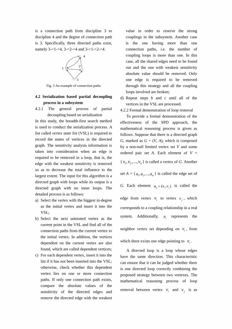
is a connection path from discipline 3 to
discipline 4 and the degree of connection path
is 3. Specifically, three directed paths exist,
namely 3->1->4, 3->2->4 and 3->1->2->4.
12
4
3
Fig. 3 An example of connection paths
4.2 Serialization based partial decoupling
process in a subsystem
4.2.1 The general process of partial
decoupling based on serialization
In this study, the breadth-first search method
is used to conduct the serialization process. A
list called vertex state list (VSL) is required to
record the states of vertices in the directed
graph. The sensitivity analysis information is
taken into consideration when an edge is
required to be removed in a loop, that is, the
edge with the weakest sensitivity is removed
so as to decrease the total influence to the
largest extent. The input for this algorithm is a
directed graph with loops while its output is a
directed graph with no inner loops. The
detailed process is as follows:
a) Select the vertex with the biggest in-degree
as the initial vertex and insert it into the
VSL;
b) Select the next untreated vertex as the
current point in the VSL and find all of the
connection paths from the current vertex to
the initial vertex. In addition, the vertices
dependent on the current vertex are also
found, which are called dependent vertices;
c) For each dependent vertex, insert it into the
list if it has not been inserted into the VSL;
otherwise, check whether this dependent
vertex lies on one or more connection
paths. If only one connection path exists,
compare the absolute values of the
sensitivity of the directed edges and
remove the directed edge with the weakest
value in order to reserve the strong
couplings in the subsystem. Another case
is the one having more than one
connection paths, i.e. the number of
coupling loops is more than one. In this
case, all the shared edges need to be found
out and the one with weakest sensitivity
absolute value should be removed. Only
one edge is required to be removed
through this strategy and all the coupling
loops involved are broken;
d) Repeat steps b and c until all of the
vertices in the VSL are processed.
4.2.2 Formal demonstration of loop removal
To provide a formal demonstration of the
effectiveness of the SPD approach, the
mathematical reasoning process is given as
follows. Suppose that there is a directed graph
G, marked as G = (V, A), which is composed
by a non-null limited vertex set V and some
ordered pair set A. Each element of V =
{ 1 2, ,..., nv v v } is called a vertex of G. Another
set A = {1 2, ,..., ma a a } is called the edge set of
G. Each element ( , )ij i ja v v is called the
edge from vertex iv to vertex jv , which
corresponds to a coupling relationship in a real
system. Additionally, iN represents the
neighbor vertex set depending on iv , from
which there exists one edge pointing to iv .
A directed loop is a loop whose edges
have the same direction. This characteristic
can ensure that it can be judged whether there
is one directed loop correctly combining the
proposed strategy between two vertexes. The
mathematical reasoning process of loop
removal between vertex iv and jv is as
follows:
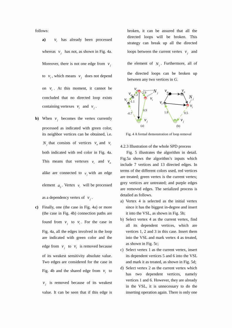
a) iv has already been processed
whereas jv has not, as shown in Fig. 4a.
Moreover, there is not one edge from jv
to iv , which means jv does not depend
on iv . At this moment, it cannot be
concluded that no directed loop exists
containing vertexes iv and jv .
b) When jv becomes the vertex currently
processed as indicated with green color,
its neighbor vertices can be obtained, i.e.
jN that consists of vertices nv and iv
both indicated with red color in Fig. 4a.
This means that vertexes iv and nv
alike are connected to jv with an edge
element ija . Vertex
iv will be processed
as a dependency vertex of jv .
c) Finally, one (the case in Fig. 4a) or more
(the case in Fig. 4b) connection paths are
found from jv to iv . For the case in
Fig. 4a, all the edges involved in the loop
are indicated with green color and the
edge from jv to lv is removed because
of its weakest sensitivity absolute value.
Two edges are considered for the case in
Fig. 4b and the shared edge from iv to
jv is removed because of its weakest
value. It can be seen that if this edge is
broken, it can be assured that all the
directed loops will be broken. This
strategy can break up all the directed
loops between the current vertex jv and
the element of jN . Furthermore, all of
the directed loops can be broken up
between any two vertices in G.
-0.7 1.8 0.5
-1.1
0.9
(a) (b)
iv
jv
mvnv
lvlv
iv
jv
mv nv1.2
2.9
jNjN
Fig. 4 A formal demonstration of loop removal
4.2.3 Illustration of the whole SPD process
Fig. 5 illustrates the algorithm in detail.
Fig.5a shows the algorithm’s inputs which
include 7 vertices and 13 directed edges. In
terms of the different colors used, red vertices
are treated; green vertex is the current vertex;
grey vertices are untreated; and purple edges
are removed edges. The serialized process is
detailed as follows.
a) Vertex 4 is selected as the initial vertex
since it has the biggest in-degree and insert
it into the VSL, as shown in Fig. 5b;
b) Select vertex 4 as the current vertex, find
all its dependent vertices, which are
vertices 1, 2 and 3 in this case. Insert them
into the VSL and mark vertex 4 as treated,
as shown in Fig. 5c;
c) Select vertex 1 as the current vertex, insert
its dependent vertices 5 and 6 into the VSL
and mark it as treated, as shown in Fig. 5d;
d) Select vertex 2 as the current vertex which
has two dependent vertices, namely
vertices 1 and 6. However, they are already
in the VSL, it is unnecessary to do the
inserting operation again. There is only one
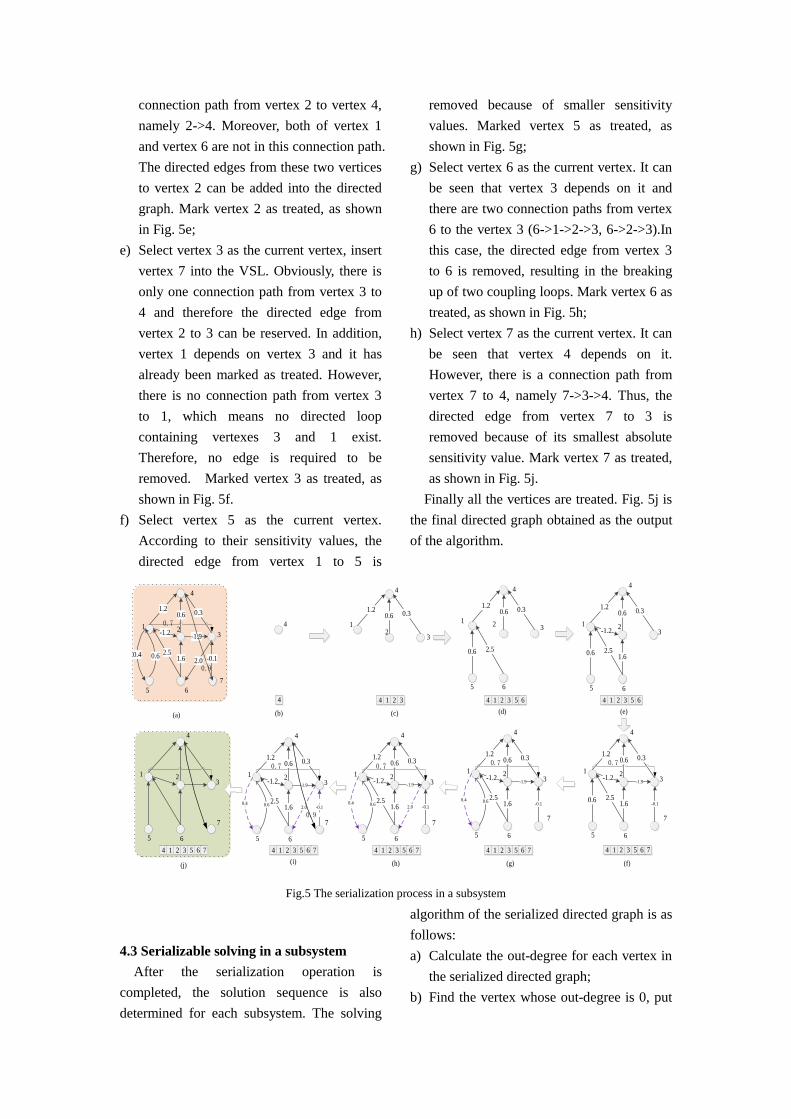
connection path from vertex 2 to vertex 4,
namely 2->4. Moreover, both of vertex 1
and vertex 6 are not in this connection path.
The directed edges from these two vertices
to vertex 2 can be added into the directed
graph. Mark vertex 2 as treated, as shown
in Fig. 5e;
e) Select vertex 3 as the current vertex, insert
vertex 7 into the VSL. Obviously, there is
only one connection path from vertex 3 to
4 and therefore the directed edge from
vertex 2 to 3 can be reserved. In addition,
vertex 1 depends on vertex 3 and it has
already been marked as treated. However,
there is no connection path from vertex 3
to 1, which means no directed loop
containing vertexes 3 and 1 exist.
Therefore, no edge is required to be
removed. Marked vertex 3 as treated, as
shown in Fig. 5f.
f) Select vertex 5 as the current vertex.
According to their sensitivity values, the
directed edge from vertex 1 to 5 is
removed because of smaller sensitivity
values. Marked vertex 5 as treated, as
shown in Fig. 5g;
g) Select vertex 6 as the current vertex. It can
be seen that vertex 3 depends on it and
there are two connection paths from vertex
6 to the vertex 3 (6->1->2->3, 6->2->3).In
this case, the directed edge from vertex 3
to 6 is removed, resulting in the breaking
up of two coupling loops. Mark vertex 6 as
treated, as shown in Fig. 5h;
h) Select vertex 7 as the current vertex. It can
be seen that vertex 4 depends on it.
However, there is a connection path from
vertex 7 to 4, namely 7->3->4. Thus, the
directed edge from vertex 7 to 3 is
removed because of its smallest absolute
sensitivity value. Mark vertex 7 as treated,
as shown in Fig. 5j.
Finally all the vertices are treated. Fig. 5j is
the final directed graph obtained as the output
of the algorithm.
1.20.6 0.3
0.4 0.6
-1.2-1.9
-0.11.62.5
2.0
1 23
4
5 6
7
1.20.6 0.3
1.20.6 0.3
0.6 2.5
1.20.6 0.3
0.6 2.51.6
-1.2
4
1 23
5 6
1.20.6 0.3
0.6 2.51.6
-1.2
4
1 23
5 6
7
-1.9
-0.1
1.20.6 0.3
2.51.6
-1.2
4
1 23
5 6
7
-1.9
-0.10.4 0.6
1.20.6 0.3
2.51.6
-1.2
4
1 23
5 6
7
-1.9
-0.10.4 0.6
2.0
1.20.6 0.3
2.51.6
-1.2
4
1 23
5 6
-1.9
-0.10.4 0.6
2.0
4
1 23
5 6
4
12
3
4
4
1 23
5 6
4 4 1 2 3 4 1 2 3 5 6 4 1 2 3 5 6
4 1 2 3 5 6 74 1 2 3 5 6 74 1 2 3 5 6 74 1 2 3 5 6 74 1 2 3 5 6 7
7 7
(a) (b) (c) (d) (e)
(f)(g)(i)(j) (h)
0.7
0.9
0.70.7
0.9
0.70.7
Fig.5 The serialization process in a subsystem
4.3 Serializable solving in a subsystem
After the serialization operation is
completed, the solution sequence is also
determined for each subsystem. The solving
algorithm of the serialized directed graph is as
follows:
a) Calculate the out-degree for each vertex in
the serialized directed graph;
b) Find the vertex whose out-degree is 0, put

it into the sequence solving list and
decrease all of the out-degree of its
dependent vertices by one;
c) Repeat Step (b) until all the vertices have
been placed in the solving sequence list.
Take Fig. 4j as an example, the calculation
process is detailed as follows:
a) The out-degree of vertex 7 is 0, put it in
the solving sequence list and decrease the
out-degree of vertex 4 by one.
b) The out-degree of the initial vertex 4 is 0,
put it in the solving sequence list and
decrease the out-degree of vertices 1, 2 and
3 by one;
c) The out-degree of vertex 3 is 0 and put it in
the solving sequence list. Decrease the
out-degree of vertices 1 and 2 by one;
d) The out-degrees of vertex 2 is 0, thus it is
put in the solving sequence list. Decrease
the out-degree of vertices 1 and 6 by one;
e) The out-degrees of vertex 1 is 0 and thus
they are put in the solving sequence list.
Decrease the out-degree of vertices 5 and 6
by one;
Put vertices 5 and 6 in the solving sequence
list. The final solving sequence list is then
obtained as (7-4-3-2-1-6-5). The subsystem
solver is executed according to this sequence
without the need to perform iteration
Note that many coupling variables among
different disciplines can be reserved by using
the serialized decoupling strategy. As shown
in this example with initial 13 coupling
variables, 10 coupling variables are reserved
after the subsystem decoupling operation has
been executed. The subsequent local optimizer
only needs to deal with three decoupled
variables. Compared to IDF’s operation of
adding 13 constraints to be considered by the
global optimizer, the proposed SPD is much
more efficient in terms of search space
exploration. Moreover, each subsystem solver
only run one time whereas in MDF three
iteration-based analysis will be required. This
shows that solving efficiency is significantly
improved. In particular, for the system with
more complicated coupled relationships, the
performance improvement achieved by SPD is
much more prominent.
5. Local optimization in a subsystem
As mentioned above, most of the coupling
variables can be analyzed serially after the
previous step is executed. A small part of
variables need to be decoupled. These
variables can be regarded as design variables
and some corresponding constraints are
appended in the global optimization model.
However, it will possibly make the global
optimization model to be excessively
constrained and as a result the search space is
greatly narrowed down.
In this study, a local optimization method
is proposed to handle the coupling variables
within a subsystem and keep the whole system
consistent. In this case, the key issue is how to
ensure the efficiency of solving the global
optimization model and the acceptance of
local dynamical optimization models.
Meanwhile, it is also important to deal with
the related decoupled variables in a reasonable
way. Based on the above analysis, the
construction of a proper local optimization
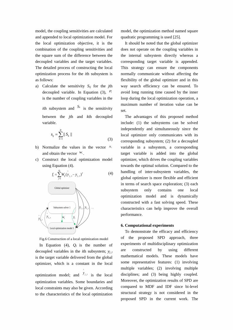
model is necessitated. As shown in Fig. 6, for
each time of iteration, the bottom local
optimizer accepts the target variables from the
global optimizer and the output variables of its
corresponding subsystem. The decoupled
variables in each subsystem are regarded as
the optimization variables of a local
optimization model. Each local optimizer is
only conducted for its corresponding
subsystem to solve the decoupled variables.
Moreover, the coupling sensitivities of the
decoupled variables for its corresponding
subsystem are also taken into account since
different decoupled variables make distinct
impacts on the same subsystem. To precisely
reflect the impacts on a local optimization
model, the coupling sensitivities are calculated
and appended to local optimization model. For
the local optimization objective, it is the
combination of the coupling sensitivities and
the square sum of the difference between the
decoupled variables and the target variables.
The detailed process of constructing the local
optimization process for the ith subsystem is
as follows:
a) Calculate the sensitivity Sij for the jth
decoupled variable. In Equation (3), iP
is the number of coupling variables in the
ith subsystem and kS is the sensitivity
between the jth and kth decoupled
variable.
1
|| ||iP
ij k
k
s S
(3)
b) Normalize the values in the vector iS
and obtain the vector iW .
c) Construct the local optimization model
using Equation (4).
^2
__
1
( )iQ
i ij j tj t
j
f W y y
(4)
Local optimization model 1
Global optimizer
2 _ ty 3_ tySubsystem solver 1
1y^
2 _ ty^
3_ ty 1w
Fig.6 Construction of a local optimization model
In Equation (4), Qi is the number of
decoupled variables in the ith subsystem; yj_t
is the target variable delivered from the global
optimizer, which is a constant in the local
optimization model; and
^
_j ty
is the local
optimization variables. Some boundaries and
local constraints may also be given. According
to the characteristics of the local optimization
model, the optimization method named square
quadratic programming is used [25].
It should be noted that the global optimizer
does not operate on the coupling variables in
the internal subsystem directly whereas a
corresponding target variable is appended.
This strategy can ensure the components
normally communicate without affecting the
flexibility of the global optimizer and in this
way search efficiency can be ensured. To
avoid long running time caused by the inner
loop during the local optimization operation, a
maximum number of iteration value can be
set.
The advantages of this proposed method
include: (1) the subsystems can be solved
independently and simultaneously since the
local optimizer only communicates with its
corresponding subsystem; (2) for a decoupled
variable in a subsystem, a corresponding
target variable is added into the global
optimizer, which drives the coupling variables
towards the optimal solution. Compared to the
handling of inter-subsystem variables, the
global optimizer is more flexible and efficient
in terms of search space exploration; (3) each
subsystem only contains one local
optimization model and is dynamically
constructed with a fast solving speed. These
characteristics can help improve the overall
performance.
6. Computational experiments
To demonstrate the efficacy and efficiency
of the proposed SPD approach, three
experiments of multidisciplinary optimization
are constructed by using different
mathematical models. These models have
some representative features: (1) involving
multiple variables; (2) involving multiple
disciplines; and (3) being highly coupled.
Moreover, the optimization results of SPD are
compared to MDF and IDF since bi-level
structural strategy is not considered in the
proposed SPD in the current work. The
experiments are conducted on the
OpenMDAO [26] platform developed by
NASA.
6.1 Partial decoupling of a single subsystem
The first typical test application is called the
Sellar [27] problem which has a mathematical
model as follows:
Minimize:
22
1 2 1
yf x z y e
(5)
Design variables: 1x ,
1z ,2z
Subject to: 2
1 1 1 2 20.2y z x z y
2 1 1 2y y z z
In this example, two disciplines are entirely
coupled through 1y and 2y even it looks
simple. It is solved through three architectures,
namely SPD, MDF and IDF. This problem is
directly described as one subsystem, and thus
clustering analysis is not required. In the SPD
method, 1y is decoupled and a local optimizer
is constructed to deal with it. This experiment
is used to demonstrate the effectiveness of
partial decoupling and local optimization.
Table 1 shows the result of Experiment 1. It
can be seen that IDF has the optimal result but
requires the longest time. On the contrary,
MDF’s execution efficiency is better than the
others but it has the worst results. The
proposed SPD method lies between the two in
terms of both efficiency and performance.
Moreover, the final two coupling variables
converge to the same position. The
experimental results indicate that the proposed
SPD method has good effectiveness in terms
of the partial decoupling strategy.
Table 1. Results of Experiment 1
SPD IDF MDF
Optimal positions:
1z 1.977670 1.977658 1.977639
2z 0.0 0.0 0.0
1x 0.0 0.0 0.0
Coupling variables:
1y
3.16 3.16 3.16
2y 3.755309 3.755383 3.755278
Optimal f 3.1833932 3.1833914 3.1833937
Runtime(s) 0.555 0.641 0.251
6.2 Serializable decoupling of
multidisciplinary problems
To demonstrate the clustering analysis and
serializable decoupling strategy, a large-scale
complicated system is constructed with the
help of CASCADE [28] and is shown below:
Minimize:
22 2
1 2 1 41 8 3 4 60.5 0.8 2.5y
f x z y e x x y y y
(6)
Design variables:1x ,
3x ,41x ,
42x ,5x ,
8x ,1z ,
2z
Subject to: 2
1 1 1 2 20.2y z x z y
2 1 1 2y y z z
3
3 1 2 3 1 50.5 2y z z x y y
2
4 2 41 42 1 30.5y z x x y y
5 1 2 5 2 3 72.5y z z x y y y
2
6 1 4 8y z y y
7 1 2 1 6 90.2 3y z z y y y
8 1 2 8 2 51.5y z z x y y
9 1 4y z y
1
2
3
4
5
6
7
8
9
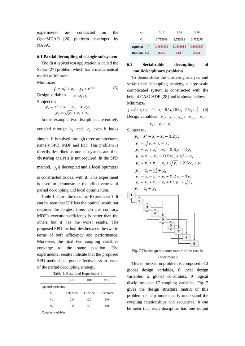
Fig. 7 The design structure matrix of the case in
Experiment 2
This optimization problem is composed of 2
global design variables, 8 local design
variables, 2 global constraints, 9 logical
disciplines and 17 coupling variables. Fig. 7
gives the design structure matrix of this
problem to help more clearly understand the
coupling relationships and sequences. It can
be seen that each discipline has one output
variable in this case.
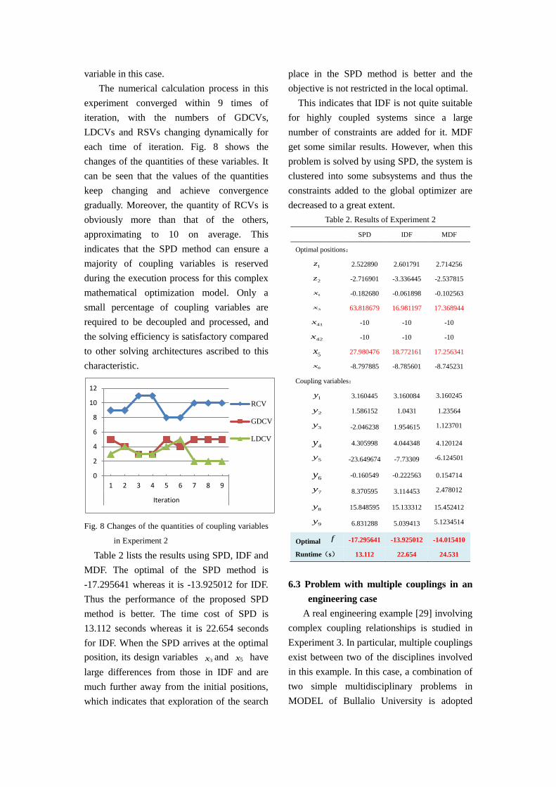
The numerical calculation process in this
experiment converged within 9 times of
iteration, with the numbers of GDCVs,
LDCVs and RSVs changing dynamically for
each time of iteration. Fig. 8 shows the
changes of the quantities of these variables. It
can be seen that the values of the quantities
keep changing and achieve convergence
gradually. Moreover, the quantity of RCVs is
obviously more than that of the others,
approximating to 10 on average. This
indicates that the SPD method can ensure a
majority of coupling variables is reserved
during the execution process for this complex
mathematical optimization model. Only a
small percentage of coupling variables are
required to be decoupled and processed, and
the solving efficiency is satisfactory compared
to other solving architectures ascribed to this
characteristic.
Fig. 8 Changes of the quantities of coupling variables
in Experiment 2
Table 2 lists the results using SPD, IDF and
MDF. The optimal of the SPD method is
-17.295641 whereas it is -13.925012 for IDF.
Thus the performance of the proposed SPD
method is better. The time cost of SPD is
13.112 seconds whereas it is 22.654 seconds
for IDF. When the SPD arrives at the optimal
position, its design variables 3x and 5x have
large differences from those in IDF and are
much further away from the initial positions,
which indicates that exploration of the search
place in the SPD method is better and the
objective is not restricted in the local optimal.
This indicates that IDF is not quite suitable
for highly coupled systems since a large
number of constraints are added for it. MDF
get some similar results. However, when this
problem is solved by using SPD, the system is
clustered into some subsystems and thus the
constraints added to the global optimizer are
decreased to a great extent.
Table 2. Results of Experiment 2
SPD IDF MDF
Optimal positions:
1z 2.522890 2.601791 2.714256
2z -2.716901 -3.336445 -2.537815
1x
-0.182680 -0.061898 -0.102563
3x
63.818679 16.981197 17.368944
41x -10 -10 -10
42x -10 -10 -10
5x 27.980476 18.772161 17.256341
8x
-8.797885 -8.785601 -8.745231
Coupling variables:
1y 3.160445 3.160084 3.160245
2y 1.586152 1.0431 1.23564
3y -2.046238 1.954615 1.123701
4y 4.305998 4.044348 4.120124
5y -23.649674 -7.73309 -6.124501
6y -0.160549 -0.222563 0.154714
7y 8.370595 3.114453 2.478012
8y 15.848595 15.133312 15.452412
9y 6.831288 5.039413 5.1234514
Optimal f -17.295641 -13.925012 -14.015410
Runtime(s) 13.112 22.654 24.531
6.3 Problem with multiple couplings in an
engineering case
A real engineering example [29] involving
complex coupling relationships is studied in
Experiment 3. In particular, multiple couplings
exist between two of the disciplines involved
in this example. In this case, a combination of
two simple multidisciplinary problems in
MODEL of Bullalio University is adopted
0
2
4
6
8
10
12
1 2 3 4 5 6 7 8 9
Iteration
RCV
GDCV
LDCV
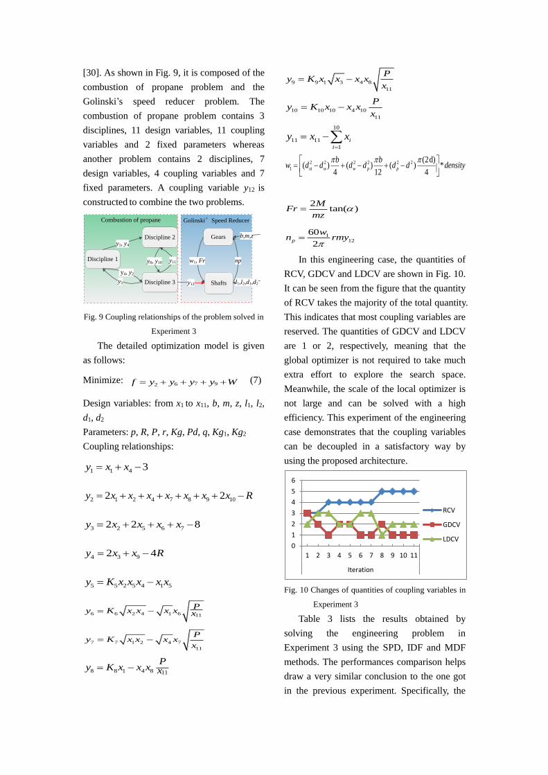
[30]. As shown in Fig. 9, it is composed of the
combustion of propane problem and the
Golinski’s speed reducer problem. The
combustion of propane problem contains 3
disciplines, 11 design variables, 11 coupling
variables and 2 fixed parameters whereas
another problem contains 2 disciplines, 7
design variables, 4 coupling variables and 7
fixed parameters. A coupling variable y12 is
constructed to combine the two problems.
Golinski’Speed ReducerCombustion of propane
Discipline 2
Discipline 1
Discipline 3
Gears
Shafts
y1, y4
y4, y2
y5
y8, y10 y11 w1, Fr np
y12
b,m,z
l1,l2,d1,d2
Fig. 9 Coupling relationships of the problem solved in
Experiment 3
The detailed optimization model is given
as follows:
Minimize: 7 962f y y y y W (7)
Design variables: from x1 to x11, b, m, z, l1, l2,
d1, d2
Parameters: p, R, P, r, Kg, Pd, q, Kg1, Kg2
Coupling relationships:
1 1 4 3y x x
2 1 2 4 7 8 9 102 2y x x x x x x x R
3 2 5 6 72 2 8y x x x x
4 3 92 4y x x R
5 5 2 5 4 1 5y K x x x x x
6 6 2 4 1 6 11
Py K x x x x x
7 7 1 2 4 7
11
Py K x x x x
x
8 8 1 4 8 11
Py K x x x x
9 9 1 3 4 8
11
Py K x x x x
x
10 10 10 4 10
11
Py K x x x
x
10
11 11
1
i
i
y x x
2 2 2 2 2 2
1
(2d)( ) ( ) ( ) *
4 12 4st w w p p
b bw d d d d d d density
2tan( )
MFr
mz
112
60
2p
wn rmy
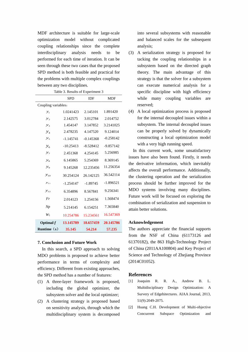
In this engineering case, the quantities of
RCV, GDCV and LDCV are shown in Fig. 10.
It can be seen from the figure that the quantity
of RCV takes the majority of the total quantity.
This indicates that most coupling variables are
reserved. The quantities of GDCV and LDCV
are 1 or 2, respectively, meaning that the
global optimizer is not required to take much
extra effort to explore the search space.
Meanwhile, the scale of the local optimizer is
not large and can be solved with a high
efficiency. This experiment of the engineering
case demonstrates that the coupling variables
can be decoupled in a satisfactory way by
using the proposed architecture.
Fig. 10 Changes of quantities of coupling variables in
Experiment 3
Table 3 lists the results obtained by
solving the engineering problem in
Experiment 3 using the SPD, IDF and MDF
methods. The performances comparison helps
draw a very similar conclusion to the one got
in the previous experiment. Specifically, the
0
1
2
3
4
5
6
1 2 3 4 5 6 7 8 9 10 11
Iteration
RCV
GDCV
LDCV
MDF architecture is suitable for large-scale
optimization model without complicated
coupling relationships since the complete
interdisciplinary analysis needs to be
performed for each time of iteration. It can be
seen through these two cases that the proposed
SPD method is both feasible and practical for
the problems with multiple complex couplings
between any two disciplines.
Table 3. Results of Experiment 3
SPD IDF MDF
Coupling variables:
1y 1.0241423 2.145101 1.891420
2y 2.142575 3.012784 2.014752
3y 1.454147 3.147852 3.2141025
4y 2.478235 4.147520 9.124014
5y -1.145741 -0.145368 -0.258142
6y -10.25413 -8.528412 -9.857142
7y 2.451368 4.254145 5.256985
8y 6.145865 5.254369 8.369145
9y 9.145268 12.235456 11.256354
10y 30.254124 26.142125 36.542114
11y
-1.254147 -1.89745 -1.896521
12y 6.354896 8.567841 9.256341
Fr 2.014123 1.254156 1.568474
Np 5.214145 6.154251 7.365840
W1 10.254786 15.234561 16.547369
Optimal f
13.145789 18.657459 20.145786
Runtime(s) 35.145 54.214 57.235
7. Conclusion and Future Work
In this search, a SPD approach to solving
MDO problems is proposed to achieve better
performance in terms of complexity and
efficiency. Different from existing approaches,
the SPD method has a number of features:
(1) A three-layer framework is proposed,
including the global optimizer, the
subsystem solver and the local optimizer;
(2) A clustering strategy is proposed based
on sensitivity analysis, through which the
multidisciplinary system is decomposed
into several subsystems with reasonable
and balanced scales for the subsequent
analysis;
(3) A serialization strategy is proposed for
tacking the coupling relationships in a
subsystem based on the directed graph
theory. The main advantage of this
strategy is that the solver for a subsystem
can execute numerical analysis for a
specific discipline with high efficiency
while many coupling variables are
reserved;
(4) A local optimization process is proposed
for the internal decoupled issues within a
subsystem. The internal decoupled issues
can be properly solved by dynamically
constructing a local optimization model
with a very high running speed.
In this current work, some unsatisfactory
issues have also been found. Firstly, it needs
the derivative information, which inevitably
affects the overall performance. Additionally,
the clustering operation and the serialization
process should be further improved for the
MDO systems involving many disciplines.
Future work will be focused on exploring the
combination of serialization and suspension to
attain better solutions.
Acknowledgement
The authors appreciate the financial supports
from the NSF of China (61173126 and
61370182), the 863 High-Technology Project
of China (2011AA100804) and Key Project of
Science and Technology of Zhejiang Province
(2014C01052).
References
[1] Joaquim R. R. A., Andrew B. L.
Multidisciplinary Design Optimization: A
Survery of Edgehitectures. AIAA Journal, 2013,
51(9):2049-2075.
[2] Huang C.H. Development of Multi-objective
Concurrent Subspace Optimization and
Visualization Methods for Multidisciplinary
Design (Ph.D thesis). Department of Mechanical
and Aerospace Engineering, State University of
New York at Buffalio, April 2003.
[3] Mastroddi F., Gemma S. Analysis of Pareto
Frontiers for Multidisciplinary Design
Optimization of Aircraft. Aerospace Science and
Technology, 2013, 28(1):40-55.
[4] Chebbah M. S., Naceur H., Hecini M. Rapid
Coupling Optimization Method for a Tube
Hydroforming Process. Proceedings of the
Institution of Mechanical Engineers, Part B:
Journal of Engineering Manufacture,
2010,224(2):245-256.
[5] Lin L., Liu M. Z., Tang J., Zhao Z. B., Ge M.
G. The Coupling Relationship among
Bottleneck Shifting Factors in Job Shop.
Proceedings of the Institution of Mechanical
Engineers, Part B: Journal of Engineering
Manufacture, 2013, 227(9): 1373-1381.
[6] Zhang P., Chen X. A. Thermal-mechanical
Coupling Model-based Dynamical Properties
Analysis of a Motorized Spindle System.
Proceedings of the Institution of Mechanical
Engineers, Part B: Journal of Engineering
Manufacture, 2014, 1-12.
[7] Sobieszezanski-Sobieski J.Leonard L., Sirkett D.
M. Engineering a New Wrist Joint Replacement
Prosthesis-a Multidisciplinary Approach.
Journal of Engineering Manufacture, 2002,
216:1297-1302.
[8] Weck O. D., Agte J., Sobieszezanski-Sobieski J.
State-of- the-art and Future trends in
Multidisciplinary Design Optimization. In:
Proceedings of the 48th
AIAA/ASME/ASCE/AHS/ACS Structures,
Structural Dynamics, and Materials Conference,
AIAA-2007-1905, 2007, April 23-26.
[9] Myers R. H., Montogomery D. C. Response
Surface Methodology: Process and Product
Optimization using Designed Experiments. New
York: Wiley, 1995.
[10] Braun R. D., Kroo I. M. Development and
Application of the Collaborative Optimization
Architecture in a Multidisciplinary Design
Environment. In Proceedings of the
ICASE/NASA Langey Workshop on
Multidisciplinary Design Optimization,
Hampton, Virginia, 1995, 98-116.
[11] Zadeh P. M., Toropov V. V., Wood A. S.
Metamodel-based Collaborative Optimization
Framework. Structural and Multidisciplinary
Optimization, 2009, 38(2):103-115.
[12] Sobieszezanski-Sobieski J, Chopra I.
Multidisciplinary Optimization of Aeronautical
System. Journal of Aircraft, 1990, 12: 977-978.
[13] Li Y., Lu Z., Michalek J. J. Diagonal Quadratic
Approximation for Parallelization of Analytical
Target Cascading. Journal of Mechanical Design,
2008, 130(5):051402-1-051402-11.
[14] Tappeta R. V., Renaud J. E. Multi-objective
Collaborative Optimization. Journal of
Mechanical Design, 1997, 119(3):403-411.
[15] Simpson T. W., Mistree F., Korte J. J. Kriging
Models for Global Approximation in
Simulation-based Multidisciplinary Design
Optimization. AIAA Journal, 2001,
39(12):2233-2241.
[16] Han M. H.. Multidisciplinary Design
Optimization Approaches and Technique
Research for Complex Engineering Systems.
Beijing University of Aeronautics and
Astronautics.
[17] Yao W., Chen X. Q., Luo W. C. Review of
Uncertainty-based Multidisciplinary Design
Optimization Methods for Aerospace Vehicles.
Progress In Aerospace Sciences, 2011,
47(6):450-479.
[18] Wang D. H., Hu F., Ma Z. Y. A CAD/CAE
Integrated Framework for Structural Design
Optimization Using Sequential Approximation
Optimization. Advances in Engineering
Software, 2014,76:56-68.
[19] Patnaik S.N., Hopkins D.A. General Purpose
Optimization Method for Multidisciplinary
Design Applications. Advances in Engineering
Software, 2000, 31:57-63.
[20] Sobieszezanski-Sobieski J. Sensitivity of
Complex Internally Coupled Systems. AIAA
Journal, 1990,28(1):153-160.
[21] Braun R. D., Kroo I. M. Development and
Application of the Collaborative Optimization
Architecture in a Multidisciplinary Design
Environment. SIAM Journal, 1995, 98-116.
[22] Sell R. S., Batill S. M., Renaud J. E. Response
Surface Based Concurrent Subspace
Optimization for Multidisciplinary System
Design. AIAA, 1996, 96-0714.
[23] Sobieszczanski-Sobieski J., Agte J. S. and
Sandusky R. R. Bi-Level Integrated System
Synthesis (BLISS). NASA /TM-1998-208715.
[24] Qiu Q. Y., Feng P. E., Dong L. G. Approaches
for Analyzing the Optimization Results Based
on the Sensitivity Information. Journal of
Zhejiang university, 2000, 34(6):603-607.
[25] Irene R. L., Ramon H., Charles E. Quadratic
Programming Feature Selection. Journal of
Machine Learning Research, 2010,
11:1491-1516.
[26] Justin G., Kenneth T. M. Standard Platform for
Benchmarking Multidisciplinary Design
Analysis and Optimization Architectures. AIAA
Journal, 2013, 51(10).
[27] Chan L. Evaluation of Two Concurrent Design
Approaches in Multidisciplinary Design
Optimization . NRC report LM-A-077, 2001.
[28] Hulme K. F., Bloebaum C L. Development of
CASCADE- A Multidisciplinary Design Test
Simulator. AIAA, 1996.
[29] Roy R., Hinduja S., Teti R. Recent Advances in
Engineering Design Optimization: Challenges
and Future Trends. CIRP Annals –
Manufacturing Technology, 2008,
57(2):697-715.
[30] Parashar. S. Decision Support Tool for
Multidisciplinary Design Optimization Using
Multi-domain Decomposition. Master of
Science Thesis, 2004,29-34.