a short review on panel data econometrics

A Short Review on Panel Data Econometrics

Patrick GAGLIARDINIUniversita della Svizzera Italiana

May 2013

Patrick Gagliardini (USI) A Short Review on Panel Data Econometrics May 2013 1 / 78

OUTLINE

1. Fixed and random effects in linear panel data models

2. IV estimation of linear dynamic panel data models

3. Nonlinear panel data models


1. FIXED AND RANDOM EFFECTS IN LINEAR PANEL DATA MODELS


1.1 LINEAR PANEL DATA MODELS

Panel data are doubly indexed by individual and time:

yi,t, i = 1, ..., n, t = 1, ..., T

Pooling cross-sectional and time series information allows to

i) avoid bias from unobservable individual heterogeneity

ii) distinguish common parameters from individual specific effects and timespecific effects

iii) study the dynamics at the micro-level

iv) ...

Econometric analysis of panel data started with Mundlak (1961), (1978), Hoch(1962), Balestra, Nerlove (1966)


Two linear specifications that are extreme approaches to addressunobservable individual heterogeneity:

i) Full homogeneity: Pooled regression

yi,t = α + x′i,tβ + εi,t

ii) Full heterogeneity: A system of equations

yi,t = αi + x′i,tβi + εi,t

The linear panel data literature has mostly focused on the intermediatespecification:

yi,t = αi + x′i,tβ + εi,t

where β is a common parameter and the αi are the individual effects


The individual effects vary across individuals but are constant over time; theycapture (parsimoniously) the specificities of individual behaviours

We distinguish two approaches:

i) Fixed effects: The αi, for i = 1, ..., n, are unknown constants (to beincluded among the - nuisance - parameters)

ii) Random effects: The αi, for i = 1, ..., n, are unobservable randomvariables (to be incorporated in the error terms)

Fixed and random effects yield different model interpretations and differentestimators


1.2 FIXED EFFECTS

i) The model:yi,t = αi + x′i,t

1×K

β + εi,t

where:

A.1: The errors εi,t are i.i.d. across individuals and time dates, with E[εi,t] = 0and V[εi,t] = σ2, for all i and t

A.2: The regressor xi,t is independent of the error term εj,s, for all i, j and t, s

Compact form:yi

T×1= STαi + Xi

T×Kβ + εi

where yi = (yi,1, ..., yi,T)′ and ST = (1, ..., 1)′ is a T-dimensional vector of ones,and

ynT×1

= (In ⊗ ST)︸︷︷︸≡D

α + XnT×K

β + ε ≡ Wγ + ε (1)

where y = (y′1, ..., y′n)′, α = (α1, ..., αn)′, γ = (α′, β′)′ and W = [D X]


Equation (1) written explicitly:⎛⎜⎜⎜⎜⎜⎜⎜⎜⎜⎜⎜⎜⎜⎜⎜⎜⎜⎜⎜⎜⎜⎝

y1,1...

y1,T

y2,1...

y2,T......

yn,1...

yn,T

⎞⎟⎟⎟⎟⎟⎟⎟⎟⎟⎟⎟⎟⎟⎟⎟⎟⎟⎟⎟⎟⎟⎠︸︷︷︸

= y

=

⎛⎜⎜⎜⎜⎜⎜⎜⎜⎜⎜⎜⎜⎜⎜⎜⎜⎜⎜⎜⎜⎜⎝

1...1

1...1

. . .. . .

1...1

⎞⎟⎟⎟⎟⎟⎟⎟⎟⎟⎟⎟⎟⎟⎟⎟⎟⎟⎟⎟⎟⎟⎠︸︷︷︸

= D

⎛⎜⎜⎜⎜⎜⎜⎝α1

α2......

αn

⎞⎟⎟⎟⎟⎟⎟⎠︸︷︷︸

= α

+

⎛⎜⎜⎜⎜⎜⎜⎜⎜⎜⎜⎜⎜⎜⎜⎜⎜⎜⎜⎜⎜⎜⎜⎝

x′1,1...

x′1,T

x′2,1...

x′2,T......

x′n,1...

x′n,T

⎞⎟⎟⎟⎟⎟⎟⎟⎟⎟⎟⎟⎟⎟⎟⎟⎟⎟⎟⎟⎟⎟⎟⎠︸︷︷︸

= X

β +

⎛⎜⎜⎜⎜⎜⎜⎜⎜⎜⎜⎜⎜⎜⎜⎜⎜⎜⎜⎜⎜⎜⎝

ε1,1...

ε1,T

ε2,1...

ε2,T......

εn,1...

εn,T

⎞⎟⎟⎟⎟⎟⎟⎟⎟⎟⎟⎟⎟⎟⎟⎟⎟⎟⎟⎟⎟⎟⎠︸︷︷︸

= ε


ii) Least Squares Dummy Variables (LSDV) estimator: OLS on model (1)

By partitioned regression we get

β = (X′MDX)−1X′MDy =

(∑i

X′i MTXi

)−1∑i

X′i MTyi (2)

where

MD = InT − D(D′D)−1D′ = In ⊗ MT , MT = IT − 1T

STS′T

Interpretation of LSDV estimator: bring data in difference from time means

yi,t − yi· = (xi,t − xi·)′β + εi,t − εi· (3)

where yi· ≡ 1T

∑t

yi,t and xi· ≡ 1T

∑t

xi,t, and apply pooled OLS to get

β =

[∑i

∑t

(xi,t − xi·)(xi,t − xi·)′]−1∑

i

∑t

(xi,t − xi·)(yi,t − yi·) (4)

The estimators of the fixed effects are αi = yi· − x′i·βPatrick Gagliardini (USI) A Short Review on Panel Data Econometrics May 2013 9 / 78

iii) Finite-sample properties of the LSDV estimator: follow from standardresults on OLS

From A.1 and A.2 the regressors are strictly exogenous and the errors arespherical:

E[ε|X] = 0, V[ε|X] = σ2InT

A.3: The matrix W = [D X] has full column rank

For A.3 to be satisfied it is necessary that the regressors X do not includetime-invariant variables!

Under A.1, A.2 and A.3 the LSDV estimator β is BLUE with variance

V[β|X] = σ2(X′MDX)−1 = σ2

[∑i

∑t

(xi,t − xi·)(xi,t − xi·)′]−1

Unbiased estimator of σ2 based on the residuals εi,t = yi,t − αi − x′i,tβ:

σ2 =1

n(T − 1) − K

∑i

∑t

ε2i,t


iv) Large sample properties of the LSDV estimator: depend on theasymptotic scheme

a) n → ∞ and T fixed

b) n fixed and T → ∞

c) n, T → ∞ jointly

Consider asymptotic scheme a). Under standard regularity conditions:

plimn→∞

1n

∑i

X′i MTXi ≡ Q positive definite,

plimn→∞

1n

∑i

X′i MTεi = E[X′

i MTεi] = 0 (from A.1 and A.2),

1√n

∑i

X′i MTεi

d→ N(0, σ2Q

)


Then, by writing:

β − β =

(1n

∑i

X′i MTXi

)−11n

∑i

X′i MTεi

and:√

n(β − β

)=

(1n

∑i

X′i MTXi

)−11√n

∑i

X′i MTεi

we deduce that the LSDV estimator is consistent and asymptotically normal:

√n(β − β

)d→ N

(0, σ2Q−1

)when n → ∞ and T is fixed

Asymptotically valid standard errors and confidence intervals from

AsVar(β) = σ2

[∑i

∑t

(xi,t − xi·)(xi,t − xi·)′]−1

(without assuming normality of the errors!)Patrick Gagliardini (USI) A Short Review on Panel Data Econometrics May 2013 12 / 78

v) Individual and time fixed effects

The model can be extended to include both individual and time fixed effects:

yi,t = c + αi + ft + x′i,tβ + εi,t

where, to avoid the dummy variables trap, we exclude the effects for oneindividual and one time date (e.g. α1 = f1 = 0) and include the constant c

The transformation that eliminates both individual and time effects is:

yi,t − yi· − y·t + y·· = (xi,t − xi· − x·t + x··)′β + εi,t − εi· − ε·t + ε·· (5)

where y·t =1n

∑i

yi,t and y·· =1

nT

∑i

∑t

yi,t (see [MAS], Chapter 3)

The LSDV estimator of β is obtained by pooled OLS regression on (5)


1.3 RANDOM EFFECTS

i) The model:yi,t = α + x′i,tβ + εi,t ≡ z′i,tγ + εi,t

with the error component structure:

εi,t = ui + vi,t

where:

A.1: The individual specific errors ui are i.i.d. across individuals withE[ui] = 0 and V[ui] = σ2

u , for all i

A.2: The errors vi,t are i.i.d. across individuals and time dates with E[vi,t] = 0and V[vi,t] = σ2

v , for all i and t

A.3: The errors ui and vj,t are independent, for all i, j and t

A.4: The regressor xi,t is independent of the errors uj and vj,s, for all i, j and t, s


Compact form: for individual i

yiT×1

= STα + Xiβ + εi ≡ Ziγ + εi,

with

E[εi] = 0, V[εi] = σ2v IT+σ2

uSTS′T =

⎛⎜⎜⎜⎝σ2

v + σ2u σ2

u · · · σ2u

σ2u σ2

v + σ2u σ2

u...

. . .σ2

u · · · σ2u σ2

v + σ2u

⎞⎟⎟⎟⎠ ≡ Ω,

and for the full sample

ynT×1

= SnTα + Xβ + ε ≡ Zγ + ε (6)

withE[ε] = 0, V[ε] = In ⊗ Ω ≡ V


ii) Random effects estimator: GLS estimator on model (6)

γ = (Z′V−1Z)−1Z′V−1y =

(∑i

Z′iΩ

−1Zi

)−1∑i

Z′i Ω

−1yi (7)

where V−1 = In ⊗ Ω−1

To invert Ω we use its spectral decomposition

Ω = σ2v IT+(Tσ2

u)1T

STS′T = σ2

v (IT− 1T

STS′T)+(Tσ2

u+σ2v )

1T

STS′T = λ1MT+λ2(IT−MT)

where λ1 ≡ σ2v and λ2 ≡ Tσ2

u + σ2v

Thus:Ω−1 = λ−1

1 MT + λ−12 (IT − MT)

(use that MT is idempotent) and

V−1 = λ−11 In ⊗ MT + λ−1

2 In ⊗ (IT − MT) = λ−11 MD + λ−1

2 (InT − MD)


iii) Interpretation: Within and between (co-)variation

By partitioned GLS regression, the random effects estimator of parametersubvector β is

β = (X′MVX)−1X′MVy

whereMV = V−1 − V−1SnT(S′

nTV−1SnT)−1S′nTV−1

By using V−1SnT = λ−12 SnT we can write

MV = λ−11 MD + λ−1

2 MB

where

MD = In ⊗ (IT − 1T

STS′T)

MB = In ⊗ 1T

STS′T − 1

nTSnTS′

nT


Then:β =

(λ−1

1 X′MDX + λ−12 X′MBX

)−1 (λ−1

1 X′MDy + λ−12 X′MBy

)(8)

where

X′MDX =∑

i

∑t

(xi,t − xi·)(xi,t − xi·)′, X′MDy =∑

i

∑t

(xi,t − xi·)(yi,t − yi·)

are the within variation and within covariation, and

1T

X′MBX =∑

i

(xi· − x··)(xi· − x··)′,1T

X′MBy =∑

i

(xi· − x··)(yi· − y··)

are the between variation and between covariation

Compare (8) with formula (2) of the LSDV estimator!


0 2 4 6 8 10 12 14 16 18 20−5

0

5

10

15

20

x

y

The blue solid lines are the within regressions and the red dashed line is thebetween regression


iv) Properties of the random effects estimator

The random effects estimator is BLUE under assumptions A.1-A.4, withvariance

V[γ|X] = (Z′V−1Z)−1

It is consistent and asymptotically normal under regularity conditions thatdepend on the asymptotic scheme

These properties crucially depend on strict exogeneity of the regressors

E[εi|Xi] = 0 (9)

(implied by assumptions A.1-A.4)

Strict exogeneity (9) is a strong assumption and fails if the regressors xi,t

are correlated with the individual specific effects ui


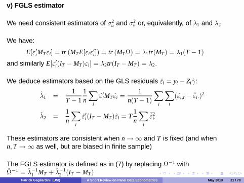
v) FGLS estimator

We need consistent estimators of σ2u and σ2

v or, equivalently, of λ1 and λ2

We have:

E[ε′iMTεi] = tr (MTE[εiε′i]) = tr (MTΩ) = λ1tr(MT) = λ1(T − 1)

and similarly E[ε′i(IT − MT)εi] = λ2tr(IT − MT) = λ2.

We deduce estimators based on the GLS residuals εi = yi − Ziγ:

λ1 =1

T − 11n

∑i

ε′iMT εi =1

n(T − 1)

∑i

∑t

(εi,t − ¯εi·)2

λ2 =1n

∑i

ε′i(IT − MT)εi = T1n

∑i

¯ε2i·

These estimators are consistent when n → ∞ and T is fixed (and whenn, T → ∞ as well, but are biased in finite sample)

The FGLS estimator is defined as in (7) by replacing Ω−1 withΩ−1 = λ−1

1 MT + λ−12 (IT − MT)


The estimators λ1 and λ2 can be used to get estimators of the error variancesσ2

u and σ2v by solving the equations λ1 = σ2

v and λ2 = Tσ2u + σ2

v , namely:

σ2v = λ1, σ2

u =1T

(λ2 − λ1

)

A drawback of estimator σ2u is that it can provide a negative estimated

variance of the individual random effect

Gourieroux, Holly, Monfort (1981, 1982) provide an estimator of σ2u that

ensure positivity


1.4 FIXED EFFECTS OR RANDOM EFFECTS?

A delicate question!

The choice depends on the characteristics of the sample, the interpretation ofthe individual effects, the purpose of the model, etc. For instance:

If the sample contains all the individuals of the underlying population (e.g.the 26 Swiss Cantons), the fixed effects specification appears morenatural

If we are interested in the coefficient of a time-invariant explanatoryvariable, the fixed effects estimator cannot be used


If the model is used to predict the behaviour of an individual with givenobservable characteristics and average unobservable characteristics

E[g(yi,t)|xi,t],

the individual effect has to be integrated out and a random effectsspecification can be used:

E[g(yi,t)|xi,t] =∫

E[g(yi,t)|xi,t, ui]h(ui)dui

where h is the pdf of the individual effect

...


In many economic applications, the sampling scheme is such that theindividual effects can be considered as genuinely random

Then, it is customary to distinguish:

i) Fixed effects approach: no assumptions on distributional properties ofthe individual effects, in particular on the link with explanatory variables

ii) Random effects approach: explicit modeling of the distribution of theindividual effects and their link with regressors


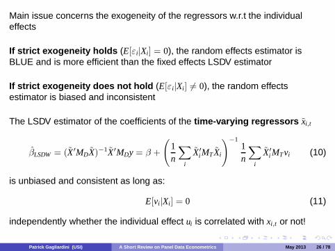
Main issue concerns the exogeneity of the regressors w.r.t the individualeffects

If strict exogeneity holds (E[εi|Xi] = 0), the random effects estimator isBLUE and is more efficient than the fixed effects LSDV estimator

If strict exogeneity does not hold (E[εi|Xi] �= 0), the random effectsestimator is biased and inconsistent

The LSDV estimator of the coefficients of the time-varying regressors xi,t

βLSDW = (X′MDX)−1X′MDy = β +

(1n

∑i

X′i MTXi

)−11n

∑i

X′i MTvi (10)

is unbiased and consistent as long as:

E[vi|Xi] = 0 (11)

independently whether the individual effect ui is correlated with xi,t or not!


A specification test for the null hypothesis of strict exogeneity of theregressors:

H0 : E[εi|Xi] = 0

can be based on the difference

βLSDV − βRE

between the LSDV estimator βLSDV and the random effects estimator βRE ofthe coefficients of the time-varying explanatory variables (Hausman (1978))

Since the random effects estimator βRE is efficient under the null hypothesisH0 of strict exogeneity, we have V[βLSDV − βRE] = V[βLSDV ] − V[βRE]

The Hausman test statistic

ξH = (βLSDV − βRE)′(

V[βLSDV ] − V[βRE])−1

(βLSDV − βRE)

is distributed asymptotically as χ2m under H0, where m is the number of

time-varying explanatory variables


2. IV ESTIMATION OF LINEAR DYNAMIC PANEL DATA MODELS


2.1 INCONSISTENCY OF THE LSDV ESTIMATOR IN LINEAR DYNAMICPANELS

i) The dynamic linear panel data model:

yi,t = αyi,t−1 + ui + vi,t

where:

A.1: The errors vi,t are i.i.d. across individuals and time dates with E[vi,t] = 0and V[vi,t] = σ2

v , for all i and t

A.2: The ui are individual fixed effects

A.3: The initial observations yi,0 are i.i.d. across individuals and independentof the errors vi,t, for all i and t ≥ 1

Compact form: for individual i

yiT×1

= αyi,−1T×1

+ ui STT×1

+ viT×1

where yi,−1 ≡ (yi,0, yi,1, ..., yi,T−1)′


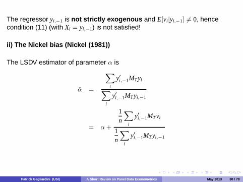
The regressor yi,−1 is not strictly exogenous and E[vi|yi,−1] �= 0, hencecondition (11) (with Xi = yi,−1) is not satisfied!

ii) The Nickel bias (Nickel (1981))

The LSDV estimator of parameter α is

α =

∑i

y′i,−1MTyi∑i

y′i,−1MTyi,−1

= α +

1n

∑i

y′i,−1MTvi

1n

∑i

y′i,−1MTyi,−1


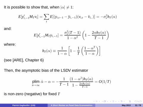
It is possible to show that, when |α| �= 1:

E[y′i,−1MTvi] =∑

t

E[(yi,t−1 − yi,−1)(vi,t − vi,.)] = −σ2v hT(α)

and:

E[y′i,−1MTyi,−1] =σ2

v (T − 1)1 − α2

(1 − 2αhT(α)

T − 1

)where:

hT(α) ≡ 11 − α

[1 − 1

T

(1 − αT

1 − α

)](see [ARE], Chapter 6)

Then, the asymptotic bias of the LSDV estimator

plimn→∞

α − α = − 1T − 1

(1 − α2)hT(α)

1 − 2αhT (α)T−1

= O(1/T)

is non-zero (negative) for fixed T


0 0.1 0.2 0.3 0.4 0.5 0.6 0.7 0.8 0.9 1−0.5

−0.45

−0.4

−0.35

−0.3

−0.25

−0.2

−0.15

−0.1

−0.05

0

α

Bias

T = 5

T = 10

T = 50

T = 20


2.2 INSTRUMENTAL VARIABLE (IV) ESTIMATION

i) The orthogonality restrictions

Write the model in first-differences to eliminate the individual effects

Δyi,t = αΔyi,t−1 + Δvi,t, t = 2, ..., T

where Δyi,t = yi,t − yi,t−1 and Δvi,t = vi,t − vi,t−1

We have a set of m = T(T − 1)/2 orthogonality restrictions for each individual

E[yt−2i (Δyi,t − αΔyi,t−1)] = 0, t = 2, ..., T

where yt−2i ≡ (yi,0, yi,1, ..., yi,t−2)′


The orthogonality restrictions can be written as:

E[Z′i (Δyi − αΔyi,−1)] = 0

where Δyi = (Δyi,2, ..., Δyi,T)′, Δyi,−1 = (Δyi,1, ..., Δyi,T−1)′ and Zi is the(T − 1) × m matrix such that

Zi =

⎛⎜⎜⎜⎝yi,0 0 0 · · · 0 · · · 00 yi,0 yi,1 0 · · · 0...

. . ....

0 0 0 · · · yi,0 · · · yi,T−2

⎞⎟⎟⎟⎠


ii) The GMM (IV) estimator:

αGMM = arg minα

(Δy − αΔy−1)′ZΩZ′(Δy − αΔy−1)

= (Δy′−1ZΩZ′Δy−1)−1Δy′−1ZΩZ′Δy

where Z′Δy ≡∑

i

Z′i Δyi and Ω is a positive definite m × m weighting matrix

(see [ARE])

iii) The optimal weighting matrix: is Ω = V−1, where

V = E[Z′i (Δyi − αΔyi,−1)(Δyi − αΔyi,−1)′Zi] = E[Z′

iΔviΔv′iZi]


iv) The two-step efficient GMM estimator: uses the weighting matrixΩ = V−1 where

V =1n

∑i

Z′i ΔviΔvi

′Zi

with Δvi = Δyi − αΔyi,−1 and α is a consistent first-step GMM estimator of α

The two-step efficient GMM estimator is asymptotically normal (see [ARE]):

√n (αGMM − α) d→ N(0, Σ)

when n → ∞ and T is fixed, where

Σ =(E[Δy′i,−1Zi]V−1E[Z′

iΔyi,−1])−1

Asymptotically valid standard errors and confidence intervals from

AsVar(αGMM) =1nΣ =

⎡⎣(∑i

Δy′i,−1Zi

)(∑i

Z′i ΔviΔvi

′Zi

)−1(∑i

Z′iΔyi,−1

)⎤⎦−1


2.3 PANEL MODELS WITH BOTH STRICTLY EXOGENOUS AND LAGGEDDEPENDENT VARIABLES

Consider the model

yi,t = αyi,t−1 + x′i,tβ + ui + vi,t

= w′i,tγ + ui + vi,t

where wi,t = (yi,t−1, x′i,t)′ and γ = (α, β′)′

⇐⇒ yi = αyi,−1 + Xiβ + uiST + vi = Wiγ + uiST + vi

We add to assumptions A.1-A.3

A.4: The regressor xi,t and the idiosyncratic error vj,s are independent, for anyi, j, t and s (which implies strict exogeneity E[vi|Xi] = 0)


Write the model in first-differences to eliminate the individual effects

Δyi,t = αΔyi,t−1 + Δx′i,tβ + Δvi,t

We have the orthogonality restrictions

E[zi,t(Δyi,t − αΔyi,t−1 − Δx′i,tβ)] = 0, t = 2, ..., T, (12)

where the vector of instruments is:

- zi,t = (yi,t−2, Δx′i,t)′ in Anderson, Hsiao (1981, 1982)

- zi,t = (yi,0, yi,1, ..., yi,t−2, Δx′i,t)′ in Holtz-Eakin, Newey, Rosen (1988),

Arellano, Bond (1991)(may include also lags or leads of Δxi,t)


The Arellano-Bond (1991) GMM estimator:

γGMM =(ΔW ′ZV−1Z′ΔW

)−1ΔW ′ZV−1Z′Δy

where ΔW ′Z ≡∑

i

ΔW ′i Zi and Z′Δy ≡

∑i

Z′iΔyi, with ΔWi = (Δyi,−1, ΔXi)

and

Zi =

⎛⎜⎜⎜⎝yi,0 Δxi,2 0 0 0 · · · 0 · · · 0 00 0 yi,0 yi,1 Δxi,3 · · · 0 · · · 0 0...

.... . .

...0 0 0 0 0 · · · yi,0 · · · yi,T−2 Δxi,T

⎞⎟⎟⎟⎠the optimal weighting matrix V−1 is such that V =

1n

∑i

Z′i ΔviΔv

′iZi, with

Δvi = Δyi − αΔyi,−1 − ΔXiβ and (α, β′)′ is a first-step GMM estimatorobtained with an identity weighting matrix


Remark 1: When the errors vi,t are serially correlated, in general

E[yi,s(Δyi,t − αΔyi,t−1 − Δx′i,tβ)] �= 0

⇒ The lagged endogenous variables up to t − 2 cannot be used asinstruments for Δyi,t−1!

However, the strictly exogenous regressors can still be used as instruments toget the orthogonality restrictions

E[Δxi,s(Δyi,t − αΔyi,t−1 − Δx′i,tβ)] = 0, s = 1, ..., T, t = 2, ..., T

Remark 2: If we only assume that xi,s and vi,t are uncorrelated for s ≤ t, theorthogonality restrictions are:

E[Δxi,s(Δyi,t − αΔyi,t−1 − Δx′i,tβ)] = 0, s = 1, ..., t − 1, t = 2, ..., T


Remark 3: When instruments z∗i are available, which are uncorrelated withthe individual effects, the set of orthogonality restrictions (12) can beextended to include moment restrictions in level

E[z∗i (yi· − αyi,−1 − x′i·β] = 0

⇒ Arellano, Bover (1995) GMM estimator


Remark 4: Blundell, Bond (1998) suggest the use of additional momentrestrictions that are very informative when individual histories are persistent(α close to 1)

Consider the equations:

E[Δyi,t−1εi,t] = 0, t = 3, 4, ..., T, (13)

where εi,t = ui + vi,t, and for t = 2:

E[Δyi,1εi,2] = 0 (14)

Equation (13) is valid under assumptions A.1-A.4, equation (14) is valid underassumptions A.1-A.4 if in addition Cov(yi,0 − ui

1 − α, ui) = 0

Equations (13) and (14) imply moment conditions with instruments indifference for data in level:

E[Δyi,t−1(yi,t − αyi,t−1 − x′i,tβ)] = 0, t = 2, 3, ..., T


Remark 5: a) The number of orthogonality restrictions can be rather largeeven for a short panel and grows with sample size as O(T2)

For instance, with T = 5 periods and K = 5 regressors, in Arellano, Bond(1991) we have T(T − 1)/2 + K(T − 1) = 30 orthogonality restrictions!

b) Some instruments might be “weak”, i.e. weakly correlated with theexplanatory variables

a) & b) cause poor finite-sample performance of standard GMM inferenceprocedures; see e.g. Newey, Windmeijer (2009) for the use of modified GMMestimators


3. NONLINEAR PANEL DATA MODELS


3.1 DISCRETE CHOICE MODELS WITH RANDOM EFFECTS

i) Random utility model

Consider panel data for a binary variable, for instance transportation mode

yi,t ={

0, private (car, motorcycle, ...)1, public (train, bus, ...)

How to model this discrete choice?

Unobservable random utilities from the two alternatives

U0,it = 0, (by normalization)

U1,it = x′i,tβ + εi,t

The observed choice is

yi,t ={

1, if U1,it ≥ U0,it = 00, otherwise


Assume the error component structure

εi,t = ui + vi,t

where individual effects ui ∼ IIN(0, σ2u) and shocks vi,t ∼ IIN(0, σ2

v ) areindependent of each other and of regressors xi,t

Identification constraint: By using εi,t ∼ N(0, σ2u + σ2

v )

P [yi,t = 1|xi,t] = P[εi,t ≥ −x′i,tβ|xi,t

]= Φ

(x′i,tβ√σ2

u + σ2v

)

⇒ parameters are identifiable up to a scale and we can set σ2v = 1

Probability of alternative yi,t = 1 given observable characteristics andindividual effect:

P [yi,t = 1|xi,t, ui] = P[vi,t ≥ −x′i,tβ − ui|xi,t, ui

]= Φ

(x′i,tβ + ui)


ii) General specification

yi,t = 1{

x′i,tβ + ui + vi,t ≥ 0}

A.1: The idiosyncractic errors vi,t are i.i.d. across i and t, independent fromregressors xi = (x′i,1, ..., x′i,T)′, and −vi,t has c.d.f. F

Probability of alternative yi,t = 1 given observable characteristics andindividual effects:

P [yi,t = 1|xi, ui] = P[−vi,t ≤ x′i,tβ + ui|xi, ui] = F(x′i,tβ + ui)

Probit model when F(v) = Φ(v) and logit model when F(v) =1

1 + e−v

A.2: The random individual effects ui are assumed independent of theregressors xi (strict exogeneity) and of errors vi, are i.i.d. acrossindividuals and distributed according to a p.d.f. h(ui; δ) indexed byunknown parameter δ

Parameters of interest are β and δPatrick Gagliardini (USI) A Short Review on Panel Data Econometrics May 2013 47 / 78

iii) The likelihood function

The pdf of observation yi,t given xi = (x′i,1, x′i,2, ..., x′i,T)′ and the random effect ui

f (yi,t|xi, ui; β) = F(x′i,tβ + ui

)yi,t [1 − F(x′i,tβ + ui

)]1−yi,t

By the independence of the individual observations over time conditional onregressors xi and random effect ui, the pdf of vector yi = (yi,1, yi,2, ..., yi,T)′

given xi and ui is

f (yi|xi, ui; β) =T∏

t=1

F(x′i,tβ + ui


)]1−yi,t (15)

We integrate out the random effects and get the pdf of yi given xi

f (yi|xi; β, δ) =∫ (

T∏t=1

F(x′i,tβ + ui


)]1−yi,t

)h(ui; δ)dui


By the independence across individuals, the pdf of vector y = (y′1, y′2, ..., y′n)′

given x = (x′1, x′2, ..., x′n)′ is

f (y|x; β, δ) =n∏

i=1

∫ (T∏

t=1

F(x′i,tβ + ui


)]1−yi,t

)h(ui; δ)dui

We get the log-likelihood function:

Ln,T(β, δ) = log f (y|x; β; δ)

=n∑

i=1

log∫ (

T∏t=1

F(x′i,tβ + ui


)]1−yi,t

)h(ui; δ)dui


iv) The Maximum Likelihood (ML) estimator: is defined by

(β′, δ′)′ = arg maxβ,δ

Ln,T(β, δ)

The ML estimators β and δ are root-n consistent and asymptotically normalwhen n → ∞ and T is fixed:

√n[(β′, δ′)′ − (β′, δ′)′] d→ N(0, I−1),

where I is the Fisher information matrix:

I = E

[−∂2 log f (yi|xi; β, δ)

∂(β′, δ′)′∂(β′, δ′)

].


v) Numerical computation of the ML estimator

Evaluation of the likelihood function for given parameter values requiresnumerical computation of the n one-dimensional integrals∫ (

T∏t=1

F(x′i,tβ + ui


)]1−yi,t

)h(ui; δ)dui

for i = 1, ..., n

Such a numerical approximation is required at each step of the iterativeoptimization algorithm used to get the ML estimates

In a probit model with Gaussian distributed random effects, the integral w.r.t.

the Gaussian pdf h(ui; σ2u) =

1σu

φ

(ui

σu

)can be well approximated by

Gaussian quadrature (Butler, Moffitt (1982))

For more complicated distributions of the random effects, an alternative is toapproximate the integral by Monte-Carlo simulation, which gives aSimulated Maximum Likelihood (SML) estimator (see Gourieroux, Monfort(1993))


3.2 DISCRETE CHOICE MODELS WITH FIXED EFFECTS

i) The modelyi,t = 1

{x′i,tβ + ui + vi,t ≥ 0

}with assumption A.1 of Section 3.1 ii)

The conditional probability of alternative yi,t = 1 is given by:

P[yi,t = 1|xi, ui] = F(x′i,tβ + ui)

where F is the c.d.f. of −vi,t

On the contrary of Section 3.1, here the individual effect ui is not necessarilyindependent of the regressor xi, i.e. we don’t impose assumption A.2

We treat the individual effects ui, for i = 1, ..., n, as parameters to estimate

By taking the log in (15) and summing over i, the log-likelihood function is:

LnT(β, u1, ..., un) =∑

i

∑t

{yi,t log F(x′i,tβ + ui) + (1 − yi,t) log[1 − F(x′i,tβ + ui)]

}(16)


ii) Inconsistency of the ML estimator and incidental parameters problem

It turns out that the ML estimator of parameter β obtained by maximizing thelog-likelihood function (16) is inconsistent for n → ∞ and T fixed!

We illustrate this fact in a “simple” example: F(v) = 1/(1 + e−v) (logit), T = 2periods, xi,1 = 0 and xi,2 = 1 for all i (see [HSI], Section 7.3.1)

The log-likelihood function (16) becomes:

LnT(β, u1, ..., un) =∑

i

[yi,1ui − log(1 + eui) + yi,2(β + ui) − log(1 + eβ+ui)

]By maximizing the log-likelihood w.r.t. the ui for given β, and plugging in LnT

the optimal values ui(β), we get the concentrated log-likelihood of β:

LcnT(β) =

∑i

1{yi,1 + yi,2 = 1}[βyi,2 − β

2− log(1 + e−β/2) − log(1 + eβ/2)

]


By maximizing this concentrated log-likelihood w.r.t. β, we get the MLestimator βML of parameter β

βML = 2 log

(π

1 − π

), π =

∑i 1{yi,1 = 0, yi,2 = 1}∑

i 1{yi,1 + yi,2 = 1}

The Law of Large Numbers (LLN) implies that

plimn→∞

π =P(yi,1 = 0, yi,2 = 1)P(yi,1 + yi,2 = 1)

=1

1 + e−β

We deduce that the ML estimator of β is such that

plimn→∞

βML = 2β

that is, the ML estimator is inconsistent!


The inconsistency of βML is a manifestation of a more general fact called theincidental parameters problem (Neyman, Scott (1948))

The ML estimator of a parameter can be inconsistent when the number ofparameters in the likelihood function grows with the sample size

The individual fixed effects are incidental parameters!

In linear panel models, the incidental parameter problem does not causeinconsistency of the ML estimator of the common parameter (i.e. the LSDVestimator)

In nonlinear panel models, fixed-T inconsistency of the fixed-effects MLestimator due to the incidental parameter problem is pervasive!


iii) The Conditional ML estimator in the panel logit model

For the logit specification, i.e. F(v) = 1/(1 + e−v), a consistent estimator of βis obtained by maximizing a conditional likelihood function given awell-chosen sufficient statistic (Chamberlain (1980))

Let us first consider the case T = 2 to get the intuition

For individual i, let us condition on the event yi,1 + yi,2 = 1. Then:

P[yi,2 = 1|xi, yi,1 + yi,2 = 1] =P[yi,1 = 0, yi,2 = 1|xi]

P[yi,1 = 0, yi,2 = 1|xi] + P[yi,1 = 1, yi,2 = 0|xi]

=ex′i,2β

ex′i,1β + ex′i,2β= F(Δx′i,2β)

with Δxi,2 = xi,2 − xi,1, is independent of ui!

Parameter β can be consistently estimated by running a logit regression onthe subsample of individuals with yi,1 + yi,2 = 1


Extension to T > 2: The p.d.f. of yi = (yi,1, ..., yi,T)′ conditional on

xi = (x′i,1, ..., x′i,T)′ and∑

t

yi,t is

f

(yi|xi,

∑t

yi,t

)∝ exp

(∑t yi,tx′i,tβ

)∑d∈Bi

exp(∑

t dtx′i,tβ)

where Bi denotes the set of vectors d = (d1, ..., dT) ∈ {0, 1}T such that∑t

dt =∑

t

yi,t

The Conditional Maximum Likelihood (CML) estimator:

βCML = arg maxβ

∑i

log

(exp

(∑t yi,tx′i,tβ

)∑d∈Bi

exp(∑

t dtx′i,tβ))

is consistent when n → ∞ and T is fixed


iv) Fixed effects estimators with other error distributions

For the fixed effects probit model, a consistent CML estimator is not available

The Manski (1987) maximum score estimator is a semi-parametricestimator that can be used with a generic distribution of the idiosyncratic errorterms

β = arg maxβ

∑i

∑s<t

sign(yit − yis)sign ((xit − xis)′β)

The intuition is to get the β such that the association

yit > yis ⇔ x′itβ > x′isβ

is maximized across pairs of dates t > s


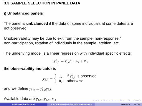
3.3 SAMPLE SELECTION IN PANEL DATA

i) Unbalanced panels

The panel is unbalanced if the data of some individuals at some dates arenot observed

Unobservability may be due to exit from the sample, non-response /non-participation, rotation of individuals in the sample, attrition, etc

The underlying model is a linear regression with individual specific effects

y∗1,it = x′i,tβ + ui + vi,t

the observability indicator is

y2,it ={

1, if y∗1,it is observed0, otherwise

and we define y1,it ≡ y∗1,ity2,it

Available data are y1,it, y2,it, xi,t


ii) The missing-at-random assumption

When does partial unobservability create a bias? When not?

Consider the LSDV estimator computed with the available observations

β =

[∑i

∑t

y2,it(xi,t − xi,·)(xi,t − xi,·)′]−1∑

i

∑t

y2,it(xi,t − xi,·)(y1,it − y1,i·)

= β +

[1n

∑i

∑t

y2,it(xi,t − xi,·)(xi,t − xi,·)′]−1

1n

∑i

∑t

y2,it(xi,t − xi,·)(vi,t − vi,·)

where xi,· ≡ 1Ti

∑t

y2,itxi,t, y1,i· ≡ 1Ti

∑t

y2,ity1,it and Ti ≡∑

t

y2,it

The LSDV estimator is unbiased, and consistent for n → ∞ and T fixed, if:

E[vi|Xi, y2,i] = 0 (17)

Condition (17) is satisfied if E[vi|Xi] = 0 (see (11)) and the mixing-at-randomassumption holds: y2,i and vi are independent, conditional on Xi


iii) Sample selection

Sample selection bias: When individuals elect to drop in/out of the sample,condition (17) is typically not satisfied and the LSDV estimator is inconsistent!

Type 2 Tobit panel model: The selection/observability mechanism ismodeled via a discrete choice

y∗1,it = x′i,tβ + ui + vi,t

y2,it = 1{

z′i,tγ + ηi + wi,t ≥ 0}

y1,it = y∗1,ity2,it

where ηi is the individual specific effect in the selection equation

The econometrician observes y1,it, y2,it, xi,t


iv) Random effects estimator

Model the joint distribution of the individual random effects, idiosyncratic errorterms and regressors

A.1: (ui, ηi) is jointly distributed according to a p.d.f. h(ui, ηi; δ) with unknownparameter δ, e.g. a bivariate Gaussian

A.2: (vi,t, wi,t)′ are i.i.d. across time dates with Gaussian distribution

N

([00

],

[σ2

v ρσv

ρσv 1

])A.3: (ui, ηi), (vi, wi), Xi and Zi are mutually independent and i.i.d. across

individuals

Assumption A.3 implies strict exogeneity of the regressors!

Let us construct the likelihood function. From standard Tobit 2 model:

f (y1,it, y2,it|Xi, Zi, ui, ηi) =[1 − Φ(z′i,tγ + ηi)

]1−y2,it

·⎡⎣ 1

σvφ

(y1,it − x′i,tβ − ui

σv

)Φ

⎛⎝ z′i,tγ + ηi + ρy1,it−x′i,tβ−ui

σv√1 − ρ2

⎞⎠⎤⎦y2,it


By aggregating over time and integrating out the individual effects we get:

f (y1,i, y2,i|Xi, Zi) =∫ ∏

t

([1 − Φ(z′i,tγ + ηi)

]1−y2,it

⎡⎣ 1σv

φ


σv

)Φ


σv√1 − ρ2

⎞⎠⎤⎦y2,it⎞⎠ h(ui, ηi; δ)duidηi

We get the log-likelihood function:

LnT(β, γ, δ, σ2v ) =

∑i

log

{∫ ∏t

([1 − Φ(z′i,tγ + ηi)

]1−y2,it

⎡⎣ 1σv

φ


σv

)Φ


σv√1 − ρ2

⎞⎠⎤⎦y2,it⎞⎠ h(ui, ηi; δ)duidηi

⎫⎬⎭


The random effects ML estimator:

(β, γ, δ, σ2v ) = arg max

(β,γ,δ,σ2v)

LnT(β, γ, δ, σ2v )

is root-n consistent and asymptotically normal when n → ∞ and T is fixed

The evaluation of the log-likelihood for given parameter values requires thenumerical computation of the bivariate integral w.r.t. the individual randomeffects


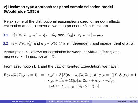
v) Heckman-type approach for panel sample selection model(Wooldridge (1995))

Relax some of the distributional assumptions used for random effectsestimation and implement a two-step procedure a la Heckman

B.1: E[ui|Xi, Zi, ηi, wi] = x′iπ + θηi and E[vit|Xi, Zi, ηi, wi] = ρwit

B.2: ηi ∼ N(0, σ2η) and wi,t ∼ N(0, 1) are independent, and independent of Xi, Zi

Assumption B.1 allows for correlation between individual effect ui andregressor xi. In practice xi = xi,·

From assumption B.1 and the Law of Iterated Expectation, we have:

E[y1,it|Xi, Zi, y2,it = 1] = x′i,tβ + E [E(ui + vi,t|Xi, Zi, ηi, wi, y2,it = 1)|Xi, Zi, y2,it = 1]= x′i,tβ + x′iπ + θE[ηi|Xi, Zi, ηi + wi,t > −z′i,tγ]

+ρE[wit|Xi, Zi, ηi + wi,t > −z′i,tγ]


From assumption B.2 we get:

E[ηi|Xi, Zi, ηi + wi,t > −z′i,tγ] =σ2

η

1 + σ2η

E[ηi + wi,t|Xi, Zi, ηi + wi,t > −z′i,tγ]

=σ2

η

1 + σ2η

λ

⎛⎝− 1√1 + σ2

η

z′i,tγ

⎞⎠where λ(v) =

φ(v)1 − Φ(v)

is the inverse Mill’s ratio

Similarly

E[wit|Xi, Zi, ηi + wi,t > −z′i,tγ] =1

1 + σ2η

λ

⎛⎝− 1√1 + σ2

η

z′i,tγ

⎞⎠

We get:

E[y1,it|Xi, Zi, y2,it = 1] = x′i,tβ + x′iπ +θσ2

η + ρ

1 + σ2η

λ

⎛⎝− 1√1 + σ2

η

z′i,tγ

⎞⎠Patrick Gagliardini (USI) A Short Review on Panel Data Econometrics May 2013 66 / 78

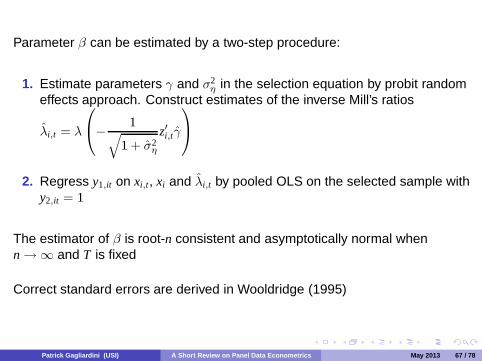
Parameter β can be estimated by a two-step procedure:

1. Estimate parameters γ and σ2η in the selection equation by probit random

effects approach. Construct estimates of the inverse Mill’s ratios

λi,t = λ

⎛⎝− 1√1 + σ2

η

z′i,tγ

⎞⎠2. Regress y1,it on xi,t, xi and λi,t by pooled OLS on the selected sample with

y2,it = 1

The estimator of β is root-n consistent and asymptotically normal whenn → ∞ and T is fixed

Correct standard errors are derived in Wooldridge (1995)


vi) Fixed effects estimator (Kyriazidou (1997))

A mild “stationarity” assumption on the idiosyncratic error terms

C.1: For any two dates t �= s, vectors (vi,t, wi,t, vi,s, wi,s) and (vi,s, wi,s, vi,t, wi,t)are identically distributed conditionally on ξi ≡ (xi,t, zi,t, xi,s, zi,s, ui, ηi)

Under C.1, for any two dates t �= s and an individual i such that z′i,tγ = z′i,sγ

λi,t ≡ E[vi,t|wi,t > −z′i,tγ − ηi, wi,s > −z′i,sγ − ηi, ξi]= E[vi,s|wi,s > −z′i,tγ − ηi, wi,t > −z′i,sγ − ηi, ξi]

= E[vi,s|wi,s > −z′i,sγ − ηi, wi,t > −z′i,tγ − ηi, ξi] = λi,s

⇒ Considering two dates t �= s for which data of individual i are observed andz′i,tγ = z′i,sγ, first-differenting eliminates both the fixed effect and the sampleselection effect!


A two-step estimation procedure:

1. Get an estimator γ of the parameter in the selection equation by a fixedeffects methodology

2. The fixed effects estimator of parameter β is:

β =

[∑i

∑t>s

y2,ity2,is(xi,t − xi,s)(xi,t − xi,s)′K(

(xi,t − xi,s)′γhn

)]−1

·[∑

i

∑t>s

y2,ity2,is(xi,t − xi,s)(y1,it − y1,is)K(

(xi,t − xi,s)′γhn

)]

where K is a kernel and hn > 0 is a bandwidth that shrinks to zero as nincreases

The estimator β is consistent and asymptotically normal when n → ∞ and T isfixed, with non-parametric convergence rate

√nhn

The low convergence rate of this estimator is the cost for the weakassumptions imposed on the error terms


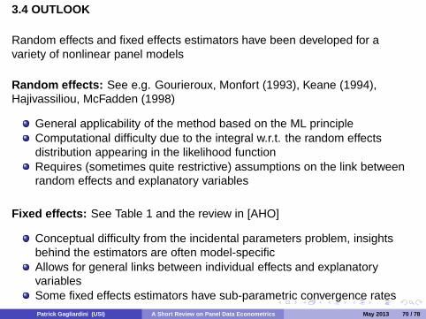
3.4 OUTLOOK

Random effects and fixed effects estimators have been developed for avariety of nonlinear panel models

Random effects: See e.g. Gourieroux, Monfort (1993), Keane (1994),Hajivassiliou, McFadden (1998)

General applicability of the method based on the ML principleComputational difficulty due to the integral w.r.t. the random effectsdistribution appearing in the likelihood functionRequires (sometimes quite restrictive) assumptions on the link betweenrandom effects and explanatory variables

Fixed effects: See Table 1 and the review in [AHO]

Conceptual difficulty from the incidental parameters problem, insightsbehind the estimators are often model-specificAllows for general links between individual effects and explanatoryvariablesSome fixed effects estimators have sub-parametric convergence ratesPatrick Gagliardini (USI) A Short Review on Panel Data Econometrics May 2013 70 / 78

Table 1: Some fixed effects estimators for nonlinear panel models

Discrete choiceLogit, multinomial logit CML, Chamberlain (1980)Semi-parametric Maximum score, Manski (1987)

Tobit modelsCensored regression (Type 1) Honore (1992)Selection model (Type 2) Kyriazidou (1997)Type 3 Honore, Kyriazidou (2000a)

Dynamic modelsDynamic logit Honore, Kyriazidou (2000b)Dynamic censored regression Honore, Hu (2004)Dynamic sample selection Kyriazidou (2001)


Recently, much research considering the fixed-T inconsistency of the fixedeffects ML estimator from the view point of a large-T bias expansion:

E[β] = β +1T

B + O

(1T2

)

Bias adjusted estimators are obtained by eliminating the bias at orderO(1/T), e.g. by analytical methods:

βadj = β − 1T

B

or by jackknife (see e.g. Hahn, Kuersteiner (2002), Hahn, Newey (2004),Dhaene, Jochmans, Thuysbaert (2006), Arellano, Bonhomme (2009),Fernandez-Val (2009))

While fixed-T consistency in not achieved, bias reduction can substantiallyimprove the small-T properties of the fixed effects ML estimator. Moreover,the methodology has general applicability


REFERENCES

A) Books and review chapters

ARE Arellano, M. (2003): Panel Data Econometrics, Advanced Texts inEconometrics, Oxford University Press.

AHO Arellano, M., and B., Honore (2001): Panel Data Models: Some RecentDevelopments, in Handbook of Econometrics, Vol. 5, J. Heckman and E.Leamer (eds), Elsevier, Amsterdam.

CHA Chamberlain, G. (1984): Panel Data, in Handbook of Econometrics, Vol.2, Z. Grilliches and M. Intriligator (eds), Elsevier, Amsterdam.

HSI Hsiao, C. (1986): Analysis of Panel Data, Econometric SocietyMonographs, Cambridge University Press.

MAS Matyas, L., and P., Sevestre (Eds.) (1992): The Econometrics of PanelData. Handbook of Theory and Applications, Advanced Studies inTheoretical and Applied Econometrics, Kluwer Academic Publishers.Patrick Gagliardini (USI) A Short Review on Panel Data Econometrics May 2013 73 / 78

B) Articles

Anderson, T. W., and C., Hsiao (1981): ”Estimation of Dynamic Models withError Components”, Journal of the American Statistical Association, 76,598-606.

Anderson, T. W., and C., Hsiao (1982): ”Formulation and Estimation ofDynamic Models Using Panel Data”, Journal of Econometrics, 18, 47-82.

Arellano, M., and S., Bond (1991): ”Some Tests of Specification for PanelData: Monte Carlo Evidence and an Application to Employment Equations”,Review of Economic Studies, 58, 277-297.

Arellano, M., and S., Bonhomme (2009): “Robust Priors in Nonlinear PanelData Models”, Econometrica, 77, 489-536.

Arellano, M., and O., Bover (1995): ”Another Look at the Instrumental VariableEstimation of Error-Components Models”, Journal of Econometrics, 68, 29-51.

Balestra, P., and M., Nerlove (1966): ”Pooling Cross-Section and Time SeriesData in the Estimation of a Dynamic Model: The Demand for Natural Gas”,Econometrica, 34, 585-612.


Blundell, R., and S., Bond (1998): ”Initial Conditions and Moment Restrictionsin Dynamic Panel Data Models”, Journal of Econometrics, 87, 115-143.

Butler, I., and R., Moffitt (1982): ”A Computationally Efficient QuadratureProcedure for the One-Factor Multinomial Probit Model”, Econometrica, 50,761-764.

Chamberlain, G. (1980): ”Analysis of Covariance with Qualitative Data”,Review of Economic Studies, 47, 225-238.

Dhaene, G., Jochmans, K., and B., Thuysbaert (2006): ”Jackknife BiasReduction for Nonlinear Dynamic Panel Data Models with Fixed Effects”,Working Paper, Leuven University.

Fernandez-Val, I. (2009): ”Fixed Effects Estimation of Structural Parametersand Marginal Effects in Panel Probit Model”, Journal of Econometrics, 150,71-85.

Gourieroux, C., Holly, A., and A. Monfort (1981): ”Kuhn-Tucker, LikelihoodRatio and Wald Tests for Nonlinear Models with Inequality Constraints on theParameters”, Journal of Econometrics, 16, 166.


Gourieroux, C., Holly, A., and A. Monfort (1982): ”Likelihood Ratio Test, WaldTest, and Kuhn-Tucker Test in Linear Models with Inequality Constraints onthe Regression Parameters”, Econometrica, 50, 63-80.

Gourieroux, C., and A. Monfort (1993): ”Simulation Based Inference: ASurvey with Special Reference to Panel Data Models”, Journal ofEconometrics, 59, 5-33.

Hahn, J., and G., Kuersteiner (2002): ”Asymptotically Unbiased Inference fora Dynamic Panel Model with Fixed Effects When Both n and T are Large”,Econometrica, 70, 1639-1657.

Hahn, J., and W., Newey (2004): ”Jackknife and Analytical Bias Reduction forNonlinear Panel Models”, Econometrica, 72, 1295-1319.

Hajivassiliou, V., and D., McFadden (1998): ”The Method of Simulated Scoresfor the Estimation of LDV Models”, Econometrica, 66, 863-896.

Hausman, J. (1978): ”Specification Tests in Econometrics”, Econometrica, 46,1251-1271.

Hoch, I. (1962): ”Estimation of Production Function Parameters CombiningTime Series and Cross-Section Data”, Econometrica, 30, 34-53.


Honore, B. (1992): ”Trimmed LAD and Least Squares Estimation of Truncatedand Censored Regression Models with Fixed Effects”, Econometrica, 60,533-565.

Honore, B., and L., Hu (2004): ”Estimation of Cross-Sectional and Panel DataCensored Regression Models with Endogeneity”, Journal of Econometrics,122, 293-316.

Honore, B., and E., Kyriazidou (2000a): ”Estimation of Tobit-Type Models withIndividual Specific Effects”, Econometric Reviews, 19, 341-366.

Honore, B., and E., Kyriazidou (2000b): ”Panel Data Discrete Choice Modelswith Lagged Dependent Variables”, Econometrica, 68, 839-874.

Holtz-Eakin, D., Newey, W., and H., Rosen (1988): ”Estimating VectorAutoregressions with Panel Data”, Econometrica, 56, 1371-1395.

Keane, M. (1994): ”A Computationally Practical Simulation Estimator for PanelData”, Econometrica, 62, 95-116.

Kyriazidou, E. (1997): ”Estimation of a Panel Data Sample Selection Model”,Econometrica, 65, 1335-1364.


Kyriazidou, E. (2001): ”Estimation of Dynamic Panel Data Sample SelectionModels”, Review of Economic Studies, 68, 543-572.

Manski, C. (1987): ”Semiparametric Analysis of Random Effects LinearModels from Binary Panel Data”, Econometrica, 55, 357-362.

Mundlak, Y. (1961): ”Empirical Production Functions Free of ManagementBias”, Journal of Farm Economics, 43, 69-85.

Mundlak, Y. (1978): ”On the Pooling of Time Series and Cross-Section Data”,Econometrica, 46, 69-85.

Neyman, J., and E., Scott (1948): ”Consistent Estimates Based on PartiallyConsistent Observations”, Econometrica, 16, 1-31.

Newey, W., and F., Windmeijer (2009): ”Generalized Method of Moments withMany Weak Moment Conditions”, Econometrica, 77, 687-719.

Nickel, S. (1981): ”Biases in Dynamic Models with Fixed Effects”,Econometrica, 49, 1417-1426.

Wooldridge, J. (1995): ”Selection Correction for Panel Data Models underConditional Mean Independence Assumptions”, Journal of Econometrics, 68,115-132.


a short review on panel data econometrics

Documents