a simplified approach to condensed phase combustion ... · a simplified approach to condensed phase...
TRANSCRIPT

A Simplified Approach to Condensed Phase Combustion Modeling
Frederick Paquet
A thesis
in
The Department
of
Mechanical and Industrial Engineering
Presented in Partial Fulfillment of the Requirements
for the Degree of Master of Applied Science (Mechanical Engineering) at
Concordia University
Montreal, Quebec, Canada
April 2008
© Frederick Paquet, 2008

1*1 Library and Archives Canada
Published Heritage Branch
395 Wellington Street Ottawa ON K1A0N4 Canada
Bibliotheque et Archives Canada
Direction du Patrimoine de I'edition
395, rue Wellington Ottawa ON K1A0N4 Canada
Your file Votre reference ISBN: 978-0-494-40919-0 Our file Notre reference ISBN: 978-0-494-40919-0
NOTICE: The author has granted a nonexclusive license allowing Library and Archives Canada to reproduce, publish, archive, preserve, conserve, communicate to the public by telecommunication or on the Internet, loan, distribute and sell theses worldwide, for commercial or noncommercial purposes, in microform, paper, electronic and/or any other formats.
AVIS: L'auteur a accorde une licence non exclusive permettant a la Bibliotheque et Archives Canada de reproduire, publier, archiver, sauvegarder, conserver, transmettre au public par telecommunication ou par Plntemet, prefer, distribuer et vendre des theses partout dans le monde, a des fins commerciales ou autres, sur support microforme, papier, electronique et/ou autres formats.
The author retains copyright ownership and moral rights in this thesis. Neither the thesis nor substantial extracts from it may be printed or otherwise reproduced without the author's permission.
L'auteur conserve la propriete du droit d'auteur et des droits moraux qui protege cette these. Ni la these ni des extraits substantiels de celle-ci ne doivent etre imprimes ou autrement reproduits sans son autorisation.
In compliance with the Canadian Privacy Act some supporting forms may have been removed from this thesis.
Conformement a la loi canadienne sur la protection de la vie privee, quelques formulaires secondaires ont ete enleves de cette these.
While these forms may be included in the document page count, their removal does not represent any loss of content from the thesis.
Canada
Bien que ces formulaires aient inclus dans la pagination, il n'y aura aucun contenu manquant.
Abstract
A Simplified Approach to Condensed Phase Modelling
Frederick Paquet
The combustion modeling of energetic materials still involves a guessing step due to the lack
of knowledge in the condensed phase. Quantum dynamical calculations are presently the only
way to predict the initial gasification reaction but require tremendous computing power, thus
limiting their application. This constitutes a lack of completeness in the design of modeling tools.
Through quantum mechanics, it is known that incoming energy will couple only in certain ways
with a molecular system. The way this coupling is defined will depend on the selection of an
energy model. A simple empirical method was devised which uses an energy coupling
assumption and spectroscopic data of energetic molecules as the source for the complete modal
molecular picture of the system. The method enables a qualitative prediction of the first
combustion reaction through comparison with emission spectra of energy sources. The goal of
this work is to present the method developed along with some results and gather tools for
future research in the same subject. The thesis will first review the current state of research in
the field of condensed phase energetic materials combustion. A discussion on the different
theoretical foundations and assumptions used related to quantum mechanics and spectroscopy
shall follow culminating with a description of the method developed. The analysis method will
then be applied with two example energetic molecules nitroguanidine and nitrocellulose. The
study will conclude with an explicit prediction for the two example cases followed by a
discussion on future research that could be undertaken based on the conclusions drawn here.
in

Resume
Une Approche Simplifiee pour la Moderation de la Phase Condensee
Frederick Paquet
La modelisation de la combustion des materiaux energetiques requiere encore une etape de
supposition en raison du manque de connaissance sur la phase condensee. Les calculs appliques
de dynamique quantique sont presentement la seule maniere de predire la reaction initiale de
conversion en gaz mais ces derniers requierent une puissance informatique tres importante.
Cette situation demontre un manque dans la conception des outils de modelisation. La
mecanique quantique nous montre que certains niveaux d'energie tres precis sont absorbes par
un systeme moleculaire. La valeur de ces niveaux depend du type de modele d'energie
potentielle choisis. Une methode empirique simple fut developpee a I'aide d'une hypothese de
couplage de I'energie et de donnees spectroscopiques de molecules energetiques. La
spectroscopie est prise ici comme I'image modale complete d'un systeme moleculaire. La
methode permet une prediction qualitative de la premiere reaction lors d'une combustion par
une comparaison avec les spectres d'emission de differentes sources d'energie. Le but de ce
travail est de presenter la methode avec quelques resultats ainsi que d'acquerir les outils qui
necessaires a la continuation de cette recherche. Cette these revisera premierement I'etat
present de la recherche dans le champ de la combustion en phase condensee. Une discussion
sur les differentes fondations theoriques relevant de la mecanique quantique et de la
spectroscopie suivra et culminera avec une description de la methode proposee. La methode
d'analyse sera par la suite appliquee avec deux molecules energetiques : la nitroguanidine et la
nitrocellulose. Cette etude sera finalement conclue par une prediction de la premiere reaction
des cas utilises en exemple et discutera des contributions futures possibles a cette recherche.
IV

Acknowledgments
First of all, I would like to thank Dr. Hoi Dick Ng, my supervisor, for giving me the
opportunity to complete this project and for providing me with precious help and advice. I
would also like to thank General Dynamics -- Ordinance and Tactical Systems Canada -
Valleyfield for their financial support of this project. I would also like to highlight the
contributions of Mario Paquet, Daniel Lepage, and Stephane Viau for the many interesting
discussions throughout the realization of this project. Finally I would like to thank Christie
Nichols for her continuous support and encouragement.
v

Contents
List of Figures ix
List of Tables xi
Glossary xii
1 Introduction 1
1.1 General overview 1
1.2 Basics of propellant combustion • 2
1.3 Condensed phase combustion 6
1.3.1 Theory and modelling 6
1.3.2 Experimental investigations 9
1.4 Current knowledge about energetic molecules 10
1.4.1 Nitramines 11
1.4.2 Nitrate esters 12
1.4.3 General observations on energetic compounds categories 14
1.5 Objective of the present study 14
VI

Contents
2 Molecular Modes and Spectroscopy 16
2.1 Fundamental concepts and method approach 17
2.2 Assumptions used in the method 17
2.3 The energy coupling assumption 19
2.4 Spectroscopy 21
2.5 Molecular dissociation 26
2.6 Summary 27
3 Application of the Method 29
3.1 General overview 29
3.2 Example: Nitroguanidine 29
3.3 Example: Nitrocellulose 35
3.4 Discussion on the calculations results 39
4 Energy Input Spectrum and Ignition 41
4.1 General overview 41
4.2 Ignition and some possible sources 42
4.3 Input spectrum through emission spectroscopy 43
4.4 Ignition through a temperature rise 46
5 Conlusions 49
5.1 Concluding remarks . 4 9
5.2 Contribution to knowledge 51
vn

Contents
References 52
Appendices 55
viii
List of Figures
1.1 Schematic of the physical phases found in a combustion 3
2.1 Comparison of the quantum harmonic and Morse potential curves 20
2.2 Simplified schematic of a spectrophotometer 22
2.3 Representation of the different forms of vibrational modes 24
3.1 The infrared spectrum of nitroguanidine (Sigma Aldrich Catalog) 30
3.2 Schematic of the nitroguanidine molecule 31
3.3 The ultraviolet spectrum of nitroguanidine 33
3.4 Graphical representation of appended tabular data for the NH2 stretches . . 35
3.5 Schematic of the nitrocellulose molecule 36
3.6 Schematic of the cellulose molecule 37
3.7 First dissociation wavelengths calculated for NQ and NC 39
4.1 Comparison of dissociation wavelengths of NC with the emission spectrum for
JA2 44
4.2 Comparison of dissociation wavelengths of NQ with the general emission spec
trum trend 45
IX

List of Figures
4.3 Fraction of bonds with the dissociation energy (NO2 stretches case) 47
x

List of Tables
3.1 Spectroscopy analysis and calculation results for nitroguanidine 34
3.2 FT-IR spectroscopy peaks wavenumbers values 38
3.3 Spectroscopy analysis and calculation results for nitrocellulose . . . . . . . . 38
xi
Glossary
As
c
E
Ed
Es
h
hi
k
h I
•J
rh
n
nv
R
X
t
T
V
Yi
Z
Pre-exponential constant
Speed of light
Energy
Dissociation energy
Activation energy
Planck's constant
Species enthalpy
Spring constant; Wave number
Boltzmann's constant
Moment of inertia
Rotational quantum number
Gasification rate
Quantum number
Vibrational quantum number
Ideal gas constant
Single dimension of the system
Time
Temperature
Potential energy
Species mass fraction
Partition function
Xll

Acronyms DEGDN
DSC
FTIR
GN
HMX
MURI
NC
NG
NQ
PREMIX
RDX
TAGN
TEGDN
TMETN
TGA
SEM
Diethylene glycol dinitrate
Differential scanning calorimeter
Fourier transform infraRed
Guanidine nitrate
Cyclo-tetramethylene-tetranitramine
Multidisciplinary university research initiative
Nitrocellulose
Nitroglycerine
Nitroguanidine
Chemkin premixed flame code
Cyclo-trimethylene-trinitramine
Triaminoguanidine nitrate
Triethylene glycol dinitrate
Trimethyloletane trinitrate
Thermo-gravimetric analysis
Scanning electron microscopy
Greeks v Frequency
v0 Fundamental frequency
Xg Thermal conductivity
A Wave length
xiii

Chapter 1
Introduction
1.1 General overview
The modern requirements for applications such as rockets, airbags infiators and guns are
changing how new propellants are formulated. Traditional ingredients, such as nitrocellulose
(NC) and nitroglycerine (NG) are no longer able to always provide valid solutions to meet
specifications. In order to modernize propellant formulation, a great deal of research is being
done to discover and test new energetic molecules. In addition, theoretical and empirical
knowledge is being increasingly coupled with the power of computers to predict the burning
behaviour of propellants. In that aspect, the application of gaseous phase chemistry has been
quite successful in representing the reality. However, the gas phase processes correspond often
only the second part of the combustion phenomenon. The beginning of combustion occurs in
the condensed phase of the material in most cases. The reactions occurring in the condensed
phase dictate what could possibly happen in the gas phase. Nowadays, due to a lack of
theoretical and experimental knowledge, the condensed phase reactions are usually derived
from educated guesses (Beckstead, 2006). It has been shown that different condensed phase
reactions can yield very different burning behaviour because of a number of possible reaction
paths (Miller and Anderson, 2000). A theoretical understanding of condensed phase processes
in the combustion of propellants could therefore enable one to design a propellant system
1

Chapter 1. Introduction
that would use a wanted reaction path in order to get a precise defined burning behaviour.
The development of a general method to predict the initial condensed phase decomposition
reaction is the general goal of this research.
1.2 Basics of propellant combustion
One of the most important propellant parameter is its burning rate (usually measured in
units of distance per unit time). Altough the energy content of a given formulation is also an
important parameter, a high energy content does not imply a high burning rate. A good ex
ample of this is the case of RDX (cyclo-trimethylene-trinitramine). While RDX has interesting
thermodynamic properties and a high energy content, its burning rate is fairly low and thus
limits greatly the number of applications in which it can be used with success. The capability
to accurately predict burning rates (or gasification rates) for different propellants has been
one of the main thrusts in the energetic material combustion research effort. It is currently
required to manufacture enough of a given propellant to be able to test it in a closed vessel
and measure the burning rate. This is a costly and time consuming process. Furthermore,
using empirical correlations built by the experience of repeating the above process does not
at all bring a level of understanding comparable to theoretical knowledge.
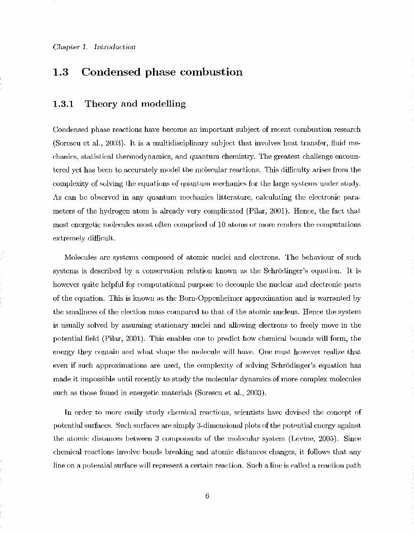
In the last two decades, combustion modelling of propellants has been done using mostly
similar basic steps. The process is divided into three phases: solid, condensed and gaseous
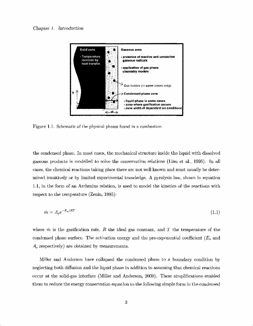
(Beckstead, 2006). This is illustrated in figure 1.1. The conservation relations (mass and
energy) are solved for all three zones and a set of boundary conditions are applied between the
zones. Usually, only the energy equation is solved in the solid phase to model the convection
and conduction heat transfer as no chemical reactions are assumed there (Beckstead, 2006).
In the thin condensed phase zone, the reactants are taken as liquids and gas bubbles are
present due to the gasification process taking place there (Schroeder et al., 2001). Hence
molecular diffusion is an important component and is included in the mass conservation rela
tion. Several modelling philosophies have been used to simulate the processes taking place in
2
Chapter 1. Introduction
Gaseous zone
- presence of reactive and unreactive gaseous radicals
- application of gas phase chemistry models
Gas bubies {in some cases only)
Condensed phase zone
- liquid phase in some cases - zone where gasification occurs - zone width dl dependant on conditions
<-°l-^
Figure 1.1. Schematic of the physical phases found in a combustion
the condensed phase. In most cases, the mechanical structure inside the liquid with dissolved
gaseous products is modelled to solve the conservation relations (Liau et al., 1995). In all
cases, the chemical reactions taking place there are not well known and must usually be deter
mined intuitively or by limited experimental knowledge. A pyrolysis law, shown in equation
1.1, in the form of an Arrhenius relation, is used to model the kinetics of the reactions with
respect to the temperature (Zenin, 1995):
m = A,e~E'/Rr (1.1)
where m is the gasification rate, R the ideal gas constant, and T the temperature of the
condensed phase surface. The activation energy and the pre-exponential coefficient (Es and
As respectively) are obtained by measurements.
Miller and Anderson have collapsed the condensed phase to a boundary condition by
neglecting both diffusion and the liquid phase in addition to assuming that chemical reactions
occur at the solid-gas interface (Miller and Anderson, 2000). These simplifications enabled
them to reduce the energy conservation equation to the following simple form in the condensed
3

Chapter 1. Introduction
phase:
A* ( f ) = ™E (yr\+0 - Y-hr) (i.2)
where Xg is the thermal conductivity of the gas phase, T is the temperature, rh is the gasifica
tion rate (mass of gas produced per unit time), Yi is the mass fraction of the ith species, hi is
the enthalpy of the ith species and x is the single dimension of the system. Note that the super
scripts "-co" and "—0" and "+0" relate to the unreacted propellant, the condensed phase side
of the surface and the gas phase side of the surface respectively. This modelling method by
Miller and Anderson has the virtue of greatly simplifying the condensed phase analysis while
yielding accurate results. The two authors have published results of linear burning rate pre
dictions using their model for single, double and triple base propellants (Miller and Anderson,
2004) containing a variety of widely used energetic materials such as nitrocellulose, nitro
glycerine, nitroguanidine, RDX (Cyclo-trimethylene-trinitramine), and DEGDN (diethylene
glycol dinitrate). Their results were shown to be in agreement with experimental data but
were dependent upon the chosen initial condensed phase reaction (Miller and Anderson, 2000).
Hence the method remains an empirically-based one.
The conservation relations are usually solved using a combustion simulation code such as
PREMIX (Kee et al., 1985). In fact, Miller and Anderson used a modified version of PRE-
MIX as a subroutine in their modelling system (Miller and Anderson, 2000). For propellant
simulations there is a much better understanding of gas phase phenomena during combustion;
this is why the methods used there are more standard.
It appears that modelling the combustion of propellants is not an easy matter due to
the lack of theoretical and experimental understanding of condensed phase processes. There
are many research groups that currently devote their studies to the molecular dynamics of
condensed phase energetic materials combustion. The MURI (Multidisciplinary University
Research Initiative) Accurate Theoretical Predictions of the Properties of Energetic Materials
research group is a good example. The subject however remains very challenging and major
advancements have been limited. Hence, important work should be done to better understand
condensed phase processes during combustion in order to improve the modeling and control
4

Chapter 1. Introduction
the phenomena.
5
Chapter 1. Introduction
1.3 Condensed phase combustion
1.3.1 Theory and modelling
Condensed phase reactions have become an important subject of recent combustion research
(Sorescu et al., 2003). It is a multidisciplinary subject that involves heat transfer, fluid me
chanics, statistical thermodynamics, and quantum chemistry. The greatest challenge encoun
tered yet has been to accurately model the molecular reactions. This difficulty arises from the
complexity of solving the equations of quantum mechanics for the large systems under study.
As can be observed in any quantum mechanics litterature, calculating the electronic para
meters of the hydrogen atom is already very complicated (Pilar, 2001). Hence, the fact that
most energetic molecules most often comprised of 10 atoms or more renders the computations
extremely difficult.
Molecules are systems composed of atomic nuclei and electrons. The behaviour of such
systems is described by a conservation relation known as the Schrodinger's equation. It is
however quite helpful for computational purpose to decouple the nuclear and electronic parts
of the equation. This is known as the Born-Oppenheimer approximation and is warranted by
the smallness of the election mass compared to that of the atomic nucleus. Hence the system
is usually solved by assuming stationary nuclei and allowing electrons to freely move in the
potential field (Pilar, 2001). This enables one to predict how chemical bounds will form, the
energy they contain and what shape the molecule will have. One must however realize that
even if such approximations are used, the complexity of solving Schrodinger's equation has
made it impossible until recently to study the molecular dynamics of more complex molecules
such as those found in energetic materials (Sorescu et al., 2003).
In order to more easily study chemical reactions, scientists have devised the concept of
potential surfaces. Such surfaces are simply 3-dimensional plots of the potential energy against
the atomic distances between 3 components of the molecular system (Levine, 2005). Since
chemical reactions involve bonds breaking and atomic distances changes, it follows that any
line on a potential surface will represent a certain reaction. Such a line is called a reaction path
6

Chapter 1. Introduction
in molecular dynamics (Levine, 2005). If no external forces are present, a reaction will strive
to attain the minimum equilibrium energy possible. One can thus study potential surfaces
of a given energetic material to determine which bound is likely to break first. The limits
of computing power restrict the possible dimensionality of the problem (number of molecular
components that can be studied at the same time). Furthermore, since potential surfaces are
calculated from empirical observations (for an approximation purpose), errors will come from
the particular empirical models chosen (Sorescu et al., 2003).
The methods discussed above are equally valid in the treatment of gas phase or condensed
phase phenomena. In the condensed phase (liquid and/or solid), the structure of the substance
(e.g.: long liquid polymer chains, crystals, etc.) must also be considered as it will influence
its physical properties and how it will absorb energy.
Solids consist of molecules arranged together in a more or less orderly fashion with cohesion
due to the electrostatic force between molecules (not by chemical bounds) (Dlott, 2003).
Given the nature of solids, there are two possible excitation modes possible: translation
and vibration. It is important to differentiate between the processes linked to each of these
modes. It has been reported that shock waves (such as those found in detonations) will
affect the translational modes of the molecules within the solid (Dlott, 2003). This shows the
phenomena to be more of a mechanical energy transfer. In the case of deflagration processes,
the vibrational modes will be exited due to the thermal energy transferred to the unburned
material. Hence it apparently becomes useful to separate shock and thermal energy transfer
causes in the theoretical studies (Dlott, 2003). In the case of propellants, there is strictly
thermal energy transfer (although shock waves are quite possible but extremely unwanted in
this case).
Extensive studies are currently being made to better understand the geometric structure of
solid energetic materials. Knowing the microscopic geometrical shape of these crystals enables
one to calculate the different excitation modes of the material. Early models considered only
rigid molecules and thus neglected intra-molecular vibrations. However, such models are
not useful as they do not describe well the conditions encountered in the high pressures and
7
Chapter 1. Introduction
temperatures characteristic of combustion (Sorescu et al., 2003). In order to better capture the
vibrational behaviour, potential energy surfaces (such as the well known Morse potential) are
used. By combining the knowledge of both inter and intra molecular modes, a more complete
picture of the material under study is obtained. One can then solve the Schrodinger's equation
in a molecular dynamics simulation and determine how the energy input will affect the system
(Dlott, 2003). Again, it must be stressed that such calculations have only recently become
possible to perform with an acceptable precision due to the computing power required.
In the case of liquids, things become more complicated as rotation must be taken into
account. The description of liquids is more difficult as they exhibit properties common to
both gases and solids. It is therefore hard to use approximations that would neglect any of
these important properties (Hill, 1987) and the analysis that is already tedious for the simpler
cases becomes almost impossible for the moment. There would however be a lot to be gained
from a better understanding of liquid state combustion as many energetic materials are used
in a liquid form (such as NG and DEGDN) and a large number of the others are suspected
to decompose after the fusion to their liquid state (Schroeder et al., 2001).
From the above discussion, it becomes clear that the current state of the art condensed
phase theory and modelling is extremely complex. The molecular structures and reactions
are derived directly from pure quantum mechanics by making a few relevant assumptions to
simplify the computations (Sorescu et al., 2003). There is no mention of any simpler theory or
method that would be valid for condensed phase combustion. In other words, this resembles
the case where one would be using the general theory of relativity to launch a spacecraft in
orbit rather then classical mechanics. It would be desirable to search for simpler methods
based on what is already known (which would offer many engineering perspectives). One
can note here the advantage that the more complete and general theory is already known
(compared to the case of classical and relativistic mechanics).
8

Chapter 1. Introduction
1.3.2 Experimental investigations
Although the empirical study of condensed phase combustion processes have always been
deemed as difficult, there have been several interesting studies on the subject. The most
successful methods have been mostly revolving around thermal analysis, spectroscopy and
microscopy. A coupling of these methods with the knowledge of the thermodynamics of the
reactant and possible products enabled researchers to emit some significant hypothesis about
condensed phase reactions.
The physico-chemical study of propellants with a quenched reaction surface using scan
ning electron microscopy (SEM) and Fourier transform infrared (FTIR) microscopy has been
attempted, as shown by a recent string of publications by Schroeder et al. (2001). The visual
SEM analysis enabled the authors to distinguish the different phases that were present at the
time of quenching (liquid, amorphous solid, crystalline solid) in cross sections of the material.
FTIR microscopy produced a spectrum of these sections that could be compared to the spec
trum of unburned material samples and to chemical bounds spectral references. For example,
the appearance of certain bands or the decrease in the amplitude of others in the spectrum is
directly related to the presence of certain chemical groups and bounds. The knowledge of the
groups present at the quenching can be used to determine what intermediate reactions could
have taken place with more precision (Schroeder et al., 2001).
A very interesting and simple approach concerning the decomposition of triaminoguani-
dine nitrate (TAGN) was suggested by Kubota et al. (1988). Their method involved thermo-
gravimetric (TGA) and differential scanning calorimeter (DSC) measurements. The DSC mea
surements showed the phase change from solid to liquid followed by a multi-stage exothermic
decomposition. The TGA measured the mass losses from solid-liquid to gases. Combining
the two measurements gave a serious hint that the main energetic property of TAGN arises
from the initial breakage of the three NH2 bounds. This conclusion comes from the match in
the mass fraction of the amino groups and the mass loss measured by TGA (Kubota et al.,
1988). Comparison with the same measurements done on the brother-substance of TAGN,
guanidine nitrate (GN), and thermodynamical data enabled to reinforce the conclusions of the
9
Chapter 1. Introduction
researchers. Continuing the reaction of a TAGN sample that had its combustion quenched
after the initial amino loss showed the expected resemblance with GN when looking at the
DSC and TGA profiles (Kubota et al., 1988).
It can be seen here that the discussed techniques do not show directly the condensed phase
chemical processes occurring but enable one to deduce what happens. Indeed, there has not
been much success in trying to study the direct products of condensed phase processes due
to the temporary nature of these products and especially the difficult pressure/temperatures
at which they must be measured. Complex apparatus, such as that featured in a study by
Korobeinichev (2000), would present an extremely interesting alternative if it could work in
harsher conditions. The more simple approaches discussed here would however be useful in
verifying future theoretical predictions.
1.4 Current knowledge about energetic molecules
Following the previous general discussions, it is interesting to look at some energetic substances
and what has been discovered about their condensed phase combustion in more details using
the techniques and theorie that have been presented. The conclusions and ideas presented in
this section will serve as a mean of validation to the calculations that shall be made later in
this study with certain energetic molecules. It must be noted again that the initial condensed
phase reactions of different energetic molecules described here are not at all completely proven
as true but are currently regarded as the most probable ones.
Energetic compounds are divided into families based on the structure of their molecules
and the presence of some chemical groups and bonds. All members of these families have
some similar characteristics during their combustion due to the molecular groups common to
them. Two categories that are widely used in propellant formulations, nitramines and nitrate
esters, are further discussed here.
10
Chapter 1. Introduction
1.4.1 Nitramines
The main feature of nitramines is their hydrocarbon-like structure containing several N-NO2
chemical bounds (Kubota, 2007). At standard temperature and pressure, they are in a crys
talline form. Their combustion involves a change of phase to liquid and, to some extent,
gaseous form.
Among the nitramines, cyclo-trimethylene-trinitramine RDX is a widely used substance
in many explosives, propellants and gas generating compositions. Its condensed phase com
bustion is still quite misunderstood even if it has been quite extensively studied. What is
known with certainty is that a burning RDX sample consists of a cool solid propellant zone, a
heating zone still in the solid phase and a liquid phase containing gas bubbles. The length of
this liquid layer decreases with increasing pressures (Schroeder et al., 2001). The composition
of the gas bubbles is not certain and is the main source of the problem. Most researchers now
believe that the bubbles are made of RDX vapour (Miller and Anderson, 2000). Others claim
that they consist more of a mixture of decomposition products and RDX vapour (Schroeder
et al., 2001). This is important as the initial reaction involved to decompose a liquid or a
gas will be different. The main argument used to defend the liquid phase decomposition is
that RDX melts at 204°C, starts decomposing at 227°C and is estimated to boil at 391 + / -
33°C (Schroeder et al, 2001). The vapour phase decomposition hypothesis was applied in the
burning rate prediction model of Miller & Anderson (Miller and Anderson, 2000) with a fairly
good success. The actual chemical decomposition reaction is not known in the liquid phase
for the moment as this process in not favoured by researchers.
Another nitramine is Cyclo-tetramethylene-tetranitramine (HMX). The combustion of
HMX seems to be much more understood then that of RDX as judged by the number of
publications and their clarity. Kubota reports (Kubota, 2007) that the initial decomposition
reaction of HMX is the following:
3(CH2NN02)4 -»• 4N02 + 4N 20 + 6N2 + 12CH20 (R-l)
Differential scanning calorimeter and thermo-gravimetric analysis measurements have shown
11

Chapter 1. Introduction
that this reaction is likely to occur in the liquid phase (Kubota et al., 1989). Furthermore,
FTIR analysis has helped to confirm that the decomposition reaction begins with the breaking
of the N-NO2 bond, thus yielding reaction R-l (Kubota et al., 1989). The condensed phase
again contains gas bubbles with the initial reaction products along with possible further gas-
phase reactions products. Like RDX, the liquid phase layer is shown to decrease in length
with increasing pressure (Schroeder et al., 2001).
The last nitramine discussed is nitroguanidine (NQ), which is a common triple base pro-
pellant ingredient. NQ is a crystalline solid usually used as energetic filler in triple base
propellants because of the low molecular weight of its combustion gases and its low flame
temperature. Most research on this substance tends to favour the breaking of all single bonds
as an initial reaction (Volk, 1985). In their modelling effort, Miller & Anderson have found
that the reaction yielding the best burning rate results is the following (Miller and Anderson,
2004):
NQ(solid) -y N0 2 +HCN+NH 2 +NH (R-2)
Observation of R-2 confirms the. breaking of single bonds. The reaction is assumed to be
occurring in the solid phase as NQ has a melting point of 255° C and a decomposition temper
ature of 250°C (Miller and Anderson, 2004). As seen in R-2, the presence of hydrogen rather
then oxygen in the initial gaseous products is the reason for the low molecular weight of these
gases.
1.4.2 Nitrate esters
The family of nitrate esters represents another type of energetic compounds. This group
contains the most widely used compounds in propellant ingredients (nitrocellulose and nitro
glycerin are the main ones). The currently most important nitrate esters are nitroglycerin,
nitrocellulose, diethylene glycol dinitrate, triethylene glycol dinitrate, and trimethyloletane
trinitrate (NG, NC, DEGDN, TEGDN, and TMETN respectively). They have in common
the energetic O-NO2 bonds in their hydrocarbon structure. It is this bond that is suspected
12

Chapter 1. Introduction
to break first during combustion (or decomposition) (Kubota, 2007). Various nitrate esters
molecules contain different amounts of O-NO2 bonds, which explain their various energy con
tents (Kubota, 2007). NC itself can have a varying percentage of O-NO2 bonds (typically
between 11 and 14% is used) depending on the nitration process done on cellulose. This is
of importance as different applications will require different types of NC. Furthermore, this
incomplete nitration coupled with the polymer structure of NC molecules renders theoretical
modelling of its combustion challenging (Miller and Anderson, 2004).
Although the initial reaction common to nitrate esters discussed above is widely accepted,
the global molecular dynamics of this reaction evolution is still quite unknown as of yet.
A most striking example of this situation was described by Miller and Anderson in their
modelling of NG (Miller and Anderson, 2000). In that example, the three following condensed
phase NG decomposition reactions were analyzed from various sources (Miller and Anderson,
2000):
NG(C3H5N30g) -> 3N0 2 +2CH 2 0+HCO (R-3)
NG -> 2N0 2 +HONO+2CH 2 0+CO " (R-4)
NG -> 3HONO+2HCO+CO (R-5)
Through modelling of the burning rate, it was found (Miller and Anderson, 2000) that R-5
yielded results in agreement with empirical data (with variations of an order of magnitude
when choosing other reactions). It can be observed in the previous three reactions that the
main difference is the bonds breaking sequence. R-3 has all O-NO2 and C-C bounds breaking,
thus initially transforming NG into gaseous products. The other two reactions have differing
degrees of interaction between gaseous and condensed phase products. This shows quite clearly
how a better understanding of condensed phase combustion molecular dynamics could help
the modelling and possibly control of the phenomena (Miller and Anderson, 2000). It must
be noted that, like nitramines, nitrate esters also exhibit a liquid reaction zone containing
gas bubbles (Schroeder et al., 2001). It is however not yet determined if the bubbles contain
gasification products or simply evaporated nitrate esters.
13

Chapter 1. Introduction
1.4.3 General observations on energetic compounds categories
Through the description of the previous families, some similarities can be observed in the
initial reactions proposed. Nitramines are expected to have their N-NO2 bonds breaking first.
In the case of nitrate esters, the O-NO2 bonds are theorized to be the first ones to break.
It can be noted that the defining groups of these families are the same than those currently
predicted to break first in the combustion reaction. It is noteworthy to mention that other
families will have their own particularities. Azides, for example, are theorized to have their
distinctive N=N bonds ruptured first (Kubota et al., 1988). The specific behaviours intrinsic
to each category are the reason why it is helpful to look at energetic molecules within the
framework of these categories. Using these families can help one to select substances with
expected differences in their combustion behaviour to study.
1.5 Objective of the present study
The initial bond breaking reactions discussed previously are widely accepted but there are no
accurate theoretical predictions or direct experimental evidence available currently to support
these claims. Furthermore, as was shown in previous sections, the dynamics of the molecular
process is even less known. Hence, one of the most fundamental problems in condensed phase
combustion is the nature and order of the initial reactions that take place. Given that the
occurrence of a chemical reaction is controlled by the energy input to a given molecule, the
question of how this energy couples with molecules becomes primordial. By energy coupling
with the molecule, it is meant that the input energy will excite some specific modes depending
on the nature of the energy and the modes. The now usual path taken to solve this is through
molecular dynamics. This path suffers from its complexity and that last characteristic is
currently the main reason why there are gaps in our knowledge of combustion phenomena.
Therefore, this limits the modelling effort so crucial to design efficient engineering applications.
The first step in understanding and developing a simpler theory to solve problems in
condensed phase combustion is to gather several fundamental tools that shall serve as the
14
Chapter 1. Introduction
foundation of any method obtained through this path. In addition to presenting the different
theoretical and empirical tools gathered, this thesis will address the following question as a first
application: how does the input energy couple with a material to excite different modes and
eventually break chemical bonds? Using the solution to that problem in formulating simple
predictions of how combustion reactions will initially proceed can be used as an informal
verification of the method developed.
The tools required to address the main question shall be obtained by a thorough review
of molecular modes and basic quantum mechanics concepts. Spectroscopic data shall be used
as the modal signature of energetic molecules instead of the complex quantum mechanical
calculations. Through this, it will become possible to have another view of condensed phase
combustion and study the ignition process of energetic molecules.
15
Chapter 2
Molecular Modes and Spectroscopy
In this research, a method is proposed that uses fundamental quantum mechanics concepts and
the understanding of molecular modes as a way to predict the coupling of input energy with
energetic substances. Spectroscopy is used to get the information about the different mode
of molecular systems. Furthermore, the knowledge of fundamental modes gained through
spectroscopy will become very important in a later stage of the research which will look into
the statistics of these dissociation reactions in order to obtain more information about the
condensed phase processes. Therefore, the technique is virtually a diagnostic tool to quickly
assess the modal excitation of a condensed phase energetic material system given an input
of energy and determine if the occurrence of dissociation is possible. In order to obtain such
a method, a number of simplifying assumptions are necessary. This chapter will discuss and
validate the different assumptions required, review the theory of molecular modes and make
the link with spectroscopy. From these discussions, the general method to follow will appear
and shall be given explicitly.
16
Chapter 2. Molecular Modes and Spectroscopy
2.1 Fundamental concepts and method approach
Given what is already known about molecular structure from quantum mechanics and em
pirical data, there are grounds to believe that there might be a way to elucidate the energy
coupling issue by a mean simpler than the traditional molecular dynamics methods. The fol
lowing three fundamental concepts will be used as an important starting point for the concept
of a method:
• It is central to quantum theory, or any wave-based theory that wavelengths will couple
if the smaller ones are integral fractions of the largest (i.e. the classical concept of
resonance) (Pilar, 2001).
• Chemical bonds will break if sufficient excitation of their vibrational and/or electronic
modes is achieved (Pilar, 2001).
• The set of excitation mode frequencies is known for a given substance through molecular
spectroscopy (Laidler et al., 1982).
The above statements lead to the present proposed method, which uses spectroscopic data
to determine the base vibrational frequencies of bonds. The coupling scheme is then applied to
calculate the possible excitation wavelengths (or overtones). Hence, computational molecular
dynamics is replaced by spectroscopic analysis in order to get the complete modal signature
of a molecule. This in itself is an important simplification that will be warranted by the final
results obtained.
2.2 Assumptions used in the method
Several assumptions must be made in order to simplify the analysis that will follow. Such
hypotheses are necessary to link spectroscopic modal measurements with energy and to de
termine the point of bond scission. These assumptions are:
17
Chapter 2. Molecular Modes and Spectroscopy
1. The input energy is quantized following Planck's law,
E = nhv (2.1)
where n is a positive integer called the quantum number, u is the frequency and E is
the energy (Pilar, 2001). Note that an amount of energy of size given by the above law
is denoted as a photon.
2. The molecular bonds only dissociate through the excitation of vibrational modes.
3. The fundamental vibrational modes of a bond are determined by the inspection of in
frared spectroscopy data.
4. A mode will only be excited by a photon if half of its wavelength is an integral multiple
of the input photon wavelength.
5. A given bond is broken when the input photon has a wavelength matching or lower then
that which corresponds to the dissociation energy of the bond.
Some important points must be brought forward concerning these assumptions. The first
statement is the important link between energy and frequency (or wavelength) that has been
discovered in 1900 by Planck and proven valid on many occasion since then. The second
hypothesis greatly simplifies the process as it enables neglecting electronic modes and lattices
modes in the solid case. It must be noted that a more complete analysis should include these
modes. It was however thought to be beneficial to perform this simplified analysis as a first
level application of the method. Electronic modes spectroscopy shall however be discussed
later as it will be necessary to know the boundary of the vibrational excitation zone. The
fourth assumption is the energy coupling assumption and shall be discussed in more details in
the next section. The last hypothesis is simply the application of Planck's law to determine
the frequency that will correspond to the dissociation energy of the bond.
18
Chapter 2. Molecular Modes and Spectroscopy
2.3 The energy coupling assumption
In this case, the term energy coupling refers to how energy will be absorbed by the molecular
system. That concept is usually denoted as the potential energy model in the chemical and
physical literature. It was however judged useful to use the term energy coupling here as
it illustrates more the goal of this research. In order to use it further, the energy coupling
assumption requires some sort of proof of validity. To obtain that proof, it is useful to look
at the specific model related to the system under study. Following the second assumption
discussed previously, only the vibrational case is considered here.
When modelling molecular systems, the Born-Oppenheimer approximation is widely used
to decouple the motion of the electrons and nucleus in the solution of the Schrodinger equation
(Pilar, 2001). In the part of the solution that considers the atomic nucleus motion, the
vibrational modes are modelled using the classical harmonic oscillator as a basis (two masses,
atoms in this case, linked together by a spring that follows Hook's law). This system has
potential energy
V(x1,x2) = k(x1-x2f/2 • (2.2)
where X\ and x2 are the position of the atoms and k is the spring constant, which is related
to the angular momentum in this case and which ultimately plays an important role in deter
mining the fundamental frequency, u0, of the system. This potential is simply applied in the
Schrodinger equation and the solutions are as follows:
Ev = (nv + -)hv0 (2.3)
where the vibrational quantum number can take the values nv = 0, 1, 2, etc. Here, it is seen
that the solution is a first order approximation quantized through the parameter nv and this
comes from the solution of the Schrodinger partial differential equation (Pilar, 2001).
The quantum harmonic oscillator is, however, not the most precise model for molecular
bonds. Spectroscopic observations show that the vibrational modes overtones are slightly
anharmonic (Laidler et ah, 1982). This means that the energy levels are not equally spaced
19

Chapter 2. Molecular Modes and Spectroscopy
Energy
Quantum harmonic oscillator
Morse potential
Bond radius
Figure 2.1. Comparison of the quantum harmonic and Morse potential curves
such as would be required by the energy coupling assumption. The observations show that the
difference between consecutive levels decreases as energy increases. Phillip M. Morse modelled
this behaviour using a second order approximation potential function. The result is the famous
Morse potential curve shown on figure 2.1. This function has the advantage of predicting a
dissociation energy represented as an horizontal asymptote on the curve. The anharmonicity
property thus enables more energy levels than predicted by the harmonic oscillator to exist
close to the dissociation limit. The region above the dissociation energy is not described by
the Morse potential function as it is considered outside of the potential well. In this region,
the particles are taken as free and the solution of the Schrodinger equation does not yield
quantized energy levels (i.e. there is a continuum of energy) (Laidler et al., 1982).
It is important here to remember that the method being discussed in this case is an
empirical one that will use literature values of dissociation energies. Furthermore, the prime
goal of using one of the quantized vibrational oscillator model is to determine frequencies that
will be closest to the dissociation limit starting from spectroscopic data. Hence, having precise
intermediate values is not important for this case. Such would not be the case if, for example,
20

Chapter 2. Molecular Modes and Spectroscopy
it would be necessary to calculate the partition function of the vibrational energies in order
to use it to compute thermodynamical properties.
The vibrational energy quantization scheme described above is directly compatible with
the energy coupling hypothesis and thus confirms its validity in this case. In addition, the
use of more complex potential functions is not warranted at this stage of the study. This
thus constitutes an informal proof of the assumption in this case. Hence, it may be stated
that the energy coupling hypothesis can be used safely for vibrational transitions following
the quantum harmonic oscillator model.
2.4 Spectroscopy
The use of spectroscopy provides an important mean to determine the structure of molecules.
The most active region for vibrational modes is the infrared part of the spectrum. The
individual frequencies are linked to given modes of individual bonds and quite extensively
tabulated in the literature. Tabulated frequencies are usually given as an interval in order
to account for the minor differences caused by the structure of each molecule (Mayo et al.,
2004). In order to correctly interpret the molecular spectra and analyze spectroscopic data,
vibrational, rotational and electronic modes must be taken into account. Although several
tools such as the infrared and Raman spectrometer are used to study the infrared and near-
infrared part of the spectrum, the fundamental principles exposed here are valid in the majority
of cases.
The spectrometer, or more precisely the spectrophotometer, is the instrument used to
study the atomic and molecular modes. This instrument consists basically of a light source,
an optical wavelength separator (a prism or a diffraction grating), a cell containing the sample,
and a detector. Figure 2.2 shows a simplified schematic of a spectrophotometer. Depending
on the wavelength to be studied, the apparatus may use an infrared, ultraviolet or visible
light source with an appropriate detector for the wavelength range. In the case of rotational
and vibrational modes spectroscopy two methods are used: infrared absorption and Raman
21

Chapter 2. Molecular Modes and Spectroscopy
Detector B (Raman)
•
\ Scattered fight
\ _ Transmitted light
0 \ iransmmea iignt ^ ^ ^
" — J * *# Source Grating Sample Detector A (IR)
Figure 2.2. Simplified schematic of a spectrophotometer
scattering. In the infrared case, the incoming light is passed through the sample and the
wavelength corresponding to the energy of a mode is absorbed. For Raman spectroscopy, a part
of the incoming light is scattered (or reflected) by the material. This scattering can be imaged
by the collision between a photon and a molecule. Some of the collisions are inelastic due to
energy being transferred to the molecular modes. The energy difference between the incoming
and the scattered photon will be the transferred energy and will correspond to a mode. The two
detector configurations shown on figure 2.2 represent the infrared and Raman configurations.
The data obtained on a spectrometer will consists of absorbances (or scattering) intensity with
respect to wavelength. In the infrared and Raman cases, wavenumbers in units of cm - 1 are
used instead of wavelengths units. The conversion relations between wavenumber, wavelength
and frequency are the following:
A = 1/k (2.4)
v = c/X (2.5)
where A is the wavelength, k is the wavenumber in cm - 1 , v is the frequency in Hz, and c is
the speed of light constant (3xl08 m/s). In the case of visible and ultraviolet spectroscopy,
wavelengths in units of nanometres or Angstroms are used as they are convenient in that
particular range.
22

Chapter 2. Molecular Modes and Spectroscopy
The vibrational energy levels of the simple linear molecule modelled by the quantum
harmonic oscillator were given previously in equations 2.2 and 2.3. It is important to note
that the set of possible state changes is called a selection rule and the change from ground
state to nv = 1 is the fundamental transition. Ideally, the selection rule for the vibrational
quantum number nv is Anv = ± 1 , ±2 , ±3 , etc. This causes spectral lines to be equally spaced
on either side of the main line. The lines that represent the Anv = ±2 , ± 3 , etc. transitions
are called overtones. The anharmonious behaviour of molecular vibrational modes gives rise
to the Morse potential curve and accounts for molecular dissociation (Laidler et al., 1982).
However, for reasons stated before, the quantum harmonic oscillator shall be used here.
A closer observation of a vibrational spectral line shows that it is sometime actually made
of finely spaced lines with decreasing amplitude. This is explained by the presence of rota
tional modes and their coupling with vibrational modes (Allen and Pritchard, 1974). Such
a rotational behaviour will be present in gases and liquids as solids do not allow for rota
tional degrees of freedom. Rotational behaviour of molecules is modelled using the quantized
classical rigid rotor example. The results are energy levels of value
Ej = h2J(J.+ 1) /8TT 2 / (2.6)
where I is the moment of inertia of the molecule, J is the rotational quantum number and
h is the Planck constant (Pilar, 2001). The only transitions allowed are those with A J =
± 1 (selection rule). Graphically, this yields equally and finely spaced lines in the spectrum
representing the different transitions possible. The line group above the central vibrational
frequency corresponds to the A J = +1 transition and is called the R branch while the re
maining group is denoted as the P branch (note that there is no line at the central frequency
as A J = 0 is not permitted). Since different vibrational states have different bond length,
the spacing between the lines on either side of the central frequency is variable because of the
change in moment of inertia and its effect on rotation. Indeed the P branch lines spread out
while the R branch lines get closer together (Allen and Pritchard, 1974). It is important to
note that the fine spacing between rotational lines is of the order of 10-20 cm"1. Therefore,
many spectrometers are not precise enough to reveal this fine structure. Most spectra will
therefore not show the rotational behaviour and each peak will be assigned to a particular
23
Chapter 2. Molecular Modes and Spectroscopy
1ft /ft symetrical stretch Asymetrical stretch
Rocking Scissoring
* \ * \ Wagging Twisting
Figure 2.3. Representation of the different forms of vibrational modes
vibrational mode. It is however important to keep in mind the possible presence of rotational
behaviour as these modes will absorb some energy.
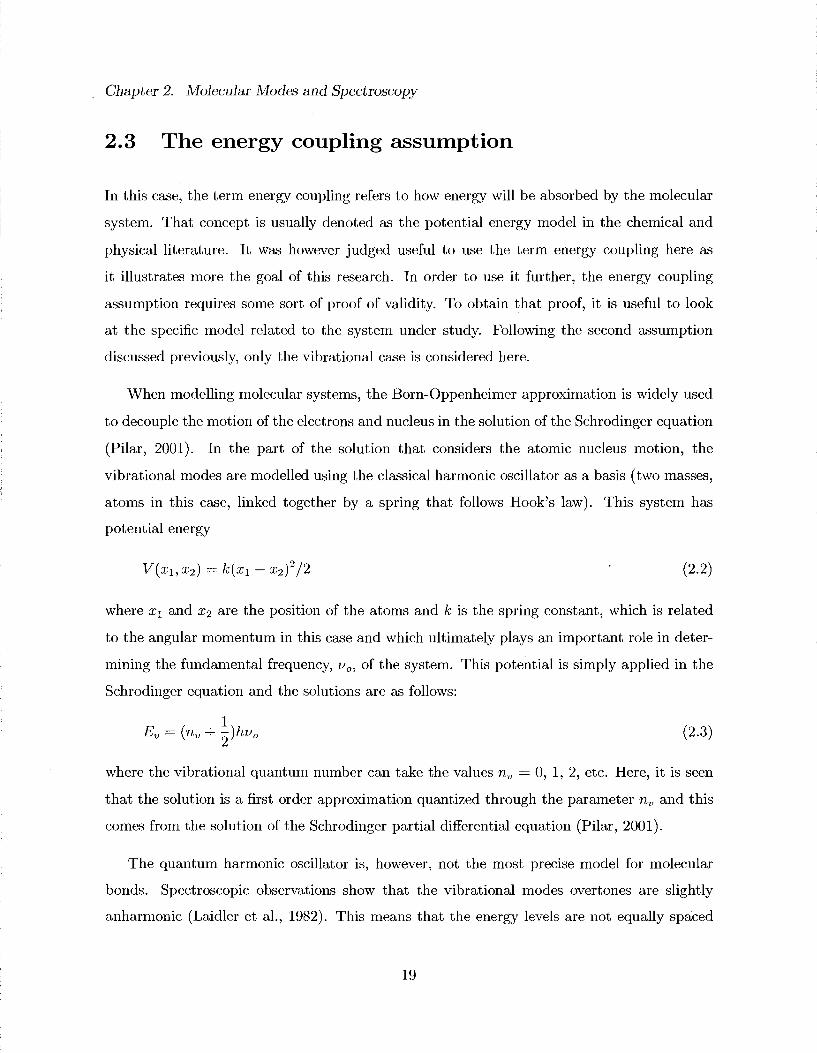
In the case of the more complex polyatomic molecules such as those of value for this study,
the same basic ideas apply. The most important difference arises from the multiplication
of posible vibrational modes. The general rule for determining the number of modes of a
molecule is as follows: given a molecule with n atoms, if it is a linear molecule, there are 3n — 5
vibrational modes, otherwise there are 3n — 6 vibrational modes. The additional modes are
due to the possible symmetric stretching, asymmetric stretching, bending, wagging, rocking
and twisting in all planes of the individual bonds or groups, as shown on figure 2.3 for the case
of H 2 0 (Laidler et al., 1982). Note that phenomena such as anharmonicity are also present
in this case.
24

Chapter 2. Molecular Modes and Spectroscopy
Electronic modes refer to the regions where electrons are located around an atomic nucleus.
Such regions are the zones where there is a non negligible probability of having an electron
present. The probabilities are computed using the wavefunction through solutions of the
Schrodinger equation (Levine, 2005). The atomic system is often modelled as a finite potential
well and the solutions for a single dimension are standing waves which integrally fit the
"radius" of the orbit (note that these solutions are fully compatible with the energy coupling
assumption). This wave-like behaviour is at the base of the famous wave-particle duality and
was first proposed by DeBroglie (Pilar, 2001).
As discussed before, the energy function of an atomic bond usually has the form of the well
known Morse potential. The curve shown on figure 2.1 represents a single electronic state.
The different possible energies on the curve are quantized and these states are the different
rotational and vibrational modes of the given electronic mode (Pilar, 2001). Hence a change
in electronic state is represented as a jump to another curve of very similar shape with higher
or lower energy. It can thus be seen that the absorption of an energy photon below a certain
limit will increase the energy of the molecule through rotational and/or vibrational modes.
Beyond the limit, an electronic transition (to another potential curve) will take place .or the
bond will break. Such an electronic transition can be accompanied or not by a rotational-
vibrational transition. The determination of the final rotational-vibrational state during the
electronic transition is made using the Frank-Condon principle which states that the overlap
of the wave-functions of the initial and final state must be maximized (Levine, 2005).
Most electronic transitions starting from the ground state occur in the visible and ultravi
olet part of the spectrum (wavelengths below 700 nm). This frequency range is scanned by a
UV-visible spectrophotometer and the peaks observed can be linked to electronic transitions
(Pavia et al., 2001). This particular data is important here as it sets a limit of validity due to
the assumption requiring only vibrational dissociation. Therefore, the highest wavelength at
which an electronic transition peak is located should be regarded as the smallest wavelength
to consider when applying the energy coupling assumption.
It is now clearer how the global spectrum of energetic molecules should be studied in
25

Chapter 2. Molecular Modes and Spectroscopy
order to perform the required calculations. The infrared spectrum contains the fundamental
vibrational information of the ground electronic state of a molecule and the rotational modes
are embedded in that spectrum as well (although often not discernable because of the precision
required). The first electronic transitions are usually found in the higher energy part of the
spectrum (often in the wavelengths around 200 nm) (McHale, 1999). This sets a limit on the
multiple of the base vibrational frequencies that can be applied to get dissociation. Beyond
this limit, the dissociation energy and the vibrational spectrum of the new electronic state (or
Morse potential curve) will be required. The scope of this study is however to remain in the
ground electronic state.
2.5 Molecular dissociation
The most important phenomenon studied in this work is molecular dissociation. The ways in
which a bond can break are exposed here with respect to the previous discussions. Molecular
dissociation occurs through vibrational or electronic excitation. When the vibrational energy
of the bond is such that the rightmost part of the Morse potential curve is reached, the
bond will break. The difference between the ground vibrational energy and the asymptotic
value of the energy in a Morse potential function is defined as the dissociation energy on
that given electronic level (or Morse curve) (Pilar, 2001). The dissociation energies values
found in the literature all refer to the ground electronic state and are often obtained using
spectroscopic measurements (as a difference between the excited species dissociation fragments
excess energy and the electronic transition energy) (Barrow, 1966). It is important to note that
the dissociation energies found in the literature usually only refer to the two direct members
of the bond (for exemple a C-C bond alone that is not part of a larger molecule). In a
larger molecule, the mechanics and forces of the system shall cause variations in these values.
Hence, the use of literature dissociation energies here must be viewed as a simplification.
In the case of dissociation through electronic excitation, an electron that receives a photon
with energy large enough to escape the potential well or raise the electron to an antibonding
orbital can cause the bond to break (Levine, 2005). The combination of both a vibrational
26

Chapter 2. Molecular Modes and Spectroscopy
and an electronic transition can cause dissociation. The reason for such behaviour is found
directly in the Prank-Condon principle. By this statement, it is well possible that in order
for the wavefunctions of the initial and final states to have the maximum overlap, the final
state will be in a different vibrational mode (McHale, 1999). The energy of the system could
however be located on the asymptotic part of the new Morse curve and cause dissociation.
Hence, although the dissociation is caused by the vibrational energy, the electronic transition
is causing the shift to a vibrational mode where bond breaking becomes possible (Laidler et
al., 1982). Again, it must be stressed that this study is confined to the case of dissociation
through the sole vibrational excitation.
2.6 Summary
This chapter has laid the theoretical foundations on which the method is built. It is noted
that the present study looks only at molecular dissociation due to the excitation of vibrational
modes. The main assumption has been shown to be the energy coupling statement. The
application of the energy coupling assumption has two major implications. The first one is of
a more qualitative nature as it answers the question of how incoming energy will interact with
the molecular system. The second implication is more quantitative and enables one to calculate
the overtones of the fundamental vibrational frequency all the way to the dissociation limit.
One must note that this last implication is dependant on the model used for the potential
energy (the quantum harmonic oscillator and the Morse potential were looked at in this case).
The choice of the quantum harmonic oscillator model here was purely based on the realisation
that the added complexity of using the Morse potential in the calculations was not warranted
by the slight increase in the precision of the final results. One must however note that if
intermediate overtones are to be considered (the frequencies between the fundamental and
the dissociation), the simple quantum harmonic oscillator should not be used as it will not
be precise enough (an example would be the calculation of the vibrational partition function
of a bond). The other assumptions are also important to the method but remain more
straightforward.
27

Chapter 2. Molecular Modes and Spectroscopy
It is useful to conclude this chapter by explicitly giving the steps required to apply the
method developed. Upon reviewing the different steps, the importance of the assumptions
used is easily seen. The method is given here in a list form:
1. Obtain the infrared and ultraviolet spectra information of the energetic molecule to be
studied (this information can either be graphical or tabular peaks values)
2. Prom the knowledge of the different molecular bonds present (for example through a
drawing of the molecule), use the literature data to assign bands wavelengths regions
to specific bonds (textbooks on infrared spectroscopy usually contain numerous tables
with such assignments).
3. Compare the data of steps 1 and 2 to assign absorption peaks to specific bonds.
4. Using literature values of the dissociation energies, the Planck's law is applied directly
to find the exact dissociation frequencies (or wavelengths).
5. From the results of the two previous steps, calculate the exact quantum number value
(not necessarily an integer) that will yield the dissociation frequency. Note that the
quantum number value obtained should be rounded up to the next integer value to yield
a result consistent with the energy coupling assumption in this case.
6. Calculate the frequency that matches the rounded value obtained in the last step. This
frequency is the limit below which there will be no dissociation. A table of frequencies
with respect to the quantum number can also be produced to show the progression of
the overtones from the fundamentals to the dissociation limits.
Thus, it can be seen that the results of these calculation are data tables with fundamental
and dissociation parameters (energies, frequencies, wavelengths, and quantum numbers). Each
fundamental frequency in a table is linked with an actual mode directly in order to be able
to further the analysis and predict which bond is subject to break first in a given case. The
next chapter will apply the method presented here to the case of two widely used energetic
molecules.
28

Chapter 3
Application of the Method
3.1 General overview
The last chapter presented the proposed method to study the initial condensed phase com
bustion reaction and established some basic ground rules to examine spectra of molecules in
order to better predict the dissociation phenomena. In this chapter, the method and rules are
applied to the cases of the following energetic materials: nitroguanidine (NQ) and nitrocel
lulose (NC). The choice of these particular molecules is not arbitrary as they are not in the
same family (a nitramine and a nitrate ester). In both cases, the analysis shall follow the same
path with these given steps: infrared spectrum analysis, ultraviolet-visible spectrum analysis,
applying the assumptions to calculate the limit wavelengths, and discussion on the results.
3.2 Example: Nitroguanidine
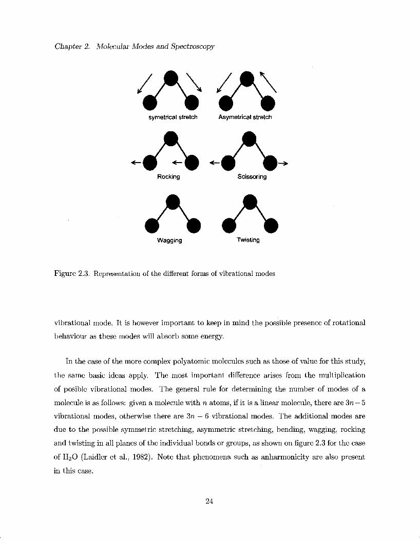
The vibrational modes of NQ can be obtained from the infrared spectrum on figure 3.1 (Sigma
Aldrich catalog). The NQ spectrum shows several bands (or peaks) of absorption. It was
shown that each band is centered at the vibrational mode frequency and that the thickness of
the band is due to the rotational fine structure. It can be observed that more precision would
29
Chapter 3. Application of the Method
s / • " " ,
'fV 1"
.....
I
/ A 1
v\
r\
\
i i
/ ,,-, f
\
• i i 1 * 1 V
A^1' ^ 1 '"
—
^ i
-'.... 1/A
nnj . .../I.. t / \ \ / \.
1
0^_J , , ••• . ! L i ! i , L I . . .1 - J 1 ^ i . .. . _ i - J ' * 41)09 380O 3600 WOO 3200 5000 2860 2600 ! W 2200 2000 1800 1600 14D0 1200 lOOO 800 800 450
WAVEKUMBenS
Figure 3.1. The infraxed spectrum of nitroguanidine (Sigma Aldrich Catalog)
be required to show the detailed structure here. From figure 3.1, three separate zones can
be noticed: one around 1500 cm - 1 , one around 2900 cm - 1 , and one last around 3300 cm - 1 .
It is not enough here to simply note the presence of a particular band. The peaks must be
assigned to specific bonds in order for conclusions to be drawn from the calculation. This is
done by consulting infrared spectroscopy group frequencies tables found in the literature. It
is required here to be able to assign each band to a particular group bond in order to perform
the dissociation calculation which comes after. When comparing a spectrum plot with actual
individual bond data, it is important to keep in mind that there will be slight shifts in the
frequencies due to the nature of what is attached on either side of the group which affects the
mechanics of the oscillations (Mayo et al., 2004).
The nitroguanidine (NQ) molecule is shown on figure 3.2. This molecule contains elements
of an aliphatic amine (R-NH2) and an aliphatic nitrate (R-NO2) together. The detailed
spectroscopic data is presented as follows in a list form:
• The asymmetric and symmetric stretches of NH2 are 3375 + / - 25 c m - 1 and 3300 + / -
30 cm - 1 , respectively (Pavia et al., 2001).
• The scissoring and wagging frequencies of NH2 are respectively at 1620 + / - 30 c m - 1
30

Chapter 3. Application of the Method
H
N — H
H N C
N
H
Figure 3.2. Schematic of the nitroguanidine molecule
and 800 cm"1 (Mayo et al., 2004).
• The N-H stretches are around 3400 cm"1 (Pavia et al., 2001).
• The C-N stretch is at 1665 + / - 25 cm"1 (Mayo et al., 2004).
• The asymmetric and symmetric stretches of NO2 are 1531-1601 cm"1 and 1310-1381
cm"1, respectively (Mayo et al., 2004).
• The in-plane bending, out-of-plane wagging and in-plane rocking frequencies of NO2 are
610-660 cm"1, 477-560 cm"1 and 470-495 cm"1, respectively (Mayo et al., 2004).
• There are two close together bands around 2900 cm"1. Literature shows clearly that
such bands are usually the first to look for in an organic compound as they are the C-H
stretching modes. NQ, however, does not contain any C-H bond. The hypothesis here
is that the NQ could be in some organic solvent (Pavia et al., 2001). Hence these bands
should be neglected in the analysis.
N
O
31

Chapter 3. Application of the Method
This covers most of the bands seen on figure 3.1. Note that given the location of the two
band zones, overtones are normally expected to occur around 3000 c m - 1 and 6000 cm - 1 . Since
overtones are of weaker intensities, they are not always observed and can be hidden by other
bands. Hence some bands such as those in the higher frequency region (2500-3500 cm - 1 ) can
be mixed with overtones. However this is not expected to modify the observation made above
as the actual modes are stronger then the overtones. Two standalone bands that have not
been discussed yet (around 1100 cm"1) could indeed be overtones as well. The only question
in this case is if the NQ sample was in another organic substance (such as a solvent) that
could have created the two 2900 cm"1 bands. If so, then some of the not directly explained
bands could also be possibly coming from this same substance.
The UV spectrum of NQ, given on figure 3.3, shows the electronic transitions frequencies
(National Institute of Standards and Technologies). It is seen that there are two wavelengths
(frequencies) of interest in this case (corresponding to maxima in the spectrum): 210 and 260
nm. Hence any wavelength close to or below these last two values should not be used to make
any conclusion.
Based on the data presented previously, the dissociation wavelength can be computed
using the method presented in chapter 2. The results of the dissociation calculations for NQ
along with a compact list of the IR modes are shown on table 3.1. Note that the wavenumber
values given are the central band values (maxima) on the actual spectrum of NQ and that the
dissociation energies are from the literature (Franklin and Marshall College). It can be seen
that the matching n values (frequency multiple to reach dissociation energy) are not integers.
Since the permitted values of n are integers here, the first actual dissociation n values are
the rounded up integer values. The set of possible wavelength between the fundamental
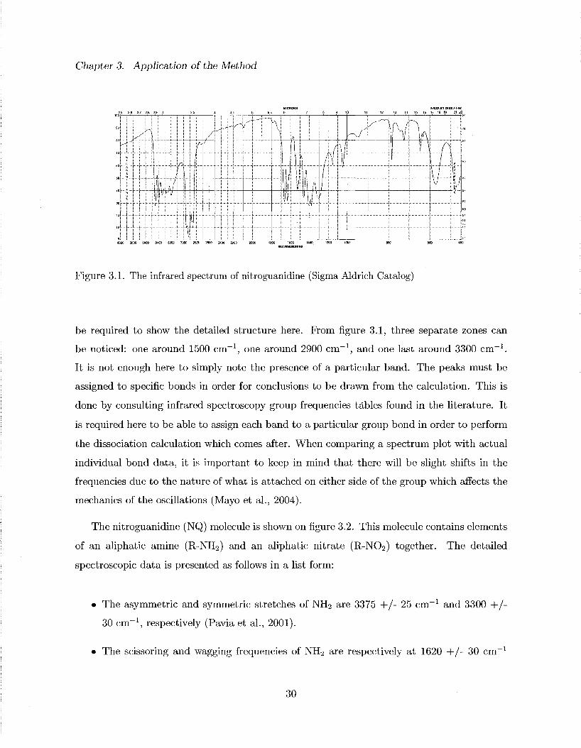
and dissociation values have been tabulated and are shown in Appendix A. A graphical
representation of this tabular data is shown on figure 3.4. Note that figure 3.4 is only an
illustration of what would be observed and has not been generated by any calculations. The
intermediate frequencies shown in figure 3.4 are coming from the use of both the quantum
harmonic oscillator and the Morse potential.
32

Chapter 3. Application of the Method
Logarithm epsilon
4.0 h
Guanidine, niiro-
W M 8 SPECTRUM
3,6
3.2
2.8
vvaveleridlh (nm)
Figure 3.3. The ultraviolet spectrum of nitroguanidine
As an example, the full detailed calculation performed for the single bond N 0 2 symetric
stretch is shown below. Note that the step numbers used are the same as those presented at
the end of chapter 2.
1. The IR and UV-visible spectra are shown on figures 3.1 and 3.3.
2. The assignment of band wavelength region is given in list format.
3. The assignment of absorption peaks to specific bond is shown on table 3.1. In the case
of the NO2 symetric stretch, the assigned wavenumber is 1300 cm - 1 .
4. The dissociation energy for an N-0 single bond can be found to be 2.3 eV. Using Planck's
law (E = hu), the following is obtained: u = E/h. Substituting for the energy value
33

Chapter 3. Application of the Method
Mode description
NH2 asyin stretch
NH2 sym stretch
NH2 wagging
NH2 scissoring
NH stretch
C=N stretch
C-N stretch (NH2)
C-N stretch (N()2)
NO2 sym stretch (N-O)
NO2 sym stretch (N=0)
NO2 asyin stretch (N-O)
NO2 asyin stretch (N=0)
NO2 rocking (in)
NO2 wagging (out)
NO2 bending (in)
N-N bond
wavenumber
(1/cm)
3350
3270
780
1630
3450
1660
1050
1160
1300
1300
1530
1530
480
570
650
NA
bond il/
(oV)
4.01
4.01
4.01
4.01
4.01
6.38
3.17
3.17
2.3
6.3
2.3
6.3
2.3
2.3
2.3
1.73
A (m)
3,0E-06
3.1E-06
1.3E-06
6.1E-06
2.9E-06
6.0E-06
9.5E-06
8.6E-06
7.7E-06
7.7E-06
6.5E-06
6.5E-06
2.1E-05
1.8E-05
1.5E-05
NA
frequency
(Hz)
1.0E+14
9.8E+13
2.3E+13
4.9E+13
1.0E+14
5.0E+13
3.2E+13
3.5E+13
3.9E+13
3.9E+13
4.6E+13
4.6E+13
1.4E+13
1.7E+13
2.0E+13
4.18E+14
nv
match
9.6
9.9
41.4
19.8
9.4
30.9
24.3
22.0
14.2
39.0
12.1
33.2
38.6
32.5
28.5
NA
nv
exact
10
10
42
20
10
41
25
23
15
40
13
34
39
33
.29
NA
limit A
(nm)
310
310
310
310
310
195
392
392
540
197
540
197
540
540
540
718
diss A
(nm)
299
306
305
307
290
194
381
375
513
192
503
192
534
532
531
NA
AA (nm)
11
4
4
3
20
0
11
17
27
5
37
5
6
8
9
NA
Table 3.1. Spectroscopy analysis and calculation results for nitroguanidine
given above and planck's constant in appropriate units (4.1 x 1CT15 eV s), the follow
ing frequency is obtained: u = 5.56 x 10¹⁴ Hz. This last frequency corresponds to a
wavelength of 540 nm (shown in table 3.1).
5. The fundamental frequency can be computed directly from the wavenumber value as
signed in step 3: v = c/X where A = 1/fc (here, k is the wavenumber). Using the velocity
of light constant of 3 x 10⁸ m/s , the value u = 3.9 x 10¹³ Hz is obtained. The exact
dissociation quantum number is thus the ratio of the dissociation and the fundamental
frequencies, which in this case yields 14.2. Hence the actual value of the first possible
dissociation quantum number is the rounded up integer nv = 15.
6. The first dissociation frequency value is then found from the following expression: Vdiss
= nv u0_ This yield Vdiss = 5.85 x 10¹⁴ Hz, which is equivalent to a wavelength of 513
nm (present in table 3.1).
It is interesting to compare the first dissociation wavelength of 513 nm with the limit value
34
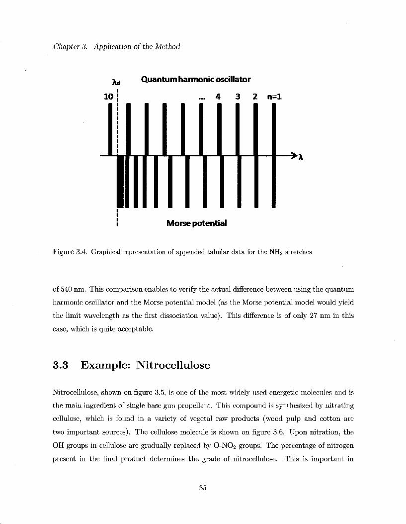
Chapter 3. Application of the Method
Ad
10
Quantum harmonic oscillator
... 4 3 2 n=l
* \
Morse potential
Figure 3.4. Graphical representation of appended tabular data for the NH2 stretches
of 540 nm. This comparison enables to verify the actual difference between using the quantum
harmonic oscillator and the Morse potential model (as the Morse potential model would yield
the limit wavelength as the first dissociation value). This difference is of only 27 nm in this
case, which is quite acceptable.
3.3 Example: Nitrocellulose
Nitrocellulose, shown on figure 3.5, is one of the most widely used energetic molecules and is
the main ingredient of single base gun propellant. This compound is synthesized by nitrating
cellulose, which is found in a variety of vegetal raw products (wood pulp and cotton are
two important sources). The cellulose molecule is shown on figure 3.6. Upon nitration, the
OH groups in cellulose are gradually replaced by O-NO2 groups. The percentage of nitrogen
present in the final product determines the grade of nitrocellulose. This is important in
35
Chapter 3. Application of the Method
H / /
/ /
H O N
H O O
— - -o • H o-—-
H H O
H N
H
O
Figure 3.5. Schematic of the nitrocellulose molecule
applications as it has an impact on the energetic potential of the NC used. In the present
case, the impact will be that OH group bands are to be expected depending on the grade of
the NC represented in the infrared spectrum. It is important to note that NC consists of long
chains of the cyclic group shown on figure 3.5 and connected through the lateral oxygen atom
(two of these groups are represented on figure 3.5) (Akhavan, 1998).
The infrared spectrum peaks of nitrocellulose are given on table 3.2 and shown graphically
in Append ix B (Giasson, 2005). Three main features can be observed in this spectrum: two
standalone bands are present around 3000 cm - 1 , the majority of the band are in the 1000-1500
c m - 1 region and several scattered bands are seen under 1000 cm - 1 . A literature review on
the different groups and bonds present in the NC molecule yields the following information:
The asymmetric and symmetric stretches of NO2 are 1620-1640 cm l and 1270-1285
36
Chapter 3. Application of the Method
H
H _ c _ _ _ 0 _ _ _ H
H — — C — O
/ \
/ \ / H C C H
H
Figure 3.6. Schematic of the cellulose molecule
cm - 1 , respectively (Mayo et al., 2004).
• The N-0 stretch is in the interval 855-870 cm"1 (Mayo et al., 2004).
• The C-H stretch is located around 2700-3100 cm"1 (Pavia et a l , 2001).
• The C-0 stretch is located in the interval 1000-1300 cm"1 (Pavia et al., 2001).
• The in-plane bending and out-of-plane wagging are located in the intervals 755-760 c m - 1
and 695-710 cm"1, respectively (Pavia et al., 2001).
• The C-C bond stretches are very weak and will often mechanically couple. Hence, these
cannot easily be observed and/or assigned.
All the modes described above have strong absorption and can easily be observed on the
spectrum of table 3.2 (or in Appendix B). The detailed assignments are shown on table 3.3.
37

Chapter 3. Application of the Method
693 cm 751 cm 841 cm 1004 cm
1071 cm - 1 1162 cm - 1 1279 cm - 1 1377 cm
1428 cm - 1 1652 cm - 1 2916 cm - 1 3573 cm
Table 3.2. FT-IR spectroscopy peaks wavenumbers values
Mode description
0-H bond stretch
C-H bond stretch
C-0 bond stretch
C-C bond stretch
N-O bond stretch
NO2 sym stretch (N-O)
NO2 sym stretch (N= 0 )
NO2 asym stretch (N-O)
NO2 asym stretch (N=
NO2 bending (in)
NO2 wagging (out)
=0)
wavenumber
(l/cm)
3573
2916
1071
weak
841
1279
1279
1652
1652
751
693
bond E
(eV)
4.76
4.26
3.71
3.59
2.3
2.3
6.3
2.3
6.3
2.3
2.3
A (m)
2.8E-06
3.4E-06
9.3E-06
NA
1.2E-05
7.8E-06
7.8E-06
6.1E-06
6.1E-06
1.3E-05
1.4E-05
frequency
(Hz)
1.1E+14
8.7E+13
3.2E+13
NA
2.5E+13
3.8E+13
3.8E+13
5.0E+13
5.0E+13
2.3E+13
2.1E+13
n„ match
10.7
11.8
27.9
NA
22.02
14.5
39.7
11.2
30.7
24.7
26.7
nv
exact
11.0
12.0
28.0
NA
23.0
15.0
40.0
12.0
31.0
25.0
27.0
limit A
(nm)
261
292
335
346
540
540
197
540
197
540
540
diss A
(nm)
254
286
333
NA
517
521
195
504
195
533
534
AA (nm)
6
6
1
NA
23
19
2
36
2
7
6
Table 3.3. Spectroscopy analysis and calculation results for nitrocellulose
It was not possible to obtain the ultraviolet-visible spectrum of NC in a graphical format.
A study by Gavrilov and Ermolenko published in 1967 was found where the main absorption
values were given in the UV-visible spectrum of cellulose and cellulose derivatives (including
nitrocellulose). From this study, it is clear that an absorption peak is present in the region
around 200-240 nm for NC (Gavrilov et a!., 1967). Hence, the limiting wavelength of validity
should be taken as 240 nm in this case.
The full calculation results are shown on table 3.3. Note that that steps used here are
exactly the same as those needed for nitroguanidine, hence a sample calculation is not required
here. Note here that the difference between the limiting wavelength and the first dissociation
value is again quite acceptable. Again the intermediate frequencies are tabulated in Appendix
A.
38
Chapter 3. Application of the Method
Nitroguanidine dissociation wavelengths (nm)
100 aoo BOO 400 50b 600 700 BOO
Nitrocellulose dissociation wavelengths (nm)
Figure 3.7. First dissociation wavelengths calculated for NQ and NC
3.4 Discussion on the calculations results
Interesting similarities arising from the presence of similar groups can be observed for both
the nitrocellulose and the nitroguanidine case. Figure 3.7 shows a graphical representation
of all the first dissociation wavelengths for both cases (the blue lines refer to NQ and the
red lines to NC). The small differences that are observed between values of a same group
arise from the differences in the fundamental frequencies. Thus those differences are caused
by the different nature and geometry of each molecule. Another important fact to realize is
that only small differences are observed between the dissociation wavelength calculated from
both potential model (quantum harmonic oscillator and Morse potential). This would tend
to show that going through the full spectral analysis is not warranted to attain the goals of
this work. However, showing the smallness of this difference is important at this stage and
39

Chapter 3. Application of the Method
the failure to do so would have shown a lack of completeness. Furthermore, any continuation
to this work leaning toward computing other combustion properties will require performing
statistical mechanical calculations. Such calculations shall require the partition function to
be known, thus requiring the fundamental modes to be known. Therefore for these reasons,
it is necessary to go through the spectroscopic analysis step.
The main conclusion to make concerning these calculations is that the nitrate group (or
NO2 group) is the one that requires the minimum amount of energy to break and thus that
would be most prone to begin a combustion reaction. However, to state that a group or
another shall begin the reaction, the spectrum of the excitation energy must be examined as
the quantum nature of the system will require very specific energy values in order to excite
very specific bonds (or groups). The comparison of the results obtained in this chapter and
the input energy spectra is the main subject of the following and last chapter of this thesis.
40

Chapter 4
Energy Input Spectrum and Ignition
4.1 General overview
The last two chapters focused on validating and showing how to use a simplified method
that enables one to predict how input energy will couple to a given molecular bond and if
dissociation is likely to occur. However, to be useful in practical applications, one additional
step must be performed: comparing the spectrum of possible excitations with the spectrum
of the incoming energy to find out if there are any matches. This last task is not as simple as
it could seem as the source of this energy cannot be neglected in the evaluation. The subject
of ignition thus becomes of importance in order to better characterize each type of source
and apply the method developed in this work accordingly. This last chapter will first address
this issue of ignition along with giving a list of possible energy sources. One such sources
shall then be expanded on by using published emission spectroscopy data and the calculation
examples of chapter 3 (nitroguanidine and nitrocellulose). A discussion follows on application
with other input sources focusing on future research that could ensue from this work.
41

Chapter 4. Energy Input Spectrum and Ignition
4.2 Ignition and some possible sources
Ignition is usually denned as the onset of the self-sustained reaction that is combustion (Meyer,
2003). Hence, the activation energy required to break the first bonds is exactly the ignition
energy. Ignition has been described in most publications as mostly a thermal problem by
opposition to a photodissociation issue (De Young, 1995; Babrauskas, 2003). However, the
term "thermal", although pointing to the concepts of heat transfer and ignition temperature,
is not a very precise one. In present modelling, the classical heat transfer theory is applied
to simulate the temperature rise to the ignition temperature where the combustion chemistry
is added into the analysis (Beckstead, 2006). It is however interesting to note that concepts
such as temperature and heat transfer actually represent deeper molecular issues.
• Temperature is recognised as the measure of the total energy contained in the molecular
system, which generally consists of the translational, rotational and vibrational energies
(Hill, 1987).
• Heat transfer has three modes; conduction, convection and radiation. Conduction di
rectly involves the spreading of vibrational motion through a solid substance. Radiation
consists of transfer through electromagnetic energy, or photons (Holman, 2001).
Thus it is seen that although the term thermal is used, there is a deeper implication with
the molecular structure and dynamics that has been covered all through this study. Prom
the above considerations, ignition can thus be more precisely described as an excitation of
certain molecular vibrational, translational or electronic modes causing the rupture of their
corresponding bonds. It is then natural to realize that understanding a given energy input
mechanism becomes important in the analysis. Several such mechanism relevant to propellant
combustion are listed here:
• Temperature: In this case, the temperature is viewed as the sole source of molecular
excitation. In the case of solids, only vibrational modes are involved. It is important
42
Chapter 4. Energy Input Spectrum and Ignition
in this case to well understand phenomena involved in changing the temperature of
a sample (interactions). The simplest case would be to consider different steady state
temperatures without any external stimulus that would cause variation. Such a problem
is beyond the scope of this work but would be an interesting continuation.
• Photodissociation: This simple case considers a photon being absorbed by a given bond
that would excite the bond to a dissociation vibrational energy level. It is obvious to
observe that this case can be easily applied to the method developed in this research.
This last case presented shall be the one expanded in this chapter. In order to obtain
the correct input energy spectrum, more must be known about the source itself. In the case
of propellant combustion, this source is most often either the combustion of an initiating
compound (such as the well known black powder) or the combustion of the propellant itself
(in a chain reaction where part of the energy liberated by the decomposition of the material
goes back into providing the activation energy to more of the material). The first source thus
usually governs the beginning of the combustion and the second will guide what remains. The
next section will look at these different sources through some examples.
4.3 Input spectrum through emission spectroscopy
The spectroscopic data collected from analyzing the light emitted during combustion is usually
referred to as an emission spectrum (as opposed to the absorption spectra that were reviewed
before). Emission spectra are usually studied to determine the combustion products during a
given reaction as different radicals will exhibit certain frequency bands only. It thus becomes
interesting to compare the dissociation wavelengths of a given energetic molecule and the
emission spectrum of any of the substance present in the combustion. As stated previously,
in this case the two substances likely to be present will be the igniter composition (such as
black powder) and the main energetic molecule. For one to predict the initial reaction, it then
becomes a matter of determining by inspection which ignition wavelengths are embedded in
emission regions.
43

Chapter 4. Energy Input Spectrum and Ignition
Emission intensity
200 nm 400 nm 600 nm
Figure 4.1. Comparison of dissociation wavelengths of NC with the emission spectrum for JA2
As an example, emission spectra in the visible-UV region of propellants containing in
gredients discussed in chapter 3 can be studied. For the purpose of this work, the emission
spectrum of JA2 propellant is a good first example. The energetic ingredients contained in
JA2 are the nitrate esters nitrocellulose, nitroglycerin, and diethylene glycol dinitrate. The
emission spectrum curve of JA2 begins rising from an intensity of zero at about 375 nm and
has a fairly linear rise (Eisenreich et al., 2000). Plotting this with the nitrocellulose dissocia
tion wavelengths (by drawing vertical bars at bond breaking values) enables the comparison
leading to a prediction to be made (see figure 4.1). Observing figure 4.1 enables one to quickly
determine that the NO2 groups of the NC molecule shall be the first to secede as they are
the only with dissociation wavelengths high enough to be in the region of emission. Upon
absorption of the photonic emission of burning JA2 propellant, NC (as shown in figure 3.5
with the main cycle shown having x repetitions) will initially decompose as follows according
to the model developed in this work:
NC (C 6H 8N 20 9) x= (C 6 H 8 0 5 ) x + (2N02)x (R-7)
It is interesting to look at other combustion emission spectra from other energetic materials
44
OH CO&CC
NO2 I CH
J A2 Flame emissions curve
NO2
NCfe^
_ ^ . 1

Chapter 4. Energy Input Spectrum and Ignition
Emission intensity NO2&CN
NH2
200 nm
General flame emissions curve
CN
NO2
400 nm 600 nm
NN
* X
Figure 4.2. Comparison of dissociation wavelengths of NQ with the general emission spectrum trend
as some similarities can be observed. More precisely, the emission spectra from an RDX pro-
pellant (Weiser et al., 1999) and pyrotechnic compositions (Gillard et al., 2002) were studied.
The quasi-linear increase from a zero intensity starting at wavelengths in the range 350-450
nm can quite often be observed. This seems to indicate that emissions in the ultraviolet range
are not common in combustion phenomena. Hence the first reaction derived for NC can be
reasonably expected not to change. Furthermore if the same analysis is applied to NQ, the
initial reaction derived is the following:
CH4N402(nitroguanidine)=HCN + NH2 + NH + N0 2 (R-8)
It can be noted that this last reaction is exactly the same as reaction R-2 given in the first
chapter when discussing the condensed phase reactions of energetic molecules families. The
graphical representation of the analysis for NQ is shown on figure 4.2.
The application of the results obtained in the method developed in this work to combustion
emission spectroscopy has shown here to yield results that are aligned with the current ideas
about initial reactions for the case of nitrocellulose and nitroguanidine (a nitrate ester and a
nitramine with different groups). This was however a very simple way to rapidly apply the
45

Chapter 4. Energy Input Spectrum and Ignition
results in order to get meaningful information. It is obvious that other sources must also be
studied for completeness. The following section introduces another such source along with
some intricacies brought about by considering this source.
4.4 Ignition through a temperature rise
Certain points must however be put forward in order to better analyze the present case.
Prom the observation of the spectroscopic analysis results, it can be noticed that the limit
wavelengths are all in the visible and ultraviolet range (i.e. in the range between 200 nm and
700 nm). Since these wavelengths are within the range of ambient light, it can be concluded
that these dissociation reactions should be occurring constantly under normal conditions.
This is indeed the case and that situation is a major product safety concern for propellant
designers (short and long term propellant stability) (Urbanski, 1984). In the case of widely
used energetic substances, these decomposition reactions are occurring at a fairly slow rate but
the decomposition products increase the acidity of the surroundings which gradually causes
an augmentation of the reaction rate. Because of this feedback effect, the substance can reach
a state where the reaction rate will jump up and a fast combustion will occur. This jumping
point that separates the regime in which the material exists in a relatively stable form and
that in which a violent reaction occurs is of course what is normally referred to as the ignition
point (Kubota, 2007). From a statistical mechanics standpoint, there should be an important
increase of the number of bonds with an energy equal or grater then what is required for
dissociation at the point of ignition. It is interesting to realize that the phenomenon is merely
a rate increase of something that is already occurring. Hence the conclusion is that ignition
has to do with the kinetics of the process. Kinetics is, however, beyond the scope of the
present work but should be viewed as a necessary step in order to examine other sources, such
as temperature, in detail.
In the case of a solid, temperature is a measure of the total vibrational energy contained in
the system (Hill, 1987). Through statistical mechanics, the distribution of vibrational energy
46

Chapter 4. Energy Input Spectrum and Ignition
x U l
f
s w
it
•o c o
-O M -
o c 0 "C U ID ! •
u.
5.00E -05
4.00E -05
3.00E -05
2.00E -05
1.00E -05
0.00E+00
1500 1700 1900 2100 2300 2500 2700 2900
Temperature (K)
Figure 4.3. Fraction of bonds with the dissociation energy (NO2 stretches case)
levels can be calculated. The general expression used to calculate the percentage of units at
a given state with temperature is the following:
p-Ed/kbT
f(T) = (4.1)
where Z is the famous partition function (or sum-over-all-states function) and is denned as
follows:
Z = J2e-En/kbT
n=0
(4.2)
In order to correctly evaluate Z, the values of energies must be known as precisely as
possible (Hill, 1987). A correct model is required for this task. As discussed in chapter 2,
there are several such models available but the Morse potential function is more precise than
the quantum harmonic oscillator used for the method developed here. Hence the partition
function should be calculated with energy values obtained from applying the Morse expression
47

Chapter 4. Energy Input Spectrum and Ignition
(Laidler, 1982). Using the simple quantum harmonic oscillator model, the following partition
function is obtained:
e-hv0/2kbT
Applying this function to the percentage of units expression yields the distributions shown
on figure 4.3. The kinetic behaviour that is responsible for ignition can be observed on
figure 4.3 as an abrupt increase in the number units with sufficient energy for dissociation.
With an appropriate choice of the temperature value where the change of slope occurs, one
can determine a possible ignition temperature for the given case. However, the temperature
values that would be obtained with the case shown on figure 4.3 (around 2000 K) are not
at all close to known experimental ignition temperatures values (usually closer to 500-600 K
for typical energetic materials used for propellants). Hence, the model does not yield good
results as expected and the more precise Morse potential should be applied. This opens a new
direction and should be a direct next step in this line of research.
48

Chapter 5
Conlusions
5.1 Concluding remarks
From the results obtained in the different calculations and comparison made in this study,
the original assumption and ideas leading to the methodology chosen have been validated as
they corroborate well with the current ideas found in the literature. An important part of this
study was to perform a large literature review to assemble the different main ideas relevant
to condensed phase combustion and gasification combustion reactions. The elaboration and
proof of the different steps in the method along with the spectroscopic analysis of the two
examples has enabled to gather important information that will be useful in continuing this
research. That last achievement was an important goal of the present work as it was known
prior to the beginning that it would be an introduction to this type of simplified reasoning
applied to condensed phase combustion.
The main question that was invoked in the introduction was about the correct coupling
of energy with molecular systems. This question was answered mainly through the use of
potential energy models but the choice of model was shown to be dependant on the context
of the problem (Laidler, 1982). More precisely, the general method yielding dissociation
wavelengths was shown to be of acceptable precision with the simple quantum harmonic
49
Chapter 5. Conlusions
oscillator while any calculation requiring intermediate frequencies needs a more precise model
(such as the Morse potential). In addition, molecular systems in their ground electronic states
were assumed throughout the calculations as a first simplification.
The application of the method with the assumption of bond breaking solely through pho-
todissociation using emission spectroscopy has yielded results quite in agreement with current
theories regarding initial gasification reactions. The initial reactions for both nitroguanidine
and nitrocellulose were given explicitly. It is however obvious that temperature has an im
portant role to play in the later stage of the reaction but the assumption of photodissociation
seems reasonable at the early stage studied here. An important task to perform will be to
gather more emission spectroscopy data for the common cases (black powder ignition, stan
dard propellant, energetic molecules) to verify that there are no anomalies. This last task
coupled with applying the method with more molecules from different families will help in
ensuring that the method is generally valid. The ultimate engineering goal would be to find
an ingredient that would have photonic combustion emissions differing from those observed
in this study in order to modify the initial reaction in a precise fashion (and possibly modify
the propellant burning rate as well).
It was shown that there are many possible continuations to this research. The most obvious
is the application of statistical mechanics principles to accurately predict the run-up point of
the temperature distribution curve for different bonds and determine the ignition temperature.
This will be more complex due to the calculations involved but the spectroscopic data obtained
from the analysis shall be essential in performing the analysis. Another important sequel would
be to obtain the pyrolysis law parameters (see equation 1.1 in chapter 1) through calculations
using the principles introduced here. This again would involve statistical mechanics as kinetics
is involved in deriving a reaction rate law. There would also be other, more applied, studies
such as other ignition sources like laser, electric discharge, plasma, and shock interaction with
an energetic molecule.
Following the additional verifications discussed above, the method should be applied to
a current propellant burning rate prediction algorithm in order to have a complete tool that
50

Chapter 5. Conlusions
would not require a guessing step (Miller and Anderson, 2004). This is important as it was
through the review of literature pertaining to this subject that came the original idea for
pursuing the research done here. To conclude, the goals of defining a way in which the energy
couples to an energetic molecule, acquiring molecular modal data through spectroscopy, and
predicting an initial reaction to the combustion of a given energetic molecule were attained
with success. The first results obtained are in agreement with currently published ideas.
Hence, through gathering additional data to reinforce the conclusions and pursuing the re
search in the areas mentioned previously, the empirical methodology introduced here shall be
more completely validated. This will contribute in increasing our understanding in condensed
phase combustion and shall enable designers to successfully come up with new and efficient
applications.
5.2 Contribution to knowledge
Throughout the initial chapter of this thesis, it was stressed that current methods used to
study condensed phase combustion require very complex computations that render the whole
analysis expansive and inefficient. It was the main goal of this work to lay the foundations of a
simplified methodology through theoretical considerations and empirical measurements. These
measurements are mainly made through absorption and emission spectroscopy. Care was taken
in verifying the simplification steps and assumptions through basic quantum mechanics. The
two examples used showed that the methodology leads to predictions that are within the
current thoughts about gasification reactions. The tools gathered in this thesis can now be
readily applied with statistical mechanics in order to cover the kinetics aspect and thus have a
more complete picture of the condensed phase combustion phenomena. The results obtained
along with those already available from the conclusion of this work shall prove useful in
designing more complete combustion modeling tools.
51
References
[1] Akhavan, J. (1998) The Chemistry of Explosives. Royal Society of Chemistry.
[2] Allen, G. and Pritchard, H.O. (1974) Statistical Mechanics and Spectroscopy. Halsted.
[3] Babrauskas, V. (2003) Ignition Handbook. Fire Science Publishers.
[4] Barrow, G.M. (1966) Physical Chemistry. McGraw-Hill.
[5] Beckstead, M. W. (2006) Recent progress in modeling solid propellant combustion. Combust, Expl. Shock Waves 42 (6), pp. 623-641.
[6] Beyer, R.A. and Pesce-Rodriguez, R.A. (2004) The response of propellants to plasma radiation. Proc. 12th symposium on Electromagnetic Launch Technologies.
[7] De Yong, L., Nguyen, T. and Waschl, J. (1995) Laser ignition of explosives, pyrotechnics and propellants: A review, DSTO Internal Report, DSTO-TR-0068.
[8] Dlott, D.D. (2003) Fast molecular processes in energetic materials. Theoretical and Computational Chemistry; Energetic Materials - Part 2: Detonation and Combustion, pp. 125-192.
[9] Eisenreich, N., Eckl, W., Fisher, T., Weiser, V., Kelzenberg, S., Langer, G. and Baier, A. (2000) Burning phenomena of the gun propellant JA2. Propellants, Explosives and Pyrotechnics 25, pp. 143-148.
[10] Franklin and Marshall College, Lancaster, PA. website: http://wulfenite.fandm.edu.
[11] Gavrilov, M.Z. and Ermolenko, I.N. (1967) Electronic absorption spectra of some cellulose derivatives. Zhumal Prikladnoi Spektroskopii 6 (6), pp. 754-758.
[12] Giasson, G. (2005) FT-IR measurement curve on nitrocellulose. Technical Report, General Dynamics - Ordinance and Tactical systems Canada - Valleyfield.
[13] Gillard, P., De Izarra, C. and Roux, M. (2002) Study of the radiation emitted during the combustion of pyrotechnics charges. Part II: characterization by fast visualization and spectroscopic measurements. Propellants, Explosives and Pyrotechnics 27, pp. 80-87.
52

[14] Hill, T.L. (1987) An Introduction to Statistical Thermodynamics. Dover Publications.
[15] Holman, J.P. (2001) Heat Transfer. 9th edition, McGraw Hill.
[16] Kee, R.J., Grear, J.F., Smooke, M.D. and Miller, J.A. (1985) A Fortran program for modelling steady laminar one-dimensional premixed flames. Sandia National Laboratory Re-port SAND85-8240.
[17] Korobeinichev, O. (2000) Flame structure of solid propellants. Prog. Astro. Aero. 185, pp. 335-354.
[18] Kubota, N.(2007) Propellants and Explosives - Thermochemical Aspects of Combustion. 2nd Edition, Wiley-VCH.
[19] Kubota, N. and Sakamoto, S. (1989) Combustion mechanism of HMX. Propellants, Explosives, Pyrotechnics 14, pp. 6-11.
[20] Kubota, N. and Sonobe, T. (1988) Combustion mechanism of azide polymer. Propellants, Explosives, Pyrotechnics 13, pp. 172-177.
[21] Kubota, N., Hirata, N. and Sakamoto, S. (1988) Decomposition chemistry of TAGN. Propellants, Explosives, Pyrotechnics 13, pp. 65-68.
[22] Laidler, K.J. and Meiser, J.H.(1982) Physical Chemistry. Benjamin Cummings.
[23] Levine, R.D.(2005) Molecular Reaction Dynamics. Cambridge University Press.
[24] Liau, Y.C., Yang, V. (1995) Analysis of RDX monopropellant combustion with two-phase subsurface reactions. J. Propulsion Power 11, pp. 729-739.
[25] Mayo, W.M., Miller, F.A. and Hannah, R.W. (2004) Course Notes on the Interpretation of Infrared and Raman Spectra. Wiley-Interscience.
[26] McHale, J.L. (1999) Molecular Spectroscopy. Prentice Hall.
[27] Meyer, R. (1981) Explosives. 2nd edition, Verlag Chemie.
[28] Miller, M.A. and Anderson, W.R. (2000) Energetic material combustion modeling with elementary gas-phase reaction: A practical approach, Prog. Astronaut. Aero 185, pp. 501-531.
[29] Miller, M.A., Anderson, W.R .(2004) A practical approach to the theoretical prediction of propellant burning rate. J. Propulsion Power 20, pp. 440.
[30] Miller, M.A., Anderson, W.R. (2004) Model for combustion of triple-base propellant with detailed chemistry. Proc. of the 24th Army Science Conference, Orlando, FL, Nov, 2004.
[31] MURI group webpage: http://chem.missouri.edu/Thompson/MURI02/
53

References
National Institute of Standards and Technologies website: http://webbook.nist.gov
Pavia, D.L., Lampman, G.M. and Kriz, G.S. (2001) Introduction to Spectroscopy. 3rd edition, Brooks & Cole.
Pilar, F.L. (2001) Elementary Quantum Chemistry. Dover Publications.
Schroeder, M.A., Fifer, R.A., Miller, R.A., et al. (2001) Condensed-phase processes during combustion of solid gun propellants; I-Nitrate Ester propellants. Combust. Flame 216, pp. 1569-1576.
Sigma Aldrich Catalog: http://www.sigmaaldrich.com
Sorescu, D.C., Rice, B.M. and Thompson, D.L. (2003) Molecular dynamics simulations of energetic materials. Theoretical Comput. Chemistry, Energetic Materials Part 1: Decomposition, Crystal and Molecular Properties, pp. 125-184.
Urbanski, T. (1967) The Chemistry and Technology of Explosives. Pergamon Press.
Volk, F. (1985) Determination of gaseous and solid decomposition products of nitroguani-dine. Propellants, Explosives, Pyrotechnics 10, pp. 139-146.
Weiser, V., Eisenreich, N. and Eckl, W. (1999) From Rocket Exhaust Plume to Fire Hazards - Methods to Analyze Radiative Heat Flux, Prevention of Hazardous Fires and Explosions. NATO Science Series, Springer.
Zenin, A.(1995) HMX and RDX: Combustion mechanism and influence on mModern double base combustion. J. Propulsion Power 11, pp. 752-758
54

Appendices
55

A p p e n d i x A - Tabulated data of nitroguanidine example calculation
matching rid
dissA(nm)
wavenumber (1/cm)
fundamental A (m)
n
1
2
3
4
5
6
7
8
9
10
11
12
13
14
15
16
17
18
19
20
21
22
23
24
25
26
27
28
29
30
9,6
298,5
3350
2,985E-
06
9,9
305,8
3270
3,058E-
06
41,4
305,3
780 1,282E-
05
19,8
306,7
1630
6,135E-
06
9,4
289,9
3450
2,899E-
06
30,9
194,3
1660
6,024E-
06
24,3
396,8
1050
9,524E-
06
22,0
374,8
1160
8,621E-
06
X(nm)
2985
1493
995
746
597
498
426
373
332
299
271
249
230
213
199
187
176
166
157
149
142
136
130
124
119
115
111
107
103
100
3058
1529
1019
765 612
510
437
382
340
306
278
255
235
218
204
191
180
170
161
153
146
139
133
127
122
118
113
109
105
102
12821
6410
4274
3205
2564
2137
1832
1603
1425
1282
1166
1068
986
916
855
801
754
712
675
641
611
583
557
534
513
493
475
458
442
427
6135
3067
2045
1534
1227
1022
876
767
682
613
558
511 472
438
409
383
361
341
323
307
292
279
267
256
245
236
227
219
212
204
2899
1449
966
725
580
483
414
362
322
290
264
242
223
207
193
181
171
161
153
145
138
132
126
121
116
111
107
104
100
97
6024
3012
2008
1506
1205
1004
861
753
669
602
548
502
463
430
402
377
354
335
317
301
287
274
262
251
241
232
223
215
208
201
9524
4762
3175
2381
1905
1587
1361
1190
1058
952
866
794
733
680
635
595
560
529
501
476
454
433
414
397
381
366
353
340
328
317
8621
4310
2874
2155
1724
1437
1232
1078
958
862
784
718
663
616
575
539
507
479
454
431
411
392
375
359
345
332
319
308
297
287
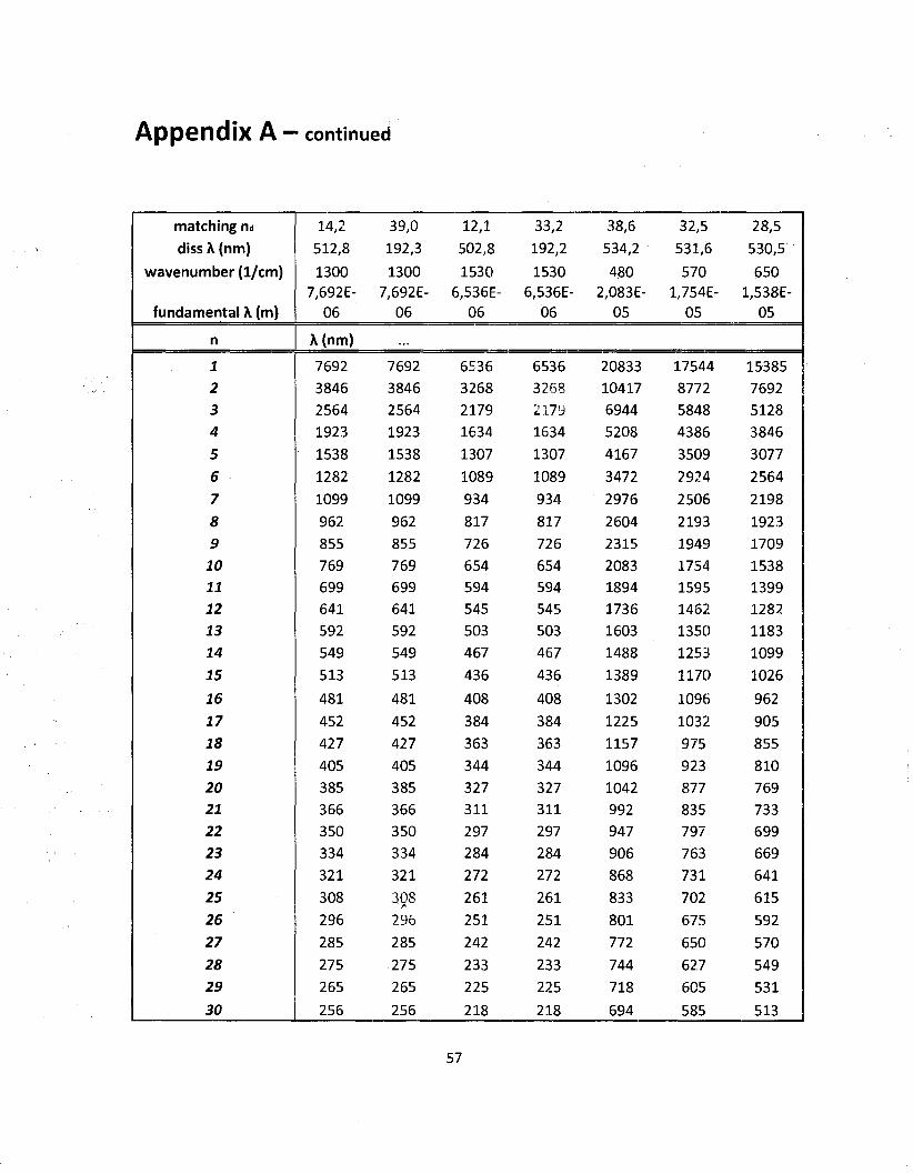
Append ix A - continued
matching rid
diss\(nm)
wavenumber (1/cm)
fundamental X (m)
n
1
2
3
4
5
6
7
8
9
10
11
12
13
14
IS
16
17
18
19
20
21
22
23
24
25
26
27
28
29
30
14,2
512,8
1300
7,692E-
06
39,0
192,3
1300
7,692E-
06
12,1
502,8
1530
6,536E-
06
33,2
192,2
1530
6,536E-
06
38,6
534,2
480 2,083E-
05
32,5
531,6
570 1,754E-
05
28,5
530,5
650 1,538E-
05
A(nm)
7692
3846
2564
1923
1538
1282
1099
962
855
769
699 641
592
549
513
481
452
427
405
385
366
350
334
321
308
296
285
275
265
256
7692
3846
2564
1923
1538
1282
1099
962
855
769 699
641
592
549
513
481
452
427
405
385
366
350
334
321
308
296
285
275
265
256
6536
3268
2179
1634
1307
1089
934
817
726
654
594
545
503
467
436
408
384
363
344
327
311
297
284
272
261
251
242
233
225
218
6536
3268
2179
1634
1307
1089
934
817
726
654
594
545
503
467
436
408
384
363
344
327
311
297
284
272
261
251
242
233
225
218
20833
10417
6944
5208
4167
3472
2976
2604
2315
2083
1894
1736
1603
1488
1389
1302
1225
1157
1096
1042
992
947
906
868
833
801
772
744
718
694
17544
8772
5848
4386
3509
2924
2506
2193
1949
1754
1595
1462
1350
1253
1170
1096
1032
975
923
877
835
797
763
731
702
675
650
627
605
585
15385
7692
5128
3846
3077
2564
2198
1923
1709
1538
1399
1282
1183
1099
1026
962
905
855
810
769
733
699
669
641
615
592
570
549
531
513
57
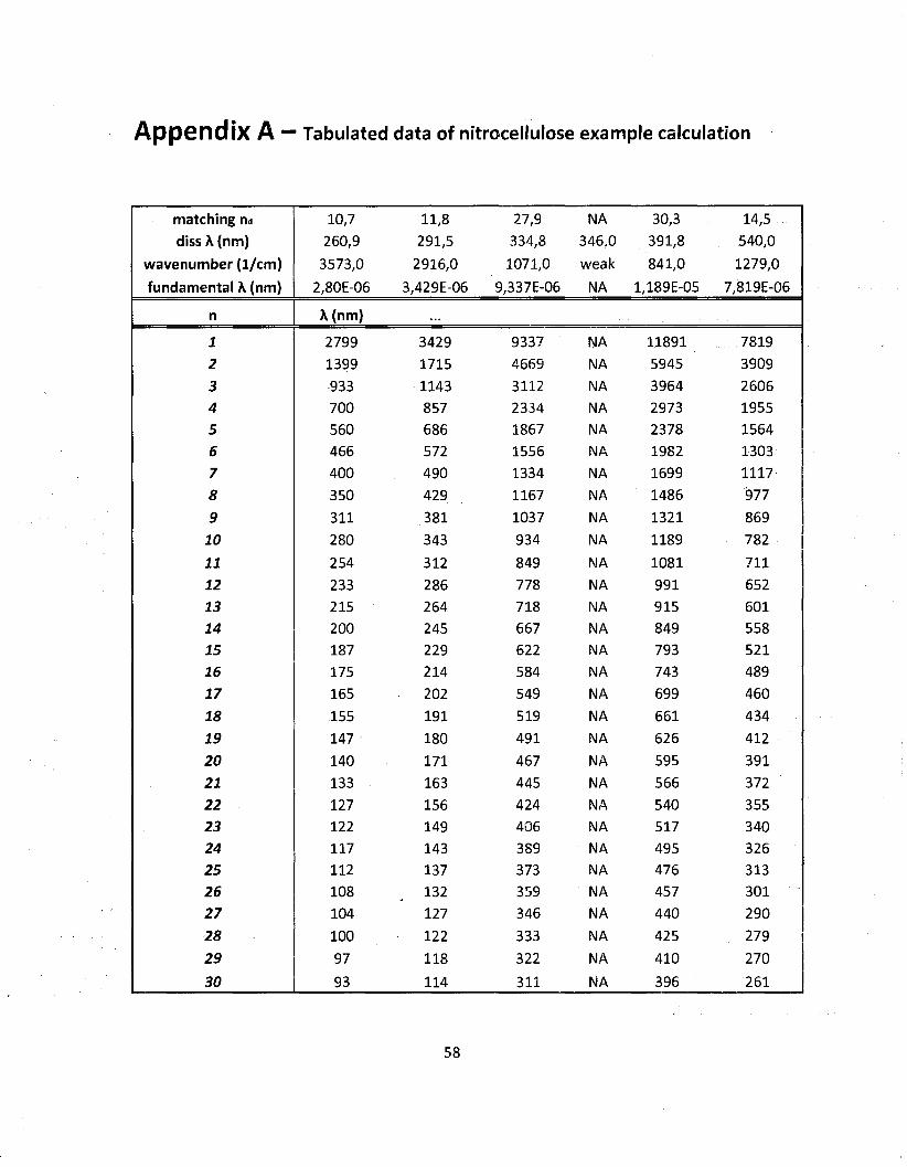
Ln
0
0
to
OJ
I-' !-»
J>
OJ
I-1 z > OJ
ID
en
NJ
CT
1
h-i
ID
•vl
l->
l-
>
oo
(JO
N
J N
J
Z > l-»
o
NJ
-vl
O
00
I-1 o
o
l-»
NJ
NJ
OJ
OJ
OJ
2 > J>
NJ
Ln
NJ
-vl
LO
l-»
O
-F»
l-»
NJ
•vl
Cn
z > O
NJ
ID
O
t-»
O
00
> i-»
OJ
M
U1
ID
Z > J>
171
•vl
OJ o
i-»
l-»
I-1
NJ
h->
O
J v
j
OJ
vj
OJ z > J>
•vl
cn
OJ
M
OJ
•IS.
(-»
H>
•vl
l-»
•P*
OJ
OJ
00
ID
z > •p*
ID
m
OJ
NJ en
l-»
NJ
NJ
l-»
J>
ID
O
CTi
z > i-»
vj
OJ
•p* o
M
l-»
NJ
•vl
l->
L
n
cn
J>
NJ
•pi
Z > Ln
-P
» o
OJ
Ln
L
n
h-»
O
J O
J
H-»
cn
OJ
tn
z > Ln
en
en
OJ
•vl
NJ
i-»
J> o
i-*
vj
l-»
-p*
en
•vl z > L
n
ID
Ln
OJ
ID
H>
to
l-i
-p»
vj
h-»
oo
o
ID
h-»
z > en
NJ en
J>
i-»
NJ
00
M
Ln
L
n
l-»
ID
l-»
Ln
ID
Z > cn
en
h-»
-P»
OJ
J>
NJ
H> en
un
NJ o
NJ
in
J>
ID
Z > cn
ID
ID
J> cn
O
Oi
i-»
vj
Ln
NJ
l-»
*>
00 *»
Z > •vl
J>
OJ
J> oo
ID
(J1
l-»
00
•vl
NJ
NJ
ID
cn
NJ
NJ z > -vl
ID
OJ
Ln
N
J I-
1
•Is,
NJ
O
O
NJ
J> Ln
en
cn
•vl z > oo
J>
ID
Ln
L
n
00
u>
NJ
h-»
L
n
NJ cn
•IS
.
vj
i-1
00 z > ID
Ln
cn
o
t-»
NJ
NJ
OJ
OJ
NJ
00 cn
•vl
•vl
oo
z > ID
ID
1-*
cn
on
NJ
i-t
NJ
Ln
J
>
OJ
H>
NJ
00
•P*
ID
z > 1081 vj
l->
l-
i
o
NJ
00 O
OJ
J>
OJ
ID
OJ
•P* z > 1189 vj oo
NJ
to
OJ
I-*
i-^
OJ oo
h->
1037 z > 1321 oo
cn
ID
00
OJ
Ln
O
J>
NJ
ID
1167 z > J> oo
cn
ID
vj
•vj
SI
4i
O o
•is
. ID
O
1334 z > 1699 1117
Cft
•F» cn
cn
on
•vl
NJ 1556 z > 1982 1303
Ul
on
cn
O
cn
oo
cn
1867 z > 2378 1564
•b
vj o
o
oo
m
-vl
2334 z > 2973 1955
U)
ID
OJ
OJ 1143 3112 z > 3964 2606
N) 1399 1715 cn
cn
ID
Z > 5945 3909
M 2799 3429 9337 z > 118 ID
7819
3 >»
"S" 3,
?
2 g"
mental >•
*••
»
3 3 "̂"̂
2,80E-06 _to
NJ
ID
E-0 cn
iP
OJ
OJ
•v! E-0 cn
Z > 189 E-0 en
Jv
l
oo
ID
E-0 cn
< 3 umber *M
o 3 *™^
OJ
vj
OJ O
NJ
ID
h-*
cn
O
107: o
0) 841 o
NJ
-vl
iP
o
Q.
3
atching n
issX(nm) **
NJ
M
g P
1o
^
NJ
M
ID
rr
{-* J
-1
"Ln °
°
g^
00
«
OJ cn
j,
o
oo
w
tn
_
o
^
o
w
> T5 fD
3 Q
_
> I H
0)
JT
C_
0) a.
Q.
0)
0)
o
o
O
VI m
fD
x 3 fD
r>
w_
o c_
0)
J* o'
3
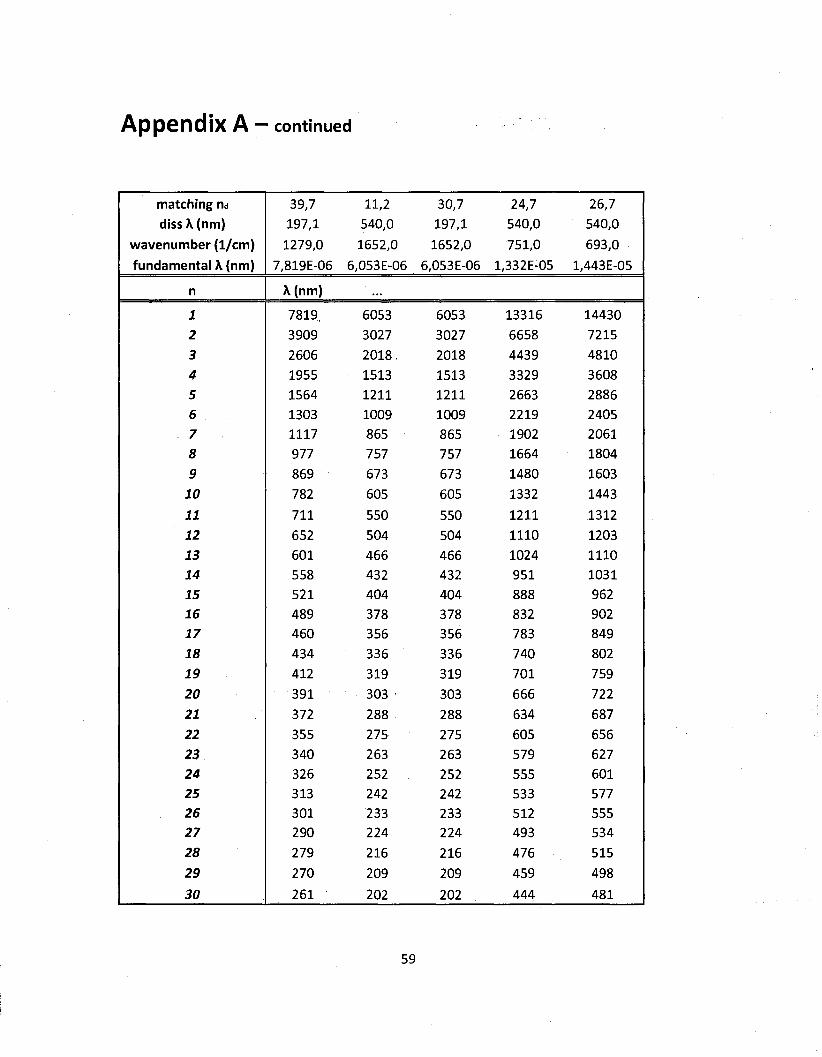
Appendix A — continued
matching rid
diss A (nm)
wavenumber (1/cm)
fundamental X (nm)
n
1
2
3
4
5
6
7
8
9
10
11
12
13
14
15
16
17
18
19
20
21
22
23 24
25
26
27
28
29
30
39,7
197,1
1279,0
7,819E-06
11,2
540,0
1652,0
6,053E-06
30,7
197,1
1652,0
6,053E-06
24,7
540,0
751,0
l,332E-05
26,7
540,0
693,0
l,443E-05
X(nm)
7819,
3909
2606
1955
1564
1303
1117
977
869
782
711
652
601
558
521
489
460
434
412
391
372
355
340
326
313 301
290
279
270
261
6053
3027
2018
1513
1211
1009
865
757
673
605
550
504
466
432
404
378
356
336
319
303 •
288
275
263
252
242
233 224
216
209
202
6053
3027
2018
1513
1211
1009
865
757
673
605
550
504
466
432
404
378
356
336
319
303
288
275
263
252
242
233
224
216
209
202
13316
6658
4439
3329
2663
2219
1902
1664
1480
1332
1211
1110
1024
951
888
832
783
740
701
666
634
605
579
555
533
512
493
476
459
444
14430
7215
4810
3608
2886
2405
2061
1804
1603
1443
1312
1203
1110
1031
962
902
849
802
759
722
687
656
627
601
577
555
534
515
498
481

A p p e n d i x B — FT-IR spectrum of nitrocellulose (Giasson, 2005)
Note: Spectra shown on the next page.

1)61
gft
Si
i)«
'&
NC
sec
Ber
gera
o
~~"-
~\ v.
V
y /
y^y
X
V
\ {
i.
I
ii
VI
**
•'
• '
I
H
1 /.
Kw
if
Tra
nsm
issi
on:/ -
Wav
enum
ber
(cn
vl)
File
# 7
= N
C S
EC
.TR
AN
SM
STT
AN
CE
Ber
gera
o
Pag
ed.
Y-Z
oom
CU
RS
OR
2006
-12-
21
10:3
2 R
es=4
;