1

A Simulation Game for Service-Oriented Supply Chain Management: Does Information Sharing Help Managers with Service Capacity Decisions?

To appear in the Spring 2000 (vol. 9, no. 1) issue of

The Journal of Production and Operations Management

Edward G. Anderson Management Department

CBA 4.202 The University of Texas at Austin

Austin, Texas 78712 Phone: (512) 471-6394 Fax: (512) 471-3937

Douglas J. Morrice MSIS Department

CBA 5.202 The University of Texas at Austin

Austin, Texas 78712-1175 Phone: (512) 471-7857 Fax: (512) 471-0587

Abstract

For decades, the Beer Game has taught complex principles of supply chain management in a

finished good inventory supply chain. However, services typically cannot hold inventory and can

only manage backlogs through capacity adjustments. We propose a simulation game designed to

teach service-oriented supply chain management principles and to test whether managers use

them effectively. For example, using a sample of typical student results, we determine that

student managers can effectively use end-user demand information to reduce backlog and

capacity adjustment costs. The game can also demonstrate the impact of demand variability and

reduced capacity adjustment time and lead times.

Keywords: Supply Chain Management, Teaching POM, System Dynamics, Business Games

2

1. Introduction

In response to growing demand from our corporate partners, the authors have recently

completed development of a Supply Chain Management course for our Executive Education

Program. In developing the course, the authors drew from many materials that have been

developed to support teaching this topic. For example, several new textbooks are either entirely

or partially devoted to this topic (Copacino 1997, Gattorna 1998, Handfield and Nichols 1998,

Ross 1998, Simchi-Levi, Kaminsky, and Simchi-Levi 1999). Additionally, in order to give the

clients a better “hands-on” feel for many supply chain management problems and how they

might be mitigated, the course includes a module featuring the famous Beer Distribution Game

developed at MIT almost thirty years ago (Sterman 1989b, Senge 1990). The Beer Game allows

teams of players to simulate the workings of a single product distribution supply chain in which

each player manages the inventory of either a retailer, wholesaler, distributor, or manufacturer.

In its original form, the game is set up as a physical simulation but it is also available as a

computer simulation (see, for example, Simchi-Levi, Kaminsky and Simchi-Levi 1999). Sterman

(1989b) extols the value of using simulated exercises to help the students gain first hand

knowledge of such things as the “bullwhip effect” (Forrester 1958, Lee, Padmanabhan, and

Whang 1997a, 1997b) and the benefits of lead-time reduction and information sharing.

However, many of our corporate partners operate inside of service supply chains, which behave

differently from finished goods inventory distribution chains. Although these clients might find

the Beer Game interesting and we might be able to extrapolate some principles to fit their

business environment, the game is not ideal. In particular, service supply chains typically do not

have inventory stocks that are replenished directly through order placements, but rather only

3

backlogs that are managed indirectly through service capacity adjustments. The Beer Game

models the former sort of supply chain quite well, but is not as representative of the latter. For

example, the Beer Game assumes for reasons of pedagogical simplicity an infinite manufacturing

capacity. While this assumption is reasonable when simulating a distribution supply chain, it is

problematic in a service supply chain. Consequently, the authors have developed a game that

more closely resembles service supply chains and the types of decisions made within these

contexts.

In this paper, we develop a supply chain game with three main features:

i) The supply chain has multiple, potentially autonomous, players performing a sequence of

operations.

ii) Finished goods inventory is not an option because the product or service is essentially

make-to-order.

iii) Each player manages order backlog by adjusting capacity.

The game we develop is called the Mortgage Service Game. Like the Beer Game, we chose

to model a specific application as opposed to using a generic model. A specific application has

much greater pedagogical value because participants are more likely to assume the roles within

the game and make the simulation more closely mimic reality. Additionally, the mortgage

service supply chain provides a realistic application that encompasses all the features listed

above. The principles learned from this game can be easily generalized to other industries that

have supply chains with similar features (see, for example, Wheelwright 1992).

Aside from being an integral part of a service supply chain course, a second major use of the

game is for research and assessment purposes. In particular, how well do the students apply the

supply chain principles that they are taught in class? For instance, can the students effectively

4

use end-user demand information to improve their performance? And if they can, how much

will they benefit? The Mortgage Service Game can help researchers answer these sorts of

research questions. To demonstrate this use, we present in this paper a sample of typical student

results from classroom experience in playing the Mortage Service Game. We analyze the results

to determine how effectively student managers can use end-user demand information to reduce

backlog and capacity adjustment costs; thus ameliorating the “bullwhip effect.” From the

analysis, we determine that indeed students do improve their performance significantly by using

end-user demand information, both in a statistical sense and relative to an “optimal” benchmark.

This is an encouraging result given the demonstrated difficulty with which managers cope with

dynamically complex environments (Sterman 1989b).

The remainder of the paper is organized in the following manner. Section 2 contains a

description of the Mortgage Service Game simulation model. Section 3 briefly describes the

behavior of the Mortgage Service supply chain. Section 4 outlines various teaching strategies

that can be used to describe principles in capacity management with and without end-user

demand information. Additionally, this section also presents the results from classroom use of

the simulation game. Section 5 discusses extensions to the service game and contains other

concluding remarks.

2. The Mortgage Service Game

To make the service supply chain game concrete, we will use it to represent a simplified

mortgage approval process from application submission through approval. The model’s purpose

is to capture the essential elements of reality common to most service supply chains rather than

perfectly simulate the mortgage industry. As such, some supply-chain complexities idiosyncratic

to the mortgage industry are not modeled in the interest of pedagogical simplicity. The model is

5

currently implemented in the Vensim© Simulation Package (Ventana Systems Inc., 1998) and

Ithink Simulation Package (Richmond and Peterson, 1996). Figure 1a depicts the basic logic of

the model in the form of a Vensim block diagram. An equivalent Ithink model is used to conduct

the game in a classroom setting (see Section 3.1 for more details).The graphical user interface of

an Ithink model is given in Figure 1b.

(insert Figure 1a here)

Figure 1a: Block Diagram of The Mortgage Service Game

(insert Figure 1b here)

Figure 1b: Graphical User Interface of The Mortgage Service Game

Each mortgage application passes through four stages: initial processing (that is filling out

the application with a loan officer), credit checking (confirmation of employment and review of

credit history), surveying (a survey of the proposed property to check for its value, as well as any

infringements upon zoning laws or neighboring properties), and title checking (ensuring that the

title to the property is uncontested and without liens). Mechanically, all the stages operate in an

identical manner, so we will describe here only the survey section of the model as an example of

each stage’s processing. As each application is checked for the credit worthiness of its applicant

(credit checking in the diagram), the application flows from the backlog of credit checks (Credit

Check Backlog) to join the backlog of surveys (Survey Backlog). Each week, based on the

backlog of surveys—which is the only information available to the player controlling the survey

stage of the system when using a decentralized strategy—the player sets the target capacity of

the system by deciding to hire or fire employees: in this case, surveyors. However, it takes time

to actually find, interview, and hire or, conversely, to give notice and fire employees; so the

actual Survey Capacity will lag the Target Survey Capacity by an average of one month. Those

6

surveyors currently in the employ of the survey company will then carry out as many surveys as

they can over the next week. Finally, as each application’s survey is completed (surveying), the

application will then leave the Survey Backlog to join the next backlog downstream—in this

case, the Title Check Backlog. Each of the other four stages functions analogously.

In real life, of course, the purpose of each of these checks is to eliminate those applications

that are too risky. However, again for reasons of pedagogical simplicity, we will assume that

each application is ultimately approved. This is reasonable because, despite the fact that a

random survival rate for each stage does indeed complicate real-life management of the chain,

the primary dynamic control problems derive from other sources. In particular, the largest

problem results from each stage of the process generally being managed by a separate company.

Each of these companies controls its own individual capacity; however, it typically only sees its

own backlog when making the decision, not the global new application rate or other stages’

backlogs. This creates something akin to the bullwhip effect (Lee et al. 1997b) seen in the Beer

Game (Sterman 1989b), albeit here the inventories controlled are strictly backlogs. Also, as in

many real life services, there is no way for a player to stockpile finished goods inventory in

advance as a buffer against fluctuating demand. Rather, each stage must manage its backlog

strictly by managing its capacity size, that is the number of workers it employs.

Mathematically, the structure for each stage of the process is as follows (Let stages 1, 2, 3,

and 4 refer respectively to the application processing, credit checking, surveying, and title

checking stages):

titititi rrBB ,,1,1, −+= −+ (1)

) ,min( ,1,,, titititi rBCr −+= (2)

7

where B(i,t), C(i,t), and r(i,t) refer respectively to the backlog, the capacity, and the completion

rate at stage i on day t. Note that r(0, t) represents the new application start rate, which is

determined exogenously (for example, by the instructor). In the game, this variable remains at a

constant level over an initial period of time. At a certain point in time r(0,t) steps up to a higher

level where it remains constant for the remainder of the game. For simplicity, we will assume

that each employee has a productivity of one application per day. Because of this simplifying

assumption, the completion rate of applications at any stage is constrained to the minimum of the

backlog plus any inflow from the previous stage (if material is constraining processing) or the

capacity (the more typical case). Each stage’s backlog is initialized at the beginning of the game

to λ[r(i,0)] where λ is a constant representing the average nominal delay required to complete a

backlogged application. Each stage’s capacity is initialized at r(i,0) so that the backlogging and

completion rates at each stage are in balance (see Equations 3 and 4 below). Hence, if there were

no change in the application start rate, there would never be a change in any backlog, capacities,

or completion rates throughout the service chain.

At the beginning of each week (i.e. every 5 business days), each company can change its

target capacity by deciding to hire or lay off employees. However, it takes time to advertise,

interview, and hire employees; so the rate of capacity change is given in Equation 3.

)CC(CC t,i*

t,it,it,i −+=+ τ1

1 . (3)

The target capacity C*(i, t) set by the player is restricted to be nonnegative. For purposes of this

game, τ, the capacity adjustment time, is set to one month, that is 20 business days (which is, in

reality, a bit optimistic if large hiring rates are required). In essence, each stage’s capacity will

move one twentieth of the gap from its current value toward its target each day. Thus, the

capacity adjustment occurs not in a lump on any particular day but rather stretches out over many

8

days. For example, if the target capacity suddenly increases by a one-time fixed amount, 5% of

the increase will arrive the next day; 5% of the remaining 95% gap will arrive on the second day,

and so on in an exponentially decreasing manner. This translates into an average lag for hiring

(or firing employees) of 20 business days. If for some reason, however, the player makes

another capacity change before the original adjustment is complete, the old target will be thrown

out, and the next day capacity will begin to adjust from its current value toward the new target.

If for some reason a player cannot be found for each stage, the target capacity decision will

be made as follows:

λ

t,i*t,i

BC = if (t modulo 5) = 0 (4)

*t,i

*t,i CC 1−= otherwise.

Thus, each week the target capacity for each stage will be set directly proportional to the stage’s

current backlog B(i,t) and inversely proportional to the nominal service delay time λ. This is not

meant to be an optimal policy in any sense; however, it seems to reflect reasonably well how real

players make decisions in capacity management games (Sterman 1989a). Thus, if the

application start rate is unvarying, the long-run average application will take λ weeks to

complete per stage. One can of course vary λ either by stage or over time to make the game

more complex.

The goal of each team of four players (or each individual depending on the scenario) is to

minimize the total cost for the entire supply chain resulting from employee salaries and service

delays. Each employee will cost $2000 to hire or lay off and $1000 per week to employ (or $200

per application when fully utilized). Each backlogged application costs $200 per week in

potential customer alienation.

9

Although the management of capacity at each stage in the mortgage service supply chain

may be well understood (e.g., Equations 3 and 4), backlog (and other performance measures)

may exhibit very complex behavior since the stages do not function independently but are linked

in a supply chain. Therefore, we devote the next section to describing the system behavior and

the output generated by the simulation model in Figure 1.

3. System Behavior

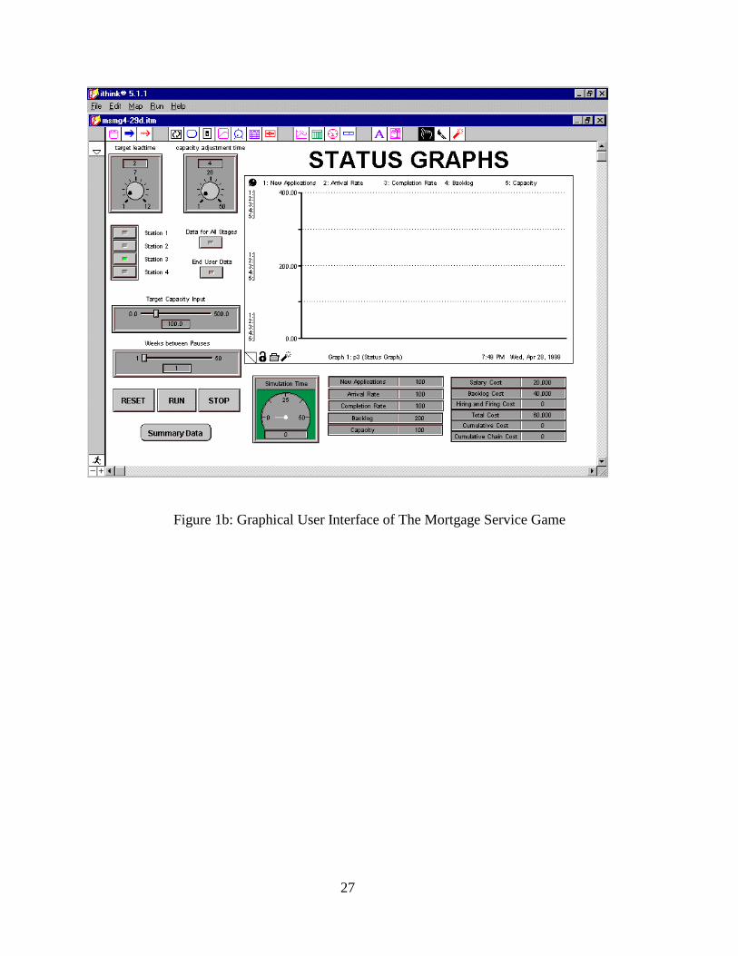
To illustrate system behavior, let us examine the response of the initial applications

processing rate to a step increase of 35% in application starts (Figure 2). More specifically,

r(0,t) remains at 20 starts per day until after 8 weeks, when it jumps to 27 starts per day. The

number of starts per day then remains constant at 27 until the end of the game in week 100. Note

that in this section, the capacity adjustment time τ is set to 4 weeks and the target backlog delay

λ is set to 2 weeks. Also, note that we are employing here the non-optimal—but often realistic—

capacity adjustment heuristic described in Equation 4. We chose this scenario because it provides

a good illustration of the complexities that arise even in this relatively simple supply chain.

(Insert Figure 2 about here)

Figure 2: Applications Processing for All Stages Over Time (i.e., t,ir )

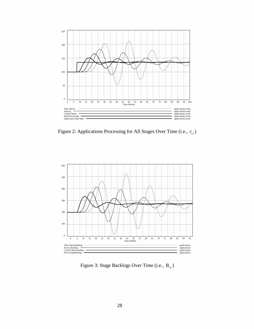
(Insert Figure 3 about here)

Figure 3: Stage Backlogs Over Time (i.e., t,iB )

Immediately after the increase in starts after 8 weeks, the processing backlog increases

because processing capacity lags behind the increase in application starts (Figure 3). After a

10

week’s delay, the processing capacity will begin to adjust to the increase in the backlog.

However, the backlog will still increase until week 13.

(Insert Figure 4 about here)

Figure 4: Stage Capacities Over Time (i.e., t,iC )

In week 13, the processing capacity, and hence the application processing rate, catches up

with the application starts. But the capacity must actually overshoot its final settling point at 135

applications per week (Figures 2 and 4) because, during the time that processing capacity lagged

application starts, the backlog has increased by more than 65% (Figure 3). Thus, the capacity

overshoot is necessary in order to reduce the backlog back to its new equilibrium value. In fact,

the capacity will continue to increase as long as the backlog exceeds the target delay of two

week’s processing, which will continue until week 17. From this point on, the capacity begins to

reduce, but it still exceeds the new start rate; hence, the backlog will itself drop below its final

equilibrium and keep dropping until week 23. At this time, the amount of capacity required to

process the backlog in two weeks is less than the application start rate. Thus, despite the fact that

the backlog is growing, the capacity will continue to drop until week 27 when the backlog once

again exceeds its final equilibrium value. From this point, the application capacity and

processing will increase to begin another, albeit less pronounced, cycle.

Because the credit check stage in this scenario has no access to end-user information, it only

sees the output from the initial processing stage. As described, there is a lag between when end-

user information increases and capacity arrives at the initial processing stage. Thus, the peak in

backlogged applications from initial processing will arrive at credit check delayed even beyond

the target backlog delay of 10 business days. This delay prevents timely reaction from the credit

11

check player. Because of the bullwhip effect in initial applications processing, the applications

will also arrive at credit checking with a peak quantity greater than that which arrived at initial

processing (see the initial applications processing output week 17 in Figure 2). Thus, the

bullwhip process described in the initial application stage will repeat itself with greater force at

the credit check stage. Further, when the downturn in initial processing arrives in weeks 23

through 31, the credit check stage does not know that this is result of the first stage’s over-

capacitization. Hence, credit checking will mistakenly believe that end-user demand has dropped

and adjust its capacity downward more vigorously than it might otherwise. Credit checking

capacity reductions will continue even after the backlog begins to rebuild at initial processing

beyond its new equilibrium (week 27). Since the output from initial processing has a greater

maximum amplitude than the application start rate followed by a series of ever-dampening

cycles, credit checking’s behavior will continue to repeat, albeit with ever-lessening force.

The same basic repeating cycles of backlog, capacity, and processing will occur for the same

reasons at the survey and title check stages, though the cycles are increasingly more lagged and

forceful at each stage.

4. Teaching Strategies

The Mortgage Service Game is played under two main strategies: decentralized and new

application starts information strategy. Sections 2 and 3 describe the game in terms of the

decentralized strategy. Each stage operates autonomously and makes its capacity decisions based

on its own backlog. In the new application starts information strategy, each stage makes capacity

decisions based on its own backlog and the new applications rate. In other words, each stage

gains more visibility by being able to observe end user demand in each time period. For those

stages at which the computer makes the target capacity decision, Equation 4 changes to:

12

λ

αα t,it,0

*t,i

B)1(rC −+= , if (t modulo 5) = 0 (5)

*t,i

*t,i CC 1−= , otherwise

where 10 << α . The degree to which each stage in the chain bases its target capacity on the new

application rate is determined by the magnitude of α . In this case, the same value for α is used

for all stages that set target capacity using Equation 5. A more complicated version of the game

could be designed to permit a different α for each stage.

4.1 Classroom Use

We conducted mortgage service simulation exercises in two courses. One course contained

seventeen masters’-level students (MBA and Master of Science in Engineering) studying

operations simulation modeling. These students were technically oriented and the Mortgage

Service Game exercise was used to teach concepts in supply chain management and operations

modeling in the service sector. The other course had 23 students, mostly MBAs, studying supply

chain management. Although these students were less technically oriented, they were familiar

with several supply chain concepts including the beer game (both physical and computerized)

and the bullwhip effect in the management of supply chain inventories.

4.1.1 Set-up

Both classes played a stand-alone PC version of the Mortgage Service Game. In this version

of the game, each team of students managed only the survey stage in the chain, leaving the

computer to manage the remaining stages. Teams were assigned to an intermediate stage in the

supply chain in order to illustrate the dynamics resulting from information and capacity

adjustment lags. In order to mitigate the perception of the computer performing “black box”

functions, we provided students with complete details about the operations of the game at all

13

stages (i.e., Equations (1) through (5)). In fact, the only information the students were not given

was how and when the demand stream changed. For all of the exercises described below, we

used the following demand stream: r(0,t) remains at 20 starts per day until after 8 weeks, when it

jumps to 27 starts per day. The number of starts per day then remains constant at 27 until the end

of the game in week 50. Most teams consisted of two students. However, a few teams had three

members, and in one case, we had a single-student team.

We used the Mortgage Service Game to demonstrate two main points. The first point was to

illustrate the supply chain dynamics resulting from information and capacity adjustment lags.

The second point was to illustrate the impact of end user demand information. Therefore, during

the class each team performed two exercises with the Game: one was to manage capacity and

backlogs at the survey stage without new applications information and the other was to manage

the stage with that information. The following instructions were given at the beginning of class:

“We will play the game twice: once with no new applications information provided to the

property survey stage and once with new applications information provided to the property

survey stage. Some of the groups will start with new applications information in the first round.

The remaining groups will start with no new applications information. New applications

information availability is reversed in the second round. The target lead-time equals two weeks

(or ten days) and capacity adjustment time equals four weeks (or 20 days). For the computer-

controlled stages, the weight (i.e., the α value) on the new application rate will be set equal to

zero when no new applications information is provided and 0.5 when new applications

information is provided. New applications will begin at 20 per day (or 100 per week) but then

will change by an unspecified amount at an unspecified point in time. Hence, there is no use

trying to anticipate the change and the timing of the change from the previous run. Each stage

14

(including the survey of property stage) will begin with a backlog of 200, capacity of 20 per day

(or 100 per week), and target capacity of 20 applications per day (or 100 per week), i.e., each

stage (and hence the entire supply chain) will begin in equilibrium. Each game will be conducted

for 50 rounds where each round corresponds to one week.” Hence the students were given

complete information on what they were to do and what the computer would be doing with

respect to each exercise. We chose these parameters for the classroom exercises based on

simulation results similar to those found in Anderson and Morrice (1999). These results show

that with the parameters used, rational decision making behavior will lead to improved

performance with new applications information. Additionally, since we conducted both exercises

in one 75-minute period, each exercise was limited to 50 weeks.

Prior to conducting the exercises, we gave a complete description of all information

displayed on the graphical user interface of the iThink model in Figure 1b. “Target Leadtime”

and “Capacity Adjustment Time” are displayed in the top left-hand corner of the screen. The

players cannot change these parameters. Just below these parameters, one can select the station

managed by the student team. This was set to “Station 3” for both exercises. “The Data for All

Stages” allows the administrator of the game to change the demand stream. The players cannot

change this setting after the game starts. If the “End User” data button is selected, then new

applications rate data is displayed during the game. Again, the players cannot change this setting

after the first round of the game is played. The “Target Capacity Input” lever allows the players

to control the target capacity. “Weeks between Pauses” determines the duration of each round of

the game. We set this to one, and it cannot be changed by the players. The “Reset” button resets

the game, the “Run” button advances each round, and the “Stop” button stops the game. The

“Summary Data” button opens a window that provides summary data at the end of each game.

15

The “Simulation Time” dial displays the current time of the simulation. The graph and a table

directly below the graph display the New Applications rate (in the exercise in which new

applications information is provided). Additionally, they provide Arrival Rate, Completion Rate,

Capacity, and Backlog for the current stage being managed by the players (in both our exercises,

the survey stage). The final table contains the costs results based on the cost structure described

in Section 2.

4.1.2 Analysis

We collected data from seven teams in the operations simulation class and ten teams in the

supply chain management class. Since each team played the game twice, a total of 34 data

records were generated. Each record contains data on the mean backlog, standard deviation of

the backlog, and cumulative cost at each stage. The standard deviation of the backlog can be

used to illustrate supply chain dynamics and a bullwhip effect. The cumulative costs can be used

to demonstrate the impact of new applications information. The players recorded these data after

each game from the “Summary Data” window. Therefore, they received direct feedback on

supply chain dynamics and the impact of new applications information.

In what follows, we performed several statistical tests that rely on the data being normally

distributed. In all cases, the hypothesis of normality was not rejected based on the Chi-square,

Kolmogorov-Smirnov, and Anderson-Darling in BestFit software (Palisade, 1996). We must

point out that since these data sets are quite small, the power of the test for rejecting the null

hypothesis of normality is small.

Since the exercises in both classes were run under the same experimental conditions (i.e.,

using the same lab and the same instructions), we decided to pool the results. Further support for

pooling the data resulted from statistical tests on the difference between cumulative costs for the

16

last two stages with and without new applications information (from now on these data will be

referred to as the cumulative cost differences). We consider these data the best indicators of

performance because the teams managed the survey stage and therefore only impacted the

performance of the last two stages in the supply chain. Neither an F-test on the equality of

variances, nor a two-sample t-test on the equality of means on these data detected significant

differences at the five-percent level.

On the pooled data we conducted a paired t-test on these data to determine whether or not the

players’ performances were significantly better when new applications information was

available. Table 1 contains highly significant results: the paired t-test shows that, on average,

players had a significantly lower mean cumulative cost when new applications information was

available.

Another way to assess the players’ performance with and without information is to compare

the difference between the mean cumulative costs in Table 1 with the difference between

cumulative costs that could be obtained using an optimal strategy. The optimal strategy uses

Equation (5) with an optimally selected value for α to manage survey stage target capacity (and

α equal 0.5 for all other stages) when new information is available and Equation (4) to manage

target capacity at all stages without information. It is important to note that this comparison is

not perfect since the players were not limited to selecting α but could set the actual target

capacity. However, many players indicated that they were following a policy closely related to

Equations (5) and (4) with and without information, respectively (please see the discussion of

player strategies below). To select α optimally for the survey stage, we constructed a non-linear

program to minimize total cumulative cost over all stages. A grid search and the GRG2 solver in

Microsoft Excel was used to select the α optimally for the survey stage. The cumulative cost

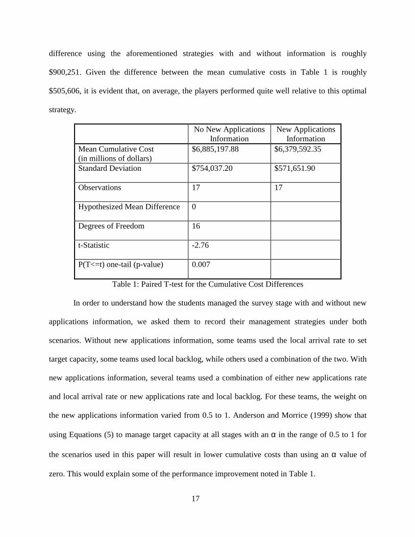
17

difference using the aforementioned strategies with and without information is roughly

$900,251. Given the difference between the mean cumulative costs in Table 1 is roughly

$505,606, it is evident that, on average, the players performed quite well relative to this optimal

strategy.

No New Applications Information

New Applications Information

Mean Cumulative Cost (in millions of dollars)

$6,885,197.88 $6,379,592.35

Standard Deviation $754,037.20 $571,651.90

Observations 17 17

Hypothesized Mean Difference 0

Degrees of Freedom 16

t-Statistic -2.76

P(T<=t) one-tail (p-value) 0.007

Table 1: Paired T-test for the Cumulative Cost Differences

In order to understand how the students managed the survey stage with and without new

applications information, we asked them to record their management strategies under both

scenarios. Without new applications information, some teams used the local arrival rate to set

target capacity, some teams used local backlog, while others used a combination of the two. With

new applications information, several teams used a combination of either new applications rate

and local arrival rate or new applications rate and local backlog. For these teams, the weight on

the new applications information varied from 0.5 to 1. Anderson and Morrice (1999) show that

using Equations (5) to manage target capacity at all stages with an α in the range of 0.5 to 1 for

the scenarios used in this paper will result in lower cumulative costs than using an α value of

zero. This would explain some of the performance improvement noted in Table 1.

18

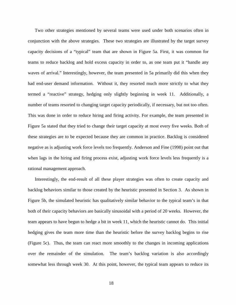
Two other strategies mentioned by several teams were used under both scenarios often in

conjunction with the above strategies. These two strategies are illustrated by the target survey

capacity decisions of a “typical” team that are shown in Figure 5a. First, it was common for

teams to reduce backlog and hold excess capacity in order to, as one team put it “handle any

waves of arrival.” Interestingly, however, the team presented in 5a primarily did this when they

had end-user demand information. Without it, they resorted much more strictly to what they

termed a “reactive” strategy, hedging only slightly beginning in week 11. Additionally, a

number of teams resorted to changing target capacity periodically, if necessary, but not too often.

This was done in order to reduce hiring and firing activity. For example, the team presented in

Figure 5a stated that they tried to change their target capacity at most every five weeks. Both of

these strategies are to be expected because they are common in practice. Backlog is considered

negative as is adjusting work force levels too frequently. Anderson and Fine (1998) point out that

when lags in the hiring and firing process exist, adjusting work force levels less frequently is a

rational management approach.

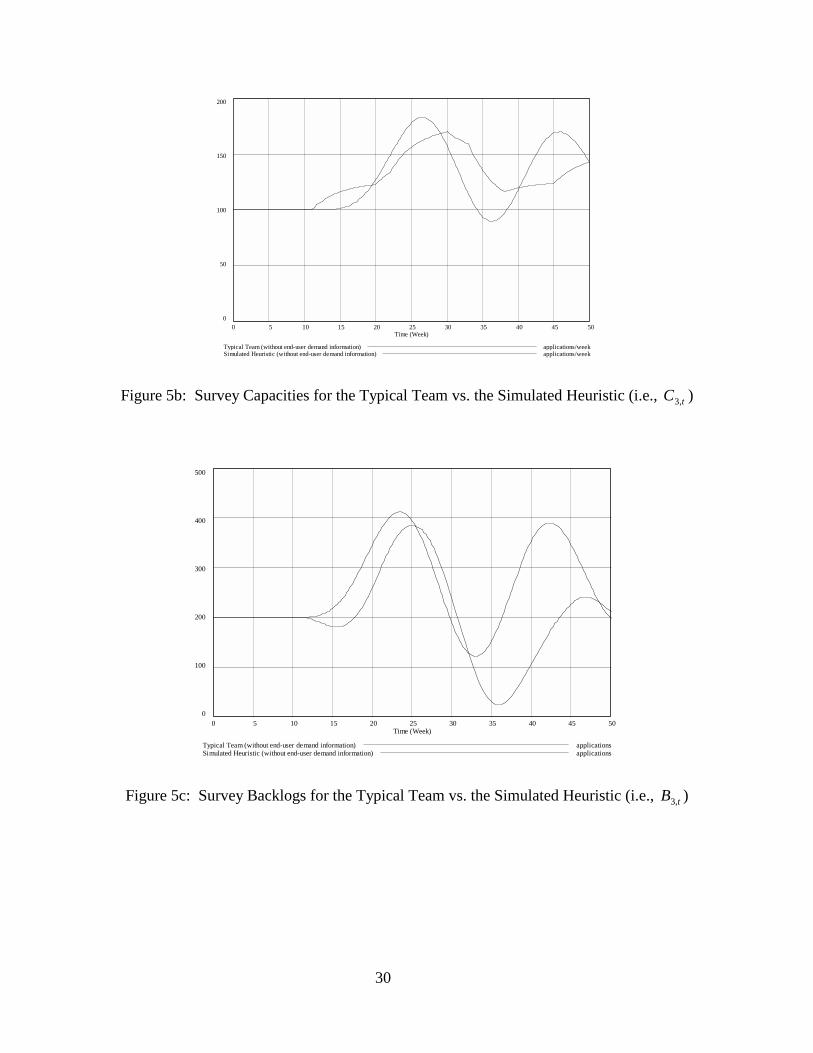
Interestingly, the end-result of all these player strategies was often to create capacity and

backlog behaviors similar to those created by the heuristic presented in Section 3. As shown in

Figure 5b, the simulated heuristic has qualitatively similar behavior to the typical team’s in that

both of their capacity behaviors are basically sinusoidal with a period of 20 weeks. However, the

team appears to have begun to hedge a bit in week 11, which the heuristic cannot do. This initial

hedging gives the team more time than the heuristic before the survey backlog begins to rise

(Figure 5c). Thus, the team can react more smoothly to the changes in incoming applications

over the remainder of the simulation. The team’s backlog variation is also accordingly

somewhat less through week 30. At this point, however, the typical team appears to reduce its

19

target backlog goal from its initial position at 200 applications, thus making comparison with the

heuristic problematic. In summary, the heuristic does seem to capture much, though not all, of

the typical team’s behavior, at least for the case without end-user information.

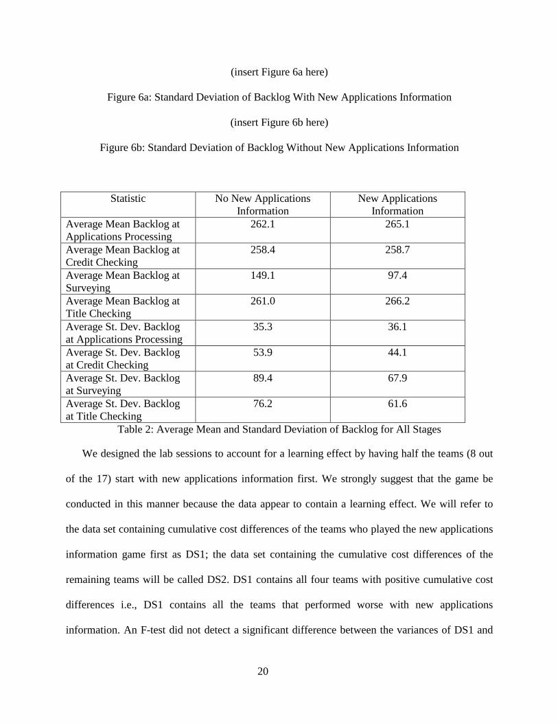
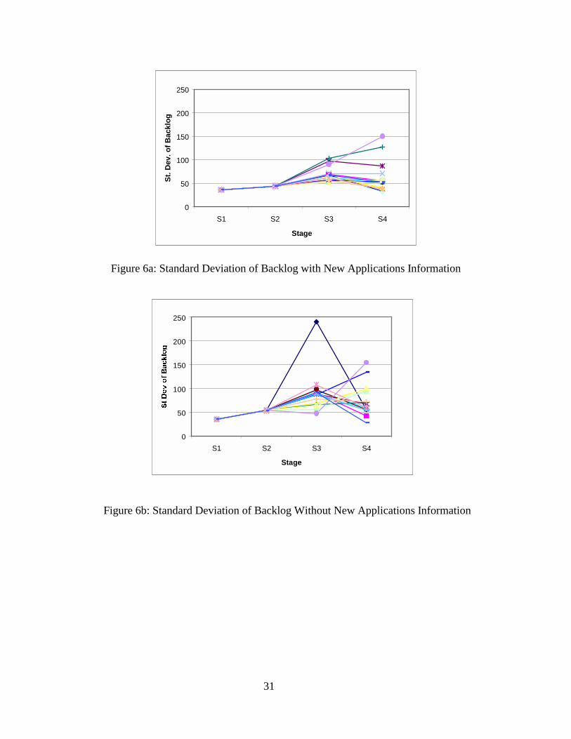
At a more macro level of analysis, Figures 6a and 6b contain plots of standard deviation of

backlog at all stages for the 17 teams with and without new applications information,

respectively. The x-axis for each plot lists the four stages in the supply chain denoted by S1

(initial processing) through S4 (title checking). Each plot contains a line graph for each team that

shows their standard deviation of backlog across all stages. Table 2 contains the average (over

the 17 teams) mean and standard deviation of the backlog for the survey and title checking stages

with and without new applications information.

A couple of observations can be made from these data. First, the bullwhip effect is evident

from the increasing average standard deviation of the backlog as one moves down the supply

chain under both scenarios. Note that the average standard deviation of the backlog drops at the

title stage because, in general, players manage the survey stage with excess capacity or with

lower than average backlog (compare average mean backlog at the surveying stage with this

statistic at other stages in Table 2). This result is consistent with the strategy that several teams

stated they were using. Second, we observe that the bullwhip effect is somewhat mitigated by

having new applications information (compare the average standard deviation of the backlogs for

both scenarios in Table 2). Note that due to the size of the data set, we were not able to establish

statistical significance on our observations about the data in Table 2 and Figures 6a and 6b. Our

comments are based on trends observed in these data.

20

(insert Figure 6a here)

Figure 6a: Standard Deviation of Backlog With New Applications Information

(insert Figure 6b here)

Figure 6b: Standard Deviation of Backlog Without New Applications Information

Statistic No New Applications Information

New Applications Information

Average Mean Backlog at Applications Processing

262.1 265.1

Average Mean Backlog at Credit Checking

258.4 258.7

Average Mean Backlog at Surveying

149.1 97.4

Average Mean Backlog at Title Checking

261.0 266.2

Average St. Dev. Backlog at Applications Processing

35.3 36.1

Average St. Dev. Backlog at Credit Checking

53.9 44.1

Average St. Dev. Backlog at Surveying

89.4 67.9

Average St. Dev. Backlog at Title Checking

76.2 61.6

Table 2: Average Mean and Standard Deviation of Backlog for All Stages

We designed the lab sessions to account for a learning effect by having half the teams (8 out

of the 17) start with new applications information first. We strongly suggest that the game be

conducted in this manner because the data appear to contain a learning effect. We will refer to

the data set containing cumulative cost differences of the teams who played the new applications

information game first as DS1; the data set containing the cumulative cost differences of the

remaining teams will be called DS2. DS1 contains all four teams with positive cumulative cost

differences i.e., DS1 contains all the teams that performed worse with new applications

information. An F-test did not detect a significant difference between the variances of DS1 and

21

DS2. However, a two-sample t-test did detect a significant difference between the means of these

two data sets at the five percent level (the p-value was 0.011).

It is possible that the above learning effect is due, at least in part, to an anticipation effect. In

both games, the players faced the same demand. Hence, after the first game, the players could

just anticipate the same demand pattern for the second game. We argue that this did not happen

in our game for two reasons. First, we explicitly told the students not to anticipate the demand

change and its timing from the previous run since these amounts were randomly selected on each

run (see Section 4.1.1). Second, an anticipation effect was not apparent in the data. To test this,

we compared the results for the without information games played first with results from the

without information games played second and found no significant difference. If an anticipation

effect were present one would expect to observe better second round results since players have

already seen the demand stream from the first round in the game with information.

Incidentally, the learning effect mentioned above was completely due to the difference in the

results for the games with information (i.e., results for the games with information played in the

second round were significantly better than results for the games with information played in the

first round). These results are less likely due the anticipation effect since a second round game

with information is proceeded by a first round game without information that does not explicitly

provide the new applications information. We argue that the results are more likely to be due to a

learning effect because managing with more information choices requires experience.

Further analysis and control of both learning and anticipation effects can be performed using

more comprehensive experimental designs (generally requiring larger data sets) than we have

considered in this analysis. This will be part of our future research.

22

4.1.3 Feedback

We suggest that a feedback session be conducted after the Mortgage Service Game exercises.

We found that providing results similar to those given in Section 4.1.2 is of great pedagogical

value. Game participants learn from their own results as well of the results of others.

Additionally, they get the opportunity to observe trends in the data, which is especially important

for those who had worse performance with new applications information.

4.1.4 Other Exercises

If time permits (or there are a large number of participants who can be subdivided into

smaller groups), other exercises can be conducted with the current version of the Mortgage

Service Game. In particular, one can look at different capacity adjustment times (i.e., different

values for τ) and different values for average nominal delay (i.e., different values for λ).

5. Discussion and Conclusions

In this paper, we have introduced a simulation game to teach service-oriented supply chain

management principles. The Mortgage Service Game provides a realistic application with results

that can be generalized. We envision using this game instead of the Beer Game with participants

who have supply chains without finished goods inventory. However, it could be used to

complement the Beer Game in a supply chain management course that covers both finished

goods inventory management and service management. Furthermore, the Mortgage Service

Game can be used to illustrate supply chain management principles in a make-to-order

environment.

As future research and development, we plan to embellish this game in a number of ways.

First, we plan to develop a web-based version of the game. As we have demonstrated, the PC

23

version of the game can be an effective tool for teaching management strategies in a service

supply chain. However, the PC version limits the game to one team playing with the computer.

An initial web version of the game would be the same as the PC version except that the former

would permit up to four teams to play with each other in the same game. The computer using

Equation 4 (or Equation 5) to set target capacity would only play stages not covered by a team.

Subsequent versions of the PC and web-based games will be extended to include a global

information strategy in which all backlog and capacity information is shared across all stages, a

collaborative strategy in which global information is available and capacity can be shared across

all stages, and a centralized management strategy in which global information is available and a

single team manages capacity for all stages. Ultimately, the web-based version will permit us to

develop a virtual environment for constructing supply chain exercises that will closely mimic

reality.

We also plan to embellish the demand stream (i.e., the new application starts) so that it can

be both non-stationary and random. Adding randomness would enhance playing multiple rounds

since the demand stream would not be exactly the same each time the game is restarted.

However, we must point out that randomness in demand can and should be carefully controlled

in such games since noisy demand could mask variance propagation by the system. One major

advantage of a simulation environment is the ability to select common random number streams

for the demand so that all participants would face exactly the same noisy demand conditions.

Finally, this paper provides an introduction to players’ behavior during the Mortgage Service

Game. We plan to conduct further experiments and a statistical analysis similar to Sterman

(1989a, 1989b). These efforts should provide significant pedagogical insights beyond those

reported in this paper.

24

Acknowledgements

Professor Vishwanathan Krishnan of the Management Department at the University of Texas at

Austin also contributed to the development of the Supply Chain Management course for the

Executive Education Program. We would also like to acknowledge the contributions of Dr.

David Pyke and of two anonymous referees, whose suggestions improved this paper

immeasurably.

References

ANDERSON, E.G. AND C.H. FINE (1998), "Business Cycles and Productivity in Capital

Equipment Supply Chains" in Quantitative Models for Supply Chain Management, S. Tayur,

M. Magazine, and R. Ganeshan (eds.), Kluwer Press, Boston, 381-415.

ANDERSON, E. G. AND D. J. MORRICE (1999), “A Simulation Model to Study the Dynamics

in a Service-Oriented Supply Chain,” to appear in Proceedings of the 1999 Winter Simulation

Conference.

COPACINO, W. C. (1997), Supply Chain Management: The Basics and Beyond, St Lucie Press,

Boca Raton, Florida/APICS, Falls Church, Virginia.

FORRESTER, J. W. (1958), “Industrial Dynamics: A Major Breakthrough for Decision

Makers,” Harvard Business Review, 36, 4, 37-66.

GATTORNA, J. (1998), Strategic Supply Chain Alignment: Best Practice in Supply Chain

Management, Gower Publishing Limited, Hampshire England.

HANFIELD, R. B. AND E. L. NICHOLS (1998), Introduction to Supply Chain Management,

Prentice-Hall, Englewood Cliffs, NJ.

LEE, H.L., V. PADMANABHAN, AND S. WHANG (1997a), “Information Distortion in a

Supply Chain: The Bullwhip Effect,” Management Science, 43, 4, 516-558.

25

LEE, H.L., V. PADMANABHAN, AND S. WHANG (1997b), “The Bullwhip Effect In Supply

Chains,” Sloan Management Review, 38,3, 93-102.

RICHMOND, B. AND S. PETERSON (1996), Introduction to Systems Thinking, High

Performance Systems, Inc., Hanover, NH.

ROSS, D. F. (1998), Competing Through Supply Chain Management: Creating Market-Winning

Strategies Through Supply Chain Partnerships, Chapman & Hall, New York.

SENGE, P. M. (1990), The Fifth Discipline, Doubleday, New York.

SIMCHI-LEVI, D., P. KAMINSKY, AND E. SIMCHI-LEVI. (1999), Designing and Managing

the Supply Chain: Concepts, Strategies, and Case Studies, Irwin/McGraw-Hill, Burr Ridge,

IL.

STERMAN, JOHN D. (1989a), “Misperceptions of Feedback in Dynamic Decision Making,”

Organizational Behavior and Human Decision Processes, 43, 3, 301-335.

STERMAN, JOHN D. (1989b), “Modeling Managerial Behavior: Misperceptions of Feedback

in a Dynamic Decision Making Experiment,” Management Science, 35, 3, 321-339.

VENTANA SYSTEMS, INC. (1998), Vensim Version 3.0., 60 Jacob Gates Road, Harvard, MA

01451.

WHEELWRIGHT, S. C. (1992), “Manzana Insurance - Fruitvale Branch (Abridged),” Harvard

Business School Case Study 9-692-015, Harvard Business School Publishing, Boston, MA.

26

ProcessingBacklogapplication

start rate

Title CheckBacklog

title checking

Survey Backlog

surveying

ProcessingCapacity

CreditCheck

Capacity

SurveyCapacity

Title CheckCapacity

Credit CheckBacklog

CompletedApplications

initialprocessing

creditchecking

TargetProcessingCapacity

Target CreditCheck

Capacity

Target SurveyCapacity

Target TitleCheck

Capacity

Figure 1a: Block Diagram of Mortgage Service Game

27

Figure 1b: Graphical User Interface of The Mortgage Service Game

28

250

200

150

100

50

00 5 10 15 20 25 30 35 40 45 50 55 60 65 70 75 80 85 90 95 100

Time (Week)

Title Checks applications/weekSurveys applications/weekCredit Checks applications/weekInital Processing applications/weekApplication Start Rate applications/week

Figure 2: Applications Processing for All Stages Over Time (i.e., t,ir )

600

500

400

300

200

100

00 5 10 15 20 25 30 35 40 45 50 55 60 65 70 75 80 85 90 95

Time (Week)

Title Check Backlog applicationsSurvey Backlog applicationsCredit Check Backlog applicationsProcessing Backlog applications

Figure 3: Stage Backlogs Over Time (i.e., t,iB )

29

250

200

150

100

50

00 5 10 15 20 25 30 35 40 45 50 55 60 65 70 75 80 85 90 95 100

Time (Week)

Title Check Capacity applications/weekSurvey Capacity applications/weekCredit Check Capacity applications/weekProcessing Capacity applications/weekApplication Start Rate applications/week

Figure 4: Stage Capacities Over Time (i.e., t,iC )

200

100

00 5 10 15 20 25 30 35 40 45 50

Time (Week)

Trial 1 (with end-user demand information) applications/weekTrial 2 (without end-user demand information) applications/week

Figure 5a: Target Survey Capacity over Time for a Typical Team (i.e., *,3 tC )

30

200

150

100

50

00 5 10 15 20 25 30 35 40 45 50

Time (Week)

Typical Team (without end-user demand information) applications/weekSimulated Heuristic (without end-user demand information) applications/week

Figure 5b: Survey Capacities for the Typical Team vs. the Simulated Heuristic (i.e., tC ,3 )

500

400

300

200

100

00 5 10 15 20 25 30 35 40 45 50

Time (Week)

Typical Team (without end-user demand information) applicationsSimulated Heuristic (without end-user demand information) applications

Figure 5c: Survey Backlogs for the Typical Team vs. the Simulated Heuristic (i.e., tB ,3 )

31

0

50

100

150

200

250

S1 S2 S3 S4

Stage

St. D

ev. o

f Bac

klog

Figure 6a: Standard Deviation of Backlog with New Applications Information

Figure 6b: Standard Deviation of Backlog Without New Applications Information

0

50

100

150

200

250

S1 S2 S3 S4

Stage