Retrospective Theses and Dissertations Iowa State University Capstones, Theses andDissertations

1990

A simulation methodology for dynamic analysis ofgeometrically-contrained rigid/flexible multi-linkmachines and vehiclesLiansuo XieIowa State University

Follow this and additional works at: https://lib.dr.iastate.edu/rtd

Part of the Agriculture Commons, and the Bioresource and Agricultural Engineering Commons

This Dissertation is brought to you for free and open access by the Iowa State University Capstones, Theses and Dissertations at Iowa State UniversityDigital Repository. It has been accepted for inclusion in Retrospective Theses and Dissertations by an authorized administrator of Iowa State UniversityDigital Repository. For more information, please contact digirep@iastate.edu.

Recommended CitationXie, Liansuo, "A simulation methodology for dynamic analysis of geometrically-contrained rigid/flexible multi-link machines andvehicles " (1990). Retrospective Theses and Dissertations. 11232.https://lib.dr.iastate.edu/rtd/11232

INFORMATION TO USERS

The most advanced technology has been used to photograph and

reproduce this manuscript from the microfilm master. UMI films the

text directly from the original or copy submitted. Thus, some thesis and

dissertation copies are in typewriter face, while others may be from any

type of computer printer.

The quality of this reproduction is dependent upon the quality of the

copy submitted. Broken or indistinct print, colored or poor quality

illustrations and photographs, print bleedthrough, substandard margins,

and improper alignment can adversely affect reproduction.

In the unlikely event that the author did not send UMI a complete

manuscript and there are missing pages, these will be noted. Also, if

unauthorized copyright material had to be removed, a note will indicate

the deletion.

Oversize materials (e.g., maps, drawings, charts) are reproduced by

sectioning the original, beginning at the upper left-hand corner and

continuing from left to right in equal sections with small overlaps. Each

original is also photographed in one exposure and is included in

reduced form at the back of the book.

Photographs included in the original manuscript have been reproduced

xerographically in this copy. Higher quality 6" x 9" black and white

photographic prints are available for any photographs or illustrations

appearing in this copy for an additional charge. Contact UMI directly

to order.

University Microfilms International A Bell & Howell Information Company

300 North Zeeb Road, Ann Arbor, Ml 48106-1346 USA 313/761-4700 800/521-0600

Order Number 0035127

A simulation methodology for dynamic analysis of geometrically-constrained rigid/Hexible multi-link machines and vehicles

Xie, Liansuo, Ph.D.

Iowa State University, 1990

U M I SOON.ZeebRd. Ann Arbor, MI 48106

A simulation methodology for dynamic analysis

of geometrically-constrained rigid/flexible

multi-link machines and vehicles

by

Liansuo Xie

A Dissertation Submitted to the

Graduate Faculty in Partial Fulfillment of the

Requirements for the Degree of

DOCTOR OF PHILOSOPHY

Department: Agricultural Engineering Major: Agricultural Engineering

Approved:

In Charme of Marar Work

For/the Major DepairWent

For the Graduate College

Membe^of the Comni^ee:

Iowa State University Ames, Iowa

1990

Signature was redacted for privacy.

Signature was redacted for privacy.

Signature was redacted for privacy.

Signature was redacted for privacy.

ii

TABLE OF CONTENTS

GENERAL INTRODUCTION 1

Introductory Comments 1

Outline of Dissertation 2

PART I. COMPUTER-ORIENTED ANALYTICAL DYNAMICS

FOR MACHINERY AND VEHICLE SYSTEMS 4

CHAPTER 1. INTRODUCTION 5

Principles of Mechanical Dynamics 5

Objective and Scope 8

CHAPTER 2. THEORETICAL BACKGROUND OF DYNAMIC

PRINCIPLES 10

Momentum Principle 10

D'Alembert's Principle 11

Lagrange's Method 12

Hamilton's Canonical Method 13

Kane's Method 15

CHAPTER 3. TRACTOR-TRAILER SYSTEM MODELS 17

Ride Vibration Model 17

iii

Momentum approach 25

D'Alembert's approach 31

Lagrange's approach 34

Hamilton's canonical approach 37

Kane's approach 41

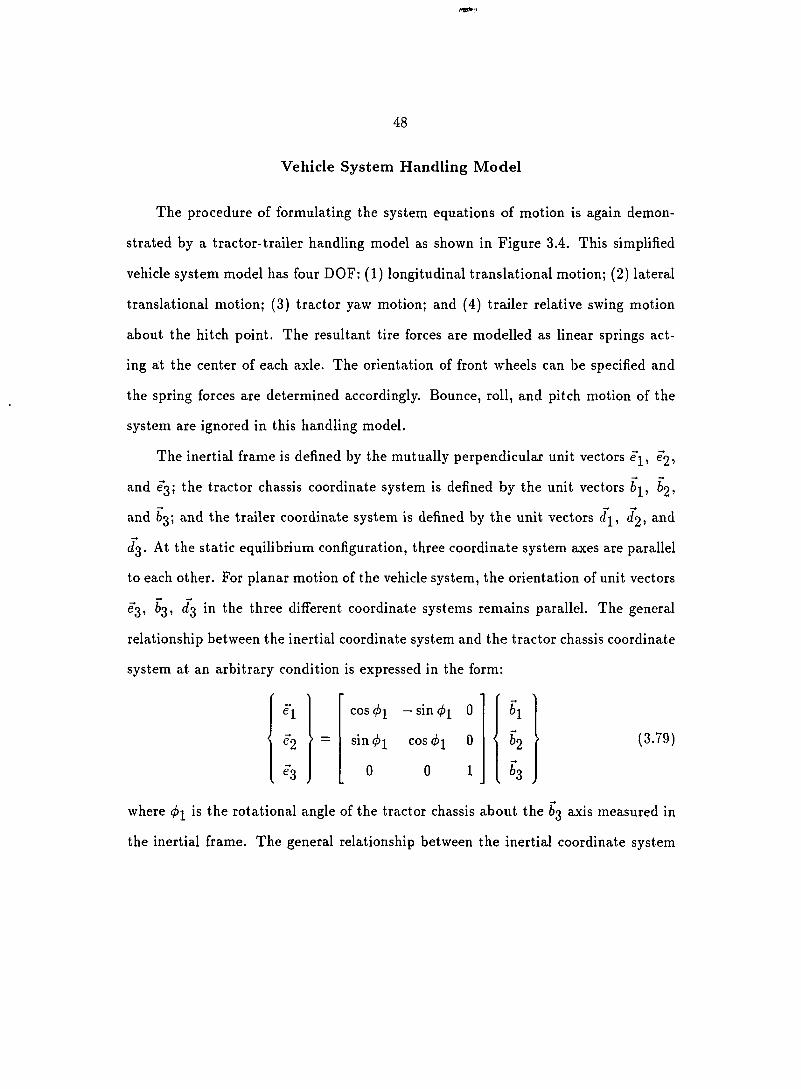
Vehicle System Handling Model 48

Momentum approach 52

D'Alembert's approach 59

Lagrange's approach 61

Hamilton's canonical approach 65

Kane's approach 68

CHAPTER 4. GENERAL-PURPOSE COMPUTER SIMULATION

PROGRAMS 74

CHAPTER 5. SUMMARY 79

BIBLIOGRAPHY 81

APPENDIX A; TRACTOR-TRAILER RIDE VIBRATION MODEL 97

APPENDIX B: TRACTOR-TRAILER HANDLING MODEL .... 100

PART II. FORMULATION OF EQUATIONS OF MOTION FOR

RIGID/FLEXIBLE MULTI-BODY MECHANICAL SYS­

TEMS 103

CHAPTER 1. INTRODUCTION 104

Background and Motivations 104

iv

Literature Review 105

Dynamic principles used to formulate system equations of motion . . 106

Notation selections 107

Modelling of flexible mechanisms 108

Dynamics of closed-loop flexible mechanisms Ill

Dimension reduction of closed-loop mechanisms 114

Objective and Approach 118

CHAPTER 2. GENERAL MODELLING CONCEPTS 120

4 x 4 T r a n s f o r m a t i o n M a t r i x M e t h o d o l o g y 1 2 0

Kinematic Joint Transformation Matrix 123

Rigid Link Shape Matrix 125

Flexible Link Shape Matrix 131

CHAPTER 3. DYNAMICS OF OPEN-LOOP MECHANICAL SYS­

TEMS 137

Kinematic Analysis of Open-Loop Mechanisms 137

Position of a given point 137

Velocity of a given point 138

Acceleration of a given point 142

Generalized Dynamical Equations for Open-Loop Mechanisms 145

System Kinetic Energy Function 146

Kinetic Energy Function Derivatives 149

Derivative of kinetic energy with respect to a joint variable 150

Derivatives of kinetic energy with respect to a modal variable .... 154

System Potential Energy Function 158

V

Potential Energy Function Derivatives 160

System Dynamical Equations for an Open-Loop Mechanism 161

CHAPTER 4. DYNAMICS OF CLOSED-LOOP MECHANICAL

SYSTEMS 163

Kinematic Analysis of Closed-Loop Mechanisms 163

Loop-closure position analysis 164

First partial derivatives of dependent coordinates 177

Second partial derivatives of dependent coordinates 179

Dependent motion computation 182

Velocity of a general point 184

Acceleration of a general point 187

Generalized Dynamical Equations for Closed-Loop Mechanisms 189

System Kinetic Energy Function 192

System Inertia Matrix Derivatives 200

Derivatives of mass matrix with respect to a joint variable 201

Derivatives of mass matrix with respect to a modal variable 202

System Potential Energy and Conservative Forces 204

Non-Conservative System Forces 211

System Dynamical Equation for a Closed-Loop Mechanism 216

CHAPTER 5. SUMMARY 218

BIBLIOGRAPHY 220

vi

PART III. SIMULATION ALGORITHMS AND DEMONSTRATION

EXAMPLES 226

CHAPTER 1. INTRODUCTION 227

CHAPTER 2. SIMULATION ALGORITHM DEVELOPMENT . . 230

Algorithm for Open-Loop Mechanical Systems 230

Inertia coefficients of the system dynamic equation 231

Generalized force vector 237

Algorithm for Closed-Loop Mechanical Systems 240

CHAPTER 3. DEMONSTRATION EXAMPLES 244

Example 1: Double Pendulum Problem 244

Example 2: Mobile Crane Problem 269

Example 3: Front-end Loader Problem 306

CHAPTER 4. SUMMARY 319

BIBLIOGRAPHY 321

GENERAL SUMMARY 323

ACKNOWLEDGEMENTS 325

vii

LIST OF FIGURES

Figures of Part I

Figure 3.1: Tractor-trailer ride vibration model 18

Figure 3.2: Free-body diagram of tractor 23

Figure 3.3: Free-body diagram of trailer 24

Figure 3.4: Tractor-trailer handling model 47

Figure 3.5: Free-body diagram of tractor 53

Figure 3.6: Free-body diagram of trailer 54

Figures of Part II

Figure 2.1: Representation of a position vector 121

Figure 2.2: Kinematic joint j 124

Figure 2.3: Cylindrical joint 126

Figure 2.4: Rigid link shape matrix 127

Figure 2.5: Deformed elastic link 134

Figure 3.1: Representation of an open-loop mechanism 151

Figure 4.1: Representation of spring and damper between two bodies . . 208

Figure 4.2: Spring, damper and forces on a single DOF joint 210

viii

Figure 4.3: Applied body force and torque 212

Figures of Part III

Figure 3.1: Double pendulum (rigid body system) 245

Figure 3.2: Double pendulum (flexible body system) 253

Figure 3.3: Animation of the system (front view) 263

Figure 3.4: Animation of the system (isometric view) 263

Figure 3.5: Driving torque at joint one 264

Figure 3.6: Driving torque at joint two 264

Figure 3.7: Elastic deflection at different configurations 265

Figure 3.8: Animation of system free vibration 266

Figure 3.9: Numerical solution of joint one 267

Figure 3.10: Numerical solution of joint two 267

Figure 3.11: Elastic deflection of point mass mi 268

Figure 3.12: Elastic deflection of point mass 268

Figure 3.13: Mobile crane at work 270

Figure 3.14: Schematic drawing of the crane model 271

Figure 3.15: Definition of local coordinate systems 272

Figure 3.16: Side view of the initial position 276

Figure 3.17: Isometric view of the initial position 277

Figure 3.18: Side view of rear lifting 278

Figure 3.19: Isometric view of rear lifting 279

Figure 3.20: Top view of boom swing motion 280

Figure 3.21: Isometric view of swing motion 281

ix

Figure 3.22: Side view of vertical vibration 282

Figure 3.23: Front view of roll vibration 283

Figure 3.24: Side view of pitch vibration 284

Figure 3.25: Vibrational mode shapes of the boom 285

Figure 3.26: Boom bosition for dynamic analysis 297

Figure 3.27: Elastic deflection of the boom 298

Figure 3.28: Vertical vibration with none and one mode 301

Figure 3.29: Vertical vibration with one, two and three modes 301

Figure 3.30: Roll vibration with none and one mode 302

Figure 3.31: Roll vibration with one, two and three modes 302

Figure 3.32: Pitch vibration with none and one mode 303

Figure 3.33: Pitch vibration with one, two and three modes 303

Figure 3.34: Elastic deflection at first mode 304

Figure 3.35; Elastic deflection at second mode 304

Figure 3.36: Elastic deflection with two modes 305

Figure 3.37: Elastic deflection with three modes 305

Figure 3.38: Ford/New Holland front-end loader system 307

Figure 3.39: Initial position of the linkage 310

Figure 3.40: Rotational motion of the bucket 311

Figure 3.41: Animation of lifting operation 312

Figure 3.42: Animation of chassis horizontal motion 313

Figure 3.43: Animation of bucket dumping motion 314

Figure 3.44: Axial force requirement of tilting cylinder 315

Figure 3.45: Axial force requirement of lifting cylinder 316

X

Figure 3.46: Initial position of the lifting system 317

Figure 3.47: Deflection of lifting system at lower position 317

Figure 3.48: Deflection of lifting system at middle position 318

Figure 3.49: Deflection of lifting system at upper position 318

xi

LIST OF TABLES

Table of Part I

Table 4.1: Multibody simulation software packages 76

Tables of Part III

Table 3.1: Properties of the system 260

Table 3.2: Parameters of the mobile crane 295

1

GENERAL INTRODUCTION

Introductory Comments

Dynamic analysis of mechanical systems plays an important role in optimum

design and automatic control of such systems. Computer simulation has become an

indispensable tool used to predict motion response and to optimize performance of

complex vehicles and machinery. Different mechanics methods have been employed to

develop computational algorithms to provide the theoretical background for general

purpose computer simulation programs. The evaluation of relative advantages of each

method of formulating the system equations of motion provides a general guidance

for improving or developing sophisticated computer simulation programs.

One of the goals of advanced design of mechanical systems is to reduce the pro­

duction cost by reducing the size and modifying the physical dimensions with the

performance quality maintained. The effects of linkage flexibility on the dynamic

performance of a mechanical system need to be considered for high quality design

and accurate control. The large displacement motion of a mechanical system with

flexibility effects from its members has distinguished the problem from either pure

rigid-body dynamic analysis of the system as the traditional mechanical engineering

approach, or the pure elastic deflection analysis of the structure as the traditional

2

structural engineering approach. It is desirable to have a general unified computa­

tional methodology to analyze the dynamic behavior of mechanical systems having

large displacement motion with flexibility effects of their members.

The objective of this research is to develop a general computational methodol­

ogy for dynamic analysis of multi-link, geometrically-constrained, rigid/flexible me­

chanical systems. To achieve this goal, a review of theoretical mechanics methods

was conducted and evaluated by considering the tractor-trailer system handling and

ride vibration problems. A unified 4x4 transformation matrix approach has been

employed to develop the simulation algorithm. As a demonstration of applying the

algorithm, three simplified examples were used to show the open-loop and closed-loop

mechanical systems.

Outline of Dissertation

This dissertation consists of three parts in technical paper format. Part I

(Computer-oriented analytical dynamics for machinery and vehicle systems) focuses

on the dynamic principles and applications to tractor-trailer systems. Part II (Formu­

lations of equations of motion for rigid/flexible multi-link mechanical systems) covers

the basic modeling concepts and the development of system equations of motion using

4x4 transformation matrix approach. Part III (Simulation algorithm and demon­

stration examples) deals with the algorithm development and the demonstration of

using the algorithm to model selected mechanical systems.

Part I presents an overview on five mechanical principles used to formulate sys­

tem equations of motion, namely. Momentum principle, d'Alembert's principle, La­

grange's equation, Hamilton Canonical equation and Kane's equation. The relative

3

advantages of each method were evaluated by considering a tractor-trailer ride vi­

bration and handling model. Contemporary general-purpose computer simulation

programs for analyzing mechanical systems based on one of the five methods were

summarized at the end of the part with related literature references.

Part II develops a general modeling concept for both rigid and flexible mechanical

systems with the 4x4 transformation matrix approach. The kinematics of the system

were determined from the geometric constraint equations. An open-loop mechanical

system was modelled by considering both the large-displacement geometric constraint

variables and elastic modal variables. Closed-loop mechanical systems were modelled

by determining the degrees of freedom from system geometric constraint equations

and setting up dynamic equations based on the number of system degrees of freedom.

Part III presents an algorithm for formulating system equations of motion. As

a demonstration, a flexible double pendulum was modelled as an open loop system.

The elastic deflection was estimated by using assumed mode shape functions. The

equations of motion were formulated with a step-by-step procedure and were numer­

ically integrated from given initial values. The second example dealt with a mobile

crane system. The chassis was modelled as a rigid body supported by flexible out­

riggers. The vibrational motion of chassis was analyzed by considering the flexibility

efl'ects of the boom. Computer simulation was conducted based on estimated system

parameters. The third example discussed a front-end loader with flexible linkage.

The linkage was modelled as closed-loop mechanical systems. Elastic deflection at

diflferent operational configurations was computed.

4

PART I.

COMPUTER-ORIENTED ANALYTICAL DYNAMICS FOR

MACHINERY AND VEHICLE SYSTEMS

5

CHAPTER 1. INTRODUCTION

Principles of Mechanical Dynamics

Simulation methodologies to predict motion response and optimize performance

of complex vehicles and machinery are receiving greater attention. Numerous analyt­

ical mechanics methods are employed to produce computational algorithms to predict

vehicle and machinery dynamic response by means of numerical solutions of initial-

value problems. The relative advantages of each method to formulate the equations

of motion are evaluated in terms of the effort required for the formulation and the

simplicity of the equations' final form. For complex mechanical systems, excessive

computer storage limitations and execution time may cause problems if the equations

are not expressed in the simplest form. On the other hand, the effort required to

formulate the equations in their simplest form may be prohibitive unless an efficient

methodology is used at the outset. For relatively simple problems, neither criterion

is important [1-3].

Engineering mechanics consists of a study of both statics and dynamics of rigid

and flexible bodies. Statics deals with the force equilibrium of bodies in a system at

rest or moving with constant velocity. Dynamics deals with bodies having accelerated

motion and is subdivided into two subjects: (1) kinematics which deals with the

geometrical aspects of motion and (2) kinetics which deals with the analysis of forces

6

causing the motion. Mechanical systems are comprised of links interconnected in such

a way that specified input forces and motions are transformed to produce desired

output motions and forces. The relationship between the motion of a system and

the forces acting on it is governed by the equations of motion and the geometric

constraint equations. From known applied forces, the motion can be predicted from

the system equations. When the desired motion is specified, the required driving

forces are computed from the equations of motion.

To formulate the dynamical equations for vehicles and machinery, the design

analyst may either construct the literal system equations of motion by hand or use 'so-

called' multibody simulation programs which automatically formulate the equations

of motion numerically or symbolically. These programs are applicable to solve a wide

class of problems by means of a structured program input procedure. Sometimes, a

given multibody program is not applicable to a particular problem. Thus, the analyst

is forced to make program additions and modifications in order to eliminate inefficient

and inaccurate simulations. Moreover, the procedures for the formulation of literal

equations of motion furnish the basis for a multibody program which reduces the

computer storage requirements and execution time.

Both the Newton-Euler and Lagrangian methods have been widely used in study­

ing the dynamics of multibody mechanical systems (e.g., mechanisms, robots, ground

and space vehicles) and have been well documented in references [4-19].

One application of multibody dynamics methodologies is the design analysis of

aerospace vehicles. Because these systems have free motion in space as compared

to the mechanisms which are always connected to an inertial frame, the traditional

dynamic principles are difficult to use because of the complicated coordinate system

7

conversions. Based on the Lagrangian formulation and the D'Alembert's principle,

another formulation procedure-called Kane's method-was developed in 1960s. This

method starts with the definition of the generalized speeds. The partial angular ve­

locities and partial translational velocities can be expressed in terms of the system

configuration and the generalized speeds. The general active and inertial forces are

determined by using vector dot-product operations. The summations of the active

and inertial forces corresponding to each of the independent variables produce the

scalar equations of motion for the system [20-22]. The application of Kane's method

has simplified the procedure of formulating the system equations of motion for space

structures and open-loop mechanisms [23-43]. Two approaches are used to model

closed-loop mechanical systems. In the first approach, the system equations of mo­

tion are derived by selecting the independent variables and using the loop closure

equations. In the second approach, the system is first broken into an open-loop sys­

tem at a selected joint and the equations of motion for the open loop system are

derived. The undetermined lagrangian multipliers are used to impose the system

geometric constraints [44-54].

Significant research has been conducted on the modelling and simulation of open-

loop mechanical systems (i.e., robots, vehicles). The articulated-body-inertia method

has been developed to formulate the system equations of motion recursively [55-56].

The basic idea is that the method allows the assemblage of geometrically constrained

bodies which make up the articulated mechanism to be treated as a single-rigid-

body-like element of the system. This method is most efficient for handling open-

loop kinematic chains, but is very inefficient in handling closed-loop kinematic chain

mechanisms [57-63].

8

Another application of multibody dynamics methodologies is the study of ground

vehicle systems. The Newton-Euler method requires the development of a free-body

diagram for each component [64-70]. This approach needs to introduce the internal

forces at each geometrical constraint point and subsequently eliminates these forces

to obtain the system equations of motion. Lagrange's method is also used to formu­

late the dynamic equations of motion for vehicle systems [71]. This approach allows

relative coordinates to be used in describing the system configuration. The derivative

operations require the absolute quantities to be expressed in terms of these coordi­

nates and the computations may be difficult to perform. Kane's method has been

found easier to use in formulating the system equations of motion for vehicle systems

when compared to Newton-Euler or Lagrange's method [72-73].

The relationship between different body coordinate systems is represented by

the geometrical transformation matrix. Euler angles are commonly used to define

body orientations. When the uncertainty of system configurations may cause system

transformation matrix singularities, Euler parameters are used in some studies to

represent the relationship between different coordinate systems [74-78].

Objective and Scope

To support the conclusions that the formulation method which provides the

equations of motion with the least effort and in the simplest form should be the

basis for a multibody program, the theoretical principles for multibody dynamics are

reviewed. Five methods are addressed, namely, the use of momentum principle or

the Newton-Euler method, D'Alembert's principle, Lagrange's method, Hamilton's

Canonical method, and Kane's method. The first two methods are classified as vector

9

dynamics approaches while the third and fourth methods are classified as analytical

dynamics approaches (or energy methods in dynamics). The last method, sometimes

called Lagrange's form of D'Alembert's principle, is considered as a hybrid of the

vector and analytical dynamics approaches.

The system equations of motion for tractor-trailer ride vibration and handling

problems are derived by using each of the five approaches. The procedures for five

different methods are compared in terms of simplicity in the formulation process.

With system geometry, inertial, damping, and stiffness properties of a tractor-trailer

system, the natural frequencies and vibrational mode shapes may be obtained from

these system equations. The system time domain response is obtained numerically

by integrating these equations for specified initial values.

The state-of-art in the field of modeling and simulation of multibody mechanical

systems is presented at the end of the section by a comprehensive summary of general-

purpose computer simulation programs based on these dynamics principles.

10

CHAPTER 2. THEORETICAL BACKGROUND OF DYNAMIC

PRINCIPLES

Momentum Principle

The momentum principle relates the acceleration of a body to the forces acting

on it in vector form. Any mechanical system composed of multiple bodies must be

separated and represented by a series of free body diagrams which show all internal

and external forces acting on each isolated body. The translational equations of

motion for a body are written in the general form:

| ( i ) = f ( 2 - 1 )

where L = mKc is the linear momentum of the body; V Q is the velocity vector

at the mass center C; F is the resultant external force acting on the body which

includes applied forces and geometrical constraint forces resulting from the separation

of adjacent bodies. The rotational equations of motion for a body are written in the

general form:

— ( ^ c ) • T c ( 2 . 2 )

where H e = / r x (w x f ) d m is the angular momentum about the mass center of the

body; r is the position vector of the mass particle dm from the mass center; Tc is the

r e s u l t a n t m o m e n t o f e x t e r n a l f o r c e s a n d c o u p l e s a c t i n g a b o u t t h e m a s s c e n t e r C .

11

The momentum principle provides a straight forward and meaningful procedure

to obtain the equations of motion for an individual body. The introduction and

subsequent elimination of internal forces at the geometrical constraints, however,

make it difficult to formulate the equations of motion for the system. The angular

momentum principle requires location of the mass center of the body to which the

principle is being applied.

After introducing the so-called 'inertial forces', D'Alembert proposed a principle

which states that the applied active forces together with inertial forces form a system

in equilibrium. The problem in dynamics, therefore, could be reduced to an equivalent

one in statics. For an individual body, the translational inertial force is defined as:

where m is the mass of the body; dc is the acceleration at the mass center. The

rotational inertial torque is defined as:

where I is the central inertial dyadic of the body; a and w are the angular acceleration

vector and the angular velocity vector, respectively. The translational equation of

motion for the body can be written as:

D'Alembert's Principle

F = — mac (2.3)

f * = - ( I - a + w X ( I - w ) ) (2.4)

F + F* = 0 (2.5)

and the rotational equation of motion for the body can be written as:

f + f * = 0 (2.6)

12

where F and T are the applied resultant forces and torques on the body, respectively.

D'Alembert's principle, which produces the equations of motion in vector form

as with the momentum principle, allows the dynamical problem to be treated as

an equivalent static one. Any convenient point can be used as a reference point to

determine the dynamic torque equilibrium equation. With the momentum principle

the mass center is the only point that may be used to develop rotational equations

of motion. Because the principle is developed for an individual body, rather than

for the system, the introduction and subsequent elimination of internal forces at geo­

metric constraint points make it difficult to develop the system equations of motion,

particularly for large degree-of-freedom (DOF) systems.

By using generalized coordinates rather than physical coordinates, Lagrange for­

mulated dynamical equations of motion from the kinetic energy and potential energy

expressions, which are scalar quantities and can be manipulated in an arithmetic

manner. The system of bodies is considered as a whole instead of being separated

into individual components. The constraint forces that do not perform work are

not included in the energy equation. The minimum number of equations of motion

directly corresponds to the independent generalized variables.

For a holonomic n DOF system, q i , 52» • • • • > I n are the independent variables.

The equation of motion corresponding to each independent variable is written in the

general form;

where L = T — V '\s the Lagrangian; T and V are system kinetic and potential

Lagrange's Method

13

energies, respectively; is the nonconservative generalized force corresponding to

the virtual displacement ôq^.

Lagrange's method makes use of the kinetic and potential energies. A multibody

system can be considered as an entity. The minimum number of independent equa­

tions of motion are formulated corresponding to each independent variable. For a

nonholonomic system, not all the generalized variables are independent. Lagrangian

multipliers must be used to determine the geometrical constraint forces. The proce­

dure requires the partial derivative and total time derivative of the energy functions.

The formulation may be complicated and time consuming; therefore, more effort is

needed in formulating the equations of motion for large DOF systems.

The system equations of motion can be expressed as a set of 2n first-order equa­

tions by choosing generalized coordinates and generalized velocities as the state vari­

ables. Hamilton's canonical equations use the generalized coordinates and generalized

momenta as state variables for setting up the dynamical system equations.

For a dynamic system, n generalized momenta are defined as:

where L = T — V is the Lagrangian function. The potential energy function, V, is

not velocity dependent; therefore, the derivative of V with respect to is zero.

A scalar Hamiltonian function is defined as:

n

Hamilton's Canonical Method

(2.8)

H = Y , v m - (2.9) i=l

14

Under the condition defined by Equation 2.8, the first part in the Hamiltonian func­

tion can be related to the system kinetic energy in the form:

E Piii = 2T (2.10) 1=1

Therefore, the Hamiltonian function can be rewritten as:

H = 2 T - L = 2 T - { T - V ) ^ T + V (2.11)

Equation 2.11 shows the Hamiltonian function to be the total energy function of the

system. The relationship between q.^ and is determined after using Equation 2.8.

The Hamiltonian function is then expressed in the form:

H = H ( q i , 9 2 , • • • ) P i , P 2 ' P n , 0 ( 2 . 1 2 )

Then a set of '2n first-order equations can be written as:

d H = %

i i = i = l , 2 , . . . , n ( 2 . 1 3 )

The solution of = /(g^, g'g, ..., q n ) is not easily obtained analytically because

it involves the inversion of n x n mass matrix. The difficulty can be overcome by

working with implicit energy functions and numerically evaluating the relationship

at a given instant of time. When a numerical solution package requires a set of first-

order differential equations, the generalized coordinates and generalized velocities are

often chosen as the state variables. These first-order equations may be determined

from the second-order system equations formulated by any of the other analytical

methods.

15

Kane's Method

Kane's method may be applied to any system whose configuration in a Newto­

nian reference frame is specified by n generalized coordinates gj, 52> --, This

method involves two sets of quantities, namely, the partial angular velocities and the

partial velocities. If the variables, ug; •••, called the 'generalized speeds',

are introduced as the linear combination of the time derivative of the generalized

coordinates in the form:

n + X;, i = l,2, . . . , 7 î (2.14)

j = l

where W ^j and A'j are functions of q 2 , ••., q n and time t . If W ^j and { i , j =

1 , 2 , . . . , n ) a r e c h o s e n s u c h t h a t E q u a t i o n 2 . 1 4 c a n b e s o l v e d u n i q u e l y f o r q ' o , . . . , q n ,

the angular velocity of any body and the velocity of any point can be uniquely ex­

pressed as a linear function of U2,..., un- The vector that is the coefficient of

lij in such a function is called the ith partial angular velocity of the body, or the it h

partial velocity of the point.

The equation of motion corresponding to each independent is formulated in

the form:

A'j + A'* = 0, (i = l,2,...,n) (2.15)

where ATj is the ith generalized active force; A'* is the ith generalized inertial force.

For an n DOF system, the ith generalized active force is computed in the form:

N h . (2 .16)

J = 1

where Nf^ is the total number of bodies in the system; and ujj are the partial

velocity vector and partial angular velocity vector of body j with respect to the

16

generalized speed Wj, respectively; F j and T j are the applied resultant forces and

torques at body j, respectively. The partial velocity vector is computed from the

velocity vector at the point where the force Fj is applied in the form:

... ay.

= A I

The partial angular velocity vector is computed from the angular velocity vector of

body j in the form: ? aw;

The ith generalized inertial force A'* is computed in the form;

% . Ki = EiV/ -Fj+^^l-fj) (2.19)

J = 1

where and wj are the ith partial velocity vector at the mass center and the ith

partial angular velocity vector of body j, respectively; Fj and Tj are the inertial

force and torque on body j, which are computed in the same way as for D'Alembert's

principle.

Kane's equation requires the least effort to formulate the system equations of

motion when compared to the classical methods. The system is considered as a unit.

Non working forces at the geometrical constraint points are not included, therefore,

the elimination of internal forces as required by Newton-Euler and D'Alembert's

methods is eliminated. The vector dot product operation is used to obtain the scalar

equations. The derivative operations of the kinetic and potential energy functions,

which may be difficult to obtain, are also eliminated.

17

CHAPTER 3. TRACTOR-TRAILER SYSTEM MODELS

Ride Vibration Model

The five dynamics principles provide the basis for formulating the system equa­

tions of motion. Procedures for using each of the five methods are demonstrated by

considering a tractor-trailer ride vibration model in this section, and a tractor-trailer

handling model in the next section

Figure 3.1 is a representative diagram of a tractor-trailer ride-vibration model.

The planar model has four DGF: (1) tractor bounce motion; (2) tractor pitch motion;

(3) tractor longitudinal motion; and (4) tractor-trailer relative pitch motion. It is

assumed that the tires are modelled by linear springs and that they are the only

suspension elements inasmuch as the tractor and trailer bodies are rigid and have no

wheel suspension. Lateral, roll, and yaw motions are ignored in this simplified model.

It is noted that the inertial reference frame is defined by the unit vectors ei, eg, and

60, while the tractor chassis coordinate system is defined by the vectors 6]^, bg, and

63, and the trailer coordinate system is defined by the vectors di, and d^. It is

also noted that the general angular orientation of tractor chassis coordinate system is

measured by while the general angular orientation of trailer coordinate system

is measured by (0]^ -t- #2)^2- The general relationship between the inertial reference

Figure 3.1: Tractor-trailer ride vibration model

19

system and the tractor chassis coordinate system is expressed in matrix form as:

h

h

. '3 .

«2

. ^3 .

COS#! 0 sin

0 10 62 ' (3.1)

— sin 9-1 0 cos Oi

The general relationship between the inertial reference system and the trailer body

coordinate system is expressed in matrix form as:

cos(#2 + #2) 0 sin(0]^ + #2) ^1

0 1 0 (3.2)

— sin(#2 + #2) 0 cos(0]^+#2) ^3

At the static equilibrium position, 6^ and 62 are equal to zero, and the three coordi­

nate system axes are parallel to each other.

The position vector from the origin of the inertial reference frame to the center

of gravity of tractor chassis (i.e., origin of the tractor chassis coordinate system) is

expressed in the form:

Rl = xe-^ + zeg (3.3)

where x and z are the horizontal and vertical displacements measured in the global

frame, respectively. The position vector to the center of gravity of trailer (i.e., origin

of the trailer coordinate system) is expressed in the form:

•^2 ~ -^1 ~ (^1 + -^3)^1 + (-^8 "t" ^6)^3 " -^4^1 — ^ 7 ^ ^ (3.4)

where and X3 are the horizontal distances from the rear axle to the tractor center

of gravity and the hitch point, respectively; Xg and LQ are the vertical distances from

the tractor rear axle to the tractor center of gravity and the hitch point, respectively;

20

and L'j are the horizontal and vertical distances from the trailer center of gravity

to the hitch point, respectively.

The absolute translational velocity of the tractor chassis is expressed in the form:

VY — xei + zeg (3.5)

while the absolute angular velocity of the tractor chassis is expressed in the form:

^1 = h^2 (3.6)

The angular velocity of the trailer is expressed in the form:

(3 .T)

while the translational velocity of the trailer is expressed in the form;

9-2 = xei + ((LQ + LQ)éi)bi - {Ljièi + ê2))di

+ iêg + ((Li + £3)01)63 + (X4(0i + 02))'^3 (3.8)

When expressed in global coordinate system, Equation 3.8 can be written as:

V 2 = + JD3)sin01 + 0]^(Zg + Ig)cos0]^

+(^1 + 2) [-^4 sin(0]^ + O 2 ) — L j cos(02 + ^2)]}

+ + L^) cos 9-^ — -|- Zg) sin 9-^

+(^1 + 2) [-^7 sin(0j + ^2) + -^4 cos(02 + ^2)1} (3.9)

The translational acceleration of the tractor is expressed in the form:

di = xei + 263 (3.10)

21

while the angular acceleration of the tractor chassis is expressed in the form:

ai = g'leg (3.11)

The angular acceleration of the trailer is expressed in the form:

a.2 = 0 1 + 6 2 ) 6 2 (3.12)

while the translational acceleration of the trailer is expressed in the global coordinate

system in the form:

®2 — + X3) sin^l + 0^(L^ + £3) cos

"^^1(^6 ^1 ~ 4- Lg)sin9-^

+•^4(^1 + ^2) sin(^2 + ^2) ^4(^1 "I" ^2)^ cos(^2 + ^2)

— L ' j { 9 - ^ + ^2) cos(^2 + 2) + -^7(^1 + ^2)^ sin(0j + #2)}

+ + ^'l(-^l 4" X3)cos0]^ — )sin

-^l(Ig + L ^ ) s m 9 i - 9 i { L Q + Ig)cos#i

-\-Lj^ ( 9 - ^ 4 - ^ 2 ) c o s ( ^ 2 4 " ^ 2 ) ~ - ^ 4 ( ^ 1 4 - 2 s i n ( 4 - 2 )

+ + §2) sin(^2 4" ^2) 4- -^7(^1 4- ^2)^ cos(^j^ 4- ^2 )} (3.13)

At the static equilibrium configuration (i.e, = ^2 ~ 0), the absolute transla­

tional acceleration of the trailer can be simplified as:

"2 — ^l{^ 4-^|(Zi 4-Z3) 4-^1(^6 4-Zg)

+ L^(9i + ^2)^ - -^7(^1 4- ^2)}

4- e ^ { z + 9 i ( L i + L ^ ) - 9 ^ ( L g + L g )

4-14(^1 4- ^2) 4- Zy(^2 + ^2)^} (3-14)

22

The external force applied at the tractor front axle is expressed in the form:

F j = —A'yr^{a; + £2(^05^1 — 1) + Zg sin^j^jej

—Kj^{z — L2 sin d-^ + Zg(cos 9^ — l)}eg (3.15)

where Kand Kare the tractor front tire equivalent stiffness in vertical and

horizontal directions, respectively; L2 and Xg are the horizontal and vertical distances

from tractor center of gravity to front axle center line, respectively. The external force

applied at the rear tractor axle is expressed in the form;

F'P = —Ktx{X + Zig sin (cos 9-^ — 1

— 4- Z/g(cos0| — 1) 4- sin(.3.16)

where Krz and Krx are the tractor rear tire equivalent stiffness in vertical and

horizontal directions, respectively.

The external forces applied at the trailer wheel is expressed in the form:

Fs = —Ks{z + (Zfg + Zg)(cos — 1) + (Li + Zg ) sin

+ (Zr4 + Z5)sin(^i + ^2) + (-^10 ~ ^2) ~ ^)}^3 (3.IT)

where Ks is the vertical equivalent stiffness of the trailer tire; and are the

horizontal and vertical distances from trailer center of gravity to trailer axle center

line, respectively.

The weights of the tractor and trailer are balanced by the initial tire deflection

and do not enter the system equations of motion for tractor-trailer ride vibration

model which are developed through five different methods in following subsections.

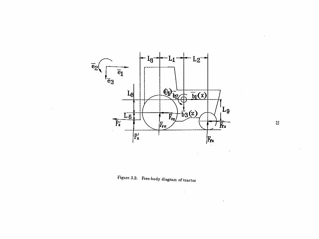
to

Figure 3.2: Free-body diagram of tractor

I 63

to

Figure 3.3: Free-body diagram of trailer

25

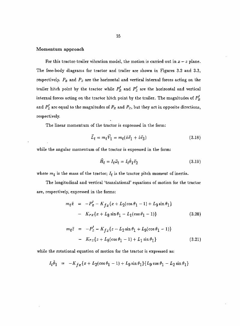
Momentum approach

For this tractor-trailer vibration model, the motion is carried out in z — z plane.

The free-body diagrams for tractor and trailer are shown in Figures 3.2 and 3.3,

respectively. Px and Pz are the horizontal and vertical internal forces acting on the

trailer hitch point by the tractor while P^ and Pl are the horizontal and vertical

internal forces acting on the tractor hitch point by the trailer. The magnitudes of

and P~ are equal to the magnitudes of Px and Pz, but they act in opposite directions,

respectively.

The linear momentum of the tractor is expressed in the form:

+ zeg) (3.18)

while the angular momentum of the tractor is expressed in the form:

Ht = = hhh (3.19)

where is the mass of the tractor; is the tractor pitch moment of inertia.

The longitudinal and vertical 'translational' equations of motion for the tractor

are, respectively, expressed in the forms;

mix = — Pj — 0;!^ — 1)-i-Lg sin^^}

— I^rx{^ 4" Zig sin ^2^ — //^(cos ~ 1 )} (3.20)

mi'z = — pl — K j:^{z — L2 sin 6-^ + Lglcosdi — 1)}

— K r z { ~ 4- irg(cos — 1) -f L - ^ sin} (3.21)

while the rotational equation of motion for the tractor is expressed as:

+ ^2(^0® 1 ~ 1) + ^9 cos — ^2

26

- Krx{x + Lq sin - Li{cosOi - l)}{Zg cos#i + sin ^2}

+ Kj^{z — f 2 sin di + Zg(cos 9i — l)}{i^2 ^1 + -^9 ^ll

- Krz{^ + L^{cos9i - 1) + sin0]^}{Z^ cos#i - Igsin^j^}

~ -Pz{(^6 + Zg)sin^2}

- + - ^ 3 ) ^ ° ® ^ ! ~ ( - ^ 6 + ( 3 . 2 2 )

The linear momentum of the trailer is written in the form:

Ls = rngV^ (3.23)

where V2 is the velocity vector at trailer mass center as shown in Equation 3.9 while

the angular momentum of the trailer is expressed in the form:

Hs = l3<^2 - s0i + ^2)^2 (3.24)

where rus is the mass of the trailer; Is is the trailer pitch moment of inertia about

the mass center of the trailer.

The longitudinal and vertical translational equations of motion for the trailer

are, respectively, expressed in the forms:

+ (Z)^ + L^)(6i sin 6^ + 6^ cos di )

+ ( L Q + L G ) { 6 I COS#! ~ sin#]^) + sin(#2 + 9 2 ) ( L ^ { 0 I + O 2 )

+-^7(^1 + 2)^) + cos(0j + 92){L^{èi + 6^)2 - Lj{9i + #2))} = Px (3.25)

+ {Li + L^)(9i cos#i - sin #2)

- { L q + L g ) ( 9 i sin#! + cos#j) + sin(#i + #2)(^7(^1 + 2)

- L ^ I È I + 6^)2) + cos(#i + 9 2 ) ( L ^ { 9 I + #2) + ^7(^1 + 2)^)}

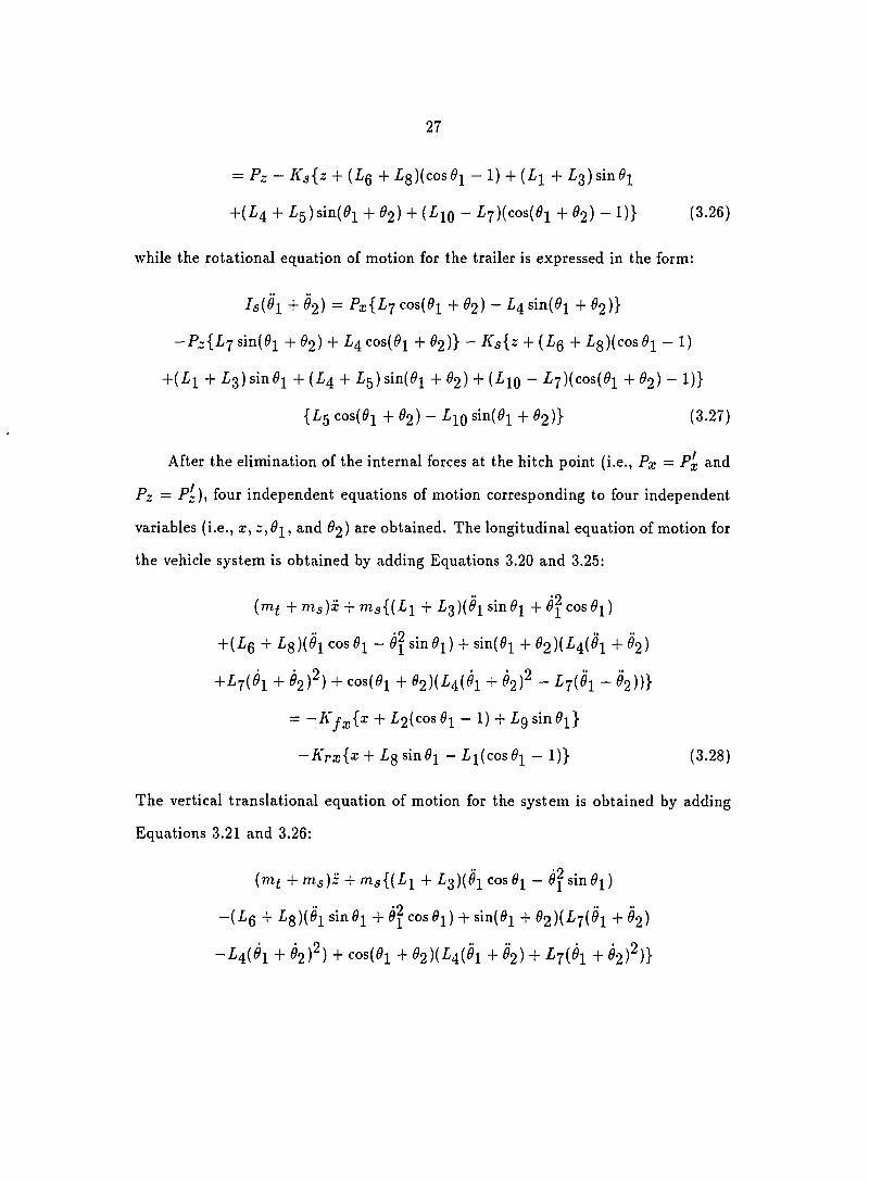
27

— P z ~ + (//0 + i/g)(cos— 1) + (X]^+ Z13)sin

+{L^ + ig)sin(^2 + 2) + (-^10 ~ LY)(cos{OI + ^2) ~ ^)} (3.26)

while the rotational equation of motion for the trailer is expressed in the form:

+ ^2) — P x { L i cos(^2 4- 6 2 ) - •t'4 sin(0]^ + #2)}

— P z { L ' j sin(0j + 2) 4" -^4 cos(^2 + ^2)} ~ + {L Q + ig)(cos — 1)

+(^1 + ) sin + (X4 + Zrg) sin(0j + 2) (^10 " £7)(cos(0]^ + ^2) " 1)}

{Zf5 cos(^^ + ^2) — ^10 sin(0j + #2)} (3.27)

After the elimination of the internal forces at the hitch point (i.e., P x = P x and

Pz = P-), four independent equations of motion corresponding to four independent

variables (i.e., x, and 62) are obtained. The longitudinal equation of motion for

the vehicle system is obtained by adding Equations 3.20 and 3.25:

(m^ + ms)x + ms{{Li + L^){6i sin^j + cos#i)

+(ig + iyg)(^'j^ COS 9 ^ — 0 ^ s i n ) 4 - s i n (^2 4- ^2)(^4(^1 4" ^2)

+Lf{di + ^2)^) 4- cos(^j 4- 02)(-^4(^1 4- 6^)^ — 1^01 + ^2))}

= —Kfx{^ 4- L2{cos — 1) + Lg sin^j^}

— Kfxi^x + Lg sin ~ Z]^(cos — 1)} (3.28)

The vertical translational equation of motion for the system is obtained by adding

Equations 3.21 and 3.26:

(m^ + ms)z 4- ms{{Li + Zg)(^2 cos#i - 0^ sin )

-(Ig + lg)(0i sin0j + 9 ^ cos g^) + sin(^2 + ^2)(-^7(^l 4- ^2)

— L^{§i + 6^)2) + cos(0]^ 4- ^2)(^4(^1 4- ^2) 4- 4- ^2)^)}

28

= —KjJ^z — L2 sin + Lg(cos 6^ ~ 1)}

— 4 " Z g ( c o s d - ^ — 1 ) 4 - L - ^ s i n 6 - ^ }

—Aj{z 4- (Zrg + L^){cos6i — 1) + {Li + i^g)sin^2

+(L^ + L^)sin{9i + 62) + {LIQ - Z%)(cos(^2 + ^2) ~ 1)} (3.29)

The pitch motion of the system about tractor center of gravity is obtained by adding

Equations 3.22 and 3.27 and using Equations 3.25 and 3.26 to replace the internal

forces:

Il6i + Isi^i + 2) + + (^1 + L^){6i sin 9^ + cos 6^ )

+(^g + LQcos 2 — 9^ sin+ sin(^2 + 2+ 2)

+£7( ^ 1 + 6 ^)2) + cos(0]^ + ^2)(j^4(^l + 2)^ - L-j{9I + #2))}

{ ( L Q + Zg)cos#i 4- { L I + Zg) sin^2 - cos(^2 + ^2)

+ sin(^2 + #2)} + Tnsi'z + (ij 4- L^){9i cos#i — 9^ sin^2)

—{LQ + sin 9-^ •\- 9^ cos ) + sin(0j^ + ^2)(^7(^l 4- <^2)

-^4(^1 + ^2)^) + cos(0j 4- ^2)(^4(^1 + ^2) + ^7(^1 + #2)^)}

{(L]^ 4" Zfg) cos 9-^ — (Zg 4" Zfg) sin4- Lj sin(0j 4" ^2) -^4 cos(4- 2)}

= —Kyg.{z 4- L2{cos 9-^ — 1) 4- X9 sin 9i}{Lg cos 9i — L2 sin^|}

—Krx{^ + ^g sin 9^ — Li{cos 9-^ — l)}{ig cos 9i + Li sin 2}

+Kj:^{z — L2 sin4- Zg(cos cos 9i 4- Zg sin^j}

—Krz{z 4- Ig(cos — 1) 4- sin 9i}{Li cos 9i — Lg sin 0]^}

— Ks{z 4" {LQ + Zg)(cos 9-^ — 1) 4- 4- Zg) sin9^ 4- {L^ 4- -£5) sin(0]^ 4- ^2)

+(•^'10 ~ -f'7)(cos(0]^ 4- ^2) ~ 1)}{(-^1 + 3) cps#i — {LQ 4- I'g)sin0]^

+(^4 + 5)cos(^l + h) ~ (^^0 - L'j)sm{9i 4- #2)} (3.30)

29

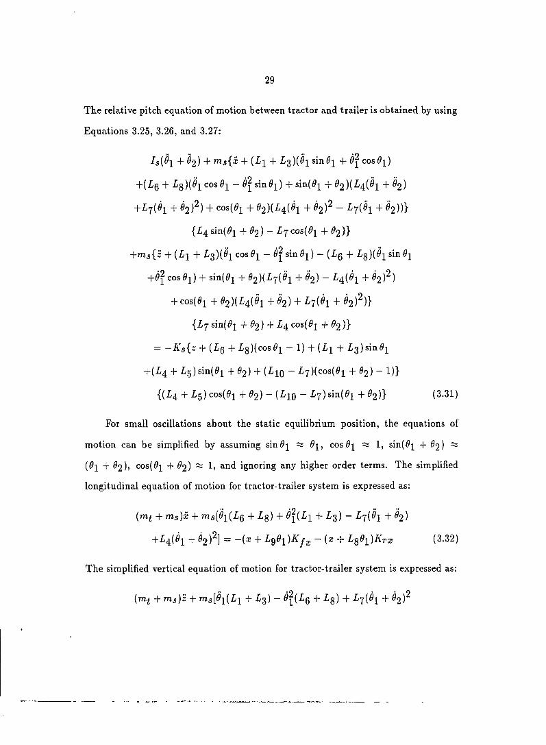
The relative pitch equation of motion between tractor and trailer is obtained by using

Equations 3.25, 3.26, and 3.27:

+ 2) 4- { L - ^ + sincos9 - ^ )

-\-{LQ + L Q ) { 9 I cos 9 I - 9 ^ sin^2) + sin(0]^ + 2)(-^4(^"l + ^2)

+£7(^1 + 6^)2) + cos(^2 + ^2)(-^4(^l + ^2)^ ~ ^701 + ^2))}

{Z4, sin(^2 + 02) ~ ^7 cos(^l + ^2)}

+ms{z + (^1 + L ^ ) { 9 I C O S 9 I - 9 ^ sin^j) - [ L Q + sin^^

+^2 cos#i) + sin(^2 + 9 2 ) { L ' j [ 9 I + 2) - -^4(^1 +

+ cos(^2 + ^2)(^4(^1 + ^2) + -^7(^1 + ^2)^)}

{Z7 sin(^2 + ^2 ) + -^4 cos(^l + ^2 )}

= -A's{z + [L Q + LQ){cos9I -1)4- {Li + i3)sin0]^

+(L^ + Zr5)sin(02^ + ^2) + (-^10 ~ -£'7)(cos(^^ + ^2) ~ 1)}

{(^4 + 5) cos(^2 + ^2) ~ (•^'10 ~ £7) sin(0j^ + ^2)} (3.31)

For small oscillations about the static equilibrium position, the equations of

motion can be simplified by assuming sin^^ ~ cos #2 % 1, sin(0]^ + ^2) ~

(0]^ + #2), cos(^2 + ^2) ~ 1) and ignoring any higher order terms. The simplified

longitudinal equation of motion for tractor-trailer system is expressed as:

{mi + ms)x + ms[6i{LQ + Zg) + + £3) - -£7(^1 + ^2)

+ ^2)^] ~ 4- Lg9-^)K— (a: 4" L^9-^)Krx (3.32)

The simplified vertical equation of motion for tractor-trailer system is expressed as:

( m f - 4- T n s ) z 4- 4- X3) — 9 ' ^ { L q 4- Xg) 4- 4- 6^)^

30

+^4(^1 + 2)1 ~ •^/z(-^2^1 ~ -^rz(z 4- -^i^l)

—Ks{z + {Li + £3)^1 + (i/4 + L^){Oi + #2)) (3.33)

The simplified pitch equation of motion corresponding to is expressed as:

h ^ l + - ^ 5 ( ^ 1 + 2 ) ( ^ 6 + - ^ 8 L ' j ) T n s [ x + [ L ^ + L ^ ) 9 ^

+ { L q + L ^ ) $ i — L j i O i + O 2 ) + L ^ { ê i + 2 ) ^ 1 + ( ^ 1 + - ^ 3 + L / ^ ) m s [ z

+{LI + — {LQ + LG)È^ + £7(^1 + 2)'^ + -^'4(^1 + ^"2)1

- + 9 ^ l ) A f x ~ + L Q 6 i ) K r x

+- f^2( - ~ fz ~ •^ l ( - +

—(Iri + £3 + 14 + L^)Ks[z + (Z"! + -^3)^1 + (-£4 + L^){Oi + 62)] (3.34)

The simplified relative pitch equation of motion for the trailer is expressed in the

form:

Za(^l + 2) ~ L' jms[x + (Zg + Zg)#i + (Zrj + £3)^^

— + O2) + ^4(0^ 4- 6^)2] + L^ms[z + (Zj + Zg)#!

—(Lg + Lq)0^ + Li^{6i + 2) "I" ^7(^1 + 2)^1

= -(-£4 + L ^ ) K s [ z + { L i 4- L ^ ) 6 i + (Z4 + L ^ ) { 6 i 4- ^2)] (3.35)

The linearized equations of motion for tractor-trailer system can be rearranged

in the matrix form:

X X

[ M ] < > + [ K ] <

h h

. ^2 , . ^2 .

= { F } (3.36)

31

where [M] and [A'] are the 4x4 system mass and stiffness matrices, respectively;

{F} is the force vector which contains the equivalent system excitation forces. The

elements of the matrices and the force vector are listed in Appendix A.

D'Alembert's approach

For this planar tractor-trailer vibration model, the free body diagrams and in­

ternal forces at the hitch point are needed as with the momentum principle approach.

The horizontal inertia force for the tractor is expressed in the form:

'• (3.37)

The vertical inertia force for the tractor is expressed in the form:

;ri% •• % = - m t = (3.38)

The rotational inertia torque for the tractor is expressed in the form:

% = - h h (3.39)

The horizontal active spring force for tractor is written as:

= - P x -

— K r x { x + L g s i n $ 1 — L i { c o s 9 i - 1 ) } (3.40)

while the vertical active spring force for tractor is expressed in the form:

^ ( 3 = - P ' z - K - L 2 s i n 9 i + L g ( c o s 0 1 - I ) }

— Krz{^ + i/g(cos 6-^ — 1) -f- sin 6-^} (3.41)

32

The active torque about the 62 axis through tractor mass center is:

T I 2 = — K j ^ { x + L 2 { C O S 6 I — I ) + L ^ s ï n 9 i \ { L ^ c o s 9 i — L 2 s \ n 9 i }

+ Kj^{z — L2 sin 2 + LQ{COS — l)}{&g sin^]^ + L2 cos

— Krx{^ + -^8 sin^l — i)]^(cos — l)}{fg cos#i + L-^ sin

— Krz{^ + Lg{cos6i — 1) + sin#i}{^i cos#i — £3 sin}

— fz{(-^6 + -^8)cos6ii + (Il + I3)sin6'i}

— + -^3) cos ^2 — (^6 + g) sin^^} (3.42)

The horizontal translational equation of motion for the tractor is determined

by the relationship, F^i + = 0, which gives the same equation of motion as

Equation 3.20 which is derived from momentum principle. The relationship, +

= 0, gives the vertical translational equation which is the same as Equation 3.21.

The relationship, 7^2 + 1't2 ~ the tractor pitch equation of motion which is

the same as Equation 3.22.

The horizontal inertial force for the trailer is expressed in the form:

F * 2 = - m s { x + { L i + L ^ ) { d i s i n O i + è ' ^ c o s ô i ) + { L Q + L Q ) { 6 I C O S 0 I

—6^ sin Oi ) + sin(^i + 2)(-^4(^l + ^'2) + -^7(^1 + 2)^)

+ cos(^2 + ^2)(-^4(^l "f" ^2)^ "" "t" ^2))} (3.43)

The vertical inertial force for the trailer is expressed in the form:

F*3 = -mj{z + (I]^ + -^3)(^1 cos^]^ - sin^J - (Ig + l8)(^i sin^^

+^2 ^1) sin(^2 "t" ^2)(^7(^1 ^2^ ~ -^4(^1 ^2)^)

+ cos(01 + 2)(^4(^1 + 2) + jih + 2)^)} (3.44)

33

The rotational inertial torque about the d2 axis through the trailer mass center is

expressed in the form:

% = -'^a(^l + g2) (3-45)

The horizontal active force for the trailer is only the hitch point internal force and is

expressed by the relationship:

^sl = Px (3.46)

The vertical active spring force is expressed in the form:

= P-- + (Ig + Zg)(cos— 1) + (Z14 + I's)sin(0j + 2)

+ (-^1 +-^3) + ^2) ~ (3.47)

The active torque about the c?2 axis through the trailer mass center is expressed in

the form:

Ts2 = Px{LYCOs{0i+e2)-L ^ s i n { 9 i + 02)}

- P-fly sin(02 + ^2) +-^4 + ^2)}

— A3{~ + (-£g + i/g)(cos — 1) + (Z,^ + Z/3)sin0]^

(Z4 + L ^ ) s i n { O i + 2) + (-^10 ~ ^7)(cos(^2 + 2) ~ ^)}

{^5 cos(0i + ^2) - 10 sm(^l + 2)} (3.48)

From D'Alembert's principle, the relationship, F^i + = 0, gives the trailer

horizontal translational equation of motion which is the same as Equation 3.25; the

relationship, + = 0, gives the trailer vertical translational equation of motion

which is the same as Equation 3.26; the relationship, T^2 + ^2 ~ the trailer

rotational equation of motion about the <^2 axis which is the same as Equation 3.27.

34

These six equations of motion are identical to those developed by the application

of momentum principle. Again, the same manipulation procedure to eliminate the

internal reaction forces at the hitch point is carried out as with the procedure of

momentum principle. Finally, the identical four independent equations of motion are

developed.

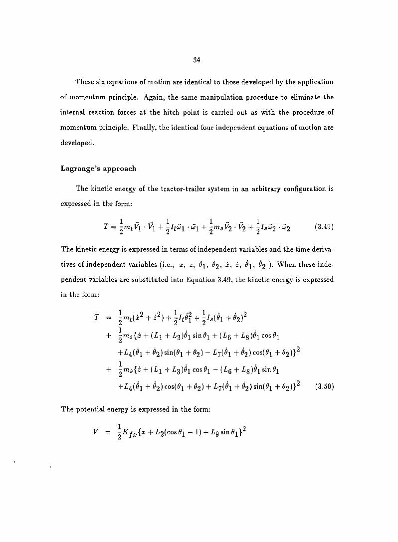
Lagrange's approach

The kinetic energy of the tractor-trailer system in an arbitrary configuration is

expressed in the form:

1 1 _ _ 1 1 ^ ^ T = - m t V i • V i + + 2^5^ • ^2 + 2^51^2 • W2 (3.49)

The kinetic energy is expressed in terms of independent variables and the time deriva­

tives of independent variables (i.e., x, z, 9i, 62, x, z, 62 ). When these inde­

pendent variables are substituted into Equation 3.49, the kinetic energy is expressed

in the form:

^ + z^) + + 2-^-5(^1 + ^2)^

1 + -jms{x + {Li + sin+ (^6 + -^8)^1 cos0]^

-f ^2) sin(^^ -{- ^2 ) " -^7(^1 4" ^2 ) cos(^^ 4- ^2 )}^

1 4- -mg{z 4- (Z/% -H Zg)#! cos 6-^ — (ig 4" 1

+ ^2) cos(^2 +^2)4- &%(#! 4- ^2) sin(0]^ 4- #2)}^ (3.50)

The potential energy is expressed in the form:

^ = ^A'y:j.{x + i2(cos% - l)4-£9sin0l}^

35

+ — L 2 5 m 9 i - { - L ^ { c o s 9 i — ï ) } ^

1 0 + '^Krx{x + Zig sin 9-^ — X]^(cos 9-^ — 1)}

1 0 + 2^rz{- + Z,g(cos — 1) + sin 0]^}

+ + (Xg + Zrg)(cos — 1) + (Ir^ + Zg) sin(^^ + ^2)

+(•^1 + -^3)+ (Xjo — ^7)(cos(^2 + ^2) ~ 1)}^ (3.51)

The formulation of equations of motion based on Lagrange's approach (i.e., Equa­

tion 2.7) does not require a free-body diagram or the introduction and subsequent

elimination of internal forces.

For the first generalized coordinate (i.e., = 2;), the horizontal translational

equation of motion for the tractor-trailer system is expressed in the form:

[ m i -I- mj)z + m s { { L i -f L ^ ) { 9 i sin^^ + cos 9 i )

+(Lg 4- ig)(^\ cos#2 — sin^2) 4- sin(0j 4- ^2)(-^4(^l + ^2)

+-^7(^1 + 6^)2) + cos(^2 + ^2)(-^4(^l + 6^)2 - L ' j { 9 i + #2))}

4-A'yg.{z 4- i2(cos — 1) 4- L Q sin

4-AV.t{® 4- Zg sin 9-^ — Li{cos — 1)} = 0 (3.52)

For the second generalized coordinate (i.e., 92 = z), the vertical translational equation

of motion for the tractor-trailer system is expressed in the form:

{mi 4- m.s)z 4- ms{{Li 4- L^){9i cos 9i - 9^ sin 0j)

- ( L Q 4 - L ^ ) ( 9 I s i n 4 - 9 ^ cos#i) 4- sin(0j^ 4- ^2)(~-^4(^l + 2)^

+^7(^1 + 2)) + cos(^]^ 4- ^2)(-^4(^l + ^2) + ^7(^1 + 2)^)}

4-A'y_{: - 2 sin 4- Ig(cos 9i — 1)}

36

+Krz{z + Xg(cos— 1) + Li sin^]^}

-{•Ks{_z + (Xg + Xg)(cos — 1) + (X^ + Xg) sin

+(X4 + Xg)sin(#]^ + #2) "t" (-^10 ~ Xy)(cos(#]^ + #2) " 1)} — 0 (3.53)

For the third generalized coordinate (i.e., 53 = 6-[), the pitch equation of motion for

the tractor-trailer system is expressed in the form:

IfBi + Isi&i + ^2) + + (X^ + Xg)(^2 cos 9i 4- di sin0]^)

+(Xg -f Xg)(^2 cos 9i — sin#2) + sin(0i + + ^2)

+ L j { è i + 6^)2) -f cos(#2 + #2)(-^4(^1 + 2)^ ~ ^7(^1 + #2))}

{(Xj + L^)SIN9I +(LQ + Xg)cos#i + X^ sin(#2 + ^2)

— Xy cos(#j + 2)} Tng{z + (Xj + X3)(#j cos#} — sin) - (Xg

+Xg)((9]^ sin-f- 9^ cos#^) 4" sin(#2 + 02)(Xy(02 4-1^2) — + 6^)^)

+ cos(#2 + #2)(-^4(^'i + ^2) + -^7(^1 + 2)^)}{(^1 + X3) cos 9 ^

-(Xg + Lg)sin9i -f- X4 cos(#2 + #2) + ^7sin(0j + #2)}

+Kfx{^ + X2(cos — 1) + Xg sin0|}{Xg cos 9^ — X2 sin

+Krx{x + Xg sin#2 — X]^(cos#]^ — l)}{Xg cos#} + X^ sin#2}

—K^^{z — X2 sin+ Xg(cos — 1)}{X2 cos#i 4- Xg sin#2}

+Krz{z 4- Lg(cos9i — 1) -1- sin02}{X]^ cos#} — Xg sin^j}

+Ks{z 4" (Xg 4" Xg)(cos 9i — l)-t-(X]^ 4- X3) sin 9-^ 4- (X4 4- Xg) sin(0]^ + ^2 )

+(-^10 ~ L'j){cos{9i 4- #2) •" 1)}{(-^1 + X3)cos#i — (Xg 4- Xg)sin#i

4-(X4 4- Xg)cos(#2 4- #2) - (-^10 ~ ^7) sin(#]^ 4- #2)} = 0 (3.54)

For the fourth generalized coordinate (i.e., 94 = #2), the relative pitch equation of

37

motion between the tractor and trailer is expressed in the form:

+ ^2) + + {Li + L^){Oi sin4- 0^ cos^j)

+(^g + cos ^2 — sin^]^) + sin(^2 + ^2)

+£7(^1 + 6^)2) + cos(0]^ + 02)(-^4(^I + 2)^ ~ ^ 7 0 1 + ^'2))}

{^4 sin(^2 + $ 2 ) - L ' j cos(^i + ^2)} + "^5(2 + { L i

+Z}g)(^2 cos#i - 2 sin^2) - {LQ + sin^^ + 0^ cosdi)

+ sin(^2 + ^2)(-^7(^'l + ^2) ~ -^4(^1 + ^2)^) + cos(^2 + ^2)(^4(^1 + h )

+ L ' j i è i + 6'2)2)}{l4 cos(0i + O 2 ) + i)7sin(^i + #2)}

+A j{z + (Zg + Zg)(cos — 1) + (Z.]^ + X3) sin

+(^^4 + £5)sin(0]^ +#2) + (Zqo — £7)(cos(^2 + ^2) ~ 1)}

{(X4 4- L^)cos{Oi + #2)- (Liq - Lj)sm(di + ^2)} = 0 (3.55)

For small oscillations about the static equilibrium configuration, Equation 3.52

is the same as Equation 3.32 for horizontal translational motion; Equation 3.53 is the

same as Equation 3.33 for vertical translational motion; Equation 3.54 is the same as

Equation 3.34 for tractor pitch motion; Equation 3.55 is the same as Equation 3.35

for trailer relative pitch motion.

Hamilton's canonical approach

The Hamiltonian function for the vehicle system is expressed in the form:

H = + ^««1 + «2)^

1 + —Tng{z + + L^)0-^ sin+ [ L Q + Xg)^]^ cos 9 - ^

+2,4(^2 + ^2) sin(^2 + ^2 ) — •'^7(^1 ^2) cos(^2 + ^2)}^

38

+ -7?%g{z + + -£3)^1 COS 9-^ — {Lq + Zg)#! sin 6-^

+ L ^ { è i + 2) cos(^i +#2) + L j i è i + $ 2 ) sin(^2 + #2)}^

+ 2^yz{^ + Z'2((:°s^l - 1) + ^9 sin^i}^

+ 2'^yz{^ " 2 sin^i + Zg(cos — 1)}^

1 0 + "^Krxi.^ 4" Z/g sin 9^ — i]^(cos 9-^ — 1)}

+ 2 Arz{z + £g(cos02 — 1) + Z'% sin^]^}^

+ 2 ^a{z + (£5 + •^8)(^°® ^1 - 1) + (i4 + -£5) sin(0]^ + ^2)

+(£1 + £3)sin+ (ZqQ — £%)(cos(^2 + ^2) ~ 1)}^ (3.56)

Hamilton's canonical equations use generalized momenta and generalized coor­

dinates as the state variables which provide a set of 2n first-order equations. For the

first generalized coordinate (i.e., q-^ = x), the horizontal translational momentum of

the tractor is expressed in the form:

Pi = ^ = rrux + ms{x + {Li + L;^)èi sin 61 + { L q + L ^ ) è i c o s 9 i

+ 1,4(^1 + ^2)sin(^i + 2) " + 2) cos(^i + ^2)} (3.57)

For the second generalized coordinate (i.e., ^2 = ~)) the vertical translational mo­

mentum of the tractor is expressed in the form;

P 2 = ^ = r n i z + m s { z + ( L i + L ^ ) 9 i c o s 9 i - { L q + L Q ) 9 i s i n 9 i

+ £4(^1 + 2) cos(gi + ^2) + ^7(^1 + 2) + 2)} (3.58)

For the third generalized coordinate (i.e., 93 = 0^), the pitch momentum of the

tractor is expressed in the form;

d L • . P3 = ^ +-^5(^1 + ^2)

39

+ ms{x + {Li + 1^)01 sin 6i + (^g + L^)0i cos Oi

+ L ^ { é i + 2) sin(^2 + $ 2 ) — L j i & i + ^2) cos(^2 + ^2)}

{(^1 + ^3)sin^i + { L Q + i3)cos^i

+L^ sin(0]^ + 62) - Lj cos(^]^ + 2)}

+ 77%g{z + [L-^ + cos9-^ — (Zg + Zfg)0]^ sin6-^

+-£'4(^]^ + ^2) cos(0]^ 4" ^2) -^7(^1 "I" ^2) sin(0]^ + 2)}

{(£1 + Zg) cos ^2 — (^6 + Z'g)sin^2

+jt^ cos(^2 + ^2) ^7 + 2)} (3.59)

For the fourth generalized coordinate (i.e., = ^2); the pitch momentum of the

trailer relative to the tractor is expressed in the form:

d L P 4 = • ^ = I s { 0 i + e 2 )

+ + { L i + £3)^1 sin^^ + { L q + L g ) 6 i cos^^

-{•L^{9i + 2) sin(^i + ^2) " -^7(^1 + ^2 ) cos(^j + 2)}

{^4 sin(^2 + 6 2 ) — L j cos(^2 + 2)}

+ T n a { z + ( c o s 0 ] ^ — ( Z g + L g ) ^ ^ s i n

+ L ^ { è i + 2) cos(^2 + ^2) + -^7(^1 + ^2) + ^2)}

{^4 cos(^2 + ^2) + 7 sin(0i + ^2)} (3.60)

In order to obtain a set of 2n first-order equations, the generalized velocities are

obtained from the generalized momenta expressions, which are then substituted into

the Hamiltonian function. This involves the inversion of the nxn mass matrix, which

makes it almost impossible to obtain a generalized analytical solution. The common

way to obtain a set of 2n first-order equations of motion for the vehicle system is to

use the generalized coordinates and generalized velocities as the state variables.

The generalized velocities are defined as the state variables:

{i z 6-^ ^2}^ ~ {^1 ^2 ^3 "4}^ (3.61)

The equation of horizontal motion for the vehicle system is expressed in the form:

{ m i + m s ) u i + 5(^0 + Z'g - L Y ) u ^ - r n s L ^ ù ^

+ L ^ { u 2 + «4)'^}

4-(z + ) K { x + L ^ 9 j ^ ) K j ' x =0 (3.62)

The equation of vertical motion for the vehicle system is expressed in the form:

{ m i + m s ) u 2 + r n s { L i + ^3 + 4)^3 + "15^4^14

— ms{LQ + Lg)u'^ + msL'j{u^ + «4)^

— ^2^1) Krz{~ + ^1^1)

+ K s { ~ + { L i + £3)^1 + (^4 + L ^ ) { 6 i + 2)) = 0 (3.63)

The equation of motion for the tractor pitch oscillation is expressed in the form:

ms(Ig + Lg- Lj)ùi + ms{Li + I3 4- L^)il2

+ { I t + I s + f n s { L Q + L g — L j ) ^ + m s { L i + + L ^ ) ^ } u 2

+{Is — msL'^{LQ + Zig — Z^) + msLi^{L-^ + Z3 + £4)104

+ms{LQ + Xg - Ly){{Li + i^3)«3 + £4(1(3 + «4)^)

— m s { L i + £3 + L ^ ) { { L Q + L g ) u ^ — L ' j { u ^ + «4)^)

~^2^fz(~ ~ 2^1) + l^rz(z + £1^1) + LQ KJ J . { X + £9^1)

41

- \ - L ^ K r x { ^ + -^S^l) (^1 + -^3 + -^4 + L ^ ) K s { z + [ L - ^ + -^'3)^1

+(Zi4 + L^){6i + 2)) — 0 (3.64)

The equation of motion for the trailer pitch relative to the tractor is expressed in the

form:

— m s L j i i - ^ + L ^ m s ' i i 2 + {-^s ~ 7?%gZ,y(Z,g + Lg — )

+ -^3 + ^4)}w3 + {-^5 + TRSL J + m s L ^ k / ^

— m s { L ' j { L i + X3) + L / ^ { L Q + L ^ ) ) u ^

+Ks{Li^ + L^)[z + + -^3)^1 + (-^4 + •^5)(^1 + 2)) ~ ® (3.65)

The Equations 3.62 - 3.65 are the first-order equations of motion for tractor-

trailer system in terms of the generalized speeds and generalized coordinates about

static equilibrium configuration. With some simulation programs, the first-order

equations of motion could easily be solved. From the linearized second-order equa­

tions of motion, the mass matrix and stiffness matrix can easily be identified. The

system natural frequencies and vibrational mode shapes are computed from the sys­

tem mass and stiffness matrices. When more complex force input functions are

encountered, the mode superposition technique is applied.

Kane's approach

Kane's method may be used to formulate the equations of motion for this vehicle

model. The generalized speeds are selected to be the first-order time derivatives of

generalized coordinates which are expressed in the form:

{til, U2, U3, «4 = {i, z, ^2}^ (3.66)

42

The velocity at the tractor mass center and the angular velocity of the tractor chassis

are expressed, respectively, in terms of the generalized speeds:

Vi ' +«2^3 (3.67)

0?! = u<^e2 (3.68)

The velocity at the trailer mass center and the angular velocity of the trailer body

are expressed, respectively, in the form:

V 2 = «lê*! + U2e3

+ + L ^ ) s i n6 1 + { L Q + L ^ ) c o s 9 I

+L4 sin(^2 + ^2) ~ -^7 cos(^2 + ^2)1^1

+ [(/;% + Z/g) COS9-^ — {Lq + Zig) sin6-^

+L4 cos(^2 + ^2) + -^7 sin(^]^ + ^2)]^%}

+ sin(^2 + ^2) ~ -^7 cos(^2 + ^2)1^1

+ [£4 cos(^2 + ^2 ) ^7 siu(^2 4" ^2)1^3} (3.69)

'^2 = ^3^2 + "4^2 (3.70)

Spring forces act at the tractor front and rear axles and the trailer axle. The

velocity at tractor front axle centerUne is expressed in terms of the generalized speeds

as:

VJ: = IQEI+-«2E3

+ wglfZg cos — ^2 sin

-[Xg sin0]_ + 2^2 co®^l]^3} (3.71)

43

The velocity at tractor rear axle centerline is expressed in terms of the generalized

speeds as:

V r = + «2^3

+ U3{[Xg cos^j^ + sin0]^]ê*]^

+[—ig sincos (3.(2)

The velocity at the trailer axle centerline is expressed in terms of the generalized

speeds as:

V s = U i ë i + U 2 ë ^

+ L ^ ) s m d i + { L Q + L g ) c o s e i

+(^4 + sin(^2 + ^2) + (^10 " 7) cos(^]^ + ^2)]^1

"^'[(•^1 "f" ^3 ) cos 9-^ — (Zr0 + Xg ) sin

+(14 + Zrg) cos(0j + ^2) ~ (^10 ~ X7) sin(0]^ + ^2)1^3}

+ U4{[(l4 + I5) sin(0]^ + 2) + (^10 — X7) cos(0]^ + ^2)1^1

+ [(•£4 + Z5) cos(^2 + ^2) ~ (^10 ~ Xy) sin(^2 + ^2)!'%} (3.73)

The equations of motion for the system are written in scalar form corresponding

to each generalized speed. Equation 2.15 is expressed in the form:

i = 1, 2, 3, 4 • (3.74)

44

where Fj: , Fr , and Fg are the spring forces as expressed in Equations 3.15, 3.16 and

3.17; F^ and Fg are the inertial forces at the mass center of the tractor and the

trailer, respectively, as expressed in Equations 3.37, 3.38, 3.43, and 3.44; and Tg

are the inertial torque on the tractor and the trailer, respectively, as expressed in

Equations 3.39 and 3.45.

For the first generalized speed (i.e., u-^ = x), the first set of the partial angular

velocity vectors and partial velocity vectors for the tractor and trailer are expressed,

respectively, in the form:

® 1 •

After substituting Equation 3.75 into Equation 3.74 and carrying out the vector dot

product operation, the horizontal translational equation of motion is obtained which

is the same as Equation 3.52.

For the second generalized speed (i.e., wg = z), the second set of the partial

angular velocity vectors and partial velocity vectors for the tractor and trailer are

expressed, respectively, in the form:

After substituting Equation 3.76 into Equation 3.74, the vertical translational equa­

tion of motion for the system is obtained which is the same as Equation 3.53.

For the third generalized speed (i.e., U3 = the third set of the partial

angular velocity vectors and partial velocity vectors for the tractor and the trailer

45

are expressed, respectively, in the form:

dVf — — {Lg cos — ^2 sin

du^

dVy

du^

dVs dw)

^V^

duo

s i du^

duo

1 _

—{LQ sin + L2 cos0j}e3 ;

{ig cos + Lism9i}ei

+{—LQ sin $1 + LI cos O-^JE^ ;

{ ( ^ 1 + + ( Z r g + L ^ ) c o s 6 1

+(^4 + X5)sin(01 +^2)+ (-^10 - 7)008(^1 +^2)}^1

+ { ( ^ % + L^) cos 0-^ — [LQ + Z,g) sin

+(^4 + L^)cos(6 i + 2) ~ (^10 ~ ^7) sin(^i + ^2)1^3 '

0 ;

^ ;

{(III + Zg) sin + (Z-g + Zig) cos $1

+L^ sin(0]^ + $2) — L j cos(^2 + ^2)}^!

4-{(Z2 + Zg) cos ^2 ~ (Zg + Zig) sin

+Z/4 cos(^2 + O2) + Lj sin(^2 + ^2)}^3 '

62 (3.77) ^«3

After substituting Equation 3.77 into Equation 3.74 and carrying out the vector dot

product operation, the rotational equation of motion is obtained which is the same

as Equation 3.54.

For the fourth generalized speed (i.e., U4 = ^2)) the fourth set of the partial

angular velocity vectors and partial velocity vectors of the tractor and trailer are

46

expressed, respectively, in the form:

dVf _ dVr

du^ du/^ = 0 ;

5^4 {(^4 + 5) s in(^ i + Ô2) + {Liq - L' j ) cos{di + 2)}®!

+{(^4 + ^5) cos(l9i + ^2) - (^10 - -ty) sin(i9i + 62)}^^ ;

^ = ^ = 0; du^ ÔU4 '

ÔU4

du^

{^4 sin(^2 + 62) — L j cos(^]^ + ^2)}'^!

+{^4 cos(9 i +62) + Lj sin(^2 + ^2)}^ ;

62 (3.78)

After substituting Equation 3.78 into Equation 3.74 and carrying out the vector dot

product operation, the relative pitch equation of motion for the trailer relative to the

tractor is obtained which is the same as Equation 3.55.

The partial angular velocity vectors and partial velocity vectors are easily ob­

tained once the generalized speeds are defined. The applied active forces and inertial

forces are determined in the same way as in the vector dynamics approaches. Vector

dot product operations require much less effort to obtain the system equations of mo­

tion because there is no introduction of internal forces and subsequent elimination of

them at the geometrical constraints or no complicated mathematical manipulations.

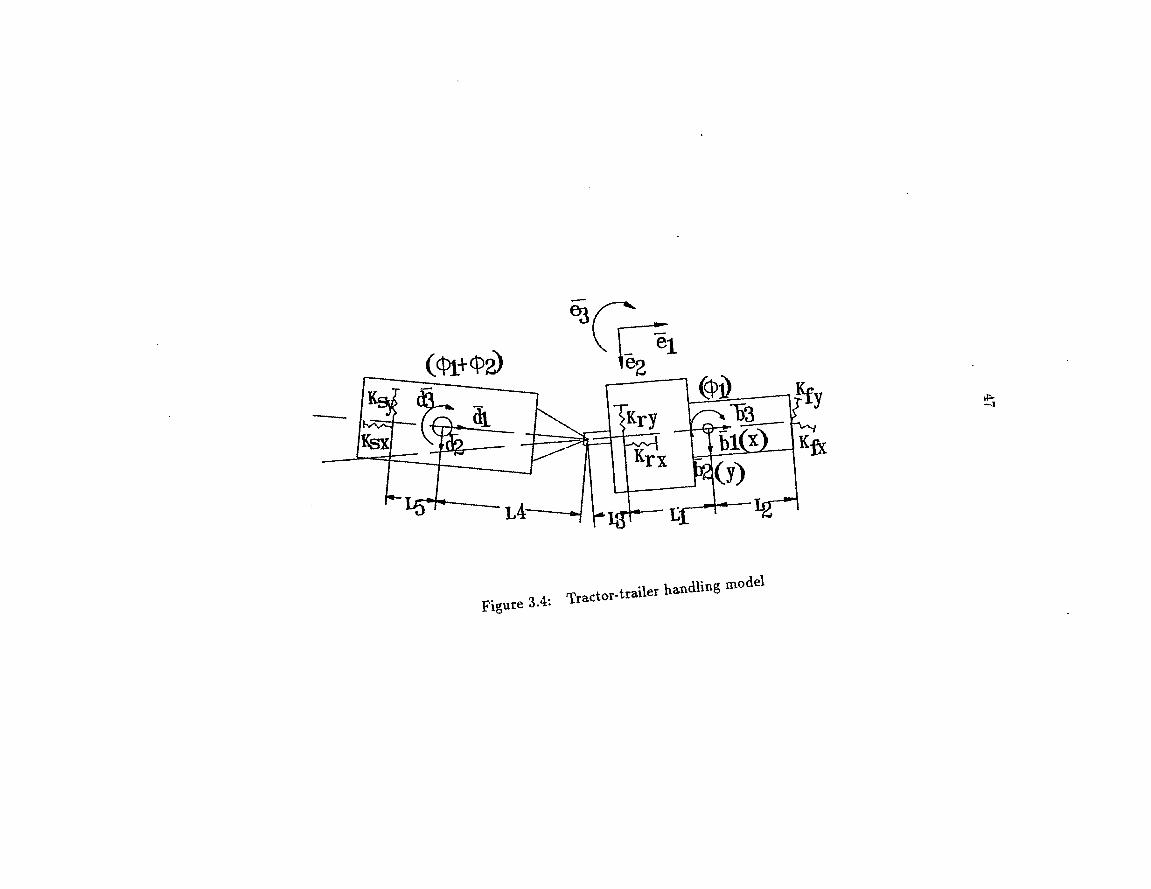
Figure 3.4:

s

trailer handling mod»'

48

Vehicle System Handling Model

The procedure of formulating the system equations of motion is again demon­

strated by a tractor-trailer handling model as shown in Figure 3.4. This simplified

vehicle system model has four DOF: (1) longitudinal translational motion; (2) lateral

translational motion; (3) tractor yaw motion; and (4) trailer relative swing motion

about the hitch point. The resultant tire forces are modelled as linear springs act­

ing at the center of each axle. The orientation of front wheels can be specified and

the spring forces are determined accordingly. Bounce, roll, and pitch motion of the

system are ignored in this handling model.

The inertial frame is defined by the mutually perpendicular unit vectors

and êg; the tractor chassis coordinate system is defined by the unit vectors 6^, 62»

and 63; and the trailer coordinate system is defined by the unit vectors d^, d^, and

jg. At the static equilibrium configuration, three coordinate system axes are parallel

to each other. For planar motion of the vehicle system, the orientation of unit vectors

eg, 63, d^ in the three different coordinate systems remains parallel. The general

relationship between the inertial coordinate system and the tractor chassis coordinate

system at an arbitrary condition is expressed in the form:

n cos 4>l — sin 4)1 0 61

h sin 4>l cos 4>l 0 < h

h . 0 0 1 h.

where 4>i is the rotational angle of the tractor chassis about the 6 3 axis measured in

the inertial frame. The general relationship between the inertial coordinate system

49

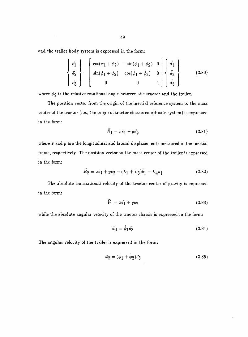
and the trailer body system is expressed in the form;

n

«2

, ^ .

cos(,^]^ + (^62) -sin(^6^ + ^2) 0

sin((?i>i + (/12) cos((^2 + <^2) 0

0 0 1

di

4

(3.80)

where (f>2 is the relative rotational angle between the tractor and the trailer.

The position vector from the origin of the inertial reference system to the mass

center of the tractor (i.e., the origin of tractor chassis coordinate system) is expressed

in the form:

Rl = xei + 2/62 (3.81)

where x and y are the longitudinal and lateral displacements measured in the inertial

frame, respectively. The position vector to the mass center of the trailer is expressed

in the form:

i?2 = xe-^ + 1/62 — (i]^ + L^)b-^ — L^d-^ (3.82)

The absolute translational velocity of the tractor center of gravity is expressed

in the form:

Vi = xei + ye2 (3.83)

while the absolute angular velocity of the tractor chassis is expressed in the form:

wi = 4>ie^

The angular velocity of the trailer is expressed in the form:

^2 = (<^1 + <^2)^3

(3.84)

(3.85)

50

while the translational velocity at the mass center of the trailer is expressed in the

form:

^2 = {i + (^1 + •^'3)<Âl sin

+14(461 + <Â2)sin((^i + ( t>2)}e \

+ {y - {^1 +L^)^ icos4>i

-L4^{4>1 + + 2)}^2 (3.86)

The translational acceleration at the mass center of the tractor is expressed in

the form:

ai^xëi+yë2 (3.87)

while the angular acceleration of the tractor chassis is expressed in the form:

di = <^2 eg (3.88)

The angular acceleration of trailer is expressed in the form:

«2 = (^1 + 2)^3 (3.89)

while the translational acceleration at the mass center of the trailer in the global

coordinate system is expressed in the form:

«2 = ei{x + (Li i-L^)(^is\n(f)i + ^^cos(j)i)

+ L^i ( i j ) i + <^2)W<Al + <62) + (<^1 + <^2)^ cos{( j ) i + (1)2) )}

+ e2{y + (Li + L^){^ ism( j ) i - (j ) icos( f>i )

+ Z'4((<^i + 02)^sin(ç!»i + (?i)2) - (<^1 + <?^2)<^os(<?^l + <^2))} (3.90)

51

At the static equilibrium configuration, (i.e., = (f>2 — 0), the absolute trans-

lational acceleration at the mass center of the trailer can be simplified in the form:

^2 + (-^1 +-^3)^1 + + *^2)^}

+ ^2{i'~ (-^1 + + <^2)} (3.91)

The external spring force applied at the front axle of the tractor is expressed in

the form:

Fj = —{{x + L2{co5( l ) i — l ) ) [Kj:^cos^8 + K^ySivP '8)

+(y + L2sin( f ) i ) {Kj:^ - Kjy)s in8cos8}e i

- {(x + L2{cos (t>i — 1))( A'— K^y) sin 8 cos 8

+(y + I2 sin^2)(Â'yg. sin^ 8 + Kjy cos^ 6)}e2 (3.92)

where Kand Kj y are the resultant spring stiffnesses of tractor front wheels along

the tire plane and perpendicular to the tire plane, respectively; 8 is the front wheel

orientation angle which is a function of the front steering angle and slip angle. The

spring force at the rear axle of the tractor is expressed in the form:

FT = — A7..i;(x + i/]^(l — cos 0]^))ej^

— Kryiy — L\s i i i (j>-^)e2 (3.93)

where Krx and Kry are the resultant stiffnesses of the tractor rear wheels in longi­

tudinal and lateral directions, respectively. The external spring force at trailer axle

is expressed in the form;

Fs = — iiTsxIa: + (^1 + i/3)(l — cos (/»]^) + (^4 + £5)(1 — cos(<^]^ + (^2))}^1

- Ksy{y — {Li + L^)s \n4>i — {L/^ + L^)s in( ( t>i + ( j )2)}e2 (3.94)

52

where Ksx and Ksy are the resultant spring stiffnesses of the trailer wheels in lon­

gitudinal and lateral directions, respectively.

With these defined quantities, the equations of motion for the vehicle system are

constructed through five different procedures in the following subsections.

Momentum approach

Figures 3.5 and 3.6 show the free-body diagram for the tractor and the trailer,

respectively. Px and Py are the longitudinal and lateral internal forces acting on the

trailer hitch point by the tractor, while and Py are the reaction forces acting on

the tractor hitch point by the trailer. The magnitudes of Px and Py equal to the

magnitudes of P^ and Py, but they act in opposite directions, respectively.

The linear momentum of the tractor is expressed in the form:

Lt = rrn{xei + ye2} (3.95)

while the angular momentum of the tractor is expressed in the form:

Ht = (3.96)

where r r i f - is the mass of the tractor; I i is the tractor yaw moment of inertia.

The equations of motion for the tractor are constructed directly by considering

the forces and accelerations in longitudinal and lateral directions, as well as the

rotational torque and angular acceleration about the vertical axis through the mass

center of the tractor. The longitudinal translational equation of motion for the tractor

is expressed in the form:

Ffx + ~ P'x = fnt 'x (3.97)

' %bl(x) ©-

131 Lf

% If 0 cn

CO

Figure 3.5: Free-body diagram of tractor

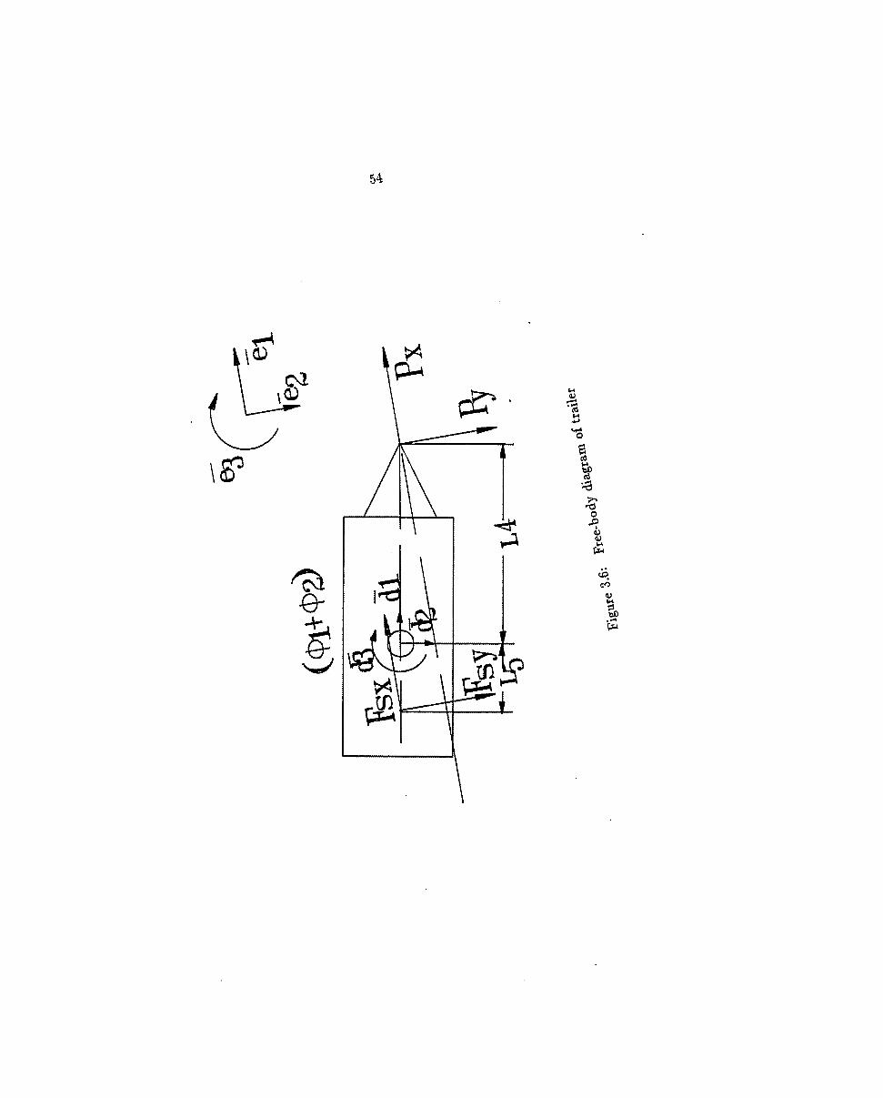
54

&

4 o

Î

I o

%

cc

I

55

The lateral translational equation of motion for the tractor is expressed in the form:

Fjy + Fry - Py = (3.98)

The rotational equation of motion for the tractor is expressed in the form:

— sin(?i>i + L2Fj:y cos <j)i — LiFry cos (l)i + LiFrxsin(j)i

+(Ll + i3)P^cosç!)i - (il + 13)?^ sin 01 = (3.99)

The subscripts x and y are used for the longitudinal and lateral components of the

spring forces at each axle, respectively.

The linear momentum of the trailer is expressed in the form:

Ls = 'msV2 (3.100)

where rris is the mass of the trailer; V2 is the translational velocity at the mass center

of the trailer as shown in Equation 3.86. The angular momentum of the trailer about

its mass center is expressed in the form:

Hs = Isi^i + 2)^^ (3.101)

where Is is the trailer yaw moment of inertia about its mass center.

The longitudinal translational equations of motion for the trailer is expressed in

the form:

Px + Fsx = rns{x + {Li + /^3)(^i sin^;^ + cos (i>i)

+L^{((j)l + (j}2)sm((j)i + (^2) + ("i^l + cos(<^i + (3.102)

The lateral translational equation of motion for the trailer is expressed in the form:

Py + Fsy = msiy + {Li + sin<;6i - cos(?i»]^)

+Li{{^l + (^2)^ + 4)2) - + <i^)cos(,Al + 4>2))} (3.103)

56

where Fsx and Fsy are the longitudinal and lateral components of the trailer wheel

spring forces, respectively. The rotational equation of motion for the trailer about

the mass center is expressed in the form:

— L^Px sin(<^| + <^2) + <^2) sin((^2. + <^2)

-FsyL^ cos((?i»i + ^2) = + ^ 2 ) (3.104)

After the elimination of the inertial forces at the hitch point, (i.e., Pj; = and

Py = Py), four independent equations of motion corresponding to four independent

variables (i.e., x, y, ^2) are obtained. The addition of Equations 3.97 and 3.102

eliminates the longitudinal internal force Px and P^ and produces the longitudinal

translational equation of motion for the vehicle system:

(mi + ms)x + ms{{Li + L^)(^i sin*^^ + cos (pi)

+^4((01 + ^2)si"(<^l + <f>2) + (<Âi + <^2)^cos(<^i + (62))}

= -{(x + L2{COS <1)1 - 1))(A'y-g . cos^ 6 + KJ:Y s in^ S)

+ ( y + L 2 s i n ç i » i ) ( A ' y : . p - K j : y ) s i n 8 c o s 6 }

— K s x { x + (^1 + •^'3)(1 ~ cos<^j) + ( L ^ + L ^ ) { 1 — c o s { 4 > i + 4 > 2 ) ) }

— AVa;{a; + £1(1 - cos(/»j^)} (3.105)

The lateral translational equation of motion for the vehicle system is obtained

by adding Equations 3.98 and 3.103:

(mt +ms)y + ms{{Li + sin^j - (j) i cos( f ) i )

4-^4((<6i + <;^2)^sin(0i + <62) ~ (^1 + <?^,2)cos(+ <?i)2))}

= -{(x + L2{cos( f ) i - l) ){K^y . - K y) s 'm 6 cos 6

57

+(2/ + 2 sinsin^ 6 + K j : y cos^ 6)}

— I^sy{y — {Li + Zg ) sin — (^4 + -^-s) sin(ç!)]^ + (1)2)}

—Kr y {y — s in (3.106)

The rotational equation of motion for the system about the tractor mass center

is obtained by combining Equation 3.99 and Equations 3.102 through 3.104:

{ IT + IS)^I + IS4>2 + + (^1 + ^3)(^1 sin</)i + cos^]^)

+L^{{^1 + <?i2)sin((?i>i + çi>2) + (<Âi + 2)^ cos(çi)i + <^2))}

{{Li + L^)sm4>i + Z,4sin(çii + <^2)}

-ms{y + {Li + L^){4>i sm<f) i - cos4>i)

+L^({^1 + '^2)^sin((^i + <f)2) - + <^))}

{(^l + Ig)coscos(<;6i + (j)2)}

= L2sin( f>i{{x + l2(cos - l))(A''y^ cos^ 6 -f A' sin^ 6)

+{y + ^2 sin0i)(iify:j. - sin 6 cos 6}

— L2 cos(?i)i{(x + L2{cos(f)i - l))(A''y^ - A'y^) sin5cos 5

+(î/ + L 2 S i n ( l ) i ) { K sin^ 6 + K j ^ y cos^ 6)}

—Li sin (^^A'rz(2: + Z]^(l — cosc f )^ ) ) + Li cos 4>iKry{y — sin<^^)

— Rsx{x + (L^ + Zg)(l — cos( j ) i ) + {L^ + L^){1 — cos{( f>i + 1^2))}

{(.^1 + ^3) sin (pi + {L^ + I5) sin(0]^ + (f>2)}

+ I^sy{y — (il + ^3) sin - (£4 + Z5) sin((/>2 + <^2)}

{(Z-i + L;^)cos( f>i + (I4 + L^)COS{(I )2 + ( f>2)} (3.107)

The relative rotational equation of motion of the trailer with respect to the

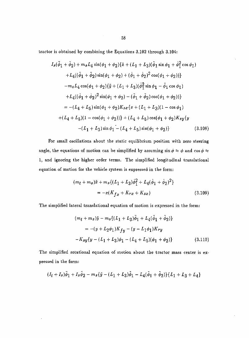
58

tractor is obtained by combining the Equations 3.102 through 3.104:

I s (^ l +^2) + "^-si^4 sin((/>i + + (-^1 +-^3)('?^1 s in( j ) i + ^cos<f) i )

+L^{{^1 + (^2)sin(<?ii +<^2) + (<^1 +<^2)^ cos(<^i + h))}

-msL^cos{( l ) i + ( f )2){y + (^1 + s \n( i>i ~

+L^{{4>1 + (;62)^sin(<6i + <^2) " (^1 + 02)*^os(^l + ^2))}

= "(•£'4 + L^) sin((/)2^ + (j)2)Ksx{x + {L-^ + Z'g)(l — cos 4>i)

+(L^ + Z'g) ( l — cos(ç i ) ]^ + <^2))} + (-^4 + L^)cos(4>I + 4 '2)^sy{y

—{Li + Z,g)sin<^2 — (Z'4 + ^5) sin(i^]^ + <f>2)} (3.108)

For small oscillations about the static equilibrium position with zero steering

angle, the equations of motion can be simplified by assuming sin and cos (j) %

1, and ignoring the higher order terms. The simplified longitudinal translational

equation of motion for the vehicle system is expressed in the form:

{mi + ms)x + ms{{Li + L^)4)^ + L^{^ i + <62)^}

= —x{K + Krx + Ksx) (3.109)

The simplified lateral translational equation of motion is expressed in the form:

{mi + ms)y — Tng{( I ,2 + + -^4(^1 + 2)}

— ~ i y + ~ { y ~ L i 4 > i ) K r y

-Ksy{y — {Li + L^)(f)i — (Z-4 + •^'5)(</'i + 4>2)} (3.110)

The simplified rotational equation of motion about the tractor mass center is ex­

pressed in the form:

{If + Is)^i 4- Is^2 ~ ^s{y - (^1 + ^3)<^i — •^'4(^1 + ^2)}{^1 + -^3 + L^}

59

— I^sy{y — [Li + - {L^ + L^){4>i + çi'2)}{-^i + 13 + ^^4 + L^}

~I '2 iy + fy + l^ry iy — Li<f>i) (3.111)

The simplified rotational equation of motion for the trailer relative to the tractor is

expressed in the form:

+ <f>2) ~ ' f ^sL^ . iy — [L i + L^)4>i — L^{( f ) i + <^2)}

= K s y i L ^ + L^){y — {Li + L ^ ) ( l) i — ( £ 4 + L^)( ( f>i + ^2)} (3.112)

These simplified linear equations of motion for the tractor-trailer system can be

rearranged in the matrix form:

[M]{q} + [K]{q} = {F} (3.113)

where vector {q} '^ is the independent variable which is defined as {z, y , ( f>i , <^2}^:

{F} i s the force vec tor which conta ins the equiva lent sys tem exci ta t ion forces ; [M]

and [K\ are the 4x4 system mass and stiffness matrices, respectively. The elements

of the matrices and th? force vector are listed in Appendix B.

D'Alembert's approach

D'Alembert's principle can be used to formulate the system equations of motion

by considering the dynamic equilibrium of the active and inertial forces for each body.

The translational inertial force for the tractor is expressed in the form:

= -nnxei - (3.114)

while the inertial torque for the tractor is expressed in the form:

^1 = -hHh (3.115)

60

The longitudinal translational equation of motion for the tractor is obtained by

summing the active and inertial forces in the direction:

Ff^ + Frx-Px + ^lx-^ (3,116)

while the lateral translational equation of motion for the tractor is obtained by sum­

ming the active and inertial forces in the direction:

^fy ~ ^ly ~ ® (3.117)

The equilibrium of the active and inertial torques about êg axis through the mass

center of the tractor generates the tractor rotational equation of motion;

-1-2 F J J , s in <f>i + L2 Fjy cos 4>i + LiFrx — -^1 Fry cos 4>i

•\-{Ly "H )Py (-OS(^2 — (^1 Z/g)f;p sin ( f ) -^ + = 0 (3.118)

where F^^ and F^y are the inertial force components in and 6*2 directions, respec­

tively.

The inertial forces for the trailer is expressed in the form:

^2 = -ms{x + {Li + L^) (^ i s in ( f ) i + cos ( f ) i )

+^4((<^1 + + <^2) + (^1 + <62)^ cos((?!)i + ( l )2) )}ê i

- ms{y + (Li + L^){^i sin<61 - cos) 4- £4((<Âl

-t-<^2)^sin((/iii 4- (j)2) - (<^1 + ^2)cos((?i»i -H <^2))}^ (3.119)

while the inertial torque about the trailer mass center is expressed in the form:

T2 = —•^^(«^i + 2)^3 (3.120)

61

The equilibrium of the active and inertial forces in the longitudinal and lat­

eral directions produces the translational equations of motion for the trailer in the

longitudinal and lateral directions, respectively:

Px + P'sx "f F2X ~ ® (3.121)

Py + Fsy + i^2y ~ 0 (3.122)

The equilibrium of the active and inertial torques about the mass center of the trailer

produces the trailer rotational equation of motion:

-L^Px + 2) + ^4% cos(çi)]^ + 2)

+FsxL^ sin((^2 + ^2) ~ cos((^]^ + 1^2) + ^2 ~ ^ (3.123)

After the substitution of tractor inertial forces into Equations 3.116 to 3.118,

three equations of motion for the tractor are obtained which are the same as Equa­

tions 3.97 to 3.99. The substitution of trailer inertial forces into Equations 3.121

to 3.123 produces the equations of motion for the trailer, which are the same as

Equations 3.102 to 3.104. Again, the same manipulation procedure to eliminate the

internal forces at the hitch point is carried out as with the procedure of the momentum

principle approach. Four identical system equations of motion are then obtained.

Lagrange's approach

Lagrange's method can be used to formulate the system equations of motion

directly from the energy functions of the system. The kinetic energy of the vehicle

system is expressed in the form:

^ + 2'^5(<6i + <^2)^

62

+ ^ms{x+ {Li +L^)^ i s in <f>i

+-£4(^1 + <^2)sin(<?i'i + 4>2)} '^

1 + 2^s{y - {Li + L:^)<f>icos( j ) i

— + <^2) ^2)}^ (3.124)

The potential energy of the system due to the linear spring deflections is expressed

in the form:

V = - A'yr^{(a; + Ir2(cos — 1)) cos 5 + (2/+ ^2 sin sin (5}^

+ ^Kj :y{{x + JD2(cos<;!n - 1)) sin6 - (y + X2 sin <;/>! ) cos 6}^

+ 2^^rx{x + •£'i( 1 — cos)}^ + 2Ar!/{!/ ~ -^1 sin4>\}^

+ •^ f^sx{x + {Li + Z,g)(l - cos 4- + fg)(l - cos{( f>i + <f>2))}^

+ - (-^1 + •t'slsinçi)]^ — (Z-4 + i5)sin((?i)]^ + <^2)}^ (3.125)

There are no other external applied forces. The equations of motion correspond­

ing to each independent variable can be formulated by performing the derivative

operations:

where is the independent system variable (i.e., {a:, y , ( j )^ , 4>2} '^ ) -

For the first generalized coordinate (i.e., q-^ = x) , the longitudinal translational

equation of motion for the vehicle system is expressed in the form:

{mi + ms)x + + L-^){<j>i sin^j + cos</)i)

+^4(('^1 + + (f>2) + + <62)^ cos{4) i + <f)2) )}

+ K^j, { {x + £2(005 ( j ) i — 1)) cos 6 + {y + L2 sin (j^j) sin5} cos 6

63

+A'f y{{x + L2{cos ( f ) i — 1)) sin 5 — (1/ + L2 sin 4>i)cos 6} sin 6

-\-Krx{,^ + -^1(1 ~ cos(^2)} + Ksx{'^ + (-^1 + )( 1 — cos^j^)

+(•£'4 + L^){1 — cos((^2 + <^2))} ~ 0 (3.127)

For the second generalized coordinate (i.e., gg = y)i the lateral translational

equation of motion for the vehicle system is expressed in the form:

{mi + ms)y + ms{iLi + sinçi>i - cos)

+L^{{^1 + (^2)^s in(<Al + <l>2) - (^1 + 2)cos(<^i + «Ag))}

+KJ^{(x + 12(005 (i>i — 1)) cos 5 + (y + 2^2 sin 0]^) sin^} sin 6

— Kfy{{x + £2(005 <^i — 1)) sin S - (7/ + ^2 sin </)]^) cos 5} cos S

+ Asy{î/ - (£i + fg) sin<pi - (X4 + ig) sin((?iij + (^2)}

+Â7't/{y — sin(^2^} = 0 (3.128)

For the third generalized coordinate (i.e., gg = (^j), the rotational equation of

motion of the vehicle system about the mass center of the tractor is expressed in the

form:

(/( + £3)^1 + fs^2 + + (£1 + £3)(^i sinc^i + 00s <^i)

+£4((^1 + <^2)sin(<Al + <^2) + (<^1 + <^2)^ cos((^i + <^2))}

{(^1 + £3)5111^1 + l4sin(<^i 4- <62)}

-ma{y + (^i + i^3)(<^f sinc^i - 005 (/>i)

+£4(((^1 + <Â2)^sin(<^i + <^2) - (<^1 + ^2)^°^('^1 + <^))}

{(Il + £2)005(^1 + cos((6i + <^2)}

+Kyg.{(z + L2(cos ( f>i — 1)) cos 8 + (y + £2 sin (^1) sin 5}

64

{ — ^2 cos 5 + ^2 cos <i>i sin 5}

—K+ 2(005 ( f>-^ — 1)) sin6 — (y + Z2 sin 4>i) cos 6}

{L2 sin (j>i sin 5 + £2 cos (f>i cos 6}

+Krx{^ + -^1(1 - cos ( f ) i ) }L i sin— Kry{y - sin^^}^^ cos ( j ) i

+Ksx{x + (^1 + • i '3 ) ( l — cos ( j ) i ) + (Z4 + Z,g) ( l — cos( (^2 + ( l>2))}

{(I r i + Zrg) s in(^2 + (£ .4 + L^)sm{( f ) i + 4>2)}

— Ksy{y — {L i + Z3)sin0]^ — (Z4 + £5)sin(<^2 + (f>2)}

{(Li + L^)cos(f>i + (£4 + L^)cos{(t)i + (^2)} = 0 (3.129)

For the fourth generalized coordinate (i.e., 54 = <p2), the relative rotational

equation of motion for the trailer is expressed in the form:

h{(i>l + <^2) + + (£1 + sin<;6i + <6^ cos

+L^{((I>1 + <A2)sin((Ai + <P2) + (<^1 + <^2)^cos(<;62 + (?i>2))}{£4 sin(çi>i + <^2)}

-ms{y + {Li + L;^){^^s in( f ) i - coscpi )

+-£4((<i>l + <;62)^sin((^i + <62) - (<Al + <i^2)cos(<^i + çi>2))}{£4 cos(<?i)i + <^2)}

+^sx{^ + (^1 + •^'3)(1 — cos <^2 ) + (Z4 + £g)(l

- cos(çi.i + 4>2))}{{L^ + £5) sin{<f)i + .^2)}

— I^sy{y — {Li + £3) sin ( f>i — (X4 + Z5) sin((/)]^ + <^2)}

{ (X4 + l5)cos(0i + 02)} (3.130)

Equations 3.127 - 3.130, which are the same as Equations 3.105 - 3.108 obtained

through the momentum principle approach, are obtained directly from the derivative

operations on the system energy functions. The Lagrangian approach to formulate the

65

system equations of motion does not require a free-body diagram or the introduction

and subsequent elimination of internal forces.

Hamilton's canonical approach

Hamilton's canonical approach to formulate the system equations of motion re­

sembles the Lagrange's equation approach, except the Hamiltonian function is the

total energy of the system. The system equations of motion are expressed in a set

of 2n first-order differential equations with generalized coordinates and generalized

momenta as the state variables. This method provides the momentum function of

the system, but the final equations of motion are difficult to obtain and are not used

as widely as the Lagrange's equation approach.

The Hamiltonian function of the system for the vehicle system is expressed in

the form:

1 + - m s { x + { L i + s i n ( l > i

-t- <?2) sin((?i)]^ + <62)}^

1 + 2^s{y - (Li + L^)4>lcos( l ) i

-L^(4>1 + <Â2)cos(<^i + 4)2)}^

1 '2 + -K-f L2{cos(f>i — 1)) cos 6 + (y + 2^2 sin (^i)sin6}

2 *2 + -Kj :y{(x + X2(cos<?i>i - l))sin(5 — {y -f X2 sin cos 5}

+ 2^^rx{x + ^1(1 — cos + 2 sin (^2}^

+ -Ksx{x + (Z-i + — cos4>i) + {L^ + - cos(<^2 + 1^2))}^

66

+ — (^1 + ^3) sin <62 — + Z_^) siii(^2 + <^2)}^ (3.131)

The generalized momentum corresponding to each independent variable is com­

puted from the Hamiltonian function. For the first generalized coordinate (i.e.,

qi = a;), the longitudinal translational momentum of the system is expressed in

the form:

dH Pi = — rrux + Tns{x + {Li + L^)^ is 'm( l ) i

+ 'P2)} (3.132)

For the second generalized coordinate (i.e., q2 = y) , the lateral translational mo­

mentum of the system is expressed in the form:

dH P.2 = — = mfy 4- - (1% 4- cos (pi

- + 4>2)cos{(pi+(f>2)} (3.133)

For the third generalized coordinate (i.e., gg = 0]^), the yaw momentum of the

system about the tractor mass center is expressed in the form:

dH • . Pz = = IfPl + + <^>2)

0(pi

+ ms{x + (L i + 13)^1 sin(?i>i + -H <^2) sin(<?!»i + <^)}

{(Il + L^)sm<f) i + I4 sm{( t ) i + <^2)}

- rns{y - {Li + L'^)4>1 cos(pi - -f 4>2)cos{4>i + (^2)}

{(^l + ^3) cos (j)i -f- I4 cos(0^ 4- 02)} (3.134)

Finally, for the fourth generalized coordinate (i.e., — 02)) the swing momentum

of the trailer with respect to the tractor is expressed in the form:

dH • • ^4 = 7j-= ^(01 + 02)

C02

67

+ ms{x + {Li + L^)^ i s in<1)1 + L^{<j) i

+4>2)sm{(i)i +9l'2)}{-^4 siii(<Al +02)}

- rns{y - {Li + L2)4> I cos 4>i - L^i^ i

+^2) + ^^2)}{^4 cos(<^i + <62)} (3.135)

The relationship between generalized momenta and generalized speeds must be

solved from the definition equations. The Hamiltonian function is then represented in

terms of generalized momenta and generalized coordinates. This approach to get a set

of first-order differential equations requires many more mathematical operations than

the commonly used methods in which the generalized coordinates and generalized

speeds are used as the state variables.

The first-order equations of motion about the static equilibrium position with

rotation angle of zero for the front wheels are obtained by defining the generalized

speeds as the state variables:

The other four first-order equations are obtained from the simplified second order

equations generated by using momentum principle approach.

The longitudinal translational equation of motion for the system about the static

equilibrium position is expressed in the form:

The lateral translational equation of motion for the system about the static equilib­

(3.136)

{rrn + ms)ûi + ms{(Li + L^)u^ + 14(^3 -f «4)'^}

(3.137)

68

rium position is expressed in the form:

{mt + ms)u2 - ms{{Li + 13)113 + L^iù^ + «4)}

= -{y + L2( f>i)K^ y - {y - Li( f ) i )Kry

—Ksy{y — (-^1 + L<^)(j)-i — (£4 + + ^2)} (3.138)

The equation of motion for the tractor yaw oscillations about the tractor mass center

is expressed in the form:

ih + s )^Z + 'S"4 — ' rns{Û2 — (^1 + ^3 )^3

--^4 ("3 + + -^3 + ^4}

= I i sy{y — (L i + L^)4>i — (Zr4 + L^){( f ) i + 4>2)}{^1 + 3 + L^ + X5}

~^2^y fy "t" Lihry iy — -t'l'^i) (3.139)

The equation of motion for the trailer swinging relative to the tractor is expressed in

the form:

• ^ s ( " 3 + " 4 ) — msL^{Ù2 — {L-^ + 3 ) ^ 3 — ^ , 4 ( ^ 3 + Û 4 ) }

= A5y(I<4 + L^){y - (Li + L^)<f) i - (L4 + L^){<i>i + <j)2)} (3.140)

Together with the definition of generalized speeds (i.e., Equation 3.136), eight

first-order differential equations are obtained.

Kane's approach

Kane's method begins with the definition of the generalized speeds. To get the

system equations in the same form as those obtained from the previous methods, the

69

first-order time derivatives of the generalized coordinates are defined as the general­

ized speeds.

{«1, U2, «3, «4}^ = {x, t/, <^1, ^2}^ (3.141)

The translational velocity at the mass center of the tractor, and the angular

velocity of the tractor chassis are expressed, respectively, in terms of the generalized

speeds as:

Vi = u-^ei + «262 (3.142)

= "3^3 (3.143)

The velocity at the mass center of the trailer, and the angular velocity of the trailer

body are expressed, respectively, in terms of the generalized speeds as:

V2 = -h 13)^3 sin01-1-14(^3-1-«4) sin(ç!>i + çi>2)}

+ e2{u2-{Li +L^)u^cos(l)i-L^{u^ + u^)cos{<f)i + (f>2)} (3.144)

^2 = ("3 + ^4)^3 (3.145)

There are spring forces acting at the tractor front and rear axles, and the trailer

axle. The velocity at the centerline of each axle where the active force is applied

needs to be determined so that the contribution of each active force to the system

equations can be evaluated through vector dot product operation.

The velocity at the tractor front axle center point is linearly expressed in terms

of the generalized speeds as:

Vf = - l2^3s i i i<6i}

+ e2{u2 + L2U2 cos ( j ) i } (3.146)

70

The velocity at the tractor rear axle center point is linearly expressed in terms of the

generalized speeds as:

Vr = + ^1^3 sin <^2}

+ — -^1^3 cosf;^^} (3.147)

The velocity at the trailer axle center point is linearly expressed in terms of the

generalized speeds as:

Vs = + 13)^3 sin (/»!

+(£4 + L^){u^ + u^)s in{( j ) i + ^2)}

+ e2{w2 - (i^i + X3)u3cos0i

— (Zf4 + + W4) cos(<^]^ + 4'2)} (3.148)

The active forces applied to the system are the spring forces as shown in Equa­

tions 3.92 - 3.94. The inertial forces and torques for the tractor and trailer are defined

as in D'Alembert's principle approach. The system equations of motion correspond­

ing to each of the four generalized speeds are obtained by performing the vector dot

product operation:

i = 1, 2, 3, 4 (3.149)

For the first generalized speed (i.e., u-^ = x), the first set of the partial angular

velocity vectors and partial velocity vectors for the tractor and trailer are expressed,

71

respectively, in the form:

After substituting these quantities into Equation 3.149 and carrying out the vec­

tor dot product operation, the longitudinal translational equation of motion for the

system is obtained, which is the same as Equation 3.105.

For the second generalized speed (i.e., «2 = y), the second set of the partial

angular velocity vectors and partial velocity vectors for the tractor and trailer are

expressed, respectively, in the form:

9% = "2; §%=»:

After substituting these quantities into Equation 3.149 and carrying out the vector

dot product operation, the lateral translational equation of motion for the system is

obtained, which is the same as Equation 3.106.

For the third generalized speed (i.e., wg = ), the third set of the partial angular

velocity vectors and partial velocity vectors for the tractor and trailer are expressed,

respectively, in the form:

5 "

72

dûj i

duz

Ê È 9U3

du^

dVf

dVr

du 2,

dVs

ÔU3

^3;

ë i{[Li + i;3)sin(?ii + L4^sm{( f>i + <^2)}

-ê*2{(^l + ^3) cos (Al + ^4 cos((^i + (1)2)} ' ,

G3;

— L2 sin (pl^l + ^2 cos (f>ie2',

Li sin<f>iei — cos

e i{{Li + Lz)sm( t>i + (£4 + L^)sm(( t>i + <^2)}

-ê2{(-^l + l3)cos<Ai + (I4 + L^)cos{(f>i + <^2)} (3.152)

After substituting these quantities into Equation 3.149 and carrying out the vector

dot product operation, the rotational equation of motion for the system about the

tractor mass center is obtained, which is the same as Equation 3.107.

For the fourth generalized speed (i.e., «4 = ^2), the fourth set of the partial

angular velocity vectors and partial velocity vectors for the tractor and trailer are

expressed, respectively, in the form:

dVi 0;

0;

^ = e i{L^sm(( j ) i+( l )2)}

du^

dCJi du^

h '4

gw 2 duA

-e2{L^cos(4>i + 4>2)};

G3;

73

5^4 5U4 ' ay, — = ë i { { L ^ + L ^ ) s m { ( l ) i + 4 > 2 ) }

-é2{(^4 + 5)cos(0i + 02)} (3.153)

After substituting these quantities into Equation 3.149 and carrying out the vector

dot product operation, the rotational equation of motion for the trailer relative to

the tractor is obtained, which is the same as Equation 3.108.

74

CHAPTER 4. GENERAL-PURPOSE COMPUTER SIMULATION

PROGRAMS

Multibody geometrically-constrained mechanical systems simulation programs

have been developed to predict the dynamic response of mechanisms and to optimize

their performance. The main advantages of this multibody simulation software are:

(1) automatically generate the equations of motion and solve them numerically; (2)

solve the kinetostatic problem; and (3) provide 'user-friendly' pre and post-processor

capabilities.

Typically, a problem-oriented language is used to define the system configuration

in terms of (1) joints by type, (2) bodies with inertial properties, (3) geometry,

(4) translational and rotational springs and dampers, (5) linear and nonlinear force

and motion inputs, and (6) special 'user-defined' capabilities. Also, these programs

have the following design capabilities: (1) static equilibrium position analysis, (2)

large displacement (nonlinear) transient analysis, (3) linearized oscillation vibrational

analysis, and (4) graphical display.

This group of simulation software uses five methods to formulate the system

equations of motion. Table 4.1 summarizes most of the currently available software

packages. This table contains for each program most of the applicable references;

the particular method to formulate the system dynamical equations, characteristics

75

related to coordinate selection and special numerical algorithms, special remarks and

applications.

Table 4.1: Multibody simulation software packages

Program Formulation Methodology and Remarks Applications Name Characteristics

ADAMS and Lagrange's method with La- Spatial and planar analysis; Kine- Machinery; Vehicle DRAM grangian multipliers; Cartesian matic static and dynamic force systems; Robots [79-104] coordinates; Sparse matrix formu- analysis; Open and closed loops;

lation; ODE and algebraic solu- Rigid and flexible bodies; Inter-tion active user interface; Kinematic

joint library

Lagrange's method with La- Spatial and planar analysis; Static Machinery; Vehicle grangian multipliers; ODE nu- and dynamic force analysis; Open systems; merical integration; QR decom- and closed loops; Rigid bodies; position; Lagrangian coordinates; Control elements; Kinematic joint Sparse matrix formulation library

DADS Lagrange's method with La- Spatial and planar analysis; Kine- Machinery; Robots; [107-133] grangian multipliers; DE numer- matic, static and dynamic force Vehicle systems

ical integration ; Cartesian and analysis; Open and closed loops; modal coordinates Rigid and flexible bodies; Control

elements; Interactive user inter­face; Kinematic joint library

Lagrange's method with La Spatial and planar analysis; Static Machinery; Vehicle grangian multipliers; DE numer- and dynamic force analysis; Open systems ical integration; Cartesian and and closed loops; Rigid and flexi-modal coordinates ble bodies

CAMS [105-106]

DAMS [134-150]

Table 4.1 (Continued)

Program Name

Formulation Methodology and Characteristics

Remarks Applications

DYMAC [151-157]

Lagrange's form of d'Alembert's principle; Lagrangian coordinates

Spatial and planar analysis; Kine­matic, static and dynamic force analysis; Open and closed loops; Rigid bodies

Machinery; Robots

IMP Lagrange's method; Lagrangian Spatial and planar analysis; Kine- Machinery; Robots; [158-170] coordinates; Eigenvalue numerical matic, static and dynamic force Vehicle systems

integration; Optimum generalized analysis; Open and closed loops; coordinate selection Rigid bodies; Flexible bodies (in

preparation); Kinematic joint li­brary; Interactive user interface

MCADA [171-172]

Lagrange's method with La­grangian multipliers; Gear's inte­gration method; Cartesian coordi­nates

Planar systems; Kinematic, static and dynamic force analysis; Open and closed loops; Rigid bodies

Machinery; systems

Vehicle

SD/EXACT [173-174]

Kane's method; Symbolic formu­lation; Relative coordinates

Spatial and planar systems; Dy­namic force analysis; Rigid bodies; Tree structures; Cîontrol elements

Vehicle Robots

systems;

TREETOPS [175-179]

Kane's method; Relative coordi­nates

Spatial and planar systems; Dy­namic force analysis; Rigid and flexible bodies; Tree structures; Control elements

Vehicle Robots

systems;

Table 4.1 (Continued)

Program Formulation Methodology and Remarks Applications Name Characteristics

VECNET Newton-Euler method; Cartesian Spatial and planar systems; Static Machinery [180-185] coordinates and dynamic force analysis; Rigid

bodies NUSTAR Articulated-body inertia method; [55, 62] Lagrangian coordinates; La-

grangian multipliers

Spatial and planar systems; Static and dynamic force analysis; Rigid and flexible bodies; Open and closed loop; Interactive user inter­face; Kinematic joint and compo­nent libraries

Machinery; Vehicle systems

S

MEDYNA Newton Euler method; La-[186] grangian coordinates; Small dis­

placement formulation

Spatial and planar systems; Dy­namic force analysis; Rigid and flexible bodies; Interactive user in­terface

Vehicle systems

NEWEUL Newton-Euler method; Cartesian [187] and Lagrangian coordinates; Sym­

bolic/numeric equations

Spatial and planar systems; Open and closed loops; Kinematic con­straint library; Rigid bodies

Machinery; Vehicle systems

79

CHAPTER 5. SUMMARY

Five different principles which provide the theoretical bases for developing gen­

eral purpose, multi-body simulation programs are reviewed. The procedure of using

each of the five methods to formulate system equations of motion is demonstrated

through simplified tractor-trailer ride vibration and handling models.

Vector dynamics (i.e., the Momentum principle and the D'Alembert's principle)

are used to formulate system equations of motion by relating the motion and the

force on each body separately. The physical meanings are well preserved, but the

introduction and subsequent elimination of internal forces make it difficult to achieve

the final system equations of motion.

The energy approach (i.e., the Lagrange's method and the Hamilton's canonical

method) makes use of the system kinetic and potential energy functions, which are

scalar values and can be linearly added together. The system equations of motion

corresponding to the independent variables are formulated through partial derivative

and total derivative operations. This is a systematic approach, but less physical

meaning is preserved.

Kane's method provides the opportunity for convenient generalized speed defi­

nitions. The velocity and angular velocity functions can be linearly represented in

terms of those generalized speeds. The partial velocity of a point and partial angular

80

velocity of a body can be identified by inspection. The system equations of motion

are constructed by vector dot-product operations which are much simpler than the

derivative operations. This method requires the least effort in formulating equations

of motion by hand.

Existing multi-body, geometrically-constrained mechanical systems simulation

software has been summarized according to the particular principle used to formulate

the system dynamical equations, special analysis capabilities, and applications.

81

BIBLIOGRAPHY

Analytical Dynamics for Multi-body Systems

[1] Kane, T. R., and D. A. Levinson. 1980. Formulation of equations of motion for complex spacecraft. J. Quid. Control 3(2):99-112.

[2] Paul, B. 1984. Computer-oriented analytical dynamics of machinery. Computer-Aided Analysis and Optimization of Mechanical Systems Dynamics, Series F: Computers and System Science 9:49-88. Springer-Verlag, New York.

[3] Paul, B. 197.5. Analytical dynamics of mechanisms - A computer oriented overview. Mechanism and Machine Theory 10:481-507.

[4] Paul, B. 1979. Kinematics and dynamics of planar machinery. Prentice-Hall, Englewood Cliffs, NJ.

[5] Sandor, G., and A. Erdman. 1984. Advanced Mechanism Design: Analysis and Synthesis. Volume II. Prentice-Hall, Englewood Cliffs, NJ.

[6] Wells, D. A. 1967. Lagrangian dynamics. McGraw-Hill Book Co., New York.

[7] D'Souza, A. F., and V. K. Garg. 1984. Advanced dynamics: Modeling and analysis. Prentice-Hall, Englewood, Cliffs, NJ.

[8] Collar, A. R., and A. Simpson. 1987. Matrices and engineering dynamics. Ellis Horwood Ltd., London.

[9] Haug, E. J. 1989. Computer-aided kinematics and dynamics of mechanical sys­tems. Vol. I - Basic methods. Allyn and Bacon, Boston.

[10] Haug, E. J. 1990. Intermediate dynamics. Allyn and Bacon, Boston.

[11] Wittenburg, J. 1977. Dynamics of systems of rigid bodies. Teubner, Stuttgart.

82

12] Truesdell, C. 1968. Essays in the history of mechanics. Springer Verlag, New York.

13] Nikravesh, P. E. 1988. Computer-aided analysis of mechanical systems. Prentice-Hall, Englewood Cliffs, NJ.

14] Shabana, A. 1989. Dynamics of multibody systems. Wiley and Sons, New York.

15] Rouse, N. E. 1988. Dynamic analysis takes on a new look. Machine Design 60(5):98-101.

16] Rouse, N. E. 1987. Modeling dynamic mechanical systems. Machine Design 59(19):76-80.

17] Rouse, N. E. 1986. Mechanical simulation comes of age. Machine Design 58(4):60-65.

18] Mills, R. B. 1986. Software simulates mechanical systems. Computer-Aided Engineering 5(3):36-44.

19] McConville, J. B. 1985. Safer designs through dynamic simulations. Computer-Aided Engineering 4(1)-.36-40.

Kane's Method (Lagrange's form of d'Alembert's principle)

20] Kane, T. R., and D. A. Levinson. 1985. Dynamics: theory and applications. McGraw-Hill Book Co., New York.

21] Kane, T. R., P. W. Likins, and D. A. Levinson. 1983. Spacecraft dynamics. McGraw-Hill Book Co., New York.

22] Kane, T. R., and D. A. Levinson. 1983. Multibody dynamics. ASME J. Appl. Mech. 50:1071-1078.

23] Kane, T. R., and S. Djerassi. 1987. Integrals of linearized differential equations of motion of mechanical systems. Part I: Linearized differential equations and Part II: Linearized equations of motion. ASME J. Appl. Mech. 54:656-667.

24] Kane, T. R. 1961. Dynamics of nonholonomic systems. ASME J. Appl. Mech. 28:574-577.

25] Kane, T. R. 1973. Solution of kinematical differential equations for a rigid body. ASME J. Appl. Mech. 40:109-113.

83

[26] Kane, T. R., and D. A. Levinson. 1983. The use of Kane's dynamical equations in robotics. Int. J. Robot. Res. 2(3):3-21.

[27] Faessler, H. 1986. Computer-assisted generation of dynamical equations for multibody systems. Int. J. Robot. Res. 5(3):129-141.

[28] Kane, T. R., R. R. Ryan, and A. K. Banerjee. 1987. Dynamics of a cantilever beam attached to a moving base. J. Quid. Control Dyn. 10:139-151.

[29] Ryan, R. R., and T. R. Kane. 1985. Dynamics of a modular space station. J. Astronautical Sci. 33(4):381-400.

[30] Ryan, R. R. 1986. Flexibility modeling methods in multibody dynamics. Ph.D. dissertation. Stanford University (Libr. Congr. Microfilms 8612787). Univ. Mi­crofilms Int., Ann Arbor, Michigan.

[31] Djerassi, S., and T. R. Kane. 1985. Equations of motion governing the deploy­ment of a flexible linkage from a spacecraft. J. Astronautical Sci. 33(4):417-428.

[32] Levinson, D. A., and T. R. Kane. 1983. Docking of a spacecraft with an unre­strained orbiting structure. J. Astronautical Sci. 31(l):23-48.

[33] Levinson, D. A., and T. R. Kane. 1981. Simulation of large motions of nonuni­form beams in orbit: Part I - The cantilever beam. J. Astronautical Sci. 29(3):213-244).

[34] Kane, T. R., and D. A. Levinson. 1981. Simulation of large motions of nonuni­form beams in orbit: Part II - The unrestrained beam. J. Astronautical Sci. 29(3):245-275).

[35] Huston, R. L., and C. E. Passerello. 1980. Multibody structural dynamics in­cluding translation between the bodies. Comp. and Struct. 12:713-720.

[36] Huston, R. L. 1981. Multibody dynamics including the effects of flexibility and compliance. Comp. and Struct. 14:443-451.

[37] Huston, R. L. 1985. Useful procedures in multibody dynamics, p. 69-77. in G. Bianchi and W. Schiehlen (ed.) Dynamics of multibody systems. lU-TAM/IFToMM Symposium Udine/Italy. Springer-Verlag, New York.

[38] Huston, R. L. 1986. Computing angular velocity in multibody systems. Eng. Comput. 3:223-229.

84

Buffinton, K. W. 1985. Dynamics of beams moving over supports. Ph.D. Disser­tation. Stanford University (Libr. Congr. Microfilms 8602460). Univ. Microfilms Int., Ann Arbor, Michigan.

Amirouche, M. L. 1986. Dynamic analysis of 'tree-like' structures undergoing large motions - a finite segment approach. Engineering Analysis 3(2):111-117.

Nielan, P. E. 1987. Efficient computer simulation of motions of multi-body systems. Ph.D. Dissertation. Stanford University (Libr. Congr. Micro­films 8707714). Univ. Microfilms Int., Ann Arbor, Michigan.

Desloge, E. A. 1987. Relationship between Kane's equations and the Gibbs-Appell equations. J. Quid. Control Dyn. 10(1):120-122.

Gibbs, J. W. 1879. On the fundamental formulae of dynamics. American J. Mathematics 2:49-64.

Amirouche, M. L., and T. Jai. 1987. Automatic elimination of the undeter­mined multipliers in Kane's equations using a pseudo uptriangular decomposi­tion (PUTD) method. Comp. and Struct. 27(2):203-210.

Amirouche, M. L., and T. Jai. 1988. Pseudo-uptriangular decomposition method for constrained multibody systems using Kane's equations. J. Guid. Control Dyn. ll(l):39-46.

Wang, J. T., and R. L. Huston. 1988. Computational methods in constrained multibody dynamics: matrix formalisms. Comp. and Struct. 29(2):331-338.

Kane, T. R., and H. Faessler. 1985. Dynamics of robots and manipulators in­volving closed loops. Theory and Practice of Robots and Manipulators, pp. 97-106. in A. Morecki, G. Bianchi, and K. Kedzoir (ed.) Proceedings of Ro-ManSy'84; The Fifth CISM-IFToMM symposium. Kogan Page, London.

Wampler, C., K. Buffinton, and J. Shu-hui. 1985. Formulation of equations of motion for systems subject to constraints. ASME J. Appl. Mech. 52:465-470.

Wang, J. T., and R. L. Huston. 1987. Kane's equations with undetermined multipliers - application to constrained multibody systems. ASME J. Appl. Mech. 54:424-429.

Amirouche, M. L., and T. Jia. 1988. Modelling of clearances and joint flexibility effects in multibody systems dynamics. Comp. and Struct. 29(6):983-991.

85

[51] Amirouche, M. L., and S. K. Ider. 1988. A recursive formulation of the equations of motion for articulated structures with closed loops - an automated approach. Comp. and Struct. 30(5):1135-1145.

[52] Ider, S. K., and M. L. Amirouche. 1989. On the constraint violations in the dynamic simulations of multibody systems. ASME J. Dyn. Sys. Meas. Control 111:238-243.

[53] Ider, S. K., and M. L. Amirouche. 1989. Nonlinear modelling of flexible multi-body systems dynamics subjected to variable constraints. ASME J. Appl. Mech. 56:444-450.

[54] Jankowski, K. 1988. Formulation of equations of motion in quasi-velocities for constrained mechanical systems. Mechanism and Machine Theory 23(6):441-447.

Articulated-Body Inertias Method

[55] Featherstone, R. 1983. The calculation of robot dynamics using articulated-body inertias. Int. J. Robot. Res. 2(l):13-30.

[56] Featherstone, R. 1987. Robot dynamics algorithms. Kluwer Acad. Pub., Boston.

[57] Lathrop, R. H. 1986. Constrained (closed-loop) robot simulation by local con­straint propagation, pp. 2:689-694. in IEEE Proceedings of International Con­ference on Robotics and Automation. IEEE Computer Society, Washington, DC.

[58] Dubetz, M. W., and E. J. Haug. 1988. Real-time dynamics simulation - a design optimization tool. SAE Paper 880883.

[59] Bae, D. S., and E. J. Haug. 1987. A recursive formulation for constrained me­chanical system dynamics: Part I, Open loop systems. Mechanics of Structures and Machines 15(3):359-382.

[60] Bae, D. S., and E. J. Haug. 1987. A recursive formulation for constrained me­chanical system dynamics: Part II, Closed loop systems. Mechanics of Struc­tures and Machines 15(4):481-506.

[61] Bae, D. S., J. G. Kuhl, and E. J. Haug. 1988. A recursive formulation for constrained mechanical system dynamics: Part III, Parallel processor imple­mentation. Mechanics of Structures and Machines 16(2):249-269.

86

[62] Hahn, H., and R. Wehage. 1987. Dynamic simulation of terrain vehicles, pp. 2:491-503. in Proceedings 9th ISTVS International Conference.

[63] Kim, S. S. and E. J. Haug. 1988. A recursive formulation for flexible multibody dynamics. Part I: Open-loop systems. Comp. Meth. Appl. Mech. Eng. 71:293-314.

Vehicle System Dynamics and Simulations

Jindra, F. 1963. Tractor and semi-trailer handling. Automobile Engineer 53:438-446.

Xie, L., and P. W. Claar. 1985. Simulation of agricultural tractor-trailer system stability. SAE Paper 851530. Trans. SAE 97(5):744-757.

Wong, J. Y. 1978. Theory of ground vehicles. John Wiley and Sons, New York.

Liljedahl, J. B, W. M. Carleton, P. K. Turnquist, and D. W. Smith. 1979. Tractors and their power units. John Wiley and Sons, New York.

Claar, P. W. 1983. Generalized rigid-body dynamics systems simulation and the application to the behavior of suspended agricultural tractors. Ph.D. Dis­sertation. Iowa State University, Ames, Iowa.

Bernard, J. E. 1974. A digital computer method for the prediction of the di­rectional response of trucks and tractor-trailers. SAE Paper 740138.

Crolla, D. A., and F. D. Hales. 1979. The lateral stability of tractor trailer combinations. J. Terramechanics 16(l):l-22.

Crolla, D. A. 1980. A theoretical analysis of the ride vibration of agricultural tractor and trailer combinations. Vehicle System Dynamics 9:237-260.

Eke, F. 0., and T. R. Kane. 1980. A nonlinear study of the steady-state turning behavior of car-trailer systems. SAE Paper 800156.

Claar, P. W., and L. Xie. 1988. Computer-oriented analytical dynamics for the formulation of equations of motion for complex vehicle systems. SAE Pa­per 881310. Design and Manufacturing of Off-Highway Equipment: Computer Applications SP-755:187-204.

87

Euler Parameters

[74] Deprit, A. 1972. The theory of special perturbations: A tutorial survey. Special Presentation at Cornell University.

[75] Spring, K. W. 1986. Euler parameters and the use of quaternion algebra in the manipulation of finite rotations: A review. Mechanism and Machine Theory 21(5):365-373.

[76] Nikravesh, P. E., and I. S. Chung. 1982. Application of Euler parameters to the dynamic analysis of three dimensional constrained mechanical systems. Trans. ASME J. Mech. Des. 104:785-791.

[77] Nikravesh, P. E., R. A. Wehage, and 0. K. Kwon. 1985. Euler parameters in computational kinematics and dynamics. Part I and Part II. ASME J. Mech. Trans. Autom. Des. 107:358-365.

[78] Wehage, R. A. 1984. Quaternions and Euler parameters - a brief exposition. Computer-Aided Analysis and Optimization of Mechanical System Dynamics; Series F: Computers and System Science 9:147-180. Springer Verlag, New York.

ADAMS and DRAM (Automatic Dynamic Analysis of Mechanical Systems, and Dynamic Response of Articulate Machinery)

[79] Orlandea, N., M. A. Chace, and D. A. Calahan. 1977. A sparsity-oriented approach to the dynamic analysis and design of mechanical systems. Part I and Part II. Trans. ASME J. Eng. Indust. 99:773-784.

[80] Orlandea, N. 1986. ADAMS: Theory and practice. Vehicle System Dynamics 3rd Seminar on Advanced Vehicle System Dynamics on Roads and on Tracks 16:121-161.

[81] Orlandea, N., J. C. Wiley, and R. Wehage. 1978. ADAMS2: A sparse matrix approach to the dynamic simulation of two-dimensional mechanical systems. SAE Paper 780486.

[82] Orlandea, N, and M. A. Chace. 1977. Simulation of a vehicle suspension with ADAMS computer program. SAE Paper 770053.

[83] Chace, M. A., and D. A. Smith. 1971. DAMN: Digital computer program for the dynamic analysis of generalized mechanical systems. SAE Paper 710244.

[84] Chace, M. A., and J. A. Angell. 1977. Interactive simulation of machinery with friction and impact using DRAM. SAE Paper 770050.

88

Sohoni, V. N., and J. E. Whitesell. 1986. Automatic linearization of constrained dynamical models. ASME J. Mech. Trans. Autom. Des. 108:300-304.

McConville, J. B., and J. C. Angell. 1984. The dynamic simulation of a mov­ing vehicle subject to transient steering inputs using the ADAMS computer program. ASME Paper 84-DET-2.

H acker t, P. B., M. C. O'Leary, and A. Sitchin. 1986. Dynamic simulation of light truck handling maneuvers using ADAMS. ASME Symposium on simulation and control of ground vehicles and transportation systems. DSC-2:277-286.

Osgood, C., and D. C. Threlfall. 1983. An initial assembly scheme for mecha­nisms analysis programs with particular reference to AMPZD. Mechanism and Machine Theory 18(6):467-473.

Smith, D. A. 1973. Reaction force analysis in generalized machine systems. Trans. ASME J. Eng. Indust. 95:617-623.

Smith, D. A., M. A. Chace, and A. C. Reubens. 1973. The automatic generation of a mathematical model for machinery systems. Trans. ASME J. Eng. Indust. 9.5:629-635.

Raj, N. S., A. R. Solomon, and J. C. Angell. 1982. Computer simulation of suspension abuse tests using ADAMS. SAE Paper 820079.

Antoun, R. J., P. B. Hackert, M. C. O'Leary, and A. Sitchin. 1986. Vehicle dynamic handling computer simulation model development, correlation, and application using ADAMS. SAE Paper 860574.

Chace, M. A., and Y. 0. Bayazitoqlu. 1971. Development and application of a generalized d'Alembert force for multifreedom mechanical systems. Trans. ASME J. Eng. Indust. 93:317-326.

Orlandea, N., and T. Berenyi. 1981. Dynamic continuous path synthesis of industrial robots using ADAMS computer program. Trans. ASME J. Mech. Des. 103:602-607.

Chace, M. A., and Y. 0. Bayazitoqlu. 1977. Dynamic analysis of a three-dimensional vehicle model undergoing large deflections. SAE Paper 770051.

Bayazitogluand, Y. 0., and M. A. Chace. 1973. Methods for automated dy­namic analyses of discrete mechanical systems. ASME J. Appl. Mech. 40:809-811.

89

[97] Benson, D. 1982. Performance analysis of four computational dynamics algo­rithms. ASME Proceedings of the Second International Computer Engineering Conference 1:293-299.

[98] Wiley, J. C., B. E. Romig, N. Orlandea, T. A. Berenyi, and D. W. Smith. 1979. Automated simulation and display of mechanisms and vehicle behavior. ASME Proceedings of the Fifth World Congress on the Theory of Machines and Mechanisms 680-683.

[99] Bartels, M., and E. Fischer. 1984. ADAMS - A universal program for the analy­sis of large displacement dynamics. Automobil Technische Zeitschrift 86(9):369-376.

[100] Rai, N. S., A. R. Solomon, and J. C. Angell. 1982. Computer simulation of suspension abuse tests using ADAMS. SAE Paper 820079.

[101] Orlandea, N. 1984. GIAM: A geometric computer-aided program for initial assembly of mechanisms. ASME Paper 84-DET-128.

[102] Chace, M. A. 1967. Analysis of the time-dependence of multifreedom mechan­ical systems if relative coordinates. Trans. ASME J. Eng. Indust. 89:119-125.

[103] Chace, M. A. 1965. Solutions to the vector tetrahedron equation. Trans. ASME J. Eng. Indust. 87:228-234.

[104] Chace, M. A. 1963. Vector analysis of linkages. Trans. ASME J. Eng. Indust. 85:289-297.

CAMS (Computer Analysis of Mechanical Systems)

[105] Kim, S. S., and M. J. Vanderploeg. 1986. A general and efficient method for dynamic analysis of mechanical systems using velocity transformations. ASME J. Mech. Trans. Autom. Des. 108:176-182.

[106] Kim, S. S., and M. J. Vanderploeg. 1986. QR decomposition for state space representation of constrained mechanical dynamic systems. ASME J. Mech. Trans. Autom. Des. 108:183-188.

DADS (Dynamic Analysis and Design Sensitivity)

[107] Wehage, R. A., and E. J. Haug. 1982. Generalized coordinate partitioning for di­mension reduction in analysis of constrained mechanical systems. Trans. ASME J. Mech. Des. 104:247-255.

90

[108] Mani, N. K., and E. J. Haug. 1985. Singular value decomposition for dynamic system design sensitivity analysis. Engineering with Computer 1:103-109.

[109] Park, T. W., and E. J. Haug. 1986. A hybrid numerical integration method for machine dynamics simulation. ASME J. Mech. Trans. Autom. Des. 108:211-216.

[110] Haug, E. J., and M. K. McCullough. 1986. A variational-vector calculus ap­proach to machine dynamics. ASME J. Mech. Trans. Autom. Des. 108:25-30.

[111] Haug, E. J., S. C. Wu, and S. S. Kim. 1985. Dynamics of flexible machines: A variational approach, pp. 55-67. in G. Bianchi and W. Schiehlen (ed.) Dynamics of multibody systems. lUTAM/IFToMM Symposium U dine/Italy. Springer-Verlag, New York.

[112] Yoo, W. S., and E. J. Haug. 1986. Dynamics of flexible mechanical systems using vibration and static correction modes. ASME J. Mech. Trans. Autom. Des. 108:315-322.

[113] Yoo, W. S., and E. J. Haug. 1986. Dynamics of articulated structures: Part I - Theory and Part II - Computer implementation and applications. J. Struct. Mech. 14(1):105-126, 14(2):177-189.

[114] Song, J. O., and E. J. Haug. 1980. Dynamic analysis of planar flexible mecha­nisms. Comp. Meth. Appl. Mech. Eng. 24:359-381.

[115] Shabana, A. A., and R. A. Wehage. 1983. Variable degree-of-freedom compo­nent mode analysis of inertia variant flexible mechanical systems. ASME J. Mech. Trans. Autom. Des. 105:371-378.

[116] Shabana, A. A, and R. A. Wehage. 1983. A coordinate reduction technique for dynamic analysis of spatial substructures with large angular stations. J. Struct. Mech. 11(3):401-431.

[117] Haug, E. J., S. C. Wu, and S. M. Yang. 1986. Dynamics of mechanical systems with coulomb friction, stiction, impact, and constraint addition-deletion: Part I - Theory; Part II - Planar systems; Part III - Spatial systems. Mechanism and Machine Theory 21(5):401-425.

[118] Liang, C. G., and G. M. Lance. 1987. A differentiable null space method for constrained dynamic analysis. ASME J. Mech. Trans. Autom. Des. 109:405-411.

[119] Lopez, J. L., and G. M. Lance. 1984. Integrated simulation of agricultural tractor with controlled implement. SAE Paper 841128.

91

[120] Haug, E. J., R. A. Wehage, and N. K. Mani. 1984. Design sensitivity analysis of large-scale constrained dynamic mechanical systems. ASME J. Mech. Trans. Autom. Des. 106:156-162.

[121] Haug, E. J., R. A. Wehage, and N. C. Barnum. 1982. Dynamic analysis and design of constrained mechanical systems. ASME J. Mech. Trans. Autom. Des. 104:778-784.

[122] Wehage, R. A., Haug, E. J., and N. C. Barnum. 1981. Design sensitivity analysis of planar mechanisms and machine dynamics. ASME J. Mech. Trans. Autom. Des. 103:560-570.

[123] Nikravesh, P. E. 1985. Dynamic analysis of large-scale mechanical systems and animated graphics. J. Guid. Control Dyn. 8(1):104-109.

[124] Nikravesh, P. E., I. S. Chung, and R. L. Benedict. 1983. Plastic hinge approach to vehicle crash simulation. Comp. and Struct. 16:395-400.

[125] Chang, C. 0., and P. E. Nikravesh. 1985. An adaptive constraint violation stabilization method for dynamic analysis of mechanical systems. ASME J. Mech, Trans. Autom. Des. 107:488-492.

[126] Chang, C. 0., and P. E. Nikravesh. 1985. Optimal design of mechanical systems with constraint violation stabilization method. ASME J. Mech. Trans. Autom. Des. 107:493-498.

[127] Nikravesh, P. E., and I. S. Chung. 1984. Structural collapse and vehicular crash simulation using a plastic hinge technique. J. Struct. Mech. 12(3):371-400.

[128] Kading, R. R. 1988. Three dimensional dynamic analysis of backhoe mechanism SAE Paper 880801.

[129] Sohoni, V. N., and E. J. Haug. 1982. A state space technique for optimal design of mechanisms. Trans. ASME J. Mech. Des. 104:792-798.

[130] Wehage, R. A., and E. J. Haug. 1982. Dynamic analysis of mechanical systems with intermittent motion. Trans. ASME J. Mech. Des. 104:778-784.

[131] Nikravesh, P. E., and E. J. Haug. 1983. Generalized coordinate partitioning for analysis of mechanical systems with nonholonomic constraints. ASME J. Mech. Trans. Autom. Des. 105:379-384.

[132] Park, T., and E. J. Haug. 1988. Ill-conditioned equations in kinematics and dynamics of machines. Int. J. Numerical Methods in Engineering 26:217-230.

92

[133] Park. T., E. J. Haug, and H. J. Yim. 1988. Automated kinematic feasibility evaluation and analysis of mechanical systems. Mechanism and Machine Theory 23(5):383-391.

DAMS (Dynamic Analysis of Multibody Systems)

134] Shabana, A. A. 1986. Transient analysis of flexible multibody systems - Part I: Dynamics of flexible bodies and Part II: Application to aircraft landing. Comp. Meth. Appl. Mech. Eng. 54:75-110.

135] Agrawal, 0. P., and A. A. Shabana. 1986. Application of deformable-body mean axis to flexible multibody system dynamics. Comp. Meth. Appl. Mech. Eng. 56:217-245.

136] Agrawal, 0. P., and A. A. Shabana. 1986. Automated visco-elastic analysis of large scale inertia-variant spatial vehicles. Comp. and Struct. 22(2):165-178.

137] Agrawal, 0. P., and S. Saigal. 1989. Dynamic analysis of multi-body systmes using tangent coordinates. Comp. and Struct. 31(3):349-355.

138] Agrawal, 0. P., and R. Kumar. 1989. A superelement model for analysis of multi-body system dynamics. Comp. and Struct. 32(5):1085-1091.

139] Shabana, A. A. 1985. Automated analysis of constrained systems of rigid and flexible bodies. ASME J. Vib. Acous. Stress Reiiab. Des. 107:431-439.

140] Khulief, Y. A., and A. A. Shabana. 1985. Dynamics of multibody systems with variable kinematic structure. ASME Paper 85-DET-83.

141] Khulief, Y. A., and A. A. Shabana. 1986. Dynamic analysis of constrained system of rigid and flexible bodies with intermittent motion. ASME J. Mech. Trans. Autom. Des. 108:34-45.

142] Shabana, A. A. 1986. Dynamics of inertia-variant flexible systems using exper­imentally identified parameters. ASME J. Mech. Trans. Autom. Des. 108:358-366.

143] Bakr, E. M., and A. A. Shabana. 1986. Geometrically nonlinear analysis of multibody systems. Comp. and Struct. 23(6):739-751.

144] Changizi, K., and A. A. Shabana. 1986. Pulse control of flexible multibody systems. Comp. and Struct. 24(6):875-884.

93

[145] Shabana, A. A., and B. Thomas. 1987. Chatter vibration of flexible multibody machine tool mechanisms. Mechanism and Machine Theory 22(4):359-369.

[146] Khulief, Y. A., and A. A. Shabana. 1987. A continuous force model for the impact analysis of flexible multibody systems. Mechanism and Machine Theory 22(3):213-224.

[147] Shabana, A. A., R. D. Patel, A. D. Chaudhury, and R. Ilankamban. 1987. Vi­bration control of flexible multibody aircraft during touchdown impacts. ASME J. Vib. Acous. Stress Reliab. Des. 109:270-276.

[148] Chang, C. W., and A. A. Shabana. 1987. Hybrid control of flexible multibody systems. Comp. and Struct. 25(6):831-844.

[149] Bakr, E. M., and A. A. Shabana. 1987. Timoshenko beams and flexible multi-body systems dynamics. J. Sound and Vibration 116(1):89-107.

[150] Fang, L. Y., A. A. Shabana, and 0. P. Agrawal. 1987. Application of pertur­bation techniques to flexible multibody system dynamics. Comp. and Struct. 27(5):631-637.

DYMAC (DYnamics of MAChinery)

[151] Paul, B. 1960. A unified criterion for the degree of constraint of plane kinematic chains. ASME J. Appl. Mech. 27:196-200.

[152] Paul, B., and D. Krajcinovic. 1970. Computer analysis of machines with planar motion - Part I: Kinematics and Part II; Dynamics. ASME J. Appl. Mech. 37:697-712.

[153] Paul, B. 1977. Dynamic analysis of machinery via program DYMAC. SAE Paper 770049.

[154] Hud, G. C. 1976. Dynamics of inertia variant machinery. Ph. D. Dissertation. University of Pennsylvania, Philadelphia, Pennsylvania.

[155] Amin, A. 1979. Automatic formulation of solution techniques in dynamics of machinery. Ph. D. Dissertation. University of Pennsylvania, Philadelphia, Penn­sylvania.

[156] SchafFa, R. B. 1984. Dynamic analysis of spatial mechanisms. Ph. D. Disser­tation (Libr. Congr. Microfilms 8505123). Univ. Microfilms Int., Ann Arbor, Michigan.

94

[157] Paul, B., and J. Rosa. 1986. Kinematic simulation of serial manipulators. Int. J. Robot. Res. 5(2):14-31.

IMP (Integrated Mechanisms Program)

[158] Sheth, P. N., and J. J. Uicker Jr. 1972. IMP (Integrated Mechanisms Program) - A computer-aided design analysis system for mechanisms and linkages. Trans. ASME J. Eng. Indust. 94:454-464.

[159] Sheth, P. N., and J. J. Uicker Jr. 1971. A generalized symbolic notation for mechanisms. Trans. ASME J. Eng. Indust. 93:102-112.

[160] Uicker Jr., J. J., J. Denavit, and R. S. Hartenberg. 1964. An iterative method for the displacement analysis of spatial mechanisms. ASME J. Appl. Mech. 31:309-314.

[161] Denavit, J., R. S. Hartenberg, R. Razi, and J. J. Uicker Jr. 1965. Velocity, acceleration, and static force analysis of spatial linkages, ASME J. Appl. Mech. 32:903-910.

[162] Uicker Jr., J. J. 1967. Dynamic force analysis of spatial linkages. ASME J. Appl. Mech. 34:418-423.

[163] Uicker Jr., J. J. 1969. Dynamic behavior of spatial linkages. Part I - exact equations of motion and Part II - Small oscillations about equilibrium. Trans. ASME J. Eng. Indust. 91:251-258.

[164] Livermore, D. F. 1967. The determination of equilibrium configurations of spring-restrained mechanisms using (4 x 4) matrix methods. Trans. ASME J. Eng. Indust. 89:87-93.

[165] Cipra, R. J., and J. J. Uicker Jr. 1981. On the dynamic simulation of large nonlinear mechanical systems. Part I: An overview of the simulation technique-substructuring and frequency domain considerations, and Part II: The time integration technique and time loop response. Trans. ASME J. Mech. Des. 103:849-865.

[166] Honick, M. L. 1982. Use of modal techniques in the numerical simulation of the dynamic response od spatial mechanisms. M. S. Thesis, University of Wisconsin - Madison, WI.

[167] Phelps, T. A. 1983. Algorithms for determining the kinematic loops in mecha­nisms. M. S. Thesis, University of Wisconsin - Madison, WI.

95

[168] Lindner, S. M. 1983. Use of Fourier series for curve fitting tabular data in the integrated mechanisms program. M. S. Thesis, University of Wisconsin -Madison, WI.

[169] Ross, B. A., and K. W. Chase. 1982. Computer-aided analysis of stiffness-sensitive linkage in multiple positions. SAE Paper 821078.

[170] Claar II, P. W., and P. N. Sheth. 1987. Modal analysis methodology for artic­ulated machinery and vehicles. SAE Paper 871660.

MCADA (Mechanism Computer-Aided Dynamic Analysis)

[171] Coddington, R. C., and N. V. Orlandea. 1988. Dynamic simulation of industrial equipment using MCADA. SAE Paper 880802.

[172] Derksen, R. C., and R. C. Coddington. 1987. Dynamic simulation using micro­computers. ASAE Paper 87-3010.

SD/EXACT (Symbolic Dynamics /EXACT)

[173] Rosenthal, D. E., and M. A. Sherman. 1986. High performance multbody sim­ulations via symbolic equation manipulation and Kane's method. J. Astronau-tical Sci. 34(3):223-240.

[174] Rosenthal, D. E. 1988. Triangulization of equations of motion for robotic sys­tems. J. Guid. Control Dyn. 11(3):278-281.

TREETOPS (TREE TOPological Systems)

[175] Singh, R. P., R. J. Vandervoort, and P. W. Likins. 1985. Dynamics of flexible bodies in tree topology: A computer-oriented approach, J. Guid. Control Dyn. 8(5):584-590.

[176] Singh, R. P., R. J. Vandervoort, and P. W. Likins. 1985. Interac­tive design for flexible multibody control, p. 275-286. in G. Bianchi and W. Schiehlen (ed.) Dynamics of multibody systems. lUTAM/IFToMM Sym­posium Udine/Italy. Springer-Verlag, New York.

[177] Singh, R. P., P. W. Likins, and R. J. Vandervoort. 1985. Automated dynamics and control analysis of constrained multibody systems, p. 109-113. in M. Do-nath and M. Leu (ed.) Robotics and manufacturing automation. ASME United Engineering Center, New York.

96

[178] Singh, R. P., and P. W. Likins. 1985. Singular value decomposition for con­strained dynamical systems. ASME J. Appl. Mech. 52:943-948.

[179] Li, D., and P. W. Likins. 1987. Dynamics of a multibody system with relative translation on curved flexible tracks. J. Quid. Control Dyn. 10(3):299-306.

VECNET (VECtor NETwork)

[180] Singhal, K., and H. K. Kesavan. 1983. Dynamic analysis of mechanisms via vector network model. Mechanism and Machine Theory 18(3):175-180.

[181] Singhal, K., H. K. Kesavan, and Z. L Ahmad. 1983. Vector network models for kinematics. Mechanism and Machine Theory 18(5)363-369.

[182] Andrews, G. C., and H. K. Kesavan. 1975. The vector-network model: A new approach to vector dynamics. Mechanism and Machine Theory 10(l):57-75.

[183] Richard, M. R., R. Anderson, and G. C. Andrews. 1986. Generalized vector-network formulation for the dynamic simulation of multibody systems. ASME J. Mech. Trans. Autom. Des. 108:322-329.

[184] Li, T. W., and G. C. Andrews. 1986. Application of the vector-network method to constrained mechanical systems. ASME J. Mech. Trans. Autom. Des. 108:471-480.

[185] Andrews, G. C., M. J. Richard, and R. J. Anderson. 1988. A general vector-network formulation for dynamic systems with kinematic constraints. Mecha­nism and Machine Theory 23(3);243-256.

Other Simulation Programs

[186] Kortuem, W., and W. Schiehlen. 1985. General purpose vehicle system dynam­ics software based on multibody formalisms. Vehicle System Dynamics 14:229-263.

[187] Schiehlen W. 1986. Modeling and analysis of nonlinear multibody systems. Vehicle System Dynamics 15:271-288.

97

APPENDIX A: TRACTOR-TRAILER RIDE VIBRATION MODEL

The linearized tractor-trailer ride vibration model:

X X /i

[ M ] < ' + [A'l - /2

h h /3

h ^2 /4

Where:

iV/ii = m i + m s

Mi2 = 0

Mi3 = 7715(^6-I-X3 - X7)

= —m.sL'j

M21 = Mi2

A/22 —

iV/23 = m .s{ L i - \ - L ' ^ + L ^ )

iV/24 = msL^

M31 = Mi3

M32 = M23

— h h T T ^ s H L Q + L g — L j ) ^ + ( L i + + £ - 4 ) ^ ]

98

iV/34 = I s + s [ L 4 . { L I + -^3 + ^4) — L ' j i l ' ^ + -^8 — -^7)]

M41 = M]^4

M42 = M24

A/43 = ^34

A/44 = /g + m s { L ^ + Z4)

A'll = + Krx

A'i2 = 0

A'i3 = Ay^Lg + AVx^g

A'i4 = 0

'21 = ^12

K22 = A'y_ 4- K r z + A's

A23 = Krzli ~ A I^s{L\ + ^3 +

A'24 = K s { L ^ + L ^ )

'31 = 13

^32 = ^'23

^33 = + ^rz^g + yz^2

•\-Krzl\ + A's(Lj + L3 + £14 +

A'34 = A''a(l4 + + 13 + 2,4 + I5)

A'41 = A'I4

A'42 = A'24

99

^43 = ^34

/l44 = ^5(^4 +

f l = —ms[ {L i + L^ )9^ + L^ {9 i + 62)^ ]

Î 2 — ' " ^ s [ { L Q + L ^ ) 9 ^ — 6 2 ) ^ ]

h ~ ~ ^ S [ { L q + - L j ) { ( L i + L ^ ) è ' ^ + L ^ ( è i + 6 2 ) ^ ) ]

+m5[(ii + £3 + Z'4)((Z,g + L^)èi - Lj(èi + ^2)^)]

/4 — + ^3)^1 + ^4(^1 + 2)^)

+ L ^ { { L q + L ^ ) è i - L j i é i + 2)^)]

100

APPENDIX B: TRACTOR-TRAILER HANDLING MODEL

The linearized tractor-trailer handling model:

X X h

y . + [A-] <

y f 2 . + [A-] < > — <

f 2

h h h

<^2 . A ,

Where:

Mu z = rrti + TUs

M I 2 = = 0

A/I3 = = 0

MI4 = = G

M21 = M

to

^22 " = rrn + m-s

^23 = = — ^ s { L i + + Z 4 )

^24 = = — r r i s L ^

M31 = = j¥I3

M Z 2 = ^23

^33 ' = I l I s m s { L \ - f X 3 + i / 4 )

101

M34 — 1$ '>^sL^[LY + £3 + £4)

iv/41 = MI4

M42 = M24 C

O

f II

M44 n

= /s + TUSL^

/4i ~ ^FX '^ A r z + A^ x

'12 = 0

'13 = 0 -

A'i4 = 0

^'21 = -^'12

A 2 2 = ^ f y ^ T y + K s y

^ 2 3 = A j : y l r 2 - A r y - t i - A s y ( I i + Z 3 + £ 4 + I r g )

A24 = -Ksy {L^ + I5 )

'31 = 3

'32 = A'23

^33 - ^ f y L \ - \ - K r y L \ + K s y [ L l + L 2 , + L ^ +

^ 3 4 — ^ s y { L i ^ - \ - L ^ ) { L i - \ - 1 " ^ + 1 ^ + L ^ )

A41 = A'i4

^42 = ^24

^43 = ^'34

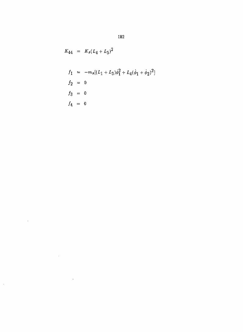
102

•^44 ~ K s { L ^ +

f l = — m s [ { L i + + 2 ) ^ ]

/2 = 0

/3 = 0

/4 = 0

103

PART II.

FORMULATION OF EQUATIONS OF MOTION FOR

RIGID/FLEXIBLE MULTI-BODY MECHANICAL SYSTEMS

104

CHAPTER 1. INTRODUCTION

Background and Motivations

A geometrically-constrained mechanical system is defined as an assemblage of

kinematic joints or geometric constraints and rigid/flexible links whose freedom of

motion is restricted to perform desired tasks. These diverse mechanical devices (i.e.,

machinery and vehicle systems) have moving parts that are geometrically-constrained

in some manner to transmit either motion or force to achieve design requirements.

In the past the design of mechanical systems was based on the assumption that

all links were rigid members. The equations of motion for a specific problem were

derived, programmed and numerically integrated. Recently, general purpose com­

puter simulation programs have been developed which automatically generate and

numerically integrate the equations of motion, and graphically display the simula­

tion results. Similar progress has been achieved for dynamic analysis of structural

problems undergoing small linear elastic motion. In this case, linear dynamic mod­

els are automatically formulated through the finite element method and solved with

modal analysis and linearized dynamics techniques. Typically, mechanical systems

composed of rigid bodies have a small set of highly nonlinear dynamical equations

with associated algebraic geometric-constraint equations because of the changing of

system configurations. On the other hand, dynamics of elastic structures are often

105

represented by a large number of degrees of freedom in the model.

Recently, the flexibility of mechanical systems has become one of the major con­

cerns of the system designers. The links of the mechanical system (e.g., robot arms,

mechanisms, vehicle structural components) are actual flexible structural members.

The operation of the mechanism may generate large external loads and inertial forces

acting on the members, which often results in a dynamic amplification of the link's

deflection and internal stress to the point where the system performance is degraded,

and even fatigue failure may occur. Hence, accurate and efficient analytical mod­

els which include the effects of distributed mass and elasticity are necessary for the

design of mechanical systems for greater performance.

The purpose of this work is to develop a computational methodology to pre­

dict and to optimize the dynamic response of geometrically-constrained mechanical

systems composed of rigid and flexible links. This methodology may be incorpo­

rated into an existing generalized mechanisms simulation formulation so that it is a

versatile design technique.

Literature Review

Dynamic analysis of a geometrically-constrained mechanical system includes a

series of steps: (1) the identification and classification of open or closed loops, (2)

application of dynamic principles to formulate the system equations of motion, (3)

the selection of coordinate frames to represent the moving part of the system, (4)

development of modelling techniques to include the flexibility efl'ects, and (5) refining

the solution technique and the graphic display of the simulation results.

106

Dynamic principles used to formulate system equations of motion

Significant work has been done in the formulation of dynamic equations of mo­

tion for open-loop, rigid-body spatial mechanisms and manipulator arms with various

modeling techniques and analytical mechanics principles [1-4]. Hollerback [5] devel­

oped a recursive procedure to formulate the system dynamic equations of motion

based on the Lagrangian approach, which was shown by Silver [6] to be equivalent to

the Newton-Euler method. Featherstone [7] developed another recursive algorithm

involving the quantities called articulated-body inertias. The kinematics of an open-

loop system were determined forward from the fixed ground link to the open end,

and the inertia properties of the system and the equations of motion were determined

backward with the application of the Newton-Euler principle.

Andrews et al. [8] developed a vector-network formulation technique for dy­

namic systems with kinematic constraints by using the Newton-Euler principle. This

method applied linear graph theory and built a library of different elements and

constraints. The determination of dependent and independent coordinates were not

included for closed loop mechanical systems so that the application of the algorithm

was limited to a set of simply constrained open-loop mechanical systems.

Kane and Faessler [9] used Kane's dynamic equations to conduct the dynamic

analysis for robots and manipulators involving closed loops. The independent gen­

eralized speeds were picked up by inspection according to the degrees of freedom

and the configuration of the system. Dependent generalized speeds were expressed

in terms of the pre-selected independent generalized speeds by using the geometric

constraint equations. The equations of motion were formulated consistent with the

number of degrees of freedom for the system. The solutions of the differential equa-

107

tions were used in the geometric constraint equations to determine the total system

dynamic response. This approach generated the minimum set of differential equa­

tions. The selection of independent speeds was done based on the understanding of

the mechanical system and the previous experiences of the analyst. This method

provided a systematic way of formulating the minimum number of system dynamic

equations by hand. The application of this method to formulate the general purpose

computer simulation program for dynamic analyses of closed-loop mechanical systems

was difficult because of the involvement of intuitive thinking and direct inspection in

picking up the subset of independent speeds.

Chace and Smith [10] showed that the elimination of variables from a set of non­

linear system equations was often prohibitively difficult. A whole set of generalized

coordinates, that had a much larger number than the system degrees of freedom, was

used in their formulations. Additional geometric constraint equations were used to

relate the dependent and independent coordinate variables. Orlandea et al. [11] used

a sparsity-oriented approach to the dynamic analysis of geometrically-constrained

mechanical systems. The dynamic equations of motion were established by using

Lagrange's equations and Lagrange multipliers in such a manner as to achieve max­

imum matrix sparsity. A stiff integration algorithm was developed which had the

capability of solving a simultaneous set of differential and algebraic equations.

Notation selections

Different notations have been used to represent the motion and forces of a me­

chanical system. Three dimensional vectors were used by Nielan [12] to represent

the translational and rotational motion of a body. The equations of motion were

108

formulated symbolically by using vector-dot-product operation according to Kane's

equations.

Woo and Freudenstein [13] applied screw coordinates to conduct dynamic anal­

yses of mechanisms. A three dimensional vector was represented by its direction and

magnitude. Yang [14] used the dual vector to analyze the inertia forces of spatial

mechanisms. Featherstone [7] used a 6 x 1 vector to represent the spatial translational

and rotational quantities in formulating the system dynamic equations.

Uicker [15-16] developed a unified modeling scheme by extending the Denavit-

Hartenberg (D-H) 4x4 matrix which treated the mechanical joints and rigid links

through the same transformation matrices with different translational and rotational

variables. Sheth and Uicker [17] further improved this method by defining two rele­

vant coordinate systems independently instead of using a common perpendicular axis

for two relevant coordinate systems.

Modelling of flexible mechanisms

The dynamics of flexible spatial mechanical systems have been studied by intro­

ducing flexibility efl'ects into the formulation of the system dynamic equations. The

nonlinear nature of the problem due to the changing geometry of the system proves

to be nontrivial [18]. The early researchers tried to solve the problem by considering

the dynamics of mechanisms separately from the response of the individual members.

The dynamics of the mechanisms were considered first with the assumption that the

members could be considered rigid. Once the motion and forces were determined

from rigid body dynamics, they were used as the input to the individual members

modelled by finite element method. The total response of each member is determined

109

by combining rigid body motion with elastic deflections [19-27].

Most researchers that followed formulated the equations of motion for flexible

mechanisms in coupled forms. Likins [28-29] discussed the hybrid coordinate ap­

proach in which separate coordinates were used to describe the large gross rigid-body

motion and the small flexible deflection.

Singh et al. [30-31] developed a computer simulation program for large mechan­

ical systems in a topological tree structure by using assumed displacement modal

functions to model the elastic body deformation in the system. The equations of

motion were formulated starting with Newton's law for a chosen mass particle in the

system. The scalar equations of motion were formulated by using vector manipula­

tions as used in Kane's equation approach.

Wielenga [32] formulated the equations of motion for a single flexible body and

compared the results with the dynamic equations of a single rigid body. The higher

order terms were eliminated by comparing two sets of the equations. The system

equations of motion were formulated by using the geometric constraint functions.

Buflinton [33] discussed the formulations of dynamic equations of motion for a

beam moving over supports by imposing kinematical constraints on an unrestrained

beam. This method modelled the manipulator arms with highly elastic members

directly related to the rigid support by using the assumed mode shape functions.

The interactions among flexible bodies as experienced in most open-loop mechanisms

were not included.

Ryan and Kane [34] and Ryan [35] derived the dynamic equations of motion for

a general beam attached to a rigid base by using assumed mode shape functions.

An irregularly shaped beam was used in the model and three dimensional beam

110

deflections were considered. This work primarily dealt with the motions of flexible

bodies directly connected to the moving rigid body. The flexible appendages do not

move through the arbitrary gross motion found in industrial spatial mechanisms and

manipulators.

Judd and Falkenburg [36] introduced the elastic deformation matrix to model

an open-loop multibody mechanical system. The deformation of a straight beam

was represented by a 4 x 4 transformation matrix. The equations of motion were

formulated by Lagrange's equation. The elastic vibrational motion was ignored in

determining the system kinetic energy based on the assumption that the elastic de­

flection is small compared to the large joint motion. This method considered the

elastic deflection of a flexible member only in the computation of the kinematics.

The coupling terms between the rigid body motion and the elastic deflection of the

link were omitted and only the beam bending mode was involved in the formulation.

Following the recursive formulation of dynamic equations of motion for rigid-

body systems proposed by Hollerback [5] and using 4x4 transformation matrix,

Book [37] developed an algorithm for recursive Lagrangian dynamics of flexible ma­

nipulator arms. This work provided an efficient and conceptually straightforward

modeling approach. The deflection of a link was represented in terms of a summa­

tion of mode shape functions. Only rotational joints with a single degree of freedom

were used in the formulation and the elastic link in the system was limited to a

straight-line beam, which may not be the case for a general open-loop mechanical

system.

I l l

Dynamics of closed-loop flexible mechanisms

Song and Haug [38] presented a general approach for dynamic analysis of closed-

loop flexible mechanisms. A body-fixed coordinate system was employed for each

element. Two sets of generalized coordinates representing the location and orientation

of a body-fixed reference coordinate system and the elastic deformation relative to

the body reference system were used. Geometric constraints were defined to impose

constraints between adjacent elements and the Lagrange's multiplier technique was

employed to incorporate the constraint forces.

Substructuring methods have been used extensively to reduce the number of

coordinates in dynamic analyses of structures. One category for substructuring was

based on the definition for a set of independent coordinate variables (master vari­

ables). The remaining coordinate variables (slave variables) were eliminated by dy­

namic or static condensation [39-40]. Another category for substructuring was based

on the selection of the partial modes or component modes [41]. The latter method

was found to be more attractive than the anterior one, due to the fact that master

variables must be chosen with care; otherwise, some of the lower frequencies in the

eigen-spectrum might be lost.

The mode superposition approach has been widely used in structural dynam­

ics [42-43]. Maddox [44] presented a method permitting one to truncate higher modes

in a dynamic sense, allowing smaller time step size, while the solution was represented

by the sum of lower mode dynamic responses.

Sunada [18] used perturbation coordinates to describe the small elastic motion

of the links from a prescribed nominal position. A 4 x 4 transformation matrix was

used to model the large displacement motion of mechanical joints. The finite element

112

method was used to generate the time independent mass and stiffness matrices for

each of the elastic members. The dynamic equations of motion were determined for

each link in terms of the perturbation coordinates. The large displacement geomet­

ric motion was assumed to be known either from the time history of the rigid body

simulation or from commanded joint prescription in servo controllers under the as­

sumption that the actual position of the manipulator was never very far away from

its command position. Compatibility matrices were used to assemble the individual

member equations into the system equations. The total system vibrational behavior

was obtained from the numerical solution of the system differential equations. This

study was limited to the rotational joints only. The mechanical system was treated as

a structure with different known configurations determined from the large displace­

ment motion of the mechanical joints. A general finite element program was used

to generate the mass and stiffness matrices that allowed a large selection of element

types. Some convenience and versatility, however, were lost due to the dependence

upon a large finite element program for computing the element mass and stiffness

matrices.

Turcic et al. [45-47] applied the finite element approach to study the dynamics

of elastic mechanical systems. Several coordinate systems were used to represent the

members in the system. Besides an inertia coordinate system located in an arbitrary

position, a rotational coordinate system located at the same origin was adopted to

represent the orientation of the body coordinate system fixed in a general point on

the undeformed link containing the finite element of interest. The dynamic equations

for each element were formulated in terms of the node displacements measured in the

body coordinate system. The equations of motion for each link were assembled in

113

the same way as in structural dynamics. The system dynamic equations were finally

formulated by using the transformation matrices, which were known from the large

displacement motion of the joints. An iterative integration technique was used to

solve the system dynamic equations. This method is essentially the same as that for

structural dynamics, except for the involvement of the large displacement geometric

motion in determining the transformation matrices for each link in the system. The

influence of large displacement geometric motion on the small elastic motion was

included, but the influence of small elastic motion on the large displacement geometric

motion was not included since the system dynamic equations were expressed in terms

of the elastic node deflection coordinates, while the geometric motion was included

only in the inertia force terms.

Shabana [48-52] and Shabana and Thomas [53] made a significant contribution to

the analysis of inertia-variant flexible multi-body systems. The configuration of each

flexible body was represented by two sets of generalized coordinates: reference and

elastic generalized coordinates. Reference coordinates were used to define the location

and orientation of a body fixed coordinate system. Elastic generalized coordinates

were used to represent the vibrational motion of each node in the body as used in

a finite element method. A Boolean matrix was included to impose the constraints

between adjacent elements, and the Lagrange's multiplier technique was used to

account for constraint forces between adjacent links. The modal analysis technique

was used to eliminate the insignificant modes of vibration. The final system dynamic

equations of motion were expressed in terms of the rigid body coordinates and flexible

body deformation coordinates with the use of Lagrange multipliers to incorporate the

geometric constraint forces. The dynamic response was obtained by the numerical

114

solution of both differential and geometric constraint equations. Agrawal [54] and

Agrawal and Shabana [55-56] extended Shabana's work by applying a mean-axis

notation to the dynamic analysis of flexible mechanisms. The mean-axis condition

was determined by minimizing the kinetic energy of the flexible body. The dynamic

equations of motion were formulated from the Lagrange equation approach with the

use of Lagrange multipliers to incorporate the geometric constraint forces. Because

of the involvement of Lagrange multipliers, the dimension of the system dynamic

equations had to be enlarged, and more computation time was needed to obtain the

total system dynamic response.

Dimension reduction of closed-loop mechanisms

To improve the computational efficiency, several methods have been proposed

to determine a set of independent coordinate variables, out of the total system co­

ordinate variables, so that the system dynamic equations could be reduced to the

minimum number subjected to the geometric constraint equations.

Wehage and Haug [57] developed an algorithm to identify independent and de­

pendent generalized coordinates by using a LU factorization of the constraint Jaco-

bian matrix. In this approach, nonlinear holonomic constraint equations and differ­

ential equations of motion obtained from the variation of Lagrange equations were

written in terms of a maximal set of cartesian generalized coordinates. A Gaussian

elimination algorithm with full pivoting was used to decompose the constraint Ja-

cobian matrix, to identify the dependent variables, and to construct an influence

coefficient matrix relating variations in dependent and independent variables. This

method started with the formulation of the dynamic equations at full dimension. The

115

Jacobian matrix was determined separately and was used to reduce the size of the

system dynamic equations.

Geometrically constrained mechanical systems were studied by comparing dif­

ferent approaches in reducing the dimension of the problem [58]. The first approach

was based on the selection of the independent generalized speeds. The geometric con­

straint equations were used to represent the dependent generalized speeds in terms

of the independent generalized speeds. The generalized active and inertial forces

were determined corresponding to the independent generalized speeds. The other

approaches utilized the singular value decomposition (SVD) of geometric constraint

equations. A closed loop mechanical system was first broken into an unconstrained

tree structure; then the equations of motion for this modified system were formulated

using Kane's equations. The geometric constraint equations for the original system

were obtained by using the SVD method.

Mani and Haug [59] also used a singular value decomposition (SVD) technique

in determining the solution of mixed differential-algebraic equations for dynamic and

design sensitivity analysis of geometrically-constrained mechanical systems. The dy­

namic equations of motion were written in terms of a maximal set of cartesian coordi­

nates to facilitate general formulation of kinematic and design constraint and forcing

functions. The operation of a SVD on the system Jacobian matrix generated a set of

composite generalized coordinates that were best suited to represent the system. The

total system coordinate variables were partitioned into a set of independent variables

and a set of dependent variables. After the integration for only the independent

coordinates, the total system response was determined through geometric constraint

equations from known independent variables.

116

Liang and Lance [60] applied a difFerentiable null space method to determine the

dynamic response of geometrically-constrained mechanical systems. The equations

of motion and geometric constraint equations were first formulated separately. La­

grange's multipliers were used to augment the dynamic equations. A continuous and

differentiable basis of the constraint null space was automatically generated by us­

ing the Gramm-Schmidt process on the system geometric constraint equations. The

independent coordinates were obtained by transforming the physical velocity coordi­

nates to the tangent hyperplane of the constraint surface. This method started with

the full dimension of the system. The final dimension of the system was obtained by

the transformation process.

Wampler et al. [61] and Wang and Huston [62] used Kane's equation to construct

the equations of motion for geometrically-constrained mechanical systems. The dy­

namic equations of motion for an open-loop mechanical system were formulated,

which consisted of the same number of bodies and the same configuration as of the

original closed-loop system except that the closed-loop was deliberately broken at

a chosen joint. The geometric constraint equations were constructed for the closed

system and were used to determine the relationship between the independent and

dependent coordinate variables. The dynamic equations were then reduced to the

minimum size (same as the number of system degrees of freedom) by substituting the

dependent coordinate variables for the independent coordinate variables. The system

total response was determined by integrating the differential equations and solving

the geometric constraint equations.

Several other methods were also developed to solve the combination of the system

differential equations and geometric constraint equations [63-66]. Most of the studies

117

on the geometrically-constrained mechanical systems were conducted by separately

formulating the system differential equations and geometric constraint equations.

Undetermined multipliers or Lagrange multipliers were used to augment the systern

dynamics equations. Several decomposition methods were used to reduce the size

of the equations to the number of the system degrees of freedom. The system to­

tal response was determined by solving the differential equations and the geometric

constraint equations.

A different approach to study the geometrically-constrained mechanical systems

was used by Sheth [67], Sheth and Uicker [68] and JML Research, Inc. [69]. In this

approach, the mechanical system was geometrically studied before the formulation

of the system dynamic equations. The degrees of freedom for a general mechanical

system were determined by manipulating the system geometric constraint matrix

so that this method could be used to handle the systems with various degrees of

freedom at different configurations. The independent coordinates were selected from

the total system coordinates by using the maximum mechanical advantage index

criterion. The Lagrange equation approach was used to formulate the minimum

number of system equations of motion corresponding to the independent coordinates.

Because the independent coordinates were selected before setting up the differential

equations, the minimum set of differential equations were formulated directly and

solved numerically, and the system total response was determined by solving the

system geometric constraint equations from known independent coordinate values.

118

Objective and Approach

The objective of this study is to build upon the past work on the dynamic analysis

of rigid-body mechanism systems to formulate system equations of motion for both

open and closed-loop rigid/flexible mechanical systems. These equations could be

used to develop a computational methodology for dynamic analysis of geometrically-

constrained, articulated rigid/flexible mechanical systems.

The 4x4 transformation matrix is used to model kinematic joints and link shape

matrices. Modal analysis techniques are used to incorporate the flexibility effects into

the link shape matrix. A three dimensional elastic deformation matrix representing

the deformation of flexible links is incorporated into the 4x4 rigid link shape matrix.

The mechanical system is mathematically modelled by the constraint relationships

and link shape matrices.

For open-loop mechanical systems, there are no closed-loop connections from

one reference link through kinematic joints and other links back to itself. Each joint

constraint variable is independent. The equations of motion corresponding to the

joint constraint and modal variables are derived by extending Book's work [37] with

the introduction of a general elastic deformation matrix, which is represented by the

summation of mode shape vectors and modal displacements so that irregular shape

flexible links in the system can be modelled. Another extension of this study is to use

a general kinematic joint constraint matrix to model different joint types. The recur­

sive formulation of system equations of motion is used to develop a computational

algorithm for dynamic analysis of open-loop mechanical systems.

The geometrically-constrained mechanical systems may include one or more

closed loops; therefore, the system degrees of freedom are less than the total number

119

of the joint variables. This study utilizes Sheth's kinematic analysis results [67] in

determining the independent oriented loops and system degrees of freedoms. The

relationship between dependent and independent kinematic joint constraints are ob­

tained through the iterative position analysis procedure. The minimum number of

system equations of motion are formulated corresponding to the independent joint

constraint and modal variables. The coupling effects between large displacement

geometric motion and small magnitude vibrational motion are included in the formu­

lation so that the simulation accuracy could be improved over the previous studies.

120

CHAPTER 2. GENERAL MODELLING CONCEPTS

A unified approach to the study of generalized, articulated mechanical systems

is significantly enhanced by a manipulative symbolic notation which contains the

essential parameters for a complete system description (Sheth [67]). The motions

and forces are vector quantities associated with designated kinematic joint coordinate

systems. The manipulation of these vectors requires the consideration of both the

magnitude and orientation of each vector in a common coordinate system, which is

often called the global coordinate system fixed in inertial space. The local or body

coordinate system is often used to describe the relative quantities within a body of

interest.

4 x 4 T r a n s f o r m a t i o n M a t r i x M e t h o d o l o g y

The 4x4 transformation matrix methodology for kinematic analysis was first

introduced by Denavit and Hartenberg in early 1950s, and was later generalized

by Uicker and Sheth [68]. The concept is to represent the vector relationships in

different local coordinate systems through a unified matrix notation. The absolute

position vector of a point is represented by a transformation matrix relating the local

coordinate system to the global coordinate system with the position vector of the

same point defined in the local coordinate system.

Figure 2.1: Representation of a position vector

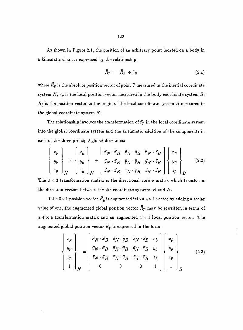
122

As shown in Figure 2.1, the position of an arbitrary point located on a body in

a kinematic chain is expressed by the relationship:

R p — R f j + r p (2.1)

where R p is the absolute position vector of point P measured in the inertial coordinate

system iV; rp is the local position vector measured in the body coordinate system B;

Rf^ is the position vector to the origin of the local coordinate system B measured in

t h e g l o b a l c o o r d i n a t e s y s t e m N .

The relationship involves the transformation of rp in the local coordinate system

into the global coordinate system and the arithmetic addition of the components in

each of the three principal global directions:

'

xp H

y p > = i

Vb • +

. 'P . N . ~~h . N

X p

i y p

. ' P

(2.2)

B

X N • V B • - B

V N • ^ B V N - V B V N ' %

% - ^ B % • V B ~ N • %

The 3x3 transformation matrix is the directional cosine matrix which transforms

t h e d i r e c t i o n v e c t o r s b e t w e e n t h e t h e c o o r d i n a t e s y s t e m s B a n d N .

If the 3x1 position vector Rf^ is augmented into a 4 x 1 vector by adding a scalar

value of one, the augmented global position vector Rp may be rewritten in terms of

a 4 X 4 transformation matrix and an augmented 4x1 local position vector. The

augmented global position vector Rp is expressed in the form:

(2.3)

X p % • ^ B ^ N ' V B X N • % H X p

y p y j Y • ^ B V N - V B y N • % V b <

y p

Z p % • ^ B % • y B % • % - b Z p

1 N

0 0 0 1 1 B

123

or in a symbolic matrix form:

R j , = [ T ] r p (2.4)

The 4x4 transformation matrix [T] is expressed as:

1T) =

where [T]^ is the 3x3 direction cosine matrix which represents the orientation of the

l o c a l c o o r d i n a t e s y s t e m w i t h r e s p e c t t o t h e g l o b a l c o o r d i n a t e s y s t e m ; [ T ] ^ i s t h e 3 x 1

translational vector which represents the location of the origin of the local coordinate

system measured in the global coordinate system; [0] is the 1x3 null row vector

that is combined with the scalar value of 1 to form the last row of the augmented

transformation matrix. The 4x4 transformation matrix contains all the information

necessary to describe an arbitrary point in one coordinate system with respect to

another system.

Kinematic Joint Transformation Matrix

The characteristics of a kinematic joint are modelled by the relative motion

between two adjacent links and their attached local coordinate frames. The relative

displacement for joint j, as shown in Figure 2.2, is expressed in the form:

' j ' = l ^ i Q j n ) ] '

y j

1 1

where is the 4 X 4 joint constraint transformation matrix, which relates the

relative large displacements (i.e., translation and rotation) at joint j between the

[T)r [T](

[0] 1 (2.5)

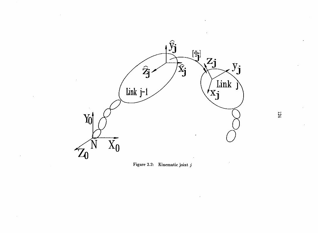
Figure 2.2: Kinematic joint j

125

two local coordinate systems [ x j y j Z j ) and ( x j y j Z j ) fixed on links j - 1 and j ,

respectively. The joint variable, qjj^, represents the relative joint displacement. The

number of joint variables may vary from one to six depending upon the number of

r e l a t i v e d e g r e e s - o f - f r e e d o m ( D O F ) f o r t h e j o i n t j .

For example, a cylindrical joint, as shown in figure 2.3, allows two independent

relative motions: (1) relative rotation and (2) relative translation. The two coordinate

systems attached to the adjacent links are defined in such a way that the rotational

axis is common to both systems. The relative rotation and translation of one joint

coordinate system (xjyjZj) with respect to the other one (xjyjZj) are measured by

the relative rotational angle {6) and the relative displacement (5), respectively. The

relationship between the two local coordinate systems is expressed in terms of the

joint variables (i.e., d and 5):

cos 9 — sin 0 0 0

h sin0 cos# 0 0 <

y j

0 0 15

1 0 0 0 1 1

Other kinematic joint types are formulated in a similar procedure. Detailed descrip­

tions of the kinematic joint types may be obtained from references [67-69].

Rigid Link Shape Matrix

The joint coordinate frames are appropriately located on each link of the kine­

matic chain. The relationship between two joint coordinate systems, which are lo-

Figure 2.3; Cylindrical joint

to a-i

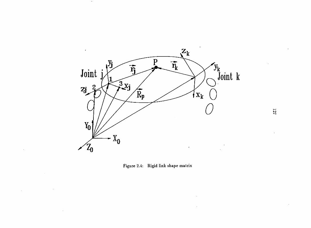
û 0

Joint k

to

Figure 2.4: Rigid link shape matrix

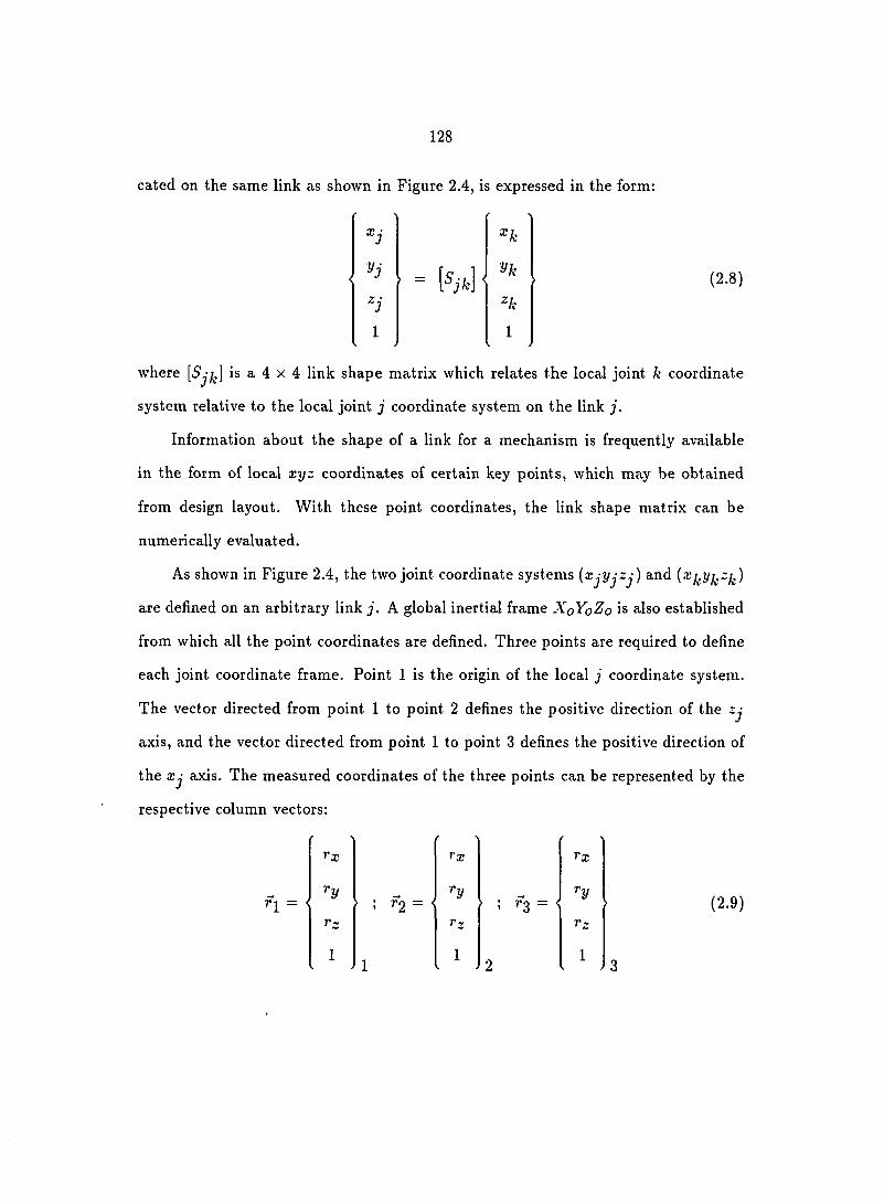
128

cated on the same link as shown in Figure 2.4, is expressed in the form:

• = K'd" V k

^ k

1 1

(2.8)

where [Sjj^] is a 4 X 4 link shape matrix which relates the local joint k coordinate

s y s t e m r e l a t i v e t o t h e l o c a l j o i n t j c o o r d i n a t e s y s t e m o n t h e l i n k j .

Information about the shape of a link for a mechanism is frequently available

in the form of local xyz coordinates of certain key points, which may be obtained

from design layout. With these point coordinates, the link shape matrix can be

numerically evaluated.

As shown in Figure 2.4, the two joint coordinate systems {xjyjzj) and

are defined on an arbitrary link j. A global inertial frame XQYOZO is also established

from which all the point coordinates are defined. Three points are required to define

each joint coordinate frame. Point 1 is the origin of the local j coordinate system.

T h e v e c t o r d i r e c t e d f r o m p o i n t 1 t o p o i n t 2 d e f i n e s t h e p o s i t i v e d i r e c t i o n o f t h e z j

axis, and the vector directed from point 1 to point 3 defines the positive direction of

the xj axis. The measured coordinates of the three points can be represented by the

respective column vectors:

n =

r x r x r x

r y • ; f 2 = < ^2/ II

r z r z r z

1 1

1 1 1 2

(2.9)

129

The vector forms the last column of the transformation matrix, which relates

the origin of the local coordinate system x j y j z j to the global coordinate system

XoYqZo. The first three columns of the transformation matrix, [T^j], represent the

u n i t v e c t o r s a l o n g x j , y j , a n d z j a x e s , r e s p e c t i v e l y , a s d e f i n e d i n t h e g l o b a l XQYOZO

coordinate system. The transformation matrix, [T^j], is expressed as:

[ T o j ] =

' •

X I ^2 ®3 r x

h n n < > < > < y < >

h :2 h r z

0 0 0 1 3 3 3 3 .

(2 .10)

The unit vector along the x j axis is determined through the normalized vector

relationship between points 3 and 1:

^1

h

-1

0

Z3-fl

\/(^3 -n) (^3 -^i) (2 .11)

Similarly, the unit vector along the z j axis is determined through the normalized

vector relationship between points 2 and 1:

^3

n

-3

0

r2 - r i (2.12)

The unit vector along the y j axis is determined by the cross-product operation be-

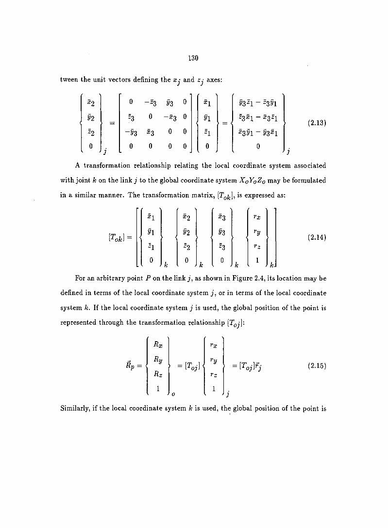
130

tween the unit vectors defining the xj and zj axes:

H

n

^2

0 j

0 0 0 n 0 X I ygzi - 2391

^3 0 -X3 0 <

n . — <

^3®1 - H h

- n ®3 0 0 h ^3^1 - n n

0 0 0 0 0 0

(2.13)

A transformation relationship relating the local coordinate system associated

with joint k on the link j to the global coordinate system XQYOZO may be formulated

in a similar manner. The transformation matrix, is expressed as:

[^ofc] =

•

XI X 2 ®3 r x

h #2 m ^2/ < > < > < ' < >

h ^2 ^3 r z

G G 0 1 . k k k k .

(2.14)

For an arbitrary point P on the link j , as shown in Figure 2.4, its location may be

defined in terms of the local coordinate system j, or in terms of the local coordinate

system k. If the local coordinate system j is used, the global position of the point is

r e p r e s e n t e d t h r o u g h t h e t r a n s f o r m a t i o n r e l a t i o n s h i p [ T ^ j ] :

Rp =

Rx r x

R y ^2/

Rz r z

1 1 > < 0 » '

= [ T o j ] r j (2.15)

Similarly, if the local coordinate system k is used, the global position of the point is

131

represented through the transformation relationship

Rx rx

Ry

II ^2/

Rz rz

1 0

1

(2.16)

The link shape matrix, relates the local coordinate systems x j^y f^z j^ to x jy jz j

at each end of the rigid link and is obtained by combining Equations 2.15 and 2.16

to form the relationship:

rj =

rx

^2/

rz

rx

^2/

rz

1

(2.17)

Through this modelling procedure, the appropriate point data are used to deter­

mine the rigid link shape matrices for all links in the mechanism before any elastic

deflections occur.

Flexible Link Shape Matrix

There has been an increasing interest in the incorporation of structural flexi­

bility effects into the dynamical equations of rigid link systems. The most widely

used methods for studying flexibility include the finite element method, experimen­

tal modal analysis, and component mode synthesis. The technique of finite element

analysis has been extensively used for structural dynamics, but is often difficult to

use for large displacement dynamic analysis of mechanical systems because of the

132

changing of system geometry. Modal analysis procedures are useful in evaluating dy­

namic characteristics of large mechanical systems. The finite element method can be

used for any.particular elastic body in the system to formulate the equations of mo^

tion. Eigensolution techniques are used to determine the mode shapes of vibration.

Typically, a few mode shapes corresponding to the lower frequencies can be used to

approximate the flexibility of the link. Assumed elastic mode shape functions are also

used to approximate the vibrational characteristics of the link. In this formulation

procedure, the elastic deformation of a point in the mechanism is approximated in

the form; mj

(2.18) 4 = Z k=l

where dj is the approximation of the elastic deflection at any point on the link

measured in the local coordinate system with m.j modes of vibration being used;

^i) is the fcth mode shape vector which is a function of the location of the

point of interest within the link; is the A:th modal variable of the link i which

represents the magnitude of the fcth vibrational mode at time t .

To simplify the procedure of formulating the dynamic equations of motion, one

may model the elastic link as a set of discrete points or nodes. The modal displace­

ment of the tth vibrational mode of link i at the node g is expressed in the form:

^ikg

^ikg

0

(2.19)

By mode superposition, the approximated elastic deformation, d^g, at node g of link

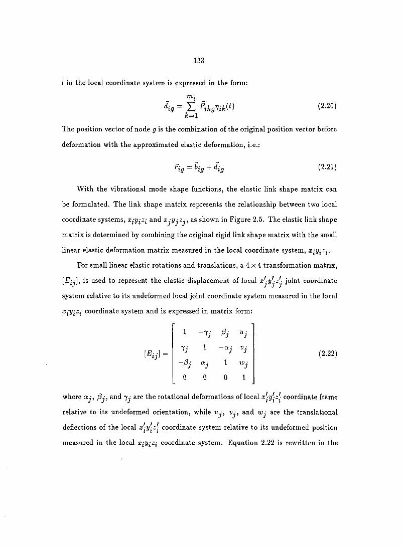
133

i in the local coordinate system is expressed in the form:

mz

^ig k=l

(2.20)

The position vector of node g is the combination of the original position vector before

deformation with the approximated elastic deformation, i.e.:

^ig = hg + (2.21)

With the vibrational mode shape functions, the elastic link shape matrix can

be formulated. The link shape matrix represents the relationship between two local

coordinate systems, and xjyjzj, as shown in Figure 2.5. The elastic link shape

matrix is determined by combining the original rigid link shape matrix with the small

linear elastic deformation matrix measured in the local coordinate system, x^y^z^.

For small linear elastic rotations and translations, a 4 x 4 transformation matrix,

[Eij], is used to represent the elastic displacement of local joint coordinate

system relative to its undeformed local joint coordinate system measured in the local

coordinate system and is expressed in matrix form:

[Eij] =

1 -Tj

Tj 1

1 W j

0 0 0 1

(2 .22)

where aj, l3j, and jj are the rotational deformations of local x'^y'^z'^ coordinate frame

relative to its undeformed orientation, while wy, vj, and Wj are the translational

deflections of the local coordinate system relative to its undeformed position

measured in the local x^y^z^ coordinate system. Equation 2.22 is rewritten in the

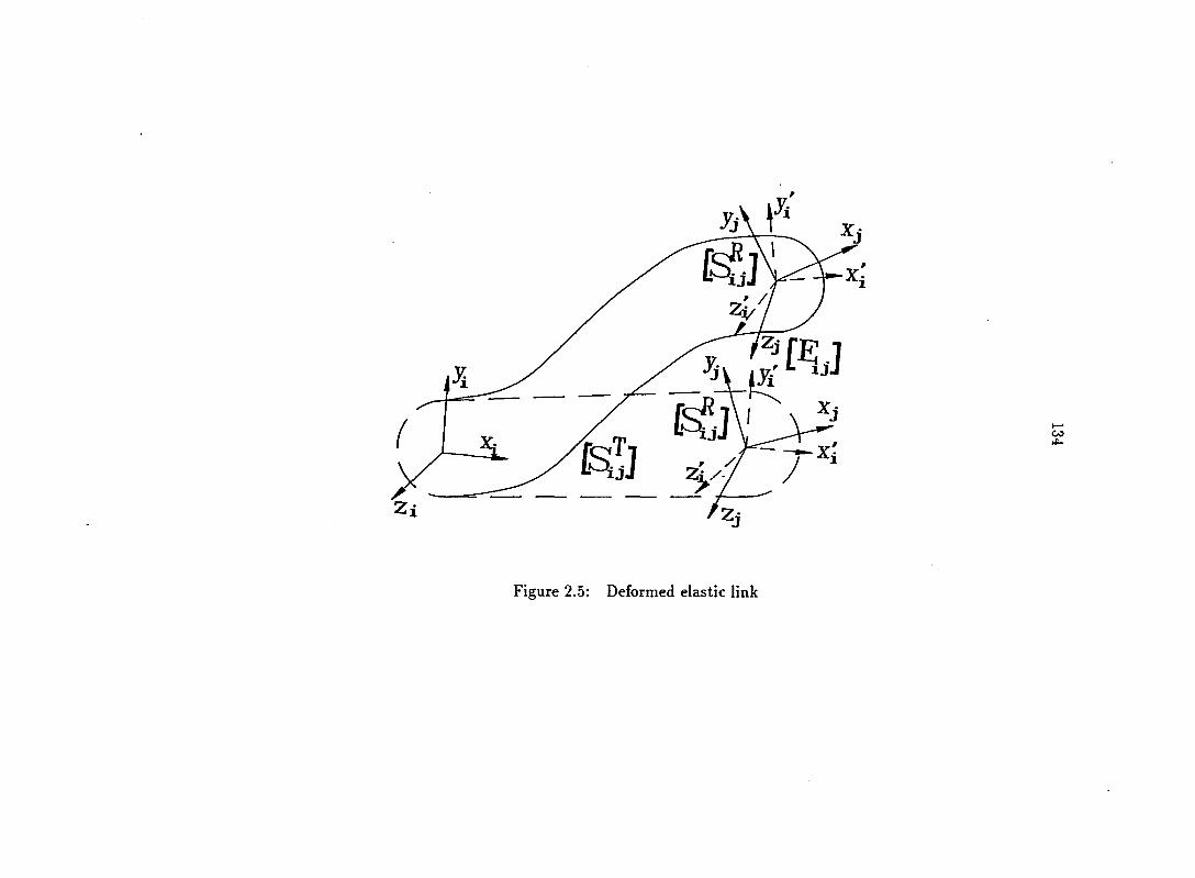
Zi

Figure 2.5: Deformed elastic link

135

form: mi

(2.24)

l^ijl = M + E tihmiHikj] (2-23) &=!

where Viki^) is the A;th modal variable of the link i; [7] is the identity matrix; [H^f^j]

is the tth mode shape at the origin of the local XjyjZj coordinate system. Matrix

is expressed in terms of the modal displacements at the origin of joint j

coordinate system in the form:

® ~^ik6 ^ikb ^ikl

Pike 0 -Pik4: Pik2

-Pikb Piki 0 ^ikZ

0 0 0 0

where {I = 1,2,...,6) is the kth mode shape at the origin of the local XjijjZj

coordinate system on link i. The first three elements (i.e., in this tth

modal matrix represent the modal translational deflections while the remaining three

elements (i.e., represent the rotational deflections about the and

zi axes of the imaginary local joint coordinate system, respectively.

For link flexibility, the rigid link shape matrix is rewritten in the form:

i^ikj] =

1%1 = IsSlls.fl (2.25)

where matrix [5^^] defines the translational position of the imaginary parallel coor­

dinate system relative to the local joint i coordinate system and is expressed

in the form:

1 0 0 zv

\SÏj\ = 0 1 0 y;

0 0 1 ZI

0 0 0 1

(2.26)

136

Matrix [S^] defines the angular orientation of the local joint j coordinate system

relative to the local joint i coordinate system and is expressed in the form:

(2.27)

0 0 0 1

The elastic link shape matrix is formulated by combining the rigid body shape

matrix with the small linear deflection matrix. The formulation of flexible link shape

matrix for an arbitrary link is conceptualized as three successive events: (1) the rigid

body translation of the joint j local coordinate system relative to the joint i local

coordinate system, (2) the linear elastic deformation of the link, and (3) the rigid

link angular orientation of joint j local coordinate system relative to the joint i local

coordinate system and is expressed in the form:

The linear elastic deflection matrix, [E^j], adjusts the deformed displacement (i.e.,

translation and rotation) of the joint j local coordinate system relative to its unde-

formed position of the joint j local coordinate system. For rigid links, the matrix

Kfl = (2.28)

[E^j] becomes the identity matrix and the elastic link shape matrix has the same

form as for rigid link shape matrix, as shown in Equation 2.25:

|s| l = islj \{s§] = [SijI (2.29)

137

CHAPTER 3. DYNAMICS OF OPEN-LOOP MECHANICAL

SYSTEMS

Kinematic Analysis of Open-Loop Mechanisms

The kinematic model of a mechanism requires the mathematical description of

the kinematic joints which constrain the relative motion between adjacent links. The

transformation matrices for the links and joints are assembled to form the kinematic

chains, either open-loops, closed-loops, or a combination of both open and closed-

loops. The motion of a link or a point on the link of interest is studied through the

kinematic models.

Position of a given point

Through the 4x4 transformation matrix relationships for joint constraints (i.e.,

Equation 2.6), rigid link shapes (i.e.. Equation 2.8) and flexible link shapes (i.e..

Equation 2.28), the absolute position of a point P on the link i is determined by

consecutive transformation operations. The local position vector, Fp, locates the

position of point P on link i. The global position vector, Rp, is expressed in terms

of the relative joint and link transformation matrices in the form:

Rp = (3-1)

138

where [$] is a joint transformation matrix and [5] is a link shape matrix in a kinematic

open-loop mechanism.

The absolute position vector, Ap, is written in terms of an abbreviated general

transformation matrix and a local position vector:

-Rp = (3-2)

where is the general transformation matrix and is defined as:

[^oi] = l'5'l2^2'5'23^3-'^i-l,i^i (3-3)

Equation 3.3 involves all the joint and modal variables between the global coordinate

system and the ith local coordinate system.

Velocity of a given point

The absolute velocity of a point P on link i in a mechanism is determined by

the time derivative operation on the absolute position vector (i.e., the first derivative

of Equation 3.2 with respect to time):

= + oFp (3.4)

For rigid links, the distance between any two arbitrary points within the link is

constant (i.e., the relative velocity is zero). For flexible links, the relative motion

of a point measured relative to a local coordinate system is not equal to zero. The

relative velocity is a function of modal velocities and the relative point location.

The time derivative of the general transformation matrix, is determined

in terms of the joint and modal variables for all the joints and links from the fixed

139

global inertial frame to the link of interest and is expressed in the form:

i _ , i-1

[^oil ~ X] •^o,h—l^h'^hi X/ ^oh^h,h+l'^hi h=l h=l

where

[\h-l] = ^1^12^2%-%-l,/:

[\i] = ^h,h+^^h+l-^i-l,i^i

= ^hMl^hi

l^oh] = ^1^12^2%"A-1,A*A

~ •^o,h—l^h

[%i] = ^h+l^h+lM2-^i-hi^i

~ ^h+l-^h+l,i

(3.6)

(3.7)

(3.8)

(3.9)

It is noted that [Âoo] is an identity matrix.

The time derivative of a joint constraint matrix is computed by considering each

of the joint variables and is expressed in the form:

{^h\ = 5$,

. % 1 .

= E a=l

%i + .ag&2.

%2 + - + %iV, /iJ

(3.10)

where is the ath joint variable of the joint h. This general procedure allows

different joint types to be used in the formulation.

140

The partial derivative of the joint constraint matrix with respect to the joint vari­

ables (i.e., ) is performed by the matrix pre-product operation of a derivative

operator on the joint constraint matrix. For example, the derivative of the cylindrical

joint constraint matrix with respect to the rotation angle (i.e., = 9) is expressed

in the form:

— sin 0 — cos 0 0 0

L%1

cos I

0

0

— s i n 0 0

0 0 0

0 0 0

= Qhl^h (3.11)

The derivative operator matrix, [Q/,],], is obtained in the matrix form:

3*6

[%lJ (3.12)

For this particular joint, the derivative operator matrix, [Q/ji]? corresponding to the

rotation variable (0) is expressed in the form:

IQhl] =

0 - 1 0 0

1 0 0 0

0 0 0 0

0 0 0 0

(3.13)

Similarly, the derivative operator matrix, corresponding to the translation

variable (5) is expressed in the form:

\ .Qh2\ =

0 0 0 0

0 0 0 0

0 0 0 1

0 0 0 0

(3.14)

141

The first derivative of the cylindrical joint constraint matrix with respect to time is

expressed in the form:

\ .^h\^Qhl^h^ + Qh2^h^ (3-15)

For a given joint type, these derivative operator matrices are determined with

respect to each joint variable and need only be computed once. This same procedure

is used to develop a simulation program's library for different joint types and the

derivative operator matrices.

The time derivative for flexible link shape matrix is computed in the form:

d ' jP R [*^/i,/i+l] - ^ ^h,h+l^h,h+l^h,h+l

cT p cR h,h+l^h,h+l'- h,h+l (3.16)

The derivative of the elastic deflection matrix /i-j-l] is expressed in terms of the

modal velocities of link h:

= E Vhl3^hl3 (3.17) f3=l

where is the /9th modal velocity of the link h\ is the /3th elastic mode

shape of link h at the origin of the joint h+1 coordinate system. rp

The translational part of the shape matrix of link h, [Sj^ the angular

orientation part of the shape matrix, are known from the rigid body shape

matrix in Equation 2.25.

The first derivative of the general transformation matrix, as expressed in Equa­

tion 3.5, is rewritten in terms of the joint constraint and modal velocities:

i

~ E Xj ^o,h—lQha'^h—l,i^ha É (3.18) /i=la=l /i=l/3=l

142

where

= ^ohSh,h+'^ (3 19)

= slh+l^u (3.20)

Numerical values for Equations 3.19 and 3.20 are computed once the particular link

of interest and its relative position are known.

The relative velocity of node g on the link i is approximated by mode shapes

and modal variables in the form:

mi

^ig = 'J2 PiagVia (3-21) a=l

The absolute velocity of node g on the link of interest is expressed explicitly in

terms of the time derivatives of the joint and the modal variables, as expressed in

Equation 3.4, and is used to compute the system kinetic energy functions.

Acceleration of a given point

The formulation of system equations of motion requires the explicit expression

of the acceleration of a given point P on the link of interest in the open-loop system.

The acceleration of the point P is determined by performing the time derivative

operations on the velocity function of the same point, as expressed in Equation 3.4:

~ ^oi^V + + oFp (3.22)

The second derivative of the general transformation matrix with respect to time,

[Aqj], needs special attention because it includes explicitly the joint and modal ac­

celeration terms. The second derivative of matrix, with respect to time is

[^oi] d

dt

143

computed from Equation 3.18 in the form:

i _ i-1

h=\ ^ h=lfi=l

i _

~ XI ^o,h—\^ha^h—\,i^ha h=l «

i-1 ^ + E E Kh^hjSHmjB + (3 23)

/t=l /3=1

where is the ith acceleration remainder which includes all the terms in

except the terms and 7/^^. The second time derivative of the joint constraint

matrix is expressed in the form:

The acceleration remainder, is expressed in the form:

[^ri] ~ ^r,i—l^i ^^o,i—l^i -'^Oji—1 XZ oT iia^ijS (3.25) a=1/3=1

The second time derivative of the elastic link shape matrix is expressed in the form:

A,/t+l] = E (3.26) /?=1

The acceleration remainder, is expressed in the form:

[•^/•,i—ll ~ ^r,i—I'^i—l,i ^•^o,i—I'^i—l,i (3.27)

Equations 3.25 and 3.27 are computed recursively.

The computational process of the acceleration remainders for the first few flexible

links in an open-loop mechanical system is illustrated. The general transformation

144

matrix, contains only the first joint constraint matrix with Ni joint variables:

Mol] = ^1 (3.28)

The acceleration remainder, includes the cross products of all velocity terms:

^1 ^1

The general transformation matrix from the global inertial frame to the end of the

first link, includes the first joint constraint and link shape matrices:

Moll = ^1-^12 (3.30)

The acceleration remainder, is determined in the form:

[l^l] = + 2iol'^12 (3.31)

The general transformation matrix from the global inertial frame to the second joint

of the system includes and the second joint constraint matrix and is expressed

in the form:

[•'^o2\ = ^1-^12^2 = ^ol^2 (3.32)

Similarly, the acceleration remainder, [^^2], is determined in the form:

N2 #2 ^2^ [^r2l = ^rl^2 + 2^01^2 + ol Z! I] —ô^92a92/3 (3,33)

a=l^=l

With these known forward recursive formulae for acceleration remainders, the equa­

tions of motion are formulated in terms of generalized joint and modal variables

through the application of the system energy functions.

145

Generalized Dynamical Equations for Open-Loop Mechanisms

Two types of variables are used to describe the system motion characteristics:

(1) the joint variables to describe the large displacement geometrical motion; (2) the

elastic modal variables to approximate the small elastic vibration of the link of interest

about its original rigid link configuration. The equations of motion corresponding to

joint constraint variables are formulated by using Lagrange's method in the form;

d (dKE\ _ dKE , dPE _ p.

a = 1, 2, . . . ,

i = 1, 2, ...,% (3.34)

where is the ath independent variable of joint i; is the generalized nonconser-

vative force corresponding to the virtual displacement . The equations of motion

corresponding to modal variables are formulated by using Lagrange's method in the

form:

d (dJŒ\ _ OKA I dPE _ r* ^ \ ^Via / ^Via la

a = 1, 2,

i = 1, 2, ...,n (3.35)

where is the ath independent modal variable of the flexible link of interest; F*^

is the generalized nonconservative force corresponding to the virtual displacement

The equations of motion involve the partial and total derivative operations on

the kinetic and potential energy functions with respect to each of the independent

joint and modal variables. The kinetic and potential energy functions and their

146

derivatives, as required in Equations 3.34 and 3.35, are computed in the following

sections.

System Kinetic Energy Function

The kinetic energy of a link is computed by summing the kinetic energy at each

discrete mass particle in the link. The total system kinetic energy is obtained by

summing the energy terms for each link in the system.

The velocity of node g on the link of interest (i.e., link z) is expressed in the

form:

Kg = Rig = Ki^g + King (3-36)

The kinetic energy of the link of interest is computed by summing all the kinetic

energy terms at every node within the link and is expressed in the form:

KEi = E , (3.37) 5=1

where iVGj is the total number of the nodes in the link of interest; Tr[A] is the trace

operator on a matrix, [A], and is expressed in the form:

Tr[A] = (3.38) i=l

The trace of a transposed matrix (i.e., Tr[A^]) has the same value as the trace of the

original matrix (i.e., Tr[A]), which is defined as the arithmetic sum of the diagonal

elements of the square matrix and yields a scalar value.

Substituting Equation 3.36 into Equation 3.37, the kinetic energy of the link

of interest is written in terms of general transformation matrix, and the first

147

derivative of general transformation matrix, the local position and velocity

vectors of a node on the link of interest and is expressed in the form:

= 2 ^ (3.39) 5=1

It is convenient to define some intermediate terms in the kinetic energy function.

The general transformation matrix, and the first derivative of the general

transformation matrix, remain constant for each node of the link of interest.

The first intermediate term, [Jj], contains the local position vectors of all nodes in

terms of the original rigid body position and the elastic deformation for each node of

the link of interest and is expressed in the form:

[ J i ] = E "^igng^Jg (340) 5=1

The second intermediate term, contains the local position and velocity vectors

of all nodes on the link of interest in terms of the modal displacements and velocities

and is expressed in the form:

= Z ^ig^g^ig (3-41) 5=1

The third intermediate term, contains the local velocity vectors in terms of

the modal velocities for the link of interest and is expressed in the form:

= Z ^ig^g^g (3.42) 5=1

Using these intermediate terms, the kinetic energy for the link of interest is rewritten

in the general form:

KEi = ^-Tr (3.43)

148

The kinetic energy for the entire system is computed by summing the kinetic energies

for each link in the open-loop system and is expressed in the form:

n 1 -Tr

i = l ^ (3.44)

From the kinematical analysis, it is found that the first derivative of the gen­

eral transformation matrix, [A^^], involves the time derivatives of both the joint and

modal variables for all joints and flexible links between the global inertial coordinate

system and the local coordinate system on the link of interest. After substituting

Equation 3.21 into Equation 3.42, the intermediate term, expressed explic­

itly in terms of the modal velocities for the link of interest in the form:

mi

a=l (3=1 (3.45)

IZ ^ig^iag^ii3g (3.46)

where a and /? are the subscript variables representing the ath and /9th modes,

respectively. The 4x4 matrix, has zeros for the entries in the last column

and row and is expressed in the form:

NGi

E 5=1

where is the equivalent mass at the node g of link i; Pjag is the ath mode shape

at the node g of link i. The matrix, is determined from the pre-determined

mode shapes for the link of interest and remains constant during the simulation.

The expression for the matrix, [Jjq,], in Equation 3.41 is rewritten in terms of

the modal displacements and velocities and is expressed in the form:

m:

K'a) = E Via a=l

m,-

^ia X/ Vij3^il3a. /3=1

(3.47)

149

where is the coupled inertia term between the rigid body position and the

elastic mode shapes of all nodes on the link of interest and is expressed in the form:

NGi

ICial = Z ^ighg^ag (3-«) 9=1

Equation 3.40 involves the local position vectors which are determined by com­

bining the rigid body position and elastic deflection vectors at each node for the link

of interest and is expressed in the form:

mi mi mi

[ J i ] = Q + Z Viai^ia + ïa) + Z Z maVi(3<^ia(3 (349) Q=1 a=l (3=1

where [C'J is the original rigid body mass distribution for the link of interest and is

expressed in the form: NGi

K-i'] = Z ^ighg^g (3-50)

With these defined variables, the system kinetic energy is explicitly related to

the joint and modal variables. The derivatives of system kinetic energy with respect

to both joint constraint and modal variables are obtained from the kinetic energy

functions as expressed in Equation 3.44.

Kinetic Energy Function Derivatives

The formulation of the system dynamical equations with Lagrange's approach

requires the derivatives of the system kinetic energy function with respect to the

independent generalized variables of the system. The derivative operations of the

system kinetic energy function with respect to the large displacement joint variables

are conducted in the first subsection while the second subsection deals with the

150

derivative operations of the system kinetic energy function with respect to the modal

variables.

Derivative of kinetic energy with respect to a joint variable

For an open-loop mechanical system, the joint variable, and its velocity,

qj^, appear in the kinetic energy functions for links from j through ti, as shown

in Figure 3.1. The general transformation matrix, is a function of the joint

and modal variables for all the joints and flexible bodies between the global inertial

Coordinate system and the local coordinate system for the link of interest (i.e., l ink i).

The first derivative of the general transformation matrix with respect to time,

includes the joint displacements and velocities, as well as the modal displacements

and velocities of the flexible links. The partial derivative of the kinetic energy with

respect to the ath independent velocity of the jth joint (i.e., qj^) influences all links

from link j to link n in the open-loop kinematic chain and is expressed in the form:

dKE = t \ T r

l=J

^j.\T

(3.51) H j a

The general transformation matrix, [-4^^], does not include the joint velocity

terms, so that the derivative of the matrix, with respect to the joint velocity,

(jjQ,, is zero. The trace of the first term on the right hand side of Equation 3.51 is

equal to the trace of its transpose which is expressed in the form:

Tr dq ja

= Tr (3.52)

o Link

o

Cn

Figure 3.1: Representation of an open-loop mechanism

152

With the relationship expressed in Equation 3.40, the traces of the first and second

terms on the right hand side of Equation 3.51 are identical because the link inertia

matrix, [J^], is symmetric. These two terms are combined into one term. It is also

noted that time derivative operations on both numerator and denominator can be

simplified to the form; T/îi -1 \ f ) A • '

(3.53)

The general transformation matrix, [^4^^], is a continuous function of the independent

variables and time. The derivative operations may be switched without changing the

final value as expressed in the form:

/i . M ,i . (3.54)

' d

dt \^1ja) _ 9qja_

Substituting Equations 3.52 and 3.53 into Equation 3.51, the partial derivative of

kinetic energy with respect to is expressed in the simplified form;

dKE n

^'ija dq 3 a dq J a (3.55)

The time derivative of Equation 3.55 is expressed in the form:

d dKE n

dt \dqjc, i=j

OA

dqja ' j o t

+ 01 dqja ^Ijoc

T \T (3.56)

For the second term in Equation 3.34 for Lagrange's method, the partial derivative

of the kinetic energy with respect to a generalized joint displacement (i.e., g^^) is

153

expressed in the form:

dKE n a,;. = Ê&ÎTjT , ^ T

oi

dA^; dA„: J.4 . /., 2i 4- 01

Jikl^ 01 (3.57) ^ j a """ija

Subtracting Equation 3.57 from Equation 3.56 yields the first part of Lagrange's

equation corresponding to the derivatives of system kinetic energy functions with

respect to the joint displacements and velocities and is expressed in the form:

à dKE It [dqja

dKE

n E T r

t=j dq ja i^oi + (4 + ~ •^ik'l^oi + (•'i/t ~ •^ikO^oi) Z

cv 1? 2,..., iVj 1,2,...,??. (3.58)

In Equation 3.58, the intermediate terms, [J^-] and associated with the matrix,

[Â^-], contain the modal displacements and velocities of link i. Using Equations 3.47

and 3.49 and performing the time derivative operations, these intermediate terms are

expressed in terms of the modal velocities in the form:

mi

Ji + ik - Jik = 2 ^ Mk^ik k—1

(3.59)

where matrix, is the newly defined term which is a function of the mode shapes

and modal displacements for the flexible link i and is expressed in the form:

rm; ' ,T = IC'itl + E

./=1 (3.60)

where is the mass distribution due to the rigid body position and the flexible

mode deflection of all mass particles within the flexible link i, as defined in Equa-

154

tion 3.48; inertia matrix, [Cn^i], is the mass distribution due to the flexible mode

deflections of all mass particles of the link i as defined in Equation 3.46.

The intermediate terms associated with the matrix, [-4^-], in Equation 3.58 are

expressed in terms of the modal accelerations for the link i in the form:

mj

[^ik - 4w] = Z Vik^ik (3-61) k=l

With Equations 3.59 and 3.61, Equation 3.58 is rewritten in terms of the general

transformation matrix and its time derivative, and the modal velocities and acceler­

ations for the link i, in the form:

d (dKE\ _ dKE _

n Y,T t i=j

a,t / "'i ^ •g 44 + 2 E mhOik-ili + E mkDikA i

\ k=l k=l y

a = 1, 2, ..., Nj; j = 1, 2, ..., n (3.62)

Equation 3.62 represents the system kinetic energy partial derivatives with respect

to each of the joint displacements.

Derivatives of kinetic energy with respect to a modal variable

The modal displacements of flexible link j appear in the kinetic energy functions

for link j through n, as shown in Figure 3.1. The modal displacement, of

link j influences all the bodies from j+l to n through the general transformation

matrix, in Equation 3.3, and influences itself through the intermediate terms

in Equations 3.40 - 3.42.

155

The partial derivative of the system kinetic energy with respect to the modal

velocity, is expressed in the form:

^ = E Tv i=j+l

Ê&i J.ÀT, , Mm oz

+Tr d J j ^

Sljn

+ l^oj ' d J ^ u jkl

(3.63)

The first part of the right-hand side of Equation 3.63 is associated with the bodies

following the link j while the second part expresses the influence of on itself. The

intermediate term, [Jj], in Equation 3.40 includes only the modal displacements. The

partial derivative of the term, [Jj], with respect to the modal velocity, Vj^i is zero.

The time derivative operation on Equation 3.63 is expressed in the form:

£ ( it

n = E Tr

i=j+l

dA

ai,j0 I 01

+

+ dA

dA,

oz

+ Tr

+A,

Siljis

 'dJ. jk

oj

a?;/) '

aL + A,

01

OJ

' d J j k \ - T 1 -A

OJ

(3.64)

For the second term in Equation 3.35 for Lagrange's approach, the partial derivative

of kinetic energy with respect to the modal displacement, Vjf3^ is expressed in the

156

form:

= y Tr dA

ni3 + Ak^ii

dAr

dA^: 01 + dA 01

01

4- Tr 'a. d j ^

àL + A, dj. jk

(3.65)

Subtracting Equation 3.65 from Equation 3.64 yields the first part of Lagrange's

equation corresponding to the derivatives of system kinetic energy function with

respect to the modal displacements and velocities, and is expressed in the form:

d IdKE\ _ dKE _ Tt ^

n .E Tr i=j+l

dA ^ + (4 + Jik ~ •^Fk'l^oi + (jik - JikO^m)

+Tr 'oj (s^f ) ^oj + Aoj (g^ "oj

d " M \ A (3.66) y3t~d^

The first part of the right-hand side of Equation 3.66 is associated with all the links

following link j due to the influence of the modal displacement, and has the

same form of the terms as expressed in Equation 3.58 where the derivatives of system

kinetic energy function with respect to joint variables, qj^, are concerned. The

157

second part on the right hand side of Equation 3.66 deals with the motion of link

j corresponding to the modal displacement, Vji3- The derivative operation of the

intermediate terms with respect to the modal variable, VjfSi a^nd the modal velocity,

is expressed in terms of the mode shape functions. The partial derivative of

[Jj/j] with respect to the modal velocity, is expressed in the form;

d mj rtij

E + E njicjui) k=l 1=1 TTl'

= + E = ^jl3 k=l

(3.67:

The second term in the second part of Equation 3.66 is expressed in terms of the

modal, displacements in the form:

\ d J , L d j ^ 7r^-5;p-

mj

~ '1(3 + ^ E "^jk^^'JfSk - jl3k) «=1

(3.68)

Again using the matrix property that the trace of a matrix equals the trace of its

transpose, as expressed in the form:

Tr = Tr (3.69)

the second term in the second part of Equation 3.66 becomes zero. The third term in

the second part of Equation 3.66 is simplified by performing the appropriate deriva­

tive operations on the intermediate terms as shown in Equations 3.40 - 3.42 and is

expressed in the form:

158

TH.;

= 2 E Vjk<^ji3k k=l

(3.70)

The fourth term in the second part on the right-hand side of Equation 3.66 is ex­

pressed in terms of the modal accelerations in the form:

r r i j

= Z %k(Cjl3h + (3-71) k=\

i

dt dvjis

After substituting Equations 3.67 - 3.71 into Equation 3.66, the first part of La­

grange's equation corresponding to the derivatives of system kinetic energy with

respect to the modal displacement and velocity is expressed in the form:

d I B K e] _ d K E _

n E Tr

i=J + l

dA mi mi

dv 2 \ 2 E ik^ik-^oi E ik^ikA . \ k=l k=l

T oi

r / +Tr

mj

^oj^jl3 + E ^jk^'j0k E ^jk^'jfSk ) ^oj . \ A:=l k=l

System Potential Energy Function

mj nT (3.72)

The system potential energy consists of both the potential energy due to gravity

effects and the flexible link strain energy. The potential energy due to gravity is

determined by considering each mass particle at node g for the link of interest and

is expressed in the form:

PE9 = -Y: 1=1 ^=1

(3.73)

159

where R^g is the absolute position vector of the mass particle, mig, for the link of

interest; G is the absolute acceleration of gravity vector and is expressed in the form:

G — [gxi gyi gzi 0] (3.74)

After substituting the expression for the absolute position vector Rig, as expressed

in Equations 3.2 and 2.21, the potential energy due to gravity is expressed in the

form:

PE9 = Y. Tt i=l g=l

mi

a=l

n = - Y . T r

i=l

mi

a=l (3.75)

where the term, [Bj], is associated with the potential energy due to the rigid body

mass distribution and is expressed in the form:

NG4 ^ (3.76) [-®il = z

5=1

The term, is associated with the potential energy due to the flexible link mass

distribution and is expressed in the form:

NGi (3.77)

5=1 ^ig^iag^

The elastic potential energy of the system is expressed in the form:

PE' = Z Udif lKi\{di} i=l

(3.78)

where {dj} is the nodal elastic displacement vector for the link of interest; [A'j] is the

stiffness matrix for the link of interest and is computed with a finite element analysis

160

program. The nodal displacement vector is approximated by a few mode shapes and

the modal variables and is expressed in the form:

mi (4) = Z! ViaiPia) (3-79)

q:=1

where is the ath modal variable for the link of interest; is the ath mode

shape vector for the link of interest. Substituting Equation 3.79 into Equation 3.78,

the scalar value of the system elastic potential energy is expressed in the form:

1 n = 2 E E E (3-80)

i=rl a=l /3=1

The term, is computed by using the mode shape vectors and the stiffness

matrix for the link of interest and is expressed in the form:

^ial3 = (381)

The system potential energy is expressed in terms of the joint and modal variables

of the open-loop system.

Potential Energy Function Derivatives

The system potential energy consists of both the potential energy due to grav­

ity effects and the elastic strain energy. The elastic strain energy is a function of

the nodal displacements of the link and is approximated by the mode shapes and

modal displacements. The partial derivative of the strain energy with respect to

joint displacements is zero and is expressed in the form:

dpEe

161

The partial derivative of the potential energy due to the gravity with respect to the

joint displacement is expressed in the form:

The partial derivative of the potential energy due to the elastic deformation with

respect to the modal displacement is expressed in the form:

The elastic deformations change the system configuration and contribute to the sys­

tem potential energy due to gravity. The partial derivative of the potential energy

with respect to the modal displacement is expressed in the form:

System Dynamical Equations for an Open-Loop Mechanism

After substituting the partial and total derivatives of the system kinetic and po­

tential energy functions with respect to the general joint displacements and velocities,

the modal displacements and velocities, and time, the system equations of motion

are obtained by Lagrange's formulation.

The equations of motion corresponding to the joint displacement (i.e., qja) ^-re

obtained by substituting Equations 3.62, 3.82 and 3.83 into Equation 3.34 and are

expressed in the form:

dPE9 (3.83)

(3.84)

T' (3-86)

162

( X — 1 , 2, N j ] j — 1, 2, . . . , 7 1 (3.86)

The equations of motion corresponding to the elastic modal displacements (i.e.,

VjjS) 3^re obtained by substituting Equations 3.72, 3.84 and 3.85 into Equation 3.35

and are expressed in the form:

Equations 3.86 and 3.87 are the governing dynamical equations for an open-loop

mechanical system composed of both rigid and flexible members. It is difficult to

use these equations directly because they are written in terms of the transformation

matrices which contain implicit functions of the independent variables. A simula­

tion algorithm, however, may be developed from these two sets of the generalized

governing system equations.

r / m • rrij \

l3 — 1, 2 , . . . , TTijJ j — 1, 2 , . . . , n (3.87)

163

CHAPTER 4. DYNAMICS OF CLOSED-LOOP MECHANICAL

SYSTEMS

Kinematic Analysis of Closed-Loop Mechanisms

Due to the existence of geometric constraints and the requirement that the

closed-loop mechanism remains connected during its range of prescribed motion, the

system degrees-of-freedom (DGF) are less than the total number of the joint con­

straint variables. Mathematically, the interconnected assembly of links and joints

is represented by a set of algebraic equations in which the geometric compatibility

must be satisfied for the complete range of prescribed motion. The formulation of

these constraint equations is based on the identification of independent loops, which

is inherited from the mechanical design.

Sheth [67] successfully applied linear graph theory,to systematize the manipula­

tion of the topological characteristics of an arbitrary closed-loop, rigid-body, geometrically-

constrained mechanical system. An algorithm to identify an oriented, optimum set

of constraint loops was based on the following four criteria: (1) the set must con­

tain all possible independent loops; (2) each loop must leave the fixed ground link

through a single designated constraint; (3) any two loop passing through the same

kinematic constraint (i.e., a joint) must do so in the same direction; and (4) the

distance around each loop must be the minimum achievable under the above con­

164

ditions. An numerical iterative position analysis determined the number of system

DOF and the relationship between the dependent and independent joint variables

at each design configuration of the mechanism (i.e., the topological characteristics).

The kinematic analysis (i.e., the computation of positions, velocities and accelera­

tions of system links and points of interest) was conducted for specified joint motions

(i.e., positions, velocities and accelerations). The independent variables were selected

from the collection of all system joint displacements and were based on the system

condition number, or the maximum mechanical advantage criterion.

The iterative position and kinematic analyses are adopted in this research project.

The link shape matrix is extended to include flexible link effects. The results from

the kinematic analysis are used to formulate the system dynamic equations of motion

for any geometrically-constrained, multi-link mechanical systems composed of both

rigid and flexible links.

Loop-closure position analysis

For a closed-loop mechanism, the closed form solutions for the dependent mo­

tion variables are formulated in terms of the independent variables. For a generalized

solution scheme, the dependent and independent variables cannot be pre-decided

because the total system DOF may change with the changing of the mechanism con­

figurations. A practical approach is an iterative technique in which initial estimates

are made for the solution results and successively better corrections are found from

linearized equations. This method was used by Sheth [67] for closed-loop, rigid-body,

geometrically-constrained, mechanical systems.

For a geometrically-constrained mechanical system with flexible links, this itéra­

165

tive scheme can also be applied to conduct the position analysis. For a given motion

condition, the flexible link will experience oscillatory elastic deformations. A flexible

link shape matrix includes the deflection information (i.e., the mode shape functions

and modal variables). The kinematic joint variables must be adjusted to assure the

assembling of the system. The elastic deformation does not alter the kinematic joint

DOF. The joint displacements are adjusted to satisfy the system constraint require­

ments while the link shape matrices are kept 'constant' at any design configuration.

The iterative position analysis for a constrained mechanical system assembles the

changing system configuration and determines the degrees-of-freedom at the design

configuration. The relationships between the dependent and independent constraint

variables are also determined by using the system geometric constraint matrix.

The initial estimate of the ith variable for joint j , is assumed available. The

true value of the variable at a given configuration is represented by an estimate and

a correction error term:

(lji = yi + Qji (4.1)

The geometric constraint matrix for the joint is approximated in the form;

( = l,2,3,...,iVj (4.2)

For a closed-loop mechanism with n geometric constraints, there is a closed

sequence of 2n coordinate frames fixed on either end of the individual links. Beginning

with the first joint coordinate frame on the ground link and applying consecutive

transformations, the loop closure equation for an arbitrary kinematic loop is written

in the form:

^ol^l'^12^2%^3-'^n-l,n^ri5„,lAio = I (4.3)

166

where [/] is the 4x4 identity matrix; [^4^^] and [A-^q] are the general transformation

matrices which relate the global inertial coordinate system to the first joint coordi­

nate system. The loop closure equation contains the rigid/flexible link shape and

joint constraint transformation matrices, and specifies that the mechanism forms a

closed assembly. Mathematically, the loop-closure equation provides a set of nonlin­

ear algebraic equations relating the joint constraints and elastic modal displacements

of the mechanical system, and is used for the kinematic analysis. For a multiple loop

mechanical system, there are as many loop-closure equations as there are independent

loops in the system.

The A independent loop-closure equations for the entire system are expressed in

the general forms:

^ol[^l'^12^2'5'23^3-'^n-l,n^n5'TOl]l^lo = I

^ol[^l '5 ' l2^2%^3-'^TO-l,n^n'5 'nl]2^1o =

^ol[^l'^r2^2%^3-*^M-l,n^n'-'^nl]/'4lo = I

^ol[^l'^12^2^23^3-'^n-l,n*n'5'„i];^/llo = / (4.4)

It is noted that the loop-closure equations contain different combinations of links and

joints for each of the independent loops. The joint constraint matrices are approxi­

mate while the link shape matrices are assumed to be known.

The first order approximation of the joint constraint matrix corresponding to

167

the estimation of the joint variable, is expressed in the form:

[*?] ^ [#7] + Ë i=l \

0$,

dq 6q

1ji=yiJ

(4.5)

where Nj is the total number of variables for the jth joint.

The partial derivative of the joint constraint matrix with respect to a joint

variable is represented by pre-multiplying the derivative operator matrix with the

= Q• Equation 4.5 is rewritten joint constraint matrix,

in the form:

I .e. ,

i=l

Nj

i—1 (4.6)

where [/] is the 4x4 identity matrix. Substituting the approximated joint constraint

matrix, as expressed in Equation 4.6, into the Ith. loop equation, the approximation

of the loop-closure equation is written in the form:

iVi N2

'?2i^î2z)^2-^23-i=l i=l

^3 _ Nn (^ + Y, Qni^^n i )^ ' r iS j i i ] iA io % I (4.7)

i=l i=l

Carrying out the matrix multiplications and ignoring higher order products, such

as Sqji^qmni Equation 4.7 for the Ith loop is linearized in the form:

^ol[^l'^12^2%^3-'^n-l,n^n*^nll/^lo

+^ol[(Zl<?li%j)^l'^12^2%^3"-^TC-l,n^n'^nl]/^lo

168

i

+^o1[^1'5'i2^2'^23(Ç Qzi^%i)^3-^n-l ,n^nSni]iAiQ i

+ • • • +

+Aoi [ ^ lS i2^2^2Z^3 - ^n - l , n iY ,Q n i ^1n i ) ^nSn l ] lA io % I (4.8) i

A term in Equation 4.8 is written in a general matrix product form:

An abbreviated notation for matrix multiplication is defined in the form:

i^oj] = ol^lSl2^2^23-^j-lSj-l , j (4.10)

Upon inserting the identity matrix, (i.e., I = after the term [Qj i ] in

Equation 4.9, it is rewritten in the form:

[('^oj^ji^oj 1 ]/^ 1 oi

= [KjQjiKj"\Moo)ikji

= [Bji]l{Âoo)lSqji (4.11)

where

I H ^ A i — f/4-.-O [Bji]i = [AojQjiÀ h (4.12)

Since the 3x3 rotational submatrices of [Aqj] and are always orthogonal and

the rotational submatrix of [Qj i ] is always antisymmetric, the matrix, [B j i ] , has the

169

general form:

[Bjih =

0 g^.^(l,2) Bj^(l,3)

g^.^(2,l) 0 gj^(2,3) B^,(2,4)

B^.^(3,2) 0 B^.,(3,4)

0 0 0 0

(4.13)

where the 3x3 submatrix in the upper-left corner of matrix, [Bjj], has the properties:

Bj^{m,n) = —Bj.i{n,m)\ m = 1,2,3; w = 1,2,3 (4.14)

The approximated loop closure equation for the /th loop, as defined in Equa­

tion 4.8, is written in the form:

ini = û ô } ) i - i (4.15) I

Ç + Ç B2i^l2i + •••• + Ç niK. . i i i

where the subscript i has the range from 1 to the total number of constraint variables

for each joint. Equation 4.15 is written in shortened form:

|£/I = ( ^ m ) / - / (4.16)

The variation of the joint variables is contained in the error correction matrix,

and is expressed in the form:

Y1 + IZ B2i6q2i + .. . . + m L I

(4.17)

When the /th constrained kinematic loop is closed properly, the error correction

matrix is equal to the 4x4 null matrix while the matrix, is equal to the

4 x 4 i d e n t i t y m a t r i x . D u r i n g t h e i t e r a t i o n p r o c e s s , t h e a p p r o x i m a t e d v a l u e s o f t h e

170

constraint variables are written in the general error correction matrix equation in the

form:

0 Ei{l,2) Ei{l,Z) E;(l,4)

0 EX2,4)

Ei{3,l) Ei{S,2) 0 Ei{3,A)

0 0 0 0

an - 1 «12 «13 ®14

«21 «22 - 1 «23 «24

«31 «32 «33 - 1 «34

0 0 0 0

(4.18)

It may be shown that there are only six independent elements in the matrix, [Ei\.

Six independent terms for the /th loop may be extracted from Equation 4.18 and

written in the form:

£^(l,4) = ai4

^/(2,4) = «24

£'/(3,4) = «34

£^(3,2) = «32

= «13

E/(2,l)=a2i (4.19)

These equations when combined with similar equations for the remaining loops may

be solved for the error corrections, ^Çjii as used in Equation 4.1. This process is re­

peated to obtain better and better approximations until the corrections are negligible.

171

[ifi' -^00 (4.20)

The matrix, [Ei], approaches the null matrix while the matrix, [Aqq], approaches

the following form:

ail ®12 0 0

0 «22 «23 0

(^31 0 «33 0

0 0 0 1

The rotational submatrix has the additional orthogonal property which results in the

following two conditions:

«11 ~ «22 ~ «33 ~ ^ (4-21)

and

«12 = «23 = «31 = 0 (4.22)

The matrix, has the following range of values after convergence:

{•Aoo)i - 1 (4.23)

± 1 0 0 0

0 ±1 0 0

0 0 ±1 0

0 0 0 1

In order to force the diagonal elements to converge to +1 and to speed up the iterative

procedure, the final form of equations for the correction terms of the Ith. constraint

loop is written:

£/(l ,4) = 014

-2^/(2,4) = 024

^/(3,4) = 034

^/(3,2) = 032 + 033 + 022-2

172

•2^/(1,3) = ai3 + «11 +033-2

Ei{2,1) = 021 + ®22 + «11 - 2 (4.24)

These equations contain all the variation terms of the joint variables in the /th loop.

The explicit equations for these unknown correction terms are expressed in the matrix

form;

^912

(1,4) ^12(1,4) . • -521(1,4) .

Bl (2,4) -512(2,4) . . ^21(2,4) . • ^niVn(2,4)

Bl (3,4) ^12(3,4) . • 521(3,4) . • ^R/VTi(3,4)

Bl (3,2) ^12(3,2) . . ^21(3,2) . • '5niVn(^'2)

Bl (1,3) -^12(1,3) . . 521(1,3) . • 5nA^n(l'3)

Bl (2,1) -^12(2,1) . . ^21(2,1) . • ^nyVn(2,l)

6921

ai4

«24

«34

«32 + «33 + «22 - 2

«13 + «11 + «33 - 2

«21 + «22 + «11 - 2

The total number of constraint variables in the /th loop is determined by simply

summing the number of constraint variables for each joint:

(4.25)

NJi

Z = 1 (4.26)

where NJi is the number of constraint joints for the /th loop; t I j is the number of the

173

joint variables in the ith joint. Equation 4.25 is written in condensed matrix form:

1^1,

Q X t i i / x l 6 x 1

It is noted that the vector, {5}, is used to represent the error correction terms,

with a one to one correspondence.

For a mechanical system with A independent loops, there are A matrix loop

closure equations which are solved simultaneously. The coefficient matrix, [7V]^ (/ =

1,2,...,A), is assembled to form a 6A x i system coefficient matrix. The correction

terms, (i = l,2,...,i), corresponding to each of the generalized joint variables is

also properly combined to form the {txl) vector of unknowns. Thus, the total system

loop closure equations are generated in the form:

(4.8, 6 A x f ( X 1 6 A x l

If there are s specified independent variables, (i = 1,2,...,5), the correction

terms for these variables are equal to zero. The generalized constraint variables,

(jj, (i = 1,2,have a one to one relationship with the joint variables which are

originally expressed by the double subscripts. The rearrangement of the columns in

the matrix, [#], makes the last s columns and the last s variables in the vector, {6}

, correspond to the specified independent coordinates. The number of the specified

independent coordinates is equal to or less than the total system DOF. Otherwise,

the mechanical system is over specified which violates the connected assembly re­

quirement.

The number of the independent equations depends on the rank of the coefficient

matrix, [N]. If the rank of the matrix is r, there are r independent equations.

174

The t — r constraint variables which are not solved from the geometric conditions

are called independent generalized coordinates and must be determined in order to

solve for the r dependent variables. The determination of the rank of the coefficient

matrix provides the number of independent equations and the total number of the

dependent variables. The system DOF are equal to the number of the independent

coordinates and are determined by subtracting the rank from the total number of

the constraint variables (i.e., DF = t — r). Since the matrix, [iV], accounts for all

special geometric characteristics of the mechanical system, this generalized method

determines the system DOF for any geometrically-constrained mechanical systems.

The determination of the rank r and the selection of the optimum r x r nonsingular

submatrix of matrix, [N], are accomplished numerically by a standard Gaussian

elimination technique with full pivoting.

The numerical operations on the geometric coefficient matrix, [#], result in the

partitioned matrix form;

[N\ = (4.29) [^Irxr ^^^rx{t-r)

l-^l(6A—r)xr [•^Î(6A—r) x (i—r)

where [G] is the r x r nonsingular square matrix; [C] is the (6A — r) x r general

matrix; [H] is the r x (t — r) general matrix; [/)] is the (6A — r) x {t — r) general

matrix. The Gaussian elimination technique interchanges the rows and columns of

the original matrix, [TV], except for the last s columns corresponding to the specified

constraint variables. The relative locations in the vectors, {i?} and {5}, are also

175

altered accordingly. The rearranged vectors are represented in partitioned form:

{^l}(rxl)

{ R } = (4.30)

and

{5} =

{^2}((6A-r)xl) .

{^l}(rxl)

(4.31)

G H f ^ i W < f = 1

C D [ « 2 J l

(4.32)

The first (t — r — s) elements in vector, {#2}, correspond to the additional independent

generalized coordinates, if any. The last s elements in vector, {^g}, correspond to

the specified independent coordinates. The partitioned matrix equation is written in

the form:

R2

The correction terms for the dependent variables in vector {6^} are computed from

Equation 4.32 in the form:

{'1} = (4.33)

The last s elements in vector, {62}, are zero because the correction terms for the

specified independent coordinates are not required. The correction terms for the first

{t — s — r) elements in the vector, {62}, may be arbitrarily selected. If they are also

selected as zeros, Equations 4.33 is simplified to the form:

{il} = |Gl-l{fli} (4.34)

The correction terms in vector, {^j}, are used to update the corresponding constraint

variables, qj^. The iterative procedure continues until a norm of {5]^} is less than a

176

predetermined tolerance, Thus, the mechanical system is assumed to be properly

assembled under the condition:

II 11< q (4.35)

Even though only r independent equations out of original 6A equations are used in the

final solution, all unused equations must be compatible and are checked by solving

the remaining equations in Equation 4.32, i.e.,

{i?2} = (4.36)

If this condition is not satisfied, the procedure informs the designer that the mechan­

ical system cannot be assembled in the design configuration by s specified indepen­

dent coordinates. The numerical test for the incompatibility is conducted by using

the vector norm defined in Equation 4.36, i.e.,

||{i!2}-|CK<i}||>£2 (4.37)

where eg is a predetermined small tolerance. When the condition set by Equation 4.37

is true, it is sufficient to indicate the incompatibility or the failure to assemble the

mechanism.

The geometric system equations and the submatrix, [G], play an important role

in determining the system DOF at any given design configuration. The numerical

procedure also selects the optimum set of free generalized independent coordinates,

(FG'C), from the system DOF, when a set of specified generalized independent co­

ordinates, (SGC), are prescribed.

177

First partial derivatives of dependent coordinates

The formulation of system equations of motion requires velocity information for

each dependent generalized coordinate, which is related to the velocities of the inde­

pendent coordinates. The system equations are written in terms of the generalized

independent coordinates. When the system is properly assembled by the iterative

procedure, the system loop-closure equations, which include both dependent and

independent constraint variables, are used to determine the partial derivatives of de­

pendent coordinates with respect to an independent coordinate for a given system

configuration.

For a properly assembled mechanical system, the constraint variable values are

exact. Therefore, the loop-closure equations are equal to the identity matrix. The

independent generalized coordinates are designated by qfj,{k = 1,2, ...,DF), which

are predetermined from the group of joint variables, qj^. The partial derivative of

the /th loop-closure equation with respect to a generalized independent coordinate,

% {k = 1,2,...,DF), is written in the form:

^{-4ol[^l5i2^2%^3-'^n-l,n^n5„l];Aio = /} (4.38)

Carrying out the derivative operations yields the following matrix equation:

+Aoi[$i5i2^523$3...5„_i,„$n5rii]/Aio

- t - > l o 1 [ $ 1 5 1 2 $ 2 % - 1 , n n 1 1 Z 1 0

+^ol(*1^12*2%^3""^n-l,R^'^nlWlo = [^1 (4-39)

The partial derivative of a joint constraint matrix with respect to an independent

178

generalized coordinate is expressed in the form:

r<9$ (4.40)

Using Equation 4.40 and the matrix, as defined in Equation 4.12, the first

partial derivative of the /th loop-closure equation with respect to the independent

generalized coordinate, %, is written in the form:

•

= [0] (4.41)

It is noted that matrix, [B j j ] , has only six independent terms for the /th loop.

Equation 4.41 is expanded in terms of the six simultaneous linear algebraic equations:

5ii(l ,4) ^12(1,4) . • ^21(1,4) . • ^nAr„(l'4)

5ii(2,4) ^12(2,4) . . ^21(2,4) .

Bii(3,4) ^12(3,4) . • -521(3,4) . • •8niV„(3,4)

Sii(3,2) Bi2(3,2) . . ^21(3,2) . - ^nArT,(3,2)

5ll(l ,3) 5I2(1,3) . • -821(1,3) . • •8niVn(l'3)

5ii(2,l) ^12(2,1) . • -821(2,1) . • ^niV„ (2>1)

> = <

0

0

0

0

0

0

(4.42)

The simultaneous linear equations for the entire system are assembled in the form:

(A'l |^}={0} (4.43)

where [N] is the system geometric coefficient matrix, as written in Equation 4.28.

The numerical computation procedure is the same as for the position analysis. The

matrix equation obtained from Equation 4.43 is written in partitioned form:

G H

C D

1%} {e&}

{0}

{0} (4.44)

179

where {e^} is a DFx 1 unit vector with all elements being equal to zero except the one

corresponding to the independent generalized coordinate, for which the derivative

has a value of one.

The solutions for the first partial derivatives of the dependent coordinates with

respect to the independent variables are obtained from Equation 4.44 in the form:

(4.45)

Since the matrices, [G] and [ H ] , are known from the iterative position analysis, no

additional computations are required to solve for the first partial derivatives.

Second partial derivatives of dependent coordinates

The second partial derivatives of dependent coordinates with respect to an in­

dependent generalized coordinate are obtained by differentiating the constraint loop-

equations twice. Differentiating Equation 4.41 with respect to an independent gen­

eralized coordinate, qm, yields the equation:

d

dq, 'm = [0] (4.46)

L I i I

The second partial derivatives of the /th loop-constraint equation with respect to the

independent generalized coordinates, qf^ and qm., are expressed in the form:

1:% '^dqkdqm dqi^dq '92* + .... + 2 ni

dqj^dqi + [C'(Â:,m)] = [0]

(4.47)

where

[C(k,m)] = Ç

L i

dBii dqii y dB2i dq2i dqm dqf^ ^ dqm dqf^

+ •••• + ^1n\i ^ dqm dqf^

(4.48)

180

A typical term,

[Bjj], in the form

dB 21

\dB

dqm

oqrn

d

, in matrix, [ C { k , m ) ] , may be computed from the matrix,

dqm

dA 03 dqm ^oj dq-m ^oj '^ ' '^ojQji dq: m

(4.49)

The partial derivative of the first term in Equation 4.49 with respect to the generalized

coordinate, qm, may be written in the form:

dÀ oj dq m dq m

[Aoi^lSi2^2^23--^j-l^j- l , j] = [^jmÂoj] (4-50)

where

w jmi (4.51)

The partial derivative of the second term in the Equation 4.49 with respect to the

generalized coordinate, qm, may be written in the form:

dq m

_ ; ^

a=l VVaj Sqm (4.52)

The partial derivative of the third term in Equation 4.49 with respect to the general

coordinate, qm, is computed from the identity matrix in the form:

'^ojAol = ojÂjo = I (4.53)

The derivative operation of Equation 4.53 is written in the form:

dqm dq "m (4.54)

181

The derivative of the third term in Equation 4.49 is expressed in the form:

'dÀ, dÀ-} oj dq. m

= -OJ dqm ^jo - ^oj '^jm (4.55)

A typical term in matrix, [C(fc,m)], may now be expressed in the form:

\dBji dqji] ^oj

a=l ^'Jja 9qm

dq i j i

^1k (4.56)

The six simultaneous linear equations for each loop may be formulated by the same

procedure as used in determining the first derivative equations, i.e.,

dqf^dqm

^qk^qm

Bl (1,4) ^12(1,4) . • ^21(1,4) . • 5niV„,(l '4)

Bl (2,4) ^12(2,4) . . ^21(2,4) . • B n N j 2 , 4 )

Bl (3,4) ^12(3,4) . . ^21(3,4) .

Bl (3,2) ^12(3,2) . . ^21(3,2) . • B^^^{Z,2)

Bl (1,3) ^12(1,3) . • 521(1,3) .

Bl (2,1) ^12(2,1) . • ^21(2,1) . . 57z7Vy,(2,l)

dqfjOqm

^ \Nn ^qk^qm

. m ] C'uik,:

C'24(A:,m)

C32(A:,m)

C i ^ { k , m )

C 2 i ( k , m )

(4.57)

182

The simultaneous linear equations for the entire system may be again assembled in

the form: ^

[N]\^-^] = -{C{k,m)} (4.58) dqf^dqm

res of 1

are equal to zero. The partitioned matrix equation from

The second partial derivatives of the last DF independent generalized coordi

, I 1 nates m vector

Equation 4.58 is written in the form:

G H <

C D

^2 izi. {C'i(fc,m)}

{ C 2 { k , m ) } (4.59)

{0}

The second partial derivatives for the dependent generalized coordinates with respect

to independent generalized coordinates are obtained in the form:

It is noted that matrix, [G], is available from the position analysis. The only numerical

computations needed for the second derivative terms are the formulation of the right-

hand side of Equation 4.58.

Dependent motion computation

The motion of a geometrically-constrained mechanical system is specified by the

motions of independent coordinates, SGC. The motions of the dependent generalized

coordinates are related to the motions of the independent generalized coordinates

through the geometric constraint equations.

A typical dependent geometric constraint variable, qj^, is a function of the in­

dependent variables, qj^,{k = 1,2,..., DF) which are selected in the position analysis

183

procedure. This relationship is written in the form:

= 9ji(9l,g2)93'-'9DF) (4-61)

The velocity of a dependent constraint variable, qj^, is a function of the independent

generalized velocities. The partial derivatives of the variable, qj^, with respect to

each of the independent variables are expressed in the form:

Equation 4.62 can be rewritten in matrix form:

where is a [ D F x 1) velocity vector of independent coordinate variables; | |

is a {DF X 1) partial derivative vector of qj^ with respect to each of the independent

coordinate variables as computed from Equation 4.45.

The acceleration of a dependent variable, qji, is obtained by the time derivative

operation on the velocity function in Equation 4.63 and is expressed in the form:

f 1 The time derivative of the vector, < >, is expressed in terms of the second partial

derivatives of the dependent coordinate variable with respect to each of the indepen­

dent coordinate variables as well as the velocities of the independent coordinates in

the form:

d j dqji 1 _ d'^qji . d^qji . ô'^qjj .

d t [ d q f ^ } ""

k = 1, 2, . . . ,DF (4.65)

184

Equation 4.65 is rewritten in matrix form:

-I dt \

a2 i j i

dqf^dqm

k = m = 1, 2, DF

{Q t u }

(4.66)

The acceleration of a dependent constraint variable, is then expressed in the

form;

dqfjdq; m {qm} (4.67)

After the independent coordinate motions and the first and second partial derivatives

are computed, the dependent coordinate motions are determined from Equations 4.63

and 4.67.

Velocity of a general point

From the iterative position analysis, the orientation of each independent loop

is already known. The velocity of a point on a rigid link is uniquely defined by the

motions of the constraint variables. The velocity of a point on a flexible link, however,

is determined from the combination of rigid body motion and the elastic deformation.

The velocity of modal displacements together with the mode shapes for the link are

used to approximate the velocity of a point on the flexible body.

The absolute position vector of node g is determined through the matrix loop

equation:

= KFIq (4.68)

where [A^^] is a 4 x 4 general transformation matrix. Even though the transformation

matrix, [A^^], includes all the joint constraint matrices from the origin of the global

185

inertial coordinate system to the link I, not all the constraint joint variables are

independent because of the existence of closed-loop constraints. The velocity of node

g is then expressed in terms of the velocities of the independent constraint variables,

which are determined from the system position analysis, and the modal velocities for

the link I and is expressed in the form:

The second term on the right-hand side of Equation 4.69 accounts for the flexibility

"effects. The distance between any two points on a rigid body remains constant in the

local coordinate system, thus the time derivative of the position vector is zero. For

flexible links, the elastic deformation causes small motion between two points in the

link, thus the time derivative of the local position vector is not equal to zero.

The time derivative of the general transformation matrix, [^q /], consists of the

velocities of the independent constraint and the modal variables of all rigid and

flexible links in the system. Because the magnitude of joint displacements is typi­

cally larger than that of the elastic deformations, the velocity of the link / may be

approximated by the independent constraint variables with the steady-state elastic

deformation of the flexible members being included in the modified link shape ma­

trices within the loop closure equations. The time derivative of matrix, is

expressed in the form:

It is noted that the partial derivative of the matrix, [A^^], with respect to a gen­

eral independent constraint variable, q^., may be determined in the same manner as

% = % = (4.69)

(4.70)

186

expressed in Equation 4.50, i.e..

^ (^o1^1'5'I2^2%^3-"^/-1,/^/)

(9$i

+

+

d^o ^o1^1'5i2^%^3--'5/-1,/^/

^O1^1'5i2^2*^23 5$3

+ .... +

+ a#;

^ol * I'5'I2 *2 % 3 • ••-V1,/0^ (4.71)

The partial derivative of the joint constraint matrix, [$j], with respect to a constraint

variable, qji, may be represented by pre-multiplying the derivative operator matrix

with the constraint matrix, ( i .e . , 'Uq J ^ i = Qji^j I - With the matrix, as

defined in Equation 4.12, Equation 4.71 may be rewritten in the form:

\dAol]

. % . L Î Kl = IkKl (4.72)

where

w lk\ = (4.T3)

After the substitution of Equation 4.72 into Equation 4.70, the time derivative of the

general transformation matrix, [A^^], may be written in the form:

[ K i ] = ka^i + /292 + •••• + I , d f w f ] ^ oI

k = 1, 2, ..., DF (4.74)

187

The time derivative of the local position vector, f^g, is expressed in the form:

mi

% = Z VlkWPlkg (4-75) k=l

The absolute velocity of an arbitrary point on the flexible link I is then expressed in

the form:

^Ig = % = Kng + oing

m-i

= {%}'^{'^lk}^oflg + E mki^)Plkg k=l

mi = ^1% + Kl E (4.76)

k=l

Acceleration of a general point

The acceleration of node g on link I is obtained from the time derivative operation

of the velocity vector at the same point, i.e.,

^Ig = (%) = Kl% + '^Kflg + ^ol% (4.TT)

The second time derivative of the general transformation matrix, may be ob­

tained from the first time derivative operation in the form:

[4/] =

= + (4.78)

where

[41 =

188

= + w^292 + •"• +^Z,DF9DF

2 +^/l,29l92 + •••• +'^ll ,DFhWF

2 +^/2,l9l92 +^Z2,292 + + l2,DF'i2^DF

+.... +

.2 +^Z,Df,l9DF9l + Z,DF,29Z)F92 + -• +'^l ,DF,DFlDF

DF DF

E ikh + E k=\ k=l

• 2 , 9 ^

m=fc+l = "/ (4.79)

The partial derivative of the angular velocity matrix, with respect to an inde­

pendent generalized constraint variable, q-m, is obtained in the form:

dq: m

dq, m

dqf.dq B la dqf.dqTr.

+ (4.80) .a 3% a ^9A.' "a ^9m 9?^;

The terms within the first set of brackets may be calculated once the second deriva­

tives of the constraint variables are known while the terms in the second set of brackets

may be calculated from Equation 4.56. The second time derivative of local position

189

vector, is obtained in the form:

mi

ng = E mAg A:=l

Thus, the acceleration of node g on link I is expressed in the form:

mi mi

^Ig = E + ol E m^Plkg (4-82) k=l k=l

Generalized Dynamical Equations for Closed-Loop Mechanisms

From the kinematic analysis of geometrically-constrained, closed-loop, mechan­

ical systems, the equations of motion for a rigid body system may be formulated in

terms of the independent constraint variables for a given design configuration. For

a mechanical system with flexible members, the dynamic equations of motion must

include the flexibility effects. The minimum set of equations of motion are then for­

mulated in terms of the independent joint constraint and modal variables associated

with each rigid or flexible member in the system. The solution of these indepen­

dent variables are used to determine the motion of the entire system through the

kinematical relationships.

The system dynamic equations of motion may be formulated directly from the

system kinetic and potential energy functions, and the generalized nonconservative

forces using Lagrange's approach. The equation of motion for each independent

generalized coordinate is written in the form:

d (d^\ _ dKE , dPE _ r, , ^ V

k = 1,2,3,....,# (4.83)

190

where N is the total number of system DOF; KE is the system kinetic energy func­

tion; PE is the system potential energy function; Qj^f. is the generalized nonconser-

vative forces due to the applied forces and torques.

The relationships between the independent and dependent variables are known

for any given design configuration from the position analysis procedure. The depen­

dent variables are represented implicitly by the combination of system independent

generalized variables so that a minimum number of equations of motion correspond­

ing to the independent variables are formulated at a given system configuration.

The solution of the system dynamical equations are simplified by working with only

independent generalized variables.

For a closed-loop mechanical system, the system DOF are usually less than the

total number of the constraint variables and are determined numerically for a given

system design configuration. The total number of degrees-of-freedom for a closed-

loop mechanical system with flexible links is determined by adding the number of

the independent joint constraint variables with the number of modal variables for all

the flexible links in the system. The total number of the system degrees of freedom

(iV) is computed in the form:

N = DF -t- Nm (4.84)

where DF is the degrees of freedom for the geometric constraint variables; Nm is the

number of the modal variables used to represent the flexible effects of the system.

When the motion of any independent joint constraint variable is specified, the

motions of these variables are used as the system motion input. The unknown inde­

pendent constraint and modal variables are solved from the system dynamic equations

of motion and are used to adjust the system configuration so that the system total

191

response is determined from the system geometric constraint equations.

The dynamical equation for a generalized independent variable, as expressed in

Equation 4.83, is written in the form:

Tt {%^) ~ = ^ck + Qnk

k = 1,2,....,# (4.85)

where is the generalized conservative force due to the change of the system

potential energy and is defined in the form:

Qck = (4.86)

The derivative of system kinetic energy with respect to an independent general­

ized velocity, qf^, is obtained from the kinetic energy function and is expressed in the

form:

= (4.87)

It is noted that the independent variable, in Equation 4.87 is a dummy variable

which can be either an independent constraint or modal variable depending on the

location in the displacement vector. The general system mass matrix, [M], includes

the system mass distributions associated with system geometric constraint and modal

displacements. The derivative of Equation 4.87 with respect to time is written in the

form: dM

{%} (4.88)

The partial derivative of the system kinetic energy with respect to the independent

generalized variable is expressed in the form:

dK \ _ 1 r. 1T } = dM {%} (4.89)

192

Substituting these expressions for the kinetic energy derivatives into Equation 4.85,

the dynamical equation for a closed-loop mechanism may be rewritten in a general

form:

[ M ] {%} + dM

dt {%} + dM

{ % } = { Q c k + Q n Û (4.90)

The N X N system mass matrix, [M] , is determined from the system kinetic

energy functions. The general force vectors, are determined from

the system potential energy and the applied nonconservative forces, respectively. The

derivative of the mass matrix with respect to time is expressed in the form

Tt ^ = E 1=1 1 = 1

N dM

dq. I J 1 i (4.91)

The system equations of motion are formulated systematically by formulating

the system kinetic and potential energy functions, and by conducting the derivative

operations on the system energy functions and general system mass matrix.

System Kinetic Energy Function

The velocity of a general point is used to formulate the system kinetic energy

function. For a particular flexible member I with NGi distributed mass nodes, the

kinetic energy is computed by summing the energies for each of the nodes. The

kinetic energy for node g is written in the form:

d(KE)i = -Tr nif (4.92)

where mg is the mass associated with the node g\ Tr[] is the trace operation of a

square matrix; Vig is the velocity vector at the node g of link I. The kinetic energy

193

for the link I is the summation of those individual terms and is expressed in the form:

5=1 (4.93)

Substituting the velocity expression for the node g, as defined in Equations 4.76, into

Equation 4.93 yields the kinetic energy expression for link I:

= 1 Z "^5^^ (Kflg +'"^01%) • ("^01% + oflg)

NGi

5=1 (4.94)

It is noted that the matrices, [.4^^ and [A^i], have the same value for all the nodes

on the link / and are taken out of the summation operation over the link. After

expanding the velocity terms. Equation 4.94 is rewritten in the form:

KEi = -Tr

+ -Tr

+ -Tr

^ol I

- -T

\g=i

^ol 1 E "^gngng 1

(NGi \

E ^g^^Ig ^ol \5=1 /

^0/ I L ^g^g^'lg I '4^/

= K Ell + ^ -®/4 (4.95)

The first kinetic energy term corresponds to the motion of the system joint constraint

displacements and velocities; the second and third terms correspond to the coupled

effects of both the joint constraint and modal displacements and velocities; and the

194

fourth term corresponds to the modal velocities of the link. The kinetic energy for

the entire system is obtained by summing the energies of all links, i.e.,

K E = Ê JTB, = + K E i 2 + K E , ^ + K E ^ ) (4.96) 1=1 1=1

or

n n n n K E = E A'£(l + E A-Ei2 + E A-£(3 + E £(4

1=1 1=1 1=1 1=1

= KEa + KEf^ + KEc + KE^ (4.97)

where n is the total number of the links in the system; KEa is the system kinetic

energy function due to the joint constraint displacements and velocities; and

KEc are the system kinetic energy functions due to the joint constraint and modal

displacements and velocities; KEj^ is the system kinetic energy due to the modal

velocities.

The first kinetic energy term, KEQ , in Equation 4.97 is expressed in the form:

KEa = E KEI^ 1=1

1 " = I ETr

^1=1

fNGi

Ki I E ^gng^Jg 5=1

^ol

(4.98)

where [J^] is the 4x4 mass distribution matrix of link I and is defined in the form:

NGi

W = E "^9%% 5=1

(4.99)

195

Substituting the position vector for the node g on link /, as expressed in Equa­

tion 2.21, the matrix, [J^], is written in terms of the original nodal position and

modal displacement vectors in the form;

[Jl] = •NGi ^ ,

^ Vla^lag) ' (^Ig g=l a=l /3=1

mi mi mi

Z 1lai^'la + ïa^+ E E Q=1 a=l l3=l

(4.100)

The first term, [C^], is a 4 x 4 inertia matrix due to the original rigid body mass

distribution and is defined in the form:

NGi

[Ci\ = Y. ghg^g 5=1

(4.101)

or in integral form:

The second term, is a 4 X 4 inertia matrix due to the coupled effects of the

original rigid body positions and modal displacements and is expressed in the form:

NGi

[^'/a] - E ^ghg^lag 9=1

(4.103)

The third term, [C'l^^], is also a 4 x 4 inertia matrix due to the modal displacements

and is expressed in the form:

NGi

== E '^9^lag^l0g 5=1

(4.104)

The inertia matrix, [J^], for link / is determined from the initial mass distribution of

the link and the mode shape vectors which are assumed to be known.

196

Using the expression for the matrix, from Equation 4.74, the first kinetic

energy term due to the motion of the joint constraint variables is written in the form:

KEa = i Ê Tr (4.105)

where {%} is a DFx 1 velocity vector of independent joint constraint variables which

are selected from all system joint constraint variables during the position analysis

procedure. Equation 4.105 may be written in matrix form:

K E a = k q h f l M a ] { g k ) (4.106)

A typical element in the generalized symmetric inertia matrix, [Ma], is determined

from the matrix trace operation, i.e.,

n

1=1

a = /3 = 1, 2, ..., DF (4.107)

The second kinetic energy term due to the coupled effects of the joint constraint

and modal variables is expressed in the form:

n ATEt =

/=1

1 " =

^1=1

(NGi

^ol E I Kl V5=i

1 "

/= i = {AoiJia^ol (4.108)

The inertia matrix, is defined in the form:

NG,

.5=1

197

NGi mi mi

E ^9ihg+ E Vl/3Pll3g)-i E MaPlagY _g=l (5=1 a=l

E Vlai^'la + E Vl/sC'if^cc) nL—\ /3=1

(4.109)

where the inertia matrices, [Ci^\ and [C'l^p], are defined in Equations 4.103 and

4.104, respectively. The modal velocity coefficient matrix in Equation 4.109 is defined

in the form:

[^/al = mi

^'la E • /3=l

(4.110)

Then, the inertia matrix, may be written in terms of modal velocities:

['^la\ = mi

E ^la^la .Q=l

(4.111)

The second kinetic energy term due to coupled effects may be rewritten in terms of

the joint constraint and modal velocities in the form:

mi

Tr /

{%} {^lk}^ol (4.112) \a=l

As with the independent constraint variable vector, a generalized modal displacement

vector may be formed by simply collecting the modal displacements for each flexible

link. The dimension of the general modal displacement is obtained in the form:

n Nm = E "^Z

Z=1 (4.113)

where is the number of modes used to represent the flexibility of link I, The

second kinetic energy term may then be written in matrix form:

(4.114)

198

where {qj^} is the DF x 1 velocity vector of independent joint constraint variables;

{77^^} is the Nm x 1 general modal velocity vector. A typical element in the inertia

matrix, [M^], is expressed in the form:

Mi,(k,la) = Tr

k = 1, 2, . . . , DF

a = 1, 2, • • • • J nxj^

I = 1, 2, n (4.115)

The third system kinetic energy term, as defined in Equation 4.97, is computed

in the form:

n KEc = ^

1=1

1 n = 0T.Tr

1=1 ^ol

( N G i - -r 1 \T

E ^gng^lg I (4.116)

Since the matrix transpose has the same trace value as its original matrix, it is noted

that the transpose of KEc is identical to KEj^, as shown in Equation 4.108, i.e.,

T 1 A

"^1=1

= K E u

^ol

( N G , sr - ^

\9=1 / ^ol

(4.117)

Thus, the third system kinetic energy term is written in matrix form:

K E c = A- eJ =

(4.118)

199

A typical element in the inertia matrix, [MQ], is expressed in the form:

Mc{la,k) =

a =

I =

k =

^a)

Ij 2 )

1, 2a

1, 2, ..., DF (4.119)

The fourth system kinetic energy term due to the modal displacements, as de­

fined in Equation 4.97, is expressed in the form:

n

/=i

1 n Y.Tr /=1

E "^gngng "•ol \5=1

(4.120)

Substituting the expression for the local velocity vector, as defined in Equa­

tion 4.75, the term KE^ is then written in the form:

A'gg = 5 Ê rr ^1=1

^ol

/ mi mi

E E ^'lal3VaVll3 | Kl \ a= l /3—l

(4.121)

where is the inertia matrix for link /, as defined in Equation 4.104. The fourth

kinetic energy term is written in terms of modal velocities in matrix form:

(4.122)

Because the general modal variable vector, {7/^^}, is a collection of modal displace­

ments from each flexible link in the system, the Nm x Nm matrix, [M^], has nonzero

200

entries only when its rows and columns correspond to the modal variables of the same

link. A typical element in the inertia matrix, [MjJ, is expressed in the form:

Mi{la,li3) = Tr (4.123)

After collecting each of the four system kinetic energy terms, as shown in Equa­

tions 4.106, 4.114, 4.118 and 4.122, the system kinetic energy can be written in terms

of the velocities of the independent joint constraint and modal variables and expressed

in the form:

(4.124)

The system kinetic energy is rearranged into an augmented matrix form by concate­

nating the independent joint constraint variables with the modal variables in the

form:

KE = 1 {%}

<

T

>

[Ma

{ma} , _ [Mc (4.125)

System Inertia Matrix Derivatives

The system mass matrix, as expressed in Equation 4.125, is formulated corre­

sponding to the two types of independent generalized variables: (1) the joint geomet­

ric constraint variable, {k = 1,2,..., DF), and (2) the modal variables, 7;^^, (/ =

l,2,...,n; a = 1,2,...,Tn^). The system equations of motion for a geometrically-

constrained mechanism, as expressed in Equation 4.90, require the derivative opera­

tions of the inertia matrix with respect to the independent joint constraint and modal

201

variables. The system mass matrix consists of four submatrices. The derivative of

each submatrix with respect to the independent joint constraint and modal variables

is conducted separately in the following sections.

Derivatives of mass matrix with respect to a joint variable

The partial derivative of mass submatrix, [Mg], as shown in Equations 4.125,

with respect to an independent joint constraint variable, is expressed in the form:

The partial derivative of mass submatrix, [Mj], as shown in Equation 4.125,

with respect to a generalized independent joint constraint variable, qf^, is expressed

in the form:

7=1

= JlTr + /=1

1 — 1

i = 1,2, ...,DF

j = l,2,... ,DF (4.126)

+

i = 1,2,...,jDF

I — 1,2,.,., 7?

(3 — l,2,...,m^ (4.127)

202

The mass submatrix, [Mc], as shown in Equations 4.125, is the transpose of matrix,

[M^]. The partial derivative of mass matrix, [Mc], with respect to a generalized

constraint variable, is expressed in the form:

= Tr

+ TT

i = 1,2,... ,DF

I — 1,2 , . . , , 7 %

(3 = l,2,...,m| (4.128)

The partial derivative of mass matrix, [M j ] , as shown in Equation 4.125, with respect

to the independent joint constraint variable, is expressed in the form:

d[Md{laJis)] Tr ''^ol^'la/3'^ol

= Tr

I = 1,2,...,n

Q = 1 , 2 ,

(3 =1,2,..., mi

+ Tr ^oflalS^ol'^ïk

(4.129)

Derivatives of mass matrix with respect to a modal variable

The partial derivative of mass matrix, [Ma] , as shown in Equations 4.125, with

respect to a modal variable, TJI^, is expressed in the form:

d[Ma i i , j ) ] d n

203

J''

2Tr [^liAoiDi^A^iujfj

i = j = 1,2,... ,DF (4.130)

The partial derivative of mass matrix, [M^], as shown in Equations 4.125, with respect

to a modal variable, rji^, is expressed in the form:

d[M{,{i,lfs)]

= Tr

i = 1,2,... ,DF

I = 1,2,... ,n

j3 = l,2,...,m^ (4.131)

The partial derivative of mass matrix, [Mc], with respect to a modal variable, is

obtained from the symmetric properties of the mass matrix, [Mj], and expressed in

the form:

' d

= Tr

Tr

i = 1,2,.,. ,DF

I — 1 ,2 , . . . , 7 z

l3 — 1,2, (4.132)

The partial derivative of mass matrix, [Mjj, as shown in Equations 4.125, with

respect to a modal variable, r)i^, may be obtained from the mass matrix as defined in

204

Equation 4.123. The mass matrix, [M^], does not contain the modal displacements

of link I. The partial derivative of the mass matrix, [MjJ, with respect to the modal

variable, 77^^, is zero and is expressed in the form:

d[M^{la,lis)\ d

= 0

Tr

I — 1 ,2 , . . . , ?%

a = 1,2,

13 =l,2,...,m^ (4.133)

System Potential Energy and Conservative Forces

The system potential energy consists of the potential energy due to gravity effects

and elastic strain energy. The potential energy of a flexible link due to gravity is

obtained by summing the energy terms for each of the distributed mass particles.

With the origin of the global coordinate system as the reference position, the system

potential energy due to gravity is obtained by collecting the energy terms of all

individual links and expressed in the form:

n NGI PE1 = -T. T.TT

/=1 3=1 (4.134)

where n is the total number of links in the system; NGi is the total number of the

mass particles in link /; Rig is the absolute position vector of a mass particle at node

g on link /; G is the gravity acceleration vector as expressed in the form:

{G'F = [gi, 9y, 9z, 0] (4.135)

205

The absolute position vector for a particle of mass may be represented by a general

transformation matrix and a position vector measured in the local coordinate system.

Thus, Equation 4.134 is rewritten in the form:

n NGi PE3 = - Y. Y. Tr

1=1 9=1

mi

n = - Y , T r

1=1

^Ig-^ol I Ig S la^lag J ^ V a=l

mi

nT

Kl I \ Q=1 I

(4.136)

The 4x4 rigid body mass distribution matrix, [B^], is defined in the form:

NGi [H = E

9=1 hiM' (4.137)

The matrix, is a function of mode shapes of the link I and is defined in the

form: NO

= E "^Ig^lag^ 9=1

-,T (4.138)

The contribution of the system potential energy to the system equations of motion

is obtained through the partial derivative operations of the system potential energy

functions with respect to each of the independent joint constraint and modal vari­

ables. Since the elastic deformation is typically smaller than the motion of the joint

constraints, the contributions of the elastic effects from other links in the system to

the variation of potential energy of link I are neglected. The partial derivative of

the system potential energy due to gravity with respect to an independent constraint

variable is expressed in the form:

^ - f rr mi \

(4.139)

206

or dPE9 ^ ^

= - Z 1 ^/ + E Vla^la (4.140) \ a=l

The partial derivative of potential energy due to gravity with respect to a modal

variable of link / is obtained in the form:

dPE3 r 1 ^ = -Tr KiG,J (4.141)

The potential energy due to deformation of the flexible members in the system is

determined by combining the individual terms throughout the system and is expressed

in the form;

KE' = Ê \{d,f [K,] {d,} (4.142) /=1

where {dj^} is the nodal displacement vector of link /; is the stiffness matrix of

link I. The deformation of a flexible link may be represented by a flnite number of

mode shapes and modal variables and is expressed in the form:

mi

W % E Vlai^la} (4.143) a=l

where is the number of modes used to represent the flexible effects of link /; is

the modal variable of link I which is a function of time; {-P/q} is the ath mode shape

for the link I. Substituting Equation 4.143 into 4.142, the elastic potential energy

may be written in terms of the modal variables in the form:

= 2 £ E E (4-144) /=1 a=l /3=1

where is a scalar stiffness value corresponding to the ath and /3th modes of

link I and is computed in the form:

[A'/] {P^} (4.145)

207

Because the rigid body motion does not affect the deformation, the partial derivative

of elastic potential energy with respect to the independent joint constraint variables

is written in the form:

W-

The partial derivative of elastic potential energy with respect to the modal variable

of link I is expressed in the form:

dPE^ = E (4-147)

13^1

The potential energy due to a spring connected to two different links, as shown in

Figure 4.1, is computed from the spring deflection measured from its original length

and is written in the form:

psf = \Ki{\ Rah I -l'if (4.148)

where Kj is the stiffness of the ith spring connected between points A and B on two

different bodies; Lj is the original length of the spring; is the position vector

from point A to point B and is determined in the form;

^ab = Rh- Ra = ^ob^b ~ ^oara (4.149)

where [/loa] and are the 4x4 general transformation matrices for the link con­

taining point A and for the link containing point B, respectively. The instantaneous

distance between points A and B is determined in the form:

Kh\ = [R Ïb^abY

= ~ - Aoafa) 1 ^ (4.150)

Figure 4.1: Representation of spring and damper between two bodies

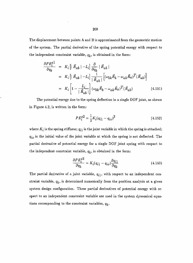
209

The displacement between points A and B is approximated from the geometric motion

of the system. The partial derivative of the spring potential energy with respect to

the independent constraint variable, is obtained in the form:

dPEf r ^ d --3^ =

Kb

= Ki 1 - ^ ^'^bk b '^ak (4.151) K b I J

The potential energy due to the spring deflection in a single DOF joint, as shown

in Figure 4.2, is written in the form;

- H o ) ^ (4.152)

where Ki is the spring stiffness; is the joint variable in which the spring is attached;

is the initial value of the joint variable at which the spring is not deflected. The

partial derivative of potential energy for a single DOF joint spring with respect to

the independent constraint variable, qf^, is obtained in the form:

(4.153)

The partial derivative of a joint variable, with respect to an independent con­

straint variable, q^, is determined numerically from the position analysis at a given

system design configuration. These partial derivatives of potential energy with re­

spect to an independent constraint variable are used in the system dynamical equa­

tions corresponding to the constraint variables, qf^.

Ci

Fi

Figure 4.2: Spring, damper and forces on a single DOF joint

211

Non-Conservative System Forces

The conservative forces are expressed in terms of the system potential energy

functions. The partial derivatives of the potential energy with respect to the indepen­

dent joint constraint and modal variables are used directly in the system equations

of motion. The contribution of generalized nonconservative forces and torques to the

system dynamical equations is determined by using the virtual work principle which

provides the compatible generalized nonconservative forces for Lagrange's approach.

For a force with magnitude Fj acting on body i along points A and B at point

C, as shown in Figure 4.3, the force vector is expressed in the form:

A = (4154) I ^ab I

where | | is the absolute magnitude of the vector R^i,- After substituting the

vector expression for the vector, Equation 4.154 is rewritten in the form:

Fi = - ••^oaFa) ,4,15g,

The virtual work corresponding to the virtual displacement of the independent con­

straint variable, is expressed in the form;

SW^ = E Fi • SRi = E {Fif { ^ \ % = (4-156) i=l i=l

fl where is the total number of applied forces; Qj^ is the generalized noncon­

servative force corresponding to the virtual displacement Sqf^ and is defined in the

form:

<?{' = ,E = gViFKkA} (4-157)

B

•1

C

Figure 4.3: Applied body force and torque

213

It is noted that the partial derivative of the general transformation matrix with

respect to an independent constraint variable, is known from the iterative position

analysis. No additional computations are required to determine the generalized force.

The vector for a torque applied on link i about a line passing through points

D and E, as shown in Figure 4.3, is represented in the form:

R de \^de (4.158)

The virtual work done by the torque due to virtual rotation of the body i is expressed

in the form:

90V swi, = E • «®i = E m) I a,,

2 = 1 i = l ! (4.159)

The rotational motion of link i is represented in by the 4x4 general transforma­

tion matrix. The partial derivative of the general transformation matrix with respect

to the independent constraint variable, imposes the effects of the variable, on

the translational and rotational motions of the link. The 4x4 matrix, [u'j/;,], repre­

sents both rotational and translational motions of link i with respect to the motion

of the variable, qj^, and may be written in the general form:

dOx

w i k \ =

0 dQ~

h

dQy

w 60; %

0

d Q x 0 % 0

0 0 0

dOy si

0

(4.160)

The upper-left hand corner of the matrix, represents the rotational derivative

of link i with respect to the variable, %. The partial rotational derivative, as used

214

in Equation 4.159, is obtained in the form:

m i -

dQx w;i(3.2)

0(yy < • = X

0 0

(4.161)

The virtual work due to applied torque corresponding to the virtual displacement,

8qf^, is determined by summing all the individual torques in the form:

N, tl •-1 = (4-162)

where N^-i is the total number of applied torques in the system; is the gen­

eralized nonconservative forces due to applied torques corresponding to the virtual

displacement 6% which is defined in the form:

(4.163)

The virtual work due to an applied force at a single DOF joint, as shown in Figure 4.2,

is written in the form:

N /2 N n 6W = ±' FiS,a = E

z = l i=l (4.164)

where #y2 is the total number of applied forces in the single DOF joints of the

f 2 . . system; is the generalized nonconservative force due to applied single DOF joint

forces corresponding to the virtual displacement, which is defined in the form:

iV,

(4.165) i=l

215

The virtual work due to an applied torque at a single DOF joint, as shown in Fig­

ure 4.2, is written in the form:

^t2 ^t2 a swk = Z nsqa = E Ti^stk = Qk^ik «-we)

i=l i=l

The generalized nonconservative force due to applied single DOF joint torques cor­

responding to the virtual displacement, 6qf^, is expressed in the form:

Nt2 o (4.167)

The generalized nonconservative force due to a damper connected to two different

bodies, as shown in Figure 4.1, is determined from the damping force as expressed in

the form:

Fi = -C'iiRcd • U^dWcd (4.168)

where Cj is the damping coefficient; is the unit position vector along the damper

centerline; is the relative velocity vector between points C and D and is obtained

in the form:

^cd = - -Rc = i'^da^d ~ ^ca-Rc)<?a (4.169) a=l

and the unit vector between points C and D is obtained in the form:

C'cd = "d - ' i c (4.170)

[ { R j - R c f i R i - i i c p

The virtual work due to the damping force corresponding to the virtual displacement,

6qf,, is expressed in the form:

• ^^cd

216

= - Q ( Kd • ^cd ) fh'dk & - '^ck M

-(4.171)

The generalized nonconservative force due to a two-point damper corresponding to

the virtual displacement, 6qj^, is defined in the form:

D F Qf = - - ca^c]^ c(/) % [^dk^d ' "^ckM 9% (4.172)

a=l

The virtual work due to a damper in a single DOF joint, as shown in Figure 4.2, is

obtained in the form:

&%1 6W}, = -C'iqiiôq^i = % (4.173)

The generalized force due to a single DOF joint damper corresponding to the virtual

displacement, 6qj^, is defined in the form:

Qa dqk ck=l

System Dynamical Equation for a Closed-Loop Mechanism

(4.174)

The system independent generalized variable vector is obtained by concatenating

the system independent joint constraint variables with the modal variables for all

the flexible links. With the expressions for the system kinetic and potential energy

functions and the generalized forces, the system equations of motion for closed-loop

mechanisms, as expressed in Equations 4.90, are obtained in the form:

[M) {%} + N

E U'=l

dM % {%}+U i k f

dM { % } = { Q c k + Q n k } (4.175)

217

The system inertia mass matrix, [M], is obtained from the system kinetic energy

functions, as expressed in Equation 4.125. The partial derivatives of inertia matrix

with respect to the independent joint constraint and modal variables are obtained

in Equations 4.126 through 4.133. The generalized conservative forces, are

determined from the partial derivatives of system potential energy functions due to

gravity, flexible deformations and idealized springs. The nonconservative forces due

to applied forces, torques and viscous dampers are determined from virtual work

principles.

218

CHAPTER 5. SUMMARY

The 4x4 transformation matrix methodology provides a unified approach for

the kinematic/dynamic analysis of open and closed-loop mechanisms. The kinematic

relationships are represented by the consecutive multiplications of the kinematic joint

transformation and link shape matrices.

Sheth and Uicker formulated the rigid link shape matrix relationships. This

concept is extended to handle flexible links in kinematic chains. The rigid link shape

matrix relates the translation position and angular orientation of one local joint

coordinate system relative to another system on the same link. The flexible link

shape matrix contains this same geometric data plus the elastic displacements and

rotations. Thus, the rigid link shape matrix becomes the special case of the flexible

link shape matrix. The small link elastic deformations of each link are approximated

by a limited number of mode shapes and modal displacements. The kinematic motion

of any point on a link is defined in terms of the joint constraint and modal variables.

An iterative position analysis is performed to determine the system DOF which

corresponds to the large displacement of the mechanism for each design configuration.

For open-loop mechanisms, the independent generalized coordinates include all the

joint constraint and selected modal variables. For closed-loop mechanisms, the inde­

pendent generalized coordinates include the independent joint constraint variables as

219

well as the selected modal variables. The system geometric matrix relates the motion

of the dependent joint constraint variables to the prescribed motion of the indepen­

dent joint constraint variables. The results from the iterative position analysis are

used to formulate the dynamical equations for geometrically-constrained, articulated

multi-link mechanisms.

The equations of motion for geometrically-constrained, articulated flexible and

rigid link mechanisms are formulated by Lagrange's approach. The number of dy­

namical equations is equal to the number of independent generalized coordinates that

are selected with the iterative position analysis procedure. The system kinetic and

potential energy functions were formulated in terms of the large displacement rigid

body motion (i.e., the joint constraint variables), and the small amplitude elastic

deformations. The potential energy function includes the effects due to gravity and

the elastic strain energy. The generalized conservative and nonconservative forces are

determined by the use of the virtual work principle.

220

BIBLIOGRAPHY

Wittenburg, J. 1977. Dynamics of systems of rigid bodies. Teubner, Stuttgart.

Paul, B. 1984. Computer-oriented analytical dynamics of machinery. Computer-Aided Analysis and Optimization of Mechanical Systems Dynamics, Series F: Computers and System Science 9:41-88. Springer-Verlag, Berlin.

Kane, T. R., and D. A. Levinson. 1985. Dynamics: Theory and applications. McGraw-Hill Book Co., New York.

Luh, J. Y. S., M. W. Walker, and R. P. C. Paul. 1980. On-line computa­tional scheme for mechanical manipulators. ASME J. Dyn. Sys. Meas. Control 102(2):69-76.

Hollerback, J. M. 1980. A recursive Lagrangian formulation of manipulator dynamics and a comparative study of dynamics formulation complexity. IEEE Trans. Syst. Man Cybern. SMC-10(ll):730-736.

Silver, W. M. 1982. On the equivalence of Lagrangian and Newton-Euler dy­namics for manipulations. Int. J. Robot. Res. l(2):60-70.

Featherstone, R. 1983. The calculation of robot dynamics using articulated-body inertias. Int. J. Robot. Res. 2(l):13-30.

Andrews, G. C., M. J. Richard, and R. J. Anderson. 1988. A general vector-network formulation for dynamic systems with kinematic constraints. Mecha­nism and Machine Theory 23(3):243-256.

Kane, T. R., and H. Faessler. 1984. Dynamics of robots and manipulators involving closed loops, pp. 97-106. in A. Morecki, G. Bianchi and K. Kedzior (eds.) Theory and Practice of Robots and Manipulators. Proc. of RoManSy'84: The Fifth CISM-IFToMM Symposium. Kogan Page, London.

221

10] Chace, M. A., and D. A. Smith. 1971. DAMN - Digital computer program for the dynamic analysis of generalized mechanical systems. SAE Paper 710244.

11] Orlandea, N., M. A. Chace, and D. A. Calahan. 1977. A sparsity - oriented approach to the dynamic analysis and design of mechanical systems: Part I and Part II. Trans. ASME J. Eng. Indust. 99:773-784.

12] Nielan, P. E. 1987. Efficient computer simulation of motions of multibody systems. Ph.D. Dissertation. Stanford University (Libr. Congr. Microfilms 8707714). Univ. Microfilms Int., Ann Arbor, Michigan.

13] Woo, L. S., and F. Freudenstein. 1971. Dynamic analysis of mechanisms using screw coordinates. Trans. ASME J. Eng. Indust. 93(l):273-276.

14] Yang, A. T. 1971. Inertia force analysis of spatial mechanisms. Trans. ASME J. Eng. Indust. 93(l):27-33.

15] Uicker, Jr. J. J. 1967. Dynamic force analysis of spatial linkages. ASME J. Appl. Mech. 34:418-424.

16] Uicker, Jr. J. J. 1969. Dynamic behavior of spatial linkages. Part I: Exact equations of motion. Part II: Small oscillations about equilibrium. Trans. ASME J. Eng. Indust. 91:251-265.

17] Sheth, P. N., and J. J. Uicker Jr. 1971. A generalized symbolic notation for mechanisms. Trans. ASME J. Eng. Indust. 93:102-112.

18] Sunada, W. H. 1981. Dynamic analysis of flexible spatial mechanisms and robotic manipulators. Ph.D. Dissertation. University of California, Los Angeles (Libr. Congr. Microfilms 8122862). Univ. Microfilms Int., Ann Arbor, Michigan.

19] Winfrey, R. C. 1971. Elastic link mechanism dynamics. Trans. ASME J. Eng. Indust. 93:268-272.

20] Winfrey, R. C. 1972. Dynamic analysis of elastic link mechanisms by reduction of coordinates. Trans. ASME J. Eng. Indust. 94:577-582.

21] Erdman, A. G., and G. N. Sandor. 1972. Kineto-elastodynamics - a review of the state of the art and trends. Mechanism and Machine Theory 7:19-33.

22] Erdman, A. G. 1985. Computer-aided design of mechanisms: 1984 and beyond. Mechanism and Machine Theory 20(4):245-249.

222

Neubauer, A. H., J. R. Cohem, and A. S. Hall. 1966. An analytical study of the dynamics of an elastic linkage. Trans. ASME J. Eng. Indust. 88:311-317.

Sadler, J. P., and G. N. Sandor. 1973. A lumped parameter approach to vi­bration and stress analysis of elastic linkages. Trans. ASME J. Eng. Indust. 95(2):549-557.

Alexander, R. M., and K. L. Lawrence. 1974. An experimental investigation of the dynamic response of an elastic mechanism. Trans. ASME J. Eng. Indust. 96:268-274.

Bahgat, B. M., and K. D. Willmert. 1976. Finite element vibrational analysis of planar mechanisms. Mechanism and Machine Theory 11:47-71.

Midha, A., A. G. Erdman, and D. A. Frohrib. 1978. Finite element approach to mathematical modeling of high-speed elastic linkages. Mechanism and Machine Theory 13:603-618.

Likins, P. W. 1972. Finite element appendage equations for hybrid coordinate dynamic analysis. Int. J. Solids Struct. 8:709-731.

Likins, P. W. 1973. Dynamic analysis of a system of hinge-connected rigid bodies with nonrigid appendages. Int. J. Solids Struct. 9:1473-1487.

Singh, R. P., and P. W. Likins. 1983. Manipulator interactive design with in­terconnected flexible elements, pp. 505-512. in Proceedings of 1983 American Control Conference, San Francisco, CA.

Singh, R. P., R. J. VanderVoort, and P. W. Likins. 1985. Dynamics of flexible bodies in tree topology - a computer-oriented approach. J. Guid. Control Dyn. 8(5):584-590.

Wielenga, T. J. 1984. Simplifications in the simulation of mechanisms contain­ing flexible members. Ph.D. Dissertation. The University of Michigan (Libr. Congr. Microfilms 8412279). Univ. Microfilms Int., Ann Arbor, Michigan.

BuflRnton, K. W. 1985. Dynamics of beams moving over supports. Ph.D. Disser­tation. Stanford University (Libr. Congr. Microfilms 8602460). Univ. Microfilms Int., Ann Arbor, Michigan.

Ryan, R. R., and T. R. Kane. 1985. Dynamics of a modula r space station. J. Astronautical Sci. 33(4):381-400.

223

[35] Ryan, R. R. 1986. Flexibility modeling methods in multibody dynamics. Ph.D. Dissertation. Stanford University (Libr. Congr. Microfilms 8612787). Univ. Mi­crofilms Int., Ann Arbor, Michigan.

[36] Judd, R. P., and D. R. Falkenburg. 1983. Dynamics of nonrigid articulated robot linkages, pp. 1045-1049. in Proceedings of 1983 American Control Conference, San Francisco, CA.

[37] Book, W. J. 1984. Recursive Lagrangian dynamics of flexible manipulator arms. Int. J. Robot. Res. 3(3):87-101.

[38] Song, J. 0., and E. J. Haug. 1980. Dynamic analysis of planar flexible mecha­nisms. Comp. Meth. Appl. Mech. Eng. 24:359-381.

[39] Guyan, R. J. 1965. Reduction of stiffness and mass matrices. AIAA Journal 3(2):380.

[40] Irons, B. 1965. Structural eigenvalue problems: elimination of unwanted vari­ables. AIAA Journal 3:961-962.

[41] Hurty, W. C. 1965. Dynamic analysis of structural systems using component modes. AIAA Journal 3:678-685.

[42] Morris, N. P. 1977. The use of modal superposition in nonlinear dynamics. Comp. and Struct. 7:65-72.

[43] Nickell, R. E. 1976. Nonlinear dynamics by mode superposition. Comp. Meth. Appl. Mech. Eng. 7:107-129.

[44] Maddox, N. R. 1975. On the number of modes necessary for accurate response and resulting forces in dynamic analysis. ASME J. Appl. Mech. 42:516-517.

[45] Turcic. D. A. 1982. A general approach to the dynamic analysis of elastic mech­anism systems. Unpublished Ph.D. Dissertation. The Pennsylvania State Uni­versity, University Park, Pennsylvania.

[46] Turcic, D. A., and A. Midha. 1984. Dynamic analysis of elastic mechanism systems. Part I: Application. ASME J. Dyn. Sys. Meas. Control 106:249-254.

[47] Turcic, D. A., A. Midha, and J. R. Bosnik. 1984. Dynamic analysis of elastic mechanism systems. Part II: Experimental results. ASME J. Dyn. Sys. Meas. Control 106:255-260.

224

Shabana, A. A. 1982. Dynamic analysis of large scale inertia-variant flexible systems. Ph.D. Dissertation. The University of Iowa (Libr. Congr. Microfilms 8310084). Univ. Microfilms Int., Ann Arbor, Michigan.

Shabana, A. A. 1985. Automated analysis of constrained systems of rigid and flexible bodies. ASME J. Vib. Acous. Stress Reliab. Des. 107:431-439.

Shabana, A. A. 1986. Dynamics of inertia-variant flexible systems using exper­imentally identified parameters. ASME J. Mech. Trans. Autom. Des. 108:358-366.

Shabana, A. A. 1986. Transient analysis of flexible multi-body systems. Part I: Dynamics of flexible bodies. Comp. Meth. Appl. Mech. Eng. 54:75-91.

Shabana, A. A., R. D. Patel, A. DebChaudhury, and R. Ilankamban. 1987. Vi­bration control of flexible multibody aircraft during touchdown impacts. ASME J. Mech. Trans. Autom. Des. 109:270-276.

Shabana, A. A., and B. Thomas. 1987. Chatter vibration of flexible multibody machine tool mechanisms. Mechanism and Machine Theory 20(4):359-369.

Agrawal, 0. P. 1984. Application of deformable body mean-axis to dynam­ics of flexible mechanical systems. Ph.D. Dissertation. University of Illinois at Chicago (Libr. Congr. Microfilms 8501232). Univ. Microfilms Int., Ann Arbor, Michigan.

Agrawal, 0. P., and A. A. Shabana. 1986. Automated visco-elastic analysis of large scale inertia-variant spatial vehicles. Comp. and Struct. 22(2):165-178.

Agrawal, 0. P., and A. A. Shabana. 1986. Application of deformable-body mean axis to flexible multibody system dynamics. Comp. Meth. Appl. Mech. Eng. 56:217-245.

Wehage, R. A., and E. J. Haug. 1982. Generalized coordinate partitioning for dimension reduction in analysis of constrained dynamic systems. Trans. ASME J. Mech. Des. 104:247-255.

Singh, R. P., and P. W. Likins. 1985. Singular value decomposition for con­strained dynamical systems. ASME J. Appl. Mech. 52:943-948.

Mani, N. K., and E. J. Haug. 1985. Singular value decomposition for dynamic system design sensitivity analysis. Engineering with Computers 1:103-109.

225

[60] Liang, C. G., and G. M. Lance. 1987. A difFerentiable null space method for constrained dynamic analysis. ASME J. Mech. Trans. Autom. Des. 109:405-411.

[61] Wampler, C., K. Buffinton, and J. Shu-hui. 1985. Formulation of equations of motion for systems subject to constraints, ASME J. Appl. Mech. 52:465-470.

[62] Wang, J. T., and R, L. Huston. 1987. Kane's equations with undetermined multipliers-application to constrained multibody systems. ASME J. Appl. Mech. 54:424-429.

[63] Amirouche, F. M. L., and T. Jia. 1987. Automatic elimination of the undeter­mined multipliers in Kane's equations using a pseudo uptriangular decomposi­tion (PUTD) method. Comp. and Struct. 27(2):203-210.

[64] Amirouche, F. M. L., and T. Jia. 1988. Pseudouptriangular decomposition method for constrained multibody systems using Kane's equations. J. Guid. Control Dyn. ll(l):39-46.

[65] Chang, C. 0., and P. E. Nikravesh. 1985. An adaptive constraint violation stabilization method for dynamic analysis of mechanical systems. ASME J. Mech. Trans. Autom. Des. 107:488-498.

[66] Chang, C. W., and A. A. Shabana. 1987. Hybrid control of flexible multi-body systems. Comp. and Struct. 25(6):831-844.

[67] Sheth, P. 1972. A digital computer based simulation procedure for multiple de­gree of freedom mechanical systems with geometric constraints. Ph.D. Disser­tation. The University of Wisconsin-Madison (Libr. Congr. Microfilms 732565). Univ. Microfilms Int., Ann Arbor, Michigan.

[68] Sheth, P. N., and J. J. Uicker Jr. 1972. IMP (integrated mechanisms program), a computer-aided design analysis system for mechanisms and linkage. Trans. ASME J. Eng. Indust. 94:454-464.

[69] JML Research, Inc. 1988. The integrated mechanisms program (IMP): Lan­guage specification and user's manual. JML Research, Inc., Madison, Wiscon­sin.

226

PART III.

SIMULATION ALGORITHMS AND DEMONSTRATION EXAMPLES

227

CHAPTER 1. INTRODUCTION

The equations of motion for multi-link, geometrically-constrained rigid/flexible

mechanical systems represent the relationship of system geometric constraint and

elastic modal variables with respect to the system inertia properties and external

applied forces. The procedure of formulating these equations provides a theoretical

background for developing general-purpose simulation programs. Tremendous effort

and research have been conducted to develop general-purpose, user-friendly programs

as shown in Part I. This research provided an additional feature for the existing

computer simulation programs where mechanical systems were modelled as rigid-

body assemblies.

The algorithm was developed to handle general mechanical systems: either open

or closed-loop mechanisms. For open-loop mechanical systems, the motion of every

joint variable needs to be determined either from external applied forces or from

specified motion input. For closed-mechanical systems, the additional geometric con­

straints reduce the total degrees of freedom, the motion of the system is then deter­

mined by considering both geometric constraint equations and dynamic equations.

The simulation algorithms were developed for both types of mechanical systems.

Chapter 2 presents the procedures for determining the system equations of motion in

a systematic approach. The capability of the existing rigid-body simulation programs

228

could be enhanced once the algorithm is incorporated into the program, which is the

logical step for further research.

The basic modelling concepts and the simulation procedures were demonstrated

in the third chapter of this part. Three simplified examples were discussed: (1) a

double pendulum problem which represented an open-loop mechanical system; (2)

a mobile crane problem which was modelled as an extended open-loop mechanical

system; and (3) a front-end loader which was modelled as the closed-loop mechanical

system.

The first example was used to demonstrate the basic modelling concepts: def­

inition of local coordinate systems, determination of geometric constraint matrices

for pin joints and definition of flexible link shape matrix. The kinematics of the

system was studied for both rigid and flexible links. The equations of motion for

a rigid body system were obtained in an exact form. Mode shape functions were

used to estimate the elastic deflection of the links. The complexity of introducing

the flexibility into the modelling process was observed when the equations of motion

for the flexible systems were formulated in the same fashion. The rigid body model

represented the large-displacement motion of the system with the flexibility being

ignored. The equations of motion for the flexible system were formulated by intro­

ducing additional modal variables. A case study was conducted for a selected set of

parameters using a numerical integration technique. The efl^ects of link flexibility on

the system performance were observed.

The mobile crane was modelled as an extension of the double pendulum problem

by considering the vertical, pitch and roll motion of the chassis. The lifting boom was

modelled as an extendable collection of beams with end support. The orientation and

229

length of the boom were controlled by the operator during the operation process. The

equations of motion for the system were formulated using the 4x4 matrix approach.

The motion animation was conducted to study the rigid-body motion pattern and

the configuration of the system. The transient dynamic response of the system was

studied by numerically integrating the system equations of motion from estimated

system parameters and initial values.

The front-end loader was modelled as a moveable chassis with closed-loop linkage

attached to it. The large displacement motion of the entire system was modelled for

the working process. The lifting motion of bucket was controlled by the motion of the

lifting cylinder. The kinematics of the linkage system with respect to the chassis was

studied to demonstrate the geometric constraints for a closed-loop mechanical system.

The elastic deflection of the linkage due to external load was studied using finite

element method with the chassis being treated as an external constant boundary.

Three simplified examples were used to demonstrate the basic modelling pro­

cedure. The in-depth study of a general mechanical system composed of both rigid

and flexible members could be conducted when a general program is developed by

incorporating this algorithm. The simplified examples also serve as the validation for

the simulation program.

230

CHAPTER 2. SIMULATION ALGORITHM DEVELOPMENT

The system equations of motion have been developed corresponding to the joint

and modal displacements. The implementation of Equations 3.86 and 3.87 of Part

II into a simulation program needs to be further discussed because the equations

include the second derivatives of the transformation matrices which are complex

functions of the joint and modal displacements as well as the time derivatives of

those independent variables. The unknown second order derivatives and their inertia

coefficients are placed on the left hand side of the equation while all force effects are

on the right hand side of the equation and the system equation is expressed in the

general form:

where M is the equivalent mass matrix which represents the inertial properties of the

system; {q} is the generalized independent variables which are defined in the form:

The equivalent force vector {F}, which includes all external force inputs, the damping

and the stiffness effects, are defined corresponding to the generalized independent

Algorithm for Open-Loop Mechanical Systems

|M| {,} = {F} (2 .1)

19111912' "•'^ITV^ ' 12' ^Imj^ ' •

'?nl'9n2' "•'9njV7i'^nl'^n2' •••iVnmn^ (2.2)

231

variables;

{ ^ } — | / l l ) / l 2 ' • • • ' / l ' / i l ' / l 2 '

/n i ' /n2' '" ' /n iVra' '" ' /n i ' /TO2' • • •^fnmn} (2-3)

where fj^ is the force function corresponding to the joint variable qj^; fj^ is the force

function corresponding to the elastic body modal variable rjja- The dynamic behavior

of the system is evaluated by solving Equation 2.1 with given initial conditions.

Inertia coefficients of the system dynamic equation

The inertia coefficients that multiply the second derivatives of the joint and

modal displacements with respect to time are determined from Equations 3.86 and

3.87 of Part II, respectively. The partial derivatives of the general transformation

matrix with respect to the joint and modal displacements are expressed in the forms;

d A ' -dqj^ ~ — ^ ^ (2.4)

^ ; + 1 < ! < n (2.5)

The second derivatives of the general transformation matrix with respect to time are

determined from Equation 3.23 of Part II.

Inertia coefficients from the joint equation The second-order time deriva­

tive of the joint displacement (i.e., qj^) appears only in the second-order time deriva­

tive of the general transformation matrix (i.e., A^j). The inertia coefficient for

from the equation corresponding to the joint constraint variable, qj^,, is determined

232

by considering the first portion of Equation 3.86 of Part II and is expressed in the

form:

n

n =

i = j

d A

^ 4 4 ^9ja.

— E Z ^o,h-lQhl3^h-l,ihf3 +-y;i=l^=l

(2 .6)

It is noted that the joint displacement qj^ influences the motion of all the bodies

from body j to body n in the system. The second derivative of the joint displacement,

influences the motion from body h to body n in the system. The coefficient for

from the equation corresponding to the joint constraint variable, must be

determined by considering all the bodies influenced by joint j and a successive joint

h simultaneously. The summation operation on all possible bodies to be considered

in this process is rewritten in the form:

n n E. E = E E i = j h — l h = l i = m a x { j , h )

(2 .7)

The inertia coefficient of with respect to the joint variable, qj^,, is obtained in

the form:

~ '^o,j — lQja^^jhQhl3'^o,h-l

J — 1,2,...,71^ Û! — 1,2,..., iVj

h = l,2,...,n; ( 3 = 1,2,...,A''^ (2.8)

where is the inertia property of all bodies due to the effects of joint variables,

qj(^ and and is defined in the form:

i = m a x { j , h ) (2 .9)

233

Based on the matrix trace operation property, the switch of the subscripts of the

inertia coefficient does not change its value (i.e., means

that the inertia coefficient for with respect to qj^ has the same value as the

inertia coefficient for with respect to This symmetry property is used to

reduce the computation.

The computation of the inertia coefficient for the second-order time derivative

of the modal displacement (i.e., with respect to qj^^ varies depending upon

the relative location of the flexible body h and the joint j in the system. When the

flexible body h is beyond the joint j (i.e., h > j), is computed by considering

all the bodies from body h to body n in the system. When the flexible body h is

before the joint j relative to the global inertial frame, the inertia coefficient Mj^

is determined by considering all the bodies from the body j to body n in the system.

When body n in the system is considered, the inertia coefficient for with

respect to qj^ is determined by considering body n only. The second-order time

derivative of the general transformation matrix Aon does not include the modal

accelerations of body n (i.e., Only the third term on the left hand side of

Equation 3.86 in Part II involves The inertia coefficient for j corresponding

to all the joint variables qj^ is expressed in the form:

^^ja,nf3 ~ — ja-^j—l,n^nl3^on\

j = 1,2, . . . , 7 i ; a = 1 , 2 , l 3 = 1 , 2 , . . . , m n (2.10)

When the flexible body h is beyond the joint j (i.e., h > j ) , all the bodies from body

h to body n in the system are influenced by The inertia coefficient for with

234

respect to jth joint is expressed in the form:

M j a , h f 3 = T r

j = l ,2 , . . . ,n , - 1; h = j , j + 1 , . . . ,n - 1 (2.11)

where is the inertia property of all bodies due to the joint variable, qj^^, and

modal variable, and is defined in the form:

= n

E i = m a x { h + l , j )

(2.12)

When the location of flexible body h is closer to the fixed coordinate system origin

than that of the joint j (i.e., h < j), all the bodies from body j to the end of the

system are influenced by both the joint variable, and the modal variable, Vhf3-

^^ja,hf3 then expressed in the form:

'"^oJ-lQja h hlS'^oh

J — 2,3,...,72-5 h — l,2,...,j 1 (2.13)

The inertia coefficients for qj^^ and from the equation of motion correspond­

ing to the joint variable, qja^ are completely determined.

Inertia coefficients from the modal variable equation The inertia co­

e f ficient for qj^ from Equation 3.87 of Part II corresponding to [h > j) is

determined by considering all the bodies from body h to body n in the system and

is expressed in the form:

^^hl3,ja =

j = l ,2 , . . . ,n- l ; h = j , j - f 1 , . . . ,n - 1 (2.14)

235

It is noted that the coefficient for with respect to qj^, as shown in Equation 2.11,

is the same as the coefficient for with respect to 7;^^, as shown in Equation 2.14.

This symmetry property between the joint and the modal variables is used to reduce

the computation during the simulation.

The inertia coefficient for the last body modal acceleration with respect to

the Tjna is determined by considering body n in the system and is expressed in the

form:

(2.15) ^na,nl3 4 f'T aT

The matrix trace operation has the same value when the matrices change the order

under cyclic permutation and is shown in the form:

T r [ A B C ] = T r [ B C A ] = T r [ C A B ] (2.16)

The matrix C^^^ has zeros in its last column and row because the product of the

transformation matrix A^yiAon has a 3 x 3 identity submatrix in the upper left corner.

The trace operation on the inertia coefficient is expressed in simplified form:

^*'^na,ni3 ~ (2-lT)

For the diagonal terms (i.e., j = h = l,2,...,n — 1), the inertia coefficient for 7/^^

with respect to is determined by considering all the bodies from body h to body

n in the system and is expressed in the form:

^^ja,hl3 ~ hex(3

j = h = 1 ,2 , . . . , n - 1 (2 .18 )

where is the inertia property of all bodies under the effects of modal variables,

236

t/ j q, and 7/^^, and is expressed in the form:

n Wjh = E

i — m a x { h + l , j + l ) (2.19)

The inertia coefficient for the modal acceleration of body n (i.e., from the

previous modal variable equations (i.e., l<j = /i<n — l)is determined by

considering the motion of the last body influenced by the modal variable rjj^ and is

expressed in the form:

^^ja,nl3 [-^oj^ja'^jn^n/3'^ori\

J — 1 ,2 , . . . , 72 I j ft — Tt (2.20)

The inertia coefficient for the modal acceleration 7^^ with respect to j ]j^ with h

greater than j is determined by considering all the bodies from body h to body n in

the system and is expressed in the form:

j = l ,2 , . . . ,n- l ; h = j + l , j + 2 , . . . , n - 1 (2.21)

The inertia coefficient for modal acceleration iij^ with respect to 77^^ with j less

than h is determined by considering all the bodies from body h to body n of the

system and is expressed in the form:

^^h(3,ja = ^oh^h(3^^jh^ja^oj ^oj^ja-^jh^hf3-^oh

1,2,...,71 — 1; h — _y + l, j + 2, . . . , 77 — 1 (2.22)

It is has been shown that the inertia coefficient for 17^^ with respect to is the

same as the coefficient for with respect to This symmetry property between

237

the modal variables is used to reduce the computation of inertia coefficients during

the simulation.

The computation of all inertia coefficients for the second-order time derivatives of

joint and modal variables are completely determined by using the symmetry property

among the independent variables. The unknown second-order time derivatives of the

variables can be determined by pre-multiplying the inverse of the inertial matrix with

the generalized force vector.

Generalized force vector

The equivalent forces corresponding to the generalized independent joint and

modal displacements are determined from Equations 3.86 and 3.87 of Part II.

The generalized force corresponding to the last joint variable in the system, qna-,

is determined from Equation 3.86 of Part II and is expressed in the form:

It is noted that the force includes three parts: (1) the Coriolis acceleration effects; (2)

the gravity effects, and (3) the generalized applied forces. The Coriolis acceleration

effects are defined in simplified form:

(2.23)

(2.24)

The gravity effect is defined in simplified form:

mn Pn =Bn+ E

13=1 (2.25)

238

Substituting Equations 2.24 and 2.25 and the partial derivatives of the general trans­

formation matrix with respect to the generalized joint variable, qj^, the equivalent

force for the last joint variable is expressed in the form:

fna = Tr [ ^ o , n — — - ^ n ) ] + Fna (2.26)

For an open-loop mechanical system, the force is transferred from one body to

the next one through the joint transformation matrices. For a given body j, the

Coriolis acceleration effect is computed by the backwards recursive formula:

rrij

~ ^ S j/3^jj3-^oj ^j,j+l^j+l^j+l (2.27) f3=l

The gravity effect for a given body j is also computed recursively backwards along

the chain in the form:

Pj = + E VjisGjiS + (2.28) (3=1

After defining those recursive formulae, the equivalent force corresponding to a given

joint variable is computed recursively backwards along the chain in the form:

f j a = [ ' ^ o , j - l Q j a ^ j - l , j { P j ~ j ) ] + j a

j = l , 2 , . . . , 7 i ; a = 1 , 2 , . . . , Nj (2.29)

The Coriolis acceleration effects and the gravity effects for body n are computed

by using Equations 2.24 and 2.25, respectively. The rest of the terms are computed

recursively backwards using Equations 2.27 and 2.28. The equivalent force corre­

sponding to joint n's displacement as defined in Equation 2.26 is computed first.

The equivalent force corresponding to the rest of the joint variables is computed

recursively backwards using Equation 2.29.

239

The generalized force corresponding to body n's modal displacement r]na is

determined from Equation 3.87 of Part II and is expressed in the form:

/; nl3 = Tr

mn ^onG^jj - \^rnD^i^ + 2Âon ^ j Aq^

mn

- I] VnaKji^a a = l

(2.30)

It is noted that the equivalent force for the modal displacement also includes three

parts: (1) the gravity effect, (2) the Coriolis acceleration effects, (3) the elastic deflec­

tion effects. The generalized applied forces are assumed to be applied in such a way

that only the joint displacements are directly influenced because the elastic defor­

mation is small in comparison with the motion of large- dis placement joint variables.

Using the definitions for Coriolis acceleration effects and the gravity effects in Equa­

tions 2.27 and 2.28, the equivalent force corresponding to the modal displacement

r]j^ is computed recursively backwards and is expressed in the form:

~ {^j+1 ~ j+l)

/ mj

oj ^ ja^' .T

o j ^ • i j a j f 3 a a = l

A OJ

mj

S ja^jl3a Q = 1

J — l , 2 , . , . , 7 t jS — 1,2,. . . , 7 7 2 » (2.31)

The force vector corresponding to the joint and modal displacements is com­

pletely determined. The simulation algorithm provides a systematic approach of

adding flexibility features into open-loop, existing rigid-body simulation programs.

240

Algorithm for Closed-Loop Mechanical Systems

The dynamic response of a geometrically-constrained mechanical system may be

determined by solving the second-order differential equations and the system geo­

metric constraint algebraic equations at any given system configuration. The natural

frequencies and damping coefficients, which are functions of the system configura­

tion, may be obtained from the linearized system dynamic equations about a given

static equilibrium configuration. The solution of the linearized dynamical equations

requires much less computational effort than that for nonlinear equations. The mode

superposition technique may be used to evaluate the system responses for different

external force excitations.

To linearize the dynamical equations for a generalized geometrically-constrained

mechanical system, the static equilibrium position must be determined by considering

the constant terms of the externally applied forces and the specified joint constraint

variable motions. The generalized time dependent variables which include both the

joint constraint and modal variables about the static equilibrium position may be

written in the from:

where is the N x I vector containing the generalized constraint variables

and modal variables; is the jV x 1 vector containing the known values at the

static equilibrium position of the system; is the A'" x 1 vector containing the

variational variables determined at the static equilibrium position. The perturbation

velocities and accelerations of the system variables are expressed in the form:

{%(^)} = {%}* + (2.32)

{%(0} = {4(0} (2.33)

241

and

{%(')} = ÂW) (2-34)

The specified constraint motions in each of the vectors {5}, {5}, and {6} are assumed

to be known. After substituting the perturbation variables, Equation 4.175 of Part

II is written in the form:

[M]{h} + dM • N

[S "'J (4) = {Qnk + Qck} - {4}^

d[M]

. ^1k . {4} (2.35)

The mass [M] and damping [C\ matrices may be approximated by a Taylor series

expansions about those known matrices at the static equilibrium position:

N [M] = [M], + E

i=l

1 N N

and:

i= l i= l

N [C| = |C'|.+ E

i= i

, N N 4- S

i=lj=l

dM

. 9qi J

d'^M

dqidqj

ac

+ (2.36)

^9% J

d'^C

dqidqj Si6j + (2.37)

The nonconservative forces may be expressed in the form:

= (ft). + {PkW} - ICI. {4} (2.38)

where is the generalized forces resulting from the constant terms of the external

applied forces; {Pf^(t)} is the generalized forces resulting from the variable terms of

the external applied forces. The last term in the equation is the contribution of

damping effects to the system generalized forces.

242

The conservative forces may be expanded using the Taylor series at the

static equilibrium position:

From the system potential energy definition, it is known that the system conservative

forces are determined from the partial derivative operations of the potential energy

function:

Thus, Equation 2.39 is rewritten in terms of the system potential energy functions:

Because the variational motion about the static equilibrium position is small,

the second and all higher order terms in the equation may be neglected. Substituting

the Taylor expansions for the system mass, stiffness and damping matrices, as well

as the conservative and nonconservative forces into the system dynamical equation.

Equation 4.175 of Part II may be written in the form:

I M ] , { « } = { P k h + { P k W } - |C|. {i} + ( Q c k h - m» CI} (2-42)

At the static equilibrium position, the constant part of externally applied forces is

equal to the constant part of the system conservative forces:

(2 .39)

(2.40)

{Pk}* + {Qck}* = 0 (2.43)

243

Thus, the linearized system dynamic equations of motion may be expressed in a

standard form:

|M|. {«} + PI. {<} + [A'l, {«} = {?(,(()} (2.44)

The coefficient matrices [M], [C], and [if] are well-defined quantities determined at

the static equilibrium position.

244

CHAPTER 3. DEMONSTRATION EXAMPLES

Example 1: Double Pendulum Problem

A double pendulum as shown in Figure 3.1 has two links with lengths Li and L2,

respectively. The first link rotates about a fixed pin joint (JNTl), the other end of the

link is connected to the second link through a pin joint (JNT2). Two joint variables

{9i and O'j) are used to represent the rotational position of the large-displacement

rigid-body system. The first variable ) represents the absolute rotational motion of

link one, while the second variable (^2) represents the relative rotation of the second

link with respect to the first one. The mass of the link is modelled as a point mass

at the end of the link {mi and mg) and distributed mass along the link is ignored

[1-6].

The first joint (JNTl) allows the rotational motion of the first link about a fixed

axis and is modelled by considering the relationship between the two coordinate

systems: XYZ and where the coordinate system XYZ is fixed in space

and the coordinate system x-^y-^zi is fixed on the lower end of the first link. The

relationship between the two coordinate systems is represented by the first joint

245

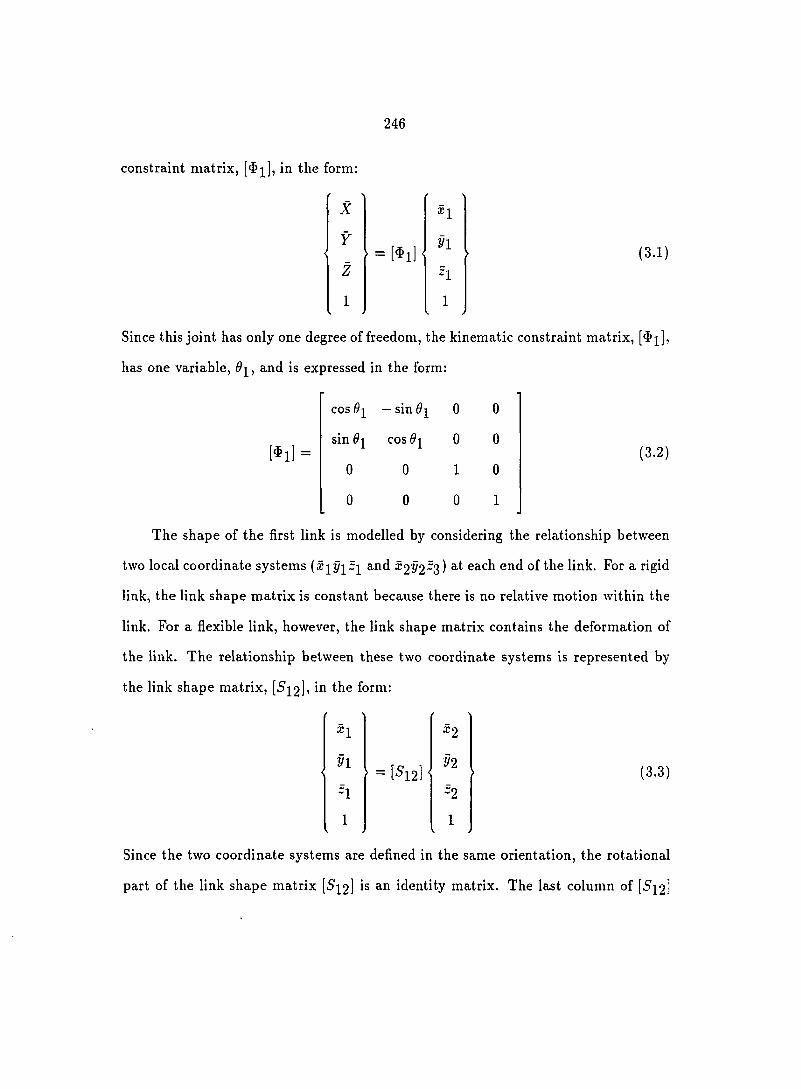
246

constraint matrix, [$]^], in the form:

X XI

Y , = [#2! ' h

Z h

1 1

(3 .1)

Since this joint has only one degree of freedom, the kinematic constraint matrix, [$i],

has one variable, ^2, and is expressed in the form:

[ $ l ] =

cos — sin 0 0

sin cos 0 0

0 0 1 0

0 0 0 1

(3.2)

The shape of the first link is modelled by considering the relationship between

two local coordinate systems and X22/2^3) sach end of the link. For a rigid

link, the link shape matrix is constant because there is no relative motion within the

link. For a flexible link, however, the link shape matrix contains the deformation of

the link. The relationship between these two coordinate systems is represented by

the link shape matrix, in the form:

'

XI ^2

yl . = [5i2] < n

h ~2

1 1

(3.3)

Since the two coordinate systems are defined in the same orientation, the rotational

part of the link shape matrix is an identity matrix. The last column of [6'%2i

247

represents the location of the origin of the coordinate system ®2^2^2 ^ith respect

to the coordinate system The link shape matrix for the first link is then

expressed in the form:

[•^12]

1

0

0

0

0 0

1 0

0 1

0 0

h

0

0

1

(3.4)

With the same procedure, the second joint is modelled by considering the relative

motion of the coordinate system 53^323 with respect to the coordinate system ^2%^2

and is expressed in the form:

'

^2 ^3

h < ' = [^2] ' h

-2 -3

1 1

(3.5)

the elements in the second joint constraint matrix, [$]2) are defined in the form:

[^2] =

cos 2 — sin ^2 0 0

sin 2 cos 2 0 0

0 0 1 0

0 0 0 1

(3.6)

The location of the point mass and m^) is represented by the local posi­

tion vector in the local coordinate systems and ^3^323, respectively, and is

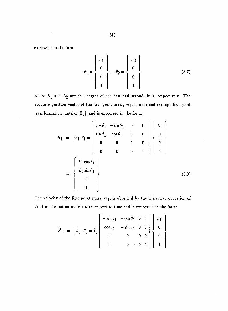
248

expressed in the form:

ri = <

L l L 2

0 0 > ; f2 = <

0 0

1 1

(3.7)

where Li and L2 are the lengths of the first and second links, respectively. The

absolute position vector of the first point mass, is obtained through first joint

transformation matrix, [#i], and is expressed in the form:

^1 = =

Li cos

Li sin

0

1

cos 61 - sin 2 0 0 Ll

sin $1 cos 0 0 0 sin $1 <

0 0 1 0 0

0 0 0 1 1

(3.8)

The velocity of the first point mass, mj, is obtained by the derivative operation of

the transformation matrix with respect to time and is expressed in the form:

^1 = [^1] 1 =

— sin — cos 9^ 0 0 Ll

cos — sin 0 0 0

0 0 0 0 0

0 0 • 0 0 1

249

—^2^2 sin

Liè- cos 9-

0

0

(3.9)

The absolute position vector for the second point mass, mg, on the tip of the

second link is obtained through the multiplication of the consecutive transformation

matrices of joint one, link one and joint two, and is expressed in the form:

^2 = [^l][-^12][^2]^

cos 9-^

sin 9i

0

0

cos ^2

sin ^2

0

0

- sin 9^

cos 9-

0

0

— sin ^2

cos ^2

0

0

0

0

1

0

0

0

0

1

0

0

1

0

0

0

0

1

1

0

0

0

L'l

0

0

1

0

1

0

0

h

0

0

1

^2 cos(^2 + ^2) ^1

f 2 sin(^2 + ^2) + sin 9 ^

0

1

(3 .10 )

For a rigid body system, the link shape matrix and the local position vector

are constant and their derivatives with respect to time are zeros. The velocity of

the point mass, 7772, is obtained by differentiating the transformation matrices and

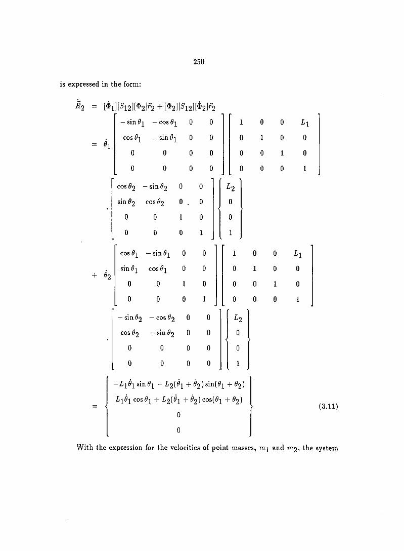
250

is expressed in the form:

4

= 9

[^I][*5'I2][^2F2 + [^2l['^12][^2]^2

- sin 2 — cos ^2 0 0

cos 0-^ — sin 0 0

0 0 0 0

0 0 0 0

1

0

0

0

cos ^2 — sin ^2 0 0 ^2

sin 2 cos $2 0 . 0 0

0 0 1 0 0

0 0 0 1 1

+ ^2

0

0

1

0

L l

0

0

1

COS 9 i — sin 0 0 1 0 0 Ll

sin COS 0 0 0 1 0 0

0 0 1 0 0 0 1 0

0 0 0 1 0 0 0 1

— sin 62 — cos ^2 0 0 I2

COS O2 — sin ^2 0 0 0

0 0 0 0 0

0 0 0 0 1

(3.11)

— sin^]^ - 2(^1 + 2)sin(^2 + O 2 )

L^O-j^ cos9-^ + ^2(^1 + ^2) cos(0]^ + 2)

0

0

With the expression for the velocities of point masses, and m2, the system

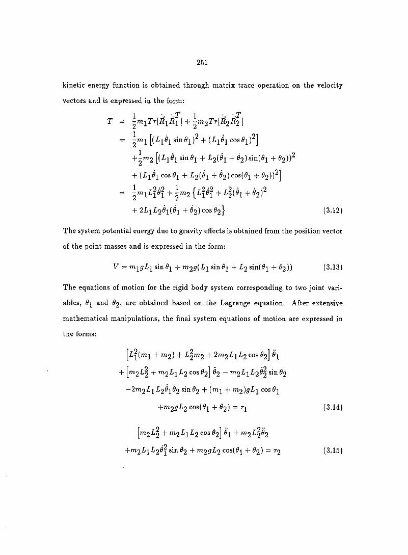
251

kinetic energy function is obtained through matrix trace operation on the velocity

vectors and is expressed in the form;

T = ^ m i T r [ R i R i ] + m 2 T r [ R 2 R 2 ]

= sin^]^)^ + { L i è i cos0]^)^j

+ 2^2 [(-^1^1 sin0]^ + L 2 ( è i + 02)sin(0]^ + 2))^

+ (^1^1 cos $1 + 12(^1 + 2) + 2))^]

+ 2i^^f 2^1(^1 + 2) ^2} (3.12)

The system potential energy due to gravity effects is obtained from the position vector

of the point masses and is expressed in the form:

V = m i g L i s i n + m 2 g ( L i sin + L 2 sin(^2 + ^2)) (3.13)

The equations of motion for the rigid body system corresponding to two joint vari­

ables, 6^ and $2^ are obtained based on the Lagrange equation. After extensive

mathematical manipulations, the final system equations of motion are expressed in

the forms:

-f 7712) + •t2"^2 + 277122)1^2 cos 2]

+ 212 + "T^2^1^2 cos 2] ^2 — "T^2^1^2^2 ®^^^2

—27772X]^ 12^1^2 sill 2 + (^1 + ^712)^^1 cos0]^

+7772^^2 cos(^2 + ^2) " n (3.14)

1^7772^2 cos ^2] + 2^2*^2

-{-7772£i£2^1 sin ^2 + 23^2 cos(0j^ 4- $2) — "^2 (3.15)

252

where and rg are applied torques at joints one and two, respectively.

The effects of link flexibility on the system dynamic behavior are explored by

considering the flexibility of the links in formulating the system equations of motion.

The first mode of vibration for each link is used in the formulation. Two additional

variables, and «2, are introduced to represent the flexible system configuration as

shown in Figure 3.2.

For this simplified problem, the fixed-free mode is used to represent the vibra­

tional motion of the link. The rotational angle, 7, at the end of the link is related to

the deflection at the same location of the link in the form:

3ui (3.16)

The deformation of the link changes the location and orientation of the local coor­

dinate system (52^2-2) ^^ith respect to the local coordinate system (.-ciyicj) at the

lower end of the link. Thus, the link shape matrix is modified to reflect the shape

change of the flexible link. For small elastic deformation, the rotational angle is

small and the assumption, sin 7 =2 7 and cos 7 % 1, is often used. The deformation

matrix in this example uses the exact notation to simplify the hand calculation of

mathematical manipulations in deriving system equations of motion. The link shape

matrix for the first link, [5i2]) is modified in the form:

.•Cl 1 0 0 II

h 0 10 0 <

:1 0 0 10

1 0 0 0 1

cos 7 - sin 7 0 0 ^2

sin 7 cos 7 0 "1 <

n

0 0 1 0 -2

0 0 0 1 1

Ql Ll

Figure 3.2: Double pendulum (flexible body system)

COS 7 —sin 7

sin 7 cos 7

0 0

0 0

254

h

H

0

1

^2 X 2

. n

. = [5i2] • n

:2 ^2

1 1

(3.17)

The local position vectors for the point masses, mi and m2, are modified by including

the transverse deformation terms, uj and U2, and are expressed in the forms;

r i =

h h

H «2 . ; f2 = <

0 0

1 1

(3.18)

The global position vector of the point mass, m is obtained through transfor­

mation matrix operation as expressed in the form:

R l =

cos 6i - sin 0 0 Ll

sin 9i cos 01 0 0 «1 <

«1 1 — <

0 0 1 0 0

0 0 0 1 1

Li cos $1 — sin

Li sin 61 + cos Oi

0

1

.(3.19)

For flexible links, the derivative of local position vector with respect to time is no

longer zero due to vibrational motion. The velocity of the point mass, mi, contains

velocities of both large rotational motion of the first joint and the small vibrational

motion of the link and is expressed in the form:

^1 = [^lln +

255

= h

— sin^]^ — cos Oi 0 0 L l

cos — sin 9^ 0 0 <

"1

0 0 0 0 0

0 0 0 0 1

+

COS 9- — sin 61 0 0 0

sin cos 9^ 0 0 «1 sin cos 9^ 4

0 0 1 0 0

0 0 0 1 0

— sin^^ — cos0]^ — sin^]^

L-^Oi cos — uièi sin + tq cos^^

0

0

(3 .20 )

The position vector of the point mass, m2, is obtained using the same procedure

with three consecutive transformation matrix operations and is expressed in the form:

^2 = [^ll ['^121 [^2)^2

cos/? — s i n [ 3 0 f^ cossin^]_

sin/3 c o s [ 3 0 sincos

0 0 1 0

0 0 0 1

h

«2

0

1

256

Ir2 COS/? — î i 2 sin/ 3 + X j cos $1 — sindi

Ln sin B + îto cos/? + sin + ui cos 9-\ ^ 1 1 i i ^ (321)

0

0

where (/3 = + 2"'" 277^^ used to fit the equation in the place. The velocity of the

point mass, m2, is obtained by considering the large rotational motion of two joint

variables and the vibrational motion of the two links and is expressed in the form:

^2 = ['^ll[*5'l2][^2l^2 + [^I]['5'I2][^2]^2

+ [^l]['S'l2][^2]'^2 + [^lj[-^12][^2]^2

= -X Lièi sin^^ + sin^i + cos sin(0]^ + ^2 +

3«1, . +-^2(^1 + ^2 + sin(^2 + ^2 +

3^1 1

21 1

+ «2(^1 + h + ^)cos(gi + 2 +

+ Y L-^è-^ COS 6-^ + «2 cos 6^ — sin + «2 cos(^]^ + 2 + ^2^)

3Û + 2((^1 +^2 + ^)cos(^i + ^2 +

3u 1 •2L 2 L 1

- ^ l 2 0 l + 2 + + 2 + 2%Y^j (3 .22 )

The vibrational motion of the first link not only influences the motion of the first

point mass, but also influences the motion of the second link connected to it. The

system kinetic energy is obtained from the velocities of both point masses and is

expressed in the form:

T = {(^1^1 sin^2 + cos^^ + sin

257

+(^2^2 cos — u^è-^ sin^]^ + cos6j)^|

+ ^7712 I \Li6i sin O-^ + ii^ sin O-^ + cos $1

+«2 sin(^2 + ^2 + (^2 sin(^i + 2 + 21^^

+ U2 cos(^i + O 2 + ))(^1 + ^2 +

+ [^1^1 cos 2 + "1 cos Q-^ — sin

+ "2 cos(0i + ^2 + 2Z^^ (^2 cos(^i + ^2 +

Ziii - U 2 sin(6'i + O 2 + :77-))(^l + <^2 + TT") (3 .23 )

2i/]^ 22^

The potential energy of the system is obtained by considering the gravity effects and

the elastic strain energy of the links, and is expressed in the form:

1 A 1 .. 9 V = m i g { L i s m 6 i + U l C o s B i ) - { • • ^ K i u y + - K 2 U 2

+m23 [Li sin $1 + iq cos $1 + L2 sin(^]^ + 62 + r-r^) V 21^

+ U2 cos(^i + ^2 + ^ j (3.24)

where K-^ and A'2 are equivalent stiffnesses of the flexible links at the location of the

point masses, mj^ and m2, respectively. After extensive mathematical manipulations,

the first equation of motion corresponding to the first joint variable, is obtained

in the form:

§ 1 [(L^ + + 2 m 2 ( L i L 2 +«i«2)c°4^2 + |x^)

+ 7 7 ^ 2 ( + 7 ' 2 + 2 " 2 ) 2 7 7 1 2 ( • ^ 2 " ! — - ^ 1 ^ 2 ) ^ 2 )

+ O 2 (^2 +^2)^2 + +"1«2)'"2 cos(02 + 1^)

+(-^2"l ~ •^'1^2W2

258

+ 2x7(^2 + 2)^2 + 1 ^ 2

+ { ^ 2 + 2%Y(^1^2 + (^r»2)) ^ 2 cos(^2 + 1^)

+ {^i^2H - 1^2) - "2) "^2 sin(^2 +

+Û2 [7712^2 + ^ 1 ^ 2 cos(02 + 1^) + 1"^2 sin(^2 + ^)

+2(771^ + m 2 ) u i ù i è i + 27772^2^2(^1 + 2 +

+7772 ^'"(^2 + ~(^2 + gxj") {^V''2 + ^1-^2^1 +

+ { L i L 2 + u i U 2 ) { d i + 9 2 + 1^) + wi-u2%)

- L l Ù 2 h + -^2"1^1 + (•^2"1 - •^1"2)('^1 + ^2 +

+7772 cos(^2 + 1^) ("1^2 + "1^2)(^1 + ^2 + 1^) + "r"2^1

+ "1"2^1 + ih + 1^) (-•^1"2^1 - "2"1 + '4^"'2

+(Z2«1 - 17'2)(4 + ^2 + 1^) + ^2"l4)

+7772^(^2 cos^]^ — sin ^2) + m^g [Li cos^j^ — sin^j^

+ 2 cos(0i + 62 + j^) - «2 sin(i9i +$2 + |^) = (3 .25 )

For the second joint variable, O2, the equation of motion is expressed in the form:

^1 7772(12 + "2) + (^1^2 + "1"2)"^2 cos(^2 +

+(^2»1 - 1"2M2 sin(i92 + |^) + #2 ["^2(-^2 + "2)]

"2 )^2 + 2^2 cos(^2 + 5X^) ~ ^2^2 sin(02 + 27^^

+«2 [777212] + 27772 «2 "2(^1 + 2 + 1^)

+7772 sin(^2 + [-^2^1^! + ^l(-^1^2^1 + ^2^1 + "1^2^l)]

+7772 cos(^2 + 577^) [^'1^2^1 +^l('^r"2^1 +^2"1 ~ ^2)]

+«1

259

+ 0725 [i2Cos(% + ^2 + 1^) - + ^2 + 1^) = ' ^ 2 (3 26)

The equation of motion corresponding to the vibrational motion of the first link

modal variable, uj, is expressed in the form:

i l L i + m 2 L i + ^ 2 cos ^^2 +

+ 217(^2 + "2)"^2 - (1^2 - l^^l) 2 sin (^2 + |x^)]

+^2 [ï^(^2 + 2+ 2^2 cos (^2 + ~ "2^2 sin ^^2 + |x|)

4 + (^2 + "2)"^2 + ^^2 cos ( O 2 + 1^)

+ ^ 2 - ;^^'2"^2sin (^2 + ll})]

+"2 l + 2 cos (^2 + ll^)]

"1

+^"^2"2 { h + h + ) - •" ^2"2^2

+m2 sin (^$2 + [-2"2 (4 + ^2 + |^) + ^^2^1^]

- h (4 + ^2 +1^)' + + 2r]-«i^'2^i]

+m2 cos (^02 + 1^) |^;^"^1«2 " "2 (^1 + 2 + |^) + |"2^l

+ "^29^ cos (^1 +^2 + 1^)

+(m]^ + 7712)5cos 9i - 29 sin + ^2 + 1^) ^l^'l = 0 (3.27)

The equation of motion corresponding to the vibrational motion of the second link

modal variable, U2, is expressed in the form:

01 7712X2 + ^m2 cos (^2 + 5^) + «m2 sin (^2 + |^)]

+^2(^2^2] + "1 [^^2 + 2 cos (^2 + 1^)] + «2"^2

260

Table 3.1: Properties of the system

Description Value Length of link one (L]^) Length of link two {^2) Mass of point one (mj ) Mass of point two ("12)

2.0 kg 2.0 kg

2.54 cm

0.5 m 0.5 m

Cross section diameter (D)

Bending stiffness (EI) 4218.7 N-m^

-m2«2 + ^2 + 21^) "^2 sin ^^2 + 2X^) [2^ii^i + l l ^ \ ]

+n72 cos ^^2 4" 2X^) Tri'^^gcos + ^2 4" -^2^2 ~ ® (3.28)

As a check, the general mass matrix from these four equations of motion is indeed

symmetric as expected. The first two equations corresponding to the joint variables,

61 and ^2» become identical as Equations 3.14 and 3.15 when the vibrational modal

variables, uj^ and {<2, are forced to be zeros.

The introduction of flexibility effects has increased the complexity of dynamic

simulations. The explicit formulation of system equations of motion is not only

tedious, but also prohibitive for complicated problems. Thus, computer simulation

is a logical alternative for accurate dynamic studies of general mechanical systems.

The kinematics of this simplified double-pendulum problem is studied first. The

properties of the system are listed in Table 3.1.

For an example run of the kinematic analysis of the system, the first joint velocity

is assumed to be 20.944 (rad/s), and the second joint velocity is assumed to be

0.366 (rad/s). The animation of the system at diff'erent configurations is shown in

Figures 3.3 and 3.4. For kinematic analysis, the motion of the system is specified. The

inertia forces resulting from the acceleration of the point mass are used to determine

261

the driving torques required to achieve such desired motion pattern. The torques at

joint one and two are computed through simulation and are plotted in Figures 3.5

and 3.6.

When the manipulator moves in such a pattern, the inertia forces at the point

masses cause the system to deflect from its original configuration. The deformation

at selected positions is computed and plotted in Figure 3.7.

When the input torque and gravity effects are known, the motion of the system

is predicted by solving the system equations with given initial values. The zero input

torque is used to study the dynamic behavior of the double pendulum under the

effect of gravity acceleration. The initial position of the system is arranged in such

a way that the system with zero initial velocity on each joint will begin oscillating

after being released. The animation of the free vibration of the system is shown in

Figure 3.8.

The numerical solutions of the system differential equations for both rigid and

flexible system are calculated. Figure 3.9 shows the numerical solution of the first

joint variable. Because of the existence of the second link, the motion of the first

link is no longer a pure sine function. The solutions from both rigid and flexible

cases are closely related because the links are short, the bending stiffness is large and

the magnitude of deflection is much smaller than the dimension of the system. The

numerical solution of the second joint variable is plotted in Figure 3.10. Again, the

solutions from both rigid and flexible cases have a good match. The inertia forces and

gravity acceleration acting on the point mass cause the link to have high frequency

vibrational motion. The elastic deflection at different configurations changes as the

inertia force changes its magnitude and direction. Figures 3.11 and 3.12 show the

262

elastic deflection at the point masses of both links. The magnitude is small compared

to the large displacement motion of the mechanical joints. For accurate position

control, such deflection needs to be considered.

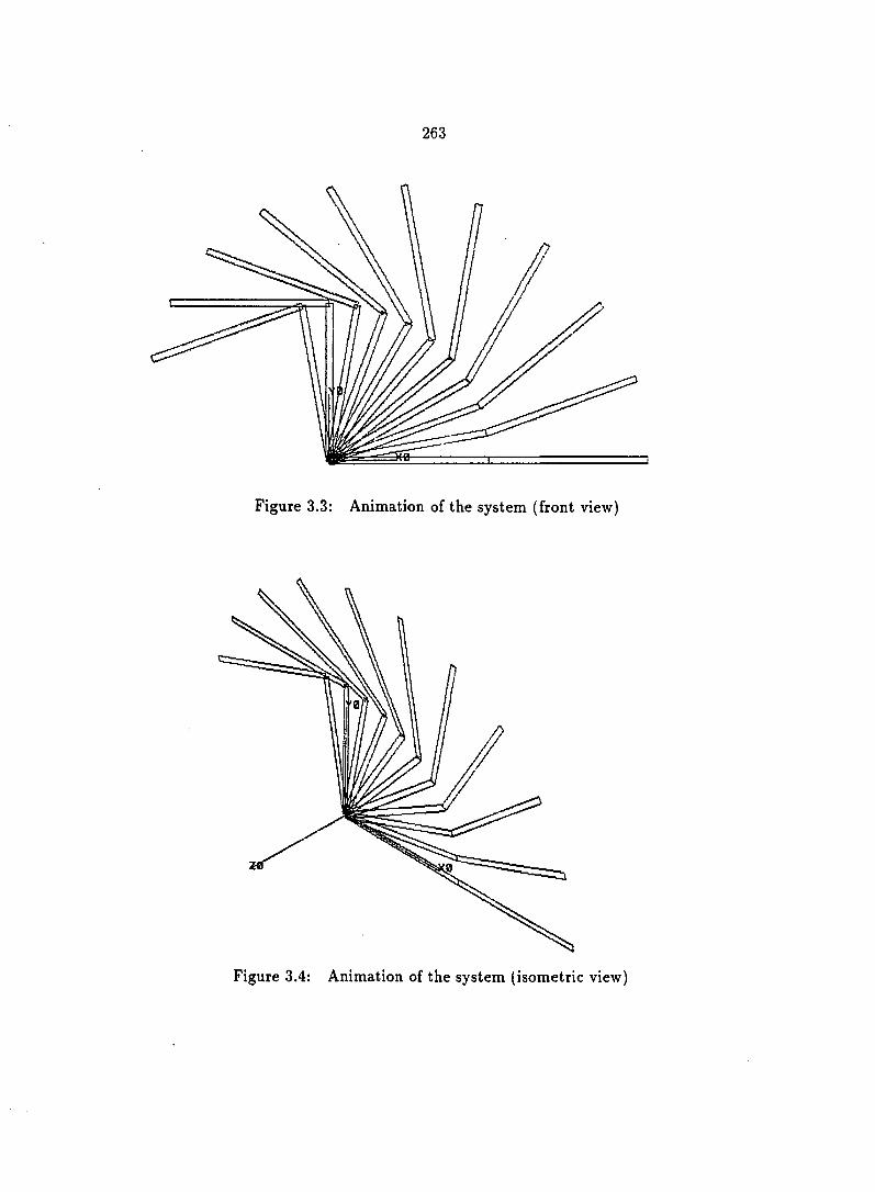
263

Figure 3.3: Animation of the system (front view)

Figure 3.4: Animation of the system (isometric view)

264

30

20

5 i i g

-10

-20

-30

0 40 60 20 80 100

ROTATIONAL ANGLE (DEC.)

Figure 3.5: Driving torque at joint one

40 60

ROTATIONAL ANGLE (DEC.)

100

Figure 3.6: Driving torque at joint two

265

n POSTl -INP» POSTl -INP"

nr<THFHWTPILflTflR (P3TB) .nmHFhtfMTPIIftTTR

POSTl -INP"

iFlBiaf tYMRlATm <P2T3) nn(ta.g MANtmij^TOR (P«T7)

Figure 3.7: Elastic deflection at different configurations

266

Figure 3.8: Animation of system free vibration

267

-1.48

1.49

1.51

1.52

1.53

1.54

1.55

-1.56

-1.57

-1.58

-1.59

—1.6

1.61

1.62

-1.63

-1.64

-1.65

-1.66

0 2 3

TIME (a) • FLEXIBLE + RIGID

Figure 3.9: Numerical solution of joint one

0.07

0.06

0.05

0.04

0.03

0.02

0.01

0.01 -

-0.02

-0.03

-0.06 2 3 4 0 1

TIME (•) • FLEXIBLE + RIGID

Figure 3.10: Numerical solution of joint two

268

-2 -

—3 -

0 2 3 4 1

TIME (m.)

Figure 3.11: Elastic deflection of point mass

1.4

0.8 -

0.6 -

0.4 -Z o"

0.2 -

—0.6 -

—0.8 -

-1

-1.2 -

-1.4

0 1 2 3

HME (•.)

Figure 3.12: Elastic deflection of point mass mo

269

Example 2: Mobile Crane Problem

A mobile crane in a working situation as shown in Figure 3.13 is studied as a

second example to demonstrate the application of the unified 4x4 transformation

matrix approach in formulating the system equations of motion. The crane has a

rigid-body chassis with four flexible outriggers. A rigid rotary support is attached

to the chassis, and the flexible boom is assumed to be supported at the end of the

rotary column [7-13].

The orientation of the crane body is represented by a local coordinate system

with the origin located at the mass center of the crane body. A global

coordinate system (XVZ) is defined to be parallel to the local coordinate system

with the origin located on the inertia space. The crane body is assumed to have

vertical (bounce) motion and roll and pitch motion about the mass center of the

crane body (as shown in Figures 3.14 and 3.15). The vertical motion of the crane

body is related to the global coordinate system by a 4 x 4 transformation matrix in

the form: •

X 1 0 0 0 X I

Y 0 1 0 y <

h

Z 0 0 1 0

1 0 0 0 1 1

The position vector for the mass center of the crane body in the global coordinate

system is expressed in the form:

Ac = yV (3.30)

The linear velocity of the crane body in the vertical direction is obtained by the time

Figure 3.13: Mobile crane at work

mb3

me

Krr

Figure 3.14: Schematic drawing of the crane model

v-pm

% 4

xb

X4

boom pivot

1 2

J3 J4

^ ïlboom^ slide

to to

Figure 3.15: Definition of local coordinate systems

273

derivative operation and is expressed in the form;

R c = y Y (3.31)

(3.33)

The roll and pitch motion of the crane body are assumed to be small. The angular

velocity of the body is represented in the local coordinate system in the

form:

uc = ax i+ i3z i (3 .32)

The pivot point of the lifting boom relative to the mass center of the crane

body is determined by introducing some intermediate local coordinate systems. The

location of the vertical rotational joint is represented by a local coordinate system

(22^2-2) relative to the body coordinate system in a matrix form:

1 0 0

0 1 0 Ar

0 0 1 0

0 0 0 1

where L3 is the longitudinal distance between the vertical rotational axis and the

mass center; hr is the vertical distance of the origin of the rotational joint relative to

the mass center of the crane body.

The swing motion of the boom is modelled by considering the relationship be­

tween two coordinate systems (z2#2^2 ^3^3-3) ^ matrix form:

cos#! 0 sin 0

0 1 0 0

— sin 0 cos 6-^ , 0

0 0 0 1

•^1

n ' ---

h 1

®2

<

=2

1

'

^2

h

-2

1

'3

n <

-3

1

(3 .34 )

274

'

®3

h

-3

1

'

i/4 <

H

1

(3.35)

where 9-^ is the swing angle about vertical rotational axis. For different operation

positions, the angle varies in the range from 0° to 360°. The end support of the

boom is located on the rotary part and is represented by the local coordinate system

(54^454) relative to the coordinate system in the form:

1 0 0 — ^ 4

0 1 0 &&

0 0 1 0

0 0 0 1

where and hj^ are the longitudinal and vertical distances between the origin of the

vertical rotation and the horizontal pivot point of the boom, respectively. The lifting

position of the boom is represented by the rotational angle of the local coordinate

system {x^^y^z^) attached on the end of the boom relative to the coordinate system

(54^454) in the form:

cos $2 — sin ^2 0 0

sin 62 cos ^2 0 0

0 0 1 0

0 0 0 1

where 62 is the lifting angle of the boom. By controlling these two rotational angles,

6^ and ^2, the operator could move the boom into the desired position. These two

variables are used as inputs for the computer simulation of the kinematic motion

analysis of the boom. Three sections of booms are used in the model: the first

section is connected to the pivot axis and is used to determine the lifting angle of the

entire boom; the second and third sections are allowed to move along the slot and get

the required length of operation. Two variables, J3 and J4, are used to represent the

'

.T4

U

-4

1

H n

<

~b 1

(3.36)

275

position of the two outreach booms. A computer model for the simulation package,

IMP, has been developed to represent the mobile crane working positions.

Figures 3.16 and 3.17 show the initial position of the mobile crane in a side view

and an isometric view, respectively. The crane body is modelled to have a vertical

translational motion about the local axis and two rotational motions about local

XI and zi axes. The system is supported by four outriggers on the level surface. The

rear lifting operation is modelled and shown in Figures 3.18 and 3.19 for side view

and isometric view, respectively. During the lifting operation, the boom is extended

by controlling the joint motion of the outreach booms. The top view of the boom

swing motion is shown in Figures 3.20. Figure 3.21 shows the boom swing motion

around the rear end in an isometric view.

The operation of the crane in the swing motion introduces the centrifigal force

on the boom, the sudden start and stop of the swing motion result in the the lateral

inertia forces on the boom. In this study, the crane body is allowed to have vertical

motion and roll and pitch motion about the mass center of the crane body. The

vertical motion is animated in Figure 3.22, the roll motion about the mass center of

the crane body is shown in Figure 3.23 and the pitch motion is shown in Figure 3.24.

The movement of the boom changes the location of the overall mass center of

the crane body and the direction of the inertia and centrifugal forces. Dynamic

equations of motion are formulated with the swing and lifting position of the boom

being assumed as known input variables. The flexibility of the boom is considered in

dynamic equations. The elastic deformation was modelled by considering the boom

as a cantilever beam with different cross section areas. The vibrational mode shapes

were computed by using finite element method. The first three transverse vibrational

cC

1.

n t) a to

Figure 3.16: Side view of the initied position

m

>>•

Figure 3.17: Isometric view of the initial position

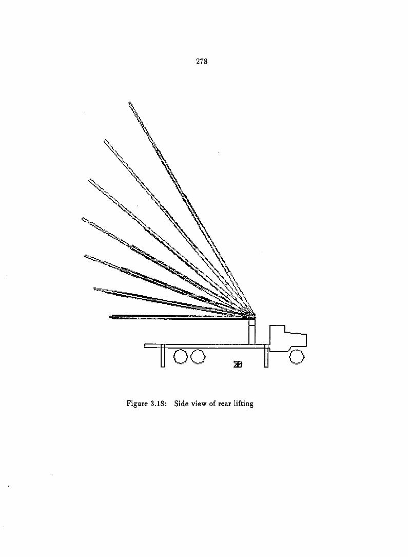
278

Figure 3.18: Side view of rear lifting

279

Figure 3.19; Isometric view of rear lifting

Figure 3.20: Top view of boom swing motion

281

Figure 3.21: Isometric view of swing motion

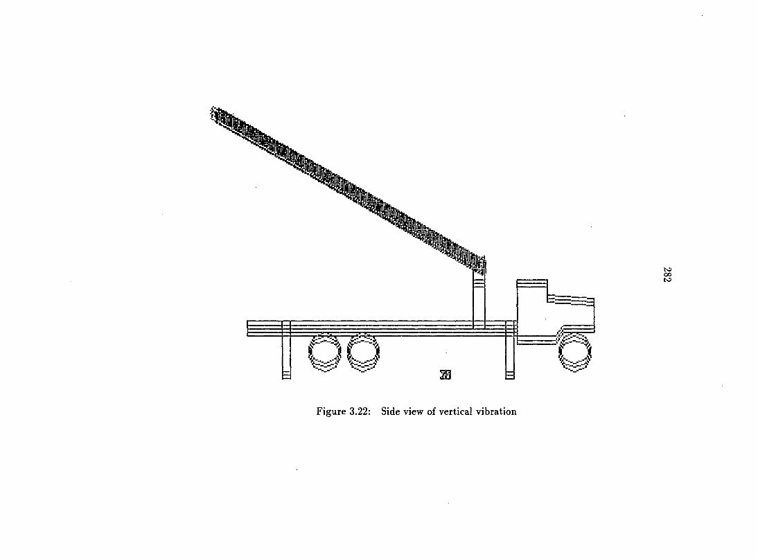
Figure 3.22: Side view of vertical vibration

Figure 3.23: Front view of roll vibration

Figure 3.24: Side view of pitch vibration

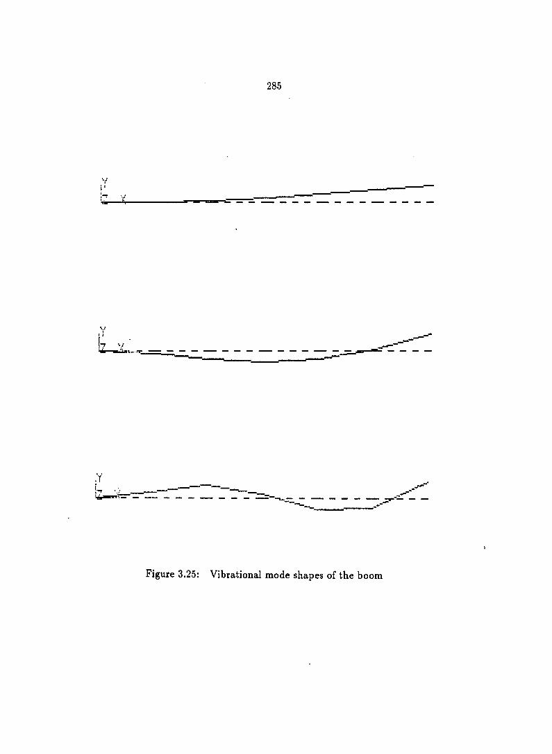
285

Figure 3.25: Vibrational mode shapes of the boom

286

modes of the boom extended in full length are shown in Figure 3.25. To simplify the

formulation of system equations of motion, the boom is modelled with three lumped

point masses located at the end of each section. The local coordinate system

is used to measure the local position of the point masses. The position vector of the

point masses in the local coordinate system is expressed in the form:

''61 =

hi h2 hz «1

< II «2 11 "3

("1 n ^3

1 1 1

(3.37]

where Uj and are the vertical and lateral elastic deformation of the boom at the

location of the ith point mass, is the longitudinal distance between the point

mass and the origin of the local coordinate system at the pivot point of the support

end.

Three modes are used to represent the elastic deflection of the boom in vertical

and lateral directions, respectively:

+ i2yV2i^) +

= *ilz^l(0 + *i2z^2(^) +

(3.38)

(3.39)

or in matrix form:

%1 *11% *12% *13% V I

"2 *21% *22% *23% < V 2

, ^3 . . *31% *32% *33% . . % .

(3.40)

287

n *llz *12; $13z

*21z $22z $23z < (2

. "3 , $31z *322 *332 f3 ,

where ^{jy and are determined from the jth vibrational mode shape at the

ith point mass in the vertical and lateral directions, respectively. Vji^) and ^j{t) are

the jth modal variables. With modal variables, accurate information of the elastic

boom is obtained and yet fewer degrees of freedom are needed if more point masses

are used to model the boom. For this simplified example, the advantage of using

mf^dal variable instead of actual displacement variable is not very obvious because

only three point masses are used to model the boom.

The position of the point mass, in the local coordinate system on

the crane body is obtained through consecutive matrix multiplications in the form:

1 0 0 H

0 1 0 hf

0 0 1 0

0 0 0 1

1 0 0 -L

0 1 0 h

0 0 1 0

0 0 0 1

cos Oi

0

- sin $1

0

cos $2 — sin ^2

sin $2 cos 02

0 0

0 0

0 sin 9^ 0

1 0 0

0 cos 0

0 0 1

0

0

1

0

0

0

0

1

' 'bi

288

cos cos ^2 — cos0]^sin02 sin^^ X3 — ^4 cos 9i hi

sin ^2 cos 2 0 hb + hr <

"i >

— sin 9^ cos 2 sin 9-^ sin ^2 cos 9-^ sin "i

0 0 0 1 1

= COS COS ^2 — Uj COS sin $2 + i^i sin 6i + cos 6^ |

+ y I sin $2 + %% cos ^2 + '^è + }

+ 5]^ {~^bi cos 62 + Uj sin 9-^ sin 2 + cos 9^ + Z4 sin^j^j

= [Z-p j — u j cos 9^ sin ^2 + sin 0]^]

+ + «icos02]

+ c]^[JD.j + Uj sin sin ^2 +cos 0]^] (3.42)

where Lyi and L~i are known dimension parameters in the longitudinal, vertical

and lateral directions of the crane body, respectively, and are defined in the forms:

^xi — ^3 ~ ^4 cos 9i + cos 9i cos 2 (3.43)

^yi - + L^i sin ^2 (3.44)

Lzi — ^4 sin sin^^ cos 2 (3.45)

The absolute velocity of the point mass on the boom is obtained by considering

the general motion of the crane body, the relative motion of the boom in vertical and

lateral directions, the effects of the angular velocity of the crane body on the boom,

and is expressed in the form;

Vfji = Rc + Rii +W1 X

289

= ïq cos sin ^2 + sin^i — ^{Lyi + cos #2)]

+ y I [y + "i cos 62 + 0(^22 - u j cos 91 sin O2 + sin )

—à[L~i + xii sin 9i sin 2 + cos O-^ )]

+ sin^]^ sin 2 + cos + a(Ly,j-+ cos ^2)] (3.46)

Since the length of the boom is much greater than the elastic deflection, the addition

of deflection to the length of the boom is insignificant. Thus, the velocity equation is

further simplified by ignoring some insignificant terms in the dimension of the system

and is expressed in the form:

^hi ~ cos 61 sin ^2 + sin — ^Lyi]

+ n[y + cos gg + ^Lxi -

+ 5]^[ûj sin sin02 +cos + âZyj] (3.47)

With the velocity expression for the point mass on the boom, the kinetic energy

of the system is computed by considering the motion of the crane body in the vertical

direction and the roll and pitch motion and the elastic deflection of the point mass

on the boom. The system kinetic energy is expressed in the form:

T = -mcil^ + -Ixxôi^ + -Izz0^

+ 2 ^ [•"! + +y^ + + ^ii) + + ^yi) i = l

+'2ii j^l3{Lyi cos $1 sin ^2 + cos 62) + cos

+1ùià[Lyi sin 9i sin ^2 — cos ^2 ) - 2ùj^j3Lyi sin

+2ywj cos 92 + '2y^L^i - 2yàL^i - (3.48)

where Ixx and Izz are the moments of inertia of the crane body for the roll and pitch

290

motions, respectively. The potential energy of the system is obtained by considering

the strain energy of the outriggers, the strain energy of the boom and the effects of

the gravity acceleration, and is expressed in the form:

^ = 2^fl^y ~ 6" + ^2/))^ + + -^6" + ^2/))^

+ 2^rl^y ~ 5°: ~ -^1/5)^ + 2^rr{y + L^a — Lij3)^

1 + r

V I T

4i A'l2 ^13 V I 1

+ r V 2 •

4i 42 43 < V 2

. ^3 . . 4i 42 4 3 . , ^3 ,

T • / \

A'fl A'fg

(2 ^21 ^22 % (2

. ^3 . . % % 3 3 . , ^3 ,

3 + rricgy + ^ ( i/ + L i + cos

i=l 3

+ - "i cos 9i sin 62 + vi sin ) ( = 1

— a ( I - j + U j s i n ^ ] ^ s i n ^ 2 + c o s ( 3 . 4 9 )

where g is the acceleration of gravity; and AVr are the equivalent

stiffnesses of the supporting outriggers in the front, rear, left and right positions

of the crane body, respectively; A'f- and Kf- are the modal stiffness of the boom

corresponding to the vertical and lateral vibrations, respectively.

The generalized applied forces due to centrifugal force of the boom in rotational

motion are obtained using the virtual work principle. The virtual work due to rota-

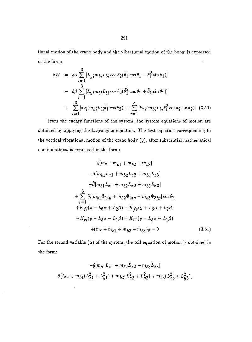
291

tional motion of the crane body and the vibrational motion of the boom is expressed

in the form:

3 8W = 6a Y, [Lyi '^hihi cos h " sin )]

i=l 3

- Y [Lym^bi cos 2(^1 cos + ^'1 sin é»!)] i=l

3 . 3 + Z cos ^2)] - Y1 i^ni^bihih COS &2 sin 2)1 (3-50)

i=l i=l

From the energy functions of the system, the system equations of motion are

obtained by applying the Lagrangian equation. The first equation corresponding to

the vertical vibrational motion of the crane body (j/), after substantial mathematical

manipulations, is expressed in the form:

y [ m c + + "^63!

-a[mbiL^l + m^2-^z2 + "^63 "^-3^

+i^[^bl^xl + '^b2^x2 + "^63-^2:3] 3

+ E nilmii^iiy + rnjj2^2iy + 63^3iy] cos^2 i = l

+ ~ ^6°^ + ^2!^) + Kfr^y + L^a + X2/3)

~ -^5^ ~ ^1/^) + I '>-rr{y + L^a — L-^jS)

+(mc + + m^2 + "^63)5 = 0 (3.51)

For the second variable (a) of the system, the roll equation of motion is obtained in

the form:

-y[^b\^z\ + b2^z2 + "^63^-3]

a [ I x x + + i y i ) + 1 ^ 6 2 + ^ 2 ) + 6 3 ( ^ z 3 + y 3 ^ î

292

-i^b^bl^xl^zl + b2^x2^z2 + 3

+ IZ ["1^1(^1/1 sin sin 2 - COS ^2)^1^2/ i= l

+"^62(^2/2 sin sin gg - z2 cos 2)^2iy

+"^63(^2/3 sin ^1 sin ^2 " z3 cos 2)^3zy]

3

+ Z + "^b2^y2^2i2 + "^63S3^322]cos^1 i = l

-^f i^eiy ~ + -^-2^) + fr^eiy + -^6" + ^2/^)

~ -^S*^ ~ -^l/^) + KrrL^{y + — Li/3)

—mi,ig(L~i + -uj^ sin^2 sin 2 + cos^j^)

-m^25(^-2 + "2 sinsin 2 + (^2 cos 0j)

—m^2,g[L2"^ + «3 sin sin ^2 + cos 2)

^ •• -2 = Z! (•^m"^6i'^6i)cos6'2(^l cos(9i - i9j sin(9i) (3.52)

i= l

For the third variable { j 3 ) corresponding to the pitch motion of the crane body, the

equation of motion is obtained in the form:

y['^h\^x\ + h2^x2 + "^63^z3i

-^[^bl^xl^zl + b2^x2^z2 + 63^z3^:3]

+i3[Izz + mbiil'^i + ^1) + "^62 (^y2

+LI2) + bZ^^yZ + ^z3)]

3

+ Z [^61 (^1/1 cos^i sin02 + cos02)^liy i = l

+^b2^Ly2 cos sin $2 + Ly,2 cos g2)$2i%/

^63(^2/3 cos Oi sin B2 + I^g cos 2)^3%%,]

293

3

- E + b2^y2^2iz + "^63^y3*3iz] sin^i 2 = 1

+^fl^2iy ~ 6°^ + ^2(3) + Rj:J .L2{Y + LQŒ + L2l3)

~ ^5^ ~ ^1(3) — KrrLi{y + L^a — Li0)

+mi^-^g{L^l — ui cos 9^ sin O2 + ui sin 6^ )

+m^29{ x2 ~ 2 ^1 ^2 + '^2 ^1 )

+"^63^(^z3 - 3 cos 1 sin 62 + 1/3 sin ) 3

= - E(^2/î"^6i-^6i)<^os02(^lco®^l + ^1 sin^^) (3.53) i= l

For the ith transverse vibration of the boom (rjj), the equation of motion is obtained

in the form:

vl^bl^Uy + b2Hiy + "^63^3i'i/] cos h

+à[m^l{Lyi sinélj sin6*2 - I-i cos6i2)^h-y

+ b2i^y2 sin^2 " z2 cos^2)^2%%/

+^63(^1/3 sin^i sin02 " =3 cos 2)^3i%/

i^l^bli^yl cos^i sin ^2 + xl cos ^2)^l«i/

+m62( Ly2 cos 01 sin ^2 + z2 cos O2 )^2iy

^63(^2/3 cos sin ^2 + ^r3 cos 2)^3;y]

+Vl[mi,i^l ly^liy + mij2^21y^2iy + 63^31j/^3it/]

+V2{^bl^l2y^liy + '^b2^22yHiy + '"63^32y^3iyl

+n[^bl^lZy^liy + b2^2Zy^2iy + "^63^33y^3ij/l

-(asin^isin02 +/^cos0isin02)(^liy"^6l +^2zi/"^62 + %y"^63)

294

3

+ E ) + (mi^1/3/ + "^62^2iy + '^hzHiy)9 cos 2 J=1

= + TT^b2h2^2iy + "^fe3^63^3iy) cos 2^1

i = 1, 2, 3 (3.54)

The vibrational motion in the lateral direction of the boom corresponding to the

modal variables (^j) is obtained in the form:

+ "^62^2/2^2Z"Z + "^63^2/3^3ir] cos

-f3[mbiL.yi^^ - . + mi,2^y2^2iz +

+^lk61^11z^liz + "^62^21z^2i'z + '"63^31z^3iz]

+&[mi^l2z^hz + m2^22z*2iz + "^63^32z^3iz]

+^3["^6l^l3z^liz + "^62^23z^2iz + "^63^33z^3izl

+ K^2^2 + 'i3^3

+(13 sinei - acos0i)($ij-mji + $2iz"^62 + 3iz^63)

= kil^èl^liz + b2^b2^2iz + "^M^63^3iz]^l cosgg

i = 1, 2, 3 (3.55)

The symmetry of the mass matrix for these equations is observed. The system equa­

tions of motion are integrated to conduct dynamic analysis of the system from known

initial conditions and given design parameters.

The dynamic response of the system was studied at a selected operation condi­

tion. The parameters of the system were estimated based on the SAE Standards and

related literatures, and are listed in Table 3.2.

295

Table 3.2: Parameters of the mobile crane

Description Value Mass of the crane body (mg) 15000 kg Mass of the first point mass 1150 kg Mass of the second point mass (m^2) 952 kg Mass of the third point mass 752 kg

Roll moment of inertia ( I x x ) 1.2E5 kg-m?

Pitch moment of inertia { I z z ) 1.5E5 kg-m^ Longitudinal location of rear outriggers [L^] 4.0 m Longitudinal location of front outriggers (£2) 1.8 m longitudinal location of vertical pin (L3) 1.0 m Horizontal offset of boom pivot (£4) 0.35 m Lateral location of rear outriggers (£5) 2.5 m Lateral location of front outriggers (Lq) 2.6 m Height of supporting column [ h r ) 1.2 m Height of boom pivot (/ij) 0.4 m Location of the first point mass ) 8.0 m Location of the second point mass (£^2) 16.0 m Location of the third point mass (£53) 24.0 m Stiffness of front outriggers ( K 5.4E5 N/m

Stiffness of rear outriggers { K ^ i , K r r ) 4.8E5 N/m

Boom cross section area of section one 1.84E-2

Boom cross section area of section two (^2) 1.52E-2 m2

Boom cross section area of section three ( .A3) 1.20 E-2 Bending stiffness of section one 4.46E7 N-m^

Bending stiffness of section two ( E I 2 ) 2.65E7 N-m2

Bending stiffness of section three [ E I ^ ) 1.40E7 N-m2

296

The position with the swing angle of 45° from the front end of the crane body

and the lifting angle of 60° from horizontal plane (as shown in Figure 3.26) was used

for the dynamic analysis of the system. The boom was assumed to have a constant

swing motion at the rate of 2 revolution per minute. The angular acceleration of the

boom in swing motion is assumed to be zero, the lateral deformation was ignored

in the numerical solution. The elastic deflections of the boom under gravity effects

of the point masses and centrifugal forces at different lifting angles (45°, 60°, 75°)

were computed using finite element method and were shown in Figure 3.27.

The vertical vibration of the crane body was simulated by releasing the system

from the position with zero vertical deflection of the outrigger springs. The system

equations of motion were integrated by considering the different vibrational modes

of the boom. Figure 3.28 shows the vertical vibration of the crane body for a rigid

boom and a flexible boom with one vibrational mode. The introduction of the first

vibrational mode of the boom does not have significant effect on the vertical vibration

of the crane body. Figure 3.29 shows how the vertical vibration of the crane body is

affected by using one, two and three vibrational modes of the boom. The inclusion

of the first two modes of vibration significantly affected the vertical vibration of the

crane body. With three modes of vibration, the vertical response does not change

much as compared to the result from using the first two modes. This suggests that

the use of only one mode underestimates the flexibility effects of the boom on the

vertical vibration of the crane body, but the use of two modes of vibration produces

a satisfactory result.

The roll motion of the crane body was simulated with different vibrational modes

of the boom being used. The dynamic response of the roll motion was integrated from

297

Figure 3.26: Boom bosition for dynamic analysis

298

Figure 3.27: Elastic deflection of the boom

299

rigid boom and flexible boom behavior with one vibrational mode. The eff'ects of the

boom flexibility on the roll motion of the crane body are shown in Figure 3.30. The

introduction of boom flexibility with one mode has slightly changed the roll motion.

Figure 3.31 shows the flexibility effects of the boom with one, two, and three modes of

vibration on the roll motion of the crane body. The use of one mode underestimates

the flexibility effects. The use of two modes gives results similar to using three modes,

which means that the addition of third mode to the first two does not significantly

affect the roll motion of the crane body.

The pitch motion of the crane body was studied in the same manner by com­

paring the results from rigid boom and flexible boom analysis with different modes.

Figure 3.32 shows the pitch motion of the crane body under the condition of rigid

boom and flexible boom with one vibration mode. The introduction of boom flexibil­

ity with one mode does affect the pitch motion of the crane body, but the vibration

frequency is almost the same as for the rigid boom. The use of two vibrational modes

of the boom has a significant effect on the pitch motion of the crane body. The results

computed with three modes of vibration agree well with the results from using the

first two modes, as shown in Figure 3.33.

The elastic deflection of the boom at the location of each point mass was com­

puted by considering each vibrational mode of the boom. Figure 3.34 shows the

elastic deflection at different locations computed from the first mode of vibration.

The displacement at different points has the same phase as expected from the first

mode shape of vibration. The magnitude of defiection at the end is much greater

than that at the middle points of the boom. Figure 3.35 shows the elastic deflection

at the different points on the boom computed from the second mode of vibration.

300

The deflections at two middle points are in the same phase with almost the same

magnitude. The deflection at the end of the boom is in the opposite direction with

the magnitude being twice as much as that on the other two points.

The elastic deflection of the boom computed from the first two modes of vibration

is shown in Figure 3.36. The two modes have different frequency and mode shapes.

The deflection at is in the opposite direction from the deflection in and

has a much smaller magnitude. The location of the is close to the node of the

second mode of vibration, and the two modes cancel each other at that point. The

elastic deflection is then much smaller than the deflection at the end of the boom.

The utilization of two modes has greater effect on the elastic deflection than the use

of either mode separately. Figure 3.37 shows the elastic deflection at different points

with three modes of vibration. The addition of the third mode does not signiflcantly

affect the elastic deflection of the boom, which indicates that using two modes will

produce satisfactory results.

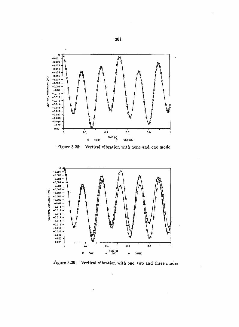
301

FLEXIBLE

Figure 3.28: Vertical vibration with none and one mode

0 0.2 0.4 0.6 O.B 1

TIME (a) • ONE + TWO O ThREE

Figure 3.29: Vertical vibration with one, two and three modes

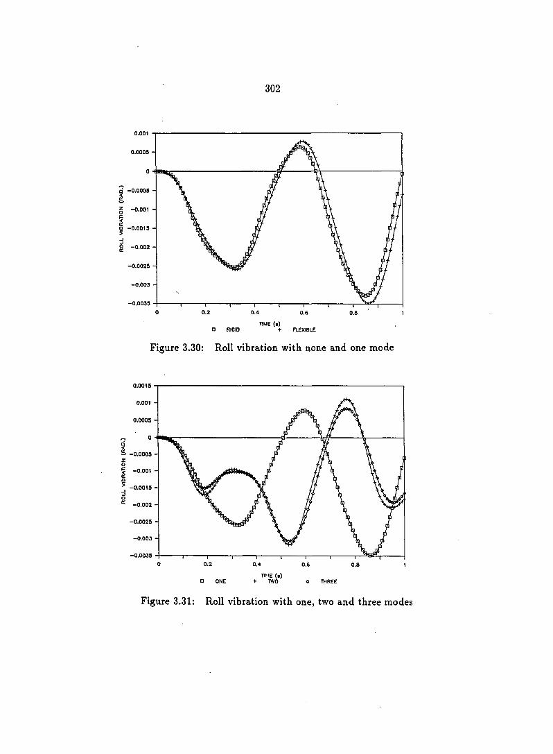
302

0.001

0.0005 -

a -0.0005 -

Z -0.001

S -0.0015 -

•0.002 -

-0.0025 -

—0.003 -

•0.0035

0 0.2 0.4 0.6 0.8 1 TIME (a)

• RIGID + FLEXIBLE

Figure 3.30: Roll vibration with none and one mode

0.0015

0.001 -

0.0005 -

^ -0.0005 -Z

0.001 -

-0.0015 -

0.002 -

-0.0025 -

-0.003 -

0.0035 -

TtME (a) TWO

Figure 3.31: Roll vibration with one, two and three modes

303

0.0005

-0.0005 -

-0.001

•0.0015 -

5 -0.002 -

-0.0025 -

-0.003 -

-0.004 -

-0.0045

0 0.2 0.4 0.6 0.8 1 TIME (a)

Q RIGID + FLEXIBLE

Figure 3.32: Pitch vibration with none and one mode

0.0005

-0.0005 -

—0.001 -

^ -0.0015 -

-0.002 -

-0.0025 -

—0.003 -

-0.0035 -

—0.004 -

-0.0045

0 0.2 0.4 0.6 O.B 1

TIME (#) Q ONE + TWO 0 THREE

Figure 3.33: Pitch vibration with one, two and three modes

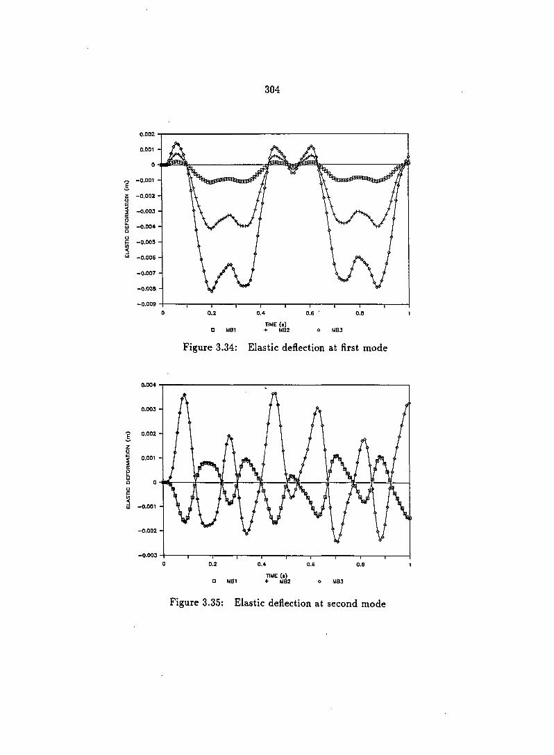
304

0.002

0.001 -

-0.001 -

0.002 -

0.003 -

-0.005 -

-0.006 -

-0.007 -

0.008 -

-0.009

TIME (a) MB2 • MB1

w —0.004 -o

Figure 3.34: Elastic deflection at first mode

0.004

0.003 -

0.002 -

0.001 -

(J —0.001 "

-0.002 -

•0.003

0 0.2 0.4 0.6 0.8 1

TIME (•) • MB1 + MB2 o MB3

Figure 3.35: Elastic deflection at second mode

305

0.08

0.06

0.04

0.02

J11 m 111111 >0.02

•0.04

•0.06

•0.08

•0.1

•0.12

•0.14

•0.16

•0.18

•0.2

•0.22 0.4 0.6 0.8 0 0.2 1

TIME (») • MB1 + MB2 o MB3

Figure 3.36: Elastic deflection with two modes

TIME (,)

Figure 3.37: Elastic deflection with three modes

306

Example 3: Front-end Loader Problem

A front-end loader is used to transport a heavy load to a desired height and

position. There are different linkage designs to accomplish this function [14-18]. The

basic structure of the loader consists of a mobile chassis mounted on wheels to carry

the object from one place to another and a linkage system which is controlled by the

hydraulic cylinder to get the bucket to the desired height and angular position. The

linkage is a closed-loop mechanism. A Ford/New Holland model L555 was discussed

in this example to demonstrate the application of computer simulation for closed-loop

mechanical systems.

The linkage system (as shown in Figure 3.38) consists of a lifting arm which

provides the support for the bucket at the end, a lower lift link which controls the

lower end of the lifting arm by rotating about a fixed pin on the chassis, an upper lift

link which controls the upper end of the lifting arm, a tilting cylinder used to control

the angular position of the bucket relative to the lifting arm, and a lifting cylinder

to drive the entire linkage system.

The kinematics of the linkage was studied by considering the geometric con­

straints of the upper and lower links and the driving position of the lifting cylinder.

Computer simulation provides a practical means to study such a system. It is difficult

and time consuming to study the closed-loop mechanical system by traditional man­

ual calculations. In this study, an Integrated Mechanisms Program (IMP) was used

to analyze the kinematic performance of the linkage. The linkage was modelled by

setting up two local coordinate systems on two adjacent links at the same joint. The

number of independent loops of the system was computed by determining the rank

of the geometric constraint matrix. For this example, three independent loops were

LLAPT

Chassis

-Upper lift link

•UCPT

Llftarm

UTCPT

Tilt cylinder (TCYL)

LTCPT

ULCPT

ULAPT

LLCPT

Lower lift link

Bucket

BKPT

LCPT

Lift cylinder (LCYL)

oa O —Ï

Figure 3.38: Ford/New Holland front-end loader system

308

observed. The first loop was the bucket position control loop containing the joints:

BKPT-LTCPT-TCYL-UTCPT-BKPT. The second loop was the lower lifting mecha­

nism loop containing the joints: LCPT-LLAPT-ULCPT-LCYL-LLCPT-LCPT. The

third loop was the upper position control mechanism loop containing the joints:

LCPT-LLAPT-ULAPT-UCPT-LCPT.

The kinematic analysis for the loader was conducted to study the motion of the

bucket. Figure 3.39 shows the initial position of the system. Figure 3.40 shows the

rotational motion of the bucket about the pin joint at the end of the lifting arm. The

angular position of the bucket was controlled by the tilting cylinder.

The height of the bucket was controlled by extending the driving cylinder while

the upper and lower links provided the orientation control over the lifting arm. Fig­

ure 3.41 showed the lifting operation driven by the lifting cylinder. The path of the

bucket was shown clearly through the simulation. The design modification was an­

imated by changing the configuration of the linkage. The horizontal motion of the

chassis was modelled by introducing a prism joint between the terrain and the chas­

sis. The animation of such horizontal motion of the system is shown in Figure 3.42,

and the dumping operation of the bucket is shown in Figure 3.43

When the load inside the bucket was assumed to be 4.4482 kN, the force required

to tilt the bucket was determined through the simulation process and is shown in

Figure 3.44. The force required by the lifting cylinder was also determined and is

shown in Figure 3.45. The pressure requirement of the hydraulic cylinder could be

calculated from the axial force requirement, which provided the necessary information

for the proper design of the linkage.

The elastic deflection of the lifting mechanism was studied using the finite ele-

309

ment method. The linkage was modelled as beams with each member being assumed

to have a uniform cross section area. The initial configuration of the linkage is shown

in Figure 3.46. The chassis of the loader was assumed to be rigid and was plotted to

show the boundary condition for the linkage systems and to show the relative posi­

tion of the linkage with respect to the chassis. The elastic deflection of the linkage

at three different positions is shown in Figures 3.47, 3.48 and 3.49.

so

Figure 3.39: Initial position of the linkage

zo

Figure 3.40: Rotational motion of the bucket

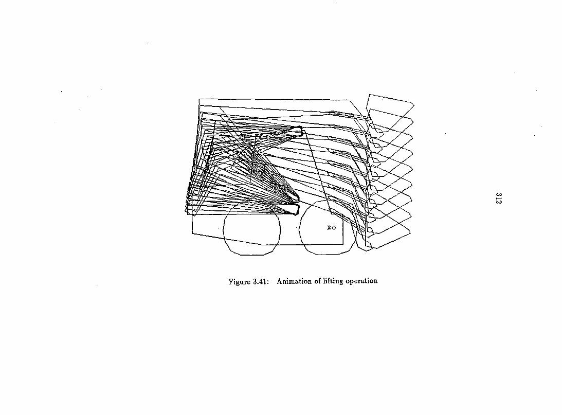
Figure 3.41: Animation of lifting operation

Figure 3.42: Animation of chassis horizontal motion

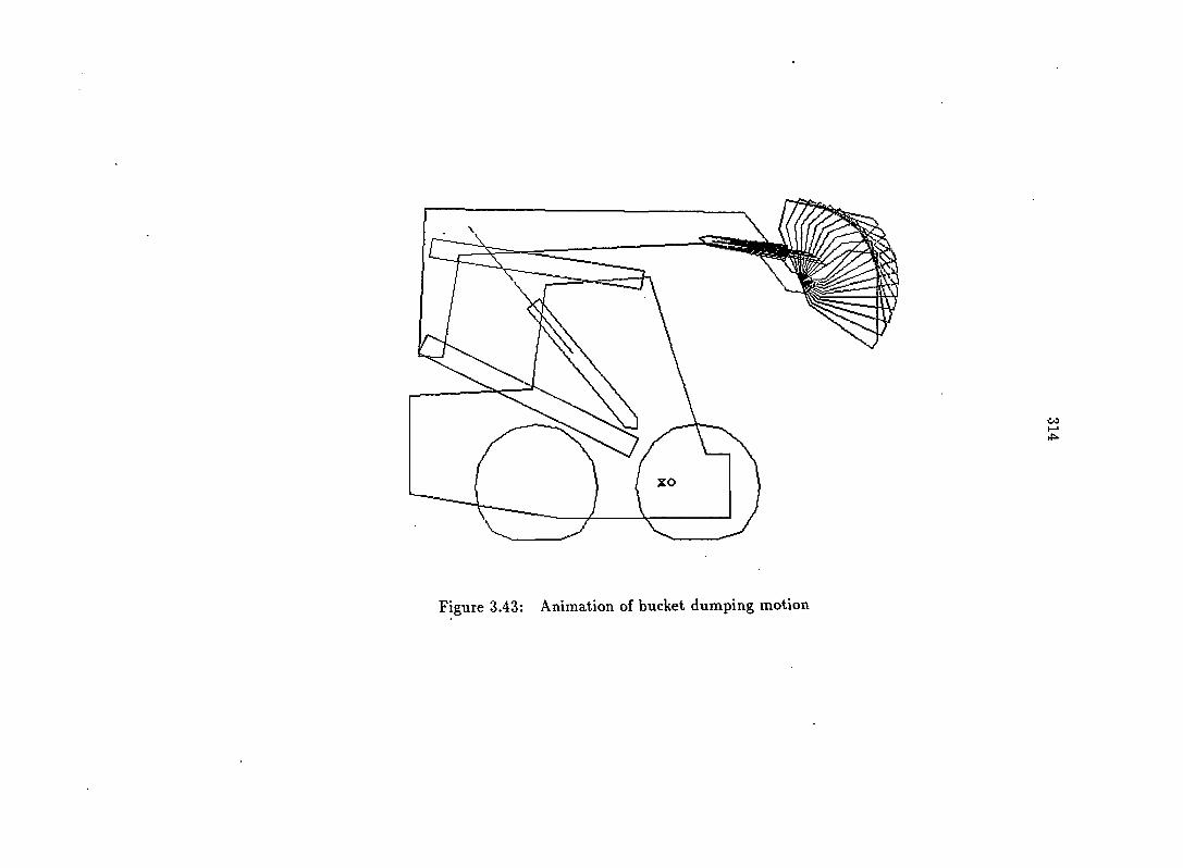
Figure 3.43: Animation of bucket dumping motion

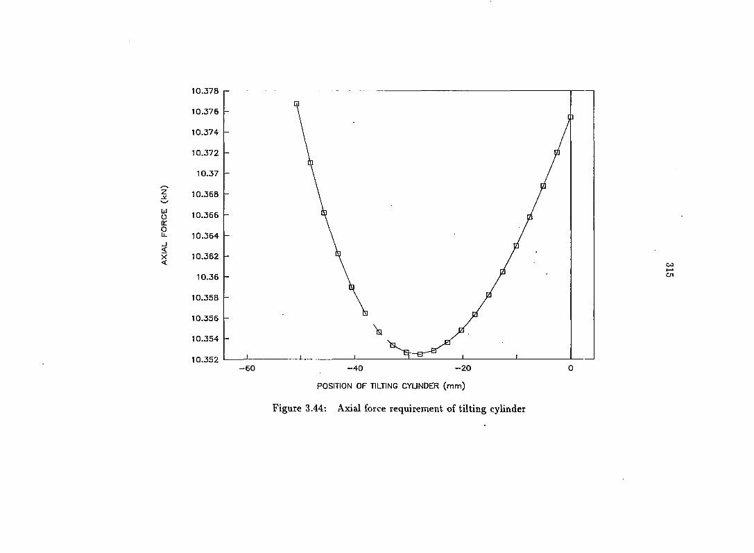
10.378

10.376

10.374

10.372

10.37

10.368

10.366

10.364

10.362

10.36

10.358

10.356

10.354

10.352 -20 0 -60 -40

POSITION OF TILTING CYLINDER (mm)

Figure 3.44; Axial force requirement of tilting cylinder

14-.1

13.9

13.8

13.7

13.6

13.5

13.4

13.3

13.2

13.1

12.9

12.8

12.7

12.6

12.5

12.4

12.3 -

12.2 -

12.1 -0 20 40 60

LIFTING CYLINDER POSITION (cm)

Figure 3.45: Axial force requirement of lifting cylinder

317

Figure 3.46: Initial position of the lifting system

Figure 3.47: Deflection of lifting system at lower position

318

Figure 3.48: Deflection of lifting system at middle position

,)—

Figure 3.49: Deflection of lifting system at upper position

319

CHAPTER 4. SUMMARY

The algorithm for determining system equations for open and closed-loop me­

chanical systems was formulated based on the results of Part II. For an open-loop

mechanical system, the kinematic relationship of the linkage was determined in a

forward direction from the base support to the end, and the dynamic relationship

was determined backward. The recursive method to determine the inertia matrix

and the general force vector were defined. For a closed-loop mechanical system, the

kinematic analysis was conducted to determine the system degrees of freedom and

the relationship of dependent variables to independent variables. The equations of

motion were then formulated corresponding to the independent variables. The non­

linear, second order, differential equations were linearized to simplify the numerical

computation.

Three examples were used to demonstrate the basic modelling concepts and

simulation procedures for both open and closed-loop mechanical systems. The double

pendulum was modelled as an open-loop system. Assumed mode shape functions

were used to estimate the flexibility of the links. The step-by-step procedure and

simulation results demonstrated the flexibility effects of the links. The mobile crane

example extended the open-loop mechanical system by considering the motion of the

chassis in vertical, pitch and roll directions. The front-end loader was modelled as a

320

closed-loop mechanical system. The animation of the lifting operation was conducted

to determine the force requirement inside both tilting and lifting cylinders. The

simulation results provided the necessary information for designing the linkage and

position control of the system.

321

BIBLIOGRAPHY

Craig, J. J. 1989. Introduction to robotics: Mechanics and control. Addison-Wesley Publishing Company, New York.

Smith, J. D. 1989. Vibration measurement and analysis. Bitterwpr Butter-worths & Co. (Publisher) Ltd, London.

Barton, L. 0. 1984. Mechanism analysis: Simplified Graphical and analytical techniques. Marcel Dekker, Inc., New York.

Hall, A. S. Jr. 1966. Kinematics and linkage design. Bait Publishers, West Lafayette, Indiana.

Korein, J. U. 1985. A geometric investigation of reach. The MIT Press, Cam­bridge, Massachusetts.

Phillips, J. 1984. Freedom in machinery. Volume 1: Introducing screw theory. Cambridge University Press, Cambridge, London.

Kato, Y., and H. Ito. 1984. Study on dynamic stability of a truck crane carrier. 1st report: Backward stability of a carrier with outriggers. Bulletin of JSME 27:1251-1257.

Ito, H., M. Hasegawa, T. Irie, and Y. Kato. 1985. Study on dynamic stability of a truck crane carrier. 2nd report: Strict analysis of forward stability in load lowering motion. Bulletin of JSME 28:2467-2473.

Ito, H., M. Hasegawa, T. Irie, and Y, Kato. 1985. Study on dynamic stability of a truck crane carrier. 3rd report: Approximate analysis of forward stability in load lowering motion. Bulletin of JSME 28:2474-2479.

Dickie, D. E. 1975. Crane handbook. Construction Safety Association of On­tario, Toronto, Canada.

322

11] Shapiro, H. I. 1980. Cranes and derricks. McGraw-Hill Book Company, New York.

12] Kogan, J. 1976. Crane design: Theroy and calculations of reliability. John Wiley & Sons, New York.

13] Schwarz, H. R., J. R. Whiteman, and C. M. Whiteman. 1988. Finite Element Methods. Academic Press Inc., San Diego, CA.

14] JML Research, Inc. 1988. The integrated mechanism Program: Language Spec­ification and user's manual. JML Research, Inc., Madison, WI.

15] Hain, K. 1967. Applied kinematics. McGraw-Hill Inc., New York.

16] Claar, P. W., D. D. Furleigh, and D. R. Rohweder. 1986. Computer graphics for agricultural equipment simulation and design. SAE Paper 861293.

17] Claar, P. W. 1907. Simulation modelling of agricultural tractor performance of mobility. SAE Paper 872015.

18] Yan, J. H. 1988. Simulation of skid steer loader longitudinal stability and lift linkage performance. M.S. Thesis, Iowa State University, Ames, Iowa.

323

GENERAL SUMMARY

Dynamic principles used to formulate system equations of motion provide the

theoretical background for developing general-purpose computer simulation programs.

The vector dynamics (Momentum principle and d'Alembert's principle) has been

shown to provide a straightforward method to formulate equations of motion for

simple mechanical systems with little geometry complexity. The introduction of in­

teractive forces increases the complexity of formulating the system equations of mo­

tion. The energy method (Lagrange's equation and Hamilton Canonical equation)

eliminates the interactive forces in formulating the system equations. The derivative

operation of system energy functions becomes complicated and tedious for relatively

large mechanical systems. Kane's method provides a combination of both vector and

energy methods by introducing the vector-dot product approach and is ease to use

for open-loop mechanical systems.

The flexibility of mechanical system was modelled by introducing the flexible

link shape matrix. The system equations were formulated corresponding to both

large-displacement geometrically constrained motion and small magnitude elastic de­

flection. A unified 4x4 matrix approach was used to determine the system energy

functions. The equations of motion were developed systematically for open and

closed-loop mechanical systems.

324

The flexibility efl'ects during the large displacement motion were demonstrated

by considering simplified example problems. A double pendulum problem was used

to represent robot arms. The large displacement motion introduces the inertia force

on the member, and the flexible member exhibits high frequency vibrational motion

during controlled nominal motion. The mobile crane problem demonstrates the effects

of boom flexibility on the vibrational motion of the crane chassis. One mode was not

sufficient to represent the boom flexibility. More modes could be used to get better

estimates of the flexibility effects. The complexity increased as the number of modes

was increased. The front-end loader represented a closed-loop mechanical system

where the system degrees of freedom were less than the total number of geometric

constraint joint variables.

The simulation methodology offers a practical approach to provide the theoreti­

cal background in developing sophisticated computer simulation programs to handle

both large-displacement geometric motion and small elastic deflection of mechanical

systems.

325

ACKNOWLEDGEMENTS

The author sincerely expresses his gratitude and thanks to:

The Agricultural Engineering Department of Iowa State University for providing

financial support and facilities for this-research project.

Dr. P. W. Claar for originally suggesting this research project, great encourage­

ment and excellent guidance, and for providing relevant literature materials through

the years which were essential to the progress of this research, and for serving as

co-major professor.

Dr. S. J. Marley for being a constant source of assistance and guidance in both

professional and non-professional areas, and for serving as co-major professor. With­

out his encouragement and support through the years, this work would have never

been finished.

Dr. R. J. Smith for his encouragement and assistance on both academic studies

and research, and for serving as supervisor and graduate committee member and for

spending tremendous extra hours checking the dissertation.

Dr. S. B. Skaar for his encouragement and assistance, continued interest and

extra effort in guiding the author through the graduate studies, and for serving as

graduate committee member.

Dr. L. F. Greimann for his encouragement and assistance, and for serving as

326

graduate committee member.

Dr. H. P. Johnson, the former head of Agricultural Engineering Department,

for his understanding and continued encouragement and for providing the Research

Assistantship.

Dr. J. R. Gilley for his understanding and supporting of this research project.

Dr. J. J. Uicker Jr., Professor of Mechanical Engineering Department at Univer­

sity of Wisconsin-Madison, for his encouragement and technical assistance which was

essential to this research progress.

Dr. W. F. Buchele for being a technical advisor and loyal friend, and for providing

assistance whenever there is a need.

Ms. L. F. Bishop of Graduate Thesis Office for her valuable suggestions on the

organization of this dissertation, and for providing a format checking on the disser­

tation.

Ms. Erica Harris, I^TgX consultant of ISU Computer Center, for her assistance

in overcoming many program difficulties during the writing of the dissertation.

Ms. Barbara Kalsem, Ms. Ann Armstrong and Ms. Ruth Meyer, secretaries of

Agricultural Engineering Department, for their encouragement, help and friendship.

Gary Anderson, Christopher Everts, Thomas Brumm, P. K. Kalita, Brian Catus,

Suri Thangavadivelu and other fellow students for their encouragement, help and

friendship.

And most importantly to my wife Zhi Li and daughter Jean Xie for their under­

standing, patience and love.