a simulation study of dynamics in the distant jovian magnetotail · · 2011-08-24a simulation...

A simulation study of dynamics in the distant Jovian magnetotail

Keiichiro Fukazawa,1 Tatsuki Ogino,2 and Raymond J. Walker3

Received 22 December 2009; revised 3 June 2010; accepted 9 June 2010; published 25 September 2010.

[1] In late February 2007, the New Horizons spacecraft flew past Jupiter and repeatedlyobserved tailward moving plasma structures in Jupiter’s distant tail (x > −2000 RJ). Therewere no solar wind observations in the outer solar system at this time. In this study, wehave used a new magnetohydrodynamic model with a 1500 RJ long tail to investigatethe propagation of these structures under different solar wind conditions. In the simulationwe find that periodic plasmoid ejection from a reconnection line in Jupiter’s plasma sheetcan occur when the solar wind dynamic pressure is low and the IMF has a northwardcomponent along the dipole direction. In particular, periodic plasmoids which are similarto New Horizon observations are reproduced when the interplanetary magnetic field (IMF)was oscillating from northward to southward with a 10 h period similar to what would beexpected for a rotating planetary magnetic field interacting with an IMF with only ay component. When the IMF had a southward component along the dipole direction,high‐latitude reconnection can form plasmoid‐like structures. As a result plasma structuresmoving tailward can be found over a large region of the tail, as is observed. Oscillations inthe solar wind dynamic pressure lead to oscillations in the plasma sheet.

Citation: Fukazawa, K., T. Ogino, and R. J. Walker (2010), A simulation study of dynamics in the distant Jovian magnetotail,J. Geophys. Res., 115, A09219, doi:10.1029/2009JA015228.

1. Introduction

[2] En route to Pluto, the New Horizons spacecraft flewpast Jupiter in early 2007, where it repeatedly observedvariations in the mean plasma energy that have been inter-preted as plasmoid‐like structures moving down the Jovianmagnetotail [McComas et al., 2007]. The plasma instrumentobserved intermittent high‐energy structures approximatelyonce every 3–4 days during the entire pass down the lengthof the tail (∼2000 RJ). Plasmoid‐like structures and flowbursts also were observed by the Galileo spacecraft, whichrecorded plasma bursts in the energetic particles at around100 RJ in the magnetotail with periods of 2–3 days [Kruppet al., 1998; Woch et al., 1998; Woch and Lagg, 2002].Louarn et al. [2000] found energetic events in the plasmawave data with similar periods. However, Vogt et al. [2010]examined the magnetic field changes during 249 events withsignatures consistent with reconnection but could not find acharacteristic periodicity that was statistically significant.Kronberg et al. [2005] have argued that the quasiperiodicphenomena observed in the energetic particles were domi-nated by Jupiter’s internal processes, and in particular, by

the centrifugal force rather than the solar wind. The basictheory behind their suggestion, originally discussed byVasyliunas [1983], is that inertial reconnection of stretchedrotating field lines can be important at Jupiter. McComaset al. [2007] also argue for inertial reconnection. Nishida[1983] found magnetic reconnection signatures in theVoyager observations while Russell et al. [1998] foundevidence for reconnection in the Galileo magnetic record.Frank et al. [2002] reported plasma outflows and heatingat 100 RJ in the tail that are consistent with reconnection.[3] Two models for the effects of the solar wind and IMF

have been presented. Cowley and colleagues [Cowley et al.,2003, 2008, and references therein] have argued for an Earthlike “Dungey cycle” in which open magnetic flux fromdayside reconnection is transported to the tail and then returnsto the dayside after plasma sheet reconnection.McComas andBagenal [2007, 2008] argue that the vast size of Jupiter’smagnetosphere mandates a different mechanism to return theflux. They argue that ejection of Iogenic plasma tailwardopposes Jupiterward motion of closed field lines. They fur-ther argue that flux tubes opened for northward IMF bydayside reconnection can be closed by reconnection at thepoles for southward IMF. Cowley et al. [2008] noted thatonce lobe field lines reconnect, flow back to the planet willnot be hindered by nearby down tail flow.[4] In an earlier simulation study with a short (600 RJ) tail

we found similar periodic phenomena [Fukazawa et al.,2005]. We suggested that both internal processes and solarwind driving were important for those tailward injectionsand that they resulted from a balance between corotation andreconnection [Fukazawa et al., 2006]. In particular we

1Department of Earth and Planetary Sciences, Kyushu University,Fukuoka, Japan.

2Solar‐Terrestrial Environment Laboratory, Nagoya University,Nagoya, Japan.

3Institute of Geophysics and Planetary Physics, and Department ofEarth and Space Sciences, University of California, Los Angeles,California, USA.

Copyright 2010 by the American Geophysical Union.0148‐0227/10/2009JA015228

JOURNAL OF GEOPHYSICAL RESEARCH, VOL. 115, A09219, doi:10.1029/2009JA015228, 2010

A09219 1 of 11

http://dx.doi.org/10.1029/2009JA015228

argued that for sufficiently small dynamic pressure andnorthward IMF, reconnected flux tubes could drift aroundJupiter and participate in reconnection a second time. Theperiods varied between 20 h and 56 h.[5] Recently Hill et al. [2009] analyzed New Horizons

energetic particle (PEPSSI) data during the distant tail pass.They found sulfur rich energetic ions in the tail with periodsof 4–5 days. They estimated that events observed in thecenter of the tail had a common source at about 150 RJ. Insome of the events they found evidence for filamentarystructures. Finally, they found that events observed near themagnetopause may have had a different source than thoseobserved nearer the center.[6] In this paper, we present the results from a series of

magnetohydrodynamic (MHD) simulations of the Jovianmagnetosphere designed to investigate the periodic phenom-ena observed by New Horizons. We simulate several solarwind conditions to determine whether the solar wind affectsthe periodic phenomena. We describe the simulation modeland conditions in section 2, followed by the simulation resultsfor the long Jovian magnetotail in section 3. In section 4, wediscuss the periodic phenomena observed by New Horizonsand finally present a short summary in section 5.

2. Simulation Parameters

[7] Our simulation model for Jupiter’s magnetosphere hasbeen described by Ogino et al. [1998] and Fukazawa et al.[2006]. In this section, we briefly review the model andshow how it differs from previous versions.[8] Initially, we launch an unmagnetized solar wind with a

dynamic pressure of rvsw2 = 0.75 nPa (vsw = 300 km s−1) and

a temperature of 2 × 105 K from the upstream boundary ofthe simulation box and solve the resistive MHD equations asan initial value problem using the modified leapfrog methoddescribed by Ogino et al. [1992].[9] The Jovian magnetosphere is modeled on a 1202 ×

402 × 202 point Cartesian grid with grid spacings of 1.5 RJ.In the simulation, the magnetic field (B), velocity (v), massdensity (r), and thermal pressure (p) are maintained at solarwind values at the upstream boundary (x = 300 RJ), whilefree boundary conditions allowing waves and plasma tofreely leave the system are used at the downstream (x =−1500 RJ), side (y = ±300 RJ), and top (z = 300 RJ)boundaries. Symmetry boundary conditions are used at theequator (z = 0) and the dipole tilt is set to zero to save com-puting time and reduce the size of simulation output since itallows us to reduce the size of the simulation box by a factorof two. At the inner magnetosphere boundary, all of thesimulation parameters (B, v, r, and p) are fixed for r < 15 RJ.The simulation quantities are connected with the innerboundary through a smooth transition region (15< r< 21 RJ).For r < 21 RJ each parameter ’ was calculated by using

’ r; tð Þ ¼ f ’ex r; tð Þ þ 1� fð Þ’in rð Þ

where ’ex (r, t) is the value from the simulation and ’in (r) isthe value from the initial model. The value of f depends onlyon the radial position and is given by

f � a0h2

a0h2 þ 1

where a0 = 30 RJ and

h � r2

r2a� 1; r � ra

h � 0; r < ra

with ra = 15 RJ.[10] The numerical stability criterion is vg

max Dt/Dx < 1,where the maximum group velocity in the calculationdomain is vg

max, and Dt is the time step. Since the Alfvénvelocity becomes very large near Jupiter, we place the innerboundary of the simulation at 15 RJ to keep Dt from gettingtoo small. The simulation parameters are fixed at the innerboundary. In particular, the velocity is purely rotational andthe pressure and density are set to values determined fromthe Voyager 1 flyby [Belcher, 1983]. The initial pressure,density, and temperature of the plasmas from the ionosphereand inner magnetosphere were determined by assuming ahydrostatic equilibrium in the absence of a magnetic fieldand rotation [Ogino et al., 1998]:

1

�

dp

drþ g0

r2¼ 0

where g0 is the coefficient of gravity, p is the pressure, r isthe mass density, and r is the radial distance from Jupiter inJovian radius. If we assume T = T0r

l and m = m0r−k where

l and k are positive, then a hydrostatic solution with r =r0exp�/r

l+k and p = p0 exp� is obtained by using p = rT/m =p0rr

l+k/r0 where m is the effective mass per ion, T is thetemperature, � ≡ s((1/rl+k+1) − 1) and s ≡ r0 g0 /(p0(l + k + 1)).The density is normalized by n0 = 1 so that r0 = m0 n0 = m0.The functional forms for T(r) and m(r), and therefore r(r)and p(r) are chosen so that the model temperature andmass density have a radial dependence like that observedin the inner magnetosphere on Voyager 1 [Belcher, 1983].The model parameters were adjusted to fit the Voyager 1observations and by assuming pressure balance between theJovian plasma and the solar wind ram pressure (0.75 nPa) atrmp = 52.5 RJ beyond which r and p were set to solar windvalues. The parameters used for the initial Jovian plasma aregiven by the following values: l = 0.378, k = 0.493, m0 =7.04, s = 9.41. The plasma has rotational speed and movesradially outward. In particular we control the inner plasmasource rate by using a combination of r0 and the numberdensity indices (l and k). The magnetic field is fixed tovalues from Jupiter’s internal dipole. In the simulations used inthis report, 2.4 × 1029 AMU s−1 (∼400 kg s−1) pass through asurface at 22.5 RJ into the Jovian system. This value issomewhat lower than the estimate by Hill et al. [1983] but itis within the range of expected values.[11] In Figure 1 we have plotted the solar wind conditions

used in this simulation. The horizontal axis represents timeand the vertical axes give the dynamic pressure and theinterplanetary magnetic field (IMF) BZ component. Five setsof solar wind conditions were employed: (1) northwardIMF (0.315 nT) and medium dynamic pressure (0.045 nPa),(2) southward IMF (−0.315 nT) and medium dynamicpressure, (3) no IMF and dynamic pressure which oscillatesbetween 0.023 nPa and 0.09 nPa, (4) low northwardIMF (0.105 nT) and dynamic pressure (0.011 nPa), and(5) oscillating IMF (±0.105 nT) with a 10 h period and lowdynamic pressure (0.011 nPa). We changed the dynamic

FUKAZAWA ET AL.: A SIMULATION OF THE JOVIAN MAGNETOTAIL A09219A09219

2 of 11

pressure by changing the solar wind density. During the last120 h of condition 2 and the last 120 h of condition 3, we cansee the changes in the dynamics solely produced by internaleffects. The interval in condition 2 was run with a dynamicpressure of 0.090 nPa, while in condition 3 we ran with adynamic pressure 0.023 nPa for 60 h and 0.011 nPa for 60 h.[12] Ogino et al. [1998] discussed the configuration of the

simulated magnetic field. However, they did not show abasic comparison between the spatial distribution of plasmaparameters from the simulation and observations. Here wepresent the basic plasma distribution for some solar windconditions and compare the results with observations. Tocompare the simulation results with observations we showsnapshots of distributions of plasma parameters (density,pressure and magnetic field) in the simulation along theSun‐Jupiter meridian and along the dawn‐dusk meridian inFigures 2, 3, and 4 and observations from Frank et al.

[2002]. As mentioned before, our simulation model con-nects the inner boundary with the simulation results around20 RJ, thus we cannot discuss the region Jupiterward of20 RJ (shaded region in Figures 2, 3, and 4). We haveplotted three results from simulations using the IMF anddynamic pressure values. The solar wind values of pressureand IMF (Figure 1) used in this paper to study tail dynamicsare smaller than the mean values (dynamic pressure 0.1 nPaand IMF 0.89 nT) at Jupiter’s orbit [Joy et al., 2002]. Weselected smaller than average solar wind parameters for thisstudy because similar parameters yielded tailward movingstructures in the work of Fukazawa et al. [2006]. For thisrange of solar wind dynamic pressures and IMF, values ofthe thermal pressure and density in the magnetosphere varyby a factor 10. Since the actual solar wind parameters atJupiter at the time of these observations are not known, weshould not expect to exactly reproduce the observations.

Figure 2. Distributions of plasma density from the (left) simulation and (right) observations [Frank et al.,2002] as a function of distance from Jupiter. For each set of solar wind and IMF parameters there are fourcurves. Solid lines show the distribution along the Sun‐Jupiter line with one curve from Jupiter to the Sunand one curve tailward, and dashed lines show similar results on the dawn‐dusk line. The results fromcondition 1 (0.315 nT and 0.045 nPa) are blue; those from condition 2 (−0.315 nT and 0.045 nPa) are red;and those from condition * (−0.84 nT and 0.0675 nPa) are green. Along the x line segment extending towardthe Sun there are enhancements in the plasma density and pressure for r > 60 RJ at distances beyond themagnetopause. Distances under 20 RJ (shaded) are within the inner boundary.

Figure 1. The solar wind conditions used in this study. The time evolution of (top) IMF BZ and (bottom)the solar wind dynamic pressure. The dynamic pressure was changed by changing the solar wind density.


3 of 11

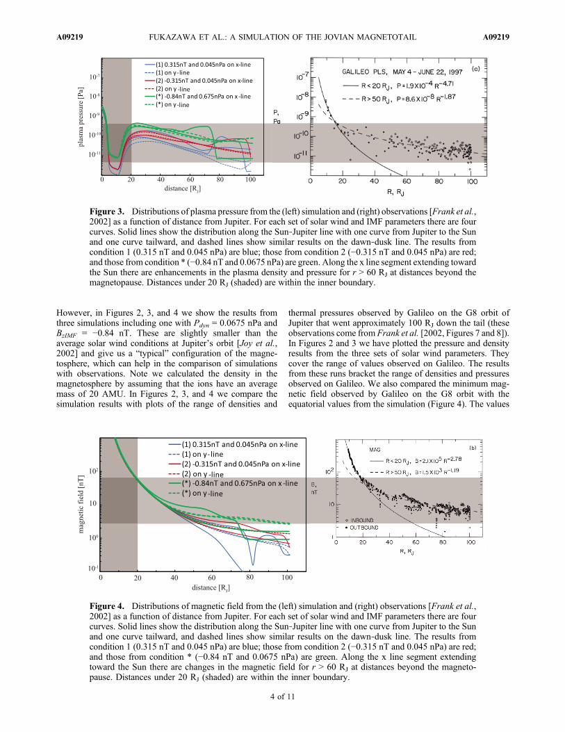
However, in Figures 2, 3, and 4 we show the results fromthree simulations including one with Pdyn = 0.0675 nPa andBzIMF = −0.84 nT. These are slightly smaller than theaverage solar wind conditions at Jupiter’s orbit [Joy et al.,2002] and give us a “typical” configuration of the magne-tosphere, which can help in the comparison of simulationswith observations. Note we calculated the density in themagnetosphere by assuming that the ions have an averagemass of 20 AMU. In Figures 2, 3, and 4 we compare thesimulation results with plots of the range of densities and

thermal pressures observed by Galileo on the G8 orbit ofJupiter that went approximately 100 RJ down the tail (theseobservations come from Frank et al. [2002, Figures 7 and 8]).In Figures 2 and 3 we have plotted the pressure and densityresults from the three sets of solar wind parameters. Theycover the range of values observed on Galileo. The resultsfrom these runs bracket the range of densities and pressuresobserved on Galileo. We also compared the minimum mag-netic field observed by Galileo on the G8 orbit with theequatorial values from the simulation (Figure 4). The values

Figure 4. Distributions of magnetic field from the (left) simulation and (right) observations [Frank et al.,2002] as a function of distance from Jupiter. For each set of solar wind and IMF parameters there are fourcurves. Solid lines show the distribution along the Sun‐Jupiter line with one curve from Jupiter to the Sunand one curve tailward, and dashed lines show similar results on the dawn‐dusk line. The results fromcondition 1 (0.315 nT and 0.045 nPa) are blue; those from condition 2 (−0.315 nT and 0.045 nPa) are red;and those from condition * (−0.84 nT and 0.0675 nPa) are green. Along the x line segment extendingtoward the Sun there are changes in the magnetic field for r > 60 RJ at distances beyond the magneto-pause. Distances under 20 RJ (shaded) are within the inner boundary.

Figure 3. Distributions of plasma pressure from the (left) simulation and (right) observations [Frank et al.,2002] as a function of distance from Jupiter. For each set of solar wind and IMF parameters there are fourcurves. Solid lines show the distribution along the Sun‐Jupiter line with one curve from Jupiter to the Sunand one curve tailward, and dashed lines show similar results on the dawn‐dusk line. The results fromcondition 1 (0.315 nT and 0.045 nPa) are blue; those from condition 2 (−0.315 nT and 0.045 nPa) are red;and those from condition * (−0.84 nT and 0.0675 nPa) are green. Along the x line segment extending towardthe Sun there are enhancements in the plasma density and pressure for r > 60 RJ at distances beyond themagnetopause. Distances under 20 RJ (shaded) are within the inner boundary.


4 of 11

from simulations with the weak solar wind (1 and 2) aresmaller than the observed values for r > 40 RJ. However, thesimulation results of the magnetic field from the near averagepressure runs (*) can cover the observations. These resultsare closer to the observations than the results from the lowdynamic pressure cases. A similar comparison between oursimulation model and observations from Pioneer 10 andGalileo near dawn was presented by Ogino et al. [1998,Figure 2]. Also we show a comparison of B’/(rBr) from asimulation using the average dynamic pressure (0.09 nPa)and northward IMF (0.84 nT) with the model of Khuranaand Schwarzl [2005] to investigate the shape of magneticfield of Jupiter in Figure 5. Figure 5 (left) is the simulationand Figure 5 (right) is Khurana’s model. Figure 5 shows theB’/(rBr) as a color spectrum on the equatorial plane. Thesimulation results are for the average solar wind conditionswhile the model is based on various solar wind conditions.The distribution of simulation results is very similar to themodel around the dawn and dusk sides except close to Jupiteron the dusk side where the simulation shows less bend backthan the model of Khurana and Schwarzl [2005].

3. Simulation Results

[13] Figure 6 shows snapshots of the simulation under thefive different conditions. Figure 6 (top) shows the simula-tion results at t = 165 h under condition 1, and Figure 6(bottom) shows the results at t = 906 h, 1137 h, 1434 h,and 1893 h under conditions 2, 3, 4, and 5, respectively.Figure 6 presents the plasma temperature and flow in theequatorial plane. The plasma temperature is represented as acolor spectrogram with the flow vectors superimposed. Theblack region near Jupiter is inside of the inner magneto-sphere boundary and is not included in the simulation. A setof movies (Movies 1–10) of the Jovian magnetosphere

under all conditions is available.1 There are 10 movies twofor each of the five time periods in Figure 1. Movies 1–5show the magnitude of magnetic field (top) plasma tem-perature and flow vectors (bottom) in the equatorial plane(left) and cross section at Jupiter (right) for condition 1–5.Movies 6–10 show the magnitude of magnetic field (top)plasma temperature and flow vectors (bottom) in the meridianplane (left) and cross section at 1500 RJ (right) for condition1–5. Under condition 1 after the solar wind with dynamicpressure of 0.045 nPa and a northward IMF of 0.315 nTinteracted with Jupiter, a single plasmoid‐like structure wasformed by tail reconnection on closed field lines. Subse-quently it was ejected tailward. This can be seen in Figure 6(top). We subsequently doubled the dynamic pressure butdid not obtain any additional plasmoids. We then turned theIMF southward (condition 2). Now the reconnection was athigh latitudes tailward of the polar cusp. Slowly the mag-netosphere evolved toward a closed magnetosphere. Next,IMF BZ was set to zero, and under these conditions, onlyone plasmoid was ejected, as shown in Figure 6 (panel 2) att = 906 h. This plasmoid was caused by Jovian internalprocesses [Vasyliunas, 1983] since there was no daysidereconnection. Under condition 3, we added oscillations tothe dynamic pressure, which changed the configuration ofthe magnetosphere but did not lead to the ejection ofplasmoid‐like structures (see Figure 6, panel 3). Next we setthe dynamic pressure to 0.023 nPa and then 0.011 nPawithout an IMF. Under these conditions of zero IMF BZ withlow dynamic pressures, we see primarily internal effects. Asingle plasmoid formed but periodic plasmoids were notseen in this set of calculations. We found similar resultsfrom inertial reconnection calculations in our previousshorter tail simulations [Fukazawa et al., 2006]. In addition

Figure 5. Comparison of B’/(rBr) from the simulation with the model of Khurana and Schwarzl[2005] in the equatorial plane. (left) Simulation results for dynamic pressure 0.09 nPa and IMF0.84 nT. (right) From Figure 8 in their paper. Color shows the value of B’/(rBr). The black coloredregion in Figure 5 (left) is within the inner simulation boundary (see section 2).

1Movies 1–10 are available in the HTML.


5 of 11

Figure 6


6 of 11

to these simulations, we ran an extra simulation without IMFand low dynamic pressure lasting 300 h to see any possibleinternal effects. We obtained one plasmoid, but we did notsee periodic plasmoids in the simulation. When we added asmall northward IMF (condition 4) in addition to the lowdynamic pressure we observed periodic plasmoid ejectionsdown the tail at intervals of approximately 55 h. The tailwardvelocity was ∼275 km s−1. These are the conditions underwhich we found periodic plasmoid ejections in the work ofFukazawa et al. [2006]. These results confirm that these solarwind conditions can lead to periodic plasmoid‐like featuresmoving into the distant tail. The plasmoids were found fromx∼ −100 RJ in the tail to the end of the simulation domain atx = −1500 RJ. Figure 6 (panel 4) shows two of thesestructures. Periodic plasmoid ejections also occurred undercondition 5. This will be discussed in section 4.2.[14] Under condition 1, we obtained only one plasmoid.

Under condition 2, high‐latitude reconnection begins toclose the magnetosphere and we found only one plasmoidwhen the southward IMF was increased to zero. Under con-dition 3, no plasmoids were ejected, rather the entire mag-netosphere oscillated. Under condition 4, however, periodicplasmoid ejection occurred. These simulation results sug-gest that the Jovian magnetosphere is significantly affectedby the solar wind and in particular, that the IMF affectsmagnetospheric dynamics.

4. Discussion

4.1. No Periodic Plasmoid Ejections

[15] In the simulation, we find high‐latitude reconnectionwhen the IMF turns southward under condition 3 or duringthe southward intervals when the IMF is rotated. Figure 7shows the plasma temperature and magnetic field vectors

in the noon‐midnight meridian (xz) plane at t = 651 h duringcondition 2. Here the reconnected magnetic field lines athigh latitudes convect tailward. This may correspond to thehigh‐energy structures at high latitudes observed in theJovian magnetotail by New Horizons. Only a single mag-netic island formed at high latitude in the case with constantsouthward IMF. The plasmoid‐like structures observed athigh latitudes by New Horizons may be related to similarstructures formed under a variable IMF.[16] As noted above oscillations in the solar wind

dynamic pressure also can lead to periodic phenomena in themagnetotail. Typical solar wind variations at Jupiter’s orbitcan be inferred from Ulysses observations. Tao et al. [2005]discuss how the solar wind dynamic pressure at Jupiter’sorbit behaves based on an MHD simulation of the solarwind that they compared with Ulysses observations. Theyfound a large number of high dynamic pressure events.In 1998 and 1999 Ulysses observed several pressureenhancements a month when the spacecraft was locatedaround 5 AU. These observations cannot be compareddirectly with Galileo observations at this time since Ulysseswas on the opposite side of the Sun from Jupiter. However,it seems probable that changes in the solar wind pressureanalogous to those in our simulation 3 can occur at Jupiter.However, the changes in the magnetotail resulting fromchanges in the dynamic pressure are not plasmoid‐like.Figure 8 shows the simulation results along the Sun‐Jupiterline for the oscillating solar wind pressure (Figure 8, left)and periodic plasmoid ejections in case 4 (Figure 8, right).In addition to the oscillations in the plasma pressure, themagnetic field (BZ) and plasma velocity (VX and VY) alsoshow periodic changes (see the condition 3 in Movies 3and 8 from 1023 h to 1203 h). The main difference betweenthe plasmoid results and those from the oscillating dynamic

Figure 7. The plasma temperature and magnetic field vectors in the meridian plane for the southwardIMF under condition 3. The temperature per AMU in keV is given by the color spectrogram.

Figure 6. The plasma temperature and flow vectors in the equatorial plane for the simulation at five different instances.The temperature per atomic mass unit (AMU) in keV is given by the color spectrogram. The black region at the center is theinside of the inner boundary of the simulation at 15 RJ.


7 of 11

pressure is that in the case of plasmoid injections, the north‐south component of the magnetic field oscillates from posi-tive to negative. While we cannot rule out pressure variationsbased on the New Horizons observations, the plasmoid likestructures observed on Galileo [Woch et al., 1998; Kruppet al., 1998], have magnetic field changes consistent withplasmoid ejection down the tail [Russell et al., 1998; Vogtet al., 2010]. In our simulations without an IMF there werethree intervals with constant dynamic pressure (Figure 1 andMovies 2, 3, 7, and 8 from 603 h to 723 h and from 1203 h to1323 h). For a dynamic pressure of 0.090 nPa only a singleplasmoid was generated by inertial reconnection. Anotherplasmoid was found when we lowered the pressure (between1203 and 1323 h) with zero IMF. Multiple plasmoids did notform in our calculations with a northward IMF (0.315 nT) andhigh dynamic pressure (0.045 nPa). This is consistent withthe finding of Fukazawa et al. [2006] that multiple plasmaplasmoids required small dynamic pressure.

4.2. Periodic Plasmoid Ejections

[17] The New Horizons spacecraft observed quasiperi-odic variations in the mean plasma energy with periods of3–4 days and velocities of 140–760 km s−1 (H+) at dis-tances from 600 RJ to 2000 RJ down the tail. In addition,these structures were found not only around the equatorialplane but also occasionally at high latitudes [McComas et al.,2007]. One interpretation of the changes in the mean plasmaenergy is that they are plasmoids caused by reconnection

Jupiterward of the spacecraft that are moving tailward[McComas et al., 2007]. In the simulation, periodic plasmoidejection occurred only under conditions 4 and 5 (discussedbelow). The resulting plasmoid‐like structures (periodicity,speed, and location) were similar to those of the observedstructures. In the simulation results, this periodic phenome-non is controlled by the balance between the size of theplasma corotation region and the location of tail reconnec-tion, which in turn are controlled by the northward IMF andsolar wind dynamic pressure [Fukazawa et al., 2006]. Inaddition we demonstrated in our simulation that tailwardmoving enhancements in the plasma temperature also couldarise from pressure pulses in the solar wind.[18] Although the IMF at Jupiter can keep one orientation

for many hours [Walker et al., 2001], it is improbable that itwould remain northward for the entire New Horizons tailpass. In addition at Jupiter, the IMF BY is the dominantcomponent and not IMF BZ. Figure 9 shows a simple pic-ture of magnetic dipole tilt in the yz plane. The dipole fieldrotates with Jupiter and at two instants in time in eachrotation, the direction of the dipole field Bd will be like thatin Figure 9. Then a pure IMF BY (blue arrow) will havecomponents BZ’ and BY’ with respect to the dipole axis.Thus, even a field that is completely in the Y direction willhave a z component with respect to the dipole field (BZ’).As much as 16% of BY is transformed into BZ’ in the simpledipole model in Figure 9. Of course Jupiter’s magneto-spheric magnetic field is not a dipole; however, the dayside

Figure 8. Distribution of magnetic field (BZ), plasma velocity (VX and VY), density, and pressure on theSun‐Jupiter line. (left) From the run with oscillating solar wind dynamic pressure and no IMF. (right)From the simulation with constant dynamic pressure and northward IMF.


8 of 11

magnetic field is compressed by the solar wind and is moredipolar than the middle dayside magnetosphere that isdominated by the equatorial current sheet. The averagevalue of BY is 0.89 nT at Jupiter [Joy et al., 2002]. For thiscase BZ’ can be up to 0.135 nT. This value is almost thesame as that required to obtain periodic plasmoid ejection inour simulation (BZ = 0.105 nT). Thus, intervals duringwhich the magnetic field has a weak BZ component withrespect to the dipole direction should occur frequentlyduring at least part of a 10 h rotation. To investigate theeffects of this projection, we carried out an additionalsimulation in which we reversed IMF BZ every 5 h. Theparameters for this experiment have been plotted in the1620 h to 1980 h interval of Figure 1 and the results of thisnumerical experiment are shown in Figure 6 (bottom) andMovies 5 and 10. Figure 6 (bottom) shows a snapshot withtwo plasmoids in the simulation box. In Movie 10 (top) forthis part of the study the rotation of BZ is shown in the xzplane. Both the noon‐midnight meridian and equatorialplasma temperature panels show the formation of plasmoidlike structures with a much lower frequency than the 10 hperiodicity in the input. Throughout the entire period one ofthese was created approximately every 100 h starting at100 RJ down the tail. These are similar to the New Horizonobservations that have periods of 3–4 days or 4–5 days[McComas et al., 2007; Hill et al., 2009]. The main effectof changing the direction of BZ every 5 h is to increase the

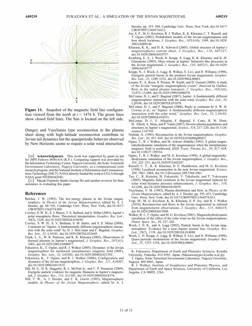
period of plasmoid injection from ∼50 h to ∼100 h. This iscaused by the decrease in the magnetic flux transport.Figure 10 (left) and Figure 10 (right) show time sequencesof magnetic field lines under conditions 4 and 5, respec-tively. Each sequence covers 9 h. Although the configura-tions of magnetic field lines on the dayside seem to bedipolar, these are snapshots in xz plane viewed from theduskside. This obscures the actual configuration of fieldlines near noon. To better demonstrate the configuration wehave plotted a snapshot at t = 1476 h looking from thenorth pole in Figure 11. These magnetic field lines startfrom 80 degrees latitude at Jupiter and are plotted every0.6 h in local time. A similar configuration is also shownby Ogino et al. [1998]. It seems that the field lines arebending around noon so the view of the magnetic field in ameridian plane seems to be dipolar. For constant northwardIMF, magnetic reconnection at the subsolar point occurredand the magnetic flux was continuously convected into thetail. However, in the right hand panels it was intermittent.In Figure 10 subsolar reconnectionwas occurring at 1764 h butnot at t = 1770 and 1773 h because at those times the IMFwas southward and the reconnection had moved to highlatitudes. In our earlier Jupiter simulations the shortest timefor the IMF to influence tail reconnection was approximately30 h (three rotation of Jupiter) [Fukazawa et al., 2006], thusreversing the IMF BZ every 5 h does not change the overallconfiguration of the Jovian magnetosphere but affects thelocal configuration. In particular oscillating the IMF BZ withthe Jovian rotation period decreased the amount of magneticflux accumulated in the tail by factor of 2 and doubled theperiod of plasmoid ejection compared to case 4. Note that thealternating reconnection at high and low latitudes in condition5 is very similar to the model proposed by McComas et al.[2007].

5. Summary

[19] In this paper, we have presented the results from aMHD simulation of the Jovian magnetosphere that describesthe distant tail. We ran five conditions and found thatperiodic plasmoids were ejected for relatively small valuesof northward IMF and dynamic pressure. They alsooccurred when we changed the direction of a small IMFwith a 10 h period. For this case we found evidence thatplasma sheet reconnection driven by short intervals ofnorthward IMF can contribute quasiperiodic plasmoid‐likestructures to the distant tail. The simulation results aresimilar to the New Horizons observations. In our earlierstudy we found that periodic plasmoids were launchedwhen the dynamic pressure and IMF were small enough thatreconnected flux tubes could convect all of the way aroundthe magnetosphere and reconnect again. Since we only needa small component of the IMF along the dipole direction theperiodic ejection of plasmoids down the tail can occur evenif the IMF is not maintained northward. The plasmoidejections are controlled by the solar wind dynamic pressureprovided there is some reconnection. When the IMF has asouthward component reconnection occurs in the tail lobesand magnetic islands are formed however they are notperiodic. For this condition plasmoid‐like structures canoccur at high latitudes. Finally when we turned off the IMFwe found evidence for inertial reconnection. Thus, both

Figure 9. Schematic diagram of the magnetic dipole tiltand IMF in the yz plane. Bd is the dipole magnetic fieldand the blue BY arrow shows a pure IMF BY. Here �tilt repre-sents the angle of magnetic dipole tilt to the rotation of Jupi-ter. BY’ and BZ’ represent projections of BY.


9 of 11

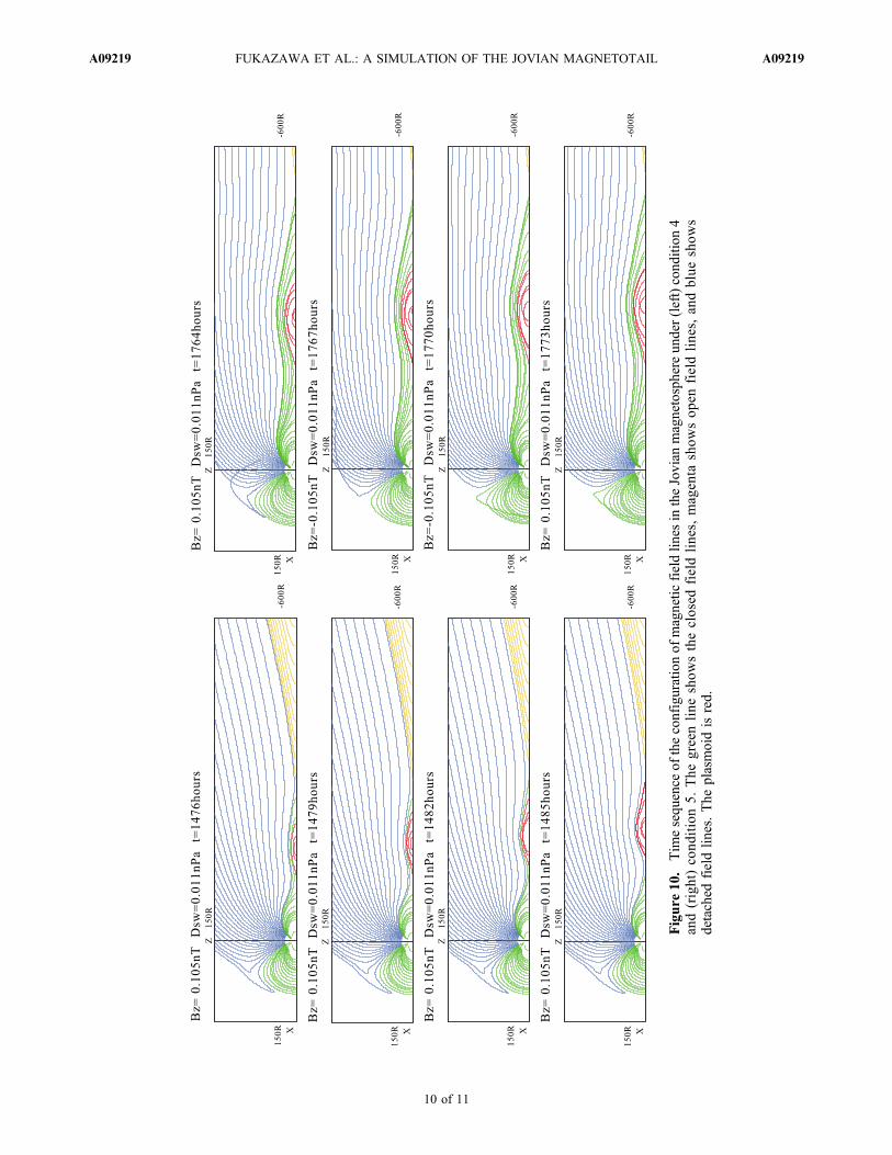
Figure

10.

Tim

esequence

oftheconfigurationof

magnetic

fieldlin

esin

theJovian

magnetosphere

under(left)condition

4and(right)cond

ition5.

The

greenline

show

stheclosed

fieldlines,

magenta

show

sop

enfieldlines,

andblue

show

sdetached

fieldlin

es.The

plasmoidisred.


10 of 11

Dungey and Vasyliunas type reconnection in the plasmasheet along with high‐latitude reconnection contribute toJovian tail dynamics but the quasiperiodic behavior observedby New Horizons seems to require a solar wind interaction.

[20] Acknowledgments. This work was supported by grant‐in‐aidfor JSPS Fellows 09J01416 (K.F.). Computing support was provided bythe Information TechnologyCenter, NagoyaUniversity, the Solar‐TerrestrialEnvironment Laboratory, Nagoya University, as a computational jointresearch program, and the National Institute of Information and Communica-tions Technology (NICT). NASA directly funded the work at UCLA throughNASA grant NNX08AQ54G.[21] Masaki Fujimoto thanks George Ho and another reviewer for their

assistance in evaluating this paper.

ReferencesBelcher, J. W. (1983), The low‐energy plasma in the Jovian magne-tosphere, in Physics of the Jovian Magnetosphere, edited by A. J.Dessler, pp. 68–105, Cambridge Univ. Press, New York, doi:10.1017/CBO9780511564574.005.

Cowley, S. W. H., E. J. Bunce, T. S. Stallard, and S. Miller (2003), Jupiter’spolar ionospheric flows: Theoretical interpretation, Geophys. Res. Lett.,30(5), 1220, doi:10.1029/2002GL016030.

Cowley, S. W. H., S. V. Badman, S. M. Imber, and S. E. Milan (2008),Comment on “Jupiter: A fundamentally different magnetospheric interac-tion with the solar wind” by D. J. McComas and F. Bagenal, Geophys.Res. Lett., 35, L10101, doi:10.1029/2007GL032645.

Frank, L. A., W. R. Paterson, and K. K. Khurana (2002), Observations ofthermal plasmas in Jupiter’s magnetotail, J. Geophys. Res., 107(A1),1003, doi:10.1029/2001JA000077.

Fukazawa, K., T. Ogino, and R. J. Walker (2005), Dynamics of the Jovianmagnetosphere for northward interplanetary magnetic field (IMF),Geophys. Res. Lett., 32, L03202, doi:10.1029/2004GL021392.

Fukazawa, K., T. Ogino, and R. J. Walker (2006), Configuration anddynamics of the Jovian magnetosphere, J. Geophys. Res., 111, A10207,doi:10.1029/2006JA011874.

Hill, M. E., D. K. Haggerty, R. L. McNutt Jr., and C. P. Paranicas (2009),Energetic particle evidence for magnetic filaments in Jupiter’s magneto-tail, J. Geophys. Res., 114, A11201, doi:10.1029/2009JA014374.

Hill, T. W., A. J. Dessler, and C. K. Goertz (1983), Magnetosphericmodels, in Physics of the Jovian Magnetosphere, edited by A. J.

Dessler, pp. 353–394, Cambridge Univ. Press, New York, doi:10.1017/CBO9780511564574.012.

Joy, S. P., M. G. Kivelson, R. J. Walker, K. K. Khurana, C. T. Russell, andT. Ogino (2002), Probabilistic models of the Jovian magnetopause andbow shock locations, J. Geophys. Res., 107(A10), 1309, doi:10.1029/2001JA009146.

Khurana, K. K., and H. K. Schwarzl (2005), Global structure of Jupiter’smagnetospheric current sheet, J. Geophys. Res., 110, A07227,doi:10.1029/2004JA010757.

Kronberg, E. A., J. Woch, N. Krupp, A. Lagg, K. K. Khurana, and K.‐H.Glassmeier (2005), Mass release at Jupiter: Substorm‐like processes inthe Jovian magnetotail, J. Geophys. Res., 110, A03211, doi:10.1029/2004JA010777.

Krupp, N., J. Woch, A. Lagg, B. Wilken, S. Livi, and D. Williams (1998),Energetic particle bursts in the predawn Jovian magnetotail, Geophys.Res. Lett., 25, 1249–1252, doi:10.1029/98GL00863.

Louarn, P., A. Roux, S. Perraut, W. Kurth, and D. Gurnett (2000), A studyof the Jovian “energetic magnetospheric events” observed by Galileo:Role in the radial plasma transport, J. Geophys. Res., 105(A6),13,073–13,088, doi:10.1029/1999JA900478.

McComas, D. J., and F. Bagenal (2007), Jupiter: A fundamentally differentmagnetospheric interaction with the solar wind, Geophys. Res. Lett., 34,L20106, doi:10.1029/2007GL031078.

McComas, D. J., and F. Bagenal (2008), Reply to comment by S. W. H.Cowley et al., on “Jupiter: A fundamentally different magnetosphericinteraction with the solar wind,” Geophys. Res. Lett., 35, L10103,doi:10.1029/2008GL034351.

McComas, D. J., F. Allegrini, F. Bagenal, F. Crary, R. W. Ebert,H. Elliott, A. Stern, and P. Valek (2007), Diverse plasma populations andstructures in Jupiter’s magnetotail, Science, 318, 217–220, doi:10.1126/science.1147393.

Nishida, A. (1983), Reconnection in the Jovian magnetosphere, Geophys.Res. Lett., 10, 451–454, doi:10.1029/GL010i006p00451.

Ogino, T., R. J. Walker, and M. Ashour‐Abdalla (1992), A global magne-tohydrodynamic simulation of the magnetopause when the interplanetarymagnetic field is northward, IEEE Trans. Plasma Sci., 20, 817–828,doi:10.1109/27.199534.

Ogino, T., R. J. Walker, and M. G. Kivelson (1998), A global magnetohy-drodynamic simulation of the Jovian magnetosphere, J. Geophys. Res.,103, 225–235, doi:10.1029/97JA02247.

Russell, C. T., K. K. Khurana, D. E. Huddleston, and M. G. Kivelson(1998), Localized reconnection in the near Jovian magnetotail, Science,280, 1061–1064, doi:10.1126/science.280.5366.1061.

Tao, C., R. Kataoka, H. Fukunishi, Y. Takahashi, and T. Yokoyama(2005), Magnetic field variations in the Jovian magnetotail induced bysolar wind dynamic pressure enhancements, J. Geophys. Res., 110,A11208, doi:10.1029/2004JA010959.

Vasyliunas, V. M. (1983), Plasma distribution and flow, in Physics of theJovian Magnetosphere, edited by A. J. Dessler, pp. 395–453, CambridgeUniv. Press, New York, doi:10.1017/CBO9780511564574.013.

Vogt, M., M. G. Kivelson, K. K. Khurana, S. P. Joy, and R. J. Walker(2010), Reconnection and flows in the Jovian magnetotail as inferredfrom magnetometer observations, J. Geophys. Res., 115, A06219,doi:10.1029/2009JA015098.

Walker, R. J., T. Ogino, and M. G. Kivelson (2001), Magnetohydrodynamicsimulation of the effect of the solar wind on the Jovian magnetosphere,Planet. Space. Sci., 49, 237–245.

Woch, J. N. K., and A. Lagg (2002), Particle bursts in the Jovian mag-netosphere: Evidence for a near‐Jupiter neutral line, Geophys. Res.Lett., 29(7), 1138, doi:10.1029/2001GL014080.

Woch, J., N. Krupp, A. Lagg, B. Wilken, S. Livi, and D. Williams (1998),Quasi‐periodic modulations of the Jovian magnetotail, Geophys. Res.Lett., 25, 1253–1256, doi:10.1029/98GL00861.

K. Fukazawa, Department of Earth and Planetary Sciences, KyushuUniversity, Fukuoka, 812‐8581, Japan. ([email protected]‐u.ac.jp)T. Ogino, Solar‐Terrestrial Environment Laboratory, Nagoya University,

Nagoya, 464‐8601, Japan.R. J. Walker, Institute of Geophysics and Planetary Physics, and

Department of Earth and Space Sciences, University of California, LosAngeles, CA 90095, USA.

Figure 11. Snapshot of the magnetic field line configura-tion viewed from the north at t = 1476 h. The green linesshow closed field lines. The Sun is located on the left side.


11 of 11

a simulation study of dynamics in the distant jovian magnetotail · · 2011-08-24a simulation...

Documents