a smart material for the in situ detection of mercury in fish · a smart material for the in situ...
TRANSCRIPT
S1
Supporting Information
A smart material for the in situ detection of mercury in fishJosé García-Calvo, Saúl Vallejos, Félix C. García, Josefa Rojo, José M. García,* and Tomás Torroba*Department of Chemistry, Faculty of Science, University of Burgos, 09001 Burgos, Spain.
Materials and methods S2
Synthesis of starting materials S3-S10
Preparation of the functional polymers S11-S15
Qualitative tests S16-S19
Quantitative tests S20-S32
Analysis of fish samples S33-S38
Electronic Supplementary Material (ESI) for ChemComm.This journal is © The Royal Society of Chemistry 2016

S2
Experimental Part:
Materials and methods: The reactions performed with air sensitive reagents were conducted under dry nitrogen. The solvents were previously distilled under nitrogen over calcium hydride or sodium filaments. Melting points were determined in a Gallenkamp apparatus and are not corrected. FT-IR spectra were recorded on potassium bromide pellet with a JASCO FT/IR-4200. NMR spectra were recorded in Varian Mercury-300 and Varian Unity Inova-400 machines, in DMSO-d6, CDCl3, CD3CN, CD3OD. Chemical shifts are reported in ppm with respect to residual solvent protons, coupling constants (JX-X’) are reported in Hz. Elemental analyses of C, H and N were taken in a Leco CHNS-932. EI mass spectra were taken in a Micromass AutoSpec machine, by electronic impact at 70 eV. MALDI-TOF mass spectra were measured on a MALDI-TOF Bruker Autoflex Mass Spectrometry instrument using DCTB and DIT matrixes. Quantitative UV-visible measures were performed with a Hitachi U-3900, in 1 cm UV cells at 25ºC. Fluorescence spectra were recorded in a Varian Cary Eclipse or a Hitachi F-7000 FL spectrofluorometers, in 1 cm quarz cells at 25ºC. The pH values were measured at room temperature using a Metrohm 16 DMS Titrino pH meter fitted out with a combined glass electrode and a 3 M KCl solution as a liquid junction, which was calibrated with Radiometer Analytical SAS buffer solutions.
S3
SYNTHESIS:
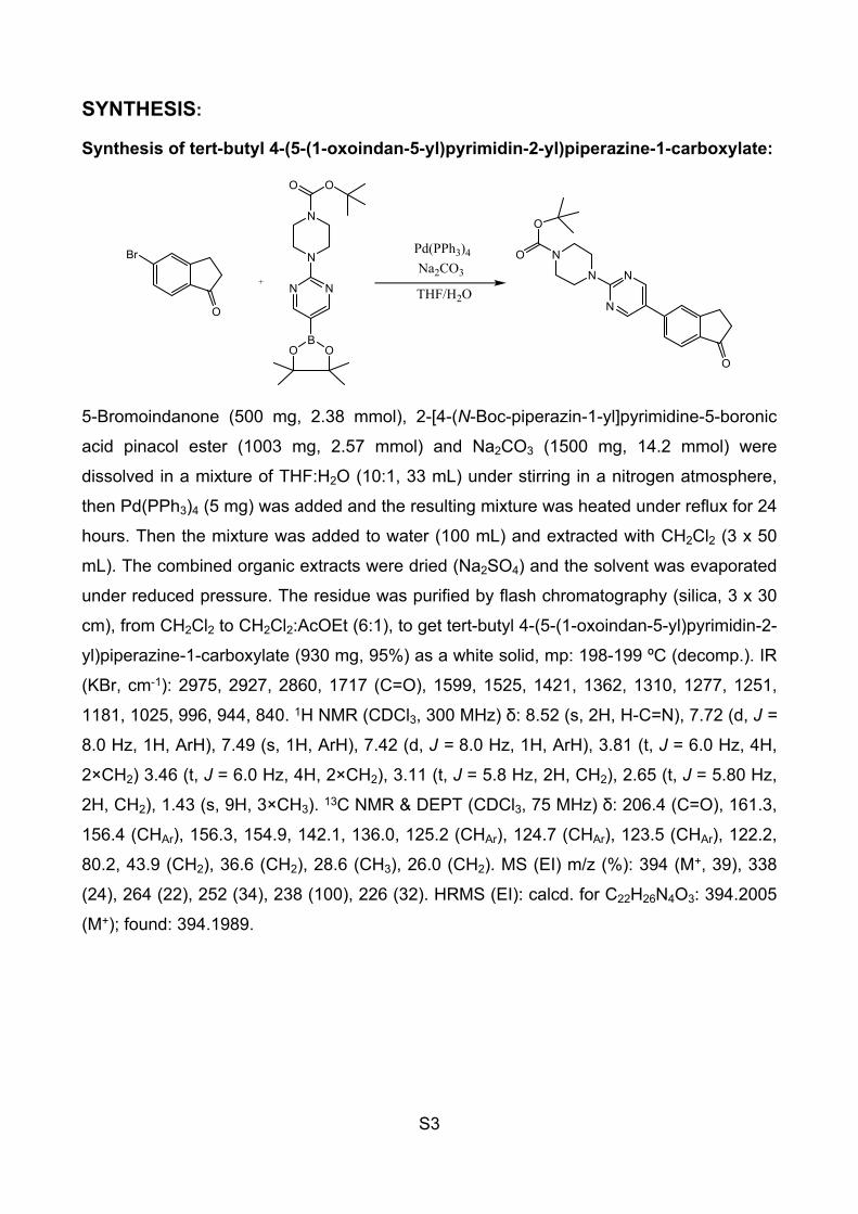
Synthesis of tert-butyl 4-(5-(1-oxoindan-5-yl)pyrimidin-2-yl)piperazine-1-carboxylate:
O
O
Br
+N N
N
BOO
N
O O
N
N
N
NO
O
THF/H2O
Pd(PPh3)4Na2CO3
5-Bromoindanone (500 mg, 2.38 mmol), 2-[4-(N-Boc-piperazin-1-yl]pyrimidine-5-boronic
acid pinacol ester (1003 mg, 2.57 mmol) and Na2CO3 (1500 mg, 14.2 mmol) were
dissolved in a mixture of THF:H2O (10:1, 33 mL) under stirring in a nitrogen atmosphere,
then Pd(PPh3)4 (5 mg) was added and the resulting mixture was heated under reflux for 24
hours. Then the mixture was added to water (100 mL) and extracted with CH2Cl2 (3 x 50
mL). The combined organic extracts were dried (Na2SO4) and the solvent was evaporated
under reduced pressure. The residue was purified by flash chromatography (silica, 3 x 30
cm), from CH2Cl2 to CH2Cl2:AcOEt (6:1), to get tert-butyl 4-(5-(1-oxoindan-5-yl)pyrimidin-2-
yl)piperazine-1-carboxylate (930 mg, 95%) as a white solid, mp: 198-199 ºC (decomp.). IR
(KBr, cm-1): 2975, 2927, 2860, 1717 (C=O), 1599, 1525, 1421, 1362, 1310, 1277, 1251,
1181, 1025, 996, 944, 840. 1H NMR (CDCl3, 300 MHz) δ: 8.52 (s, 2H, H-C=N), 7.72 (d, J =
8.0 Hz, 1H, ArH), 7.49 (s, 1H, ArH), 7.42 (d, J = 8.0 Hz, 1H, ArH), 3.81 (t, J = 6.0 Hz, 4H,
2×CH2) 3.46 (t, J = 6.0 Hz, 4H, 2×CH2), 3.11 (t, J = 5.8 Hz, 2H, CH2), 2.65 (t, J = 5.80 Hz,
2H, CH2), 1.43 (s, 9H, 3×CH3). 13C NMR & DEPT (CDCl3, 75 MHz) δ: 206.4 (C=O), 161.3,
156.4 (CHAr), 156.3, 154.9, 142.1, 136.0, 125.2 (CHAr), 124.7 (CHAr), 123.5 (CHAr), 122.2,
80.2, 43.9 (CH2), 36.6 (CH2), 28.6 (CH3), 26.0 (CH2). MS (EI) m/z (%): 394 (M+, 39), 338
(24), 264 (22), 252 (34), 238 (100), 226 (32). HRMS (EI): calcd. for C22H26N4O3: 394.2005
(M+); found: 394.1989.

S4
1.52.02.53.03.54.07.58.08.5f1 (ppm)
9.72
2.00
2.00
4.30
4.25
1.20
1.08
0.96
1.90
1.43
2.63
2.65
2.67
3.09
3.11
3.13
3.45
3.46
3.48
3.80
3.81
3.83
7.26
7.39
7.42
7.49
7.71
7.73
8.52
Figure S1: 1H NMR (CDCl3, 300 MHz) of tert-butyl 4-(5-(1-oxoindan-5-yl)pyrimidin-2-yl)piperazine-1-carboxylate
30405060708090100110120130140150160170180190200210f1 (ppm)
26.0
028
.55
36.5
5
43.8
6
77.1
680
.22
122.
1812
3.47
124.
6712
5.19
136.
01
142.
06
154.
9115
6.29
156.
3516
1.25
206.
39
Figure S2: 13C NMR (CDCl3, 75 MHz) of tert-butyl 4-(5-(1-oxoindan-5-yl)pyrimidin-2-yl)piperazine-1-carboxylate
S5
30405060708090100110120130140150160f1 (ppm)
26.0
028
.55
36.5
5
43.8
6
123.
4712
4.66
125.
18
156.
35
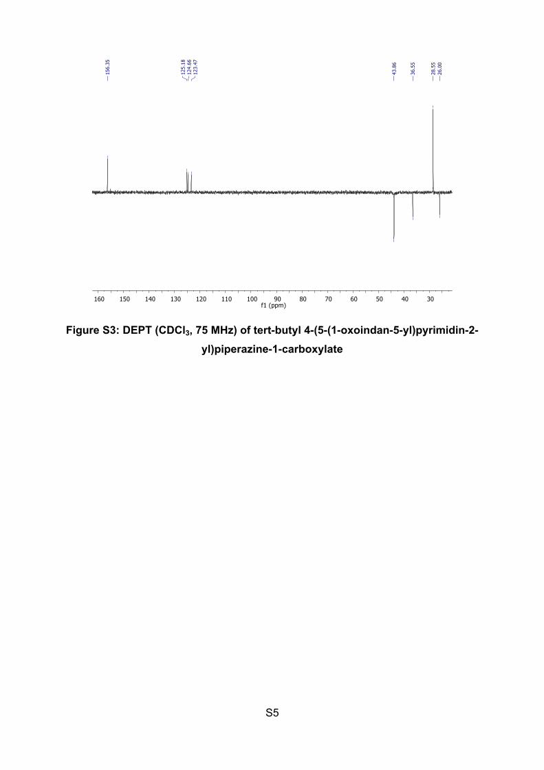
Figure S3: DEPT (CDCl3, 75 MHz) of tert-butyl 4-(5-(1-oxoindan-5-yl)pyrimidin-2-yl)piperazine-1-carboxylate

S6
Synthesis of 5-(2-(piperazin-1-yl)pyrimidin-5-yl)indan-1-one:
O
N
N
N
NO
O
O
N
N
N
HN
CF3COOH
CH2Cl2
1a
Trifluoroacetic acid (10 mL, ρ= 1.489 g/mL, 130.59 mmol) was added dropwise with
stirring to a solution of tert-butyl 4-(5-(1-oxoindan-5-yl)pyrimidin-2-yl)piperazine-1-
carboxylate (874 mg, 2.22 mmol) in CH2Cl2 (20 mL) and the resulting mixture was stirred
at room temperature for 15 minutes. Then the mixture was added to water (50 mL),
basified to pH= 10 with 5% NaOH and extracted with CH2Cl2 (4 x 50 mL). The combined
organic extracts were dried (Na2SO4), the solvent was evaporated under reduced pressure
and the residue was recrystallized from CH2Cl2-MeOH (5:1) to get 5-(2-(piperazin-1-
yl)pyrimidin-5-yl)indan -1-one (617 mg, 95%) as a white solid, mp: 189-190 ºC (decomp.).
IR (KBr, cm-1): 3221 (N-H), 2940, 2843, 1706 (C=O), 1603, 1502, 1455, 1363, 1307, 1260,
1117, 940. 1H NMR (CDCl3, 300 MHz) δ: 8.55 (s, 2H, H-C=N), 7.76 (d, J = 8.0 Hz, 1H,
ArH), 7.52 (s, 1H, ArH), 7.44 (d, J = 8.0 Hz, 1H, ArH), 3.84 (d, J = 6.0 Hz, 4H, 2×CH2),
3.15 (d, J = 6.0 Hz, 2H, CH2), 2.92 (d, J = 6.0 Hz, 4H, 2×CH2), 2.69 (d, J = 6.0 Hz, 2H,
CH2), 1.84 (s, 1H, NH). 13C NMR & DEPT (CDCl3, 75 MHz) δ: 206.3 (C=O), 161.3, 156.2
(CHAr), 156.2, 142.2, 135.8, 125.0 (CHAr), 124.5 (CHAr), 123.2 (CHAr), 121.5, 46.1 (CH2),
45.1 (CH2), 36.5 (CH2), 25.9 (CH2). MS (EI) m/z (%): 294 (M+, 22), 252 (100), 238 (29),
226 (59). HRMS (EI): calcd. for C17H18N4O: 294.1481 (M+); found: 294.1482.

S7
2.02.53.03.54.04.55.05.56.06.57.07.58.08.5f1 (ppm)
2.19
4.53
2.21
4.57
1.29
1.09
1.00
2.00
1.84
2.67
2.69
2.71
2.91
2.92
2.94
3.13
3.15
3.17
3.82
3.84
3.85
7.26
7.43
7.46
7.52
7.75
7.78
8.56
8.56
Figure S4: 1H NMR (CDCl3, 300 MHz) of 5-(2-(piperazin-1-yl)pyrimidin-5-yl)indan-1-one
30405060708090100110120130140150160170180190200210f1 (ppm)
25.9
3
36.4
8
45.1
146
.06
77.1
6
121.
5412
3.24
124.
5412
4.99
135.
80
142.
15
156.
21
161.
26
206.
33
Figure S5: 13C NMR (CDCl3, 75 MHz) of 5-(2-(piperazin-1-yl)pyrimidin-5-yl)indan-1-one
S8
30405060708090100110120130140150f1 (ppm)
25.9
3
36.4
8
45.1
146
.06
123.
2312
4.54
124.
99
156.
21
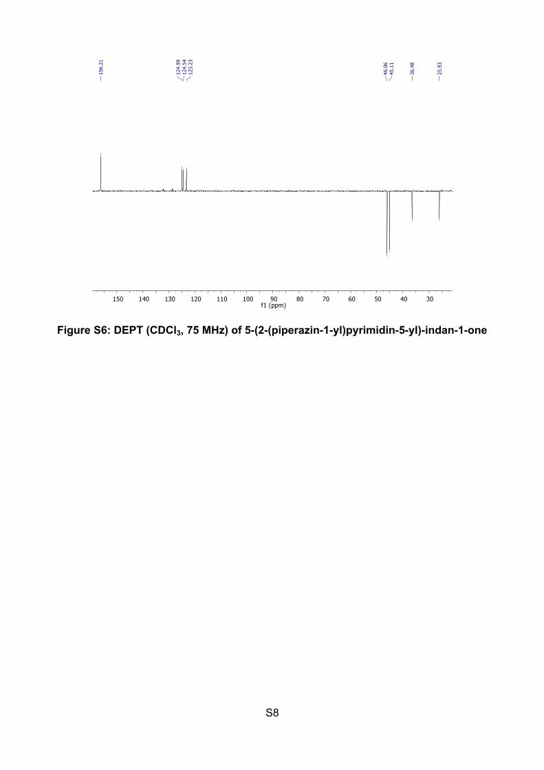
Figure S6: DEPT (CDCl3, 75 MHz) of 5-(2-(piperazin-1-yl)pyrimidin-5-yl)-indan-1-one

S9
Synthesis of N-(4-azidophenyl)-4-(5-(1-oxo-indan-5-yl)pyrimidin-2-yl)piperazin-1-carbothioamide JG10:
NHN
N
N
O
NN
N
N
O
NH
SNNN
N
N
C SNNCHCl3+
A 50 ml Schlenk, with a magnetic stirrer, was charged with 50 mg of 5-[4-(piperazine-1-yl)pyrimidin]indanone (0.17 mmol) and 20 ml of CHCl3. The resulting solution stirred under nitrogen in an ice bath for five minutes and then 40.66 mg of 1-azide-4-isothiocyanatebenzene (0.23 mmol) were added to the solution. The solution was stirred for 20 minutes at 0 ºC, then for 21 hours at room temperature and then refluxed for 30 minutes at 35 oC. The presence of the initial reagents was followed by thin layer chromatography. TLC was eluted with dichloromethane:methanol (50:1). The solvent was evaporated and the product was purified under flash column chromatography from dichloromethane to dichloromethane:methanol 50:1 v/v to obtain 55.4 mg of N-(4-azidophenyl)-4-(5-(1-oxoindan-5-yl)pyrimidin-2-yl)piperazin-1-carbothioamide (56% yield) as a white solid, mp: 188-190 oC (decomp.). IR (KBr, cm-1): 3359 (N-H), 3022, 2921, 2851, 2110 (N-=N+=N-), 1697 (C=O), 1597, 1503, 1453, 1420, 1355, 1307, 1259, 1224. 1H NMR (DMSO-d6, 400 MHz) δ: 9.43 (s, 1H, N-H), 8.86 (s, 2H, H-C=N), 7.89 (s, ArH), 7.73 (d, J = 8.7 Hz, 1H, ArH), 7.68 (d, J = 8.1 Hz, 1H, ArH), 7.36 (d, J = 8.7 Hz, 2H, ArH), 7.06 (d, J = 8.7 Hz, 2H, ArH), 4.06 (m, 4H, 2×CH2) 3.93 (m, 4H, 2×CH2), 3.14 (t, J =5.8 Hz, 2H, CH2), 2.66 (t, J = 5.8 Hz, 2H, CH2). 13C NMR (DMSO-d6, 100 MHz) δ: 205.9 (C=O), 181.4 (C=S), 160.5, 156.4 (2×CHAr), 156.2, 141.1, 138.1, 135.3, 135.2, 127.0 (2×CHAr), 124.7 (CHAr), 123.6 (CHAr), 123.3 (CHAr), 121.2, 118.7 (2×CHAr), 47.5 (CH2), 43.0 (CH2), 36.1 (CH2), 25.5 (CH2). MS (MALDI) m/z (%): 471 (M++1, 21), 443 (100), 411 (45), 393 (19), 337 (95), 295 (43). HRMS (MALDI): calcd. for C24H23N8OS: 471.1710 (M++1); found: 471.1803 (M++1).

S10
2.53.03.54.04.55.05.56.06.57.07.58.08.59.09.5f1 (ppm)
2.39
2.18
8.00
1.89
1.90
2.05
1.00
1.96
0.93
2.65
2.66
2.66
2.67
2.67
2.68
3.13
3.15
3.16
3.92
3.93
3.94
3.95
4.04
4.05
4.06
4.07
7.06
7.06
7.07
7.08
7.36
7.36
7.37
7.38
7.68
7.70
7.73
7.75
7.89
8.87
8.87
9.43
Figure S7: 1H NMR (CDCl3, 300 MHz) of N-(4-azidophenyl)-4-(5-(1-oxo-indan-5-yl)pyrimidin-2-yl)piperazin-1-carbothioamide JG10
2030405060708090100110120130140150160170180190200210f1 (ppm)
25.5
3
36.1
1
42.9
8
47.4
6
109.
31
118.
6612
1.21
123.
3112
3.59
124.
6712
7.00
135.
2213
5.32
138.
1314
1.11
156.
2315
6.38
160.
53
181.
44
205.
59
Figure S8: 13C NMR (CDCl3, 75 MHz) of N-(4-azidophenyl)-4-(5-(1-oxo-indan-5-yl)pyrimidin-2-yl)piperazin-1-carbothioamide JG10
S11
Preparation of the functional polymers
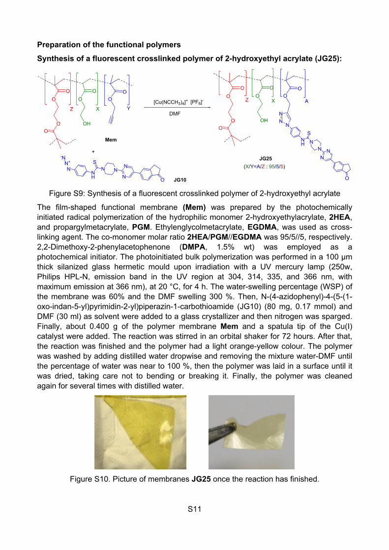
Synthesis of a fluorescent crosslinked polymer of 2-hydroxyethyl acrylate (JG25):
NNN
N
ONH
SN
N+-N
DMF
OO
O
OO
OH
OO
O
OO
O
OO
OH
OO
O
NN
NN
O
NH
SN
NN
+JG25
Mem
JG10
Z X
Z X A
(X/Y=A/Z : 95/5/5)
Y[Cu(NCCH3)4]+ [PF6]-
Figure S9: Synthesis of a fluorescent crosslinked polymer of 2-hydroxyethyl acrylate
The film-shaped functional membrane (Mem) was prepared by the photochemically initiated radical polymerization of the hydrophilic monomer 2-hydroxyethylacrylate, 2HEA, and propargylmetacrylate, PGM. Ethylenglycolmetacrylate, EGDMA, was used as cross-linking agent. The co-monomer molar ratio 2HEA/PGM//EGDMA was 95/5//5, respectively. 2,2-Dimethoxy-2-phenylacetophenone (DMPA, 1.5% wt) was employed as a photochemical initiator. The photoinitiated bulk polymerization was performed in a 100 μm thick silanized glass hermetic mould upon irradiation with a UV mercury lamp (250w, Philips HPL-N, emission band in the UV region at 304, 314, 335, and 366 nm, with maximum emission at 366 nm), at 20 °C, for 4 h. The water-swelling percentage (WSP) of the membrane was 60% and the DMF swelling 300 %. Then, N-(4-azidophenyl)-4-(5-(1-oxo-indan-5-yl)pyrimidin-2-yl)piperazin-1-carbothioamide (JG10) (80 mg, 0.17 mmol) and DMF (30 ml) as solvent were added to a glass crystallizer and then nitrogen was sparged. Finally, about 0.400 g of the polymer membrane Mem and a spatula tip of the Cu(I) catalyst were added. The reaction was stirred in an orbital shaker for 72 hours. After that, the reaction was finished and the polymer had a light orange-yellow colour. The polymer was washed by adding distilled water dropwise and removing the mixture water-DMF until the percentage of water was near to 100 %, then the polymer was laid in a surface until it was dried, taking care not to bending or breaking it. Finally, the polymer was cleaned again for several times with distilled water.
Figure S10. Picture of membranes JG25 once the reaction has finished.

S12
Characterization: The characterization was carried out by SEM analysis, with gold and carbon recap. The atomic proportion was indicated by X-ray analysis on different areas of the polymer. The proportion between oxygen or carbon and sulfur atoms was very similar to the theoretical results associated to a 100 % stoichiometric reaction (60-100 % depending on the area).
Coating %Sreal/%Steor
Gold 79,4
Gold 100,7
Gold 83,5
Carbon 84,9
Carbon 68,5
Carbon 93,7
Figure S11. [A] SEM image of JG25 [B] X-ray fluorescence analysis from JG25.
Figure S12. IR (ATR, cm-1): 3529-3356 (O-H), 2968-2859 (C-H), 1708 (C=O), 1514 (Car-Car), 1441, 1393, 1264, 1167, 1077, 1043, 893, 839 (fingerprint zone).
[A]
[B]
S13
The signal at 1514 and 1598 (very low) cm-1 are the only signals associated to the presence of the probe, because there is no presence of these signals on the initial IR spectrum, and their intensity has to be very low due to the low percentage (5%) (Inset in the Figure S12).
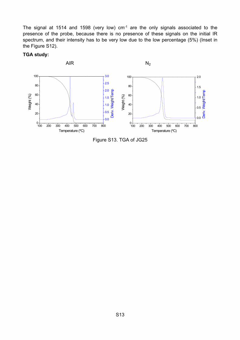
TGA study:
AIR N2
100 200 300 400 500 600 700 8000
20
40
60
80
100
Temperature (ºC)
Wei
ght (
%)
0.0
0.5
1.0
1.5
2.0
2.5
3.0
Deriv
. Wei
ght/T
emp
100 200 300 400 500 600 700 8000
20
40
60
80
100
Temperature (ºC)
Wei
ght (
%)
0.0
0.5
1.0
1.5
2.0
Deriv
. Wei
ght/T
emp
Figure S13. TGA of JG25
S14
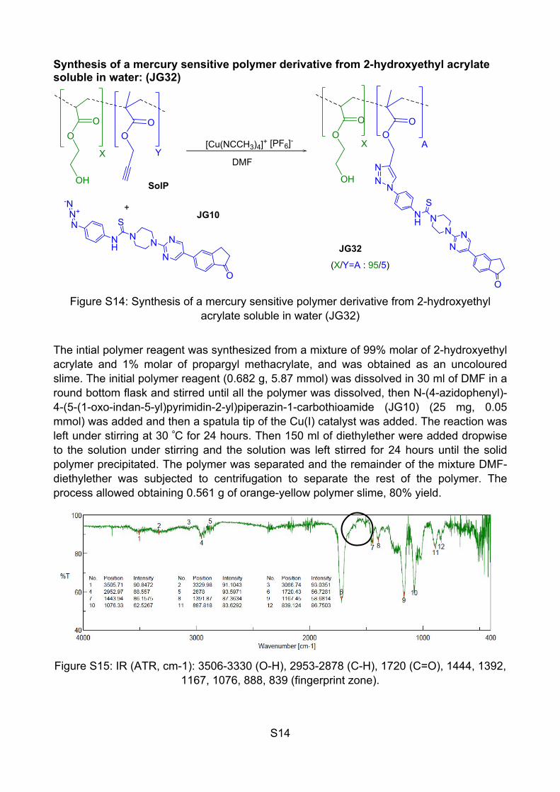
Synthesis of a mercury sensitive polymer derivative from 2-hydroxyethyl acrylate soluble in water: (JG32)
NN
N
N
O
NH
SNN+
-N
DMF
OO
OH
OO
OO
OH
OO
NN
NN
O
NH
SN
NN
+
JG32
SolP
JG10
XX A
(X/Y=A : 95/5)
Y[Cu(NCCH3)4]+ [PF6]-
Figure S14: Synthesis of a mercury sensitive polymer derivative from 2-hydroxyethyl acrylate soluble in water (JG32)
The intial polymer reagent was synthesized from a mixture of 99% molar of 2-hydroxyethyl acrylate and 1% molar of propargyl methacrylate, and was obtained as an uncoloured slime. The initial polymer reagent (0.682 g, 5.87 mmol) was dissolved in 30 ml of DMF in a round bottom flask and stirred until all the polymer was dissolved, then N-(4-azidophenyl)-4-(5-(1-oxo-indan-5-yl)pyrimidin-2-yl)piperazin-1-carbothioamide (JG10) (25 mg, 0.05 mmol) was added and then a spatula tip of the Cu(I) catalyst was added. The reaction was left under stirring at 30 ºC for 24 hours. Then 150 ml of diethylether were added dropwise to the solution under stirring and the solution was left stirred for 24 hours until the solid polymer precipitated. The polymer was separated and the remainder of the mixture DMF-diethylether was subjected to centrifugation to separate the rest of the polymer. The process allowed obtaining 0.561 g of orange-yellow polymer slime, 80% yield.
Figure S15: IR (ATR, cm-1): 3506-3330 (O-H), 2953-2878 (C-H), 1720 (C=O), 1444, 1392, 1167, 1076, 888, 839 (fingerprint zone).

S15
In this compound, the signals at 1600-1500 cm-1 can be barely distinguished from the noise. It should be because, for this polymer, the percentage of the fluorogenic probe is too low (1%) which agrees with the previous results.
S16
QUALITATIVE TESTS
General conditions:
The fluorescence tests were done with some cations and anions. The solutions of the probe were tested by increasing the concentration of cations and anions in solution and checking the variation in colour and/or fluorescence under visible and UV light (366 nm).
The cations and anions solutions were prepared in deionized water and the counterions were selected as non-coordinant counterions; tetrabutylamonium for anions and perchlorate or triflate for cations, except Au3+ which is a HAuCl4 solution in water.
The results of these tests are shown when there is a change that can be appreciated, the anions tests aren’t usually shown because there is no change in presence of anions.
Tests with JG10, azide probe:
In order to check the fluorescence of the azide probe before reaction with the polymer, a qualitative test was done from 10-5 M solutions in MeOH:H2O 60:40, due to its low solubility in water.
Figure S16. Fluorescence in the presence of cations excess after 24 hours
The fluorescence increases very little in presence of Ag+ and increases strongly in the presence of Hg2+ and Au3+.
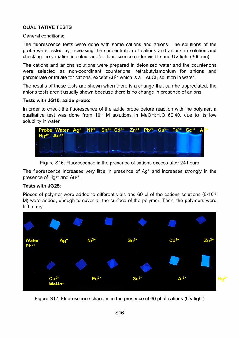
Tests with JG25:
Pieces of polymer were added to different vials and 60 µl of the cations solutions (5·10-3 M) were added, enough to cover all the surface of the polymer. Then, the polymers were left to dry.
Figure S17. Fluorescence changes in the presence of 60 µl of cations (UV light)
Water Ag+ Ni2+ Sn2+ Cd2+ Zn2+ Pb2+
Cu2+ Fe3+ Sc3+ Al3+ Hg2+ MeHg+
Probe Water Ag+ Ni2+ Sn2+ Cd2+ Zn2+ Pb2+ Cu2+ Fe3+ Sc3+ Al3+ Hg2+ Au3+
S17
Ag+
Ni2+
Sn2+
Cd2+
Zn2+
Pb2+
Cu2+
Fe3+
Sc3+
Al3+
Hg2+
MeHg+
0,0 0,5 1,0 1,5 2,0 2,5 3,0 3,5
Final emission/Initial emission
Cat
ion
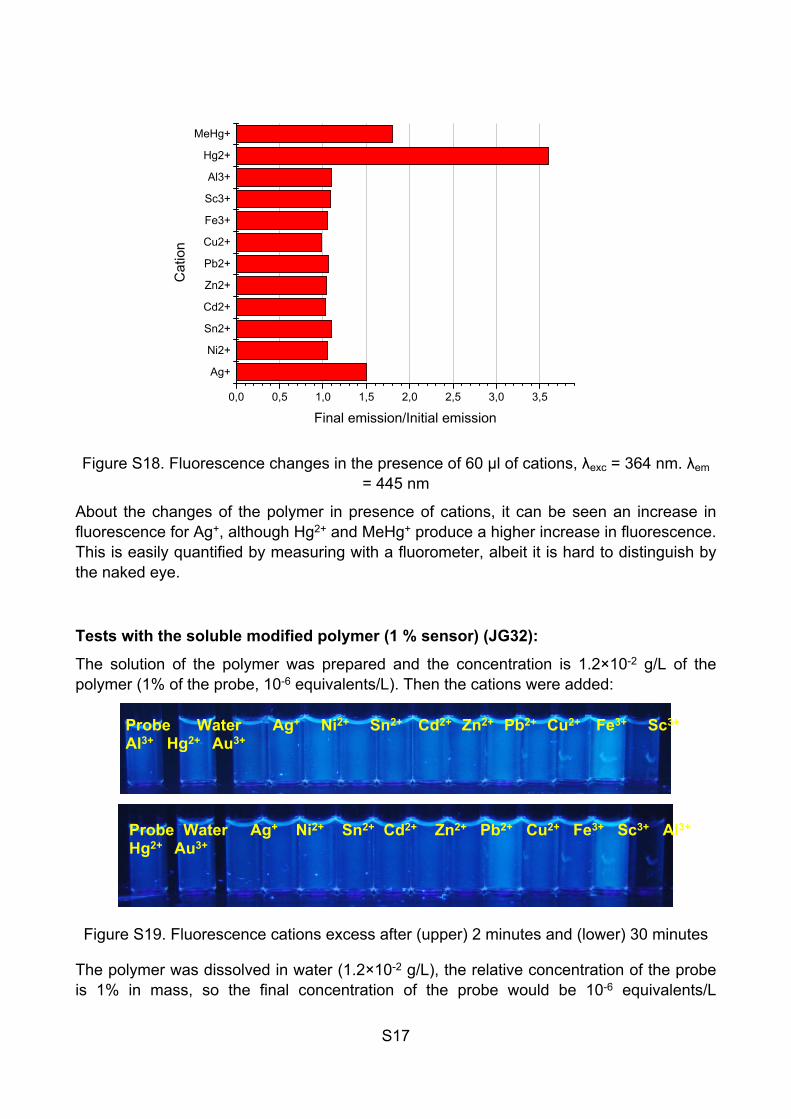
Figure S18. Fluorescence changes in the presence of 60 µl of cations, λexc = 364 nm. λem = 445 nm
About the changes of the polymer in presence of cations, it can be seen an increase in fluorescence for Ag+, although Hg2+ and MeHg+ produce a higher increase in fluorescence. This is easily quantified by measuring with a fluorometer, albeit it is hard to distinguish by the naked eye.
Tests with the soluble modified polymer (1 % sensor) (JG32):
The solution of the polymer was prepared and the concentration is 1.2×10⁻² g/L of the polymer (1% of the probe, 10-6 equivalents/L). Then the cations were added:
Figure S19. Fluorescence cations excess after (upper) 2 minutes and (lower) 30 minutes
The polymer was dissolved in water (1.2×10⁻² g/L), the relative concentration of the probe is 1% in mass, so the final concentration of the probe would be 10-6 equivalents/L
Probe Water Ag+ Ni2+ Sn2+ Cd2+ Zn2+ Pb2+ Cu2+ Fe3+ Sc3+ Al3+ Hg2+ Au3+
Probe Water Ag+ Ni2+ Sn2+ Cd2+ Zn2+ Pb2+ Cu2+ Fe3+ Sc3+ Al3+ Hg2+ Au3+
S18
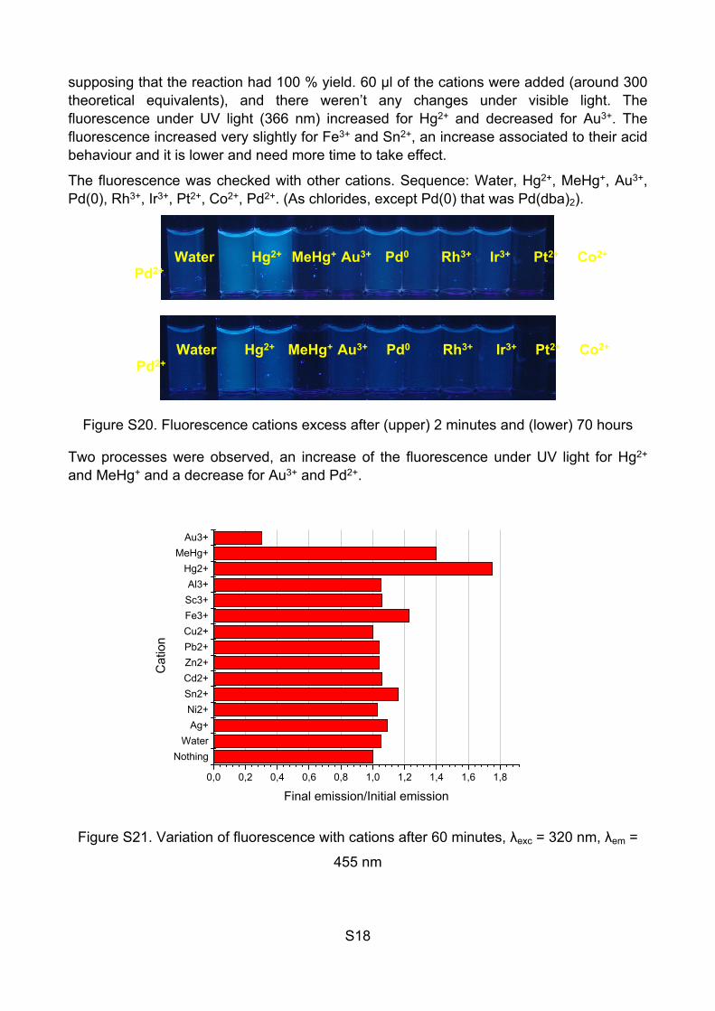
supposing that the reaction had 100 % yield. 60 µl of the cations were added (around 300 theoretical equivalents), and there weren’t any changes under visible light. The fluorescence under UV light (366 nm) increased for Hg2+ and decreased for Au3+. The fluorescence increased very slightly for Fe3+ and Sn2+, an increase associated to their acid behaviour and it is lower and need more time to take effect.
The fluorescence was checked with other cations. Sequence: Water, Hg2+, MeHg+, Au3+, Pd(0), Rh3+, Ir3+, Pt2+, Co2+, Pd2+. (As chlorides, except Pd(0) that was Pd(dba)2).
Figure S20. Fluorescence cations excess after (upper) 2 minutes and (lower) 70 hours
Two processes were observed, an increase of the fluorescence under UV light for Hg2+ and MeHg+ and a decrease for Au3+ and Pd2+.
NothingWater
Ag+Ni2+
Sn2+Cd2+Zn2+Pb2+Cu2+Fe3+Sc3+Al3+
Hg2+MeHg+
Au3+
0,0 0,2 0,4 0,6 0,8 1,0 1,2 1,4 1,6 1,8
Final emission/Initial emission
Cat
ion
Figure S21. Variation of fluorescence with cations after 60 minutes, λexc = 320 nm, λem =
455 nm
Water Hg2+ MeHg+ Au3+ Pd0 Rh3+ Ir3+ Pt2+ Co2+ Pd2+
Water Hg2+ MeHg+ Au3+ Pd0 Rh3+ Ir3+ Pt2+ Co2+ Pd2+
S19
NothingWater
Ag+Ni2+
Sn2+Cd2+Zn2+Pb2+Cu2+Fe3+Sc3+Al3+
Hg2+MeHg+
Au3+
0,0 0,2 0,4 0,6 0,8 1,0 1,2 1,4 1,6 1,8
Final emission/Initial emission
Cat
ion
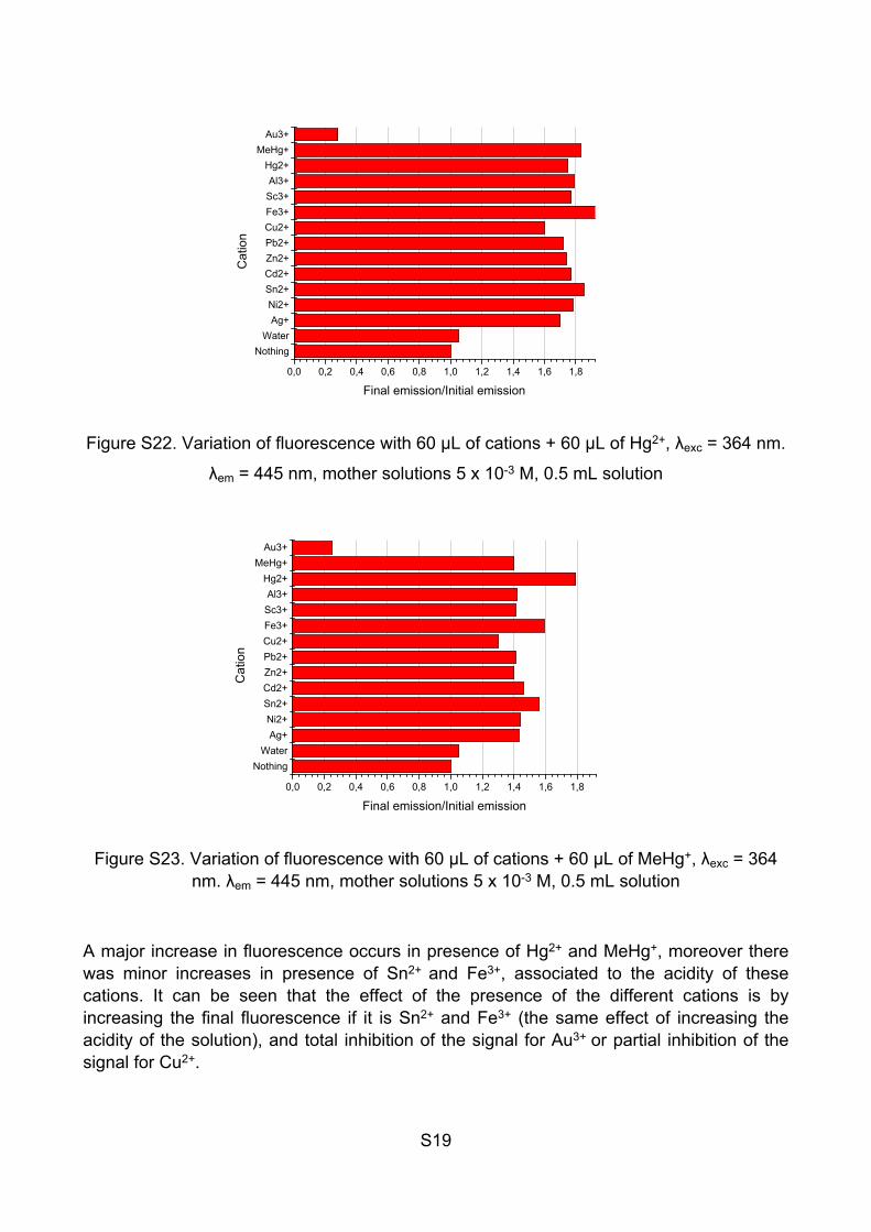
Figure S22. Variation of fluorescence with 60 µL of cations + 60 µL of Hg2+, λexc = 364 nm.
λem = 445 nm, mother solutions 5 x 10⁻³ M, 0.5 mL solution
NothingWater
Ag+Ni2+
Sn2+Cd2+Zn2+Pb2+Cu2+Fe3+Sc3+Al3+
Hg2+MeHg+
Au3+
0,0 0,2 0,4 0,6 0,8 1,0 1,2 1,4 1,6 1,8
Final emission/Initial emission
Cat
ion
Figure S23. Variation of fluorescence with 60 µL of cations + 60 µL of MeHg+, λexc = 364 nm. λem = 445 nm, mother solutions 5 x 10⁻³ M, 0.5 mL solution
A major increase in fluorescence occurs in presence of Hg2+ and MeHg+, moreover there was minor increases in presence of Sn2+ and Fe3+, associated to the acidity of these cations. It can be seen that the effect of the presence of the different cations is by increasing the final fluorescence if it is Sn2+ and Fe3+ (the same effect of increasing the acidity of the solution), and total inhibition of the signal for Au3+ or partial inhibition of the signal for Cu2+.
S20
QUANTITATIVE TESTS:
General conditions: Tests were carried out for the two synthesized polymers, the soluble in water (JG32) and the film with water affinity (JG25). Because of that, there are two procedures to measure in the fluorometer:
• In the case of solid polymers the sample was put between two magnetic sheets with a hole in the middle and placed in an angle of 45 degrees between the lamp and the detector (See the Figure S24). The concentration of analyte in the solution (in contact with the polymer) is successively increased in the cuvette and the changes in the fluorescence of the polymer are then measured.
• For the soluble polymer, a linear regression was necessary in order to find a concentration in which little variations change linearly the emission intensity and the absorbance.
Then the limit of detection of Hg2+ and MeHg+ was calculated, using the program “R” by following the next procedure:
• Adjusting to a mean square linear regression.
• Removing the “outliers”.
• Adjusting to a linear regression.
• Calculation of the LOD when the probability of false positive
and false negative is equal or inferior to 5 %.
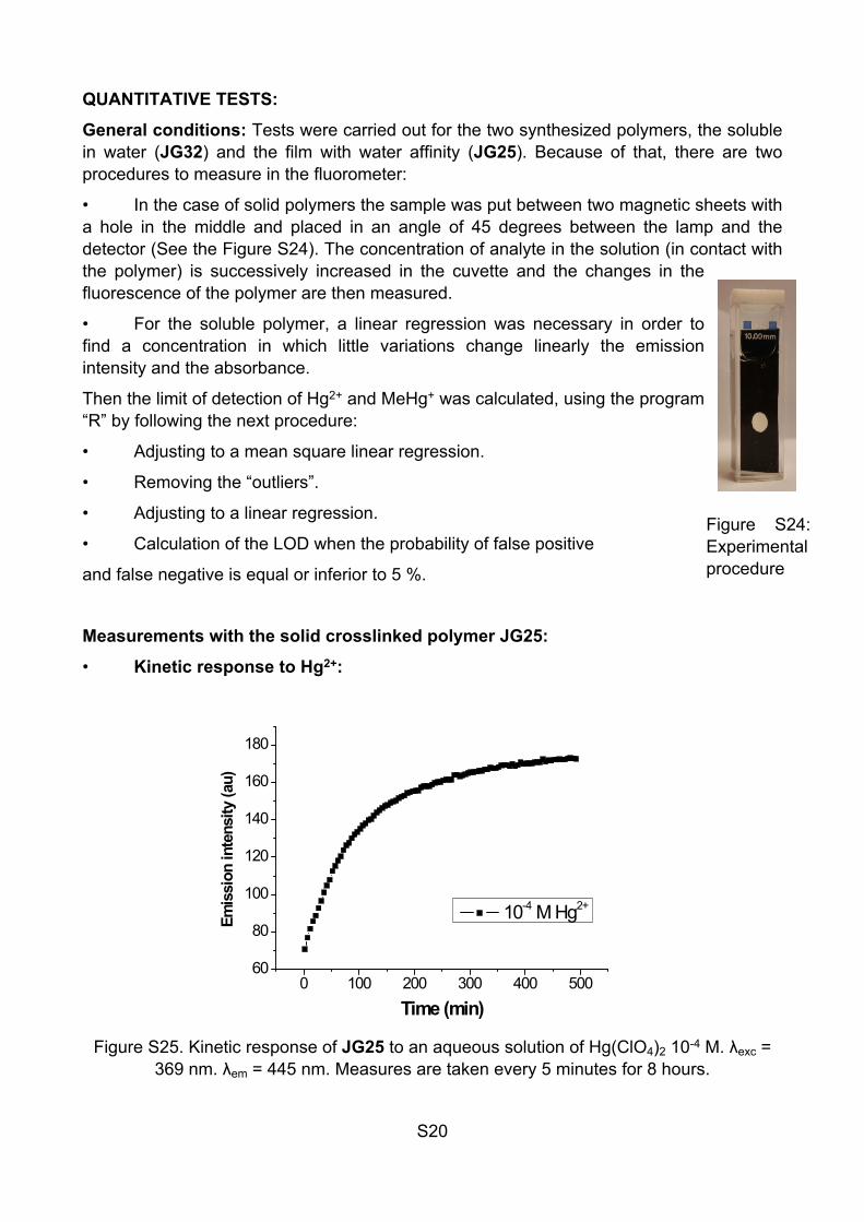
Measurements with the solid crosslinked polymer JG25:
• Kinetic response to Hg2+:
0 100 200 300 400 50060
80
100
120
140
160
180
Emis
sion
inte
nsity
(au)
Time (min)
10-4 M Hg2+
Figure S25. Kinetic response of JG25 to an aqueous solution of Hg(ClO4)2 10-4 M. λexc = 369 nm. λem = 445 nm. Measures are taken every 5 minutes for 8 hours.
Figure S24: Experimental procedure
S21
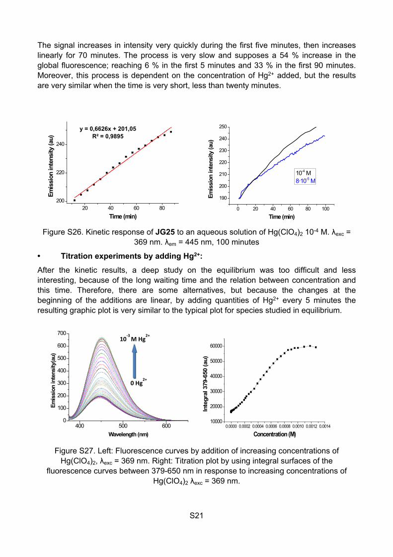
The signal increases in intensity very quickly during the first five minutes, then increases linearly for 70 minutes. The process is very slow and supposes a 54 % increase in the global fluorescence; reaching 6 % in the first 5 minutes and 33 % in the first 90 minutes. Moreover, this process is dependent on the concentration of Hg2+ added, but the results are very similar when the time is very short, less than twenty minutes.
20 40 60 80200
220
240
Emis
sion
inte
nsity
(au)
Time (min)0 20 40 60 80 100
190
200
210
220
230
240
250
Emis
sion
inte
nsity
(au)
Time (min)
10-4 M8·10-5 M
Figure S26. Kinetic response of JG25 to an aqueous solution of Hg(ClO4)2 10-4 M. λexc = 369 nm. λem = 445 nm, 100 minutes
• Titration experiments by adding Hg2+:
After the kinetic results, a deep study on the equilibrium was too difficult and less interesting, because of the long waiting time and the relation between concentration and this time. Therefore, there are some alternatives, but because the changes at the beginning of the additions are linear, by adding quantities of Hg2+ every 5 minutes the resulting graphic plot is very similar to the typical plot for species studied in equilibrium.
400 500 6000
100
200
300
400
500
600
700
Emis
sion
inte
nsity
(au)
Wavelength (nm)0.0000 0.0002 0.0004 0.0006 0.0008 0.0010 0.0012 0.0014
10000
20000
30000
40000
50000
60000
Inte
gral
379
-650
(au)
Concentration (M)
Figure S27. Left: Fluorescence curves by addition of increasing concentrations of Hg(ClO4)2, λexc = 369 nm. Right: Titration plot by using integral surfaces of the
fluorescence curves between 379-650 nm in response to increasing concentrations of Hg(ClO4)2 λexc = 369 nm.
y = 0,6626x + 201,05R² = 0,9895
10-3
M Hg2+
0 Hg2+
S22
In this way, the limit of detection obtained will be a little higher than taking measurements when the interaction Hg2+-probe reaches the equilibrium after a long time. But the value is perfectly valid for an assigned concentration and the time passed when that concentration was added. The saturation of the signal was reached when the concentration of Hg2+ was near 10-3 M (two hours and a half after the first addition) and, in a concentration below 10-5 M, the variation of intensity between additions was linear.
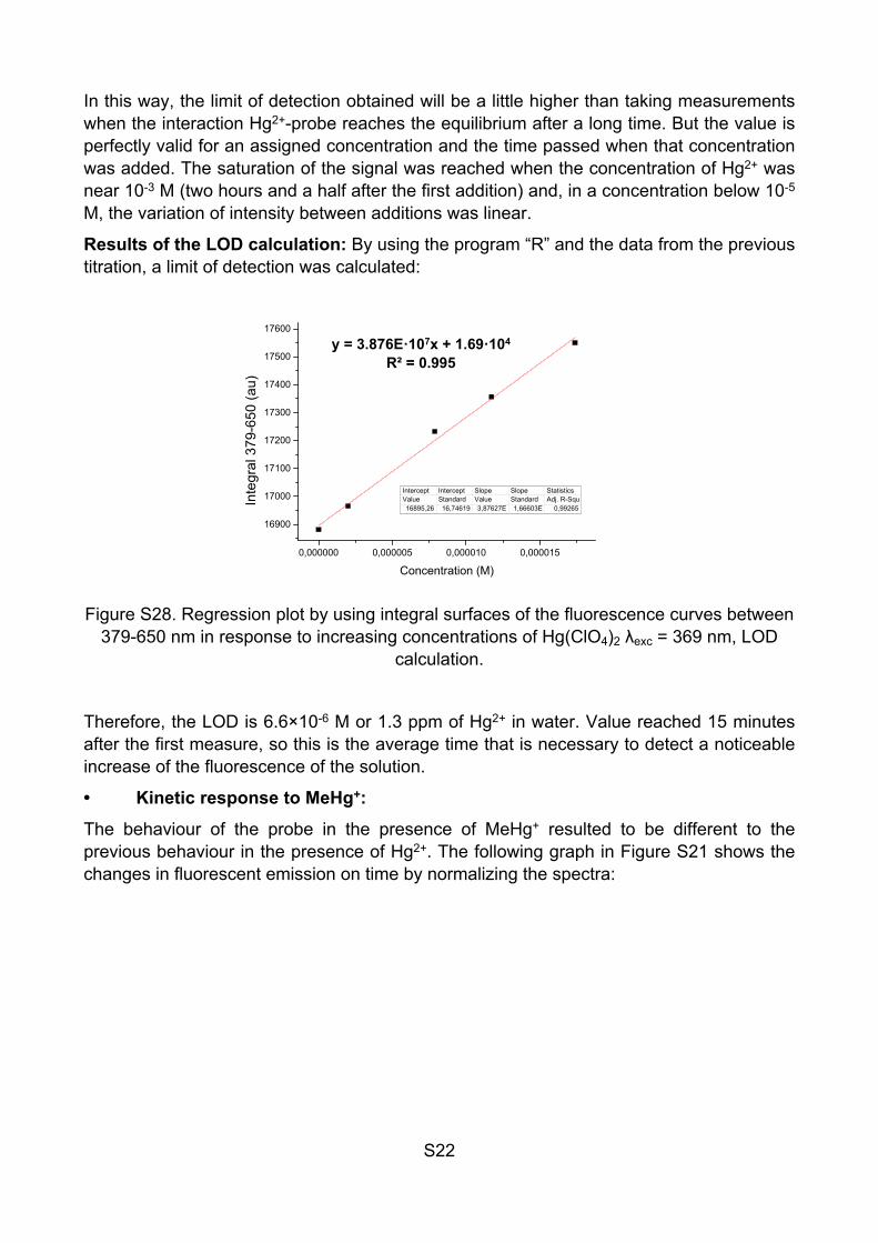
Results of the LOD calculation: By using the program “R” and the data from the previous titration, a limit of detection was calculated:
0,000000 0,000005 0,000010 0,000015
16900
17000
17100
17200
17300
17400
17500
17600
Inte
gral
379
-650
(au)
Concentration (M)
Intercept Intercept Slope Slope StatisticsValue Standard Value Standard Adj. R-Squ16895,26 16,74619 3,87627E 1,66603E 0,99265
Figure S28. Regression plot by using integral surfaces of the fluorescence curves between 379-650 nm in response to increasing concentrations of Hg(ClO4)2 λexc = 369 nm, LOD
calculation.
Therefore, the LOD is 6.6×10⁻⁶ M or 1.3 ppm of Hg2+ in water. Value reached 15 minutes after the first measure, so this is the average time that is necessary to detect a noticeable increase of the fluorescence of the solution.
• Kinetic response to MeHg+:
The behaviour of the probe in the presence of MeHg+ resulted to be different to the previous behaviour in the presence of Hg2+. The following graph in Figure S21 shows the changes in fluorescent emission on time by normalizing the spectra:
y = 3.876E·107x + 1.69·104
R² = 0.995
S23
0 200 400 600 8000,65
0,70
0,75
0,80
0,85
0,90
0,95
1,00
Emis
sion
inte
nsity
(au)
Time (min)
2.5·10-4 M10-4 M5·10-6 M
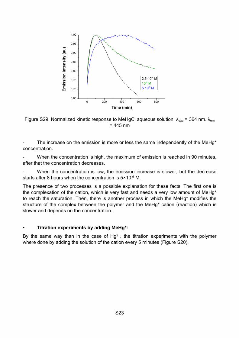
Figure S29. Normalized kinetic response to MeHgCl aqueous solution. λexc = 364 nm. λem = 445 nm
- The increase on the emission is more or less the same independently of the MeHg+ concentration.
- When the concentration is high, the maximum of emission is reached in 90 minutes, after that the concentration decreases.
- When the concentration is low, the emission increase is slower, but the decrease starts after 8 hours when the concentration is 5×10⁻⁶ M.
The presence of two processes is a possible explanation for these facts. The first one is the complexation of the cation, which is very fast and needs a very low amount of MeHg+ to reach the saturation. Then, there is another process in which the MeHg+ modifies the structure of the complex between the polymer and the MeHg+ cation (reaction) which is slower and depends on the concentration.
• Titration experiments by adding MeHg+:
By the same way than in the case of Hg2+, the titration experiments with the polymer where done by adding the solution of the cation every 5 minutes (Figure S20).

S24
400 450 500 550 600
0
50
100
150
200
250
300
350
400Em
issi
on in
tens
ity (a
u)
Wavelength (nm)0,00000 0,00005 0,00010 0,00015 0,00020
18000
20000
22000
24000
26000
28000
30000
32000
34000
Inte
gral
380
-650
(au)
Concentration (M)
Figure S30. Left: Fluorescence curves by addition of increasing concentrations of MeHgCl, λexc = 364 nm. Right: Titration plot by using integral surfaces of the fluorescence curves
between 380-650 nm in response to increasing concentrations of MeHgCl, λexc = 364 nm.
During the measurements the emission intensity increases faster than in the case of Hg2+.
Results of the LOD calculation:
0,000001 0,000002 0,00000318400
18600
18800
19000
19200
19400
19600
19800
Inte
gral
380
-650
(au)
Concentration (M)
Intercept Intercept Slope Slope StatisticsValue Standard Err Value Standard Err Adj. R-Squa
18308,3106 41,21094 4,5628E8 2,09196E7 0,98547
Figure S31. Regression plot by using integral surfaces of the fluorescence curves between 380-650 nm in response to increasing concentrations of MeHgCl, λexc = 364 nm. LOD
calculation.
Therefore the LOD is 1.5×10⁻⁶ M or 0.3 ppm. This value is reached in less than 20 minutes.
2·10-4 M

S25
• Effect of pH on JG25:
Although the quantitative measures were done in deionized water (pH = 8 approximately), it is important to study the pH effect on the samples in order to do further studies such as the measurements on fish samples, which are the final objective of the work.
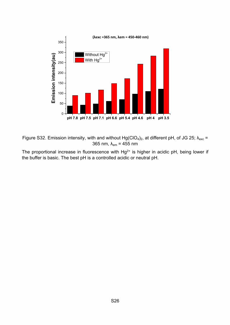
A cuvette buffered at pH = 7.8 (HEPES buffer, 5 mM) was acidified by adding 5 μL of HCl 1M and measuring the changes in pH and fluorescence. The results indicate that an increase of fluorescence is measured at lower pH. Then, by using the same process, the fluorescence increase was measured in a sample that contains 10-5 M of Hg2+.
Table S1: Emission intensity, with and without Hg(ClO4)2, at different pH, of JG25
pH Emission intensity (au) Emission intensity + Hg2+ (au)
7.8 39 89.2
7.5 43.5 100.6
7.1 49.4 116.7
6.6 60.9 148.4
5.4 69.7 173.0
4.6 96.4 243.0
4.0 110.1 282.7
3.5 121.9 318.7
S26
pH 7.8 pH 7.5 pH 7.1 pH 6.6 pH 5.4 pH 4.6 pH 4 pH 3.50
50
100
150
200
250
300
350
Emis
sion
inte
nsity
(au) Without Hg2+
With Hg2+
Figure S32. Emission intensity, with and without Hg(ClO4)2, at different pH, of JG 25; λexc = 365 nm, λem = 455 nm
The proportional increase in fluorescence with Hg2+ is higher in acidic pH, being lower if the buffer is basic. The best pH is a controlled acidic or neutral pH.
(λexc =365 nm, λem = 450-460 nm)
S27
Measurements with the soluble polymer JG32:
• Work concentration calculation:
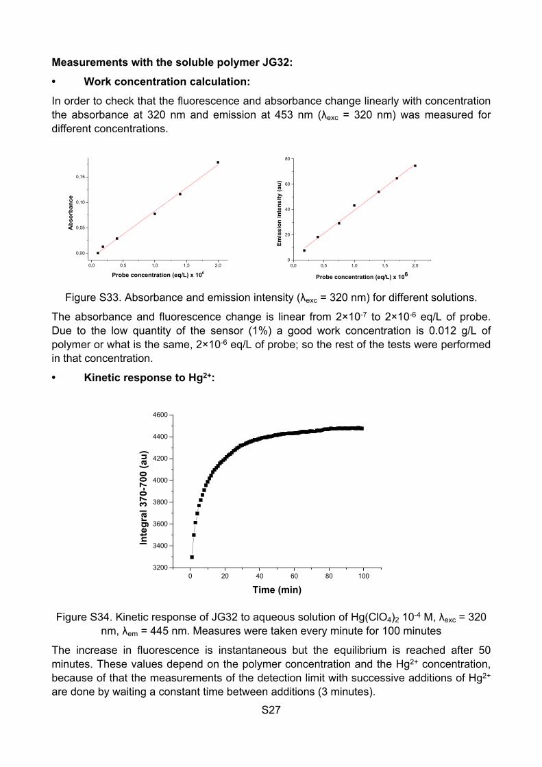
In order to check that the fluorescence and absorbance change linearly with concentration the absorbance at 320 nm and emission at 453 nm (λexc = 320 nm) was measured for different concentrations.
0,0 0,5 1,0 1,5 2,0
0,00
0,05
0,10
0,15
Abs
orba
nce
Probe concentration (eq/L) x 106
0,0 0,5 1,0 1,5 2,00
20
40
60
80
Emis
sion
inte
nsity
(au)
Probe concentration (eq/L) x 106
Figure S33. Absorbance and emission intensity (λexc = 320 nm) for different solutions.
The absorbance and fluorescence change is linear from 2×10⁻⁷ to 2×10⁻⁶ eq/L of probe. Due to the low quantity of the sensor (1%) a good work concentration is 0.012 g/L of polymer or what is the same, 2×10⁻⁶ eq/L of probe; so the rest of the tests were performed in that concentration.
• Kinetic response to Hg2+:
0 20 40 60 80 1003200
3400
3600
3800
4000
4200
4400
4600
Inte
gral
370
-700
(au)
Time (min)
Figure S34. Kinetic response of JG32 to aqueous solution of Hg(ClO4)2 10-4 M, λexc = 320 nm, λem = 445 nm. Measures were taken every minute for 100 minutes
The increase in fluorescence is instantaneous but the equilibrium is reached after 50 minutes. These values depend on the polymer concentration and the Hg2+ concentration, because of that the measurements of the detection limit with successive additions of Hg2+ are done by waiting a constant time between additions (3 minutes).
S28
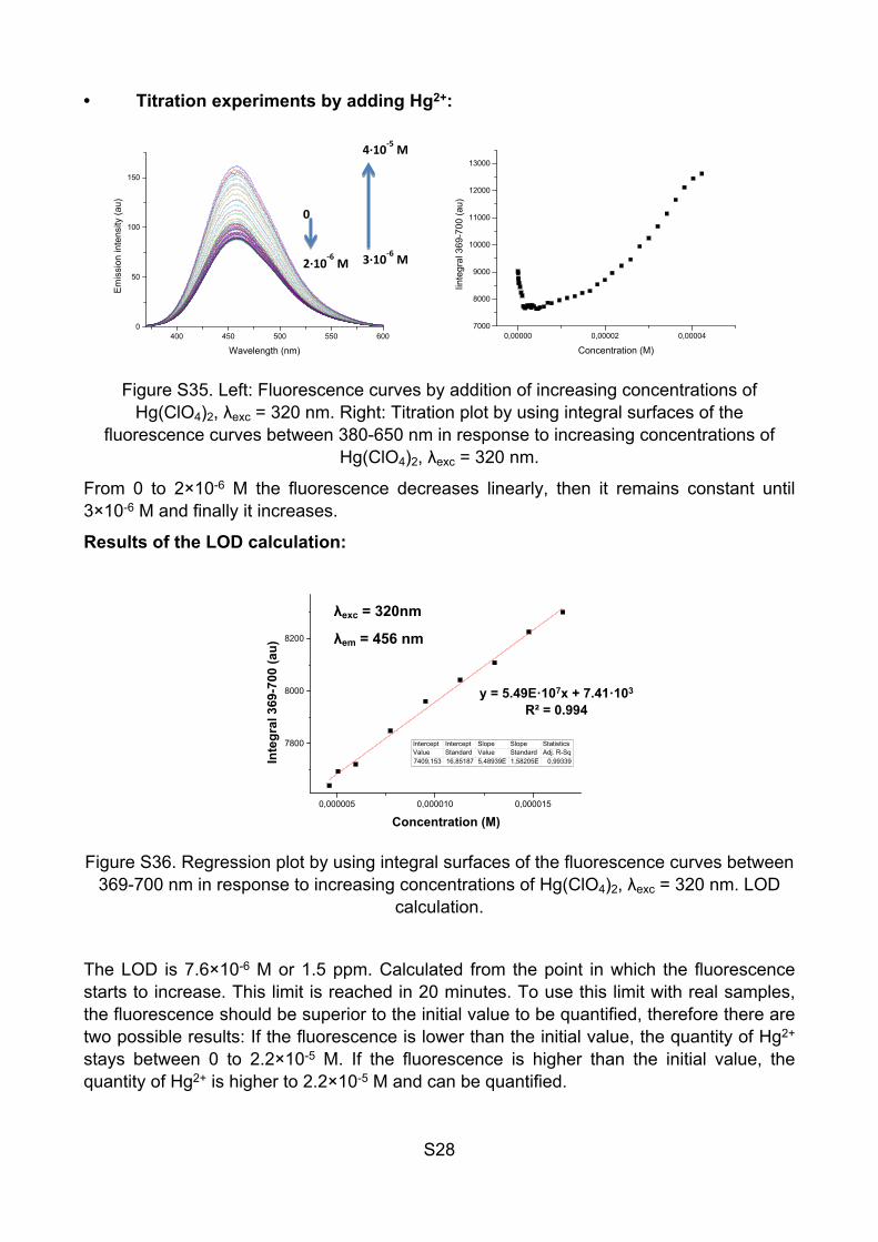
• Titration experiments by adding Hg2+:
400 450 500 550 6000
50
100
150
Em
issi
on in
tens
ity (a
u)
Wavelength (nm)0,00000 0,00002 0,00004
7000
8000
9000
10000
11000
12000
13000
Iinte
gral
369
-700
(au)
Concentration (M)
Figure S35. Left: Fluorescence curves by addition of increasing concentrations of Hg(ClO4)2, λexc = 320 nm. Right: Titration plot by using integral surfaces of the
fluorescence curves between 380-650 nm in response to increasing concentrations of Hg(ClO4)2, λexc = 320 nm.
From 0 to 2×10⁻⁶ M the fluorescence decreases linearly, then it remains constant until 3×10⁻⁶ M and finally it increases.
Results of the LOD calculation:
0,000005 0,000010 0,000015
7800
8000
8200
Inte
gral
369
-700
(au)
Concentration (M)
Intercept Intercept Slope Slope StatisticsValue Standard Value Standard Adj. R-Sq7409,153 16,85187 5,48939E 1,58205E 0,99339
Figure S36. Regression plot by using integral surfaces of the fluorescence curves between 369-700 nm in response to increasing concentrations of Hg(ClO4)2, λexc = 320 nm. LOD
calculation.
The LOD is 7.6×10⁻⁶ M or 1.5 ppm. Calculated from the point in which the fluorescence starts to increase. This limit is reached in 20 minutes. To use this limit with real samples, the fluorescence should be superior to the initial value to be quantified, therefore there are two possible results: If the fluorescence is lower than the initial value, the quantity of Hg2+ stays between 0 to 2.2×10⁻⁵ M. If the fluorescence is higher than the initial value, the quantity of Hg2+ is higher to 2.2×10⁻⁵ M and can be quantified.
4·10-5 M
3·10-6 M
0
2·10-6
M
λexc = 320nm
λem = 456 nm
y = 5.49E·107x + 7.41·103
R² = 0.994

S29
For this polymer there is a clear second effect of decreasing the fluorescence when the concentration is very low. Without more data this effect could be associated to a kinetic effect. To check that effect, some solutions near the LOD were prepared and the fluorescence was measured at different times.
0,000000 0,000002 0,000004 0,000006 0,000008 0,000010
108
110
112
114
116
118
120
122
124
90 minutes4 hours
Emis
sion
inte
nsity
(au)
Hg2+ Concentration (M)
Figure S37. Emission intensity difference at low concentrations of Hg(ClO4)2 at different times, λexc = 320 nm.
The analysis of the graph leads to the conclusion that the results under low concentrations barely change. This behaviour was checked three times giving similar results.
• Kinetic response to MeHg+:
0 10 20 30 40 500
10
20
30
40
50
Emis
sion
inte
nsity
(au)
Time (min)
Hg2+ (4·10-5 M) MeHg+ (4·10-5 M) MeHg+ (8·10-5 M) MeHg+ (1.2·10-4 M)
Figure S38. Kinetic response of JG32 to aqueous solutions of Hg(ClO4)2 and MeHgCl at different concentrations, λexc = 320 nm, λem = 456 nm. Measures were taken for 55
minutes.
λexc = 320nm
λem = 456 nm
λexc = 320nm
λem = 454 nm
S30
The increase in fluorescence is faster with MeHg+ at the beginning, the first 5 minutes, but the maximum is reached more slowly and the final fluorescence is lower at the same concentration of each species.
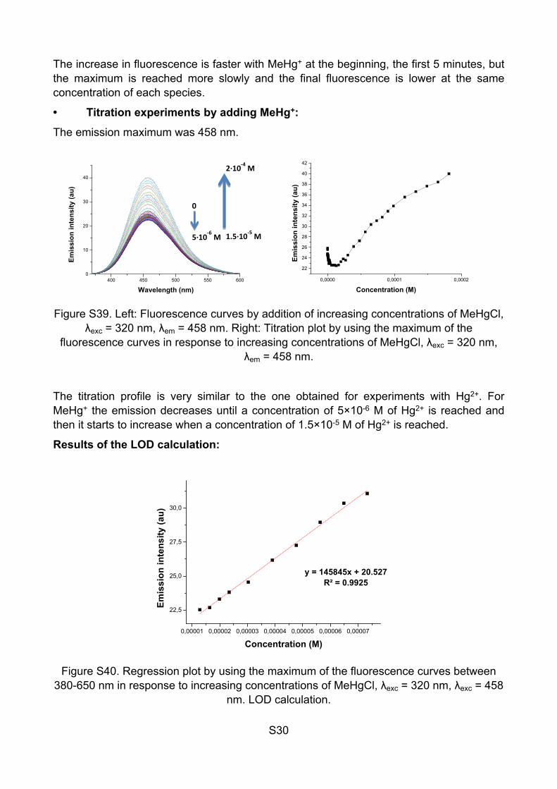
• Titration experiments by adding MeHg+:
The emission maximum was 458 nm.
400 450 500 550 6000
10
20
30
40
Emis
sion
inte
nsity
(au)
Wavelength (nm)0,0000 0,0001 0,0002
22
24
26
28
30
32
34
36
38
40
42
Emis
sion
inte
nsity
(au)
Concentration (M)
Figure S39. Left: Fluorescence curves by addition of increasing concentrations of MeHgCl, λexc = 320 nm, λem = 458 nm. Right: Titration plot by using the maximum of the
fluorescence curves in response to increasing concentrations of MeHgCl, λexc = 320 nm, λem = 458 nm.
The titration profile is very similar to the one obtained for experiments with Hg2+. For MeHg+ the emission decreases until a concentration of 5×10⁻⁶ M of Hg2+ is reached and then it starts to increase when a concentration of 1.5×10⁻⁵ M of Hg2+ is reached.
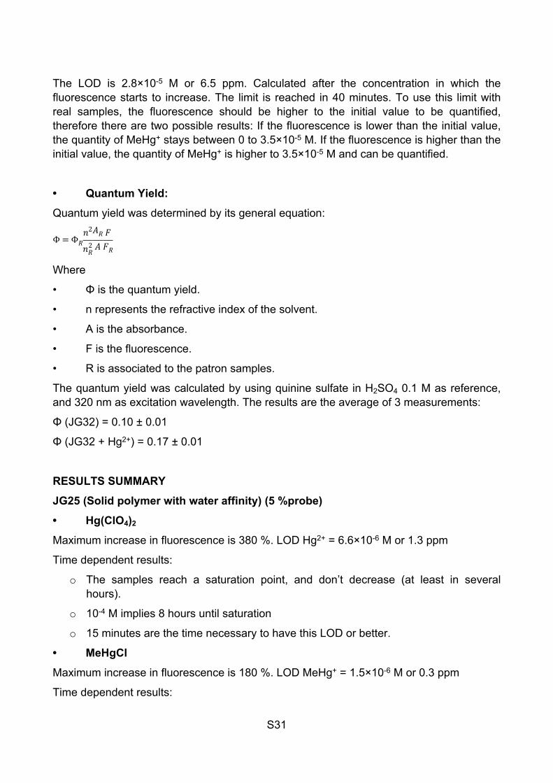
Results of the LOD calculation:
0,00001 0,00002 0,00003 0,00004 0,00005 0,00006 0,00007
22,5
25,0
27,5
30,0
Emis
sion
inte
nsity
(au)
Concentration (M)
Figure S40. Regression plot by using the maximum of the fluorescence curves between 380-650 nm in response to increasing concentrations of MeHgCl, λexc = 320 nm, λexc = 458
nm. LOD calculation.
2·10-4 M
1.5·10-5 M
0
5·10-6
M
y = 145845x + 20.527R² = 0.9925
S31
The LOD is 2.8×10⁻⁵ M or 6.5 ppm. Calculated after the concentration in which the fluorescence starts to increase. The limit is reached in 40 minutes. To use this limit with real samples, the fluorescence should be higher to the initial value to be quantified, therefore there are two possible results: If the fluorescence is lower than the initial value, the quantity of MeHg+ stays between 0 to 3.5×10⁻⁵ M. If the fluorescence is higher than the initial value, the quantity of MeHg+ is higher to 3.5×10⁻⁵ M and can be quantified.
• Quantum Yield:
Quantum yield was determined by its general equation:
Φ=Φ𝑅𝑛2
𝑛2𝑅
𝐴𝑅𝐴𝐹𝐹𝑅
Where
• Φ is the quantum yield.
• n represents the refractive index of the solvent.
• A is the absorbance.
• F is the fluorescence.
• R is associated to the patron samples.
The quantum yield was calculated by using quinine sulfate in H2SO4 0.1 M as reference, and 320 nm as excitation wavelength. The results are the average of 3 measurements:
Φ (JG32) = 0.10 ± 0.01
Φ (JG32 + Hg2+) = 0.17 ± 0.01
RESULTS SUMMARY
JG25 (Solid polymer with water affinity) (5 %probe)
• Hg(ClO4)2
Maximum increase in fluorescence is 380 %. LOD Hg2+ = 6.6×10⁻⁶ M or 1.3 ppm
Time dependent results:
o The samples reach a saturation point, and don’t decrease (at least in several hours).
o 10-4 M implies 8 hours until saturation
o 15 minutes are the time necessary to have this LOD or better.
• MeHgCl
Maximum increase in fluorescence is 180 %. LOD MeHg+ = 1.5×10⁻⁶ M or 0.3 ppm
Time dependent results:

S32
o The fluorescence increases and when the maximum is reached it starts to decrease.
o Higher concentrations imply faster increase of the fluorescence, but once reached the maximum it decreases faster.
o The maximum of fluorescence is not higher when the concentration is higher than 5×10⁻⁶ M.
o The maximum of fluorescence is reached faster than with Hg2+ 90 minutes at high concentrations and less than 3 hours with 5×10⁻⁶ M.
o The increase in fluorescence is lower than with Hg2+.
o 20 minutes is enough to have a good reproducibility of this LOD.
• The pH changes the response to Hg2+ by increasing the emission intensity when the pH is lower, but the initial emission of the polymer is also higher.
JG32 (polymer soluble in water) (1 % probe) 0.012 g/L
Φ (JG32) = 0.10 ± 0.01
Φ (JG32 + Hg2+) = 0.17 ± 0.01
• Hg(ClO4)2
Maximum increase in fluorescence is 177 %. LOD Hg2+ = 2.2·10-5 M or 4.4 ppm.
Time dependent results:
o The samples reach a maximum fluorescence value that then does not decrease (at least within 100 minutes).
o A concentration 10-4 M needs 50 minutes until maximum value of fluorescence is reached.
o To have a reliable LOD the time necessary for measurements is 20 minutes.
The fluorescence starts to increase when the concentration is higher than 2×10⁻⁶ M, and this process is independent of time.
• MeHgCl
Maximum increase in fluorescence 160 % from the minimum, 140 % from the initial fluorescence. LOD MeHg+ = 3.9×10⁻⁵ M or 7.5 ppm
Time dependent results:
o The fluorescence increases faster than with Hg2+ within the first 5 minutes.
o The final increase in fluorescence is lower than with Hg2+.
o 40 minutes is enough to have a good reproducibility of the LOD.
The fluorescence starts to increase when the concentration is higher than 5×10⁻⁶ M, and this process is not time-dependent.

S33
ANALYSIS OF FISH SAMPLES
FishSamples
Lyophilization
ExtractionDirect
Measures
AcidExtraction
SilicaExtraction
ICP Fluorescence ICP Fluorescence Fluorescence
Normalization of Fluorescence
ResultsComparison
Figure S41: A scheme of treatment for analysis of fish samples.
In order to find the best conditions to have reproducible and reliable measures of the presence of mercury in fish samples, some preliminary tests are necessary:
• To measure the mercury extracted from the fish samples by ICP-mass analysis.
• Qualitative measures of the fluorescent changes of the polymer in the presence of the mercury extracts.
• Measurements of some different fish samples.
Analysis of mercury extracted from fish samples:
a) Extraction of mercury species from fish
Two methods were tested: acidic extraction and silica extraction. The basic extraction was discarded because of the high temperatures, the extracts are colored and the probe has no good results at pH superior than 8 so it had interferences in fluorescence measures. All the measurements were done with lyophilized fish because the quantity of water is vital in the concentration calculation.
Acid extraction: 5 ml of HCl 5 M in water and 5 ml of NaCl 0.25 M in water were added to 0.5 g of lyophilized fish in a microwave Owen vial. The mixture was sonicated for 10 minutes and heated for 10 minutes at 60 ºC in the microwave Owen. Then the mixture was centrifuged at 4000 rpm for 10 minutes and at 7000 rpm for additional 10 minutes. The liquid phase was filtered in a glass fibre filter of 0.22 μm pore. Finally, the samples to be measured by fluorescence were concentrated to 1 ml.
Silica extraction: 0.5 g of fish and 2 ml of water were mixed in a mortar and the mixture was grinded, 1g of silica was then added and mixed. The mixture was then treated with HCl 5 M in water following the same procedure used for the acid extraction, but without using the microwave Owen. Finally, the samples to be measured by fluorescence were concentrated to 1 ml.
S34
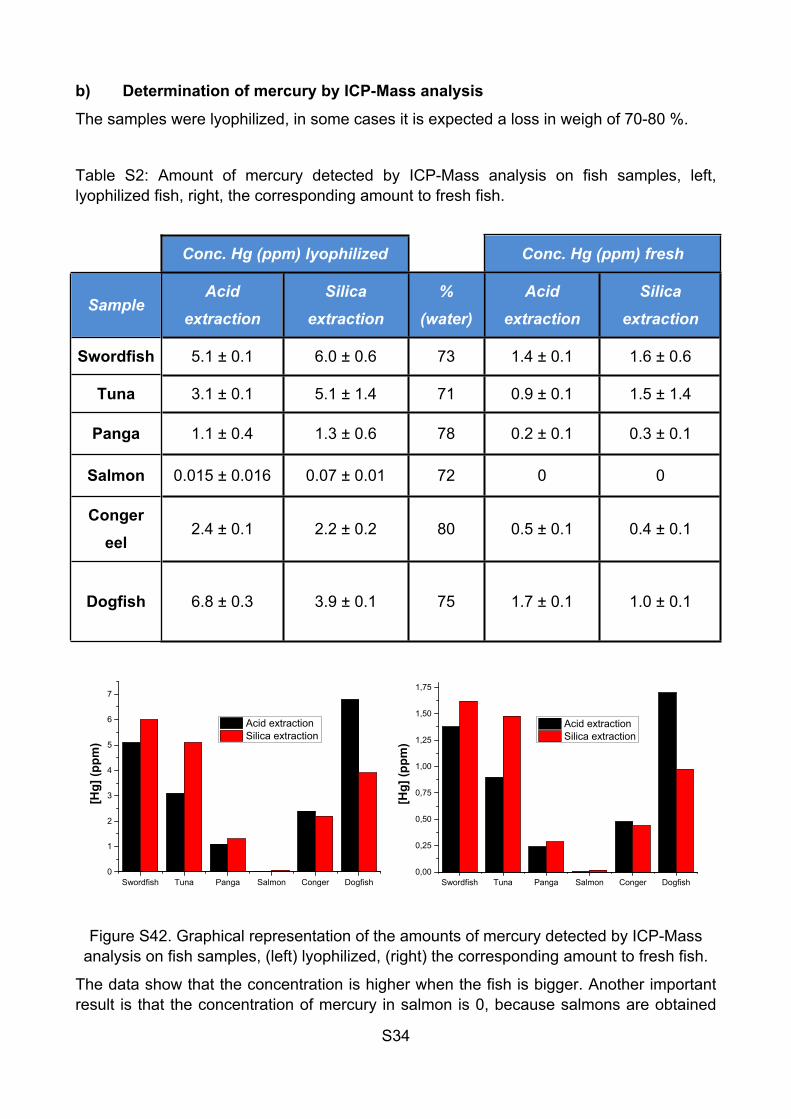
b) Determination of mercury by ICP-Mass analysis
The samples were lyophilized, in some cases it is expected a loss in weigh of 70-80 %.
Table S2: Amount of mercury detected by ICP-Mass analysis on fish samples, left, lyophilized fish, right, the corresponding amount to fresh fish.
Conc. Hg (ppm) lyophilized Conc. Hg (ppm) fresh
SampleAcid
extractionSilica
extraction%
(water)Acid
extractionSilica
extraction
Swordfish 5.1 ± 0.1 6.0 ± 0.6 73 1.4 ± 0.1 1.6 ± 0.6
Tuna 3.1 ± 0.1 5.1 ± 1.4 71 0.9 ± 0.1 1.5 ± 1.4
Panga 1.1 ± 0.4 1.3 ± 0.6 78 0.2 ± 0.1 0.3 ± 0.1
Salmon 0.015 ± 0.016 0.07 ± 0.01 72 0 0
Conger eel
2.4 ± 0.1 2.2 ± 0.2 80 0.5 ± 0.1 0.4 ± 0.1
Dogfish 6.8 ± 0.3 3.9 ± 0.1 75 1.7 ± 0.1 1.0 ± 0.1
Swordfish Tuna Panga Salmon Conger Dogfish0
1
2
3
4
5
6
7
[Hg]
(ppm
)
Acid extraction Silica extraction
Swordfish Tuna Panga Salmon Conger Dogfish0,00
0,25
0,50
0,75
1,00
1,25
1,50
1,75
[Hg]
(ppm
)
Acid extraction Silica extraction
Figure S42. Graphical representation of the amounts of mercury detected by ICP-Mass analysis on fish samples, (left) lyophilized, (right) the corresponding amount to fresh fish.
The data show that the concentration is higher when the fish is bigger. Another important result is that the concentration of mercury in salmon is 0, because salmons are obtained
S35
from a fish farm, not from the sea, so the concentration of mercury is 0. The concentrations of mercury in swordfish, tuna, conger eel and dogfish are high enough to be measured with the solid polymer and, in case of swordfish, around the maximum amount per week recommended by the FDA, (1.3 ppm). The LOD of the polymer JG25 is 1.3 ppm for Hg2+ and 0.3 ppm for MeHg+, therefore a direct measure is possible, depending on the possible interferents. In any case, we started by making an extraction and checking the results.
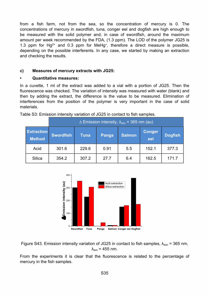
c) Measures of mercury extracts with JG25:
• Quantitative measures:
In a cuvette, 1 ml of the extract was added to a vial with a portion of JG25. Then the fluorescence was checked. The variation of intensity was measured with water (blank) and then by adding the extract, the difference is the value to be measured. Elimination of interferences from the position of the polymer is very important in the case of solid materials.
Table S3: Emission intensity variation of JG25 in contact to fish samples.
∆ Emission intensity, λexc = 365 nm (au)
Extraction Method
Swordfish Tuna Panga SalmonConger
eelDogfish
Acid 301.6 229.6 0.91 5.5 152.1 377.3
Silica 354.2 307.2 27.7 6.4 162.5 171.7
Swordfish Tuna Panga Salmon Conger eel Dogfish0
100
200
300
400
E
mis
sion
inte
nsity
(au) Acid extraction
Silica extraction
Figure S43. Emission intensity variation of JG25 in contact to fish samples, λexc = 365 nm, λem = 455 nm.
From the experiments it is clear that the fluorescence is related to the percentage of mercury in the fish samples.
S36
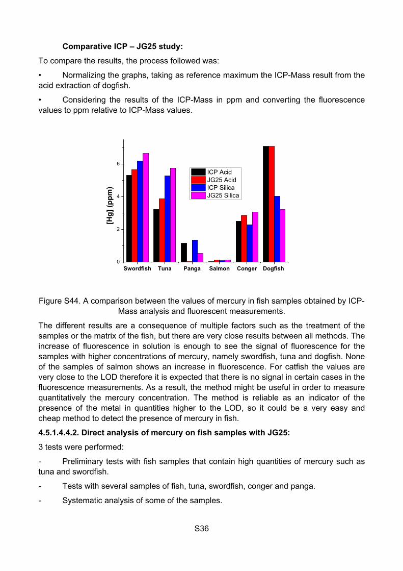
Comparative ICP – JG25 study:
To compare the results, the process followed was:
• Normalizing the graphs, taking as reference maximum the ICP-Mass result from the acid extraction of dogfish.
• Considering the results of the ICP-Mass in ppm and converting the fluorescence values to ppm relative to ICP-Mass values.
Swordfish Tuna Panga Salmon Conger Dogfish 0
2
4
6
[Hg]
(ppm
)
ICP Acid JG25 Acid ICP Silica JG25 Silica
Figure S44. A comparison between the values of mercury in fish samples obtained by ICP-Mass analysis and fluorescent measurements.
The different results are a consequence of multiple factors such as the treatment of the samples or the matrix of the fish, but there are very close results between all methods. The increase of fluorescence in solution is enough to see the signal of fluorescence for the samples with higher concentrations of mercury, namely swordfish, tuna and dogfish. None of the samples of salmon shows an increase in fluorescence. For catfish the values are very close to the LOD therefore it is expected that there is no signal in certain cases in the fluorescence measurements. As a result, the method might be useful in order to measure quantitatively the mercury concentration. The method is reliable as an indicator of the presence of the metal in quantities higher to the LOD, so it could be a very easy and cheap method to detect the presence of mercury in fish.
4.5.1.4.4.2. Direct analysis of mercury on fish samples with JG25:
3 tests were performed:
- Preliminary tests with fish samples that contain high quantities of mercury such as tuna and swordfish.
- Tests with several samples of fish, tuna, swordfish, conger and panga.
- Systematic analysis of some of the samples.

S37
• Test 1:
Three pieces of polymer (JG25) were placed in contact to three new fish samples containing fresh tuna, fresh swordfish, and a mixture of swordfish+Hg2+. Every fish sample, 2 g, was grinded and mixed with 5 ml of water and then left in contact with a polymer fragment. After a period of time the polymer fragment was taken from the solution and dried in order to compare the fluorescence of every polymer fragment. Previously, by ICP-Mass, the samples of fresh fish showed that tuna had a concentration of 0.7 ± 0.1 ppm and swordfish had a concentration of 3.7 ± 0.8 ppm. After one hour the difference between the fish samples and the blank is clear and correlates quite well with the real amounts of mercury present in every sample. But after one day in contact the increase is even higher. This analysis was a preliminary test in order to check the possibility of these kinds of measures, because of that it was repeated with more polymer fragments and more fish samples in order to compare the results of fish samples with high and low amounts of mercury.
• Test 2:
Four pieces of polymer (JG25) were put in presence of four new fish samples containing: tuna – swordfish – conger – panga. Qualitatively, the only clear difference is noticed between the blank and the panga with no fluorescence and low fluorescence respectively. The polymer fragment with added Hg2+ is the most fluorescent and the rest of the samples give variations in fluorescence that cannot be evaluated quantitatively by the naked eye, but may give a clear qualitative evaluation of the presence or absence of mercury in the fish samples.
• Test 3:
In this case, we used the same samples originally used for extractions, in order to compare the results with fish samples and extracts, taking in account the large variability of mercury contamination between different fish samples from different specimens, from them, 0.5 g of lyophilized fish samples were mixed with 2 ml of water. Then a piece of the polymeric sensor was added. To check the difference in fluorescence every polymer fragment in contact with fish samples was measured at different waiting times in the fluorometer, obtaining the results in Table S4 and Figure S26. The results can be compared with the corresponding results from the extraction by normalizing to one of them (dogfish in this case) (Figure S27).
Table S4: The relation between the concentration of mercury and the obtained values of fluorescence for fish samples and the polymeric sensor.
∆ Emission intensity 365 nm (au)
Sample/ time (h) Swordfish Tuna Panga Conger eel Dogfish
0.5 220.5 212.2 21.3 32.0 230.93
1 260.8 237.7 21.97 65.79 272.2
24 301.6 280.0 30.68 136.3 318.4

S38
Swordfish Tuna Panga Conger Dogfish0
50
100
150
200
250
300
350
E
mis
ssio
n in
tens
ity (a
u)
30 minutes60 minutes24 hours
Figure S45. Emission intensity variation with fresh fish samples (λexc = 365 nm, λem = 455 nm) at different waiting times.
Swordfish Tuna Panga Conger Dogfish 0,0
0,5
1,0
1,5
2,0
[Hg]
(ppm
)
ICP Acid JG25 Acid ICP Silica JG25 Silica JG25 Fresh
Figure S46. Emission intensity variation in experiments with fresh fish samples (λexc = 365 nm, λem = 455 nm) compared with the results from the extracts.
Therefore, a relation between the concentration of mercury and the obtained values of fluorescence is confirmed.