a smooth, three-surface elasto-plastic cap model: rate formulation
TRANSCRIPT

A Smooth, Three-Surface Elasto-PlasticCap Model: Rate Formulation, Integration
Algorithm and Tangent Operators
Colby C. Swan4120 Seamans Center for Engineering Arts & Sciences
Department of Civil and Environmental EngineeringCenter for Computer-Aided Design
The University of IowaIowa City, Iowa 52242, USA
E-mail: [email protected] : 1(319) 335-5831
Young-Kyo Seo, Post-Doctoral Research AssociateDepartment of Civil and Environmental Engineering
Computational Solid Mechanics LaboratoryThe University of Iowa
Iowa City, Iowa 52242, USAE-mail: [email protected]
Phone : 1(319) 335-6455
Abstract
One of the primary strengths of elasto-plastic cap models is their ability to capture the gross inelasticcoupling between deviatoric and volumetric behaviors of many porous media. While numericalintegration algorithms for these models have been presented in the literature, performing implicitanalysis of earthen systems using cap models remains a challenging endeavor. One of the difficultiesassociated with most isotropic cap models is that the three independent surfaces comprising theyield surface intersect non-smoothly. It is shown here that the elastoplastic tangent operators atthe corner points on such yield surfaces are singular, giving rise to potential numerical difficulties.To address this issue, a novel, three-surface elasto-plastic cap model in which the three surfacesintersect smoothly is introduced and developed here. The rate form of the model constitutiveequations are first presented, followed by an unconditionally stable integration algorithm withexpressions for consistent tangent operators. Sample computations demonstrating the very goodperformance of the model in slope stability and bearing capacity problems are also presented.
Key words: cap models; elasto-plasticity; soil models; computational plasticity;
Table of Contents
Page
1. INTRODUCTION . . . . . . . . . . . . . . . . . . . . . . . . . . . . 1
2. ASSESSMENT OF A NON-SMOOTH CAP MODELS . . . . . . . . . . . . . 4
2.1 Basic Forms and Rate Equations . . . . . . . . . . . . . . . . . . 4
2.2 The Problem: Singular Tangent Operators at Corner Points . . . . . . . 7
3. INTRODUCTION OF A NOVEL, SMOOTH CAP MODEL . . . . . . . . . . . 9
3.1 Basic Forms and Rate Equations . . . . . . . . . . . . . . . . . . 9
3.2 Determination of Compression Cap Radius . . . . . . . . . . . . 12
3.3 Stress Updates and Active Yield Surface Determination . . . . . . . 13
3.4 Case 1 Integration Algorithm . . . . . . . . . . . . . . . . . . 16
3.5 Case 2 Integration Algorithm . . . . . . . . . . . . . . . . . . 19
3.6 Case 3 Integration Algorithm . . . . . . . . . . . . . . . . . . 23
3.7 Consistent Tangent Operators . . . . . . . . . . . . . . . . . . 25
4. EXAMPLE COMPUTATIONS . . . . . . . . . . . . . . . . . . . . . . 27
4.1 Hydrostatic Compression Test . . . . . . . . . . . . . . . . . . 27
4.2 A Four Element Limit Analysis Computation . . . . . . . . . . . 29
4.3 Bearing Capacity Computations . . . . . . . . . . . . . . . . . 30
4.4 Slope Stability Analysis Computations . . . . . . . . . . . . . . 31
5. SUMMARY AND CLOSURE . . . . . . . . . . . . . . . . . . . . . . 32
6. ACKNOWLEDGEMENTS . . . . . . . . . . . . . . . . . . . . . . . 33
7. BIBLIOGRAPHY . . . . . . . . . . . . . . . . . . . . . . . . . . . 33
ii

Page
List of Figures
1. Non-smooth, three-surface, two-invariant cap model yield surface with twocorner points . . . . . . . . . . . . . . . . . . . . . . . . . . . . . . 2
2. Smooth, three-surface two-invariant yield function for cap model . . . . . . . 10
3. Possible Case 1 return conditions when� tr
1 � 0 . . . . . . . . . . . . . . . 17
4. Potential yield surace activity when� tr
1 � 0 . . . . . . . . . . . . . . . . 17
5. Single element hydrostatic compression test . . . . . . . . . . . . . . . . 28
6. Four-element limit state analysis computation . . . . . . . . . . . . . . . 29
7. Mesh and results of rigid foundation bearing capacity computations on looseand dense sandy soils . . . . . . . . . . . . . . . . . . . . . . . . . 31
8. Mesh and results of slope stability computations for loose and dense sandy soils . . 32
iii
Page
List of Miscellaneous Items
1. Box 1: Determination of compression cap radius�
( � ) and its derivatives . . . . 13
2. Box 2: Algorithm for determination of yield surface activity . . . . . . . . . 16
3. Box 3: Iterative closest point return map to the Drucker-Prager surface . . . . . 19
4. Box 4: Fully implicit return map for CASE 2 . . . . . . . . . . . . . . . 22
5. Box 5: Algorithm for simultaneous update of � 1 and � . . . . . . . . . . . . 23
6. Box 6: Return map algorithm for CASE 3 . . . . . . . . . . . . . . . . . 24
7. Table 1: Material parameters used in hydrostatic compression test . . . . . . . 28
8. Table 2: Material parameters used in 4-element limit analysis test . . . . . . . 29
9. Table 3: Material parameters used in bearing capacity computations . . . . . . 30
10. Table 4: Material parameters used in slope stability computations . . . . . . . 32
iv

1. INTRODUCTION
A challenging problem in computational geomechanics is the development of constitutive
stress-strain models for soils that provide both adequate physical representation of observed me-
chanical behaviors, and also sound numerical performance in implicit computational analyses.
While physical realism in soil models is clearly necessary, it alone does not permit them to be
successfully employed in limit state computational analysis of earthen structures. For successful
usage in implicit analysis of geomechanical structures, soil models must have numerical imple-
mentations that are also be complete, stable, and continuously differentiable as will be discussed
below. This will allow for efficient simulation of the inelastic load-deformation response of earthen
structures with relatively rapid convergence, and thus enhanced computational efficiency. Elasto-
plastic soil models are a class of material models that can provide some degree of both physical
realism and potentially sound numerical performance. One of the benefits of such models is that
their underlying theory has become increasingly well established, having benefited from preceding
developments in metal plasticity theory.
One of the pioneering extensions of metal plasticity theory to soil plasticity was performed
by Drucker and Prager [1,2] when they extended the von Mises yield criterion to account for
confinement strengthening of granular media. The result was their new yield criterion, which is
now commonly called the Drucker-Prager criterion. In 1957, Drucker et al. [3] further proposed that
the volumetric plasticity behavior of soils might be successfully modeled with a strain a hardening
compression cap surface that closes off the open end of the Drucker-Prager failure envelope. While
preceding soil models and yield criteria such as Mohr-Coulomb had captured frictional confinement
strengthening behavior, this strain hardening model was one of the first that attempted to couple
the deviatoric and volumetric deformation behaviors of granular media. Since then, a variety of
alternative strain hardening plasticity models have been developed [4-7], but in this work, attention
will be confined to Drucker-Prager models with hardening compression cap surfaces.
In 1971, DiMaggio and Sandler [8] proposed a specific elasto-plastic cap model (Figure 1) and
numerical implementation numerical implementation. Since the model was apparently intended
to be used in explicit finite difference and/or finite element computations, the implementation
assumed extremely small strain increments, and the treatment did not deal with material tangent
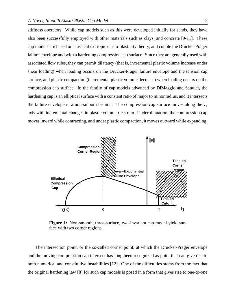
A Novel, Smooth Elasto-Plastic Cap Model 2
stiffness operators. While cap models such as this were developed initially for sands, they have
also been successfully employed with other materials such as clays, and concrete [9-11]. These
cap models are based on classical isotropic elasto-plasticity theory, and couple the Drucker-Prager
failure envelope and with a hardening compression cap surface. Since they are generally used with
associated flow rules, they can permit dilatancy (that is, incremental plastic volume increase under
shear loading) when loading occurs on the Drucker-Prager failure envelope and the tension cap
surface, and plastic compaction (incremental plastic volume decrease) when loading occurs on the
compression cap surface. In the family of cap models advanced by DiMaggio and Sandler, the
hardening cap is an elliptical surface with a constant ratio of major to minor radius, and it intersects
the failure envelope in a non-smooth fashion. The compression cap surface moves along the � 1
axis with incremental changes in plastic volumetric strain. Under dilatation, the compression cap
moves inward while contracting, and under plastic compaction, it moves outward while expanding.
���������������������������������������������������������������������������������������������������������������������
���������������������������������������������������������������������������������������������������������������������������������������������������������������������������
||s||
I1κχ(κ) T
CompressionCorner Region
TensionCornerRegion
EllipticalCompression Cap
Linear−ExponentialFailure Envelope
Tension Cutoff
Figure 1: Non-smooth, three-surface, two-invariant cap model yield sur-face with two corner regions.
The intersection point, or the so-called corner point, at which the Drucker-Prager envelope
and the moving compression cap intersect has long been recognized as point that can give rise to
both numerical and constitutive instabilities [12]. One of the difficulties stems from the fact that
the original hardening law [8] for such cap models is posed in a form that gives rise to one-to-one

A Novel, Smooth Elasto-Plastic Cap Model 3
correspondence between the cap hardening parameter � and the plastic volume strain ��� � in a form
similar to that expressed below in Equation (8). However, if such a one-to-one hardening law is
actually used, then unexpected and perhaps undesired softening behavior may occur when the stress
point is at the compression corner point [13,14]. Motivated by a desire to control and eliminate
unwanted softening behavior at the compression corner point, Sandler and Rubin [13] proposed
a modified discontinuous hardening law which prevented softening material responses. Resende
and Martin [14] subsequently showed, however, that a discontinuous hardening law can lead to an
incomplete model in the sense that there is a region in strain rate space at the compressive singular
corner point which cannot be covered by any possible stress rate. The basic reason for this lack
completeness was traced to the discontinuity of the hardening law at the compression corner.
Using an elegant integration theory for non-smooth multi-surface plasticity [15], based on
closest point projection return mapping algorithms [16] Simo et al. [17] then developed a ro-
bust numerical implementation of the cap model in terms of algorithms for determining yield
activity based on the Kuhn-Tucker conditions. As part of their new implementation, Simo et
al. [17] proposed a modified continuous hardening law which precluded softening and avoided the
completeness issue raised by Resende and Martin [14]. They formulated consistent algorithmic
loading/unloading conditions and closest point projection return mapping algorithms for all possi-
ble modes of yield surface activity. In a subsequent work [18], Hofstetter, Simo and Taylor (1993)
modified the cap model’s hardening law such that it was associated, thus resulting in symmetrical
consistent tangent operators. Nevertheless, even with the vital improvements advanced in [15-18],
problems remain with the non-smooth, three-surface cap model. As will be shown below, one of
the primary remaining difficulties is that the material tangent operators in both the compression
corner and tension corner regions are singular in that they do not provide any bulk/volumetric
material stiffness. This is completely unrealistic, and can lead to difficulties in structural analysis
of soil systems. While there are a number of ad-hoc ways to deal with this singularity of tangent
operators at the corner points (such as the introduction of artificial bulk stiffness in the corner
regions, or resorting to usage of visco-plasticity as proposed in [15] for general non-smoothess),
these approaches are less than satisfactory.
The intent of this manuscript is, therefore, to introduce and fully develop a novel, smooth
cap model wherein the three surfaces (a Drucker-Prager failure envelope; a hardening circular
A Novel, Smooth Elasto-Plastic Cap Model 4
compression cap; and a fixed circular tension cap) intersect in a smooth fashion such that there
are no corner regions. This smoothness therefore precludes many of the historical difficulties
associated with the corner regions including: material softening response, lack of completeness,
and singularity of material tangent operators. The model features essentially the same physical
degree of realism as the preceding cap models, but its numerical performance characteristics
are significantly enhanced. In Section 2 of this manuscript, a non-smooth cap model is briefly
introduced, and the difficulty with singular tangent operators at the corner regions is highlighted.
Section 3 then presents a novel smooth cap model along with a detailed integration algorithm
and expressions for consistent tangent operators. The integration algorithm presented is based
on a Backward Euler integration of the rate constitutive equations, which give rise to an elastic-
predictor, plastic-corrector (return map) stress update algorithm. Differentiation of the incremental
stress update algorithms provides expressions for the so-called consistent tangent operators which
facilitate good convergence characteristics in implicit structural analysis of soil structures. In
Section 4, the excellent performance of the model is first demonstrated on a number of simple
material test type computations, and then on full scale slope stability and bearing capacity type
problems.
2. ASSESSMENT OF A NON-SMOOTH CAP MODEL
2.1 Basic Forms and Rate Equations
For simplicity and clarity, the elastoplastic constitutive equations of a non-smooth three sur-
face cap model are considered here in a small deformation framework. These equations can be
straightforwardly extended to a large-deformation framework as necessary. The small strain tensor
admits the usual additive elastic, plastic decomposition as follows:
� = ��� + � � (1)
where ����� � and � � are the total, elastic, and plastic strain vectors, respectively. The elastic response
of the material is assumed to be characterized by a constant isotropic tensor C =�
1 � 1 + 2 � Idev
such that the incremental stress response of the material is given by:
= C :����� (2)
A Novel, Smooth Elasto-Plastic Cap Model 5
In stress space, the elastic domain is bounded by three distinct yield surfaces which are functions
of the two invariants � 1 = tr( ) and�s�, where s is the deviatoric part of the stress tensor (i.e.
s = Idev : ). The three surfaces comprising the yield surface intersect in a non-smooth manner as
shown in Figure 1.
The mathematical forms of the individual yield functions,���
( � � ) � = 1 � 2 � 3 are:
�1( ) =
����� 2 �� 2� ( � 1) 0 (3)
�2( � � ) =
����� 2 ���� ( � 1� � ) 0 (4)
�3( ) = � 1
�� � 0 (5)
Specific forms for � � and ��� are:
� � ( � 1) = � ��� � 1��� exp ��� � 1 � (6)� � ( � 1
� � ) = � 2� ( � ) ��� � 1� �� � 2 � (7)
where the following are material model constants: ��� 0, � � 0, ��� 0, � � 0, and�
� 0. The
yield surfaces�
1 = 0 and�
3 = 0 depend only on the stress invariants � 1 and�����
, and thus remain
fixed in stress space. In the function � � , the constants � and � are related, respectively, to the
Mohr-Coulomb angle of friction � and cohesion � . The aspect ratio of the elliptical compression
cap is provided by the dimensionless constant�
. The cap is permitted to translate along the � 1
axis, and in particular moves to the right (� � 0) during plastic dilatation of the medium, and to
the left (� � 0) during plastic compaction.
The hardening law for this model derives from the fact that the volumetric crush curve (plastic
volumetric strain � � � versus � 1) is assumed to be an exponential of the form:
� � � = �! � 1 � exp[ "$# ( � )] � (8)
where # ( � ) % � � � � � ( � ) is the apex point of the cap surface on the � 1 axis; � � � denotes the
plastic volumetric strain in the soil (or porous medium) as measured from a virgin completely
unloaded state; represents the maximum possible plastic volumetric strain for the medium, with
the reference state being the material’s virgin unloaded state; and "'& 1 = � ref1 denotes the value
(absolute) of � 1 at which ( & 1 ) 100% of the medium’s original crushable porosity remains, and�
is a
A Novel, Smooth Elasto-Plastic Cap Model 6
dimensionless constant providing the ratio of major to minor radii of the elliptical compression cap
surface. Differentiating Eq. (8) with respect to � allows us to obtain a variable tangent hardening
modulus���
( � ) for � as follows:
� �( � ) =
��� � � � =
exp[ � " # ] "$# � � (9)
where # � = 1 � � � �� ( � ). Based on Eqs. (8) and (9), it is clear that as #�� � then���
( � ) � �and � � � � �! . This nonlinear hardening modulus
���( � ) is used to provide a nonlinear incremental
hardening law governing movement of the cap parameter:
� =� �
( � ) � ( � � ) � (10)
The flow rule for this non-smooth model is associated, and since multiple surfaces are poten-
tially active at any given instant, it takes Koiter’s generalized form:
� � =� � �
�� � � � (11)
The plastic consistency parameters are denoted by ��
( � = 1 � 2 � 3), and their time derivatives are
proportional to the instantaneous magnitudes of the plastic deformation processes at a fixed material
point with respect to each of the three yield functions. Loading and unloading criteria are specified
by the Karesh-Kuhn-Tucker conditions as
� � 0;�� � 0;
�� � �
= 0 (12)
with generalized plastic consistency expressed by
�� � �
= 0 � (13)
In accordance with the KKT conditions, this elasto-plastic constitutive model poses six different
different possibilities:
0. The stress point lies inside of yield surface and� �
� 0, � = 1 � 2 � 3. In thiscase the material response is incrementally elastic;
1. Loading is occuring on surface 1, such that�
1 = 0 and� 1 � 0;
2. Loading is occuring on surface 2, such that�
2 = 0 and� 2 � 0;
3. Loading is occuring on surface 3, such that�
3 = 0 and� 3 � 0;
4. Surfaces 1 and 2 are simultaneously active�
1 =�
2 = 0 and� 1 � 0,
� 2 � 0;
5. Surfaces 1 and 3 are simultaneously active�
1 =�
3 = 0 and� 1 � 0,
� 3 � 0;
In essence, this model is comprised of five elasto-plastic sub-cases as listed above. Those that can
create some difficulty are the corner cases 4 and 5 as briefly detailed below.

A Novel, Smooth Elasto-Plastic Cap Model 7
2.2 The Problem: Singular Tangent Operators at Corner Points
To illustrate the difficulty associated with the corner cases of non-smooth cap models, the return
mapping algorithms for the corner case 4 is briefly formulated below. Upon differentiating the
case 4 stress update algorithm, it is shown that the associated consistent tangent operator obtained is
singular in that it provides no volumetric stiffness for the material. This can lead to singular (rank
deficient) global tangent stiffness matrix operators, and severe computational difficulties when
attempting to solve global force balance finite element equations. While band-aid type remedies to
this problem are available, the difficulty can be avoided altogether by resorting to a cap model in
which the yield surfaces intersect in a smooth fashion. Such a model is introduced in the following
section.
If a Backward Euler integration algorithm is applied to the elastoplastic rate constitutive equa-
tions laid out above, then a stress update algorithm with an elastic predictor and a plastic corrector
(return mapping) is the result. The elastic predictor assumes incrementally elastic behavior, and
leads to a trial stress state as follows:
tr� + � = �� + C :� ���
+1 (14)
� tr�+1 = � � � (15)
If the elastic predictor lies outside of the elastic domain, then one or more of the intersecting yield
surfaces will be active. If it is assumed that the elastic predictor lies in the attractor region for
the corner point at which the compression cap and failure envelope intersect (i.e. the compression
corner region of Figure 1) then the return map (plastic corrector) brings the stress state back to the
indicated corner point. Specifically,
�+1 = tr� + �
� �(� � � � ) � +11 � 2 � � e� � +1 (16)
where (� � � � ) � +1 = � (
� � � �+1) is the plastic volumetric strain increment, and
�e� � +1 = Idev : (
� � � �+1) is
the deviatoric plastic strain increment. The total plastic strain increment associated with the return
map is� � � �
+1 = ˆ� 1�+1
�1 �
+1+ ˆ� 2�
+1
�2 �
+1
� (17)

A Novel, Smooth Elasto-Plastic Cap Model 8
The magnitudes of the plastic deformation proceesses ˆ� 1�+1 and ˆ� 2�
+1 are computed by enforcing
(�
1) � +1 = 0 and (�
2) � +1 = 0, which provides
ˆ� 1�+1 =
� � � ( � tr1 ) � +1
9� ����������
1 � � +1
(18)
ˆ� 2�+1 =
�s � +1
� �� � ( � � )2 �
� � � � ( � tr1 ) � +1
9� � ��������
1 � � +1
� (19)
Hence the return map to the corner point is very simple and involves no iterations.
However, when one differentiates the stress increment produced by this integration algorithm
with respect to the driving strain increment, a singular consistent tangent operator is obtained.
Differentiating Eq. (16) [and the subsidiary terms in Eqs. (17)-(19)] with respect to� � �
+1 provides
the following consistent tangent operator when surfaces 1 and 2 are simultaneously active:
� � �+1� � � �+1
= 2 � � 1 � 2 � ( ˆ� 1�+1 + ˆ� 2�
+1)� �tr�
+1
� � [Idev� n � +1 � n � +1] � (20)
where n � +1 is the deviatoric component of the unit normal to the yield surface at the converged
stress point. Clearly, this tangent material stiffness operator has no bulk stiffness, and thus it is
singular. A similarly singular tangent operator with no bulk stiffness occurs at the corner point
between the tension cutoff surface and the failure envelope.
It is the authors’ experience that such singular material tangent operators can give rise to rank
deficient global tangent stiffness matrices when implicit nonlinear finite element calculations are
performed with non-smooth cap models. There are a number of band-aid type solutions that can
be employed to deal with this problem. Two in particular are:
i introduction of an artificial (and small) bulk stiffness to the material tangent defined inEquation (20); and
ii introduction of visco-plasticity to the model, which allows the tangent operators in cornerregions to remain non-singular as long as the inviscid limit is not approached.
Neither of these band-aid type approaches deal with the root cause of the problem, however, which is
the existence of corner points on the yield surface. Furthermore, the introduction of the artificial bulk
stiffness in the corner regions can lead to a tangent operator that is inconsistent with the stress update
algorithm, and thus result in slow convergence behavior in solving nonlinear global force balance
equations. The introduction of viscoplastic behaviors to avoid singularity of tangent operators in
A Novel, Smooth Elasto-Plastic Cap Model 9
the corner regions makes the structural analysis problem somewhat more involved, since for each
structural load increment applied, a number of time steps must be permitted to compute the time-
dependent deformation response of the structure. Furthermore, the rate dependence introduced
with viscoplasticity can obscure more physically based rate effects such as those associated with
pore pressure diffusion phenomena. A more fundamental approach to this problem of singular
tangent operators in corner regions is therefore proposed below, with the introduction of a smooth
cap model having no corner regions.
3. INTRODUCTION OF A NOVEL, SMOOTH CAP MODEL
3.1 Basic Forms and Rate Equations
To deal with the difficulties associated with a non-smooth yield surface, a yield surface (Fig-
ure 2) made up of three smoothly intersecting yield functions is introduced here. The form of the
three yield functions,� �
( � � )( � = 1 � 2 � 3) are specified in terms of functions � � � � � and � � which
are respectively called the Drucker-Prager envelope function, the compression cap function, and
the tension cap function:
�1( ��� ) =
��� � �� � ( � 1) 0 (21)
�2( ��� � � ) =
��� � 2 ���� ( � 1� � ) 0 (22)
�3( ��� ) =
��� � 2 �� � ( � 1) 0 � (23)
where�
= s ��� and��� �
= [�
:�
]12 . As is customary, s denotes the deviatoric stress, and � denotes
a purely deviatoric back stress associated with kinematic hardening.
The specific forms of � � � � � and � � differ somewhat from the forms introduced previously in
concert with the non-smooth cap model and are defined here as
� � ( � 1) = � + ��� 1 � exp( � � 1) ��1 ( � ) � 1 � �1 (24)� � ( � 1� � ) =
� 2( � ) � ( � 1� � )2 � 1 � � 1 ( � ) (25)� � ( � 1) =
� 2� � � 12 � 1 � � �1 � (26)
A Novel, Smooth Elasto-Plastic Cap Model 10
||η||
I1κχ(κ)
Translating,Circula rCompressionCap
Exponential Drucke r−PragerFailure Envelope
CircularTension Cap
TIC1(κ) IT1
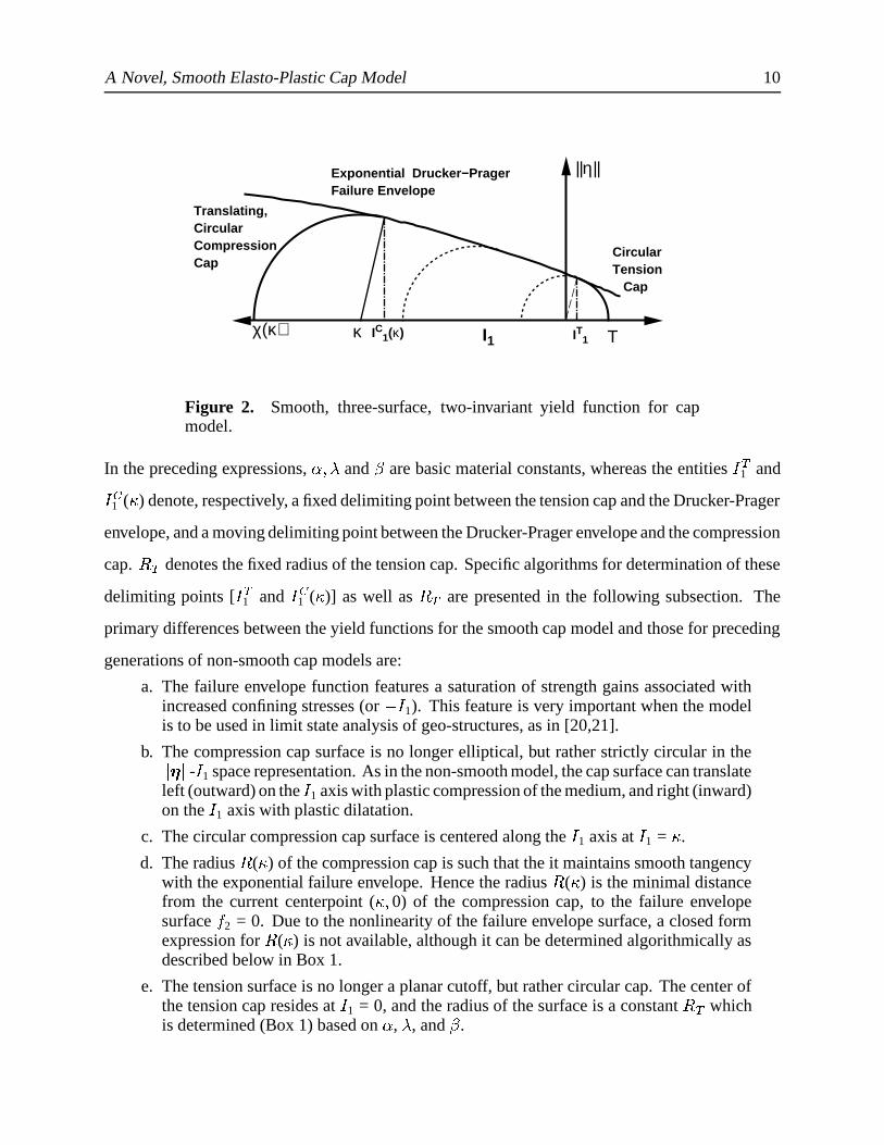
Figure 2. Smooth, three-surface, two-invariant yield function for capmodel.
In the preceding expressions, � � � and � are basic material constants, whereas the entities � �1 and
� 1 ( � ) denote, respectively, a fixed delimiting point between the tension cap and the Drucker-Prager
envelope, and a moving delimiting point between the Drucker-Prager envelope and the compression
cap.�� denotes the fixed radius of the tension cap. Specific algorithms for determination of these
delimiting points [ � �1 and � 1 ( � )] as well as�� are presented in the following subsection. The
primary differences between the yield functions for the smooth cap model and those for preceding
generations of non-smooth cap models are:
a. The failure envelope function features a saturation of strength gains associated withincreased confining stresses (or � � 1). This feature is very important when the modelis to be used in limit state analysis of geo-structures, as in [20,21].
b. The compression cap surface is no longer elliptical, but rather strictly circular in the��� �- � 1 space representation. As in the non-smooth model, the cap surface can translate
left (outward) on the � 1 axis with plastic compression of the medium, and right (inward)on the � 1 axis with plastic dilatation.
c. The circular compression cap surface is centered along the � 1 axis at � 1 = � .
d. The radius�
( � ) of the compression cap is such that the it maintains smooth tangencywith the exponential failure envelope. Hence the radius
�( � ) is the minimal distance
from the current centerpoint ( � � 0) of the compression cap, to the failure envelopesurface
�2 = 0. Due to the nonlinearity of the failure envelope surface, a closed form
expression for�
( � ) is not available, although it can be determined algorithmically asdescribed below in Box 1.
e. The tension surface is no longer a planar cutoff, but rather circular cap. The center ofthe tension cap resides at � 1 = 0, and the radius of the surface is a constant
�� which
is determined (Box 1) based on � , � , and � .

A Novel, Smooth Elasto-Plastic Cap Model 11
f. The model features kinematic hardening which permits the elastic domain to translateabout hydrostatic stress axis.
Since the Mohr-Coulomb yield criterion has a long history of usage in classical soil mechanics,
geotechnical engineers often think of soil shear strength characteristics in terms of the Mohr-
Coulomb cohesion � and friction angle � . Here, the nonlinear Drucker-Prager failure envelope
with tension and compression caps, and with saturating frictional effects is employed since:
1. It captures the saturation of soil strength with increasing effective confining stresses;and
2. It is a completely smooth model having no corner regions. The Drucker-Pragermodel does not suffer from the non-smooth corner regions that generally afflict Mohr-Coulomb type soil models [22].
So that the results of the present work can be placed in context and even compared with results from
classical geotechnical analysis methods wherein the Mohr-Coulomb failure criterion is routinely
considered, the failure envelope in Equations (21) and (24) is re-written by taking its Taylor series
expansion about � 1 = 0:
�1(�
) =��� � � � � ��� � 1
� 1 +� � 1
2+
( � � 1)2
6+
( � � 1)3
24+ � � � ��� (27)
where � �= � � is the slope of the envelope at � 1 = 0. For small values of � 1 (i.e. � � 1 � � 1), the
linearized form of the yield function is:
�1(�
)�=��� � � � � ��� � 1 � (28)
which is simply a variation of the linear Drucker-Prager yield criterion. A correspondence can
be established between the two parameters � and � of the linearized Drucker-Prager envelope
of Equation (28) and the cohesion � and friction angle � of the Mohr-Coulomb envelope. For
example, translations from Mohr-Coulomb parameters to linear Drucker-Prager parameters have
been provided by Chen and Saleeb (1982) as:
� = � 2 ��1 + 4
3 tan2 � � 12
� = � 2 tan �3�1 + 4
3 tan2 � � 12
� (29)
These equations can be inverted to provide a translation from linear Drucker-Prager envelope
parameters to Mohr-Coulomb which will be used in the following section.
� =�� 2 � 1 +
43
tan2 ��� 12
tan � =3� 2� �
1 � 6 � 2 � & 12 � (30)

A Novel, Smooth Elasto-Plastic Cap Model 12
The flow rule for this model is associated, and thus
� � =�
�� � � � � (31)
While this generalized form of the flow rule would appear to imply that more than one yield function
can be active at a given instant, this will not occur with this model due to the smoothness of the
yield surface of the cap model. The Karesh-Kuhn-Tucker loading/unloading conditions and the
plastic consistency conditions for the smooth model are expressed in a manner identical to that for
the non-smooth cap model in Equations (12) and (13). In rate form, the non-associated hardening
law for the cap parameter � is identical to that used for the non-smooth cap model, specifically:
� =� �
( � ) � ( � � ) (32)
where���
( � ) is the tangent hardening modulus for the cap parameter which is still given by
� �( � ) =
( ��� [ � "$# ( � )] "$# � ( � )(33)
where " and are material parameters which retain the same meaning as they have in the non-
smooth cap model. The maximum value the cap parameter � can take is limited to 0, such that
� = min � 0 � � � . The parameter # ( � ) still defines the intersection of the cap with hydrostatic stress
axis as a function of the hardening parameter, � as # ( � ) = � � �( � ) � A purely deviatoric linear
kinematic hardening law is employed with this model, the rate form of which is
� = � Idev) � � (34)
where H is a constant plastic hardening modulus.
3.2 Determination of Compression Cap Radius
With the non-smooth cap model, the minor radius of the elliptical compression cap surface can
be determined in closed form simply as � � ( � ). In the present model, however, the radius of the
circular compression cap is determined such that when the cap is centered at ( � 1 = � � � � � = 0),
the cap surface smoothly intersects with the exponential Drucker-Prager envelope. For a linear
Drucker-Prager failure envelope, expressions are available for the cap surface radius as a function of
A Novel, Smooth Elasto-Plastic Cap Model 13
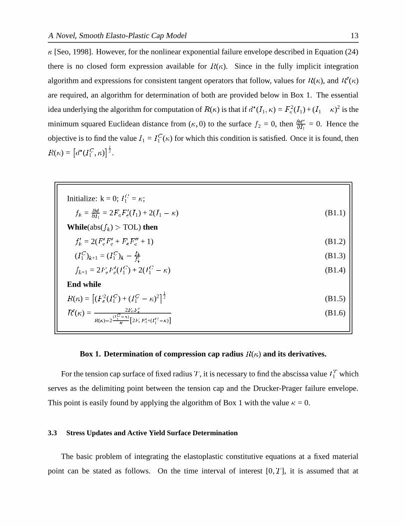
� [Seo, 1998]. However, for the nonlinear exponential failure envelope described in Equation (24)
there is no closed form expression available for�
( � ). Since in the fully implicit integration
algorithm and expressions for consistent tangent operators that follow, values for�
( � ), and� �
( � )
are required, an algorithm for determination of both are provided below in Box 1. The essential
idea underlying the algorithm for computation of�
( � ) is that if� �
( � 1� � ) = � 2� ( � 1) + ( � 1
� � )2 is the
minimum squared Euclidean distance from ( � � 0) to the surface�
2 = 0, then��������
1= 0. Hence the
objective is to find the value � 1 = � 1 ( � ) for which this condition is satisfied. Once it is found, then�
( � ) = � � � ( � 1 � � ) 12 .
Initialize: k = 0; � 1 = � ;���
=������
1= 2 � � � �� ( � 1) + 2( � 1
� � ) (B1.1)
While(abs(� �
) � TOL) then� ��
= 2( � �� � �� + � � � � �� + 1) (B1.2)
( � 1 )�
+1 = ( � 1 )� ���� � (B1.3)
� �+1 = 2 � � � �� ( � 1 ) + 2( � 1 � � ) (B1.4)
End while�
( � ) = � ( � 2� ( � 1 ) + ( � 1 � � )2 12 (B1.5)
� �( � ) = 2
��� � ���
( � ) & 2( ���
1 ��� )� [2� � � �� +(
� �1 & � )]
(B1.6)
Box 1. Determination of compression cap radius�
( � ) and its derivatives.
For the tension cap surface of fixed radius , it is necessary to find the abscissa value � �1 which
serves as the delimiting point between the tension cap and the Drucker-Prager failure envelope.
This point is easily found by applying the algorithm of Box 1 with the value � = 0.
3.3 Stress Updates and Active Yield Surface Determination
The basic problem of integrating the elastoplastic constitutive equations at a fixed material
point can be stated as follows. On the time interval of interest [0 � ], it is assumed that at

A Novel, Smooth Elasto-Plastic Cap Model 14
time � � � [0 � ] the total and plastic strain tensors are known as are the stress and hardening
variables: that is � � � � � � � � � � � � � � � � are known at time � � � The incremental strain� � �
+1 over
a given time step [ � � � � � +1], is assumed to be provided, and the remaining independent variables� � � � +1� �
+1� � � +1
��� �+1 � must be updated by the integration of the rate constitutive equations. This
is accomplished here using well-established operator-splitting, elastic-predictor, plastic-corrector
methods. Briefly, the updated stress can be written as follows:
�+1 = � + C :
� � ��+1 = � + C :
� � �+1� C :
� � � �+1� (35)
In accordance with the operator-split, a given strain increment� � �
+1 is first assumed to result in an
incremental material response which is fully elastic, leading to a the so-called incrementally elastic
trial stress predictor computed as
tr� + � = � + C :� � �
+1 (36 � )
= �� +� � �
��
+11 + 2 � � e � +1 (36 � )
where� �
��
+1 is the incremental volumetric strain, and�
e � +1 is the incremental deviatoric strain.
Taking the trace and deviatoric parts of the elastic trial stress leads to:
( � 1)����
+1 = ( � 1) � + 9� � �
��
+1 (37 � )
s����
+1 = s � + 2 � Idev� � �
+1� (37 � )
Also, the trial value of the cap hardening parameter � and the back stress � remain unchanged
during the elastic predictor so that � tr�+1 = � � and � ����
+1 = � � . The trial yield function values
(�
1)tr�+1, (
�2)tr�
+1, (�
3)tr�+1 are then computed based on the trial stress and hardening parameters. If
(�
1)tr�+1 � TOL1 or (
�2)tr�
+1 � TOL2 or (�
3)tr�+1 � TOL3 then the predicted elastic trial state lies
outside of the elastic domain, and a plastic correction must be performed.
The manner in which the plastic correction is computed depends upon which one of the yield
constraints is in fact active. For the general case of non-smooth plasticity models, determination
of the so-called active set of yield contraints can be a challenging task as demonstrated by Simo
et al [55]. Even for this smooth plasticity model, great caution is needed in determining which,
if any, of the three yield constraints will be active at any given instant. The algorithm used for

A Novel, Smooth Elasto-Plastic Cap Model 15
determining yield function activity with the proposed smooth cap model is shown in Box 2. The
underlying concept for the algorithm of Box 2 is that since the Drucker-Prager surface envelopes
both the tension and compression cap surfaces, when it is violated , then the second and third yield
criteria will necessarily be violated as well. Thus, when (�
1)tr�+1 � TOL1, any of the three yield
surfaces could in fact be active. Ultimately, however, only one will indeed be active. Due to the
smoothness of the yield surface and the nonlinearity of the hardening law for � there is no simple
a priori criterion for determining which of the three yield constraints will be active based on the
elastic trial stress state.
Since a determination of active yield constraints is not possible from the trial stress, a determi-
nation of activity must be determined from updated stress states. Consequently, the closest point
projection return map of the elastic trial stress to the Drucker-Prager surface is performed and an
update of � consistent with the return map is performed (leading to a value denoted by � case1�+1 ). If the
returned stress point lies in the updated domain of the Drucker-Prager surface, then that constraint
will indeed be active. However, if the return point should lie in the updated domain of either
the compression cap or the tension cap, they would represent the active constraint. These ideas
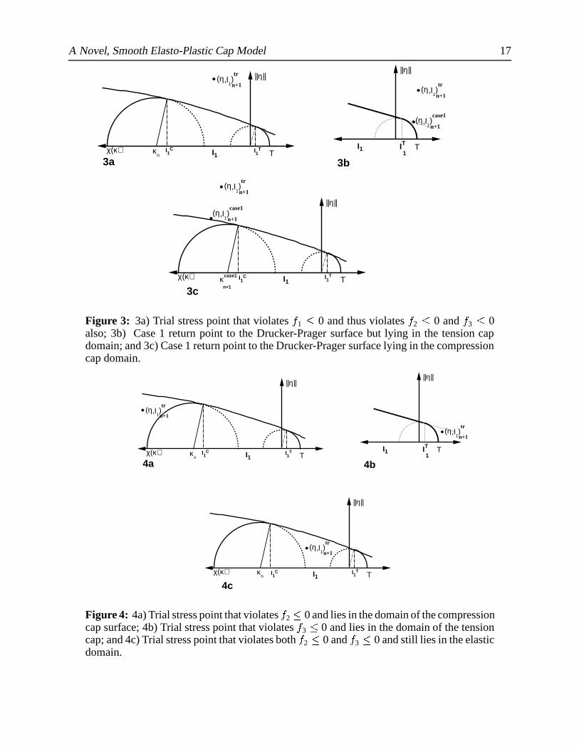
are demonstrated graphically in Figure 3. Referring specifically to Figure 3b, if ( � 1)case1�+1 � � �1 ,
then the return point lies in the domain of the tension cap surface, and so the tension cap surface
will be active which means that the return map must be re-computed using the Case 3 integration
algorithm. Alternatively, once � 1 ( � case1�+1 ) is computed (Box 1), and if ( � 1)case1�
+1 � � 1 ( � case1�+1 ), then
the compression cap is active and the return map must be re-computed using the Case 2 integration
algorithm.
It should be further noted, corresponding to Figure 4, that it is possible for the elastic trial
stress state tr� + � to violate either or both of�
2 0 and�
3 0 but not violate�
1 0. In this case,
it must be determined whether Case 2 or Case 3 is active. A criterion based on the location of
the trial stress point’s value of ( � tr1 ) � +1 with respect to � �1 and � 1 ( � � ) is also provided in the Box 2
algorithm.
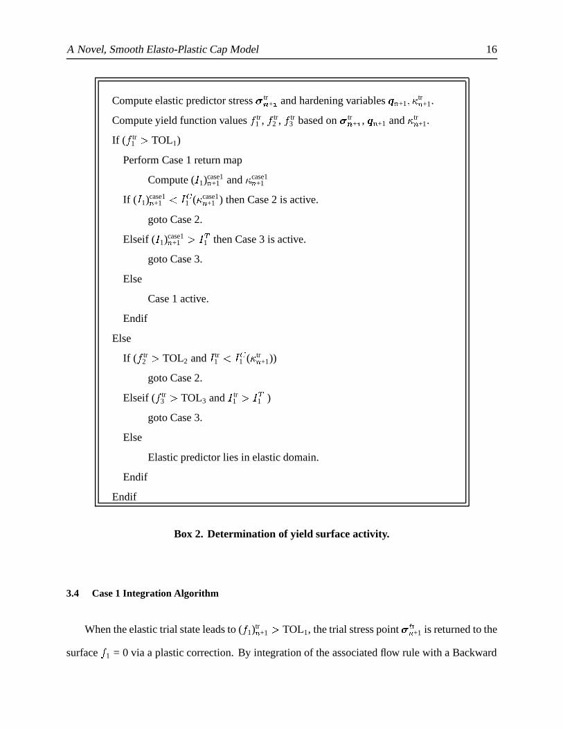
A Novel, Smooth Elasto-Plastic Cap Model 16
Compute elastic predictor stress tr� + � and hardening variables � � +1� � tr�
+1.
Compute yield function values� tr
1 ,� tr
2 ,� tr
3 based on tr� + � ,� �
+1 and � tr�+1.
If (� tr
1 � TOL1)
Perform Case 1 return map
Compute ( � 1)case1�+1 and � case1�
+1
If ( � 1)case1�+1 � � 1 ( � case1�
+1 ) then Case 2 is active.
goto Case 2.
Elseif ( � 1)case1�+1 � � �1 then Case 3 is active.
goto Case 3.
Else
Case 1 active.
Endif
Else
If (� tr
2 � TOL2 and � tr1 � � 1 ( � tr�
+1))
goto Case 2.
Elseif (� tr
3 � TOL3 and � tr1 � � �1 )
goto Case 3.
Else
Elastic predictor lies in elastic domain.
Endif
Endif
Box 2. Determination of yield surface activity.
3.4 Case 1 Integration Algorithm
When the elastic trial state leads to (�
1)tr�+1 � TOL1, the trial stress point
����+1 is returned to the
surface�
1 = 0 via a plastic correction. By integration of the associated flow rule with a Backward
A Novel, Smooth Elasto-Plastic Cap Model 17
(η,I1)tr
n+1
||η||
I1χ(κ) TI1C I1
T
(η,I1)tr
n+1
||η||
I1 TIT
1
3a 3b
κcase1
n+13c
||η||
I1κn
χ(κ) TI1C I1
T
(η,I1)case1
n+1
(η,I1)tr
n+1
(η,I1)case1
n+1
Figure 3: 3a) Trial stress point that violates�
1 0 and thus violates�
2 0 and�
3 0also; 3b) Case 1 return point to the Drucker-Prager surface but lying in the tension capdomain; and 3c) Case 1 return point to the Drucker-Prager surface lying in the compressioncap domain.
||η||
I1χ(κ) TI1C I1
T
||η||
I1 TIT
1
4a 4b
4c
||η||
I1κn
χ(κ) TI1C I1
T
(η,I1)tr
n+1
(η,I1)tr
n+1
(η,I1)tr
n+1
κn
Figure 4: 4a) Trial stress point that violates�
2 0 and lies in the domain of the compressioncap surface; 4b) Trial stress point that violates
�3 0 and lies in the domain of the tension
cap; and 4c) Trial stress point that violates both�
2 0 and�
3 0 and still lies in the elasticdomain.
A Novel, Smooth Elasto-Plastic Cap Model 18
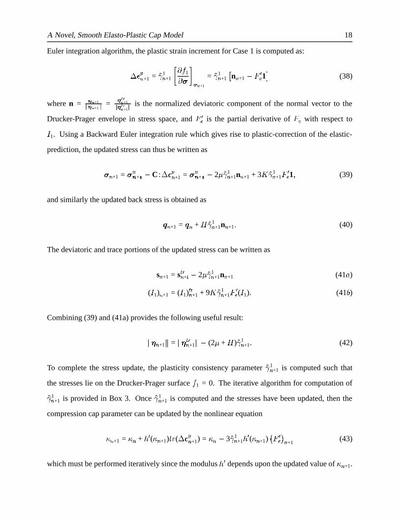
Euler integration algorithm, the plastic strain increment for Case 1 is computed as:
� � � �+1 = ˆ� 1�
+1� �
1 ����
+1
= ˆ� 1�+1� n � +1
�� �� 1 (38)
where n =� �
+1� � �+1� =
������+1� ������+1
� is the normalized deviatoric component of the normal vector to the
Drucker-Prager envelope in stress space, and � �� is the partial derivative of � � with respect to
� 1. Using a Backward Euler integration rule which gives rise to plastic-correction of the elastic-
prediction, the updated stress can thus be written as
��+1 = tr� + �
� C :� � � �
+1 = tr� + �� 2 � ˆ� 1�
+1n � +1 + 3�
ˆ� 1�+1� �� 1 � (39)
and similarly the updated back stress is obtained as
� �+1 = � � + � ˆ� 1�
+1n � +1� (40)
The deviatoric and trace portions of the updated stress can be written as
s � +1 = s����
+� � 2 � ˆ� 1�
+1n � +1 (41 � )
( � 1) � +1 = ( � 1)����
+1 + 9�
ˆ� 1�+1� �� ( � 1) � (41 � )
Combining (39) and (41a) provides the following useful result:
� � �+1�
=��� ����
+1
� � (2 � + � ) ˆ� 1�+1� (42)
To complete the stress update, the plasticity consistency parameter ˆ� 1�+1 is computed such that
the stresses lie on the Drucker-Prager surface�
1 = 0. The iterative algorithm for computation of
ˆ� 1�+1 is provided in Box 3. Once ˆ� 1�
+1 is computed and the stresses have been updated, then the
compression cap parameter can be updated by the nonlinear equation
� � +1 = � � +� �
( � � +1) � (� � � �
+1) = � � � 3ˆ� 1�+1� �
( � � +1)� � �� � � +1
(43)
which must be performed iteratively since the modulus���
depends upon the updated value of � � +1.
A Novel, Smooth Elasto-Plastic Cap Model 19
Initialize: k = 0; ( ˆ� 1�+1)
�= 0; ( � 1�
+1)�
= ( � 1�+1)���
;��� �
+1� �
=��� ����
+1
�(
�1)�
=��� �
+1� � ��� � (( � 1�
+1)�) (B3.1)
While (abs( (�
1)�
) � TOL) then� �(� 1�
+1)���1 � � = 9 � � ��
1 & 9 � ˆ� 1�
+1
� � �� (B3.2)
(�
1)� �
= � (2 � + � ) ��� �� � �(� 1�
+1)���1 � � (B3.3)
( ˆ� 1�+1)
�+1 = (ˆ� 1�
+1)� � ( � 1)
( � �1) (B3.4)��� �+1
� �+1 =
��� ����+1
� � (2 � + � )( ˆ� 1�+1)
�+1 (B3.5)
update ( � 1�+1)
�+1 such that ( � 1�
+1)�
+1� ( � 1�
+1)��� � 9
�( ˆ� 1�
+1)�
+1� �� (( � 1�
+1)�
+1) = 0 (B3.6)
(�
1)�
+1 =��� �
+1� �
+1�� � (( � 1�
+1)�
+1) (B3.7)
k = k + 1
End while
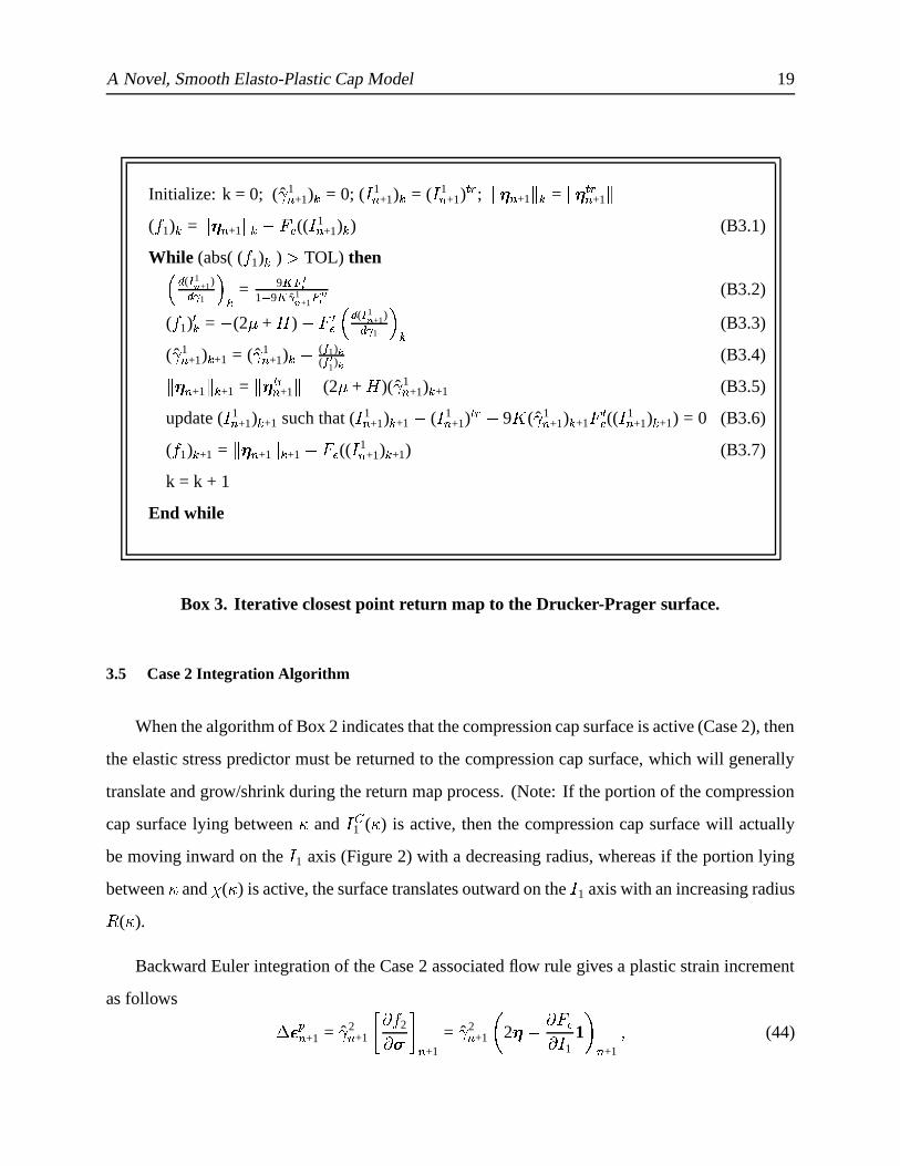
Box 3. Iterative closest point return map to the Drucker-Prager surface.
3.5 Case 2 Integration Algorithm
When the algorithm of Box 2 indicates that the compression cap surface is active (Case 2), then
the elastic stress predictor must be returned to the compression cap surface, which will generally
translate and grow/shrink during the return map process. (Note: If the portion of the compression
cap surface lying between � and � 1 ( � ) is active, then the compression cap surface will actually
be moving inward on the � 1 axis (Figure 2) with a decreasing radius, whereas if the portion lying
between � and # ( � ) is active, the surface translates outward on the � 1 axis with an increasing radius�
( � ).
Backward Euler integration of the Case 2 associated flow rule gives a plastic strain increment
as follows� � � �
+1 = ˆ� 2�+1� �
2 � �+1
= ˆ� 2�+1 � 2
� � � � � 1
1 � �+1
� (44)
A Novel, Smooth Elasto-Plastic Cap Model 20
resulting in the following stress update equation:
��+1 = tr� + � + 3
�ˆ� 2�
+11 � � � � 1� �
+1
� 4 � ˆ� 2�+1s � +1
� (45)
Decomposing the updated stress into its deviatoric and bulk components provides:
s � +1 = s����
+1� 4 � ˆ� 2�
+1
� �+1 (46 � )
( � 1) � +1 = ( � 1)tr�+1 + 9
�ˆ� 2�
+1 � � � � 1� �
+1
� (46 � )
Similarly, the compression cap parameter � and the back stress � have updates of the form:
� � +1 = � � � 3� �
( � � +1) ˆ� 2�+1 � � � � 1
� �+1
(47 � )
� �+1 = � � + 2 � ˆ� 2�
+1
� �+1� (47 � )
Taking the difference between Eqs. (46a) and (47b) yields the following useful results:
� �+1 =
� ����+1� 1 + 2(2 � + � ) ˆ� 2�
+1 ��� �
+1�
=
��� ����+1
�� 1 + 2(2 � + � ) ˆ� 2�
+1 � (48)
The objective of the plastic correction stress update algorithm for Case 2 is thus to solve for
the value of the generalized plastic consistency parameter ˆ� 2�+1, as well as � 1 and � , which satisfy
Equations (46b), (47a) and the plastic consistency condition, namely,
�2�
+1 =
� � ����+1
� 2� 1 + 2(2 � +
�) ˆ� 2�
+1 2��� � ( � 1
�+1� � � +1) = 0 � (49)
Hence, the Case 2 return map involves solving a system of three highly nonlinear equations [(46b),
(47a) and (49)] for the three coupled parameters ˆ� 2�+1, ( � 1) � +1 and � � +1. So that a solution to this
system of equations can be reliably obtained, a robust and fully implicit algorithm is developed
below.
Since a sequential linearization algorithm is used to solve the system, the total derivative of�
2
with respect to ˆ� 2�+1 is needed, and is thus computed as
� �2�
ˆ� 2�+1
=
� ��� �+1� 2
�ˆ� 2�
+1
� � � � � 1� �
� 1�ˆ� 2�
+1
� � � � � � ���
ˆ� 2�+1
(50)
where the first term on the right is easily evaluated as:� ��� �
+1
� 2�
ˆ� 2�+1
=� 4(2 � + � )
��� �+1
� 2� 1 + 2(2 � + � ) ˆ� 2�
+1 � (51)

A Novel, Smooth Elasto-Plastic Cap Model 21
Since the derivatives of ( � 1) � +1 and � � +1 are coupled, they must be written as follows:���11
�12�
21�
22 � � � �1�
ˆ� 2�
+1� ��ˆ� 2�
+1 � =
� �1�2 � (52)
where:
A = �� 1 � 9�
ˆ� 2�+1
� � 2 ���� � 21 � � 9
�ˆ� 2�
+1
� � 2 ���� �1� � �
3� �
ˆ� 2�+1
� � 2 � �� � 21 � 1 + 3ˆ� 2�
+1
� � � � � ��� ����1 � +
� � � � 2 � ����1� � � �� (53 � )
and
F = � 9� � ��������
1 �� 3� � � � � ����
1 � � � (49 � )
Utilizing Cramer’s Rule, the desired derivatives can be straightforwardly obtained as follows:
�� 1�
ˆ� 2�+1
=( � 1
�22��
2
�12)
(�
11�
22� �
12�
21)(54 � )
���
ˆ� 2�+1
=( � 2
�11��
1
�21)
(�
11�
22� �
12�
21)(54 � )
With all the preceding derivatives in hand, the fully implicit closest point projection algorithm for
determination of ˆ� 2�+1 is shown in Box 4.
Once a trial value of ˆ� 2�+1 is obtained (in the algorithm of Box 4), then � 1 and � must be
updated. Due to the nonlinearity of the update Equations (46b) and (47a), the update of � 1 and �
is nontrivial, even with a fixed value of ˆ� 2�+1. Defining a residual vector based on Eqs. (46b) and
(47a) as follows,
r( � 1� � ) = � ( � 1) � +1
� ( � 1)����
+1� 9
�ˆ� 2�
+1
� � ������1 �
� � � � + 3� �
( � � + 1)ˆ� 2�+1
��� ������1 � � (55)
a Newton’s method based on iterative linearization of the residual function is presented in Box 5
for updating � 1 and � .

A Novel, Smooth Elasto-Plastic Cap Model 22
�= 0
( � 1)��
+1 = ( � 1)����
+1� �
��
+1 = �����
+1� � ��
+1 =� ����
+1
compute� �
2 =� tr
2 =�
2(� ����
+1� ( � 1)
����+1� � tr�
+1)
While (� �
2 � TOL2) then
compute� � � 2�
ˆ� 2 �
�+1
�+1
by Eqs. (50), (51), (54)
( ˆ� 2)�
+1�+1 = (ˆ� 2)
��
+1� � �
2
� � � 2�ˆ� 2 � & 1� (B4.1)
update� � �
+1
� � +1 by Eq. (48)
iteratively update ( � 1)�
+1�+1 and �
�+1�+1 (see Box 5)
compute (�
2)�
+1�+1 by Eq. (49)�
=�
+ 1
End while
given ˆ� 2�+1, ( � 1) � +1, � � +1, update stresses and compute tangent operator
return
Box 4. Fully Implicit Return Map Algorithm for CASE 2.

A Novel, Smooth Elasto-Plastic Cap Model 23
for notational simplicity, let � 1 = � 1 and �2 = �
�= 0
let ���1 = ( � 1)� � +1 and ���2 = � � � +1 assume prior values (see Box 4)
compute r(x� ) by Eq. (55)
While�r(x� )
�� TOL) then
x� +1 = x� � � � r�x & 1
�) r� (B5.1)
update r(x� +1) by Eq. (55)�
=�
+ 1
End while
Box 5. Algorithm for Simultaneous Update of � 1 and � for CASE 2.
Remark 1: For each iteration cycle of the algorithm in Box 4, once ˆ� 2 is updated, exactupdates of both � 1 and � are coupled and nonlinear, requiring a sub-iteration loop.
3.6 Case 3 Integration Algorithm
When the algorithm of Box 2 indicates that the tension cap surface is active (Case 3), or when
the return point for Case 2 lies in the domain of the tension cap, then the stress must be returned
to the tension cap surface. Since the tension cap has a fixed radius, the Case 3 return mapping
algorithm is considerably simpler than that for the compression cap (Case 2).
Integration of the associated Case 3 flow rule gives the following plastic strain increment,
� � � �+1 = ˆ� 3�
+1� �
3 � �+1
= ˆ� 3�+1 � 2
� � � � � 1
1 � �+1
� (56)
and the corrected stress and back stress can be written as
��+1 = tr� + � + 3
�ˆ� 3�
+11 � � � � 1� �
+1
� 4 � ˆ� 3�+1
� �+1 (57 � )
� �+1 = � � + 2 � ˆ� 3�
+1
� �+1 (57 � )
A Novel, Smooth Elasto-Plastic Cap Model 24
Decomposition of the corrected stresses and back stresses into deviatoric and bulk components
gives
� �+1 =
� ����+1
1 + 2(2 � + � ) ˆ� 3�+1
(58 � )
( � 1) � +1 = ( � 1)tr�+1 + 9
�ˆ� 3�
+1 � � � � 1� �
+1
= ( � 1)tr�+1� 18
�ˆ� 3�
+1 ��
+11
� (58 � )
=( � 1)tr�
+1
1 + 18�
ˆ� 3�+1
The remaining objective of the return map algorithm is to enforce the plastic consistency condition
(�
3) � +1 =
� � ����+1
� 2� 1 + 2(2 � + � ) ˆ� 3�
+1 2�� � ( � 1
�+1) = 0 � (59)
The return map algorithm for Case 3 is necessarily iterative, and the Newton’s Method algorithm
of Box 3 is very efficient and robust. Once the Case 3 return map is successfully completed, the
compression cap parameter � is updated iteratively following Equation (47).
�= 0
( � 1)��
+1 = ( � 1)����
+1� � ��
+1 =� ����
+1
compute (�
3)��
+1 = (�
3)tr�+1 =
�3(� ����
+1� ( � 1)
����+1)
While ((�
3)��
+1 � TOL3) then
compute� � � 3�
ˆ� 3 �
��
+1=
� & 4(2 � + � )� � � 2
1+2(2 � + � ) ˆ� 3� 9 � (
� �� )2
1 & 9 � � � �� ˆ� 3 �
��
+1(B6.1)
( ˆ� 3)�
+1�+1 = (ˆ� 3)
��
+1� � �
3
� � � 3�ˆ� 3 � & 1 � ��
+1
(B6.2)
update� � � +1�
+1
�by Eq. (58a)
update ( � 1)�
+1�+1 by Eq. (58b)
compute (�
3)�
+1�+1 by Eq. (59)�
=�
+ 1
End while
perform update final update of � +1� � �
+1� � � +1, compute tangent operator
return
Box 6. Return Map Algorithm for CASE 3.

A Novel, Smooth Elasto-Plastic Cap Model 25
3.7 Consistent Tangent Operators
In modern computational plasticity, it is now recognized [19] that in order to achieve the
asymptotically quadratic rate of force-balance convergence that is theoretically possible with global
Newton-Raphson force balance iterations, material tangent operators that are consistent with the
implemented (discrete) form of the constitutive models must be utilized. This leads to so-called
consistent tangent operators which generally differ quite significantly from the continuum elasto-
plastic tangent moduli which can be derived from the rate form of the constitutive equations and the
plastic consistency condition. Since the derivation of expressions for consistent tangent operators
is conceptually straightforward [19], albeit algebraically complex, expressions for the consistent
tangent operators for the three subcases of the smooth cap model are presented in the following
sub-sections.
3.7.1 Case 1 Consistent Tangent Operator
The symmetrical Case 1 consistent tangent operator is computed as follows:
C�� ����+1 = Celastic � �
2 � n � +1� �
3 � ��� �1 & 9 � ˆ
� 1�+1
� � �� � 1 � ��2 � n � +1
� �3 � ��� �
1 & 9 � ˆ� 1�
+1
� � �� � 1 ��(2 � + � ) + 9 � (
� �� )2
1 & 9 � ˆ� 1�
+1
� � �� � (60)
+9� 2 ˆ� 1�
+1� � ��
1 � 9�
ˆ� 1�+1� � �� 1 � 1 � 4 � 2 ˆ� 1�
+1��� ����+1
� [I � � � � n � +1 � n � +1]
3.7.2 Case 2 Consistent Tangent Operator
The Case 2 consistent tangent operator is computed as follows:
C�� ����+1 = Celastic � �
5 (1 � � �+1) � �
6 (� �
+1 � 1) +�
7 (1 � 1) � �8 (� �
+1 � � �+1) � �
9Idev (61)
where �1 = 1 � 9
�ˆ� 2�
+1 � 2 � � � 2
1� +
27� � �
( ˆ� 2�+1)2
� � 2 � ���� 21 � � � 2 � ����
1� � �
1 + 3ˆ� 2�+1
� � � � ����������1 � +
� � � � 2 ������1� � ��� (62 � )�
2 =
� 3ˆ� 2�+1� � � � 2 ������ 2
1 �1 + 3ˆ� 2�
+1
� � � � � ��� ����1 � +
� � � � 2 � ����1� � ��� (62 � )
A Novel, Smooth Elasto-Plastic Cap Model 26�3 =
� � 2 ������ 21 � +
�2
� � 2 ������1� � ��
1(62 � )�
4 = � 2 � � � 2
1� �
� 1�ˆ� 2�
+1+ � 2 � �
� 1 � � �
��
ˆ� 2�+1
(62�)�
5 =12
� �� 1 + 2(2 � + � ) ˆ� 2�+1 � � 2�
ˆ� 2�
+1� � � � � 1
� +�
4 ˆ� 2�+1 � (62 ( )�
6 =12
� �� 1 + 2(2 � + � ) ˆ� 2�+1 � � 2�
ˆ� 2�
+1� � � � � 1
� 1�1
+
�2�1 � ��� � � � (62
�)�
7 = 9� 2
� �3 ˆ� 2�
+1 +
��� ��������1 � +
�4 ˆ� 2�
+1 � ��� � ������1 � 1�
1+
�2�1
� ������ � ���� � 2�ˆ� 2�
+1 � (62 � )�8 =
16 � 2
� � 2�ˆ� 2�
+1
� 1 + 4(2 � + � ) ˆ� 2�+1
(1 + 2(2 � + � ) ˆ� 2�+1)2� (62
�)�
9 =8 � 2 ˆ� 2�
+1
1 + 2(2 � + � ) ˆ� 2�+1
(62 � )
Inspection of the above consistent tangent operator proves it to be non-symmetrical arising from
the terms with coeficients�
5 and�
6. This is to be expected, since the hardening law governing the
cap parameter � is non-associated, and the Principle of Maximum Plastic Dissipation guarantees a
symmetric consistent tangent only for associated flow rules and associated hardening laws. [Simo
and Hughes, 1998] Hofstetter et al [18] developed an associated hardening law for the cap parameter
� and found that this did indeed lead to a symmetrical expression for the Case 2 consistent tangent
operator. However, implementing an associated hardening law for � changes the mechanical
response characteristics of the model. Specifically, in the implementation presented in [18], the
Drucker-Prager envelope and the tension cap yield functions were not expressed as functions of � ,
and consequently, loading on these yield surfaces, which results in plastic dilatance, does not lead
to the usual retraction of the cap. For this reason, the associated hardening law proposed in [18]
has not been adopted here.
The consistent tangent operator expression above can be symmetrized and utilized. While the
symmetrized consistent tangent operator is not precisely consistent with the Case 2 integration
algorithm, it still gives much better performance in nonlinear finite computations than the classical
elastic-plastic continuum tangent operator. It is proposed here that the consistent tangent operator
be symmetrized by introducing the following modified constants:
A Novel, Smooth Elasto-Plastic Cap Model 27
¯�5 = ¯�
6 =12
� � � 10� 1 + 2(2 � + � ) ˆ� 2�+1 � � 2�
ˆ� 2�
+1
(63 � )
¯�7 = 9
� 2
� �3 ˆ� 2�
+1 +¯�
5¯�
6� � 2�ˆ� 2�
+1 � (63 � )
where �10 =
12� � � ��� � 1
� +�
4 ˆ� 2�+1 � + � � ��� � 1
� 1�1
+
�2�1 � ��� � � � � � (64)
The symmetrized Case 2 tangent operator is thus computed as:
C�� ����+1 = Celastic � ¯�
5 (1 � � �+1) � ¯�
6 (� �
+1 � 1) + ¯�7 (1 � 1) � �
8 (� �
+1 � � �+1) � �
9Idev� (65)
3.7.3 Case 3 Consistent Tangent Operator
The symmetrical Case 3 consistent tangent operator is computed as follows:
C�� ����+1 = Celastic � 8 � 2 ˆ� 3�
+1
1 + 2(2 � + � ) ˆ� 3�+1
Idev +9� 2 � � �� ˆ� 3�
+1
1 � 9� � � �� ˆ� 3�
+11 � 1 (66)
� � �4 �
1+2(2 � + � ) ˆ� 3�
+1 � � � +1� �
3 � �� �
1 & 9 � � � �� ˆ� 3�
+1 � 1 � �� �
4 �1+2(2 � + � ) ˆ
� 3�+1 � � � +1
� �3 � �
� �1 & 9 � � � �� ˆ
� 3�+1 � 1 �
4� � �
+1�
2(2 � + � )1+2(2 � + � ) ˆ
� 3�+1
+ 9 � (� �� )2
1 & 9 � � � �� ˆ� 3�
+1
4. EXAMPLE COMPUTATIONS
4.1 Hydrostatic Compression Test
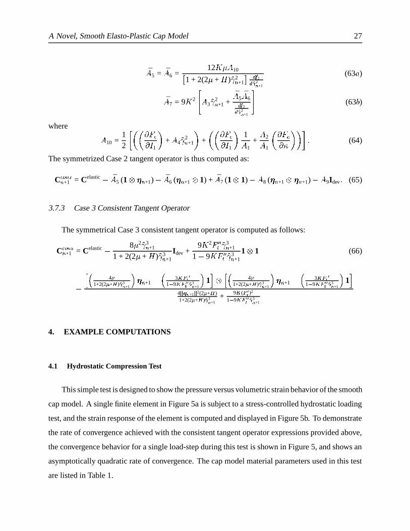
This simple test is designed to show the pressure versus volumetric strain behavior of the smooth
cap model. A single finite element in Figure 5a is subject to a stress-controlled hydrostatic loading
test, and the strain response of the element is computed and displayed in Figure 5b. To demonstrate
the rate of convergence achieved with the consistent tangent operator expressions provided above,
the convergence behavior for a single load-step during this test is shown in Figure 5, and shows an
asymptotically quadratic rate of convergence. The cap model material parameters used in this test
are listed in Table 1.
A Novel, Smooth Elasto-Plastic Cap Model 28
x
y
z
fixed free tomove x
free tomove x,y 1m
1m
1m
P
PP
P
P
a) Mesh and loading conditions.
b) Computed pressure vs. volume strain response of model.
c) Convergence behavior of model.
Pre
ssur
e (M
Pa)
0
2
4
6
8
10
volumetric strain0 0.005 0.01 0.015
consistent tangentcontinuum tangent
104
102
100
10−2
10−4
10−6
resi
dual
nor
m
0 1 2 3 4 5 6iteration number
Figure 5: 5a) Single element mesh for hydrostatic loading test; 5b) pressure versus volumet-ric strain response of the material model; and 5c) finite element force balance convergencecharacteristics of the model during a representative load step, for both the consistent tangentoperator and the continuum tangent operator.
Material Parameter Value
� 170.0 MPa�
210.0 MPa
� � -1.0 KPa� 3.86 KPa� 0.21" 1.2E-6 Pa & 1 0.01
Table 1. Material parameters used in hydrostatic compression test.
A Novel, Smooth Elasto-Plastic Cap Model 29
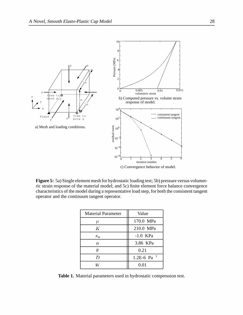
4.2 A Four Element Limit Analysis Computation
While the preceding model demonstrated the performance of the model under purely hydrostatic
loading, this simple four-element test is designed to show the model’s performance under combined
deviatoric and compressive loading. In this test computation, the loading shown on the four-element
mesh (Figure 6a) is increased until the limit state of the model is found using methods outlined
in [20]. The computed load-displacement response of the model is shown in Figure 6b, and the
material model parameters utilized are listed below in Table 2. In this test, which involved plastic
loading at the crown of the cap at the limit state, very good convergence behavior was achieved.
1m
1m
Load
6a) Four element mesh and loading conditions.
6b) Computed load−deformation response.
0 20 40 60 80 100 120 140 160 180
Dis
plac
emen
t (m
*10−
4 )0
−1
−2
−3
−4
−5
−6
−7
Figure 6: 6a) Simple plane-strain four-element mesh with applied loading and restraints;and 6b) the computed load-deformation response provided by the smooth cap model.
Parameter Value Parameter Value
� 208.3 MPa � 0.2003�
500.0 MPa " 3.2E-7 Pa & 1
� � -100.0 KPa 0.15� 12.3 KPa
Table 2. Material parameters used in four element limit analysis test.

A Novel, Smooth Elasto-Plastic Cap Model 30
4.3 Bearing Capacity Computations
In this relatively simple test problem, the bearing capacity of a shallow strip footing foundation
of width�
= 2 � 24 � resting on a sandy soil is computed using the proposed cap model, and the
solutions are compared with analytical results. The bearing capacity computations were performed
using symmetry conditions, and the mesh utilized 600 bilinear continuum elements (Figure 7a).
The problem was solved twice, once for a loose sandy soil ( � 0 = � 10��� � ) and again for a
well-compacted sandy soil ( � 0 = � 1 �� � ). Other than the difference in initial values of � , the
remaining material model parameters used for the loose and dense soils are identical as shown in
Table 3. Before the rigid foundation loading was applied to the soil using displacement control,
the soil deposits were first allowed to consolidate under their own self-weight. Once the soils were
properly stressed in this manner, the loose soil was normally consolidated due to the chosen value
of � 0, while the dense soil would be considered over-consolidated, also due to the chosen value
of � 0. The computed foundation load versus displacement responses for these two soil conditions
are shown in Figure 7b. For the dense sandy soil, a bearing capacity of 0 � 268 ��� was computed,
which compares quite nicely with a bearing capacity of 0 � 260 ��� that would be computed using
Terzaghi’s theory with the assumption of a general shear failure. For the case of the loose sandy
soil, the computed bearing capacity is 0 � 142 ��� which should be compared with the value of
0 � 102 ��� which would be computed using Terzaghi’s model with the assumption of a local shear
failure.
Parameter Value (Loose Sand) Value (Dense Sand)� 2000 kg/m3 2000 kg/m3
� 40.0 MPa 40.0 MPa�
100.0 MPa 100.0 MPa
� � -10.0 KPa -10.0 MPa� 3.86 KPa 3.86 KPa� 0.15 0.15" 3.2E-8 Pa & 1 3.2E-8 Pa & 1 0.1 0.1
Table 3. Sand-like material parameters used in Bearing Capacity Tests. Corresponding to � = 0 � 15,
the Mohr-Coulomb friction angle for the sand would be � = 18 � 89 � .

A Novel, Smooth Elasto-Plastic Cap Model 31
30m
20m
0.5B=1.12m
7a) Mesh used in bearing capacity computations
7b) Computed load-displacement responses for loose sand (dashed) and compacted sand (solid).
κ0 = -10 MPa
κ0 = -10 KPa
Load (MN)
0 0.5 1.0 1.5 2.0 2.5 3.0
Dis
plac
emen
t (m
* 1
0-3)
0
-1
-2
-3
-4
-5
-6
-7
-8
-9
-10
Figure 7: 7a) Mesh of bilinear continuum plane-strain finite elements used in strip footingbearing capacity computations; and 7b) the computed load-displacement response for arigid footing on a loose soil (dashed curve), and on a compacted soil (solid curve).
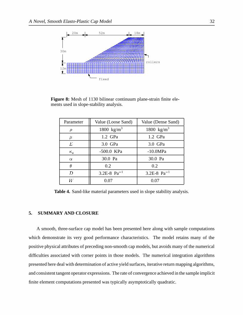
4.4 Slope Stability Analysis Computations
In these computations, an earthen slope model comprised of a sandy soil is analyzed for stability
using the methods proposed in [20], which involve increasing the gravitational loading on the slope
model until a failure mechanism develops, and the slope model can take no further loading. The
mesh used to model the slope is shown in Figure 8 and contains 1130 bilinear continuum plane-
strain finite elements. The finite slope shown has a height of 30m and a repose angle of 29.98 � . For
a loose sandy soil and a dense sandy soil whose parameters are shown in Table 4, the computed
stability factors of safety for this model were 0.95 and 0.98, respectively.
A Novel, Smooth Elasto-Plastic Cap Model 32
fixed
rollers
12m
30m
20m 52m 18m
Figure 8: Mesh of 1130 bilinear continuum plane-strain finite ele-ments used in slope-stability analysis.
Parameter Value (Loose Sand) Value (Dense Sand)� 1800 kg/m3 1800 kg/m3
� 1.2 GPa 1.2 GPa�
3.0 GPa 3.0 GPa
� � -500.0 KPa -10.0MPa� 30.0 Pa 30.0 Pa� 0.2 0.2" 3.2E-8 Pa & 1 3.2E-8 Pa & 1 0.07 0.07
Table 4. Sand-like material parameters used in slope stability analysis.
5. SUMMARY AND CLOSURE
A smooth, three-surface cap model has been presented here along with sample computations
which demonstrate its very good performance characteristics. The model retains many of the
positive physical attributes of preceding non-smooth cap models, but avoids many of the numerical
difficulties associated with corner points in those models. The numerical integration algorithms
presented here deal with determination of active yield surfaces, iterative return mapping algorithms,
and consistent tangent operator expressions. The rate of convergence achieved in the sample implicit
finite element computations presented was typically asymptotically quadratic.

A Novel, Smooth Elasto-Plastic Cap Model 33
Elastoplastic cap models of the type presented here are quite useful in modeling ductile soil
behaviors. To capture softening behaviors in porous media which are also of considerable interest,
cap models such as this one can be straightforwardly coupled with continuum damage mechanics
models.
6. ACKNOWLEDGEMENTS
This research was funded by a University of Iowa Old Gold Fellowship, and by a research
grant from the Whitaker Foundation 96-0636. This support is gratefully acknowledged.
7. BIBLIOGRAPHY
[1] Drucker, D. C. and Prager, W. “ Soil Mechanics and plastic analysis or limit design” Q. Appl. Math., 10(2), 1952,pp. 157-165
[2] Drucker, D. C. “Limit analysis of two- and three-dimensional soil mechanics problems” J. Mech. Phys. Solids,1, 1953, pp. 217-226
[3] Drucker, D. C., Gibson, R. E. and Henkel, D. J. “Soil Mechanics and Work-Hardening Theories of Plasticity”,Transactions, ASCE, Vol. 122, 1957, pp. 1692-1653
[4] Roscoe, K. H., Schofield, A. N. and Worth, C. P. “On the yielding of soils” Geotechnique, 8(1), 1958, pp. 22-53
[5] Roscoe, K. H., Schofield, A. N. and Thurairajah, A. “Yielding of clays in state wetter than critical” Geotechnique,13(3), 1963, pp. 211-240
[6] Schofield, A. N. and Wroth, C. P. “Critical State Soil Mechanics” McGraw-Hill, New York NY, 1968, pp. 310
[7] Burland, J. B. “The yielding and dilation of clay” Correspondence Geotechnique, 15(2), 1965, pp 211-214
[8] DiMaggio, F. L., and Sandler, I. S. “Material models for granular soils”, J. of Engng Mech., ASCE, Vol. 97. No.EM3. June 1971, pp. 935-950
[9] Chen, W. F. “Plasticity in Reinforced Concrete” McGraw-Hill, New York, 1982.
[10] Chen, W.F. and Mizuno, E. “Nonlinear analysis in soil mechanics: theory and implementation,” Elsevier, 1990.
[11] Desai, C. S. and Siriwardane “Constitutive laws for engineering materials” Prentice-Hall, 1984.
[12] Bathe, K.J., Snyder, M.D., Cimento, A.P. and Rolph, W.D. “On some current procedures and difficulties in finiteelement analysis of elasto-plastic response,” Computers & Structures, 12, 1980, pp. 607-624.
[13] Sandler, I. S. and Rubin, D. “ An Algorithm and a modular subroutine for the cap model,” Int’l. J. Numer. Analy.Meth. Geomech., 3, 1979 pp. 173-186
[14] Resende, L. and Martin, J. B. “Formulation of Drucker-Prager cap model” J. Eng. Mech., 111 No. 7., 1985 pp.855-881
[15] Simo, J.C., Kennedy, J.G. and Govindjee, S. “Non-Smooth multisurface viscoplasticity: Loading/unloadingconditions and numerical algorithms” International Journal for Numerical Methods in Engineering, 26 2161-2185(1988).
[16] Ortiz, M. and Simo, J.C. “An analysis of a new class of integration algorithms for elastoplastic constitutiverelations,” International Journal for Numerical Methods in Engineering 23, 1986, 353-366.
[17] Simo, J.C., J-W. Ju, K.S. Pister and R.L. Taylor, Assessment of cap model: consistent return algorithms andrate-dependent extension, Journal of Engineering Mechanics, 114, 1988, 191-218.
[18] G. Hofstetter, J.C. Simo and R.L. Taylor, “A modified cap model: closest point solution algorithms,” Computers& Structures 48-2 203-214 (1993).

A Novel, Smooth Elasto-Plastic Cap Model 34
[19] J. C. Simo and R. L. Taylor, “ Consistent tangent operators for rate-independent elastoplasticity”, ComputerMethods in Applied Mechanics and Engineering, 48 1985, pp. 101-118
[20] C.C. Swan and Y.-K. Seo, “Limit state analysis of earthen slopes using dual continuum/FEM approaches,”International Journal for Numerical and Analytical Methods in Geomechanics, 23 1359-1371 (1999).
[21] Y.-K. Seo and C.C. Swan, “Stability analysis of embankments on saturated soil deposits using elasto-plasticporous medium models,” Journal of Getoechnical and Geoenvironmental Engineering 127-5 436-445 (2001).
[22] O.C. Zienkiewicz, C. Humpheson and R.W. Lewis, “Associated and non-associated viscoplasticity and plasticityin soil mechanics,” Geotechnique 25 671-689 (1975).