a software framework for simulating stationkeeping of a

Modeling, Identification and Control, Vol. 35, No. 4, 2014, pp. 211–248, ISSN 1890–1328

A Software Framework for SimulatingStationkeeping of a Vessel in Discontinuous Ice

Ivan Metrikin

Department of Civil and Transport Engineering, NTNU, N-7491 Trondheim, Norway

Arctic Design and Operations, Statoil ASA, N-7053 Trondheim, Norway

Abstract

This paper describes a numerical package for simulating stationkeeping operations of an offshore vessel infloating sea ice. The software has found broad usage in both academic and industrial projects related todesign and operations of floating structures in the Arctic. Interactions with both intact and broken iceconditions can be simulated by the numerical tool, but the main emphasis is placed on modelling managedice environments relevant for prospective petroleum industry operations in the Arctic. The paper gives athorough description of the numerical tool from both theoretical and software implementation perspectives.Structural meshing, ice field generation, multibody modelling and ice breaking aspects of the model arepresented and discussed. Finally, the main assumptions and limitations of the computational techniquesare elucidated and further work directions are suggested.

Keywords: global ice loads, numerical simulation, physics engine, computational geometry, packingalgorithm

Nomenclature

α Orientation angle of a polygon

αwedge Ice wedge opening angle

β Error reduction parameter

λ Geometrical scaling factor

Ipolygon List of intersection polygons between thevessel and an ice floe polygon

Spolygon List of intersection polygons between thevessel and the top plane of an ice floe

µk Coefficient of kinetic friction

µs Coefficient of static friction

ρ Density of a medium

σc Compressive strength of ice

σf Flexural strength of ice

σmaxwedge Maximal bending stress in a wedge-shaped icebeam resting on an elastic foundation

σyy Bending stress in a semi-infinite ice sheet

θcrack Polar angle of the splitting crack

4t Time step

~λ Vector of Lagrange multipliers of the multibodysystem

~Ω Angular velocity of a body

~τ Torque acting on a body

~bbox Object-aligned bounding box vector

~bpen Position correction vector of the multibody sys-tem

doi:10.4173/mic.2014.4.2 c© 2014 Norwegian Society of Automatic Control

http://dx.doi.org/10.4173/mic.2014.4.2

Modeling, Identification and Control

~dbest Maximal scaling factor for a polygon in the icefield generation algorithm

~dmax Maximal floe size

~dmin Minimal floe size

~dscale Scaling vector in the ice field generation algo-rithm

~F Force vector of the multibody system

~f Force acting on a body

~g Acceleration of gravity

~n Contact normal

~n4 Normal to an intersection point between thevessel and an ice floe

~nbreak First possible crack propagation direction

~npolygon Normal of an intersection polygon betweenthe vessel and an ice floe

~nsplit Splitting crack direction vector

~p Constraint impulse vector

~r Coordinate of a point

~u Velocity vector of the multibody system

~v Linear velocity of a body

A Area of a geometrical shape

b Thickness of an artificial boundary around theice field region

Ca Angular drag coefficient

Cd Form drag coefficient

Cs Skin friction coefficient

dlim Ice floe narrowness threshold

dpen Penetration depth in a contact point

e Coefficient of restitution

F Friction coefficient matrix of the multibody sys-tem

H Kinematic map matrix of the multibody system

hi Ice thickness

I Inertia tensor of a body

I3×3 3-by-3 unit matrix

J Constraint Jacobian matrix of the multibodysystem

jpos Positional noise in the ice field generation algo-rithm

jrot Rotational noise in the ice field generation al-gorithm

kd Constraint damping factor

ks Constraint stiffness factor

L Length of a region

l Length of an object

lavg Average length of a fluid mesh

Lbreakable Ice floe breakability length

M Inertia matrix of the multibody system

m Mass of an object

Nbody Amount of bodies in the simulation

N interscontact Amount of contact points associated with an

intersection polygon between the vessel and anice floe

Ncont Amount of contacts in the multibody system

Nexpand Amount of attempts to expand a polygon inthe ice field generation algorithm

Nfails Amount of attempts to place a polygon in theice field generation algorithm

Njoint Amount of joints in the multibody system

Nsize Amount of the floe size sub-intervals in the icefield generation algorithm

Ntrials Amount of attempts to perturb a polygon inthe ice field generation algorithm

Nver Amount of polygon vertices in the ice field gen-eration algorithm

Nwedges Amount of ice wedges in a circumferentialcrack

plim Limiting impulse of the ice crushing constraint

Q A quaternion

qload Areal density of the distributed load acting ona semi-infinite ice plate

R Rotation matrix of a body

r, p, q Cardan angles

212

Metrikin I., “A Software Framework for Simulating Stationkeeping of a Vessel in Discontinuous Ice”

Rbending Circumferential crack radius

Rload Radius of the loaded area on a semi-infinite iceplate

Sk Splitting radius multiplication coefficient

T Transformation matrix of a body

t Length of a line segment in the polygon gener-ation algorithm

V Volume of a geometrical shape

vproj Linear velocity projection on a surface

W Width of a region

w Width of an object

X,Y, Z Axes of a Cartesian reference frame

x, y, z Coordinates in a Cartesian reference frame

1 Introduction

The majority of prospective hydrocarbon deposits inthe Arctic are located offshore, beyond the 100-m wa-ter depth contour, which is considered to be the upperlimit for bottom-founded structures in areas with pos-sible sea ice intrusions (Hamilton, 2011). Operations insuch areas require robust floating drilling and produc-tion systems, supported by a reliable fleet of ice man-agement, supply, emergency response and interventionvessels. Upcoming oil and gas activities require thesefloating structures to withstand environmental loads,including those from sea ice.

Although it is anticipated that the first upcomingoil and gas operations in deep-water Arctic areas willtake place primarily within the open water season, seaice intrusions may occur under some circumstances. Ifthis happens, it is expected that the ice managementfleet will be able to break down the incoming ice floesinto acceptable sizes, such that the stationkeeping per-formance of the platform would not be compromised.Therefore, the ice cover approaching the operationalsite will be discontinuous, i.e. broken into discrete icefeatures of various shapes and sizes.

The ability of a platform to hold its position duringa sea ice intrusion event is governed by the relationshipbetween the global environmental load from broken iceand the stationkeeping system capacity. The ice loaddepends on the structure-ice interaction process whichinvolves complex contact mechanics: ice material fail-ure, rigid-body motion of the broken ice pieces, ice-iceand ice-structure friction and fluid effects. Moreover,the boundary conditions of the managed ice domain

have an influence on the load-response relationship ofthe dynamical system, leading to highly nonlinear andcomplex behavior.

Full-scale data obtained during the Kulluk platformoperations (Wright, 1999) indicates that stationkeep-ing in managed ice is possible, and the mooring systemloads measured during Kulluk operations can be usedto perform analytical estimates of the global ice loadsfor design purposes (Palmer and Croasdale, 2013).However, such estimates have not been validated byfull-scale data for the case of ship-shaped structures,which are currently considered attractive for Arcticdeep-water exploration. Therefore, ice tank experi-ments are usually performed on new designs to estab-lish the global loads and operational envelopes of float-ing offshore structures in various sea ice conditions.

Although model testing is currently considered tobe the state-of-the-art method for estimating globalice loads, it has some limitations. Scaling uncertain-ties and boundary effects are the most challengingones when testing floaters in broken ice, especiallyvertically-sided ship-shaped structures. For example,the author of this paper has experienced a 7-meter-longvessel moored at 30 oblique angle relative to the icedrift to induce a boundary interaction in a 10-meter-wide ice tank after just first 3 meters of a model exper-iment. Therefore, it seems attractive to develop a nu-merical model for simulating such interactions, validateit against model-scale data, and then use the validatedmodel to expand the testing environment (for exampleto increase the width of the ice basin). Moreover, suchmodel could be used for pre-simulating the model testsand optimizing the amount of physical experiments inadvance of the actual testing campaign.

Such numerical model has been developed withinthe framework of the DYPIC (Kerkeni et al., 2014)and Arctic Dynamic Positioning (DP) (Skjetne, 2014)projects. The initial goal of the model was to run morescenarios than during the laboratory testing campaignof the DYPIC project at the large ice tank of the Ham-burg Ship Model Basin (HSVA). Therefore, the modelwas given a preliminary name ”Numerical Ice Tank”,as it was tailored to replicate model-scale experimentsat HSVA. However, the latest version of the model sup-ports also full-scale simulations, as reported in Scibiliaet al. (2014).

To the best of the author’s knowledge, the first nu-merical ice tank concept was proposed by Valanto andPuntigliano (1997) to simulate the icebreaking resis-tance of a ship in level ice. That paper suggested anapproach which separated the icebreaking process atthe design waterline of a vessel from the motions of thebroken ice floes under the hull. Later, Derradji-Aouat(2010) described a fully coupled numerical ice tank en-

213

http://dypic.eu/

http://www.marin.ntnu.no/arctic-dp/


vironment based on Explicit Finite Element Methodimplemented within commercial packages ANSYS andLS-DYNA. This technique was used by Wang andDerradji-Aouat (2010) and Wang and Derradji-Aouat(2011) to simulate model-scale and full-scale interac-tions of structures with broken ice. However, althoughthe approach proposed by Derradji-Aouat (2010) isgeneric, the ice pieces were considered unbreakable inthose examples. Finally, Lee et al. (2013) proposed anumerical ice tank based on the multi-material arbi-trary Lagrangian formulation and the fluid-structureinteraction analysis technique of the LS-DYNA code.Pre-sawn level ice tests of 2 different hull shapes weresuccessfully simulated in that paper.

The main differences of the current model from theother numerical ice tanks is the assumption of low in-teraction velocities between the vessel and the ice (i.e.below 2 m/s in full-scale), and the focus on modellingbroken ice conditions. The former assumption leads toa simplified treatment of hydrodynamic interactions,because the ice breaking phenomena become more aproblem of solid mechanics rather than hydrodynam-ics. The latter leads to adoption of the physics en-gine software for collision detection, contact force com-putation and time stepping of the numerical model.From the theoretical perspective, the physics engineapproach is equivalent to the nonsmooth discrete ele-ment method (Metrikin and Løset, 2013). The maindifference of the nonsmooth discrete element methodfrom the conventional penalty-based discrete elementmethod is that the stiffness and damping parametersdo not need to be introduced into the contact problemformulations. Therefore, larger time steps can be usedand a higher computational efficiency can be achievedin the numerical tool. A detailed comparison of thetwo different discrete element methods can be foundin e.g. Servin et al. (2014). Discrete treatment of theice features allows the model to calculate the ice loadsdue to breaking, rotation, submergence and sliding ex-plicitly, i.e. the motions of the broken ice floes underand around the hull are fully modelled. This is an-other major difference of the current model from thecommonly used ice material transport formulations ofLindqvist and Croasdale (Su, 2011; Bonnemaire et al.,2011). The simulated ice failure modes in the currentmodel include crushing, flexural bending and splitting.Therefore, although the model is tailored to simulat-ing broken ice conditions, it is also capable of modellingfixed and floating offshore structures interacting withintact ice.

The software package has been broadly used by theindustry and academia to investigate design and oper-ations of floating Arctic offshore structures. Metrikinet al. (2013b) used the first version of the model for

simulating dynamic positioning of an Arctic drillshipin managed ice and compared the modelling resultswith model testing data. Later, Kerkeni et al. (2013a)used the model to compare the DP control laws in openwater and ice, and to establish DP capability plots of avessel in managed ice (Kerkeni et al., 2013b). Metrikinand Løset (2013) simulated an oblique towing test ofan Arctic drillship in managed ice and compared sim-ulation results to experimental data. Later, Metrikinet al. (2013a) performed the first simulation of DP inlevel ice and Kerkeni and Metrikin (2013) proposed anautomatic heading controller for managed ice condi-tions, together with its verification by numerical sim-ulations. Finally, Scibilia et al. (2014) simulated theicebreaker Oden in full-scale broken ice conditions off-shore North-East Greenland, Østhus (2014) developedan adaptive control methodology for a vessel in man-aged ice using hybrid position and force control, andKjerstad and Skjetne (2014) performed modeling andcontrol of a DP vessel in curvilinearly drifting managedice. Full development timeline of the model is outlinedin Kerkeni et al. (2014).

Currently, the binary version of the software hasbeen released to commercial partners of the DYPICand Arctic DP projects, while the source code and in-tellectual property rights of the model are owned bythe Norwegian University of Science and Technology.

This paper describes the numerical tool from boththeoretical and software implementation perspectives.First, Section 2 gives a high-level overview of the sim-ulation model and its main components. Next, Section3 describes the preparation steps the user has to takefor executing a simulation run. Then, Section 4 out-lines the initialization sequence of the numerical model,including structural creation and ice field generation.Afterwards, Section 5 specifies the theoretical aspectsof the actual simulation process, including the multi-body dynamics model, the fluid force model and theice breaking model. Then, Section 6 presents the out-put functionalities of the simulator. Finally, Section7 discusses the main assumptions and limitations ofthe computational approach, and Section 8 summarizesand concludes the paper.

2 Simulator Overview

On the highest level the simulator is structured asshown in Figure 1. The user sets up a simulation in thesoftware by creating an input file for the pre-processor.The structure and contents of this file are discussed inSection 3.1. Then, the user should perform the meshingof the simulated vessel according to a special processoutlined in Section 3.2. Finally, the actual simulationprogram starts by initializing the physical scene (Sec-

214


tion 4) and entering the simulation loop (Section 5).S

imul

atio

n lo

op

Input File(XML)

Initialization

Physical Engine

Visualization CSV

Post-processing

Simulation setup

StructuralMeshing

Figure 1: Simulation workflow of the numerical model.

The simulation loop is centered around the physi-cal engine middleware. This software development kit(SDK) is used to perform collision detection, contactmanifold creation, rigid body and joint dynamics com-putation, contact force evaluation and time integrationof the equations of motion. Metrikin et al. (2012b) de-scribed a framework for modelling a floating structurein broken ice using a physical engine, and Metrikinet al. (2012a) performed a comparative study of dif-ferent physical engines for simulating ice-structure in-teractions. Later it was realized that physical enginesare being constantly developed and improved, and onesolution might become outdated in a very short time.Therefore, it was decided to base the software packageon a generic interface that would support any physicalengine, so that the user could easily switch betweenthe different engines and integrate new ones when nec-essary. Such interface has been implemented usingthe Physics Abstraction Layer (PAL) library (Boeing,2009), which provides a unified interface to many differ-ent physical engines. The PAL library is implementedas a C++ abstract pluggable factory which maintainsa common registry of physical objects that can be sim-ulated by all underlying physical engines. When a cer-tain engine is selected by the user, the registry is popu-lated with objects and methods for that specific engineduring run-time of the application. Further description

of the physical engine itself, including the theoreticalbackground, is given in Section 5.

Optional visualization of the simulation scene canbe performed by the software in real-time using the Ir-rlicht library (Gebhardt et al., 2012) (Section 6.2). Fur-thermore, the simulator can produce numerical outputdata in comma-separated format (CSV) for subsequentanalysis and post-processing by the user (Section 6.1).

The full numerical model is packaged into a 32-bitdouble-precision Microsoft Windows application. Ithas been developed in C++ programming languageusing Microsoft Visual Studio 2010 development en-vironment, and the Microsoft Visual C++ runtimeis needed to run the software on the user’s machine.The C++ Standard Library has been used for memorymanagement (e.g. smart pointers), exception handling,input/output streaming, textual string processing, nu-merical functions (e.g. square root), container manage-ment (e.g. vectors, maps, sets and their algorithms)and templates. Version 3 of the Boost.Filesystem li-brary (Dawes, 2012) has been used to manipulate files,directories and system paths for the majority of in-put/output tasks in the software. Finally, the buildsystem of the application has been implemented usingWindows batch scripting, and the source code lifecyclehas been managed using the Subversion (SVN) tech-nology.

3 Simulation Setup

This section describes the pre-processing steps requiredfor the user to set up a simulation in the software pack-age.

3.1 Input File Preparation

The input file for the software tool has an ExtensibleMarkup Language (XML) format and contains all es-sential information for initializing the numerical model.Loading and parsing of the input file is implementedusing version 1.2 of the PugiXML library (Kapoulkine,2014). There are 3 sections in the input file: overallsimulation settings, scene settings and output settings.The contents of these sections are described in the fol-lowing paragraphs.

Firstly, the overall simulation settings contain thename of the physical engine to use in the simulationloop. The user can select between AgX Dynamics (Al-goryx Simulation AB, 2014), Bullet Physics (Coumans,2012), Open Dynamics Engine (Smith, 2014), NVIDIAPhysX (Nvidia Corporation, 2014) and Vortex Dynam-ics (CM Labs Simulations Inc., 2014) libraries. How-ever, the ice breaking functionality is currently sup-ported only in the Bullet-based implementation of the

215


numerical tool. Therefore, if the user selects any engineexcept Bullet, the ice floes will be treated as unbreak-able (see Section 5 for more details on ice breaking).

Furthermore, the overall simulation settings sectionof the input file contains the amount of CPU threadsto run (the application supports multithreading), thesize of the time step, the total amount of time steps tosimulate and the real-time visualization system settings(i.e. the target, heading, elevation and distance to thecamera in the global spherical coordinate system).

The scene settings of the input XML file contain thefollowing parameters:

• Properties of the simulated vessel: geome-try, mass, inertia tensor and initial posi-tion/orientation;

• Physical size of the virtual ice tank: length, widthand depth;

• Acceleration of gravity defined as a 3D vector inthe global reference frame;

• Ice properties: density, thickness, compressive andflexural strength values and Youngs modulus;

• Fluid properties: density, drag coefficients andtype of the angular drag model (see Section 5.3);

• Mechanical contact properties for the various pairsof contact surfaces: ice-ice, ice-structure and ice-boundary (e.g. static and dynamic friction coeffi-cients, possible restitution and stiffness/dampingin constraints - see Section 5);

• The ice field is defined inside a specified rectan-gular region which is characterized by the type ofthe ice feature (intact or broken), target ice con-centration in %, floe size distribution and the seedof random number generator for the packing algo-rithm (Section 4.3);

• Simulation type: free running, oblique towing ordynamic positioning (DP). The DP system inter-face is implemented as a static library component(a set of .lib files) which can be linked by the userinto a custom-made control system project. Boththe simulation and visualization processes can becontrolled by the user through this interface. Atthe start of every time step of a DP simulation thesimulator receives actuation inputs in surge, swayand yaw DOFs and sums them additively with anyother external forces acting on the vessel to obtainthe total load (see Metrikin et al. (2013b), Kjer-stad and Skjetne (2014) and Section 5). A moor-ing system or any other external forces acting onthe vessel can also be implemented through thisDP interface.

Finally, in the output settings section of the inputXML file the user specifies the system path to the out-put CSV file; the components of the position, orienta-tion, force and torque vectors of the vessel to recordat every time step (computed in the global referenceframe, as described in Section 6.1); and the amount ofnumerical digits after the decimal point for all outputvalues (the software can output numerical values up tomachine precision).

3.2 Structural Meshing

The geometry of the vessel is also specified in the scenesettings section of the input XML file. In the simula-tion it is represented by 2 different triangulated surfacemeshes: a fluid mesh (Figure 2) and a collision mesh(Figure 3). If the user would like to run model-scalesimulations, it is possible to specify a scaling factorfor the meshes in the input XML file. The simulatorwill then grow or shrink both meshes to the desiredgeometrical scaling factor λ.

Figure 2: Fluid mesh of a conceptual Arctic drillship(courtesy Statoil).

Figure 3: Collision mesh of a conceptual Arctic drill-ship (courtesy Statoil). Different colors rep-resent different convex decomposition pieces.

The fluid mesh is used for calculating the inertiatensor of the vessel and the fluid forces acting on it(see Section 5.3), while the collision mesh is used toconstruct a geometrical representation of the vessel fordetecting contacts with the ice floes in the physical en-gine. The simulator does not support concave collisionmeshes, so if there are any concavities in the originalcollision mesh, it must be decomposed into convex ele-ments (otherwise the collision detection system of thephysical engines will either fail or work very slowly).

216


Some automatic convex decomposition tools are avail-able for this task, e.g. the Hierarchical ApproximateConvex Decomposition tool (Mamou, 2013). However,experience shows that although such tools can pro-vide a reasonable initial convex decomposition, the fi-nal refinement has to be performed manually using a3D computer graphics software package (such as 3dsMax (Autodesk, 2014) or Blender (Blender Founda-tion, 2014)). Throughout the manual refinement pro-cess it is very important to constantly ensure that whenthe convex pieces are added together they will repre-sent the original mesh as closely as possible. Commonpractice is to use the original concave fluid mesh as areference for the convex-decomposed collision mesh.

The geometrical file format used by the simulator isWavefront OBJ, and files constituting both the fluidand collision meshes should be supplied in this format.The physical engines need only the vertex coordinatesof the convex collision meshes for their construction,while fluid meshes require the face indices in additionto vertex coordinates. Currently, due to limitationsof the OBJ file loader in the application, all meshescan have only triangular faces (the file loader is im-plemented using an open source library developed byLindenhof (2012)). Furthermore, before starting a sim-ulation it is recommended to pre-process the meshesso that they contain as few faces as possible, in orderto reduce the computational burden on the simulator.Moreover, the user must ensure that the meshes areclosed (i.e. every edge has exactly 2 adjacent triangu-lar faces) and do not contain any holes, otherwise thecollision detection system will have artifacts. Finally,degenerate features, such as too narrow triangles orduplicate surfaces, must be removed from the meshesin order to avoid degenerate collision configurations.It is worth mentioning that the author’s experience inusing the simulator indicates that mesh preparation iscurrently the most time-consuming part of the wholesimulation setup process.

4 Initialization of the SimulationScene

The simulation scene in the numerical model contains5 physical components: the fluid domain, the vessel,the ice field, the boundaries and, optionally, the tow-ing carriage (Figure 4). The global coordinate systemXg, Yg, Zg is assumed inertial, while local coordinatesystems of the structure Xs, Ys, Zs and the ice floesXi, Yi, Zi are moving attached to their respective ob-jects.

Initialization of the scene is performed stepwise,starting from creation of the boundaries which demar-

cate a rectangular region in the Xg, Yg plane whereall simulated objects will be confined (Figure 5). Thelength L and width W of this region are specified bythe user in the input file. The boundaries are repre-sented by static rectangular cuboids in the simulation,meaning that they constitute immovable rigid objectsin the physical engine. The height of the cuboids de-fines the depth of the virtual ice tank, as specified bythe user in the input file.

Yg

Xg W

L

Figure 5: Boundaries of the simulation domain.

Next, the fluid domain is created. It is representedby a static half-space demarcated by the Xg, Ygplane, i.e. the water level is always at Zg = 0. Thewhole underwater domain is assigned a uniform con-stant density, as specified by the user in the input file.All objects in contact with the fluid are affected bybuoyancy and drag forces which are computed accord-ing to a method described in Section 5.3.

The following sub-sections describe the creation ofthe vessel (Section 4.1), the towing carriage (Sec-tion 4.2) and the ice field (Section 4.3). However, be-fore these objects are constructed, the simulator ini-tializes the contact property table in the selected phys-ical engine using the PAL interface. For every coupleof contacting surfaces (ice-ice, ice-structure and ice-boundary), the following values are populated from theinput file: static friction coefficient µs, kinetic frictioncoefficient µk, restitution coefficient e, constraint stiff-ness factor ks and constraint damping factor kd. When2 objects experience a pairwise collision this table isused to define their interaction mechanics according tothe contact dynamics method (Section 5).

4.1 Vessel Creation

Creation of the vessel in the numerical model is a step-wise process. First of all, the fluid and collision meshesare loaded from their respective Wavefront OBJ files,and geometrical scaling of the vertices is performed:~r newi = λ~r oldi , where ~r oldi is the original 3D coordinateof vertex i in the local coordinate system of the mesh,

217


Xg Yg

Zg

Xs Ys

Zs

Xi

Yi

Zi

Figure 4: Simulation scene of the numerical model.

λ is the geometrical scaling factor from the input fileand ~r newi is the scaled coordinate of the vertex. Af-ter the scaling operation, each convex decompositionpiece is converted into a point cloud with unique ver-tices, because the convex mesh loader of the applicationremoves triangulation and discards duplicate verticesfrom the collision meshes of the vessel.

Secondly, the body of the vessel is created in thephysical engine through the PAL interface. Its collisiongeometry becomes a compound shape consisting of theprovided convex pieces, and the fluid mesh is used tocalculate the inertial properties of the body accordingto the following algorithm:

1. The signed volume of each tetrahedron in the fluidmesh is computed as follows:

V i4 =1

6~r i1 · [(~r i2 − ~r i1)× (~r i3 − ~r i1)]

where ~r i1,2,3 are 3D vertex coordinates of trianglei in the local coordinate system of the mesh, andthe apex of the tetrahedron is assumed to coincidewith the origin of this coordinate system. The ·sign represents vector dot product, and the × signrepresents vector cross product.

2. Center of mass of every tetrahedron is calculatedin the local coordinate system of the mesh as fol-lows:

~r4i

CoM =1

4(~r i1 + ~r i2 + ~r i3)

3. The total volume of the mesh is calculated by ac-cumulating the signed volumes of every tetrahe-dron:

V =∑i

V i4

4. The center of mass of the whole mesh is calcu-lated in the local coordinate system of the meshas follows:

~rCoM =1

V

∑i

~r4i

CoMVi4

5. An auxiliary 3D vector ~d is computed for everytriangle in the mesh:

~d i = (~r i1)2 +(~r i2)2 +(~r i3)2 +~r i1 ~r i2 +~r i1 ~r i3 +~r i2 ~r i3

where the sign represents the Hadamard vectorproduct.

6. Components of the inertia tensor of each unit-masstetrahedron are computed in the local coordinate

218


system of the mesh using the method of Tonon(2005):

I4i

11 =diy + diz

10

I4i

22 =dix + diz

10

I4i

33 =dix + diy

10

I4i

12 = I4i

21 = − 1

20·

·(2ri1,xri1,y + ri2,xri1,y + ri3,xr

i1,y+

+ri1,xri2,y + 2ri2,xr

i2,y + ri3,xr

i2,y+

+ri1,xri3,y + ri2,xr

i3,y + 2ri3,xr

i3,y)

I4i

13 = I4i

31 = − 1

20·

·(2ri1,xri1,z + ri2,xri1,z + ri3,xr

i1,z+

+ri1,xri2,z + 2ri2,xr

i2,z + ri3,xr

i2,z+

+ri1,xri3,z + ri2,xr

i3,z + 2ri3,xr

i3,z)

I4i

23 = I4i

32 = − 1

20·

·(2ri1,yri1,z + ri2,yri1,z + ri3,yr

i1,z+

+ri1,yri2,z + 2ri2,yr

i2,z + ri3,yr

i2,z+

+ri1,yri3,z + ri2,yr

i3,z + 2ri3,yr

i3,z)

7. Inertia tensor of the unit-mass mesh about the ori-gin is computed as follows:

Io =∑i

I4iV i4

8. Inertia tensor about the center of mass is calcu-lated using the parallel axis theorem:

ICoM = ρ[Io − V ·· (~r 2

CoMI3×3 − ~rCoM ⊗ ~rCoM )]

where

ρ = m/V is the density of the vessel (the soft-ware tool assumes uniform distribution of massm), I3×3 is a 3-by-3 unit matrix and the ⊗ signrepresents the outer vector product.

9. The principal axes of the body are found using theJacobi eigenvalue algorithm ICoM = RIdiagCoMR

T ,where

R =

R11 R12 R13

R21 R22 R23

R31 R32 R33

is the rotation matrix to the principal axes of thebody (composed from the eigenvectors of ICoM ),

and IdiagCoM is the diagonalized inertia tensor (com-posed from the eigenvalues of ICoM ). The Jacobiiteration stops when all off-diagonal elements areless than the threshold value of 10−12 multipliedby the sum of the absolute values on the diagonal,or when the limit of 20 iterations is reached. Itis possible to use this algorithm for inertia tensordiagonalization because ICoM is a real symmetricmatrix.

In the subsequent simulation, the origin of the localcoordinate system of the vessel Xs, Ys, Zs is alwayskept at the center of mass ~rCoM and its orientation iskept equal to the principal axes orientation, such thatthe inertia tensor is constant and diagonal (equal to

IdiagCoM ). The software ensures that both the fluid andthe collision meshes are always synchronized with thiscoordinate system.

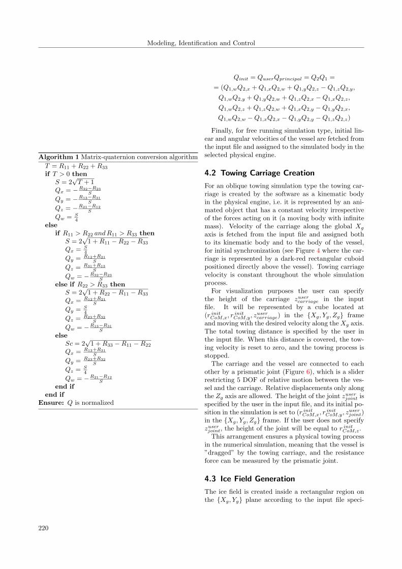
The simulator uses unit quaternions to representrotations during the dynamical simulation process.Therefore, the rotation matrix to the principal axesR is converted to a unit quaternion Qprincipal =Qx, Qy, Qz, Qw using Algorithm 1. The algorithmensures a non-degenerative production of a unit quater-nion to represent rotation matrix R.

Initial position and orientation of the vessel in thesimulator are given by the user in the input file as the3D coordinate of the center of mass ~r initCoM in the globalframe Xg, Yg, Zg and 3 Cardan angles r, p, q in ra-dians. The software converts these angles into a unitquaternion as follows:

Quser = (sinr

2cos

p

2cos

y

2− cos

r

2sin

p

2sin

y

2,

cosr

2sin

p

2cos

y

2+ sin

r

2cos

p

2sin

y

2,

cosr

2cos

p

2sin

y

2− sin

r

2sin

p

2cos

y

2,

cosr

2cos

p

2cos

y

2+ sin

r

2sin

p

2sin

y

2)

Then, initial quaternion of the simulated vessel iscomputed by applying the user-defined rotation to theprincipal axes of the body using quaternion multipli-cation operation:

219


Algorithm 1 Matrix-quaternion conversion algorithm

T = R11 +R22 +R33

if T > 0 thenS = 2

√T + 1

Qx = −R32−R23

S

Qy = −R13−R31

S

Qz = −R21−R12

S

Qw = S4

elseif R11 > R22 andR11 > R33 then

S = 2√

1 +R11 −R22 −R33

Qx = S4

Qy = R12+R21

S

Qz = R31+R13

S

Qw = −R32−R23

Selse if R22 > R33 then

S = 2√

1 +R22 −R11 −R33

Qx = R12+R21

S

Qy = S4

Qz = R23+R32

S

Qw = −R13−R31

Selse

Sc = 2√

1 +R33 −R11 −R22

Qx = R13+R31

S

Qy = R23+R32

S

Qz = S4

Qw = −R21−R12

Send if

end ifEnsure: Q is normalized

Qinit = QuserQprincipal = Q2Q1 =

= (Q1,wQ2,x +Q1,xQ2,w +Q1,yQ2,z −Q1,zQ2,y,

Q1,wQ2,y +Q1,yQ2,w +Q1,zQ2,x −Q1,xQ2,z,

Q1,wQ2,z +Q1,zQ2,w +Q1,xQ2,y −Q1,yQ2,x,

Q1,wQ2,w −Q1,xQ2,x −Q1,yQ2,y −Q1,zQ2,z)

Finally, for free running simulation type, initial lin-ear and angular velocities of the vessel are fetched fromthe input file and assigned to the simulated body in theselected physical engine.

4.2 Towing Carriage Creation

For an oblique towing simulation type the towing car-riage is created by the software as a kinematic bodyin the physical engine, i.e. it is represented by an ani-mated object that has a constant velocity irrespectiveof the forces acting on it (a moving body with infinitemass). Velocity of the carriage along the global Xg

axis is fetched from the input file and assigned bothto its kinematic body and to the body of the vessel,for initial synchronization (see Figure 4 where the car-riage is represented by a dark-red rectangular cuboidpositioned directly above the vessel). Towing carriagevelocity is constant throughout the whole simulationprocess.

For visualization purposes the user can specifythe height of the carriage zusercarriage in the inputfile. It will be represented by a cube located at(r initCoM,x, r

initCoM,y, z

usercarriage) in the Xg, Yg, Zg frame

and moving with the desired velocity along the Xg axis.The total towing distance is specified by the user inthe input file. When this distance is covered, the tow-ing velocity is reset to zero, and the towing process isstopped.

The carriage and the vessel are connected to eachother by a prismatic joint (Figure 6), which is a sliderrestricting 5 DOF of relative motion between the ves-sel and the carriage. Relative displacements only alongthe Zg axis are allowed. The height of the joint zuserjoint isspecified by the user in the input file, and its initial po-sition in the simulation is set to (r initCoM,x, r

initCoM,y, z

userjoint)

in the Xg, Yg, Zg frame. If the user does not specifyzuserjoint, the height of the joint will be equal to r initCoM,z.

This arrangement ensures a physical towing processin the numerical simulation, meaning that the vessel is”dragged” by the towing carriage, and the resistanceforce can be measured by the prismatic joint.

4.3 Ice Field Generation

The ice field is created inside a rectangular region onthe Xg, Yg plane according to the input file speci-

220


Figure 6: A horizontally aligned prismatic joint(Coumans, 2014).

fication. Before generating the ice field the softwarechecks that the requested rectangular region of the icefield is fully contained inside the ice tank boundaries(Figure 11), so that no ice floes fall outside the ac-tually simulated domain. Within the ice field rectan-gle the numerical tool can generate a level ice sheet(Section 4.3.1) or 3 different types of broken ice fields:randomly-distributed (Section 4.3.2), grid-distributedor size-distributed. The latter 2 are not discussed inthis paper.

After the 2D ice field generation step is completedeach ice floe polygon is positioned in the Xg, Ygplane. Then, all ice floes are created as dynamic bodiesin the selected physical engine, i.e. their collision andfluid meshes are generated. Collision meshes are ob-tained by extruding the 2D polygonal shapes of the icefloes along the Zg axis to obtain a uniform thicknesshi according to the input file specification. The resultof the extrusion operation is a set of polyhedral rigidbodies with their side faces parallel to the Zg axis (Fig-ure 7). These polyhedra are used as collision meshes ofthe ice floes during the following dynamical simulationprocess.

Top face

Side faces

Figure 7: Ice floes in the virtual ice tank.

Fluid meshes of the ice floes are created differentlyfor rectangular and polygonal geometries. Rectangularice floe meshes are generated by manually triangulat-ing their faces (Figure 8, a-d), while polygonal ice floesare first triangulated in-plane using a constrained De-launay triangulation library Poly2Tri (Green, 2013):Figure 9, a-b. Then, the triangulated polygon is du-plicated to create an extruded 3D prism of thicknesshi, which will constitute the top and bottom faces ofthe fluid mesh (Figure 9, c). Finally, the side faces ofthe polyhedron are triangulated to complete the mesh(Figure 9, d).

Figure 8: Rectangular cuboid triangulation.

Inertial properties of the rectangular ice floes arecomputed using analytical formulae. The mass is cal-culated as follows: mi = LiWihiρi, where ρi is theice density. Inertia tensor about the principal axes iscomputed as follows:

Ibox = mi/12

L2i + h2i 0 0

0 W 2i + h2i 0

0 0 L2i +W 2

i

The principal axes themselves are parallel to the sidesof the rectangular cuboid (Figure 10). The origin of theprincipal axes is located at the center of mass, whichin this case coincides with the geometrical center (reddot in Figure 10).

Inertial properties of polyhedral ice floes are calcu-lated using their fluid meshes and the same techniquesas for the vessel (Section 4.1, steps 1-9). The onlydifference is that in step 8 of the algorithm the icedensity is used instead of the structural density (it is

221


Figure 9: Polyhedron triangulation.

assumed that the ice floes have uniform density andtheir mass can be computed as mi = A2Dhiρi, whereA2D is the area of the ice floe polygon). Otherwise,the exact same source code is used for the ice floes andthe vessel. Furthermore, in the same manner as forthe vessel, the simulator ensures that the origin of thelocal coordinate system of the ice floes Xi, Yi, Zi isalways kept at the center of mass, and its orientation isalways kept equal to the principal axes, such that theinertia tensor in the local frame remains constant anddiagonal throughout the whole simulation process.

hi

Li Wi

XiYi

Zi

Figure 10: Dimensions of a rectangular cuboid.

The software initializes the vertical positions of theice floes such that their draft is equal to hi

ρiρw

, where ρwis the water density. Therefore, at the start of the sim-ulation process all ice floes are created in equilibriumwith the fluid. Additionally, the ice field generation al-gorithm ensures that the ice floes do not intersect each

other and do not physically interact with each other atthe start of the simulation process (Section 4.3.2).

To create the ice floes in the physical engine throughthe PAL interface, their initial positions and orienta-tions have to be converted into PAL 4 × 4 matrices.To achieve this, first, the orientation quaternion ofan ice floe is generated from its axis-angle represen-tation: Q = (kx sin α

2 , ky sin α2 , kz sin α

2 , cos α2 ). Sincekx = ky = 0, kz = 1, this expression simplifies toQ = (0, 0, sin α

2 , cos α2 ), where α is the rotation angle ofthe ice floe around the Zg axis. Then, a 3× 3 rotationmatrix is generated from the quaternion:

R =

1− 2

Q2y+Q

2z

‖Q‖2 2QxQy+QwQz

‖Q‖2 2QxQz−QwQy

‖Q‖2

2QxQy−QwQz

‖Q‖2 1− 2Q2

x+Q2z

‖Q‖2 2QyQz+QwQx

‖Q‖2

2QxQz+QwQy

‖Q‖2 2QyQz−QwQx

‖Q‖2 1− 2Q2

x+Q2y

‖Q‖2

where ‖Q‖2 = Q2

x +Q2y +Q2

z +Q2w. Finally, the 4× 4

transformation matrix for the PAL interface is com-puted as follows:

T =

R11 R12 R13 0R21 R22 R23 0R31 R32 R33 0rx ry rz 1

where ~r = (rx, ry, rz)

T is the 3D position vector of theice floe’s center of mass. The resulting matrix T is usedfor initializing every ice floe in the selected physicalengine.

4.3.1 Level Ice Field Generation

The level ice field is generated as a rectangular regionextruded along the Zg axis and uniformly filled withthe ice material of thickness hi. In the physical engineit is represented by a static rectangular cuboid whichis not affected by forces from any other objects in thesimulation domain (same rigid body type as the icetank walls). However, the level ice itself can breakand can produce reaction forces on the vessel and thedynamic ice pieces in contact with it. The ice forcecomputation algorithms are described in Section 5.

4.3.2 Randomly-distributed Ice Field Generation

This generation algorithm can produce 2 different icefield types: rectangular and polygonal, depending onthe shape of the individual ice floes selected by theuser in the input file. The rectangular ice field consistsof rectangles, while the polygonal ice field consists ofconvex polygons. The actual packing algorithm is thesame for both ice field types. Furthermore, both ice

222


field types are characterized by the same floe size pa-rameters in the input file: the maximal floe size andthe minimal floe size. They are defined as the lengthand the width of bounding rectangles in the Xg, Ygplane: ~dmin = (lmin, wmin) and ~dmax = (lmax, wmax)(Figure 11).

Before the algorithm is executed, 4 artificial rectan-gular boundaries with thickness b are created aroundthe ice field rectangle to provide a ”safety” margin forpreventing polygon creation on the border of the region(Figure 11). These boundaries are used exclusively bythe ice field generation algorithm, and they are notcreated in the physical simulation.

Yg

XgW

L

b

b

Ice field rectangle

lmin lmax

wmin wmax

Figure 11: The ice field rectangle and its ”safety”margins.

The actual generation algorithm starts by subdi-viding the user-defined floe size interval into Nsizesub-intervals (Figure 12), and the packing procedure

starts with the largest floes: [~d curmin,~d curmax] = [~dmin +

(Nsize− 1)~dmax−~dmin

Nsize, ~dmax]. Without subdivision into

sub-intervals the algorithm tends to produce ice floeswith almost exclusively ~dmin and ~dmax sizes, which re-sults in unnaturally looking ice fields. Moreover, if thebounds of the sub-intervals are too narrow with re-spect to dlim, which is the maximal allowed floe sidesratio (floe narrowness threshold), they are immediatelycorrected according to Algorithm 2 in order to avoidcreation of unphysically narrow ice floes.

Algorithm 2 Interval narrowness correction.

ifdcurmin,y

dcurmin,x

> dlim then dcurmin,y = dlimdcurmin,x

end ifif

dcurmax,y

dcurmax,x

> dlim then dcurmax,y = dlimdcurmax,x

end ifif

dcurmax,x

dcurmax,y

> dlim then dcurmin,x = dlimdcurmin,y

end ifif

dcurmin,x

dcurmax,y

> dlim then dcurmax,x = dlimdcurmax,y

end if

Then, a candidate ice floe polygon is created. Incase of the rectangular ice field type, the candidatepolygon is created as a centered axis-aligned rectanglewith size (d curmin,x, d

curmin,y). In case of the polygonal ice

field type, the candidate polygon is created as shownin Figure 13. First, a unit square is created and asmall space t is reserved on all of its edges next to thevertices (Figure 13, a). Then, 4 random points aregenerated on the remaining space of the 4 edges (Fig-ure 13, b). These 4 points constitute the vertices of theinitial polygon, i.e. a quadrilateral. Next, one of the 4vertices of the quadrilateral is selected randomly anda small space t is reserved on the 2 edges adjacent toit (Figure 13, c. Blue point is the one selected). Then,2 more points are created on the remaining space ofthese 2 edges (Figure 13, c. Green points are the onesgenerated). Finally, the old point is discarded (the blueone in Figure 13, c), and the 2 new points are added tothe polygon (the green ones in Figure 13, c), making ita pentagon (Figure 13, d). This procedure of selectinga random vertex and adding 2 new ones instead of it isrepeated as many times as needed to create an Nver-gon, where Nver ≥ 4 is the amount of vertices requiredin the final polygon. As an example, Figure 13 showsthe creation of a heptagon, i.e. a 7-vertex polygon, us-ing the outlined procedure. An important property ofthe algorithm is that it ensures creation of convex poly-gons, which makes them suitable for subsequent usagein the physical engine.

After the vertices of the polygon are created, its axis-aligned bounding box is obtained by looping throughall of the vertices and finding their minimal andmaximal coordinates: xmin, xmax, ymin, ymax in theXg, Yg plane. Then, a scaling vector is introduced:~dscale = (

dcurmin,x

xmax−xmin,

dcurmin,y

ymax−ymin) and each vertex of the

polygon ~ri is centered and scaled using this vector toensure user-defined proportions along the Xg and Ygaxes:

~ri ← ~ri · ~dscale − 0.5~d curmin − (xmin, ymin)T · ~dscale

Finally, the polygon is either expanded or contractedin order to match the required area dcurmin,x · dcurmin,y. Inorder to do this, the current area of the polygon is firstcalculated as follows:

Apolygon = 0.5 · (rNver,xr1,y − rNver,yr1,x+

+

Nver−1∑i=1

ri,xri+1,y − ri,yri+1,x)

Finally, the coordinate vector of each vertex in thepolygon is scaled as follows:

223


min +max − min

size

min + 2max − min

size

min max

min + (size − 1)max − min

size

Figure 12: User-defined floe size interval with subdivision.

t

t

t

t

t

a b

f

c

e

d

Figure 13: Random polygon generation procedure.

~ri ← ~ri ·

√dcurmin,x · dcurmin,y

Apolygon

The polygonal ice floe generation algorithm, de-scribed in the previous paragraphs, performs randomvertex selection and polygon point creation using apseudo-random number generator. This generator isused here, as well as in other parts of the software,to produce pseudo-random integers and real numbersusing a user-defined seed from the input file (an un-signed integer number). A custom-made routine, ini-tialized by the seed, creates pseudo-random numbersin order to ensure consistency and repeatability of thesimulations. All random numbers in the software haveuniform distributions in their respective ranges.

After the candidate ice floe polygon is finally created,the ice floe placement routine is initiated in a loop.Firstly, a random 2D displacement vector ~rloc insidethe ice field rectangle and a random rotation angle αin the range [0, π] are applied to each vertex ~ri of thecandidate polygon:

(ri,xri,y

)←(ri,x cosα− ri,y sinα+ rloc,xri,x sinα+ ri,y cosα+ rloc,y

)Then, the software checks if the candidate polygon

intersects any of the previously added polygons or the”safety” margins around the ice field rectangle. TheBoost.Geometry library (Gehrels et al., 2014) is usedfor the intersection testing (the intersects function),and the axis-aligned bounding boxes of the polygonsare checked first, before the actual polygons, cateringfor increased numerical efficiency of the packing rou-tine.

If no intersections are found the packing algorithmmakes Nexpand attempts to enlarge the candidate poly-gon using Algorithm 3 (bisection method). The algo-

rithm finds the maximal possible scaling factor ~dbestwhich produces no intersections with the previouslyadded polygons or the ”safety” margins around the icefield rectangle.

Then, the packing routing makes Ntrials attempts toslightly move, rotate and enlarge the candidate polygon

224


Algorithm 3 Polygon expansion procedure.

~dlow = (1, 1)T

~dhigh = (dcurmax,x/dcurmin,x, d

curmax,y/d

curmin,y)T

for i = 1 : Nexpand do~dtest = (~dlow + ~dhigh)/2

~ri ← ~ri · ~dtestif intersects other polygons or margins then

~dhigh = ~dtestelse

~dlow = ~dtestend if

end forMaximal expansion ~dbest = ~dlow

in order to find its optimal placement and size in aseparate loop (the trials loop). Finally, the algorithmadds the polygon to the ice field and checks if the targetice concentration has been reached. The full ice fieldgeneration routine is outlined in Figure 14.

The main limitation of the algorithm is that, due toits stochastic nature, it practically cannot produce iceconcentrations above 80%. Nevertheless, the softwarereports the actually achieved ice concentration to theuser at the end of the 2D generation process, so thatit can be compared to the target concentration. Ad-ditionally, the ice field generation time is reported intextual format.

The final step before the physical creation of an icefloe is an update of its 2D polygon vertices in theXg, Yg plane:

(ri,xri,y

)←

←(ri,xdbest,x cosαbest − ri,ydbest,y sinαbest + rbest,xloc

ri,xdbest,x sinαbest + ri,ydbest,y cosαbest + rbest,yloc

)Figure 15 shows an example of the generated rect-

angular and polygonal 57 × 10 m ice fields with 70%ice concentration and the following generation param-eters: ~dmin = (0.1, 0.1) m, ~dmax = (0.5, 0.5) m,b = 1 m, Nsize = 3, dlim = 3, Nver = 8, t = 0.1 m,Nfails = 1024, jinitpos = 0.1, jinitrot = 0.2, Nexpand = 7and Ntrials = 64. The generation time of the rectan-gular ice field was 8.73 s, while for the polygonal icefield it took 11.86 s.

5 Simulation Loop

The simulation loop of the numerical tool is centeredaround the physical engine software. Although theapplication supports several different engines, the ice

Figure 15: Two different 10 × 57 m ice fields gener-ated by the software: rectangular (left) andpolygonal (right).

225


Initialize ice field area Atotalfield = 0for i = 1 : Nsize do

~d curmin = ~dmin + (Nsize − i)~dmax−~dmin

Nsize

~d curmax = ~dmin + (Nsize − i+ 1)~dmax−~dmin

Nsize

Execute Algorithm 2Create a candidate ice floe polygonfor j = 1 : Nfails do

Create random ~rloc and αApply ~rloc and α to the candidate polygonif Candidate polygon intersects any other polygons or ”safety” margins then

j + +else

j = 1~r bestloc = ~rlocαbest = αFind ~dbest using Algorithm 3jpos = max(dcurmin,x, d

curmin,y) · jinitpos

jrot = π · jinitrot

for k = 1 : Ntrials do~r trialloc = ~rloc + ~rrand(−jpos, jpos)αtrial = α+ rand(−jrot, jrot)Apply ~r trialloc and αtrial to the candidate polygonif Candidate polygon intersects any other polygons or ”safety” margins then

k + +else

Find ~dtrial using Algorithm 3if |~dtrial| > |~dbest| then

~r bestloc = ~r trialloc

αbest = αtrial~dbest = ~dtrial

end ifend if

end forAfloe = Apolygon · dbest,x · dbest,yAupcomingfield = Atotalfield +Afloe

if Aupcomingfield > Atargetfield then

Acorrectedfloe = Afloe − (Aupcomingfield −Atargetfield )

if Acorrectedfloe > 10−4 m2 then

~dbest ← ~dbest ·√Acorrectedfloe /Afloe

elseAlgorithm end

end ifPhysically create the ice floeAlgorithm end

end ifPhysically create the ice floeAtotalfield ← Atotalfield +Afloe

end ifend for

end for

Figure 14: Randomly-distributed ice field generation algorithm.

226


breaking functionality is currently implemented only inthe Bullet-based version of the model. Therefore, thisSection describes the simulation loop as implementedin the Bullet engine.

One iteration of the simulation loop, which is pro-gressing with a fixed time step specified by the user inthe input file, is shown in Figure 16. Before the loopactually starts, the physical properties of all simulatedbodies (i.e. the vessel, the ice floes and the walls of theice tank) are created in the computer memory. For eachbody with index i these properties are: the dynamicaltype of the body (static, kinematic or dynamic), itsmass mi and inertia tensor Ii, its collision and fluidmeshes, its position ~ri and orientation quaternion Qi,its linear and angular velocities ~vi, ~Ωi and the forcesand torques ~fi, ~τi acting on it (i = 1 : Nbody and Nbodyis the total amount of simulated bodies). If the towingcarriage is present in the simulation, its prismatic jointis mapped into memory as well.

The following sub-sections describe the various stepsof the simulation loop which are executed sequentiallyat every time step.

5.1 Collision Detection

The first step of the simulation loop is execution of thecollision detection routine. It uses the collision meshesof the objects to compute their geometrical intersec-tions. First, the axis-aligned bounding boxes (AABBs)are computed for each simulated body in the globalXg, Yg, Zg frame. As an early filter of potentiallycolliding bodies, intersecting AABBs provide a list ofobject pairs for further processing in the broad phasestep of the collision detection routine. If the collisionmesh of a body has a convex decomposition, a dynamicAABB tree is constructed for the body as a boundingvolume hierarchy (BVH) in its local coordinate system.These BVHs accelerate the collision detection processby performing a middle phase step which uses a veryfast insertion, removal and update of nodes and ex-ploits the temporal coherence of the simulated scene.The broad phase and middle phase steps find all poten-tially overlapping pairs of objects and reduce the timecomplexity of the subsequent narrow phase contact de-tection step from O(N2

body) to O(Nbody). The narrowphase step itself computes the contact manifolds onthe overlapping geometries. Every contact manifoldconsists of one or more contact points which containinformation about the two bodies in contact, the po-sitions of the two closest (witness) points on each ofthe overlapping bodies, the contact normal vector andthe contact distance along the normal vector (whichis positive if the objects are separate and negative ifthere is a penetration). Later in the simulation loopthese contact points are converted into contact con-

straints which ensure non-penetration and frictionalforces between the simulated bodies. Therefore, thecontact points also contain information about the fric-tion and restitution coefficients between the collidingbodies. The narrow phase collision detection algorithmuses the Bullet’s implementation of the Separating AxisTheorem (SAT), because the default Gilbert-Johnson-Keerthi distance algorithm was found to be unstable ingenerating contact normals. Furthermore, the collisionmargins of the SAT algorithm were set to 0 in orderto avoid contact point generation without the actualcontacts between the bodies (this value was non-zeroin the default version of the Bullet library). Finally,the value of the contact breaking threshold was set to10−10 m, because the default value was leading to col-lision reporting of separated bodies.

5.2 Ice Crushing Constraint

The next step of the simulation loop, after the nar-row phase collision detection is completed, is the icecrushing constraint formulation. This constraint al-lows coupling the multibody solver of the physical en-gine to the mechanical properties of the ice material,and eventually produces a more realistic physical be-havior of the numerical model as reported in Scibiliaet al. (2014). Technically, this step of the simulationloop is implemented as a collision system callback inthe Bullet library.

All ice floes in the simulation domain are dividedinto 2 groups: breakable and unbreakable. Floes withwaterplane areas Afloe > Lbreakablehi are consideredbreakable. In the current implementation of the nu-merical model the value of Lbreakable can be easily ad-justed in the simulator’s source code. Every breakableice floe in contact with the vessel is processed to formu-late the ice crushing constraint, while the unbreakablefloes are not modified.

The ice crushing constraint formulation is a stepwiseprocess which is executed for all breakable ice floes incontact with the vessel. The final objective of this pro-cess is to compute the list of geometrical intersectionsbetween the structural mesh and the ice floe mesh (Sec-tion 5.2.1), and the associated list of contact pointsfrom the physical engine (Section 5.2.2).

5.2.1 Geometrical Intersection Computation

The fluid mesh of the vessel is used to compute thegeometrical intersection between the structure and theice floes. First, each vertex i of the mesh is trans-formed into the coordinate system of the top face ofthe currently processed ice floe (Figure 7): ~r floei =RTfloe(~ri − ~rCOMfloe ) − (0, 0, hi/2)T , where Rfloe is the

rotation matrix of the ice floe, ~rCOMfloe is the position

227


BroadDphase:computeDAABBs

CollisionDdetectionMiddleDphase:exploitDBVHs

NarrowDphase:DfindcontactDpoints

RigidDbodyDstate

Dynamicaltype

MassEDInertiatensor

LinearEDangularvelocities PositionEDorientation

ForceEDtorque

CollisionDmesh

AABB BVH

ContactDpoints

FluidDmesh

MeshconnectivityDmap

2DDpolygon

IceDcrushingDconstraintDformulationCheckDif

breakableComputeDmeshGplaneintersectionDpolygon

ComputeDpolygonGpolygonDintersections

ConstraintDstate

JointDconstraints

ContactDconstraints

PressureEfriction

Icecrushing

IntersectionDpolygonsDwiththeDoffshoreDstructure

Area Normal

Center

2DDpolygon

BreakableDiceDfloeDstate

ExternalDforceDcom

putation

Gravity

Fluid

Thrust

MultibodyDsolver

LCPDproblemstatement

ProjectedGaussDSeidel

IceDbreaking

Bending? Splitting?NewDfloeDcreation PolygonDcleaning

Tim

eDin

tegr

atio

n Positioncorrection

Positionupdate

Figure 16: One iteration of the simulation loop.

of the floe’s center of mass in the global frame, ~ri isthe position of vertex i of the fluid mesh in the globalframe, ~r floei is the position of vertex i of the fluid meshin the ice floes frame and hi is the ice thickness. Allsubsequent calculations in this Section are performedin this coordinate system, i.e. the frame of the top faceof a breakable ice floe.

For every edge of the vessels mesh, the intersectionpoint between that edge and the plane of the floe’stop face is found using Algorithm 4. After the firstintersecting edge is found, each of the 2 edges in the2 adjacent triangles to the first intersecting edge arechecked for intersection with the plane. The mesh con-nectivity map is exploited for this task: for every edgeof the mesh this map contains information about theindices of the 2 adjacent triangular faces and whichother 2 edges those faces contain. This allows ”prop-agating” the edge-plane intersection contour throughthe whole mesh in an efficient manner, until a closed2D polygon is formed. To avoid numerical errors, forevery new candidate point of the intersection polygonthe algorithm computes the distance from that pointto the previous point already added to the polygon. Ifthat distance is below 10−12 m, the algorithm does notadd the new point to the polygon.

After the intersection contour is computed, everypoint of the resulting polygon is complemented withinformation about its 3D normal vector. This vector

Algorithm 4 Edge-plane intersection test.

Edge vertices in 3D: ~r1, ~r2if r1,z · r2,z > 0 then

No intersectionend ifif |r1,z| < 10−8 m and |r2,z| < 10−8 m then

No intersectionend ifIntersection point ~rint = ~r1 +

|r1,z||r1,z|+|r2,z| (~r2 − ~r1)

~n4 is computed as the normal to the triangular facethat intersects the floe’s top face plane.

The full mesh-plane intersection algorithm is pro-vided in Figure 17. This algorithm can produce sev-eral intersection polygons between the floe’s top faceplane and the mesh of the vessel, for example whenthere are thruster boxes in the waterplane of the ves-sel (Figure 18). In this case, the list of all intersectionpolygons between the vessel and the ice floes will bedenoted Spolygon in the remainder of this paper.

Next, for every polygon from the Spolygon set, thesoftware computes intersections with the currently pro-cessed breakable ice floe polygon. The intersectionfunction of the Boost.Geometry library (Gehrels et al.,2014) is used for this purpose. The result of this com-putation is a list of intersection polygons between the

228


Figure 18: An example of a possible set of intersectionpolygons between the floe’s top face planeand the mesh of the vessel.

ice floe and the vessel Ipolygon.

Then, for every polygon from the Ipolygon set, the3D normal vectors are computed as follows. First, ev-ery edge of the polygon is checked for equality with alledges of the intersection polygons from the Spolygonlist. To do that, Algorithm 5 is executed for both ver-tices of every edge of the polygon. If both distances,reported by Algorithm 5, are below 10−8 m, the edgesare stated to coincide. In this case, the normal ofthe first vertex of the currently processed edge ~n4i

is added into an accumulative vector ~nice ← ~nice+~n4i

for the currently processed polygon. After all coincid-ing edges are found and their normals are accumulated,the resulting unit normal of the polygon is computedas follows: ~npolygon = −(~nice/|~nice|), where |~nice| isthe length of the ~nice vector. The negation sign is usedhere to ensure that the vector is pointing from the icefloe into the vessel, which is needed for subsequent icefracture computations in Section 5.5. If the result ofthis operation is a vector with negative Zg component,i.e. pointing from the structure into the ice, the whole

Mark all triangles in the mesh as unprocessedfor All edges in the mesh do

for All edges in the mesh doif 2 triangles adjacent to the current edge are unprocessed then

Try to find edge-plane intersection ~rint using Algorithm 4 and terminate the loop if foundend if

end forif Edge-plane intersection is found then

for All edges in the mesh dofor 2 triangles adjacent to the current edge do

if Current triangle is unprocessed thenfor 2 edges in the current triangle (not the current edge) do

Try to find edge-plane intersection using Algorithm 4if Edge-plane intersection found then

Mark the intersection point as the next intersection pointMark the intersecting edge as the next edgeMark the current triangle as 4n

end ifend forMark the current triangle as processedExit the loop if edge-plane intersection was found

end ifend forAdd r x,yint point to the intersection polygon and assign ~n4n

= ||(~r2 − ~r1)× (~r3 − ~r1)|| to this pointGo to the next edge and the next intersection point

end forend if

end for

Figure 17: Mesh-plane intersection computation algorithm.

229


polygon is discarded as invalid. The same happens ifthe algorithm fails to produce an accumulated ~nice vec-tor.

Algorithm 5 Distance from a point to an edge in 2D.

Input point ~rEdge vertices ~r1, ~r2~d = ~r2−~r1

|~r2−~r1|

if ~d · (~r − ~r1) < 0 thenReturn |~r − ~r1|

else if ~d · (~r − ~r1) > |~r2 − ~r1| thenReturn |~r − ~r2|

elseReturn |(−dy, dx)T · (~r − ~r1)|

end if

Finally, the areas of the valid polygons are com-puted using the Apolygon formula presented previouslyand stored for subsequent ice fracture computationsin Section 5.5. Furthermore, the axis-aligned bound-ing boxes of these polygons are obtained by loopingthrough all of their vertices and finding their mini-mal and maximal coordinates: xmin, xmax, ymin, ymaxin the Xg, Yg plane. Then, the centers of the bondingboxes are found: xcenter = 0.5(xmin + xmax), ycenter =0.5(ymin + ymax) and saved as the vertical load appli-cation points ~r vertload for each polygon. These values areused in the following step of the simulation loop.

5.2.2 Contact Point Association

The goal of this step is to associate every contactpoint, generated by the narrow phase collision de-tection system, with a specific floe-vessel intersec-tion polygon from the Ipolygon list. To accom-plish that, each contact point is first computed asan average value of the witness points on the over-lapping bodies (found in Section 5.1): ~rcontact =0.5(~r 1

contact + ~r 2contact). Then, these contact points are

transformed into the local frame of the floe’s top face(i.e. the same frame as of the floe-structure intersec-

tion polygons): ~r floecontact = RTfloe(~rcontact − ~rCOMfloe ) −(0, 0, hi/2)T . Next, the 2D X,Y positions of thesepoints are found by discarding their z-coordinates:~r 2Dcontact = (rcontact,x, rcontact,y)T . Finally, the mini-

mal distances from these 2D points to the vertical loadapplication points of every floe-structure intersectionpolygon are found: min|~r 2D

contact − ~r vertload |, and the con-tact points themselves are associated to the polygonswith the minimal distance values. In this way everycontact constraint gets associated to one floe-structureintersection polygon from the Ipolygon list.

The final step of the ice crushing constraint formu-lation process is the computation of the ice crushing

limit for every contact point:

plim =4tγσcApolygon

max(0.05, npolygon,zN interscontact)

where 4t is the time step, γ is a uniformly-distributedrandom value in the range [0.5 − 1.0] which accountsfor contact surface imperfections, σc is the compressivestrength of the ice andN inters

contact is the amount of contactpoints associated to the current intersection polygonfrom the Ipolygon list. Technically, plim is an upperlimit value for the normal contact constraint impulse,expressed in N ·s. It contains a cut-off constant 0.05 toavoid degenerative contact conditions (i.e. division byzero in the above stated formula). It means that thenumerical model bypasses the handling of ice crushingby vertically-sided vessels, which is a major limitationof the simulator.

At the end of the ice crushing constraint formulationprocess every breakable ice floe in the simulation hasan association to its physical body (through PAL), a2D polygon of its top face surface, and a list of 2D in-tersection patches between that polygon and the struc-tural mesh: Ipolygon. Finally, every 2D intersectionpatch has a list of contact points from the physical en-gine associated to it, and every contact point knowsits ice crushing constraint limit. This relationship isillustrated in Figure 16 with red arrows, and it is oneof distinct differences of the current model from that ofLubbad and Løset (2011), where ice crushing forces arecalculated explicitly and applied directly to the vesselat every time step.

5.3 External Force Computation

The first external force applied to all simulated objectsis the gravity force: ~fgrav = m~g, where m is the massof the object and ~g is the 3D gravity vector defined bythe user in the input file. This force is applied to thecenter of mass of every simulated object.

The second external force is the thruster force. Itis applied to the vessel in free running and DP sim-ulation modes. In the free running mode, both thethruster force ~fthrust and the thruster torque ~τthrustare fetched from the user input file, while in the DPmode these loads are acquired from the DP interface.In both modes the user specifies the force and torquein the local frame of the vessel Xs, Ys, Zs, so theyhave to be transformed into the global frame for sub-sequent usage in the multibody solver (Section 5.4):

RT ~fthrust, RT~τthrust, where R is the rotation matrix

of the vessel at the current time step. Both the forceand the torque are applied to the center of mass of thevessel.

230


5.3.1 Fluid Force Computation

As specified in Section 4, the fluid domain in the nu-merical model is represented by a static half-space de-marcated by the Xg, Yg plane, i.e. the water level isalways at Zg = 0. Free surface effects are not simu-lated, and no volumetric deformations of the fluid areallowed. Only buoyancy and drag forces are applied tothe objects, and the whole underwater domain has aconstant and uniform density. The fluid meshes of theobjects are used for the fluid force computations in thesoftware.

Currently 2 different types of the mathematical fluidmodel are supported by the software: engine-specificand internal. The engine-specific method is imple-mented only in the Vortex engine and, therefore, doesnot support ice fracturing. This method is describedin Metrikin et al. (2013b). The drag coefficient for theVortex model is provided by the user in the input file,while the drag torque and added mass effects are dis-abled in the engine through the PAL interface. Thismethod can be used for simulating vessels in unbreak-able ice.

The algorithm of the internal mathematical fluidmodel supports ice fracturing. It is based on themethod and source code of Catto (2006) which clipsthe triangles of the fluid mesh against the water planeand computes the submerged volume Vsub of the meshand its centroid ~rc using contributions from the in-dividual triangles. However, 2 additional quantitiesare computed in the current numerical model for ev-ery submerged triangle in order to calculate the dragforce: its area A4 and the linear velocity projec-

tion v4proj . To do that, the following auxiliary vec-tor is found first: ~rcross = (~r2 − ~r1) × (~r3 − ~r1),where ~r1,2,3 are 3D vertex coordinates of the trian-gle. Then, the area of the triangle is found as fol-

lows: A4 = 0.5√r2cross,x + r2cross,y + r2cross,z. To find

the linear velocity projection v4proj , the body’s veloc-ity is first transformed from the global frame into thelocal frame of the object: ~vloc = R~v, where ~v is thelinear velocity of the body in the global frame and Ris the rotation matrix of the body. Then, the velocityprojection onto the current triangle is found as follows:

v4proj = 0.5~vloc√

v2loc,x + v2loc,y + v2loc,z

· ~rcross

if v4proj < 0, it is reset to 0, so that the drag force is notapplied to shaded surfaces. The total submerged sur-face area of the object is then found as Asub =

∑A4,

and the total velocity projection on the submerged sur-face of the body is vproj =

∑(v4projA4), where sum-

mation is performed over all submerged triangles of themesh.

The buoyancy force is computed as follows: ~fbuoy =−~gρwVsub. Then, velocity of the center of buoyancy iscomputed as follows: ~vc = ~Ω×(~rc−~rCoM )+~v, where ~Ωis the angular velocity of the body in the global frame.Finally, the drag force is found as follows:

~fdrag = −0.5ρw~vc(Cdvproj+

+√v2c,x + v2c,y + v2c,zCsAsub)

where Cd is the form drag coefficient and Cs is the skinfriction coefficient from the input file. The total fluidforce is then found as follows: ~ffluid = ~fbuoy + ~fdrag.

The fluid torque can be computed in 2 different ways,depending on the user’s choice. The first option is themodel of Catto (2006). It requires the average length ofthe mesh which is computed as follows. First, the axis-aligned bounding box is found in the local frame of themesh: xmin, xmax, ymin, ymax, zmin, zmax. Then, theaverage length of the mesh is found as follows: lavg =13 (xmax− xmin + ymax− ymin + zmax− zmin). Finally,the drag torque is computed as follows:

~τdrag = −mVsubV

~ΩCal2avg

where V is the total volume of the fluid mesh andCa[1/s] is the angular drag coefficient from the inputfile.

The second option for the fluid torque computationis the following: ~τdrag = −0.5~Ω 2ρwCaAsubl

3avg, which

is supposed to approximate the viscous drag torque.The angular drag coefficient Ca in this formula is non-dimensional, in contrast to the one used in the expres-sion of Catto (2006).

Finally, the total fluid torque is computed as follows:

~τfluid = ~τdrag + (~rc − ~rCoM )× ~ffluid

the second term appears because the point of the dragforce application is assumed to coincide with the centerof buoyancy.

Although the numerical model does not account forwind actions, the above described method can, in prin-ciple, be applied for wind force and torque computa-tions.

The final external force applied to each body inthe simulation domain is equal to ~fext = ~fgrav +

RT ~fthrust + ~ffluid, and the external torque is equalto ~τext = RT~τthrust + ~τfluid. These forces and torquesare acting only on dynamic bodies in the simulation,i.e. the static and kinematic objects are not affected.

231


5.4 Multibody Solver

After all external forces are computed and the icecrushing constraints are formulated the multibodysolving step is performed according to the proceduredescribed in this Section.

First, the Newton-Euler equations for body i out oftotal Nbody are formulated in the global inertial frameXg, Yg, Zg as follows:

mid

dt~vi = ~fi

Iid

dt~Ωi + ~Ωi × Ii~Ωi = ~τi

where

~fi = ~fext,i +∑j

~fcont,j +∑k

~fjoint,k

and

~τi = ~τext,i +∑j

~ri,j × ~fcont,j +∑k

~ri,k × ~fjoint,k

where ~fcont,j is the contact force on body i from body

j, ~fjoint,k is the joint force on body i from joint k, ~ri,jis the vector from body’s i center of mass to the witnesspoint of contact j and ~ri,k is the vector from body’s icenter of mass to the force application point of jointk. Ii = RIbodyi RT is the inertia tensor of body i in theglobal frame, obtained by transforming the diagonalinertia tensor Ibodyi from the principal axes of the bodyusing its rotation matrix R.

The Newton-Euler equations can be written in ma-trix form:

Mid~uidt

= ~Fi

where

Mi =

(miI3×3 0

0 Ii

)∈ R6×6

is the generalized mass matrix of body i, ~ui =(~v Ti ,

~ΩTi )T ∈ R6×1 is the generalized velocity vector

of body i and ~Fi = (~f Ti , (~τi − ~Ωi × Ii~Ωi)T )T ∈ R6×1 isthe generalized force vector of body i.

From classical mechanics principle of virtual workit is known that the generalized joint force on bodyi in a single constraint k can be expressed as follows:~Fjoint,k = JTjoint,ik

~λjoint,k, where ~λjoint,k ∈ Rm×1 is avector of Lagrange multipliers which account for thereaction forces coming from the joint bearings. Thesemultipliers can take any real value, both positive andnegative. The dimension m of the Lagrange multi-plier vector is equal to the amount of degrees of free-dom removed by the joint. For example, the pris-matic joint removes 5 degrees of freedom, so m = 5.

Jjoint,ik ∈ Rm×6 is the joint constraint Jacobian whichensures satisfaction of the locking condition for theconnected bodies i and j: (Jjoint,ik, Jjoint,jk)~uk = 0,where ~uk = (~uTi , ~u

Tj )T ∈ R12×1 is the velocity of joint

k. For example, the prismatic joint connecting the tow-ing carriage to the vessel in the numerical model is aslider along the Zg axis, and its Jacobians are (accord-ing to Chapter 4.9.3 in Erleben (2005)):

Jjoint,ik =

0 0 0 1 0 00 0 0 0 1 00 0 0 0 0 11 0 0 xaxis,x xaxis,y xaxis,z0 1 0 yaxis,x yaxis,y yaxis,z

Jjoint,jk =

0 0 0 −1 0 00 0 0 0 −1 00 0 0 0 0 −1−1 0 0 xaxis,x xaxis,y xaxis,z0 −1 0 yaxis,x yaxis,y yaxis,z

where ~xaxis = 0.5(~ri − ~rj) × (1, 0, 0)T and ~yaxis =0.5(~ri − ~rj)× (0, 1, 0)T

Contact forces can also be expressed using the Jaco-bian notation. The generalized contact force on bodyi from body j can be expressed as follows: ~Fcont,j =

JTcont,ij~λcont,j , where ~λcont,j ∈ R3×1 is the vector of La-

grange multipliers which account for the normal pres-sure and frictional forces in contact j and Jcont,ij is thecontact constraint Jacobian:

Jcont,ij =

−~nTij −(~ri,j × ~nij)T−~tTij,1 −(~ri,j × ~tij,1)T

−~tTij,2 −(~ri,j × ~tij,2)T

∈ R3×6

where ~nij ∈ R3×1 is the contact normal, re-ported by the narrow phase collision detection system;~tij,1,~tij,2 ∈ R3×1 are 2 orthogonal vectors in the tan-gential contact plane, produced by the narrow phasecollision detection system for the respective contactpoint. According to the Newton’s third law, the con-straint Jacobian for body j in the same contact is:

Jcont,ji =

~nTij (~rj,i × ~nij)T~tTij,1 (~rj,i × ~tij,1)T

~tTij,2 (~rj,i × ~tij,2)T

∈ R3×6

Complementarity condition for the normal contactforce states that the normal contact force can be pos-itive only if the normal contact velocity is zero, andvice versa:

(Jcont,ij~ui)x ≥ 0 ⊥ 0 ≤ (~λcont,j)x ≤plim,j4t

232


where plim,j is the ice crushing constraint limit for thenormal pressure force in contact i ⇔ j. If the contactdoes not have an assigned ice crushing constraint limit(e.g. a contact between unbreakable ice floes), the limitvalue is set to: plim,j = +∞.

Complementarity condition for the frictional forcedirection states that the frictional force shall be oppo-site to the sliding velocity:

λaux,j + (Jcont,ij~ui)y ≥ 0 ⊥ (~λcont,j)y ≥ 0

λaux,j + (Jcont,ij~ui)z ≥ 0 ⊥ (~λcont,j)z ≥ 0

where λaux,j is an auxiliary Lagrange multiplier with-out a real physical meaning, but an approximation tothe magnitude of the relative tangential velocity in con-tact j.

Finally, complementarity condition for the frictionalforce magnitude (Coulomb dry friction law) states thatthe frictional force cannot be greater than the normalforce multiplied by the friction coefficient µ:

µ(~λcont,j)x − (~λcont,j)y ≥ 0 ⊥ λaux,j ≥ 0

µ(~λcont,j)x − (~λcont,j)z ≥ 0 ⊥ λaux,j ≥ 0

where it is assumed that µs = µk = µ is the frictioncoefficient for all contacts in the multibody system.

Now it is possible to state the full system equationsin matrix form:

Md~u

dt= ~F

where

M =

M1 0 · · · 00 M2 · · · 0

· · · · · ·. . .

...0 · · · · · · MNbody

∈ R6Nbody×6Nbody

is the inertia matrix of the Nbody-system;

~u = (~uT1 , ~uT2 , · · · , ~uTNbody

)T ∈ R6Nbody×1

is the system velocity vector;

~F = ~Fext + JTjoint~λjoint + JTcont

~λcont ∈ R6Nbody×1

is the system force vector, where

~Fext = (~f T1 , (~τ1 − ~Ω1 × I1~Ω1)T )T ,

~f T2 , (~τ2 − ~Ω2 × I2~Ω2)T )T , · · · , ~f TNbody,

(~τNbody− ~ΩNbody

× INbody~ΩNbody

)T )T ∈ R6Nbody×1

is the external force vector of the system,

Jjoint =Jjoint,11 Jjoint,21 · · · Jjoint,Nbody1

Jjoint,12 Jjoint,22 · · · Jjoint,Nbody2

· · · · · ·. . .

...Jjoint,1Njoint

Jjoint,2Njoint· · · Jjoint,NbodyNjoint

∈ RK×6Nbody

is the system joint Jacobian, where Njoint is the to-tal amount of joints in the system and K is the to-tal amount of degrees of freedom restricted by thejoints. In the current numerical model, Njoint = 1and K = 5, so the Jjoint matrix is extremely sparsewith only 2 sub-matrices Jjoint,jk being non-zero (the

ones for the vessel and the towing carriage). ~λjoint =

(~λTjoint,1,~λTjoint,2, ...,

~λTjoint,Njoint)T ∈ RK×1 is the sys-

tem vector of Lagrange multipliers which account forjoint reaction forces.

Jcont =Jcont,11 Jcont,21 · · · Jcont,Nbody1

Jcont,12 Jcont,22 · · · Jcont,Nbody2

· · · · · ·. . .

...Jcont,1Ncont

Jcont,2Ncont· · · Jcont,NbodyNcont

∈ R3Ncont×6Nbody

is the system contact Jacobian, where Ncont is the to-tal amount of contacts in the system. Jcont is alsoextremely sparse, because all Jcont,ii are equal to zero(the body cannot be in contact with itself) and ev-ery row of the matrix corresponds to only one con-tact which involves just 2 bodies, i.e. only two Jcont,ijand Jcont,ji sub-matrices are non-zero in each row.~λcont = (~λTcont,1,

~λTcont,2, ...,~λTcont,Ncont

)T ∈ R3Ncont×1

is the system vector of Lagrange multipliers which ac-count for contact forces.

Joint lock condition on the system level can be statedsimply as Jjoint~u = 0, while complementarity conditionfor the normal contact forces in the whole system canbe expressed as follows:

(Jcont~u)n ≥ 0 ⊥ 0 ≤ (~λcont)n ≤~plim4t

233


where ~plim = (plim,1, plim,2, · · · , plim,Ncont)T ∈

RNcont×1 is the system vector of the ice crushing con-straints and (~λcont)n ∈ RNcont×1 are the normal con-tact forces.

Complementarity condition for the frictional forcedirection on the system level can be expressed as fol-lows:

E~λaux + (Jcont~u)t ≥ 0 ⊥ (~λcont)t ≥ 0

where ~λaux = (λaux,1, λaux,2, · · · , λaux,Ncont)T ∈

RNcont×1 is the system vector of auxiliary Lagrangemultipliers accounting for the sliding velocity magni-tude;

E =

1 0 · · · 01 0 · · · 00 1 · · · 00 1 · · · 0

· · · · · ·. . .

...0 · · · 0 10 · · · 0 1

∈ R2Ncont×Ncont

is an auxiliary unit matrix, and (~λcont)t ∈ R2Ncont×1

are the frictional forces in the system. Finally, comple-mentarity condition for the frictional force magnitudeon the system level can be written as follows:

F (~λcont)n − ET (~λcont)t ≥ 0 ⊥ ~λaux ≥ 0

where

F =

µ 0 · · · 00 µ · · · 0

· · · · · ·. . .

...0 · · · 0 µ

∈ RNcont×Ncont

is the friction coefficient matrix of the multibody sys-tem.

To formulate the solving process, the system accel-eration vector is approximated as follows:

M~unew − ~u old

4t= ~Fext + JTjoint

~λjoint + JTcont~λcont

The new velocity vector can be expressed as follows:

~unew = ~u old+

+M−14t(~Fext + JTjoint~λjoint + JTcont

~λcont)

Inserting the last equation into the joint lock conditiongives:

Jjoint[~uold +M−14t·

· (~Fext + JTjoint~λjoint + JTcont

~λcont)] = 0

Rearranging the terms on both sides of the equationleads to:

JjointM−1JTjoint~pjoint + JjointM

−1JTcont~pcont+

+ Jjoint(~uold +4tM−1 ~Fext) = 0

where ~pjoint = 4t~λjoint is the joint impulse vector and

~pcont = 4t~λcont is the contact impulse vector. Sim-ilarly, complementarity condition for the normal con-tact forces can be written as follows:

(JcontM−1JTjoint~pjoint)n + (JcontM

−1JTcont~pcont)n+

+ [Jcont(~uold +4tM−1 ~Fext)]n ≥ 0

and for the frictional force direction:

(JcontM−1JTjoint~pjoint)t + (JcontM

−1JTcont~pcont)t+

+ [Jcont(~uold +4tM−1 ~Fext)]t + E~λaux ≥ 0

Finally, the full complementarity conditions of the sys-tem can be written in matrix form as shown in Fig-ure 19. This mathematical formulation is a linear com-plementarity problem (LCP) of the following form:

A~x+~b ≥ 0 ⊥ ~xlow ≤ ~x ≤ ~xhighThe software framework solves the LCP using the

Projected Gauss-Seidel method of the Bullet engine(as implemented in the btSequentialImpulseConstraint-Solver class) described in Section 7.2 of Catto (2005)and Section 6 of Erleben (2005). This method satisfiesthe normal and frictional contact constraints togetherwith the joint constraints in a sequential impulse loop.A limit of 10 iterations is placed on the solver in or-der to achieve a fast yet stable simulation results. Allconstraints are solved together, because satisfying oneconstraint might violate another constraint (Coumans,2014). Once the solving is finished, the software savesthe obtained impulses ~pjoint and ~pcont, because theyare re-used at the next simulation step as the initialguess of the Projected Gauss-Seidel method (which im-plements the so-called ”warm-starting” of the solver).

The unknown impulses obtained by the LCP solverare used to compute the updated velocities of all ob-jects in the system under assumption of no restitution(e = 0), i.e. all collisions are treated as inelastic:

~unew = ~u old+

+M−14t(~Fext + JTjoint~pjoint4t

+ JTcont~pcont4t

)

The sleeping and damping features of the physical en-gine, as well as stiffness and damping in constraints(ks, kd), are deactivated for all bodies in the numericalmodel in order to avoid compromising accuracy of thesimulations.

234


5.5 Ice Fracturing

After all forces and updated velocities of the objects inthe system are found by the multibody solver, the icefracturing step is performed.

5.5.1 Fracture Initiation

As described in Section 5.2, at the end of the icecrushing constraint formulation process every break-able ice floe has an associated list of 2D intersectionpatches between itself and the structural mesh. Fur-thermore, every intersection patch has an associatedlist of contact constraints from the physical engine(Figure 20). The multibody solver provides the forces

in these contact constraints ~fcont, and the numericalmodel adds these forces together into the accumula-tive force vector exerted by the structure onto the icepatch: ~fice =

∑patch

~fcont. The PAL interface is used to

fetch the contact forces and to perform the summationindependently in every patch. In the current version ofthe numerical model it is assumed that only the verticalZg-component of ~fice can lead to the global failure of abreakable ice floe, which means that it is controlled byinitiation of radial cracks in the ice sheet (i.e. in-planeice splitting failure is not considered).

The fracture initiation algorithm starts by checkingif a radial crack can be nucleated at the current in-tersection patch. To perform the check, the breakableice floe is idealized as a semi-infinite plate resting onan elastic foundation and subjected to a uniformly dis-

Figure 20: Intersection patch between a breakable icefloe and the vessel.

JjointM

−1JTjoint (JjointM−1JTcont)n (JjointM

−1JTcont)t 0(JcontM

−1JTjoint)n (JcontM−1JTcont)n 0 0

(JcontM−1JTjoint)t 0 (JcontM

−1JTcont)t E0 F −ET 0

︸︷︷︸

A

~pjoint

(~pcont)n(~pcont)t~λaux

︸︷︷︸

~x

+

+

Jjoint(~u

old +4tM−1 ~Fext)[Jcont(~u

old +4tM−1 ~Fext)]n[Jcont(~u

old +4tM−1 ~Fext)]t0

︸︷︷︸

~b

≥ 0 ⊥

⊥

−∞

000

︸︷︷︸~xlow

≤ ~x ≤

+∞~plim+∞+∞

︸︷︷︸~xhigh

Figure 19: Complementarity conditions on system level in matrix form.

235


tributed vertical load in a semi-circular area (Lubbadand Løset, 2011). The radius of the loaded area is equalto Rload =

√(2Apatch)/π, and the areal density of the

distributed load is equal to qload = fice,z/Apatch, whereApatch is the area of the current intersection patch. Thebending stress in the semi-infinite ice sheet σyy is cal-culated using the analytical solution derived in Section6.5 of Lubbad and Løset (2011). If the value of thisstress exceeds the flexural strength of the ice from theuser input file: σyy ≥ σf , a radial crack is nucleatedat the point of the ice floe polygon which is closest tothe vertical load application point ~r vertload of the currentintersection patch (which was found in Section 5.2).

The starting point of the nucleated crack ~r startcrack isfound by iterating over all edges of the polygon us-ing Algorithm 6 and finding the shortest distance tothe vertical load application point ~r vertload . Then, thepotential crack propagation direction is found as fol-

lows: ~nbreak = − (npolygon,x,npolygon,y)T

√n2polygon,x+n

2polygon,y

, where ~npolygon

is the polygon normal vector found in Section 5.2. Fi-nally, in order to avoid incorrect geometrical intersec-tion and difference computations later in the algorithm,the crack starting point is moved from the boundary ofthe polygon in the negative crack propagation directionby 0.1 mm: ~r startcrack ← ~r startcrack − 0.0001 · ~nbreak.

Algorithm 6 Closest point to an edge in 2D.

Input point ~rEdge vertices ~r1, ~r2~d = ~r2 − ~r1if |~d|2 = d2x + d2y < 10−12 m then

Return ~r1end ift = [~d · (~r − ~r1)]/|~d|2if t > 1 then

t = 1else if t < 0 then

t = 0end ifReturn ~r1 + t(~r2 − ~r1)

Subsequent ice fracture computations require theamount of possible ice wedges produced by potentialcracking of the breakable ice floe. This value is gen-erated as a random variable Nwedges uniformly dis-tributed between 3 and 5 (Lubbad and Løset, 2011;Nevel, 1992). Finally, the wedge angle is also neededfor subsequent computations. It is found as follows:αwedge = π/Nwedges.

5.5.2 Ice Splitting Fracture

The polar angle of the first possible splitting crackθcrack is found according to Algorithm 7 and assigned

to the vector ~nsplit = (cos θcrack, sin θcrack)T . Theother Nwedges possible splitting crack directions arecomputed by adding a step of αwedge to the angle ar-gument of ~nsplit.

Algorithm 7 Crack angle computation in 2D.

Input ~nbreakθcrack = atan2

nbreak,y

nbreak,x

if θcrack < 0 thenθcrack = θcrack + 2π

end ifθcrack = θcrack − 0.5π

Testing of the splitting possibility is performed byshooting rays in the directions of every possible ~nsplit,except the ones pointing outside the ice floe polygon(Figure 21), and finding intersection points betweenthe rays and the polygon using Algorithm 8 on everyedge of the polygon. Degenerate geometrical condi-tions, when a splitting ray starts exactly from one ofthe polygon’s vertices, are handled by discarding inter-section points which are closer to each other than 10−6

m.

break

split

wedge

split

Figure 21: Possible splitting cracks in the ice floepolygon.

If more than 1 intersection point is found betweenthe splitting ray and the ice floe polygon, the one clos-est to the crack starting point ~r startcrack becomes the newcrack starting point. Then, for all remaining intersec-tion points ~rintersect the following value is computed:p = (~rintersect − ~r startcrack) · ~nsplit. Intersection point withthe minimal positive p is then becoming the endingpoint of the potential splitting crack ~r endcrack. This tech-nique allows handling even concave ice floe polygons asshown in Figure 22.

236


Algorithm 8 Polygon edge - splitting ray intersectionin 2D.

Polygon edge vertices ~r1, ~r2δ = nsplit,x(r1,y − r2,y) + nsplit,y(r2,x − r1,x)if |δ| < 10−8 m then

Lines are parallel, no intersectionend ift = [(r1,x − rstartcrack,x)(r1,y − r2,y)+

+(r1,y − rstartcrack,y)(r2,x − r1,x)]/δ

if t < −10−8 m or t > 1 + 10−8 m thenNo intersection

end ifif −10−8m < t < 0 then

t = 0end ifif 1 < t < 1 + 10−8 m then

t = 1end ifReturn ~r1 + t(~r2 − ~r1)

intersect

intersect

intersect

crackstart

crackend

Figure 22: Possible splitting points on a concave icefloe polygon and the eventually selectedsplitting crack (red).

Then, the shortest possible splitting crack is selectedas the splitting propagation candidate: min|~r startcrack −~r endcrack|. The splitting crack is assumed to propagate ifRbending < min|~r startcrack − ~r endcrack| < SkRbending, whereRbending is the possible circumferential crack radiusfound according to Nevel (1961), and Sk is the splittingradius multiplication coefficient which can be adjustedin the software (Figure 23).

breakbending

k ,1bending

k ,2bending

Figure 23: Splitting crack propagation criterion. Valueof Sk,1 produces no splitting, while Sk,2 doeslead to splitting.

If the splitting crack propagation is confirmed, twosplit floe polygons are created from the original icefloe (Figure 24). The first polygon contains all ver-tices from ~r startcrack to ~r endcrack in counter-clockwise order(blue and black vertices in Figure 24), while the sec-ond polygon contains all vertices from ~r endcrack to ~r startcrack

in counter-clockwise order (black and red vertices inFigure 24).

break

crackend

Figure 24: Generation of the split floe polygons.

Then, these 2 polygons are checked for validity asfollows. First, both polygons are checked for possible

237


self-intersections by running Algorithm 8 on every edgeof the polygon and checking that edge for intersectionswith all other edges constituting that same polygon.If any self-intersections are found, the polygon is ren-dered invalid and the splitting is not performed. Thesame happens if the area of any of the 2 polygons isbelow 2 · 10−4 m2, because creation of tiny ice flakesis prohibited in the simulator for stability reasons. Fi-nally, the object-aligned bounding boxes ~bbox of eachpolygon are found using Algorithm 9. If the ratiosbbox,x/bbox,y or bbox,y/bbox,x are above Rsize for any ofthe 2 polygons, the splitting is not performed. Rsize isthe user-defined floe narrowness parameter which is in-troduced to avoid creation of unphysically narrow floesin the simulator.

Algorithm 9 Object-aligned bounding box in 2D.

Amount of polygon vertices NverCoordinates of polygon vertices ~rij = NverAmin = 1016m2

for i = 1 : Nver − 1 do~xaxis = (~ri − ~rj)/|~ri − ~rj |~yaxis = (−xaxis,y,−xaxis,x)T

minx = miny = maxx = maxy = 0for k = 1 : Nver do

~d = ~rk − ~rjxproj = ~d · ~xaxisminx ← min(minx, xproj)maxx ← max(maxx, xproj)

yproj = ~d · ~yaxisminy ← min(miny, yproj)maxy ← max(maxy, yproj)

end forA = (maxx −minx)(maxy −miny)if A < Amin then

Amin = A~bbox = (maxx −minx,maxy −miny)T

end ifj = i

end forReturn ~bbox

If the validity checks of the split floe polygons aresuccessful, the splitting is finally performed and thefracture processing is finished. However, if the splittingis not performed, the bending failure can still take placeas described in the following section.

5.5.3 Ice Bending Fracture

Bending fracture of a breakable ice floe is computedby the model of adjacent wedge-shaped beams rest-ing on an elastic foundation (Lubbad and Løset, 2011).

The circumferential crack is formed in the intersectionpatch if σmaxwedge ≥ σf , where σmaxwedge is the maximalbending stress in the wedge-shaped ice beam restingon the elastic foundation, computed using the powerseries solution of Nevel (1961).

If the circumferential crack formation criterion is ful-filled, the polar angle of the first wedge crack θcrack isfound according to Algorithm 7. Then, a segmentedcircular polygon divided into 2Nwedges wedges is cre-ated by generating the following vertices in the 2Dplane (Figure 25):

(ri,x, ri,y)T =

= (Rbending cos iαwedge, Rbending sin iαwedge)T

where i = 0 : 2Nwedges − 1. Then, these vertices aretransformed to the coordinates of the crack:

(ri,xri,y

)←(ri,x cos θcrack − ri,y sin θcrack + r startcrack,x

ri,x sin θcrack + ri,y cos θcrack + r startcrack,y

)

wedge

bending

Figure 25: Segmentation of a circle into ice wedges. Anexample of Nwedges = 3 and αwedge = π/3.

Afterwards, this segmented polygon is subtractedfrom the original ice floe polygon using the differencefunction of the Boost.Geometry library (Figure 26).This procedure may produce several polygons out ofthe original one, as shown in Figure 27.

238


Figure 26: Bending failure polygon subtraction from arelatively large floe.

Figure 27: Bending failure polygon subtraction from arelatively small floe.

Next, the ice wedge triangles are created by gener-ating the following 3 vertices:

(0, 0)T

(Rbending cos iαwedge, Rbending sin iαwedge)T

(Rbending cos(i+ 1)αwedge, Rbending sin(i+ 1)αwedge)T

where i = 0 : 2Nwedges − 1. Finally, these triangles aretransformed to the coordinates of the crack using theabove stated equations, and the intersections of eachtriangle with the original ice floe polygon are foundusing the intersection function of the Boost.Geometrylibrary. The resultant intersection polygons are savedinto the list of ice floe wedges for subsequent physicalcreation in the numerical environment. For example, inFigures 26 and 27, the light-blue polygons are the rem-nants of the original ice floe which will be re-created;the aquamarine polygons are the new ice wedges thatwill be created; and the dark-blue polygons are the ar-eas of the bending failure stencil that are discarded bythe intersection operation.

5.5.4 Generation of the Broken Ice Floes

After the initial polygons of the broken ice floes arecreated in Sections 5.5.2-5.5.3, the cleaning and simpli-fication of their geometrical shapes are performed ac-cording to Algorithm 10. It removes polygonal edgesshorter than 5 mm, deletes ”spikes” and smoothenscorners of the newly created ice floes (Figure 28). Af-ter the algorithm is finished, every processed polygonis checked for self-intersections. If they are found, itmeans that the cleaning algorithm has failed, and theoriginal vertices of the polygon (i.e. pre-cleaning) arefully restored. Furthermore, if a processed polygon hasless than 3 vertices (this could happen when cleaningvery narrow triangles) or its area is below 2 · 10−4 m2,the polygon is just deleted from the simulation.

After the cleaning process is finished, the originalbreakable ice floe is fully deleted from the simulationthrough the PAL interface, and the new ice floes areintroduced instead of it. To do that, every ice floepolygon is checked for convexity by ensuring that allcross products of consecutive edges have the same sign(Algorithm 11). If the polygon is convex, it is just ex-truded along the Zg axis on the value of hi in order tocreate the collision mesh of the new ice floe (as in Sec-tion 4.3). However, if the polygon is concave, it is firsttriangulated using constrained Delaunay triangulationlibrary Poly2Tri (Green, 2013). During this processthe software discards triangles with areas below 10−5

m2 in order to avoid creation of degenerative collisionmeshes in the physical engine. Triangle areas for thischeck are computed as follows:

239


Figure 28: Polygon cleaning: the green vertices will bemerged into 1, the red vertex is a ”spike”which will be removed and the blue verticesform a smooth corner which will be trans-formed into a straight line by removing themiddle vertex.

Algorithm 10 Polygon cleaning.

Amount of polygon vertices NverCoordinates of polygon vertices ~rirepeat

Vertex removed = falsei = 0while i < Nver do

~e1 = ~ri+1 − ~ri~e0 = ~ri − ~ri−1κ = ~e1

|~e1| ·~e0|~e0|

if |~e1| < 0.005 or −0.99 > κ > 0.99 thenVertex removed = trueDelete ~riNver = Nver − 1

elsei = i+ 1

end ifend while

until Vertex removed = false

A4 =1

2[(r2,x−r1,x)(r3,y−r1,y)−(r3,x−r1,x)(r2,y−r1,y)]

where ~r1,2,3 are the 2D vertices of the triangle.

Algorithm 11 Polygon convexity check.

~eNver = ~rNver − ~rNver−1~e1 = ~r1 − ~rNver

~e2 = ~r2 − ~r1sNver

= eNver,xe1,y − eNver,ye1,xs1 = e1,xe2,y − e1,ye2,xif s1 · sNver < 0 then

Polygon is concave, exit algorithmend ifsprev = s1~eprev = ~e1for i = 2 : Nver − 2 do

~e = ~ri+1 − ~ris = eprev,xey − eprev,yexif sprev · s < 0 then

Polygon is concave, exit algorithmend ifsprev = s~eprev = ~e

end forPolygon is convex

Then, each triangle of the concave ice floe is extrudedinto a 3D prism of hi thickness, and the collision meshof the floe is constructed as a compound collection ofthese triangular prisms, i.e. the final collision mesh isthe same as shown in Figure 9, c. It means that theside faces of the collision mesh are not triangulated,because it is needed only for the fluid mesh. As forthe actual fluid meshes of the new ice floes, they areconstructed using the same method and source code aspresented in Section 4.3.

The remainder of the fractured level ice sheet re-mains a static body in the physical engine, while thenew broken ice pieces are introduced as dynamic bodieswith the same thicknesses and densities as the parentice sheet. Their initial linear velocities are computedas follows:

~vnew = ~vold + ~Ω× (~r newCoM − ~r oldCoM )

where ~vold and ~Ω are the linear and angular velocitiesof the original ice floe before fracture (but after themultibody solving), ~r newCoM is the center of mass of thenewly broken ice floe in the global coordinate systemand ~r oldCoM is the center of mass of the original floe be-fore breakage in the global coordinate system (i.e. thevelocity pivot point).

240


5.6 Time Integration

The final step of the simulation loop is the time integra-tion which updates the positions of all bodies and jointsin the simulation domain. The following fixed-time-step integration scheme is implemented in the software:

~rnew = ~rold +4tH~unewwhere ~r = (~r T1 , Q

T1 , ~r

T2 , Q

T2 , · · · , ~r TNbody

, QTNbody)T ∈

R7Nbody×1 is the generalized position vector of the sys-tem and

H =

I3×3 0 0 0 · · · 00 G1 0 0 · · · 00 0 I3×3 0 · · · 00 0 0 G2 · · · 0

· · · · · · · · · · · ·. . .

...0 0 0 · · · I3×3 00 0 0 · · · 0 GNbody

∈ R7Nbody×6Nbody

is the kinematic map of the multibody system, where

Gi = 0.5

−Qix −Qiy −QizQiw Qiz −Qiy−Qiz Qiw QixQiy −Qix Qiw

∈ R4×3

is the transformation matrix between the angular ve-locity and the quaternion derivative of body i. ~unew ∈R6Nbody×1 is the updated system velocity vector fromSection 5.4.

Although the updated positions are supposed to re-solve any penetrations between the bodies, due to dis-crete nature of the collision detection system some un-resolved penetrations may remain after the position up-date step. These penetrations are corrected using the”split impulse” position correction method of the Bul-let engine. This method first solves the following LCPusing the same Projected Gauss-Seidel method as inSection 5.4:

JcontM−1JTcont~p

∗cont −~bpen ≥ 0 ⊥ 0 ≤ ~p ∗cont ≤ +∞

where ~p ∗cont ∈ R3Ncont×1 is the ”pseudo”contact impulse vector of the system and~bpen = − β

4t (d1pen, 0, 0, d

2pen, 0, 0, · · · , dNcont

pen , 0, 0)T ∈R3Ncont×1 is the position correction vector of thesystem. dipen is the penetration depth in contacti reported by the narrow phase collision detectionsystem, β = min(β0, 1 − ~p ∗cont,n/plim) is the errorreduction parameter, β0 = 0.8 and plim is the icecrushing constraint value introduced in Section 5.2.2.

Then, the ”pseudo” velocity vector of the system iscomputed as follows:

~u ∗ = M−14tJTcont~p ∗cont4t

∈ R6Nbody×1

Finally, the position vector of the system is updatedusing the ”pseudo” velocity:

~rnew = ~rold +4tH~u ∗

This means that moving objects out of penetrationsdoes not add any extra kinetic energy to the system.An alternative to this method is the Baumgarte po-sition correction scheme (Catto, 2005) enabled in theBullet engine by default. However, it was found togenerate unphysically high forces during ice breakingsimulations, which were leading to ”explosions” in theice field. Therefore, it was decided to use the ”splitimpulse” method instead. However, the position cor-rection is disabled for the contacts between the break-able ice floes and the vessel, in order to avoid inter-ference with the ice breaking force computations andensure correct contact response of the vessel. Tech-nically, modification of the error reduction parameterand disabling of the position correction for a subset ofcontact constraints is implemented as a functional call-back to the time integration step of the Bullet engine.

6 Simulator Output andPost-processing

This section describes the output data of the softwaretool. In addition to numerical (Section 6.1) and visu-alization (Section 6.2) output data channels, the soft-ware maintains an open console window throughout thewhole simulation process. This window displays thesimulation progress towards completion (in percent),which is updated at every time step. Moreover, theconsole window displays the logging messages gener-ated by the simulator, such as exception messages orany information messages coming from the underlyingphysical engine. This logging process is managed bythe PAL library. Finally, the console window displaysto the user the total wall-clock time used by a simula-tion at the end of the whole simulation process.

6.1 Numerical Data

At every time step the simulator writes into the out-put CSV file the floating-point values, in fixed-pointnotation, of the following quantities (all of them inthe Xg, Yg, Zg frame): contact loads, carriage jointloads, thruster loads, position and orientation of thestructure and its linear and angular velocities. All

241


these data can then be post-processed using a dataanalysis package, e.g. Matlab.

The contact load channel contains the forces exertedon the vessel by the ice floes, which are calculated byadding together the contact forces and torques fromevery contact point between the structure and the icefloes (both breakable and unbreakable). The contactforce in a single contact point is computed as follows:~fc = (pn~n + f1τ ~τ1 + f2τ ~τ2)/4t, where pn is the normalconstraint impulse computed by the multibody solverof the physical engine, ~n is the contact normal from thenarrow phase collision detection system, f1τ , f

2τ are the

frictional constraint impulses in 2 orthogonal directions~τ1 and ~τ2, and 4t is the time step. The correspondingcontact torques on the structure and the ice floe are:~τ 1c = (~r 1

c − ~r 1CoM ) × ~fc and ~τ 2

c = −(~r 2c − ~r 2

CoM ) × ~fc,where ~r 1

c and ~r 2c are the witness points on the vessel

and the contacting ice floe, and ~r 1CoM and ~r 2

CoM arethe center of mass positions of the contacting bodies.

The carriage joint load channel contains the reac-tion force and torque applied to the structure by thecarriage joint: ~fjoint and ~τjoint. They are computedby the multibody solver (Section 5.4). The CSV chan-

nel contains ~fjoint for the force and ~τjoint + (~rCoM −~rjoint)× ~fjoint for the torque, where ~rCoM is the centerof mass position of the vessel and ~rjoint is the positionof the joint. The hull loads CSV channel contains thesame force values, but the torque is calculated relativeto the center of mass of the structure, i.e. the purevalue of ~τjoint is reported to the user.

The thruster loads channel contains the forces andtorques produced by the propellers of the vessel in freerunning or DP simulation modes.

The position of the structure is reported into thecorresponding CSV channel directly from ~rCoM , whileits orientation yaw-pitch-roll angles are computed fromthe orientation quaternion as follows:

y = atan22(QxQy +QwQz)

Q2w +Q2

x −Q2y −Q2

z

p = sin−1 2(QwQy −QxQz)

r = atan22(QyQz +QwQx)

Q2w −Q2

x −Q2y +Q2

z

The linear velocity of the vessel is reported directlyfrom ~vCoM into the output CSV file, while the angu-lar velocity is converted into roll-pitch-yaw rates usingthe method of Ardakani and Bridges (2010) as follows.First, the inverse unit-norm quaternion of the vessel iscomputed:

Q−1 =(−Qx,−Qy,−Qz, Qw)T

Q2x +Q2

y +Q2z +Q2

w

Then, the quaternion-vector multiplication is per-formed to rotate the angular velocity vector of the ves-sel:

Q−1~Ω =

= (Q−1w Ωx +Q−1y Ωz −Q−1z Ωy,

Q−1w Ωy +Q−1z Ωx −Q−1x Ωz,

Q−1w Ωz +Q−1x Ωy −Q−1y Ωx,

−Q−1x Ωx −Q−1y Ωy −Q−1z Ωz)T

Next, this value is used to obtain the angular velocityof the vessel in the local frame Xs, Ys, Zs:

~Ωloc =

(Qx(Q−1~Ω)w+Qw(Q−1~Ω)x+Qz(Q−1~Ω)y−Qy(Q−1~Ω)z

Qy(Q−1~Ω)w+Qw(Q−1~Ω)y+Qz(Q−1~Ω)x−Qz(Q

−1~Ω)x

Qz(Q−1~Ω)w+Qw(Q−1~Ω)z+Qx(Q−1~Ω)y−Qx(Q−1~Ω)y)T

Finally, the roll-pitch-yaw rates of the vessel are com-puted as follows:

r = Ωloc,x +Ωloc,y sin r sin p

cos p+

Ωloc,z cos r sin p

cos p

p = Ωloc,y cos r − Ωloc,z sin r

y =Ωloc,y sin r

cos p+

Ωloc,z cos r

cos p

This algorithm fails if cos p = 0, because of the Gimballock condition (when it is impossible to convert theangular velocity into the roll-pitch-yaw rates). Then,zero values are reported into the output CSV channel.

6.2 Visualization

The software utilizes the Irrlicht library version 1.7.3(Gebhardt et al., 2012) for visualizing the numericalscene. Every simulated object (the vessel, the ice floes,the fluid domain, the walls of the ice tank and thetowing carriage) gets associated with a corresponding”scene node” of the Irrlicht engine for this purpose.The ice tank walls, the towing carriage and the fluiddomain are visualized as rectangular cuboids with acertain color and transparency, while the vessel andthe ice floes are visualized by either their fluid or colli-sion meshes, depending on the user’s choice (Figure 29,a-b). Both mesh types can be visualized either in solidor wireframe modes (Figure 29, c). Collision meshesof the objects are visualized with random colors (Fig-ure 29, b), while fluid meshes are always visualizedwith white color (Figure 29, a). Finally, the contact

242


normals reported by the narrow phase collision detec-tion system of the physical engine can be visualized byred patches connecting the witness points between thecolliding bodies (Figure 29, d).

At every time step the positions and orientations ofall dynamic bodies from the physical engine are syn-chronized with their respective Irrlicht scene nodes toadvance the visualization in real time. However, theice tank walls and the fluid domain are static and donot need to be updated. After the synchronization, allscene nodes are redrawn by the Irrlicht engine at everytimestep. If an ice floe gets broken, its scene node isdeleted and scene nodes of the newly broken ice piecesare created instead of it.

16bit OpenGL rendering configuration with theuser’s screen resolution is used by the software for thevisualization window. The colors of the ambient en-vironment and the background can be adjusted in thesource code of the software. Furthermore, additionallight sources can be added to illuminate certain partsof the simulated scene. By default, two light sourcesare created: one above and one below the ice sheet.

A camera is added to the visualization window ata certain elevation, heading and distance to the tar-get point, as specified by the user in the input XMLfile. It is possible to rotate, pan and zoom the camerausing the mouse (as implemented through the ISceneN-odeAnimator class of the Irrlicht engine). The motionspeed of the camera is automatically adjusted by thesoftware according to the scale of the simulated scene.

Finally, an information palette is displayed in thetop-left corner of the visualization window (Figure 29,a-d). It contains an information message on how tocontrol the camera and how to enable/disable the wire-frame and collision geometry views in the simulatedscene. Furthermore, this window includes the timinginformation of the various software modules. Namely,the fluid force calculation time, the physics engine steptime (including ice force calculation) and the geometri-cal ice breaking time (old floe deletion and new floe cre-ation) are measured at every time step and displayed tothe user in [ms] for the purpose of rapid profiling. Alltimings in the software are measured with the precisionof CPU frequency.

The user has a possibility of pausing the visualiza-tion at any time to inspect the simulated scene. Other-wise, the simulation will continue until the user eithercloses the visualization window or the total amount ofsimulation steps is reached.

7 Discussion

Although the presented software framework is a power-ful tool for simulating vessels and offshore structures in

ice, it has several major limitations stemming from thesimplifying assumptions of the computational methodsused by the model. These limitations are discussed inthis Section of the paper.

The first major assumption of the numerical model isthat both the ice floes and the vessel are treated as rigidbodies in the simulation. It means that local deforma-tions of the objects, which arise in contact regions, arenot simulated. Although this could be an acceptableassumption for the vessel, local plastic deformations ofthe ice floes (e.g. crushing and creep) could be veryimportant to capture for estimating global ice actionsin certain environmental conditions (such as, for ex-ample, in late autumn ice). Furthermore, local mate-rial extrusion due to ice crushing and micro cracks inthe ice (material damage) are not modelled in the cur-rent version of the simulator (they are bypassed witha limiting value in the ice crushing constraint, as de-scribed in Section 5.2.2). Although this approach couldbe acceptable for sloping-sided structures, its validityfor vertically-sided structures could be questionable.Therefore, additional research is suggested on the topicof local ice deformations at the contact interface withvertically-sided floating structures.

The fluid force model described in Section 5.3.1 hasseveral limitations: there are no free surface effects, novolumetric deformations of the fluid and no interac-tions of the objects through the fluid domain. More-over, only buoyancy and drag forces are simulated,while the added mass and damping effects are not cap-tured. Although this model has produced reasonablesimulation results at low ice-structure interaction ve-locities, improvements of the hydrodynamic formula-tions and validation of the current drag model maycontribute to increased validity range of the simulationtool.

Inertia tensor and center of mass of the vessel arecurrently generated by the application assuming uni-form mass distribution inside the fluid mesh. The userdoes not have a possibility to assign a pre-defined iner-tia tensor or change the position of the center of gravityof the vessel. This aspect of the simulation tool shouldbe improved if more extensive engineering use is en-visaged for the application. Furthermore, the mesh-ing procedures of the pre-processor could be improved.Namely, the automation of the convex decompositionprocess and support of non-triangular faces in the col-lision mesh of the vessel would increase the usage effi-ciency of the software tool.

In the current version of the model the towing car-riage joint is implemented as a single prismatic linkbetween the structure and the carriage. In real modeltesting the joint consists of 6 load cells constituting theforce balance system. This discrepancy might lead to

243


Figure 29: Visualization functionalities of the software framework. a - fluid mesh view, solid. b - collision meshview, solid. c - fluid mesh view, wireframe. d - contact normals in wireframe view.

imprecise simulation of the towing process and, there-fore, requires further attention when simulating obliquetowing tests.

The broken ice field generation algorithm describedin Section 4.3 suffers from a major deficiency: it takesa very long time to produce ice concentrations above80%. Additional research in this field would, therefore,be beneficial to increase the efficiency and applicabilityrange of the ice field generation module.

Currently all ice floes in the ice field have uniformand constant properties (thickness, density, strength).In reality those properties are statistically distributedthroughout the ice sheet and even within individualice floes (including those in a model basin). Therefore,implementation of a statistical routine to generate iceproperty distributions could benefit the numerical tool.

Geometrical algorithms that compute intersectionsbetween breakable ice floes and the vessel are basedon a simplified 2D treatment of the contact problem.Furthermore, the fluid mesh of the structure is used inthose algorithms for computing the possible ice frac-ture direction vectors. It could be advantageous touse the native collision detection system of the physi-cal engine to formulate the ice crushing constraint, be-cause it would leave out the need to maintain 2 differentcollision systems in 1 application. Moreover, it would

be more natural to use the collision mesh of the ves-sel for the ice breaking algorithms instead of the fluidmesh. However, the current collision detection systemused by the physical engines is discrete, i.e. the sim-ulation suffers from unavoidable penetrations betweenthe objects. Implementation of a continuous collisiondetection routine may improve the overall simulationaccuracy and stability. Finally, line segments shorterthan 10−6 m are currently not allowed in the simulatorto avoid geometrical routine degeneracies. As a con-sequence, very small length scales cannot be handledcorrectly by the model. Therefore, additional researchon the above mentioned geometrical and collision de-tection aspects of the software tool is suggested.

In the current implementation of the ice fracture rou-tines it is assumed that cracks in the ice propagate in-stantly and along straight lines without any curvature.In reality, however, there can be curved cracks goingalong the ridges embedded into ice floes. Moreover,the ice splitting is currently treated as a geometricalproblem rather than physical problem, which limitsthe realism of the simulation tool. Recently, a largebody of novel research work related to ice fracture ini-tiation, fracture propagation and breakability criteriahas been reported by Lu (2014). It is expected thatincorporation of these new results into the simulator

244


would substantially improve the realism and physicalcorrectness of the ice breaking module in the numericaltool.

Finally, the multibody solver described in Section 5.4uses a 2-directional friction pyramid instead of the fullCoulomb cone (see Section 4.6 in Erleben (2005)). Thissimplification leads to anisotropy of the frictional forcesand may substantially decrease the validity of simula-tion results. Furthermore, the static friction coefficientis assumed to be always equal to dynamic friction co-efficient, which is not a fully realistic assumption ofthe ice material. Moreover, the Bullet physical enginedisables the gyroscopic torque term for all bodies inthe simulation domain, which may lead to even furtherdecreased accuracy of the simulation results. A bet-ter multibody model, such as the one of Tasora andAnitescu (2011), could improve this aspect of the sim-ulator. Furthermore, a rolling friction model mightbe needed to model dense ice accumulations and rub-ble fields. The method of Tasora and Anitescu (2013)seems very promising for addressing this challenge.Furthermore, the currently utilized Projected Gauss-Seidel iterative multibody solver does not guaranteeconvergence of the solving loop with a fixed amountof iterations. A better LCP solving method could im-prove simulation results substantially, for example theone described in Heyn et al. (2013). Alternatively, anerror control routine of the Projected Gauss-Seidel loopcould be implemented in the future version of the sim-ulator. Finally, the split impulse position correctionmethod of the Bullet engine perturbs the energy of thephysical system and may lead to incorrect simulationresults. A better stabilization method should be imple-mented, e.g. the one of Tasora and Anitescu (2011), inorder to improve the realism of the simulated contactresponse.

8 Conclusions

This paper presents a software package developed bythe Norwegian University of Science and Technol-ogy for simulating stationkeeping operations of ves-sels and offshore structures in discontinuous floatingsea ice. The package has been successfully used andcross-checked against experimental data in various aca-demic and industrial projects: Metrikin et al. (2013b);Kerkeni et al. (2013b,a); Kerkeni and Metrikin (2013);Metrikin and Løset (2013); Metrikin et al. (2013a);Kerkeni et al. (2014); Scibilia et al. (2014); Østhus(2014); Kjerstad and Skjetne (2014).

Both theoretical and software implementation as-pects of the numerical model have been elucidated inthe paper:

• Input file structure

• Mesh preparation process

• Creation of the vessel and the towing carriage inthe physical engine

• Ice field generation

• Collision detection

• Ice fracture

• Fluid force computation

• Multibody solving process

• Position correction and time stepping routines

Finally, several limitations of the computationaltechniques have been exposed and discussed. The mostimportant ones, from the author’s perspective, are:

• Collision detection system of the physical engine

• Iterative multibody solver of the physical engine

• Split impulse position correction method of thephysical engine

• Anisotropic and simplified friction model of thephysical engine

• Simplified treatment of the ice fracture problem

• Absence of local material extrusion due to icecrushing

• Crude hydrodynamic model

Acknowledgments

Research partly funded by the Research Council ofNorway (RCN) project no. 196897: ”MARTEC ERA-NET DYPIC: Dynamic positioning in ice covered wa-ters”, supported by the Federal Ministry of Economicsand Technology (Germany) and Ministry of Ecol-ogy, Sustainable Development, Transport and Housing(France) with partners HSVA, Sirehna, Statoil, DNVGL, Kongsberg Maritime and NTNU and partly byKMB project no. 199567: Arctic DP, with partnersKongsberg Maritime, Statoil and DNV GL.

The author is grateful to Professor Sveinung Løsetfor inspiring creation of the simulator, initiating thework, securing resources for the project, providingvaluable advice throughout the development processand securing experimental data for validating and cal-ibrating the software tool. Furthermore, the author

245


would like to thank Mr. Dmitry Sapelnikov for de-veloping the ice field generation algorithms and imple-menting the software framework, Mr. Øivind K. Kjer-stad and Mr. Sofien Kerkeni for uncovering and re-porting issues in the numerical model and for valuabletechnical discussions. Ms. Capucine Thomas-Lepine isthanked for making the initial technical drawings forSection 5.5 of the paper. Dr. ing. Nils Albert Jenssenand Mr. Quentin Hisette are thanked for reviewing thefirst version of the manuscript and providing construc-tive feedback that contributed significantly to improv-ing the quality of the paper.

Finally, Statoil ASA is gratefully acknowledged forfunding the final stages of research and permitting theauthor to write and publish this paper.

References

Algoryx Simulation AB. AgX Dynamics li-brary. https://www.algoryx.se/products/

agx-dynamics/, 2014. [Accessed 1 Dec 2014].

Ardakani, H. A. and Bridges, T. J. Review of the 3-2-1Euler Angles: a yaw-pitch-roll sequence. Technicalreport, Department of Mathematics, University ofSurrey, 2010.

Autodesk. 3ds Max. http://www.autodesk.com/

products/3ds-max/, 2014. [Accessed 1 Dec 2014].

Blender Foundation. Blender. http://www.blender.

org/, 2014. [Accessed 1 Dec 2014].

Boeing, A. Physics Abstraction Layer library. http:

//www.adrianboeing.com/pal/, 2009. [Accessed 1Dec 2014].

Bonnemaire, B., Lundamo, T., Serre, N., and Fredrik-sen, A. Numerical Simulations of Moored Structuresin Ice: Influence of Varying Ice Parameters. In Proc.of the 21st Intl. Conf. on Port and Ocean Engineer-ing under Arctic Conditions (POAC’11). 2011.

Catto, E. Iterative Dynamics with Temporal Coher-ence. Technical report, Crystal Dynamics, 2005.

Catto, E. Exact Buoyancy for Polyhedra. In M. Dick-heiser, editor, Game Programming Gems 6, pages175–188. Charles River Media, 2006.

CM Labs Simulations Inc. Vortex Dynamics.http://www.cm-labs.com/market/robotics/

products/vortex-dynamics-software/, 2014.[Accessed 1 Dec 2014].

Coumans, E. Bullet Physics library, version 2.81.http://bulletphysics.org/, 2012. [Accessed 1Dec 2014].

Coumans, E. Physics for Game Programmers: Explor-ing MLCP and Featherstone Solvers. In Proc. of theGame Developers Conference. 2014.

Dawes, B. Boost.Filesystem library. http:

//www.boost.org/doc/libs/1_57_0/libs/

filesystem/doc/, 2012. [Accessed 1 Dec 2014].

Derradji-Aouat, A. Critical roles of constitutive lawsand numerical models in the design and develop-ment of arctic offshore installations. In Proc. of theInternational Conference and Exhibition on Shipsand Structures in Ice (ICETECH). Banff, Alberta,Canada, 2010.

Erleben, K. Stable, Robust, and Versatile MultibodyDynamics Animation. Phd thesis, University ofCopenhagen, 2005.

Gebhardt et al. Irrlicht Engine. http://irrlicht.

sourceforge.net/, 2012. [Accessed 1 Dec 2014].

Gehrels, B., Lalande, B., Loskot, M., andWulkiewicz, A. Boost.Geometry library.http://www.boost.org/doc/libs/1_57_0/libs/

geometry/doc/html/index.html, 2014. [Accessed1 Dec 2014].

Green, M. Constrained Delaunay triangulation libraryPoly2Tri. http://code.google.com/p/poly2tri/,2013. [Accessed 1 Dec 2014].

Hamilton, J. M. The Challenges of Deep-Water ArcticDevelopment. International Journal of Offshore andPolar Engineering, 2011. 21(4).

Heyn, T., Anitescu, M., Tasora, A., and Negrut, D. Us-ing Krylov subspace and spectral methods for solv-ing complementarity problems in many-body contactdynamics simulation. International Journal for Nu-merical Methods in Engineering, 2013. 95(7):541–561. doi:10.1002/nme.4513.

Kapoulkine, A. Pugixml library. http://pugixml.

org/, 2014. [Accessed 1 Dec 2014].

Kerkeni, S., Dal Santo, X., Doucy, O., Jochmann,P., Haase, A., Metrikin, I., Løset, S., Jenssen,N. A., Hals, T., Gurtner, A., Moslet, P. O., andStøle-Hentschel, S. DYPIC Project: Technologi-cal and Scientific Progress Opening New Perspec-tives. In Proc. of Arctic Technology Conference.2014. doi:10.4043/24652-MS.

Kerkeni, S., Dal Santo, X., and Metrikin, I. Dynamicpositioning in ice: Comparison of control laws inopen water and ice. In Proc. of ASME 2013 32ndInternational Conference on Ocean, Offshore and

246

https://www.algoryx.se/products/agx-dynamics/

https://www.algoryx.se/products/agx-dynamics/

http://www.autodesk.com/products/3ds-max/

http://www.autodesk.com/products/3ds-max/

http://www.blender.org/

http://www.blender.org/

http://www.adrianboeing.com/pal/

http://www.adrianboeing.com/pal/

http://www.cm-labs.com/market/robotics/products/vortex-dynamics-software/

http://www.cm-labs.com/market/robotics/products/vortex-dynamics-software/

http://bulletphysics.org/

http://www.boost.org/doc/libs/1_57_0/libs/filesystem/doc/



http://irrlicht.sourceforge.net/

http://irrlicht.sourceforge.net/

http://www.boost.org/doc/libs/1_57_0/libs/geometry/doc/html/index.html

http://www.boost.org/doc/libs/1_57_0/libs/geometry/doc/html/index.html

http://code.google.com/p/poly2tri/

http://dx.doi.org/10.1002/nme.4513

http://pugixml.org/

http://pugixml.org/

http://dx.doi.org/10.4043/24652-MS


Arctic Engineering. 2013a. doi:10.1115/OMAE2013-10918.

Kerkeni, S. and Metrikin, I. Automatic Heading Con-trol for Dynamic Positioning in Ice. In Proc. of MTSDynamic Positioning Conference. 2013.

Kerkeni, S., Metrikin, I., and Jochmann, P. Ca-pability plots of dynamic positioning in ice. InProc. of ASME 2013 32nd International Conferenceon Ocean, Offshore and Arctic Engineering. 2013b.doi:10.1115/OMAE2013-10912.

Kjerstad, Ø. K. and Skjetne, R. Modeling and Controlfor Dynamic Positioned Marine Vessels in DriftingManaged Sea Ice. Modeling, Identification and Con-trol, 2014. 35(4):249–262. doi:10.4173/mic.2014.4.3.

Lee, S.-G., Zhao, T., Kim, G.-S., and Park, K.-D. Iceresistance test simulation of arctic cargo vessel usingFSI analysis technique. In Proc. of the InternationalOffshore and Polar Engineering Conference. pages1162–1168, 2013.

Lindenhof, W. Wavefront OBJ Mesh Loader li-brary. http://www.limegarden.net/2010/03/02/

wavefront-obj-mesh-loader/, 2012. [Accessed 1Dec 2014].

Lu, W. Floe Ice - Sloping Structure Interactions. Phdthesis, Norwegian University of Science and Technol-ogy, 2014.

Lubbad, R. and Løset, S. A numerical model for real-time simulation of ship-ice interaction. Cold Re-gions Science and Technology, 2011. 65(2):111–127.doi:10.1016/j.coldregions.2010.09.004.

Mamou, K. Hierarchical Approximate Convex Decom-position library. http://hacd.sourceforge.net/,2013. [Accessed 1 Dec 2014].

Metrikin, I., Borzov, A., Lubbad, R., and Løset, S.Numerical Simulation of a Floater in a Broken-IceField. Part II: Comparative Study of Physics En-gines. In Proc. of ASME 2012 31st InternationalConference on Ocean, Offshore and Arctic Engineer-ing (OMAE2012). 2012a. doi:10.1115/OMAE2012-83430.

Metrikin, I., Kerkeni, S., Jochmann, P., and Løset,S. Experimental and Numerical Investigation of Dy-namic Positioning in Level Ice. In Proc. of ASME2013 32nd International Conference on Ocean, Off-shore and Arctic Engineering (OMAE2013). 2013a.doi:10.1115/OMAE2013-10910.

Metrikin, I. and Løset, S. Nonsmooth 3D DiscreteElement Simulation of a Drillship in DiscontinuousIce. In Proc. of 22nd International Conference onPort and Ocean Engineering under Arctic Condi-tions (POAC’13). 2013.

Metrikin, I., Løset, S., Jenssen, N. A., and Kerkeni,S. Numerical Simulation of Dynamic Positioningin Ice. Marine Technology Society Journal, 2013b.47(2):14–30. doi:10.4031/MTSJ.47.2.2.

Metrikin, I., Lu, W., Lubbad, R., Løset, S., and Kasha-futdinov, M. Numerical Simulation of a Floaterin a Broken-Ice Field. Part I: Model Description.In Proc. of ASME 2012 31st International Con-ference on Ocean, Offshore and Arctic Engineer-ing (OMAE2012). 2012b. doi:10.1115/OMAE2012-83938.

Nevel, D. E. The Narrow Free Infinite Wedge on anElastic Foundation. Technical report, 1961.

Nevel, D. E. Ice forces on cones from floes. In Proc. ofIAHR Ice Symposium. pages 1391–1404, 1992.

Nvidia Corporation. NVIDIA PhysX li-brary. https://developer.nvidia.com/

/gameworks-physx-overview/, 2014. [Accessed 1Dec 2014].

Østhus, V. Robust Adaptive Control of a Surface Vesselin Managed Ice Using Hybrid Position- and ForceControl. Msc thesis, Norwegian University of Scienceand Technology, 2014.

Palmer, A. C. and Croasdale, K. R. Arctic OffshoreEngineering. World Scientific Publishing Co. Pte.Ltd., 2013.

Scibilia, F., Metrikin, I., Gurtner, A., and Teigen,S. H. Full-scale trials and numerical modeling of seaice management in the greenland sea. In Proc. ofthe Arctic Technology Conference. Houston, Texas,USA, 2014. doi:10.4043/24643-MS.

Servin, M., Wang, D., Lacoursire, C., and Bodin,K. Examining the smooth and nonsmooth discreteelement approaches to granular matter. Interna-tional Journal for Numerical Methods in Engineer-ing, 2014. 97(12):878–902. doi:10.1002/nme.4612.

Skjetne, R. Arctic DP: The Arctic OffshoreProject on Stationkeeping in Ice. In Proc. of theIBC Maritime Ice Class Vessels Conference. 2014.doi:10.13140/2.1.2843.1360.

Smith, R. Open Dynamics Engine library. http://

www.ode.org/, 2014. [Accessed 1 Dec 2014].

247

http://dx.doi.org/10.1115/OMAE2013-10918



http://dx.doi.org/10.4173/mic.2014.4.3

http://www.limegarden.net/2010/03/02/wavefront-obj-mesh-loader/

http://www.limegarden.net/2010/03/02/wavefront-obj-mesh-loader/

http://dx.doi.org/10.1016/j.coldregions.2010.09.004

http://hacd.sourceforge.net/




http://dx.doi.org/10.4031/MTSJ.47.2.2



https://developer.nvidia.com//gameworks-physx-overview/

https://developer.nvidia.com//gameworks-physx-overview/

http://dx.doi.org/10.4043/24643-MS

http://dx.doi.org/10.1002/nme.4612

http://dx.doi.org/10.13140/2.1.2843.1360

http://www.ode.org/

http://www.ode.org/


Su, B. Numerical Predictions of Global and Local IceLoads on Ships. Phd thesis, Norwegian University ofScience and Technology, 2011.

Tasora, A. and Anitescu, M. A matrix-free cone com-plementarity approach for solving large-scale, non-smooth, rigid body dynamics. Computer Methodsin Applied Mechanics and Engineering, 2011. 200(5-8):439–453. doi:10.1016/j.cma.2010.06.030.

Tasora, A. and Anitescu, M. A complementarity-basedrolling friction model for rigid contacts. Mecca-nica, 2013. 48(7):1643–1659. doi:10.1007/s11012-013-9694-y.

Tonon, F. Explicit Exact Formulas for the 3-D Tetra-hedron Inertia Tensor in Terms of its Vertex Coordi-nates. Journal of Mathematics and Statistics, 2005.1(1):8–11. doi:10.3844/jmssp.2005.8.11.

Valanto, P. and Puntigliano, F. M. E. A numerial pre-

diction of the icebreaking resistance of a ship in levelice: Final report. Technical report, Hamburg ShipModel Basin, 1997.

Wang, J. and Derradji-Aouat, A. Ship Performancein Broken Ice Floes - Preliminary Numerical Simu-lations. Technical report, National Research Councilof Canada, Institute for Ocean Technology, 2010.

Wang, J. and Derradji-Aouat, A. Numerical Assess-ment for Stationary Structure (Kulluk) in MovingBroken Ice. In Proc. of the 21st International Con-ference on Port and Ocean Engineering under ArcticConditions. 2011.

Wright, B. Evaluation of Full Scale Data for MooredVessel Stationkeeping in Pack Ice (With Referenceto Grand Banks Development). Technical report, B.Wright and Associates Ltd., 1999.

248

http://dx.doi.org/10.1016/j.cma.2010.06.030

http://dx.doi.org/10.1007/s11012-013-9694-y

http://dx.doi.org/10.1007/s11012-013-9694-y

http://dx.doi.org/10.3844/jmssp.2005.8.11

http://creativecommons.org/licenses/by/3.0

a software framework for simulating stationkeeping of a

Documents