1

A Solid State Transformer Model for Power Flow Calculations Gerardo Guerra

Universitat Politecnica de Catalunya, Barcelona, Spain gerardo.guerra @upc.edu Juan A. Martinez-Velasco

Universitat Politecnica de Catalunya, Barcelona, Spain martinez@ee.upc.edu

Corresponding Author: Juan A. Martinez, Universitat Politecnica de Catalunya, Diagonal 647, 08028 Barcelona, Spain. Telephone: +34 934016725, E-mail: martinez@ee.upc.edu. Abstract This paper presents the implementation of a Solid State Transformer (SST) model in OpenDSS. The goal is to develop a SST model that could be useful for assessing the impact that the replacement of the conventional iron-and-copper transformer with the SST can have on the distribution system performance. Test distribution systems of different characteristics and size have been simulated during different time periods. The simulations have been carried out assuming voltage-dependent loads and considering that power flow through either the HV/MV substation transformer or any of the MV/LV distribution transformers can be bidirectional. Simulation results prove that a positive impact should be expected on voltages at both MV and LV levels, but the efficiency of current SST designs should be improved. Keywords: Distribution system; distributed resource; OpenDSS; power flow calculation; solid state transformer. 1. Introduction The future smart grid is being designed to mitigate or avoid consequences derived from power quality events (e.g., voltage sags), improve reliability indices (e.g., by reducing the number of interruptions and their duration), and increase the efficiency (e.g., by reducing losses) [1], [2]. The increasing penetration of renewable generation and a fast implementation of the electric vehicle are just two trends that can stress the current grid by causing voltage variations larger than those the system can withstand. One innovative solution to many of these problems is the Solid State Transformer (SST) [3]-[10]. This new device is foreseen as a component that might cope with many challenges of the future smart grid since it can enhance power quality performance and expand the capabilities of the conventional transformer: voltage sag compensation, instantaneous voltage regulation, harmonic compensation, power factor correction, auto-balancing, short-circuit protection, variable-frequency output, bidirectional power flows [11]-[13]. The paper presents the implementation of a MV/LV SST model in OpenDSS for power flow calculations. The goal is to make available a model that could assess the impact that this device can have on the distribution system operation; namely, the effect that the replacement of conventional transformers with SSTs could cause on voltages and energy losses at both MV and LV levels of a distribution system. OpenDSS is a distribution system simulator that allows users to represent distribution systems with a great accuracy and carry out the calculations over a time period. OpenDSS can be used as either a stand-alone executable program or as a COM DLL that can be driven from some software platforms; e.g., MATLAB [14], [15]. This work takes advantage of this capability:

2

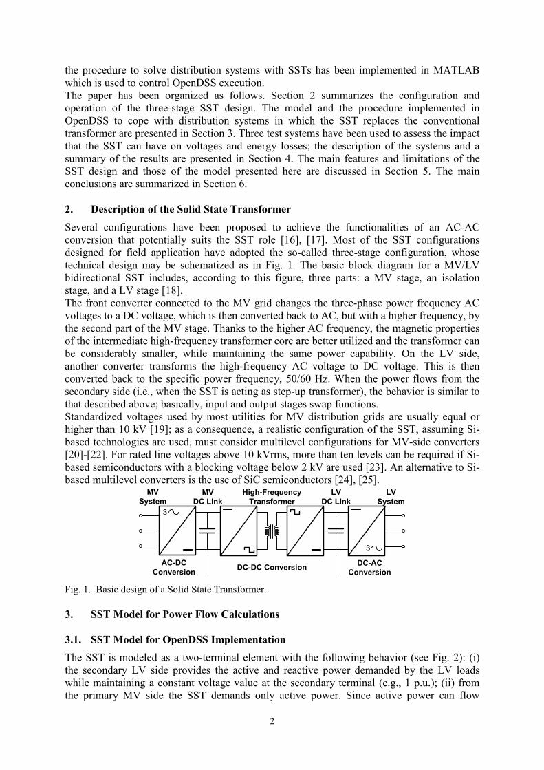
the procedure to solve distribution systems with SSTs has been implemented in MATLAB which is used to control OpenDSS execution. The paper has been organized as follows. Section 2 summarizes the configuration and operation of the three-stage SST design. The model and the procedure implemented in OpenDSS to cope with distribution systems in which the SST replaces the conventional transformer are presented in Section 3. Three test systems have been used to assess the impact that the SST can have on voltages and energy losses; the description of the systems and a summary of the results are presented in Section 4. The main features and limitations of the SST design and those of the model presented here are discussed in Section 5. The main conclusions are summarized in Section 6. 2. Description of the Solid State Transformer Several configurations have been proposed to achieve the functionalities of an AC-AC conversion that potentially suits the SST role [16], [17]. Most of the SST configurations designed for field application have adopted the so-called three-stage configuration, whose technical design may be schematized as in Fig. 1. The basic block diagram for a MV/LV bidirectional SST includes, according to this figure, three parts: a MV stage, an isolation stage, and a LV stage [18]. The front converter connected to the MV grid changes the three-phase power frequency AC voltages to a DC voltage, which is then converted back to AC, but with a higher frequency, by the second part of the MV stage. Thanks to the higher AC frequency, the magnetic properties of the intermediate high-frequency transformer core are better utilized and the transformer can be considerably smaller, while maintaining the same power capability. On the LV side, another converter transforms the high-frequency AC voltage to DC voltage. This is then converted back to the specific power frequency, 50/60 Hz. When the power flows from the secondary side (i.e., when the SST is acting as step-up transformer), the behavior is similar to that described above; basically, input and output stages swap functions. Standardized voltages used by most utilities for MV distribution grids are usually equal or higher than 10 kV [19]; as a consequence, a realistic configuration of the SST, assuming Si-based technologies are used, must consider multilevel configurations for MV-side converters [20]-[22]. For rated line voltages above 10 kVrms, more than ten levels can be required if Si-based semiconductors with a blocking voltage below 2 kV are used [23]. An alternative to Si-based multilevel converters is the use of SiC semiconductors [24], [25].

Fig. 1. Basic design of a Solid State Transformer. 3. SST Model for Power Flow Calculations 3.1. SST Model for OpenDSS Implementation The SST is modeled as a two-terminal element with the following behavior (see Fig. 2): (i) the secondary LV side provides the active and reactive power demanded by the LV loads while maintaining a constant voltage value at the secondary terminal (e.g., 1 p.u.); (ii) from the primary MV side the SST demands only active power. Since active power can flow

3

3

MV DC Link

LV DC Link

MVSystem

LVSystem

High-FrequencyTransformer

DC-DC Conversion DC-AC Conversion

AC-DC Conversion

3

through the SST in two directions, two operating modes are distinguished (see Fig. 2): Load and Generation modes. The models implemented in OpenDSS can be used to represent single- and three-phase bidirectional SSTs. They use two separate elements: LV voltage sources and MV loads, which will be respectively referred to as SST load and SST voltage source; Fig. 3 shows the diagram corresponding to a single-phase SST running in Load mode. The figure should be modified in case the SST operated in Generation mode: the direction of the arrows should then show active power flowing from the secondary side to the primary side.

Fig. 2. Schematic operation of the SST.

Fig. 3. SST model as implemented in OpenDSS (SST operates in Load mode). When the active power flows from the MV terminal to the LV terminal, the ideal SST voltage source provides all active and reactive power required by the LV loads and maintains a constant voltage value at its terminals for a load value below a certain level (see discussion at the end of this subsection and in Section 5). The load will replicate the SST behavior seen from the MV network: the active power demanded by the MV-side load will be equal to the active power served by the LV source plus the SST losses. In case of power flow reversal (i.e., the active power flows from the LV terminal to the MV terminal), the SST load becomes negative, so the MV SST terminal injects into the MV system the active power supplied from the LV terminal minus the SST losses. Under any of these conditions, the SST does not demand or inject any reactive power from the MV primary terminal: all reactive power demanded by loads is provided by the LV internal capacitor bank (see discussion at the end of this subsection). The basic relationships between active powers at both sides of the SST are, under the two operating modes, as follows:

0== PS

P QPPη

in Load Mode (1a)

0== PSP QPP η in Generation Mode (1b)

where PP and QP are respectively the active and reactive powers measured at the primary MV terminal of the SST, PS is the active power measured at the secondary LV terminal, and η is the SST efficiency.

P , Q

P + dP

Solid StateTransformer

(SST)

P , Q

P - dP

Solid StateTransformer

(SST)

Load mode

Generation mode

Medium Voltage(MV)

Low Voltage(LV)

Primary MVTerminal

Secondary LVTerminal

Load Voltage source

Solid State Transformer (SST)P + dP P + jQ

Controlledvoltage

4

Considering the current developments, the SST efficiency is lower than that of a conventional iron-and-copper transformer, unless SiC semiconductors were used [24], [25]. The presence of power converters introduces conduction and switching losses whose evaluation is not easy: power converter losses depend on the SST configuration and the strategies implemented to control the converters. Some work on SST losses and efficiency evaluation has been carried out to date; see [8], [9], [26]-[29]. Since it is assumed that the model implemented in OpenDSS includes MV and LV filters, loss calculations account also for filter losses. Fig. 4 shows the two efficiency curves used in this work: Option 1 corresponds to a rather realistic SST behavior (i.e., based on results presented in [26]), while Option 2 assumes a more optimistic behavior. Since SST efficiency exhibits some dependency on the load power factor [26], the following approach has been implemented in this work:

( ) ( ) ( )pfsfpfs αη ⋅=, (2)

where η is the efficiency curve for any load level, s, and any power factor, pf, while f(s) is the efficiency curve for a unity power factor, and depends on the load level (measured at the LV terminal):

ratedkVAkVAs = (3)

and α is a scale factor that depends on the power factor. In this work this function is given by:

( ) pfpf 02.098.0 +=α (4)

Fig. 4. SST efficiency. From the results presented in the literature, this approach is valid for load levels s above 5%; see [26]. On the other hand, not much information is available about SST efficiency for very low power factors (i.e., pf ≤ 0.1). However, loads below 5% and power factors close to zero can be present when power flow can reverse as a consequence of a high enough penetration of distributed generation (DG) in the network supplied from the secondary terminals of the SST. Based on efficiency studies presented in some works, see [26], [27], and on the extrapolation of results derived from the above formulae, the power loss surface, in per unit, shown in Fig. 5 was obtained. Note that this approach requires a full specification of losses such as that shown in Fig. 5. These losses can be obtained either from laboratory measurements or from simulations derived from a detailed model implemented in a time-domain simulation tool (e.g., an EMTP-type tool, MATLAB). However, this approach has some evident advantages: it is independent on the SST configuration and its control strategies, and it is already validated since the active

SST Load/Apparent Power (%)0 20 40 60 80 100

Effic

ienc

y (%

)

0

20

40

60

80

100

Option 1 Option 2

5

power flow in this model will be similar to that measured in the original SST prototype or model. The complete specification of a SST model for OpenDSS application includes the following items: • Rated power. • Rated voltages. • Efficiency curves or power losses (see Fig. 5) as function of the power and the power

factor. It is assumed the loss surface as that shown in Fig. 5 comes from either laboratory measurements or simulation results obtained with a detailed time-domain SST model.

• Limits for primary voltage (MV-side). Although this voltage is not controlled from the SST, the secondary LV side of the SST can correctly operate in case of voltage sag at the primary MV side [13]. However, it must be assumed that below certain voltage values the SST cannot correctly perform; therefore, the SST specification might include the maximum sag severity under which the LV stage of the SST will correctly operate. Although the implemented model can cope with this type of events, the SST operation under voltage sags has not been analyzed in this work.

• Control of secondary voltage (LV side). The SST can control this voltage so the model can be implemented to accept a voltage value that is estimated taking into account the state of the LV system supplied from the SST.

• Limits for the active and reactive powers at both SST sides. Since a bidirectional opera-tion is assumed, it can be also assumed that the limits for both active and reactive powers are the same at both SST sides. There are, however, some aspects to be considered. o The reactive power measured at the MV terminal of the implemented model is by

default zero in the case studies analysed in this paper, although the SST can be designed to support MV system voltage by injecting reactive power into the MV distribution system. Since the reactive power flows measured at both terminals are fully decoupled, the limits for reactive power can be different at both sides in case the primary side of the SST was used to support the MV network. See Discussion included in Section 5.

o LV side overload is an operating condition that should be accounted for. Although it can be assumed that the model implemented for this work can cope with certain overload level, it will obviously fail to keep secondary side voltage at the desired value if the overload is too high. This aspect is also discussed in Section 5.

Fig. 5. SST losses – Option 1 in Fig. 4.

3.2. Power Flow Solution with SST Model

Power FactorPower (p.u.)

Pow

er L

osse

s (p

.u.)

1.00.80.60.40.20.01.00.80.60.40.2

0.15

0.10

0.05

0.000.0

6

The procedure implemented in MATLAB-OpenDSS to obtain a load flow solution when at least one SST is included in the system model may be summarized as follows:

1. Solve the system using initial “dummy” values for the SST loads (see Fig. 3); the initial values can also be inherited from a previous solution. These initial values will not interfere with the loads connected to the secondary terminal of the SST, as they are independently served by the SST voltage source.

2. Read the total active and reactive power provided by the SST voltage source. 3. Calculate the power demanded by the SST from the MV network by adding losses. 4. Update power values for the SST loads. 5. Solve the system with correct values.

If the system solution is required as a function of time, this procedure is repeated for every time step. Fig. 6 shows a flow chart of the procedure assuming a time-driven simulation.

Fig. 6 Flow chart of the power flow solution implemented in OpenDSS. As for the procedure, it is worth keeping in mind the following aspects: • The use of dummy values for SST loads in step 1 is aimed at making the OpenDSS

solution process as direct as possible. This approach allows implementing and using the SST model without having to extensively modify an already existing system. With this solution process, it is only necessary to remove the conventional transformer (by disabling or deleting it from the system) and replace it by defining two new elements (the SST load and the SST voltage source). The proposed procedure is able to simulate the system with SSTs by simply specifying a flag for both elements (so the procedure can recognize them as part of the SST model).

• The three-phase model of the SST is composed by a three-phase voltage source (SST voltage source) and a three-phase balanced load (SST load), where the SST load is modeled as a PQ load. In step 2 the procedure reads the total active and reactive power provided by the SST voltage source and then proceeds to calculate the power demanded from the MV network by adding losses. Step 3 is performed without considering the

Define Load object connected to MV bus

YES

Define Vsource object connected to LV bus

Solve system using Load initial value

Calculate power delivered by Vsource object

Add losses to power delivered by Vsource object

Solve system using Load new value

Is simulation finished?

End

Advance simulation one time step NO

Solve system using Load present value

7

power supplied by each individual phase of the SST voltage source; that is, the power to be demanded by the SST from the MV network is calculated taking only into account the total power served by the SST voltage source. In step 4 the power values for the SST loads are updated, since the SST load is a three-phase balanced load, the power consumed will be equally distributed among the three phases. By using a three-phase balanced load to represent the behavior of the SST from the MV side, the model will always demand balanced power from the MV network regardless of the unbalance present in the LV network served by the SST. In other words, both the primary and the secondary of the SST model can be connected to either balanced or unbalanced systems. The solution at both sides is provided by the OpenDSS engine; however, the only information passed from one SST side to the other is the active power plus/minus (depending on the active power flow direction) losses.

4. Case Studies Three distribution system models are used to test the performance of the SST model implemented in MATLAB-OpenDSS. The first system has been edited on purpose for this work and simulated in snapshot mode. The other two test systems are based on system models supplied with OpenDSS; each one has been tested considering different time periods and operating conditions, and with load curves supplied with OpenDSS, while generation curve shapes were derived with a procedure developed by the authors [30]. 4.1. Test System 1 The 50 Hz overhead test system depicted in Fig. 7 feeds two loads from transformers with the same ratings (11/0.416 kV, 100 kVA), being the short-circuit reactance and the ratio X/R for both transformers 6% and 8, respectively. The rated power of the substation transformer is 250 kVA. The voltage of the HV source that feeds the system remains constant at 1.05 p.u. The distances between the substation and the two loads are 10 km. The two loads are represented by a ZIP model; each part of the load model has been assigned a weighting factor equal to 1/3 for both active and reactive powers.

Fig. 7. Configuration of Test System 1. The system has been simulated when one or the two conventional transformers are replaced by SSTs of the same ratings. The efficiency of SSTs is according Option 2 in Fig. 4 and specified by means of the power loss surface, see Fig. 5. Table I summarizes the main results. Although the efficiency of conventional transformers is about 98.5% and SST losses are larger than their conventional counterpart, SSTs exhibit a good enough performance that is favored by two SST capabilities: (i) since voltages at the secondary terminals of SSTs are controlled to 1 p.u., load voltages improve when SSTs are installed; (ii) system losses decrease due to the reactive power compensation provided from the MV side of SSTs, as a consequence some power release in the substation transformer is also achieved. Note that

TR2

TR1

230 kV 11 kV

11 kV 0.416 kV

90 kVApf = 0.8 (lg)

90 kVApf = 0.8 (lg)

1 2

3

4

HV system

8

when SSTs are used, the efficiency is lower and the power measured at the MV side of the substation is higher; this is caused by the combination of larger SST losses and the increase of the LV load powers due to the voltage improvement provided by SSTs. Remember that loads are voltage dependent.

Table I – Test System 1 – Simulation results

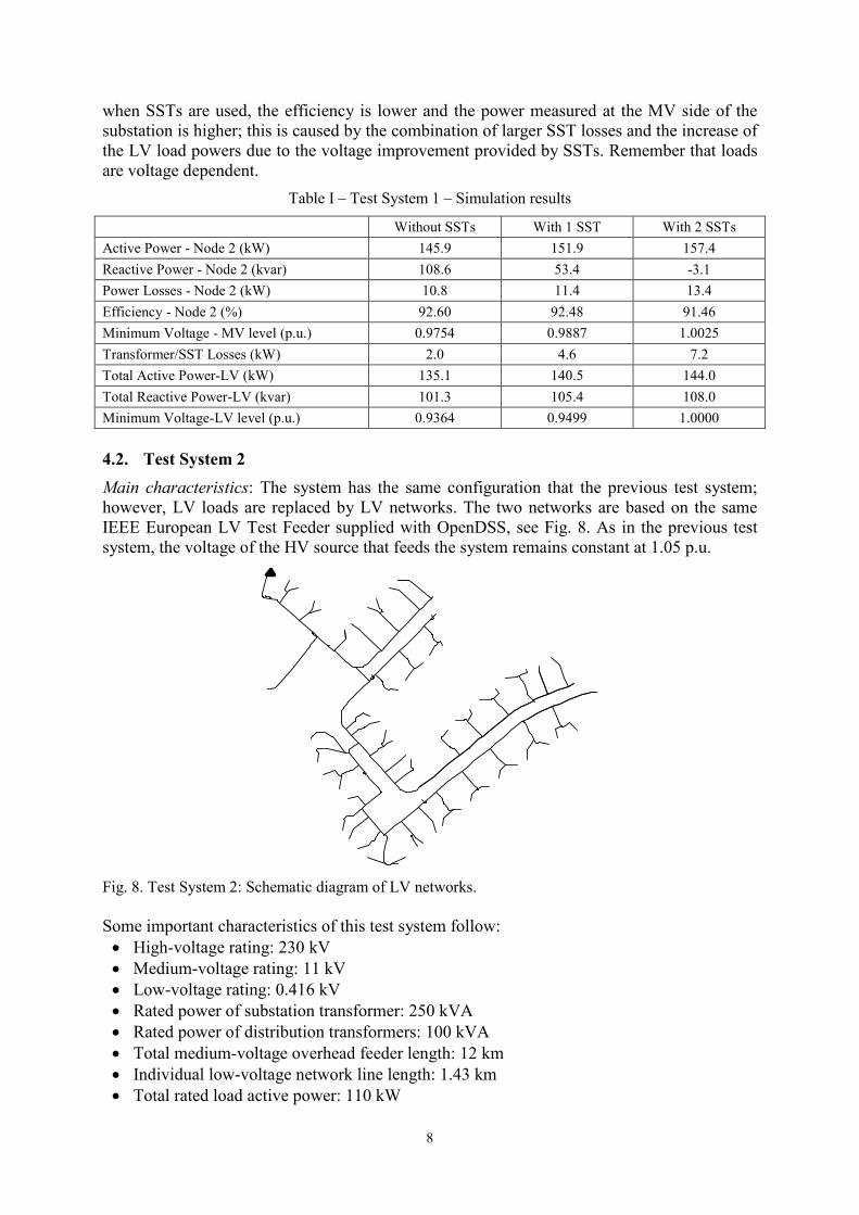
Without SSTs With 1 SST With 2 SSTs Active Power - Node 2 (kW) 145.9 151.9 157.4 Reactive Power - Node 2 (kvar) 108.6 53.4 -3.1 Power Losses - Node 2 (kW) 10.8 11.4 13.4 Efficiency - Node 2 (%) 92.60 92.48 91.46 Minimum Voltage - MV level (p.u.) 0.9754 0.9887 1.0025 Transformer/SST Losses (kW) 2.0 4.6 7.2 Total Active Power-LV (kW) 135.1 140.5 144.0 Total Reactive Power-LV (kvar) 101.3 105.4 108.0 Minimum Voltage-LV level (p.u.) 0.9364 0.9499 1.0000 4.2. Test System 2 Main characteristics: The system has the same configuration that the previous test system; however, LV loads are replaced by LV networks. The two networks are based on the same IEEE European LV Test Feeder supplied with OpenDSS, see Fig. 8. As in the previous test system, the voltage of the HV source that feeds the system remains constant at 1.05 p.u.

Fig. 8. Test System 2: Schematic diagram of LV networks. Some important characteristics of this test system follow: • High-voltage rating: 230 kV • Medium-voltage rating: 11 kV • Low-voltage rating: 0.416 kV • Rated power of substation transformer: 250 kVA • Rated power of distribution transformers: 100 kVA • Total medium-voltage overhead feeder length: 12 km • Individual low-voltage network line length: 1.43 km • Total rated load active power: 110 kW

9

• Total rated load reactive power: 44.37 kvar • Total number of LV loads: 110.

Loads have been represented again by the ZIP model with the same characteristics that in the previous study. The same group of load shapes has been used in all LV networks; this means a coincidence factor of 1 between LV feeders, which can increase the load at the MV substation terminals, and therefore the voltage drop at MV and LV nodes. Simulation results: The goal is to analyze the impact of the SST by comparing the system behavior when transformer TR2 is replaced by a SST and photovoltaic (PV) generation is connected to the LV network supplied from that transformer. In this study, the system performance is analyzed during a 24-hour period. Since the SST can react to load and voltage changes in a few power-frequency cycles, the test system is simulated using a 1-minute time step. PV generators connected to LV networks only inject active power, being the total rated power of PV generators about 40% of the rated power of distribution transformers. Results are summarized in Table II. Fig. 9 shows some simulation results obtained with a SST efficiency that corresponds to Option 1 in Fig. 4. The following conclusions can be derived from these results: • The coincidence among load profiles causes large voltage drops at LV nodes during load

peaks (see Fig. 9c), although values above 1 p.u. are obtained during some periods at both MV and LV levels. The increase of voltage in the MV system above 1 p.u. is exacerbated when PV generation is connected to LV networks and the load is served from conventional transformers only. Some type of measure is required when conventional transformers are used since voltages can reach both too high and too low values. A better performance is obtained when the SST is installed; variations in MV voltage values are then smaller.

Table II – Test System 2 – Simulation results

Without DG With DG

Without SSTs

One SST Without SSTs

One SST Opt. 1 Opt. 2 Opt. 1 Opt. 2 Active Energy - MV side of substation (kWh) 1070.6 1187.0 1114.5 887.4 969.1 914.8 Reactive Energy - MV side of substation (kvarh) 340.0 124.2 124.1 337.3 123.9 123.8 Energy Losses - MV side of substation (kWh) 52.7 176.4 103.4 47.4 137.8 83.2 Efficiency - MV side of substation (%) 95.08 85.14 90.72 95.57 88.02 92.41 Maximum Power - MV side of substation (kW) 123.0 133.2 127.9 101.1 109.6 104.8 Maximum Voltage - MV level (p.u.) 1.0502 1.0504 1.0504 1.0533 1.0517 1.0527 Minimum Voltage - MV level (p.u.) 0.9863 0.9957 0.9973 0.9937 1.0035 1.0047 Energy served by Transformers/SSTs - LV side (kWh) 1028.9 1021.6 1022.1 860.3 853.0 853.4

Reverse Energy Flow through Transformers - LV side (kWh) ----- ----- ----- 10.5 12.0 12.0

Total Transformer/SST Energy Losses (kWh) 23.2 146.1 75.2 22.8 113.6 60.3 Active Energy Supplied to LV loads (kWh) 1017.9 1010.6 1011.1 1021.8 1013.1 1013.5 Active Energy Supplied by PV Generators – LV level (kWh) ----- ----- ----- 181.8 181.8 181.8

Total Energy Losses in LV Networks (kWh) 11.0 11.0 11.0 9.8 9.8 9.8 Maximum Voltage - LV level TR1 (p.u.) 1.0484 1.0483 1.0486 1.0561 1.0514 1.0520 Minimum Voltage - LV level TR1 (p.u.) 0.8789 0.8945 0.8959 0.8862 0.9022 0.9032 Maximum Voltage - LV level TR2/SST (p.u.) 1.0484 1.0166 1.0166 1.0662 1.0237 1.0237 Minimum Voltage - LV level TR2/SST (p.u.) 0.8775 0.9318 0.9318 0.8954 0.9389 0.9389

10

a) Active power measured at the MV substation terminal

b) Reactive power measured at the MV substation terminal

c) Minimum voltage at LV levels Fig. 9. Test System 2 – Simulation results – Option 1 (see Fig. 4). • As expected, SST energy losses depend on the efficiency curve; they are higher with

Option 1 and lower with Option 2 (see Fig. 4). The lowest losses in the MV distribution system occur with one SST and Option 2 due to the reactive power compensation it provides at the MV terminals. Losses in LV networks are very similar, although they decrease when PV generation is connected. The combination of these effects increases the active energy that must be supplied from the substation when one SST is installed.

• When one SST is operating, reactive power at the MV level is compensated and a reduction is noticed at the substation terminals. In turn, the active energy served from the substation with respect to that required without the SST depends on the SST efficiency.

During some periods of the day, PV generation causes power flow reversal through the SST, which allows LV generation surplus be injected into the MV network. The operation principle for the SST remains the same when working under reverse power flow: the power injected into the MV network will be equal to the generation surplus received on the secondary terminal minus the SST losses (see Fig. 2 and equation (1b)), and the SST efficiency is the same as under load-mode operation. 4.3. Test System 3 Main characteristics: Fig. 10 shows the one-line diagram of EPRI Circuit 7 used as test system in the new study. It is a 60 Hz system that serves a mixture of single- and three-phase loads connected at different rated voltages (12.47, 0.24, and 0.208 kV). The model includes a simplified representation of the HV system and the substation, which is composed by three

Without STTWith STT

Hour0 4 8 12 16 20 24

Act

ive

Pow

er (k

W)

-50

0

100

50

150

Hour0 4 8 12 16 20 24

Rea

ctiv

e Po

wer

(kva

r)

-20

0

40

20

60Without STTWith STT

Without STTWith STT

Hour0 4 8 12 16 20 24

Volta

ge (p

.u.)

0.85

1.00

1.05

0.95

0.90

11

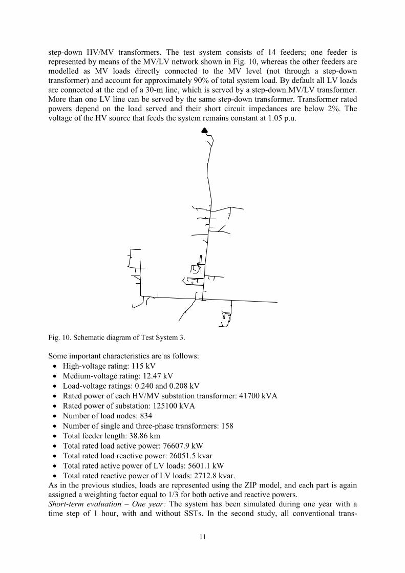
step-down HV/MV transformers. The test system consists of 14 feeders; one feeder is represented by means of the MV/LV network shown in Fig. 10, whereas the other feeders are modelled as MV loads directly connected to the MV level (not through a step-down transformer) and account for approximately 90% of total system load. By default all LV loads are connected at the end of a 30-m line, which is served by a step-down MV/LV transformer. More than one LV line can be served by the same step-down transformer. Transformer rated powers depend on the load served and their short circuit impedances are below 2%. The voltage of the HV source that feeds the system remains constant at 1.05 p.u.

Fig. 10. Schematic diagram of Test System 3. Some important characteristics are as follows: • High-voltage rating: 115 kV • Medium-voltage rating: 12.47 kV • Load-voltage ratings: 0.240 and 0.208 kV • Rated power of each HV/MV substation transformer: 41700 kVA • Rated power of substation: 125100 kVA • Number of load nodes: 834 • Number of single and three-phase transformers: 158 • Total feeder length: 38.86 km • Total rated load active power: 76607.9 kW • Total rated load reactive power: 26051.5 kvar • Total rated active power of LV loads: 5601.1 kW • Total rated reactive power of LV loads: 2712.8 kvar.

As in the previous studies, loads are represented using the ZIP model, and each part is again assigned a weighting factor equal to 1/3 for both active and reactive powers. Short-term evaluation – One year: The system has been simulated during one year with a time step of 1 hour, with and without SSTs. In the second study, all conventional trans-

12

formers are replaced by SSTs. Since most conventional transformers are oversized, two different scenarios were considered: in the first one, all conventional transformers were replaced by SSTs of the same ratings (i.e., same rated power and voltages); in the second scenario, when it was possible, the rated power of SSTs was lower than that of the corresponding conventional transformer. The steps used to fix the reduced SST ratings were as follows: (i) a long term simulation, as detailed below, was carried out with only conventional transformers and considering their original ratings; (ii) the peak power supplied by each transformer (in kVA) was obtained; (iii) the reduced SST ratings were derived by increasing those peak power values by a 15% security margin. The final values were rounded-up in steps of 5 kVA. This reduction was applied to a total of 141 SSTs. Table III provides some results obtained from one-year evaluation. Fig. 11 presents some simulation results; all results are presented for the same time period when the SST efficiency corresponds to Option 1 in Fig. 4 and SST rated powers are equal to those of the conventional transformers they replace.

Table III – Test system 3 – Simulation results Short Term Evaluation - One Year

Variable Without SSTs

With SSTs Original Rated Powers Reduced Rated Powers

Option 1 Option 2 Option 1 Option 2 Active Energy - MV side of substation (MWh) 275455.6 284107.8 279545.7 281047.4 277871.4 Reactive Energy - MV side of substation (Mvarh) 85558.5 76674.7 77448.5 77323.7 78372.1

Total Energy Losses - MV side of substation (MWh) 998.1 9282.2 4723.8 6231.2 3087.9

Efficiency (without substation losses) (%) 99.64 96.73 98.31 97.78 98.89 Maximum Power - MV side of substation (kW) 66704.9 67979.2 67476.5 67663.2 67310.4

Minimum Voltage - MV level (p.u.) 0.9688 0.9787 0.9779 0.9775 0.9787 Active Energy served by Transformers/SSTs - MV side (MWh) 28448.2 36423.9 31949.7 33432.0 30344.4

Total Transformer Energy Losses (MWh) 529.2 8665.7 4191.4 5673.8 2586.1 Active Energy served by Transformers/SSTs - LV side (MWh) 27919.0 27758.2 27758.2 27758.2 27758.2

Minimum Voltage - LV level (p.u.) 0.9155 0.9405 0.9405 0.9405 0.9405 Long Term Evaluation – Ten Years

Variable Without SSTs

With SSTs Original Rated Powers Reduced Rated Powers

Option 1 Option 2 Option 1 Option 2 Active Energy - MV side of substation (MWh) 2993449.8 3087238.8 3039244.6 3055071.2 3022054.6 Reactive Energy - MV side of substation (Mvarh) 933912.4 809106.2 823473.3 818300.3 829321.6

Total Energy Losses - MV side of substation (MWh) 10793.9 97051.9 49371.7 65068.4 32348.3

Efficiency (without substation losses) (%) 99.64 96.86 98.38 97.87 98.93 Maximum Power - MV side of substation (kW) 78796.5 80333.4 79790.6 79979.4 79602.0 Minimum Voltage - MV level (p.u.) 0.9474 0.9596 0.9623 0.9614 0.9631 Total Energy served by Transformers/SSTs - MV side (MWh) 309430.2 393519.2 346812.8 362210.3 330116.0

Total Transformer Energy Losses (MWh) 5381.8 89853.4 43147.0 58544.6 26450.3 Active Energy served by Transformers/SSTs - LV side (MWh) 304048.4 303665.8 303665.8 303665.8 303665.8

Minimum Voltage - LV level (p.u.) 0.8960 0.9405 0.9405 0.9405 0.9405

13

a) Active powers measured at the MV terminal of the substation

b) Reactive powers measured at the MV terminal of the substation

c) Voltage at the MV terminal of transformer 1001577

d) Voltage at the LV terminal of transformer 1001577 Fig. 11. Test System 3 – Simulation results – Option 1 (see Fig. 4). Differences are not significant, except for voltages at LV sections. The active energy measured at any terminal of the substation transformers is higher and the reactive energy is lower with SSTs. According to Figs. 11c and 11d, which show the variation of the minimum voltage at the two terminals of one transformer, voltages do not experience any significant variation at MV levels, and during low load periods voltages at both MV and LV levels can reach values higher than 1 p.u. Remember that the voltage at the HV terminals of the substation remains constant at 1.05 p.u. The results provided in Table III show a rise in both the energy losses and the active power to be supplied from the substation when conventional transformers are replaced by SSTs. The increase of SSTs losses exceeds the reactive power compensation effect provided by the MV side of SSTs in the MV-level system. An increase of the active energy is also caused by the voltage dependency of loads, which increases active load with voltage. In this system the

Hour1008 1032 1056 1080 1104 1128 1152984

Act

ive

Pow

er (M

W)

20

30

40

50

60Without STTWith STT

Hour1008 1032 1056 1080 1104 1128 1152984

Rea

ctiv

e Po

wer

(Mva

r)

5

10

15

20Without STTWith STT

Hour1008 1032 1056 1080 1104 1128 1152984

Volta

ge (p

.u.)

0.98

1.00

1.02

1.04Without STTWith STT

Hour1008 1032 1056 1080 1104 1128 1152984

Volta

ge (p

.u.)

0.97

0.99

1.00

1.01

1.02

0.98 Without STTWith STT

14

energy served from LV terminals is lower with SSTs than with conventional transformers, whereas the energy directly served from MV nodes to some large loads increases. The combination of all these effects causes an increase of active energy and a decrease of reactive energy at both HV and MV terminals of the substation. As expected, the best SST performance is achieved when the SST efficiency corresponds to Option 2 in Fig. 4 and SST sizes are smaller than those assumed in the original test system model. Although all step-down conventional transformers are oversized, the voltage at LV levels decreases to values as low as 0.9155 pu (see Table III). When all these transformers are replaced by SSTs, the power flows across the new transformers are rather low and so is the efficiency (see Fig. 4). The table shows other expected results: the efficiency of SSTs increases when their rated powers are decreased; this also affects energy losses and the required active energy, being both lower. Note that efficiencies are rather high even when SSTs replace conventional transformers. This behavior is due to the fact that in the system model the load served from MV/LV transformers or SSTs is rather small compared to the full system load. Long-term evaluation – Ten years: Since the SST efficiency increases with the load level (see Fig. 4), a second study has been carried out to evaluate the system after a period of 10 years during which the average growth of nominal loads was that depicted in Fig. 12. The new results are also shown in Table III. An obvious conclusion is that some type of measure is required when conventional transformers are used, since during the period covered by the study the voltage at some LV sections would be unacceptable. As expected, minimum voltage values at both MV and LV levels are lower than those obtained from the previous evaluation with conventional transformers. The minimum voltage at LV levels with SSTs is the same in both studies (i.e., 0.9405 pu); it corresponds to a load whose rated power remains constant during the 10-year period. Its value was initially high and caused the maximum voltage drop at LV levels during the first year. On the other hand, the overall efficiency for each case study with SSTs has slightly increased during the 10-year period; this is due to the comparatively lower active energy at the MV level caused by a decrease of MV-level voltages and the better SST efficiency.

Fig. 12. Test System 3 - Growth of nominal load. 5. Discussion

• SST vs. conventional transformer: The SST and the conventional transformer share some functions, but the SST is capable of providing additional ancillary services, such as voltage regulation and reactive power compensation. However, the technology behind the SST is not as mature as the conventional transformer’s: current SST designs present efficiencies lower than those of conventional transformers and a life cycle shorter than their iron-and-copper counterpart [3]. Moreover, the large number of elements that compose the SST (semi-conductors, high-frequency transformer, control circuits, filters) will have an impact on its reliability [3]. It is expected that technology advances applied to the SST will help to improve its efficiency and reliability, thus closing the gap with respect to the conventional transformer.

Year1 2 3 4 5 6 7 8 9 10

Cum

mul

ativ

e Lo

ad

Gro

wth

(%)

0

0.05

0.10

0.15

0.20

0.25

15

• SST response: The proposed SST model is adequate for power flow calculations as it includes features to be considered in planning studies (e.g., secondary side voltage control, reactive power compensation, MV load balancing, SST efficiency). Although additional control strategies can be easily implemented into the developed model, it is important to keep in mind some important differences between the responses of a model for power flow calculations and a model implemented in a time-domain tool (e.g., EMTP or MATLAB). Time-domain SST models use a very short time step (e.g., in the order of 1 µs or less, see [11], [13]) and their solutions provide detailed SST behavior. Time steps used in time-driven quasi-static power flow simulations usually range from one minute to one hour, and their response in front of a control action cannot be included into the response of the model until the effect is finished.

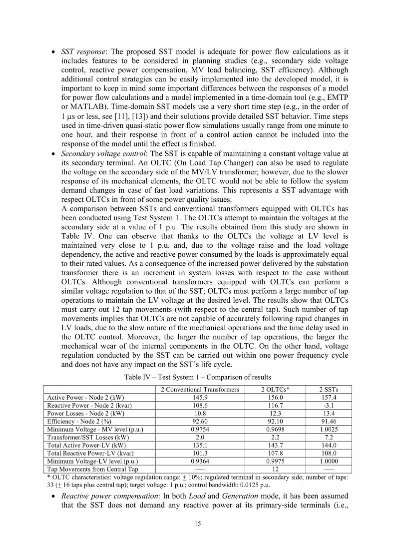
• Secondary voltage control: The SST is capable of maintaining a constant voltage value at its secondary terminal. An OLTC (On Load Tap Changer) can also be used to regulate the voltage on the secondary side of the MV/LV transformer; however, due to the slower response of its mechanical elements, the OLTC would not be able to follow the system demand changes in case of fast load variations. This represents a SST advantage with respect OLTCs in front of some power quality issues. A comparison between SSTs and conventional transformers equipped with OLTCs has been conducted using Test System 1. The OLTCs attempt to maintain the voltages at the secondary side at a value of 1 p.u. The results obtained from this study are shown in Table IV. One can observe that thanks to the OLTCs the voltage at LV level is maintained very close to 1 p.u. and, due to the voltage raise and the load voltage dependency, the active and reactive power consumed by the loads is approximately equal to their rated values. As a consequence of the increased power delivered by the substation transformer there is an increment in system losses with respect to the case without OLTCs. Although conventional transformers equipped with OLTCs can perform a similar voltage regulation to that of the SST; OLTCs must perform a large number of tap operations to maintain the LV voltage at the desired level. The results show that OLTCs must carry out 12 tap movements (with respect to the central tap). Such number of tap movements implies that OLTCs are not capable of accurately following rapid changes in LV loads, due to the slow nature of the mechanical operations and the time delay used in the OLTC control. Moreover, the larger the number of tap operations, the larger the mechanical wear of the internal components in the OLTC. On the other hand, voltage regulation conducted by the SST can be carried out within one power frequency cycle and does not have any impact on the SST’s life cycle.

Table IV – Test System 1 – Comparison of results 2 Conventional Transformers 2 OLTCs* 2 SSTs

Active Power - Node 2 (kW) 145.9 156.0 157.4 Reactive Power - Node 2 (kvar) 108.6 116.7 -3.1 Power Losses - Node 2 (kW) 10.8 12.3 13.4 Efficiency - Node 2 (%) 92.60 92.10 91.46 Minimum Voltage - MV level (p.u.) 0.9754 0.9698 1.0025 Transformer/SST Losses (kW) 2.0 2.2 7.2 Total Active Power-LV (kW) 135.1 143.7 144.0 Total Reactive Power-LV (kvar) 101.3 107.8 108.0 Minimum Voltage-LV level (p.u.) 0.9364 0.9975 1.0000 Tap Movements from Central Tap ----- 12 ----- * OLTC characteristics: voltage regulation range: + 10%; regulated terminal in secondary side; number of taps: 33 (+ 16 taps plus central tap); target voltage: 1 p.u.; control bandwidth: 0.0125 p.u.

• Reactive power compensation: In both Load and Generation mode, it has been assumed that the SST does not demand any reactive power at its primary-side terminals (i.e.,

16

reactive power consumed by loads in the LV network served by the SST is provided by the LV internal capacitor bank). However, SST capabilities can also be used to support MV network voltages, as well as reducing losses and overall system loading, by injecting reactive power into the grid. The development of a control algorithm that estimates the amount of reactive power that should be injected from the primary side based on the operating conditions of the MV network and the SST itself is out of the scope of this paper; however, the changes required in the model proposed here to analyze the response of such algorithms are minimum; all that is necessary is to update both active and reactive power values of the SST load in step 4 of the solution process. This action is very straightforward and represents another advantage of the presented SST model.

• SST model validation: Time-domain SST models (i.e., EMTP- or MATLAB-based models) are detailed models that can accurately predict the response of the SST under steady state and transient conditions [11], [13]. For steady-state simulations those models and that presented here should provide similar behaviors. Obviously, a model for power flow calculations cannot replicate the behavior of the SST under transient conditions. In any case, it is reasonable to think that a model for power flow calculations could be validated by comparing results from power flow calculations with those derived from a detailed time-domain model running under steady state conditions. One aspect of the proposed model that requires special attention is the representation of losses. Although there are several works that address this issue [26] - [29], to date a complete time-domain model capable of accurately predicting SST losses for all operating conditions (including Load and Generation mode) has not been presented; SST losses are highly dependent on the SST configuration and switching strategies of the semiconductors. Therefore, the objective of this work is to present a general power flow model that could represent any SST configuration including losses (based on existing works) and could be easily adapted to any new findings in this field. That is, the representation of losses as depicted in Fig. 4 or Fig. 5 is as general as possible and can be easily adapted to any SST design.

• SST operation under overload conditions: The SST rated power can be defined as the maximum power (served from the secondary side) with which the SST is capable of maintaining secondary-side voltage and frequency values. None of the SSTs experienced overload in the studies carried out with the test systems used in the present paper; namely all SSTs served a load (in kVA) lower than its rated power. However, the SST behavior when serving a load greater than its rated power is a subject that must be addressed. Under overload conditions the SST may fail to operate according to design specifications; being the controlled voltage on the secondary side the greatest concern in power flow studies. Two different approaches could be used to face this issue. o Voltage source with series impedance: For loads equal or below the SST rated

power the value of the series impedance is assumed negligible. However, for loads above the rated power the value of this impedance can be modified in order to account for SST inability to achieve the desired voltage value at its secondary terminal. The impedance value should be calibrated to obtain the desired voltage drop for specific loading conditions.

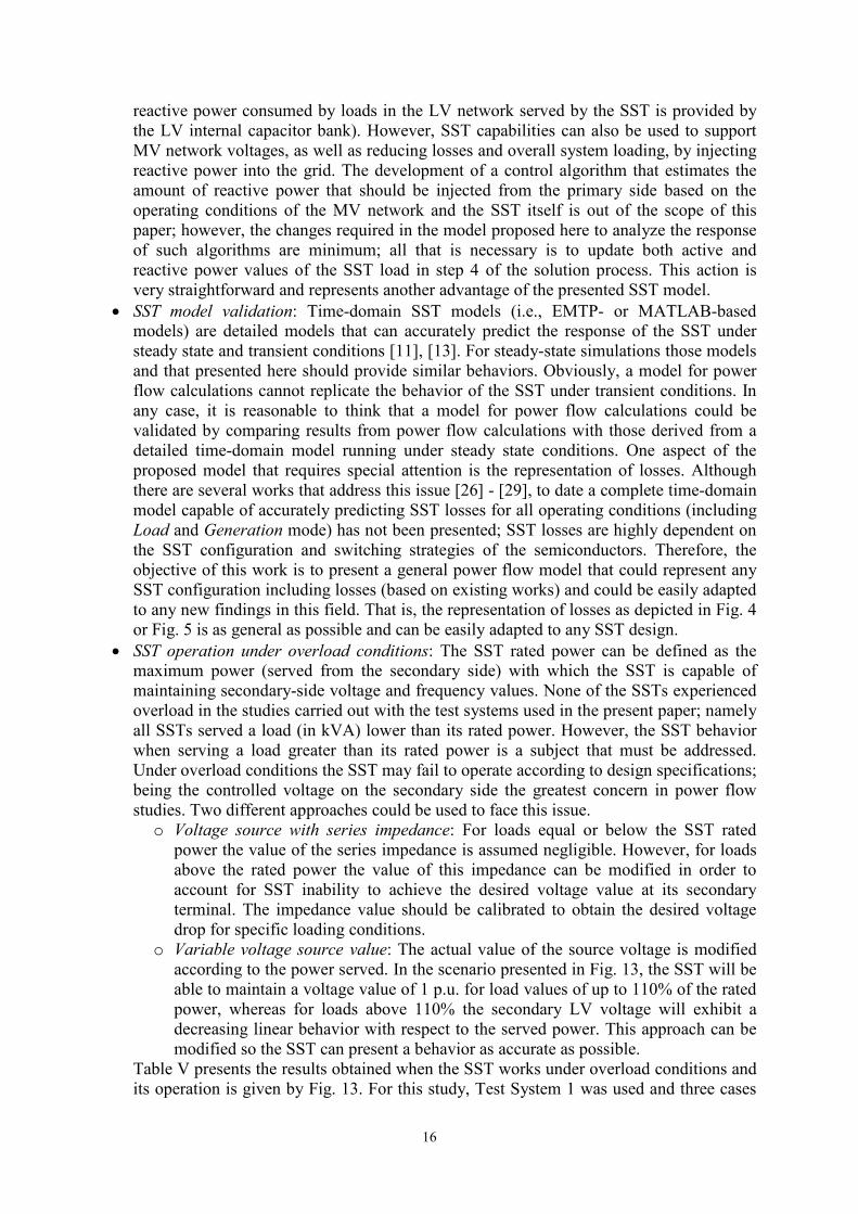
o Variable voltage source value: The actual value of the source voltage is modified according to the power served. In the scenario presented in Fig. 13, the SST will be able to maintain a voltage value of 1 p.u. for load values of up to 110% of the rated power, whereas for loads above 110% the secondary LV voltage will exhibit a decreasing linear behavior with respect to the served power. This approach can be modified so the SST can present a behavior as accurate as possible.

Table V presents the results obtained when the SST works under overload conditions and its operation is given by Fig. 13. For this study, Test System 1 was used and three cases

17

were evaluated: (i) the load in both transformers is 90% of the SST’s rated power (original case in Section 4.1), (ii) the rated load connected to TR2 is increased to 115% of the rated power, and (iii) the rated load is set to 130%. In all cases the load power factor is 0.8 (lg) and Option 2 is used for the SST efficiency. From these results, it can be noted that the minimum voltage at LV level is no longer equal to 1 p.u. when the load is above 110% of the SST’s rated power and the actual powers served by the SST differ from rated values due to the voltage dependency of loads.

Fig. 13. SST response in front of an overload.

Table V – Test System 1 – Simulation results with overloads

With conventional transformers With SSTs Case 1 Case 2 Case 3 Case 1 Case 2 Case 3

Active Power - Node 2 (kW) 145.9 165.1 176.4 157.4 177.9 186.0 Reactive Power - Node 2 (kvar) 108.6 124.2 133.6 -3.1 -2.8 -2.7 Power Losses - Node 2 (kW) 10.8 13.9 15.9 13.4 15.3 16.1 Efficiency - Node 2 (%) 92.60 91.61 90.97 91.46 91.39 91.33 Minimum Voltage - MV level (p.u.) 0.9754 0.9642 0.9575 1.0025 0.9954 0.9926 Transformer/SST Losses (kW) 2.0 2.4 2.7 7.2 7.4 7.4 Total Active Power-LV (kW) 135.1 151.2 160.5 144.0 162.6 169.8 Total Reactive Power-LV (kvar) 101.3 113.4 120.4 108.0 121.9 127.4 Minimum Voltage-LV level (p.u.) 0.9364 0.9140 0.9005 1.0000 0.9846 0.9395

• Current balance: One important SST feature is the possibility of balancing currents

and/or powers. The isolation stage of the design shown in Fig. 1 decouples input and output stages, and can be used to obtain balanced powers/currents at the MV side when the powers/currents are not balanced at the LV side. Fig. 14 depicts some results obtained from the simulation of Test System 2 in which the SST supplies three unbalanced LV loads; according to the plots shown in the figure, the active powers measured at the MV terminals are balanced (i.e., there is a full match of the power measured at each MV terminal) while the powers measured at each LV terminal are different.

• DC supply: SST secondary terminals can also be used as DC source or AC source with an output frequency different from power frequency [3]-[13]. The implementation of a SST with a LV DC supply in the present model is straightforward. This approach can be easily extended to SSTs with either one or three-phases at the MV side, considering the two approaches mentioned above for representing the DC source voltage (i.e., with either a variable voltage value or a series impedance). Note that a SST used only for supplying DC voltage would be a simplified version of the device shown in Fig. 1; this would have some impact on the SST losses since neither the secondary converter not the LV output filter would be included in the design.

SST Load/Apparent Power (%)0 30 60 90 120 150C

ontr

olle

d Vo

ltage

(p.u

.)

0.80

0.85

0.90

0.95

1.00

1.05

18

Fig. 14. Test System 2 – Simulation results with unbalanced loads. • Harmonic propagation: The SST design presented in Fig. 1 exhibits some important

features that can be used to face some power quality problems; see Introduction. Among other advantages, the SST can prevent the propagation of harmonic currents from the LV side to the MV side; this is another consequence of implementing the isolation stage as a DC-DC converter (see illustrative examples presented in [11] and [13]). Although OpenDSS has capabilities for harmonic analysis (e.g., frequency scan), it does not allow mixing sources of different frequencies in the same case so the application to cases in which nonlinear loads are connected to the LV system is rather limited. In addition, there is another important aspect to be accounted for: the user needs some information about the SST efficiency when the secondary currents are not sinusoidal since losses will be different from those caused with purely sinusoidal currents.

6. Conclusions The SST is a versatile device that can provide new power quality solutions to the future smart grid. This paper has presented a SST model for OpenDSS implementation. This model can be used to explore and assess the impact of the SST on distribution system performance (i.e., in steady-state power flow calculations) considering either a short- or long-term evaluation. From the results presented in this paper, it is evident that the SST efficiency is one of the main drawbacks. An important aspect to be considered when the efficiencies of the conventional transformer and the SST are compared is that the information that matters is the energy loss obtained with each device during the period of interest. Given the dependency of the SST efficiency with respect to the load level and power factor, one should expect that the energy losses in the system under study when the SST replaces one or more conventional transformers will be higher than those obtained with conventional transformers during periods with low load level; however, in some case studies they could be lower during periods with high load levels, due also to the reactive power compensation provided by the SST at the MV side. At the end the quantities to be compared are the long-term energy losses obtained with both devices (e.g., during periods equal or longer than one year), although considering the current achievements very rarely the efficiency obtained with SSTs will be better than that obtained with conventional transformers. Voltage control provided from the SST LV terminals can be used to both increase and decrease voltage, which will also affect the energy to be supplied to loads. Since SST capabilities can be used to perform voltage control in both directions, SST can simultaneously optimize the voltage and the energy required by loads. Obviously, voltage control of LV networks can also be achieved by using tapped conventional transformers; the advantage of

Hour0 4 8 12 16 20 24

0

10

20

30

40Po

wer

(kW

)

0

10

20

30

40

Pow

er (k

W) MV Terminals

LV Terminals

Phase APhase BPhase C

Phase APhase BPhase C

19

the SSTs is its fast response: it can react to voltage variations in a few power-frequency cycles. In addition, the reactive power compensation provided from the MV terminal can be used to reduce energy losses and control voltage at MV levels. The results presented in this paper should be used with care. Taking into account all potential SST capabilities, the strategies to be considered when a conventional transformer is replaced by a SST could be different from those analyzed here. The SST model, as simulated in this paper, injects/ absorbs only active power from its MV terminal and maintains constant the LV terminal voltage. A more flexible control of the SST is possible and other scenarios can be considered by incorporating other features. For instance, the SST can inject reactive power into the MV network if some voltage support is required, and terminal voltages at the LV side different from 1 p.u. might be advisable during some time periods. A strategy for local control of voltage by means of SSTs has been proposed in [31]. These two potential strategies (i.e., control of LV-side voltage and MV-side reactive power) can be easily implemented in the SST model presented here. The estimation of both variable values will be in general derived from the measurement of voltages at both MV and LV networks. The model proposed in this paper exhibit some advantages that could be used in future applications since it can be: (i) easily accommodated to represent SST designs with different efficiencies, (ii) adapted to work as a DC voltage source from its LV terminals, or (iii) applied to assess distribution system performance in steady-state studies when harmonic currents are generated in the LV system. Future work will be focused on the implementation of the SST model presented here as a compiled OpenDSS built-in capability. 7. References [1] N. Hadjsaïd and J.C. Sabonnadière (Eds.), Smart Grids, John Wiley-ISTE, London (UK) –

Hoboken (NJ, USA), 2012. [2] J. Momoh, Smart Grid. Fundamentals of Design and Analysis, Wiley-IEEE Press, Hoboken, NJ,

USA, 2012. [3] EPRI, “Development of a New Multilevel Converter-Based Intelligent Universal Transformer:

Design Analysis,” Report 1002159, Palo Alto, CA, 2004. [4] M. Kang, P.N. Enjeti, and I.J. Pitel, “Analysis and design of electronic transformers for electric

power distribution system,” IEEE Trans. on Power Electron., vol. 14, no. 6, pp 1133-1141, November 1999.

[5] E.R. Ronan, S.D. Sudhoff, S.F. Glover, and D.L. Galloway, “A power electronic-based distribution transformer,” IEEE Trans. Power Del., vol. 17, no. 2, pp. 537-543, April 2002.

[6] D. Wang, C.X. Mao, J.M. Lu, S. Fan, and F. Peng, “Theory and application of distribution electronic power transformer,” Electric Power Systems Research, vol. 77, no. 3-4, pp. 219-226, March 2007.

[7] H. Iman-Eini, Sh. Farhangi, J.L. Schanen, and M. Khakbazan-Fard, “A modular power electronic transformer based on a cascaded H-bridge multilevel converter,” Electric Power Systems Research, vol. 79, no. 12, pp. 1625-1637, December 2009.

[8] X. She, A.Q. Huang, and R. Burgos, “Review of solid-state transformer technologies and their application in power distribution systems,” IEEE Journal of Emerging and Selected Topics in Power Electronics, vol. 1, pp. 186-198, 2013.

[9] X. She, X. Yu, F. Wang, and A.Q. Huang, “Design and demonstration of a 3.6-kV–120-V/10-kVA solid-state transformer for smart grid application,” IEEE Trans. on Power Electronics, vol. 29, no. 8, pp. 3982-3996, August 2014.

[10] X. Yu, X. She, X. Ni, and A.Q. Huang, “System integration and hierarchical power management strategy for a solid-state transformer interfaced microgrid system,” IEEE Trans. on Power Electronics, vol. 29, no. 8, pp. 4414-4425, August 2014.

20

[11] S. Alepuz, F. González-Molina, J. Martin-Arnedo, and J.A. Martinez-Velasco, “Development and testing of a bidirectional distribution electronic power transformer model,” Electric Power Systems Research, vol. 107, pp. 230-239, February 2014.

[12] B.M. Han, N.S. Choi, and J.Y. Lee, “New bidirectional intelligent semiconductor transformer for smart grid application,” IEEE Trans. on Power Electronics, vol. 29, no. 8, pp. 4058-4066, August 2014

[13] J.A. Martinez-Velasco, S. Alepuz, F. González-Molina, and J. Martin-Arnedo, “Dynamic average modeling of a bidirectional solid state transformer for feasibility studies and real-time implementation,” Electric Power Systems Research, Vol. 117, pp. 143-153, November 2014.

[14] R.C. Dugan, Reference Guide. The Open Distribution System Simulator (OpenDSS), EPRI, 2012.

[15] R.C. Dugan and T.E. McDermott, “An open source platform for collaborating on smart grid research,” IEEE PES General Meeting, Detroit, (USA), July 2011.

[16] J.W. Kolar and G. Ortiz, “Solid-state transformers: Key components of future traction and smart grid systems,” Int. Power Electronics Conf. (IPEC), Hiroshima, Japan, May 2014.

[17] J. van der Merwe and T. Mouton, “Solid-state transformer topology selection,” IEEE Int. Conf. on Industrial Technology, Gippsland, VIC, Australia, February 2009.

[18] S.D. Falcones Zambrano, “A DC-DC Multiport Converter Based Solid State Transformer Integrating Distributed Generation and Storage,” PhD Thesis, Arizona State University, August 2011.

[19] IEC Std 60038, “IEC standard voltages,” Edition 7.0, 2009. [20] S. Kouro, M. Malinowski, K. Gopakumar, J. Pou, L. G. Franquelo, B. Wu, J. Rodriguez, M. A.

Pérez, and J. I. Leon, “Recent advances and industrial applications of multilevel converters,” IEEE Trans. on Industrial Electronics, vol. 57, no. 8, pp. 2553–2580, August 2010.

[21] J. Rodríguez, S. Bernet, B. Wu, J.O. Pontt, and S. Kouro, “Multilevel voltage-source-converter topologies for industrial medium-voltage drives,” IEEE Trans. on Industrial Electronics, vol. 54, no. 6, pp. 2930-2945, December 2007.

[22] H. Abu-Rub, J. Holtz, J. Rodriguez, and G. Baoming, “Medium-voltage multilevel converters-State of the art, challenges, and requirements in industrial applications,” IEEE Trans. on Industrial Electronics, vol. 57, no. 8, pp. 2581-2596, August 2010.

[23] B. Backlund and E. Carroll, “Voltage ratings of high power semiconductors,” ABB Semiconductors, August 2006.

[24] S. Madhusoodhanan, A. Tripathi, D. Patel, K. Mainali, A. Kadavelugu, S. Hazra, S. Bhattacharya, and K. Hatua, “Solid-state transformer and MV grid tie applications enabled by 15 kV SiC IGBTs and 10 kV SiC MOSFETs based multilevel converters,” IEEE Trans. on Industry Applications, vol. 51, no. 4, pp. 3343-3360, July/August 2015.

[25] D. Rothmund, G. Ortiz, T. Guillod, and J.W. Kolar, “10kV SiC-based isolated DC-DC converter for medium voltage-connected solid-state transformers,” IEEE Applied Power Electronics Conference and Exposition (APEC), Charlotte, NC, USA, March 2015.

[26] H. Qin and J. W. Kimball, “A comparative efficiency study of silicon-based solid state transformers,” IEEE Energy Conversion Congress and Exposition (ECCE), Atlanta, GA, USA, September 2010.

[27] R. Peña-Alzola, G. Gohil, L. Mathe, M. Liserre, and F. Blaabjerg, “Review of modular power converters solutions for smart transformer in distribution system,” IEEE Energy Conversion Congress and Exposition (ECCE), Denver, CO, USA, September 2013.

[28] R.J. Garcia Montoya, A. Mallela, and J.C. Balda, “An evaluation of selected solid-state transformer topologies for electric distribution systems,” IEEE Applied Power Electronics Conference and Exposition (APEC), Charlotte, NC, USA, March 2015.

[29] X. Wang, J. Liu, T. Xu, and X. Wang, “Comparisons of different three-stage three-phase cascaded modular topologies for power electronic transformer,” IEEE Energy Conversion Congress and Exposition (ECCE), Raleigh, NC, USA, September 2012.

[30] J.A. Martínez-Velasco and G. Guerra, “Analysis of large distribution networks with distributed energy resources,” Ingeniare, vol. 23, no. 4, pp. 594-608, December 2015.

[31] D. Shah and M.L. Crow, “Online volt-var control for distribution systems with solid-state transformers,” IEEE Trans. on Power Delivery, vol. 31, no. 1, pp. 343-350, February 2016.