GeneralA Spatial Analysis of Basketball Shot Chart Data

Brian J. REICH, James S. HODGES, Bradley P. CARLIN, and Adam M. REICH

Basketball coaches at all levels use shot charts to study shot lo-cations and outcomes for their own teams as well as upcomingopponents. Shot charts are simple plots of the location and resultof each shot taken during a game. Although shot chart data arerapidly increasing in richness and availability, most coaches stilluse them purely as descriptive summaries. However, a team’sability to defend a certain player could potentially be improvedby using shot data to make inferences about the player’s tenden-cies and abilities. This article develops hierarchical spatial mod-els for shot-chart data, which allow for spatially varying effectsof covariates. Our spatial models permit differential smoothingof the fitted surface in two spatial directions, which naturallycorrespond to polar coordinates: distance to the basket and an-gle from the line connecting the two baskets. We illustrate ourapproach using the 2003–2004 shot chart data for MinnesotaTimberwolves guard Sam Cassell.

KEY WORDS: Bayesian; Conditionally autoregressive prior;Sports.

1. INTRODUCTION

Statistics and sports have always enjoyed a close connection,as fans use statistics to compare and rank teams and players.More recently, coaches have begun to use statistics for infer-ence as well as description; for example, to decide which pinchhitter to use in a particular baseball situation. The ways in whichcoaches use information may, however, be hampered by the na-ture of the data or their preconceived ideas about it.

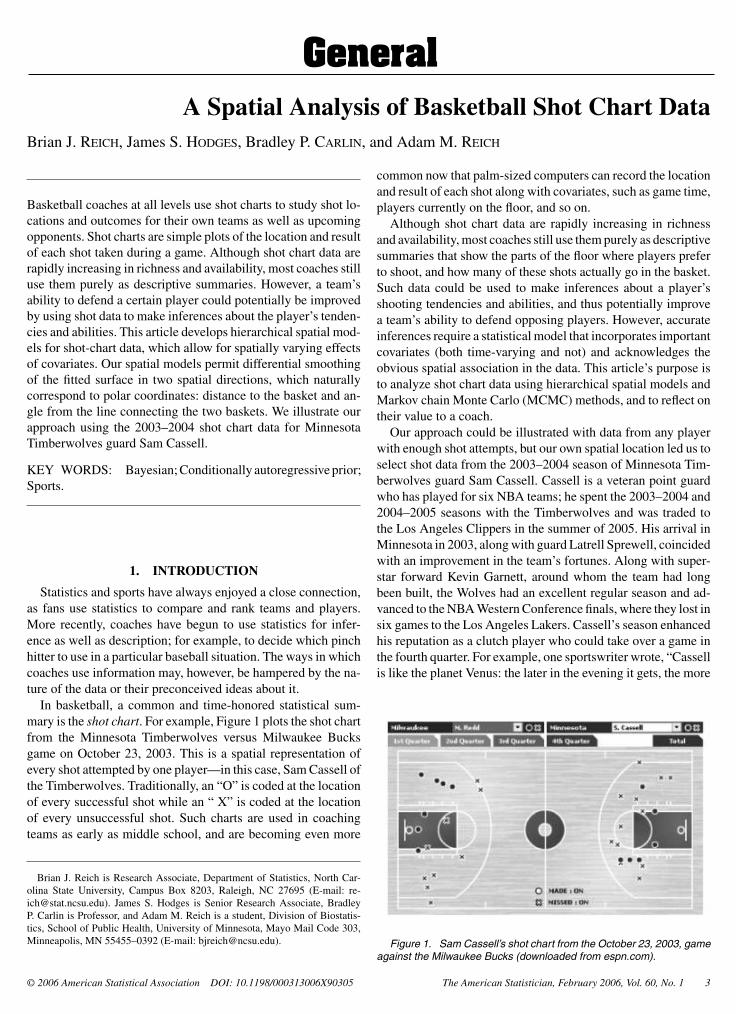
In basketball, a common and time-honored statistical sum-mary is the shot chart. For example, Figure 1 plots the shot chartfrom the Minnesota Timberwolves versus Milwaukee Bucksgame on October 23, 2003. This is a spatial representation ofevery shot attempted by one player—in this case, Sam Cassell ofthe Timberwolves. Traditionally, an “O” is coded at the locationof every successful shot while an “ X” is coded at the locationof every unsuccessful shot. Such charts are used in coachingteams as early as middle school, and are becoming even more

Brian J. Reich is Research Associate, Department of Statistics, North Car-olina State University, Campus Box 8203, Raleigh, NC 27695 (E-mail: re-ich@stat.ncsu.edu). James S. Hodges is Senior Research Associate, BradleyP. Carlin is Professor, and Adam M. Reich is a student, Division of Biostatis-tics, School of Public Health, University of Minnesota, Mayo Mail Code 303,Minneapolis, MN 55455–0392 (E-mail: bjreich@ncsu.edu).

common now that palm-sized computers can record the locationand result of each shot along with covariates, such as game time,players currently on the floor, and so on.

Although shot chart data are rapidly increasing in richnessand availability, most coaches still use them purely as descriptivesummaries that show the parts of the floor where players preferto shoot, and how many of these shots actually go in the basket.Such data could be used to make inferences about a player’sshooting tendencies and abilities, and thus potentially improvea team’s ability to defend opposing players. However, accurateinferences require a statistical model that incorporates importantcovariates (both time-varying and not) and acknowledges theobvious spatial association in the data. This article’s purpose isto analyze shot chart data using hierarchical spatial models andMarkov chain Monte Carlo (MCMC) methods, and to reflect ontheir value to a coach.

Our approach could be illustrated with data from any playerwith enough shot attempts, but our own spatial location led us toselect shot data from the 2003–2004 season of Minnesota Tim-berwolves guard Sam Cassell. Cassell is a veteran point guardwho has played for six NBA teams; he spent the 2003–2004 and2004–2005 seasons with the Timberwolves and was traded tothe Los Angeles Clippers in the summer of 2005. His arrival inMinnesota in 2003, along with guard Latrell Sprewell, coincidedwith an improvement in the team’s fortunes. Along with super-star forward Kevin Garnett, around whom the team had longbeen built, the Wolves had an excellent regular season and ad-vanced to the NBA Western Conference finals, where they lost insix games to the Los Angeles Lakers. Cassell’s season enhancedhis reputation as a clutch player who could take over a game inthe fourth quarter. For example, one sportswriter wrote, “Cassellis like the planet Venus: the later in the evening it gets, the more

Figure 1. Sam Cassell’s shot chart from the October 23, 2003, gameagainst the Milwaukee Bucks (downloaded from espn.com).

© 2006 American Statistical Association DOI: 10.1198/000313006X90305 The American Statistician, February 2006, Vol. 60, No. 1 3

visible he becomes to the naked eye,” (Powers 2004) while an-other opined, “The reason for Cassell being better late in games?A simple combination of having the ball on every possession,and then being absolutely, positively, completely unconcernedwith whether he falls flat on his face” (Hamilton 2004).

Our data, downloaded from espn.com, are 90% complete: ofthe 1,270 shots Cassell took during the 2003–2004 season, wehave full information for N = 1,139. Six games’ data wereunavailable, and a few shots were recorded in game summariesbut not on the shot chart. For each shot, we have game clock timeelapsed since Cassell’s last shot (excluding time on the bench),its location in polar coordinates, that is, feet from the basket andangle from the center line, its result (make or miss), and 10 binarycovariates (Table 1). Some of these covariates are dichotomizedcontinuous covariates, for example, BEHIND is derived from thegame’s current score. Binary covariates improve computationalefficiency immensely at a relatively low cost in lost information;we comment further below.

Table 1 anticipates that the absence of two players, Garnettand Sprewell, may affect Cassell’s shooting. Garnett, Sprewell,and Cassell scored 64% of Minnesota’s points in 2003–2004, ahigher percentage than any other trio in the league. No other Tim-berwolves player scored more than 7% of the team’s points, sono other player’s presence is likely to affect Cassell’s shooting.

Table 1. Description of the Binary Covariates Measured atthe Time of Each Shot Attempt

Name The covariate equals one when: Frequency

NOKG Kevin Garnett is not in

the game

0.13

NOLS Latrell Sprewell is not in

the game

0.21

HOME The game is played in

Minnesota

0.55

NOREST The Timberwolves had

less than 2 days off

since their last game

0.72

2HALF/OT Second half or overtime 0.48

BEHIND The Timberwolves are

losing

0.37

BLOCK The opponent averages

more than 4.8 blocks

per game

0.48

FGPALL The opponent allowed

a field goal percentage

under 44%

0.50

MISSLAST Cassell missed his pre-

vious shot

0.47

TEAMFGA The Timberwolves took

more that 80 shots in the

current game

0.51

Our statistical models also consider the NOKG × NOLS inter-action term because Cassell’s performance may only be affectedby both players’ absence. Team success is known to be affectedby HOME and NOREST, so these covariates are included as pre-dictors of Cassell’s shooting. The current game situation, repre-sented by 2HALF/OT, BEHIND, and 2HALF/OT × BEHIND,could influence offensive strategy and thus Cassell’s shot selec-tion. MISSLAST is used to test conjectures relating to the so-called “hot hand” theory that past results affect current shot se-lection and success (Larkey, Smith, and Kadane 1989; Gilovich,Valone, and Tversky 1985; Tversky and Gilovich 1989; Albright1993). Other predictors of Cassell’s shooting are BLOCK andFGPALL, which represent the opponent’s defensive prowess,and TEAMFGA which measures the game’s tempo.

The rest of the article is as follows. Section 2 considers rel-atively simple models for the time between Cassell’s shots. Al-though time between shots is not recorded in a shot chart, whichis our primary focus, these data help paint a complete picture ofCassell’s shooting tendencies. These models do not have spatialor temporal random effects, but offer a quick, simple look at anaspect of the data that does not seem to justify more intensiveanalysis. Section 3 turns to analyzing factors affecting Cassell’schoice of locations for taking shots. Here spatial correlation isimportant; we use conditionally autoregressive (CAR) modelsthat allow for differential smoothing in the two relevant spatialcoordinates, distance from the basket and angle relative to thecenter line. Section 4 considers shot success, again accountingfor covariates and the similarity of outcomes from shots taken atproximate locations. The last two sections use a recently devel-oped model evaluation tool, the deviance information criterion(DIC; Spiegelhalter, Best, Carlin, and van der Linde 2002) tochoose among competing models. Finally, Section 5 summa-rizes the findings and suggests avenues for future research inthis area.

2. SHOT FREQUENCY

Cassell attempted an average of 15.0 shots per game and themedian game time between his shots, excluding game time whenhe was not in the game, was 1.6 minutes. To assess factors as-sociated with his shot frequency, we used a multiple linear re-gression with the log of the time between shot attempts as theresponse, main effects for each covariate in Table 1, interactioneffects for NOKG×NOLS and BEHIND×2HALF/OT, andhomogeneous error variance. We chose diffuse normal priorswith mean 0, variance 1,000 for the mean parameters and anIG(0.01, 0.01) prior for the error variance, where IG(α1, α2)denotes the inverse gamma distribution with density propor-tional to (σ2

e)−(α1+1) exp (−α2/σ

2e). Although Daniels and

Kass (1999) showed that IG(ε, ε) priors may not be truly “non-informative” in the sense that changing εmay lead to substantivechanges in the posterior for σ2

e , such changes typically do notimpact the mean parameters’ posteriors which are our primaryfocus.

The covariates NOKG, NOLS, and BEHIND can change be-tween shot attempts; because their values are recorded only atthe time of each shot, we do not have the exact times when thesecovariates changed values. One possible remedy is an error-in-covariates model, where the known binary (0/1) covariate Xki

4 General

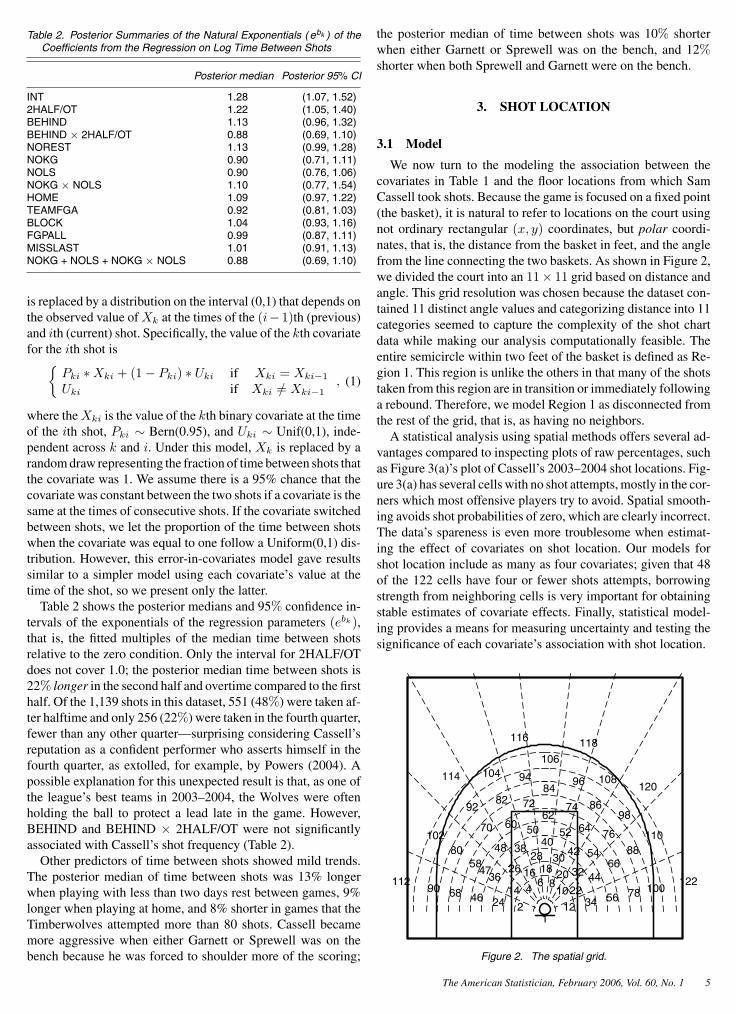
Table 2. Posterior Summaries of the Natural Exponentials ( ebk ) of theCoefficients from the Regression on Log Time Between Shots

Posterior median Posterior 95% CI

INT 1.28 (1.07, 1.52)2HALF/OT 1.22 (1.05, 1.40)BEHIND 1.13 (0.96, 1.32)BEHIND × 2HALF/OT 0.88 (0.69, 1.10)NOREST 1.13 (0.99, 1.28)NOKG 0.90 (0.71, 1.11)NOLS 0.90 (0.76, 1.06)NOKG × NOLS 1.10 (0.77, 1.54)HOME 1.09 (0.97, 1.22)TEAMFGA 0.92 (0.81, 1.03)BLOCK 1.04 (0.93, 1.16)FGPALL 0.99 (0.87, 1.11)MISSLAST 1.01 (0.91, 1.13)NOKG + NOLS + NOKG × NOLS 0.88 (0.69, 1.10)

is replaced by a distribution on the interval (0,1) that depends onthe observed value of Xk at the times of the (i− 1)th (previous)and ith (current) shot. Specifically, the value of the kth covariatefor the ith shot is{

Pki ∗ Xki + (1 − Pki) ∗ Uki if Xki = Xki−1Uki if Xki /= Xki−1

, (1)

where the Xki is the value of the kth binary covariate at the timeof the ith shot, Pki ∼ Bern(0.95), and Uki ∼ Unif(0,1), inde-pendent across k and i. Under this model, Xk is replaced by arandom draw representing the fraction of time between shots thatthe covariate was 1. We assume there is a 95% chance that thecovariate was constant between the two shots if a covariate is thesame at the times of consecutive shots. If the covariate switchedbetween shots, we let the proportion of the time between shotswhen the covariate was equal to one follow a Uniform(0,1) dis-tribution. However, this error-in-covariates model gave resultssimilar to a simpler model using each covariate’s value at thetime of the shot, so we present only the latter.

Table 2 shows the posterior medians and 95% confidence in-tervals of the exponentials of the regression parameters (ebk),that is, the fitted multiples of the median time between shotsrelative to the zero condition. Only the interval for 2HALF/OTdoes not cover 1.0; the posterior median time between shots is22% longer in the second half and overtime compared to the firsthalf. Of the 1,139 shots in this dataset, 551 (48%) were taken af-ter halftime and only 256 (22%) were taken in the fourth quarter,fewer than any other quarter—surprising considering Cassell’sreputation as a confident performer who asserts himself in thefourth quarter, as extolled, for example, by Powers (2004). Apossible explanation for this unexpected result is that, as one ofthe league’s best teams in 2003–2004, the Wolves were oftenholding the ball to protect a lead late in the game. However,BEHIND and BEHIND × 2HALF/OT were not significantlyassociated with Cassell’s shot frequency (Table 2).

Other predictors of time between shots showed mild trends.The posterior median of time between shots was 13% longerwhen playing with less than two days rest between games, 9%longer when playing at home, and 8% shorter in games that theTimberwolves attempted more than 80 shots. Cassell becamemore aggressive when either Garnett or Sprewell was on thebench because he was forced to shoulder more of the scoring;

the posterior median of time between shots was 10% shorterwhen either Garnett or Sprewell was on the bench, and 12%shorter when both Sprewell and Garnett were on the bench.

3. SHOT LOCATION

3.1 Model

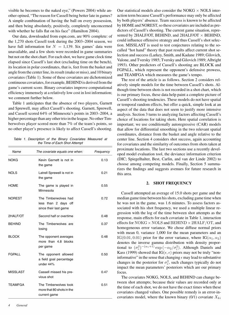
We now turn to the modeling the association between thecovariates in Table 1 and the floor locations from which SamCassell took shots. Because the game is focused on a fixed point(the basket), it is natural to refer to locations on the court usingnot ordinary rectangular (x, y) coordinates, but polar coordi-nates, that is, the distance from the basket in feet, and the anglefrom the line connecting the two baskets. As shown in Figure 2,we divided the court into an 11× 11 grid based on distance andangle. This grid resolution was chosen because the dataset con-tained 11 distinct angle values and categorizing distance into 11categories seemed to capture the complexity of the shot chartdata while making our analysis computationally feasible. Theentire semicircle within two feet of the basket is defined as Re-gion 1. This region is unlike the others in that many of the shotstaken from this region are in transition or immediately followinga rebound. Therefore, we model Region 1 as disconnected fromthe rest of the grid, that is, as having no neighbors.

A statistical analysis using spatial methods offers several ad-vantages compared to inspecting plots of raw percentages, suchas Figure 3(a)’s plot of Cassell’s 2003–2004 shot locations. Fig-ure 3(a) has several cells with no shot attempts, mostly in the cor-ners which most offensive players try to avoid. Spatial smooth-ing avoids shot probabilities of zero, which are clearly incorrect.The data’s spareness is even more troublesome when estimat-ing the effect of covariates on shot location. Our models forshot location include as many as four covariates; given that 48of the 122 cells have four or fewer shots attempts, borrowingstrength from neighboring cells is very important for obtainingstable estimates of covariate effects. Finally, statistical model-ing provides a means for measuring uncertainty and testing thesignificance of each covariate’s association with shot location.

Figure 2. The spatial grid.

The American Statistician, February 2006, Vol. 60, No. 1 5

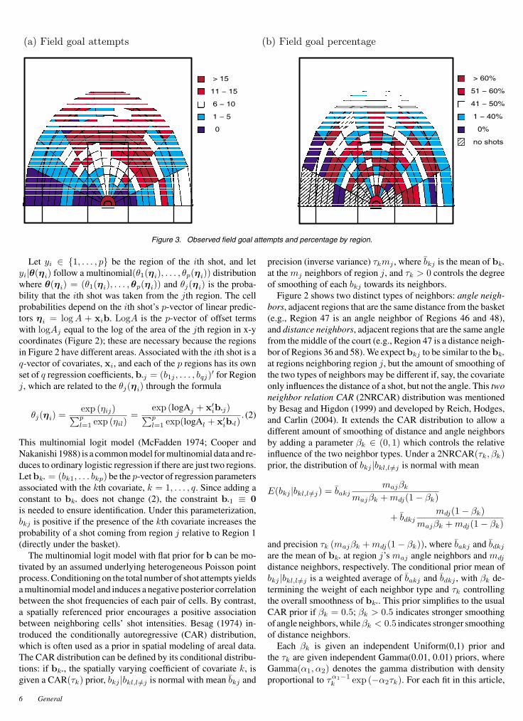
Figure 3. Observed field goal attempts and percentage by region.

Let yi ∈ {1, . . . , p} be the region of the ith shot, and letyi|θ(ηi) follow a multinomial(θ1(ηi), . . . , θp(ηi)) distributionwhere θ(ηi) = (θ1(ηi), . . . ,θp(ηi)) and θj(ηi) is the proba-bility that the ith shot was taken from the jth region. The cellprobabilities depend on the ith shot’s p-vector of linear predic-tors ηi = logA + xib. LogA is the p-vector of offset termswith logAj equal to the log of the area of the jth region in x-ycoordinates (Figure 2); these are necessary because the regionsin Figure 2 have different areas. Associated with the ith shot is aq-vector of covariates, xi, and each of the p regions has its ownset of q regression coefficients, b j = (b1j , . . . , bqj)′ for Regionj, which are related to the θj(ηi) through the formula

θj(ηi) =exp (ηij)∑pl=1 exp (ηil)

=exp (logAj + x′

ib j)∑pl=1 exp(logAl + x′

ib l). (2)

This multinomial logit model (McFadden 1974; Cooper andNakanishi 1988) is a common model for multinomial data and re-duces to ordinary logistic regression if there are just two regions.Let bk = (bk1, . . . bkp) be the p-vector of regression parametersassociated with the kth covariate, k = 1, . . . , q. Since adding aconstant to bk does not change (2), the constraint b 1 ≡ 0is needed to ensure identification. Under this parameterization,bkj is positive if the presence of the kth covariate increases theprobability of a shot coming from region j relative to Region 1(directly under the basket).

The multinomial logit model with flat prior for b can be mo-tivated by an assumed underlying heterogeneous Poisson pointprocess. Conditioning on the total number of shot attempts yieldsa multinomial model and induces a negative posterior correlationbetween the shot frequencies of each pair of cells. By contrast,a spatially referenced prior encourages a positive associationbetween neighboring cells’ shot intensities. Besag (1974) in-troduced the conditionally autoregressive (CAR) distribution,which is often used as a prior in spatial modeling of areal data.The CAR distribution can be defined by its conditional distribu-tions: if bk , the spatially varying coefficient of covariate k, isgiven a CAR(τk) prior, bkj |bkl,l /=j is normal with mean b̄kj and

precision (inverse variance) τkmj , where b̄kj is the mean of bk

at the mj neighbors of region j, and τk > 0 controls the degreeof smoothing of each bkj towards its neighbors.

Figure 2 shows two distinct types of neighbors: angle neigh-bors, adjacent regions that are the same distance from the basket(e.g., Region 47 is an angle neighbor of Regions 46 and 48),and distance neighbors, adjacent regions that are the same anglefrom the middle of the court (e.g., Region 47 is a distance neigh-bor of Regions 36 and 58). We expect bkj to be similar to the bk

at regions neighboring region j, but the amount of smoothing ofthe two types of neighbors may be different if, say, the covariateonly influences the distance of a shot, but not the angle. This twoneighbor relation CAR (2NRCAR) distribution was mentionedby Besag and Higdon (1999) and developed by Reich, Hodges,and Carlin (2004). It extends the CAR distribution to allow adifferent amount of smoothing of distance and angle neighborsby adding a parameter βk ∈ (0, 1) which controls the relativeinfluence of the two neighbor types. Under a 2NRCAR(τk, βk)prior, the distribution of bkj |bkl,l /=j is normal with mean

E(bkj |bkl,l /=j) = b̄akjmajβk

majβk +mdj(1 − βk)

+ b̄dkjmdj(1 − βk)

majβk +mdj(1 − βk)

and precision τk (majβk +mdj(1 − βk)), where b̄akj and b̄dkj

are the mean of bk at region j’s maj angle neighbors and mdj

distance neighbors, respectively. The conditional prior mean ofbkj |bkl,l /=j is a weighted average of b̄akj and b̄dkj , with βk de-termining the weight of each neighbor type and τk controllingthe overall smoothness of bk . This prior simplifies to the usualCAR prior if βk = 0.5; βk > 0.5 indicates stronger smoothingof angle neighbors, whileβk < 0.5 indicates stronger smoothingof distance neighbors.

Each βk is given an independent Uniform(0,1) prior andthe τk are given independent Gamma(0.01, 0.01) priors, whereGamma(α1, α2) denotes the gamma distribution with densityproportional to τα1−1

k exp (−α2τk). For each fit in this article,

6 General

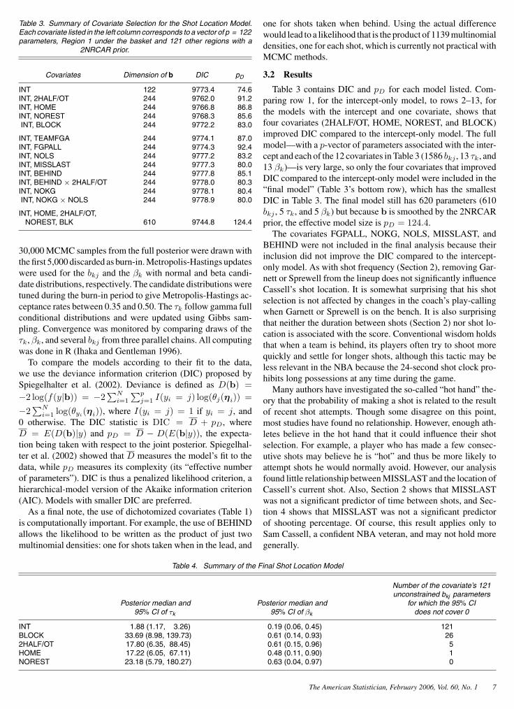
Table 3. Summary of Covariate Selection for the Shot Location Model.Each covariate listed in the left column corresponds to a vector of p = 122parameters, Region 1 under the basket and 121 other regions with a

2NRCAR prior.

Covariates Dimension of b DIC pD

INT 122 9773.4 74.6INT, 2HALF/OT 244 9762.0 91.2INT, HOME 244 9766.8 86.8INT, NOREST 244 9768.3 85.6INT, BLOCK 244 9772.2 83.0

INT, TEAMFGA 244 9774.1 87.0INT, FGPALL 244 9774.3 92.4INT, NOLS 244 9777.2 83.2INT, MISSLAST 244 9777.3 80.0INT, BEHIND 244 9777.8 85.1INT, BEHIND × 2HALF/OT 244 9778.0 80.3INT, NOKG 244 9778.1 80.4INT, NOKG × NOLS 244 9778.9 80.0

INT, HOME, 2HALF/OT,NOREST, BLK 610 9744.8 124.4

30,000 MCMC samples from the full posterior were drawn withthe first 5,000 discarded as burn-in. Metropolis-Hastings updateswere used for the bkj and the βk with normal and beta candi-date distributions, respectively. The candidate distributions weretuned during the burn-in period to give Metropolis-Hastings ac-ceptance rates between 0.35 and 0.50. The τk follow gamma fullconditional distributions and were updated using Gibbs sam-pling. Convergence was monitored by comparing draws of theτk, βk, and several bkj from three parallel chains. All computingwas done in R (Ihaka and Gentleman 1996).

To compare the models according to their fit to the data,we use the deviance information criterion (DIC) proposed bySpiegelhalter et al. (2002). Deviance is defined as D(b) =−2 log(f(y|b)) = −2

∑Ni=1

∑pj=1 I(yi = j) log(θj(ηi)) =

−2∑N

i=1 log(θyi(ηi)), where I(yi = j) = 1 if yi = j, and

0 otherwise. The DIC statistic is DIC = D + pD, whereD = E(D(b)|y) and pD = D − D(E(b|y)), the expecta-tion being taken with respect to the joint posterior. Spiegelhal-ter et al. (2002) showed that D measures the model’s fit to thedata, while pD measures its complexity (its “effective numberof parameters”). DIC is thus a penalized likelihood criterion, ahierarchical-model version of the Akaike information criterion(AIC). Models with smaller DIC are preferred.

As a final note, the use of dichotomized covariates (Table 1)is computationally important. For example, the use of BEHINDallows the likelihood to be written as the product of just twomultinomial densities: one for shots taken when in the lead, and

one for shots taken when behind. Using the actual differencewould lead to a likelihood that is the product of 1139 multinomialdensities, one for each shot, which is currently not practical withMCMC methods.

3.2 Results

Table 3 contains DIC and pD for each model listed. Com-paring row 1, for the intercept-only model, to rows 2–13, forthe models with the intercept and one covariate, shows thatfour covariates (2HALF/OT, HOME, NOREST, and BLOCK)improved DIC compared to the intercept-only model. The fullmodel—with a p-vector of parameters associated with the inter-cept and each of the 12 covariates in Table 3 (1586 bkj , 13 τk, and13 βk)—is very large, so only the four covariates that improvedDIC compared to the intercept-only model were included in the“final model” (Table 3’s bottom row), which has the smallestDIC in Table 3. The final model still has 620 parameters (610bkj , 5 τk, and 5 βk) but because b is smoothed by the 2NRCARprior, the effective model size is pD = 124.4.

The covariates FGPALL, NOKG, NOLS, MISSLAST, andBEHIND were not included in the final analysis because theirinclusion did not improve the DIC compared to the intercept-only model. As with shot frequency (Section 2), removing Gar-nett or Sprewell from the lineup does not significantly influenceCassell’s shot location. It is somewhat surprising that his shotselection is not affected by changes in the coach’s play-callingwhen Garnett or Sprewell is on the bench. It is also surprisingthat neither the duration between shots (Section 2) nor shot lo-cation is associated with the score. Conventional wisdom holdsthat when a team is behind, its players often try to shoot morequickly and settle for longer shots, although this tactic may beless relevant in the NBA because the 24-second shot clock pro-hibits long possessions at any time during the game.

Many authors have investigated the so-called “hot hand” the-ory that the probability of making a shot is related to the resultof recent shot attempts. Though some disagree on this point,most studies have found no relationship. However, enough ath-letes believe in the hot hand that it could influence their shotselection. For example, a player who has made a few consec-utive shots may believe he is “hot” and thus be more likely toattempt shots he would normally avoid. However, our analysisfound little relationship between MISSLAST and the location ofCassell’s current shot. Also, Section 2 shows that MISSLASTwas not a significant predictor of time between shots, and Sec-tion 4 shows that MISSLAST was not a significant predictorof shooting percentage. Of course, this result applies only toSam Cassell, a confident NBA veteran, and may not hold moregenerally.

Table 4. Summary of the Final Shot Location Model

Number of the covariate’s 121unconstrained bkj parameters

Posterior median and Posterior median and for which the 95% CI95% CI of τk 95% CI of βk does not cover 0

INT 1.88 (1.17, 3.26) 0.19 (0.06, 0.45) 121BLOCK 33.69 (8.98, 139.73) 0.61 (0.14, 0.93) 262HALF/OT 17.80 (6.35, 88.45) 0.61 (0.15, 0.96) 5HOME 17.22 (6.05, 67.11) 0.48 (0.11, 0.90) 1NOREST 23.18 (5.79, 180.27) 0.63 (0.04, 0.97) 0

The American Statistician, February 2006, Vol. 60, No. 1 7

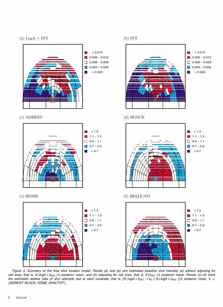
Figure 4. Summary of the final shot location model. Panels (a) and (b) plot estimated baseline shot intensity (a) without adjusting forcell area, that is, θ ( logA + bINT ·)’s posterior mean, and (b) adjusting for cell area, that is, θ ( bINT ·)’s posterior mean. Panels (c)–(f) showthe estimated relative risks of shot attempts due to each covariate, that is, [ θ ( logA + bINT · + bk ·) /θ ( logA + bINT ·)] ’s posterior mean, k ∈{NOREST, BLOCK, HOME, 2HALF/OT}.

8 General

The final model has slightly smaller DIC (9744.8) than themodel with the same covariates but with βk = 0.5, k = 1, . . . , q(DIC = 9749.1). Table 4 summarizes the posteriors of thesmoothing parameters {τk, βk} in the final model. The posteriormedian of the smoothing precision τk is smallest for the inter-cept, indicating more spatial variation in the intercept than in anyof the coefficients. For the intercept, βk has posterior median0.19 and its 95% confidence interval does not cover 0.5, that is,distance neighbors appear to be significantly more similar thanangle neighbors. For BLOCK, 2HALF/OT, and NOREST, theposterior median of βk is greater than 0.5 (stronger smoothing ofangle neighbors), suggesting these covariates have more influ-ence on the distance of the shot than the angle. However, the dataprovide little information about βk, whose posterior confidenceintervals cover 0.50 and indeed most of the unit interval.

Figure 4 illustrates the effect of each covariate’s effect onshot location. As the intercept’s small τk indicated, there is lit-tle smoothing of the intercept parameters. The plot of θ(logA+bINT·)’s posterior mean (Figure 4(a)), that is, the estimated base-line shot intensity, resembles the plot of the observed numberof shot attempts (Figure 3(a)). Figure 4(b) plots the estimatedbaseline shot intensities adjusted for the different area of the gridsquares; predictably, this shifts mass toward the basket where thegrid squares are smaller. For each region other than Region 1, theposterior 95% confidence interval of the bINTj does not coverzero and the posterior mean is negative. That is, Cassell’s favoriteregion is right at the basket. His next favorite type of shot is themid-range shot from 12–20 feet. From all distances, he prefersshots from the center of the court and has a preference for shoot-ing from left of the center line. Cassell’s preference for shootingfrom the left side of the court does not necessarily indicate heprefers dribbling with his left hand; investigating dribbling ten-dencies requires data that are not included in shot charts, forexample, the number of dribbles taken with each hand.

Although NOREST was included in the final model, the 95%confidence intervals for its bjk cover zero at all 122 regions(Table 4). When playing on less than two days rest, Cassell

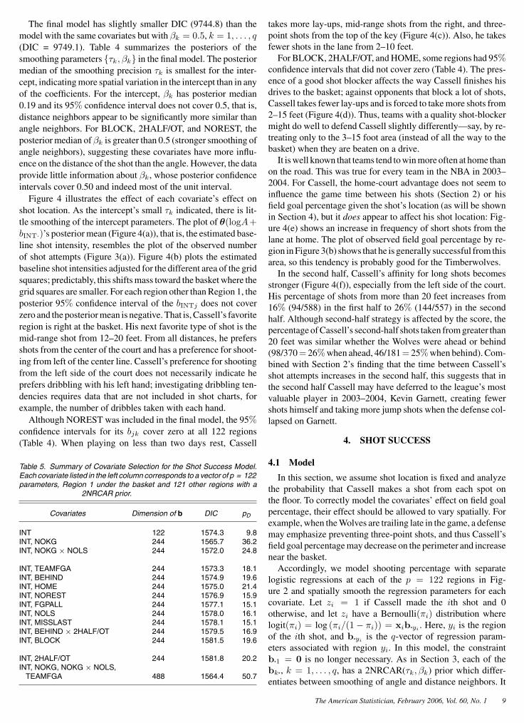
Table 5. Summary of Covariate Selection for the Shot Success Model.Each covariate listed in the left column corresponds to a vector of p = 122parameters, Region 1 under the basket and 121 other regions with a

2NRCAR prior.

Covariates Dimension of b DIC pD

INT 122 1574.3 9.8INT, NOKG 244 1565.7 36.2INT, NOKG × NOLS 244 1572.0 24.8

INT, TEAMFGA 244 1573.3 18.1INT, BEHIND 244 1574.9 19.6INT, HOME 244 1575.0 21.4INT, NOREST 244 1576.9 15.9INT, FGPALL 244 1577.1 15.1INT, NOLS 244 1578.0 16.1INT, MISSLAST 244 1578.1 15.1INT, BEHIND × 2HALF/OT 244 1579.5 16.9INT, BLOCK 244 1581.5 19.6

INT, 2HALF/OT 244 1581.8 20.2INT, NOKG, NOKG × NOLS,

TEAMFGA 488 1564.4 50.7

takes more lay-ups, mid-range shots from the right, and three-point shots from the top of the key (Figure 4(c)). Also, he takesfewer shots in the lane from 2–10 feet.

For BLOCK, 2HALF/OT, and HOME, some regions had 95%confidence intervals that did not cover zero (Table 4). The pres-ence of a good shot blocker affects the way Cassell finishes hisdrives to the basket; against opponents that block a lot of shots,Cassell takes fewer lay-ups and is forced to take more shots from2–15 feet (Figure 4(d)). Thus, teams with a quality shot-blockermight do well to defend Cassell slightly differently—say, by re-treating only to the 3–15 foot area (instead of all the way to thebasket) when they are beaten on a drive.

It is well known that teams tend to win more often at home thanon the road. This was true for every team in the NBA in 2003–2004. For Cassell, the home-court advantage does not seem toinfluence the game time between his shots (Section 2) or hisfield goal percentage given the shot’s location (as will be shownin Section 4), but it does appear to affect his shot location: Fig-ure 4(e) shows an increase in frequency of short shots from thelane at home. The plot of observed field goal percentage by re-gion in Figure 3(b) shows that he is generally successful from thisarea, so this tendency is probably good for the Timberwolves.

In the second half, Cassell’s affinity for long shots becomesstronger (Figure 4(f)), especially from the left side of the court.His percentage of shots from more than 20 feet increases from16% (94/588) in the first half to 26% (144/557) in the secondhalf. Although second-half strategy is affected by the score, thepercentage of Cassell’s second-half shots taken from greater than20 feet was similar whether the Wolves were ahead or behind(98/370= 26%when ahead, 46/181= 25%when behind). Com-bined with Section 2’s finding that the time between Cassell’sshot attempts increases in the second half, this suggests that inthe second half Cassell may have deferred to the league’s mostvaluable player in 2003–2004, Kevin Garnett, creating fewershots himself and taking more jump shots when the defense col-lapsed on Garnett.

4. SHOT SUCCESS

4.1 Model

In this section, we assume shot location is fixed and analyzethe probability that Cassell makes a shot from each spot onthe floor. To correctly model the covariates’ effect on field goalpercentage, their effect should be allowed to vary spatially. Forexample, when the Wolves are trailing late in the game, a defensemay emphasize preventing three-point shots, and thus Cassell’sfield goal percentage may decrease on the perimeter and increasenear the basket.

Accordingly, we model shooting percentage with separatelogistic regressions at each of the p = 122 regions in Fig-ure 2 and spatially smooth the regression parameters for eachcovariate. Let zi = 1 if Cassell made the ith shot and 0otherwise, and let zi have a Bernoulli(πi) distribution wherelogit(πi) = log (πi/(1 − πi)) = xib yi . Here, yi is the regionof the ith shot, and b yi is the q-vector of regression param-eters associated with region yi. In this model, the constraintb 1 = 0 is no longer necessary. As in Section 3, each of thebk , k = 1, . . . , q, has a 2NRCAR(τk, βk) prior which differ-entiates between smoothing of angle and distance neighbors. It

The American Statistician, February 2006, Vol. 60, No. 1 9

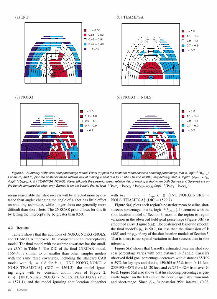
Figure 5. Summary of the final shot percentage model. Panel (a) plots the posterior mean baseline shooting percentage, that is, logit −1( bINT j ).Panels (b) and (c) plot the posterior mean relative risk of making a shot due to TEAMFGA and NOKG, respectively, that is, logit −1( bINT j + bkj )/logit−1( bINT j ), k ∈ {TEAMFGA; NOKG}. Panel (d) plots the posterior mean relative risk of making a shot when both Garnett and Sprewell are onthe bench compared to when only Garnett is on the bench, that is, logit−1( bINT j + bNOKGj + bNOKG×NOLSj )/logit −1( bINT j + bNOKGj ).

seems reasonable that shot success will be affected more by dis-tance than angle: changing the angle of a shot has little effecton shooting technique, while longer shots are generally moredifficult than short shots. The 2NRCAR prior allows for this fitby letting the intercept’s βk be greater than 0.50.

4.2 Results

Table 5 shows that the additions of NOKG, NOKG×NOLS,and TEAMFGA improved DIC compared to the intercept-onlymodel. The final model with these three covariates has the small-est DIC in Table 5. The DIC of the final 2NRCAR model,1564.4, is similar to or smaller than other, simpler modelswith the same three covariates, including the standard CARmodel with βk = 0.5 for k ∈ {INT,NOKG,NOKG ×NOLS,TEAMFGA} (DIC = 1564.2), the model ignor-ing angle with bk constant within rows of Figure 2,k ∈ {INT,NOKG,NOKG × NOLS,TEAMFGA} (DIC= 1571.1), and the model ignoring shot location altogether

with bk1 = · · · = bkp, k ∈ {INT,NOKG,NOKG ×NOLS,TEAMFGA} (DIC = 1579.7).

Figure 5(a) plots each region’s posterior mean baseline shot-success percentage, that is, logit−1(bINTj). In contrast with theshot location model of Section 3, most of the region-to-regionvariation in the observed field goal percentage (Figure 3(b)) issmoothed away (Figure 5(a)). The posterior of b is quite smooth;the final model’s pD is 50.7, far less than the dimension of b(488) and the pD of any of the shot location models of Section 3.That is, there is less spatial variation in shot success than in shotintensity.

Figure 5(a) shows that Cassell’s estimated baseline shot suc-cess percentage varies with both distance and angle. Cassell’sobserved field goal percentage decreases with distance (65/109= 59% for lay-ups and dunks, 159/305 = 52% from 0–14 feet,233/490 = 48% from 15–20 feet, and 99/237 = 42% from over 20feet). Figure 5(a) also shows that his shooting percentage is gen-erally higher on the left side of the court, especially from mid-and short-range. Since βINT’s posterior 95% interval, (0.08,

10 General

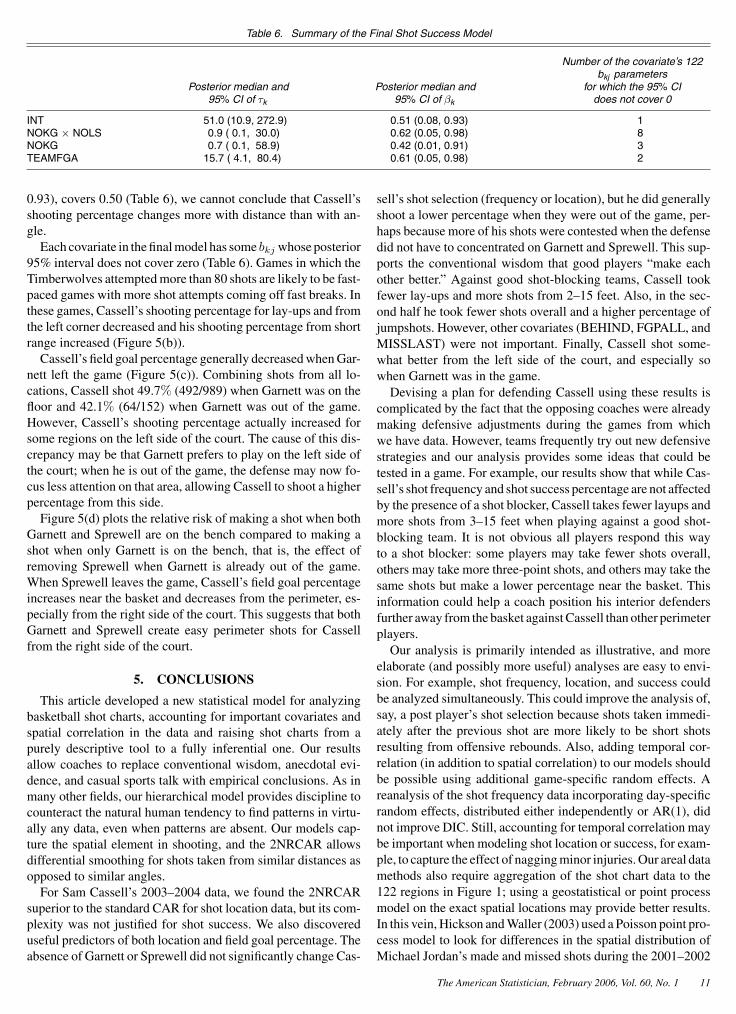
Table 6. Summary of the Final Shot Success Model

Number of the covariate’s 122bkj parameters

Posterior median and Posterior median and for which the 95% CI95% CI of τk 95% CI of βk does not cover 0

INT 51.0 (10.9, 272.9) 0.51 (0.08, 0.93) 1NOKG × NOLS 0.9 ( 0.1, 30.0) 0.62 (0.05, 0.98) 8NOKG 0.7 ( 0.1, 58.9) 0.42 (0.01, 0.91) 3TEAMFGA 15.7 ( 4.1, 80.4) 0.61 (0.05, 0.98) 2

0.93), covers 0.50 (Table 6), we cannot conclude that Cassell’sshooting percentage changes more with distance than with an-gle.

Each covariate in the final model has some bkj whose posterior95% interval does not cover zero (Table 6). Games in which theTimberwolves attempted more than 80 shots are likely to be fast-paced games with more shot attempts coming off fast breaks. Inthese games, Cassell’s shooting percentage for lay-ups and fromthe left corner decreased and his shooting percentage from shortrange increased (Figure 5(b)).

Cassell’s field goal percentage generally decreased when Gar-nett left the game (Figure 5(c)). Combining shots from all lo-cations, Cassell shot 49.7% (492/989) when Garnett was on thefloor and 42.1% (64/152) when Garnett was out of the game.However, Cassell’s shooting percentage actually increased forsome regions on the left side of the court. The cause of this dis-crepancy may be that Garnett prefers to play on the left side ofthe court; when he is out of the game, the defense may now fo-cus less attention on that area, allowing Cassell to shoot a higherpercentage from this side.

Figure 5(d) plots the relative risk of making a shot when bothGarnett and Sprewell are on the bench compared to making ashot when only Garnett is on the bench, that is, the effect ofremoving Sprewell when Garnett is already out of the game.When Sprewell leaves the game, Cassell’s field goal percentageincreases near the basket and decreases from the perimeter, es-pecially from the right side of the court. This suggests that bothGarnett and Sprewell create easy perimeter shots for Cassellfrom the right side of the court.

5. CONCLUSIONS

This article developed a new statistical model for analyzingbasketball shot charts, accounting for important covariates andspatial correlation in the data and raising shot charts from apurely descriptive tool to a fully inferential one. Our resultsallow coaches to replace conventional wisdom, anecdotal evi-dence, and casual sports talk with empirical conclusions. As inmany other fields, our hierarchical model provides discipline tocounteract the natural human tendency to find patterns in virtu-ally any data, even when patterns are absent. Our models cap-ture the spatial element in shooting, and the 2NRCAR allowsdifferential smoothing for shots taken from similar distances asopposed to similar angles.

For Sam Cassell’s 2003–2004 data, we found the 2NRCARsuperior to the standard CAR for shot location data, but its com-plexity was not justified for shot success. We also discovereduseful predictors of both location and field goal percentage. Theabsence of Garnett or Sprewell did not significantly change Cas-

sell’s shot selection (frequency or location), but he did generallyshoot a lower percentage when they were out of the game, per-haps because more of his shots were contested when the defensedid not have to concentrated on Garnett and Sprewell. This sup-ports the conventional wisdom that good players “make eachother better.” Against good shot-blocking teams, Cassell tookfewer lay-ups and more shots from 2–15 feet. Also, in the sec-ond half he took fewer shots overall and a higher percentage ofjumpshots. However, other covariates (BEHIND, FGPALL, andMISSLAST) were not important. Finally, Cassell shot some-what better from the left side of the court, and especially sowhen Garnett was in the game.

Devising a plan for defending Cassell using these results iscomplicated by the fact that the opposing coaches were alreadymaking defensive adjustments during the games from whichwe have data. However, teams frequently try out new defensivestrategies and our analysis provides some ideas that could betested in a game. For example, our results show that while Cas-sell’s shot frequency and shot success percentage are not affectedby the presence of a shot blocker, Cassell takes fewer layups andmore shots from 3–15 feet when playing against a good shot-blocking team. It is not obvious all players respond this wayto a shot blocker: some players may take fewer shots overall,others may take more three-point shots, and others may take thesame shots but make a lower percentage near the basket. Thisinformation could help a coach position his interior defendersfurther away from the basket against Cassell than other perimeterplayers.

Our analysis is primarily intended as illustrative, and moreelaborate (and possibly more useful) analyses are easy to envi-sion. For example, shot frequency, location, and success couldbe analyzed simultaneously. This could improve the analysis of,say, a post player’s shot selection because shots taken immedi-ately after the previous shot are more likely to be short shotsresulting from offensive rebounds. Also, adding temporal cor-relation (in addition to spatial correlation) to our models shouldbe possible using additional game-specific random effects. Areanalysis of the shot frequency data incorporating day-specificrandom effects, distributed either independently or AR(1), didnot improve DIC. Still, accounting for temporal correlation maybe important when modeling shot location or success, for exam-ple, to capture the effect of nagging minor injuries. Our areal datamethods also require aggregation of the shot chart data to the122 regions in Figure 1; using a geostatistical or point processmodel on the exact spatial locations may provide better results.In this vein, Hickson and Waller (2003) used a Poisson point pro-cess model to look for differences in the spatial distribution ofMichael Jordan’s made and missed shots during the 2001–2002

The American Statistician, February 2006, Vol. 60, No. 1 11

season. Finally, a coach facing the Timberwolves would need toknow how to defend not only Sam Cassell, but also Garnett andSprewell at the same time. This suggests a multivariate versionof our analysis, perhaps using a multivariate conditionally au-toregressive (MCAR) approach (Gelfand and Vounatsou 2003;Jin, Carlin, and Banerjee in press). Standard (1NR) versions ofthis model are available in the WinBUGS language (http://www.mrc-bsu.cam.ac.uk/bugs/welcome.shtml), while 2NR versionsawait development.

[Received February 2005. Revised October 2005.]

REFERENCES

Albright, S.C. (1993), “A Statistical Analysis of Hitting Streaks in Baseball,”Journal of the American Statistical Association, 88, 1175–1183.

Besag, J. (1974), “Spatial Interaction and the Statistical Analysis of LatticeSystems” (with discussion), Journal of the Royal Statistical Society, SeriesB, 36, 192–236.

Besag, J., and Higdon, D. (1999), “Bayesian Analysis of Agricultural Field Ex-periments” (with discussion), Journal of the Royal Statistical Society, SeriesB, 61, 691–746.

Cooper, L. G., and Nakanishi, M. (1988), Market-Share Analysis: EvaluatingCompetitive Marketing Effectiveness, Boston: Kluwer.

Daniels, M. J., and Kass, R. E. (1999), “Nonconjugate Bayesian Estimationof Covariance Matrices and its use in Hierarchical Models,” Journal of theAmerican Statistical Association, 94, 1254–1263.

Gelfand, A. E., and Vounatsou, P. (2003), “Proper Multivariate Conditional Au-toregressive Models for Spatial Data Analysis,” Biostatistics, 4, 11–25.

Gilovich, T., Vallone, R., and Tversky, A. (1985), “The Hot Hand in Basketball:On the Misperception of Random Sequences,” Cognitive Psychology, 17,295–314.

Hamilton, B. (2004), “Just Call Cassell Mr. Clutch,” Saint Paul Pioneer Press,May 9, 2004.

Hickson, D. A., and Waller, L. A. (2003), “Spatial Analyses of Basketball ShotCharts: An Application to Michael Jordan’s 2001–2002 NBA Season,” Tech-nical Report, Department of Biostatistics, Emory University.

Ihaka, R., and Gentleman, R. (1996), “R: A Language for Data Analysis andGraphics,” Journal of Computational and Graphical Statistics, 5, 299–314.

Jin, X., Carlin, B. P., and Banerjee, S. (in press), “Generalized HierarchicalMultivariate CAR Models for Areal Data,” Biometrics.

Larkey, P. D., Smith, R. A., and Kadane, J. B. (1989), “It’s Okay to Believe inthe ‘Hot Hand,’ ” Chance, 2, 22–30.

McFadden, D. (1974), Conditional Logit Analysis of Qualitative Choice Be-havior. Frontiers of Econometrics, ed. P. Zarembka, New York: AcademicPress.

Powers, T. (2004), “Geezers Gamble Pays Off Big Time,” Saint Paul PioneerPress, Feb 4, 2004.

Reich, B. J., Hodges, J. S., and Carlin, B. P. (2004), “Spatial Analysis of Peri-odontal Data using Conditionally Autoregressive Priors Having Two Types ofNeighbor Relations,” Research Report 2004–2004, Division of Biostatistics,University of Minnesota.

Spiegelhalter, D. J., Best, N. G., Carlin, B. P., and van der Linde, A. (2002),“Bayesian Measures of Model Complexity and Fit” (with discussion), Journalof the Royal Statistical Society, Series B, 64, 583–639.

Tversky, A., and Gilovich, T. (1989), “The ‘Hot Hand’: Statistical Reality orCognitive Illusion?” Chance, 2, 31–34.

12 General