a spatial model of roll call voting: senators ... spatial model of roll call voting: senators,...

A Spatial Model of Roll Call Voting: Senators, Constituents, Presidents, and InterestGroups in Supreme Court ConfirmationsAuthor(s): Jeffrey A. Segal, Charles M. Cameron and Albert D. CoverSource: American Journal of Political Science, Vol. 36, No. 1 (Feb., 1992), pp. 96-121Published by: Midwest Political Science AssociationStable URL: http://www.jstor.org/stable/2111426Accessed: 17-10-2017 16:09 UTC

JSTOR is a not-for-profit service that helps scholars, researchers, and students discover, use, and build upon a wide

range of content in a trusted digital archive. We use information technology and tools to increase productivity and

facilitate new forms of scholarship. For more information about JSTOR, please contact [email protected].

Your use of the JSTOR archive indicates your acceptance of the Terms & Conditions of Use, available at

http://about.jstor.org/terms

Midwest Political Science Association is collaborating with JSTOR to digitize, preserve andextend access to American Journal of Political Science

This content downloaded from 128.112.40.248 on Tue, 17 Oct 2017 16:09:59 UTCAll use subject to http://about.jstor.org/terms

A Spatial Model of Roll Call Voting: Senators, Constituents, Presidents, and Interest Groups in

Supreme Court Confirmations*

Jeffrey A. Segal, State University of New York at Stony Brook

Charles M. Cameron, Columbia University

Albert D. Cover, State University of New York at Stony Brook

We test a spatial model of Supreme Court confirmation votes that examines the effects of

(1) the ideological distance between senators' constituents and nominees, (2) the personal ideologies

of senators, (3) the qualifications of the nominee, (4) the strength of the president, and (5) the

mobilization for and against nominees by interest groups. The data consist of the 1,475 individual

confirmation votes from the 1955 nomination of John Harlan until the 1987-88 nomination of

Anthony Kennedy (voice votes excluded). All of the above factors significantly affect confirmation

voting. The model explains 78% of the variance in senators' decisions, predicts 92% of the individual

votes correctly, and predicts all of the aggregate outcomes correctly.

Introduction

This paper examines a spatial model of roll call voting on Supreme Court nominations from John Harlan (1955) to Anthony Kennedy (1988). We approach

roll call voting from much the same perspective as proponents of the new insti-

tutionalism who have adapted the spatial theory of voting to the roll call setting (Krehbiel and Rivers 1988). We explain below why we believe this approach is particularly promising. But we address the questions raised in recent roll call studies and the literature on representation in legislatures more broadly by con-

sidering the impact of constituent desires, interest group pressures, presidential

power, and the personal ideologies of legislators on roll call votes. We focus on voting on Supreme Court nominees, which supplies a tractable setting for ex-

amining these questions. The model builds on our previous work (Cameron, Cover, and Segal 1990),

in which constituency ideology is measured inferentially using scores developed

by the Americans for Democratic Action (ADA). Our new model represents an

*An earlier version of this paper was presented at the 1990 annual meeting of the Midwest

Political Science Association, Chicago. We thank James Corter, Susan Elmes, Peter Rosendorf, and

Robert Y. Shapiro for several very helpful discussions, an anonymous referee for a meticulous and

unusually constructive review, and Renee Adwar, Yen Giang, Brian Good, Stephanie Good, and

Joyce Interrante for research assistance. The usual caveat applies to remaining errors. This material

is based on work supported by National Science Foundation grant SES-8812935. Cameron gratefully

acknowledges support from the Columbia University Council for Research in the Social Sciences.

American Journal of Political Science, Vol. 36, No. 1, February 1992, Pp. 96- 121

(D 1992 by the University of Texas Press, P.O. Box 7819, Austin, TX 78713


A SPATIAL MODEL OF ROLL CALL VOTING 97

effort to measure constituency influence more directly and to purge the ADA

scores of senators' personal ideologies. In this model selected state-level presi-

dential election results are used to measure constituency ideology. We then add

an explicit measure of the effect of senators' personal ideologies in addition to

the purified constituency measure of the previous model. This model further

extends our original work by offering a more complete specification of how the

president affects the confirmation process and by incorporating interest group

activity into the model as a factor that influences senators' votes.

Ideology, Constituents, and Roll Call Voting

Without slighting other approaches, we start our examination of roll call

voting with those studies that try to predict votes based upon the partisanship,

ideology, and constituent interests of legislators (Bernstein and Horn 1981; Kalt

1981; Kau and Rubin 1979; MacRae 1970; Nelson and Silberberg 1987; Peltz-

man 1984).' In these studies, ideology is typically measured by ratings issued by

interest groups such as the Americans for Democratic Action. Normally, the

influence of "ideology" is found to be quite large.

The problem of using pressure group scores to measure the personal ide-

ology of legislators is that these scores will be affected by both constituent and

personal factors. So if, for instance, one tries to predict representatives' minimum wage votes using their ADA scores along with demographic variables from their districts, the latter variables enter the equation twice: once directly and once

indirectly through the effect they have on ADA scores. Thus, such models dra-

matically will overestimate the effect of personal ideology and underestimate the

effect of constituent representation. Most of the existing roll call studies of confirmation votes fall generally into this category (Felice and Weisberg 1988;

Rohde and Spaeth 1976; Songer 1979). Persistent effects for ideology (i.e., ADA

or ACA scores) and partisanship are found, but to the extent that constituent

ideology is represented by such scores, the interpretation of the results is subject to question.

More recent roll call studies have begun to examine the extent to which

legislators act as delegates on behalf of their constituents versus the extent to

which they represent their own preferences (or "shirk") (Carson and Oppenhei-

mer 1984; Kalt and Zupan 1984; Kau and Rubin 1979, 1982). The typical pro-

cedure is to regress interest group rating scores on the demographic characteristics of the legislators' constituency, such as percentage black, percentage union, percentage Democrat, and so forth. To the extent that the demographic variables

appropriately measure state-level ideology, the predicted scores from the equation indicate how we would expect the legislators to vote based on the prefer-

' For a review of other influential approaches, see Collie (1984).


98 Jeffrey A. Segal, Charles M. Cameron, and Albert D. Cover

ences of their constituents. The residuals from the equation, which no longer

correlate with constituency demographic characteristics, are then presumed to

measure the effect of legislators' personal ideologies on roll call voting.2

Two problems with this now-standard methodology seem particularly vex-

ing: the correlation fallacy and the cross-section problem. The correlation fallacy

arises because, as Achen (1978) noted, a correlation between constituency char-

acteristics (including public opinion) and roll call votes does not measure repre-

sentation. Very simply, politicians' positions on an issue may be very different

from that desired by their constituents even if the variation in the politicians'

positions correlates highly with the variation in the constituents' characteristics.

If one is interested in representation, one needs to measure the difference or

distance between the positions taken on issues by the representative and those

that constituents would wish their representative to take.

The cross-sectional problem is closely related. A cross-sectional study of

roll call voting using the standard methodology explains the dispersion of support

for a proposal around the mean but leaves unexamined how this support changes

if the proposal changes (VanDoren 1990). For example, examination of a single

confirmation vote cannot tell us the extent to which the judicial ideology and

perceived qualifications of a nominee affect the votes of senators because those

characteristics do not vary in the single cross-section. Yet if we are interested in

whether a senator is trying to represent the wishes of a constituency with prefer-

ences about the judicial ideology and qualifications of nominees, we need to consider how the senator's behavior changes as those characteristics change. In

short, one needs to measure in the same substantive policy space the difference

between actual proposals, the "ideal" proposals preferred by constituents, and

those chosen by the senator. In sum, this set of problems with the standard

methodology suggests the need for roll call analysis employing spatial models of

behavior.

A Spatial Model of Roll Call Voting

Spatial models of roll call behavior, those that map several bills simultane-

ously in some policy space such as money or ideology, allow us to answer many

questions that otherwise could not be resolved. For instance, if we examined

several health bills simultaneously and included the cost of the bills as indepen-

dent variables, we might determine the relationship between the cost of the bill

and the probability of legislators' voting yes. Further, since distances between

the bill and the ideal points of legislators could in principle readily be deter-

2The residuals may measure the eftect of personal ideology, but they do not measure personal ideology itself. If Joe Biden is slightly more conservative than we would expect a Delaware Democrat

to be, this only means that Biden is relatively more conservative than his constituents are. This does

not mean that he is personally conservative.



mined, the influence of various political actors could easily be assessed. For

example, do presidential initiatives pass because the president influences Con-

gress, or do they win only when the bill is close to the median member? Do

presidents who face opposition-controlled chambers do worse because the aver-

age senator is further away, or might there be institutional factors that lessen the

president's influence under such circumstances? Does lobbying influence legis-

lators, or are lobbyists merely preaching to the converted?

The use of such models of roll call voting is just beginning. Krehbiel and

Rivers (1988) applied a spatial model of roll call voting to examine the relative

effect of committee power on congressional outcomes. Their study requires de-

riving the ideal points of senators. With one roll call vote, one could determine

whether that ideal point is above or below the proposed value. By examining two

amendments, the authors were able to place members' preferences for the 1980

minimum wage within three ranges (less than $2.975, between $2.975 and $3.10, and greater than $3.10). Using an ordered probit analysis, precise ideal

points were then estimated using constituent characteristics as independent vari-

ables. In this section we propose an alternative but complementary spatial model

of roll call voting.

A Simple Random Utility Model of Roll Call Voting

We draw on models in the spatial theory of elections (esp. Enelow and Hinich 1982; 1984, secs. 5.1-2) and models of qualitative choice in economics (Train 1986), marketing (Louviere 1988), and psychology (Krantz and Tversky

1971). We develop the model in the context of confirmation voting, but extend-

ing it to roll call voting in general is straightforward. For purposes of exposition,

we assume sincere voting or rationally nonstrategic voting (Denzau, Riker, and

Shepsle 1985) throughout. We modify the basic model to distinguish between personal and constituency preferences shortly.

Assume senator i votes for nominee j iff

Uii Iaii

where uij is a reservation utility level that may vary across senators and nominations; Uij is assumed to be a function of the characteristics of the nominee (including contextual features of the nomination such as presidential control of

the Senate) and of the senator. Let Nij denote the vector of all relevant characteristics of the nominee for senator i and Sij denote the vector of all relevant characteristics of the senator at the time of nominee j. Partition the elements of Nij into two subvectors: the first, labeled ni, composed of those characteristics of the nominee that are observable to outside researchers and the second composed

of those that are not observable. Similarly, partition Sii into a subvector sij of observable characteristics of the senator and into another subvector of unob-


IOO Jeffrey A. Segal, Charles M. Cameron, and Albert D. Cover

servable characteristics. We may decompose Uij into two subfunctions: one a function of observable variables and one a function of unobservable ones, to wit,

U,j(Nij, S,j) = V,j(nij, s,j, /3) + e,1

where ,3 is a vector of parameters. Assume that senator i's reservation utility has

three components: a,, a value constant across all nominees for senator i but

possibly differing across senators; aj, a component specific to nominee j but common to all senators; and, V, a value common to all senators over all nomi-

nees. Then (via substitution) senator i votes for nominee j iff

V1j(nij, Sjj /3) + e,j a ai + aj + V

or

V,j(nij, s,j, /3) - V a- a - aj e,1 (1)

Given a specific functional form for Vij( ) and a specific distribution for the random variable eij, we may estimate the probability of a yes vote for nominee j

from senator i. We assume below that V,j( ) is linear (in parameters) in nij and s,j and that each eij is distributed independently, identically in accordance with the extreme value (Weibull) distribution. Accordingly, the model may be estimated

as a logit model. The assumptions about the alphas suggest the dummy variables

technique for pooled time series of cross-sections.

The spatial character of the model comes from the specific implementation

of sij. Consider a closed, bounded, and connected subset of the real line normal- ized to [0, 1]. (We ignore higher dimensional spaces for expositional clarity.)

Let y1, Yi E [0, 1]. Define

Sij = d(yj - yi) (2)

where d(i) is a distance metric, assumed henceforth to be squared Euclidean

distance. We assume V1j( ) is unimodal in sij with

argmax Vi1() = 0 Si]

This has the following interpretation: yj is nominee j's judicial ideology measured on a 0- 1 scale and Y-i is senator i's ideal point for judicial ideology on the

same scale. Given values for the nij, the observable component of i's utility function is single peaked in sij and achieves a maximum at yj = yi.

This model of roll call voting may be rationalized in either of two ways.

The simplest interpretation is that the utility function actually is the senator's

own utility function (as in Schneider 1979 or Poole 1988). Rather more plausibly

in our opinion, the "utility" function may reflect the solution to an underlying

problem of vote maximization (Mayhew 1974). In particular, suppose that voters economize on information about politicians by using simple brand names or


A SPATIAL MODEL OF ROLL CALL VOTING IOI

policy reputations to infer candidate positions on issues (Downs 1957; Enelow

and Hinich 1984, chap. 4). Then electorally minded senators have an incentive

to maintain the "right" policy reputation (Dougan and Munger 1989). In addi-

tion, suppose there is a relationship between policy brand names and nominee characteristics so that, for example, support for nominee Robert Bork could po-

tentially undermine Senator Edward Kennedy's reputation for liberalism while

support for Bork could potentially bolster Senator Jesse Helms's reputation for

conservatism, should their constituents ever learn of their support. Then prefer-

ences over policy brand names will induce preferences over nominees. (This

argument is formalized in Appendix A.) It is these induced preferences that are analyzed with the spatial model of voting described above.3

The notion that politicians act to preserve an electorally valuable policy

reputation creates some problems for the idea of representation. The vote-

maximizing reputation for a politician would seem to be the reputation that im-

plies adhering to constituency desires more closely than any other reputation

would for that politician. (Otherwise, the politician could gain more votes with

a different reputation and thus the original reputation could not be vote maximiz-

ing.) Therefore, maintaining electorally optimal policy reputations seems to im-

ply a strong type of representation.4 Nonetheless, maintaining a given reputation

may occasionally require flouting constituency wishes on specific issues (i.e.,

acting nonrepresentatively). Without delving too far into the philosophical com- plexities of the idea of representation (Pitkin 1967), one can see reputation-

preserving behavior as consistent with a fairly strong type of representation.

Placing Legislators and Proposals in the Same Policy Space

Both policy proposals (nominees) and senators' ideal points must be placed in the same policy space if roll call votes are to be analyzed with an explicit

spatial model. Placing proposals in a policy space is often easy; placing senators' ideal points in the same policy space requires more ingenuity. Krehbiel and Riv- ers (1988) suggest one method for locating ideal points, given votes on a series of related proposals. In Appendix A we present an alternative (and complemen-

tary) procedure based on our rationale for the random utility model of voting. In essence, if one assumes a general form for the (potential) relationship between policy reputations and nominee characteristics, then, given the earlier random

'This rationale is broadly compatible with Key's (1967) arguments about the power of "latent"

public opinion and with Arnold's (1990) discussion of traceable policy actions.

'This argument rests on an assumption of effective electoral competition. Effective electoral

competition can exist even with very high rates of reelection for incumbents or even without actively

contested races if entry and exit into the political market is sufficiently easy (see Baumol, Panzar,

and Willig 1982 for a similar argument). Of course, Senate races are quite competitive even by

conventional measures.



utility model of voting, one can approximate the function for converting policy

brand names into nominee space. Details are given in Appendix A.

Adding Personal Preferences to the Model

In principle, adding personal policy preferences to the model is straightfor-

ward. Let y, be senator i's optimal location in nominee characteristics space for

preserving his or her ideological reputation. Assume, however, that the senator

has direct personal preferences in this space, with those preferences unimodal at

ideal point ye. Define sj, and sP,, as in equation (2) but using y, and pie, respec-

Figure 1. Spatial Distances between Nominees, Senators, and Constituents

Case 1. y y-(p) y-(c)

a. l I | s(p)

s(c)

Y(p) y y-(c)

b. | I s(p) s

s(c)

Case 2. y-(c) y-(p) y

a. I I I 1 2 Key: Is(p) KY

I- Iv = Nominee location s(c)

y(c) ( k(p) V(p) = Senator's personal ideal point b. l l l l t v(C) = Constituents' ideal point

s(p) = Distance from nominee to senator's s(c) __ I ideal point

s(p) s(c) = Distance from nominee to constituents' Case 3. y y(c) y(p) ideal point

a. |

's(p) y(p) y-(c) y

b. | I l s(c)

s(p)



tively, in place of y, Then proceed as in equation (1). The estimated coefficients

on sX, and sl,, provide an indication of the relative importance of representation

and personal preferences in the senator's voting behavior.5 Suppose one does not have a measure of the senator's personal ideology but

only a measure of the tendency to shirk in one direction or the other (i.e., the information given by an ideology residual). One cannot proceed as straightfor- wardly, but nonetheless one can detect the effect of shirking in a specific roll call vote. Consider the six cases portrayed in Figure 1 (for simplicity, subscripts are

dropped in the figure). In case 1, y, lies to the right of y, on the 0- 1 scale, and

the ideology residual indicates py must lie to the left of y . In case 1 a, sp is less than s', so if the senator shirks (places positive weight on s'), he or she will be more likely to vote for the nominee than if he or she had focused exclusively on

maintaining policy reputation. If, however, yp, lies far beyond yj (as shown in case lb) then sp may be larger than s' and shirking may actually decrease the probability of voting for the nominee. Unfortunately cases la and lb are indis- tinguishable using an ideology residual; therefore, one cannot offer a definite hypothesis about the effect of the residual in case 1. However, it seems likely the residual will increase the probability of a yes vote. Case 2 is similar to case 1,

with y, and yp falling to the left of yj. Again, no definite hypothesis is possible, although a positive effect seems likely. Case 3, however, is very different. In

both cases 3a and 3b, yi and yp fall on the same side of N, and yp farther from y, than y,. Accordingly, sp must be larger than sc. Consequently, shirking must lower the probability of voting for the nominee (given the earlier assumption of unimodal utility functions). This is an unequivocal, testable hypothesis about shirking in the spatial framework.

Measuring Constituent and Personal Ideology

Our concern here is to develop a measure of state-level ideology so that

ADA scores can be partitioned into that part attributable to constituent preferences and that part presumably based on the personal preferences of senators. The measure we develop must be usable at least as far back as the 1955 Harlan nomination.

As indicated previously, the most common method involves regressing ADA scores on a variety of demographic characteristics and using the predicted scores as a measure of state-level ideology. Such predictions will be purged of personal ideology, but such regressions are very sensitive to which of the innu- merable indirect surrogates of ideology are used. Our theories of political culture

5 If i- = V?, then one cannot untangle the senator's motivation in voting. What appears to be

representation (of the brand-name-preserving variety) could actually be pursuit of individual ideology. We take this to be the major thrust of Poole's comments (1988, 127-28). "Shirking" will

only be detectable if VY, A VP hence, this method underestimates to some degree the importance of

personal ideology.



are probably not strong enough to help us decide which variables to include and which to exclude. In addition, such models can easily fall victim to the individu-

alistic fallacy. The fact that blacks may be more liberal than whites on average in no way means that states with large black populations will be more liberal on

average than states with small black populations. States such as Mississippi are a prime example of this.

A second approach is to use state-level social survey data. Unfortunately,

we do not have enough data to allow us to start aggregating in the smaller states

prior to the mid-1970s (Wright, Erikson, and McIver 1985).

A third alternative, the one we choose, is to use selected presidential elec-

tions.6 We know that certain elections tap the traditional liberal-conservative di-

mension. In these elections the difference between a state's Democratic vote and

the national Democratic vote might be a fine indicator of state-level liberalism.

For instance, in 1972 Massachusetts was 16.7 percentage points more Demo-

cratic than the nation, followed by Rhode Island (9.3) and Minnesota (8.6). On

the other extreme, Mississippi was 17.9 percentage points less Democratic than

the national average, followed by Oklahoma, Georgia, Alabama, and Utah. We

used two criteria for accepting elections: the elections had to have evidence of

strong ideological content, and there could be no significant third parties run-

ning. Because of third parties, we excluded 1948, 1968, and 1980. Of the re-

maining elections, we eliminated 1952 and 1956 as nonideological. While the

1976 election did have a marginal ideological component, there was also a strong

regional reaction to Carter's candidacy that makes it inappropriate for inclusion.

The elections that fit the criteria then are 1964, 1972, and 1984. These choices

are consistent with the results of Macdonald and Rabinowitz (1987), who find these to be three of the four most ideological presidential elections since 1920.7

Knowing the average ideological proclivity of voters in a state will not nec-

essarily give us the average ideological proclivity of a senator's constituents in a

state. As Fiorina (1974), Fenno (1978), Peltzman (1984), and others have dem-

onstrated, Democrats and Republicans in Congress represent different constitu-

encies. Interesting support for this "two constituencies" hypothesis comes from Shapiro et al. (1990), who demonstrate that as elections approach, senators may move closer to the median voter within their party, not the median voter within their state. For instance, Democratic senators who are more conservative than

the median Democrat but more liberal than the median voter may tend to move

toward the left as elections approach.8 Thus, the predicted ADA scores that we

6We thank Gerald Wright, who first suggested this approach to measuring state-level ideology

to us.

7Their fourth election was 1968, which we exclude because of the Wallace factor.

'Explanations for this apparently non-Downsian behavior include concern over primaries and

mobilizing party activists. Such behavior is also consistent with the directional theory of voting (see

Rabinowitz and Macdonald 1989).



seek, those expunged of personal influence, will have to represent partisan dif-

ferences as well. The residuals from the model become our measure of shirking.

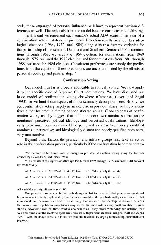
To this end we regressed each senator's actual ADA score in the year of a

confirmation vote on state-level presidential election results from our key ideo-

logical elections (1964, 1972, and 1984) along with two dummy variables for

the partisanship of the senator, Democrat and Southern Democrat.9 For nomina-

tions through 1968, we used the 1964 election; for nominations from 1969

through 1975, we used the 1972 election; and for nominations from 1981 through

1988, we used the 1984 election. Constituent preferences are simply the predic-

tions from the equation. These predictions are uncontaminated by the effects of

personal ideology and partisanship. '0

Confirmation Voting

Our model thus far is broadly applicable to roll call voting. We now apply

it to the specific case of Supreme Court nominations. We have discussed our

basic model of confirmation voting elsewhere (Cameron, Cover, and Segal 1990), so we limit those aspects of it to a summary description here. Briefly, we

see confirmation voting largely as an exercise in position taking, with few incen-

tives either for credit claiming or sophisticated voting. Close students of confir-

mation voting usually suggest that public concern over nominees turns on the

nominees' perceived judicial ideology and perceived qualifications. Ideologi-

cally proximate nominees should be perceived as attractive; poorly qualified

nominees, unattractive; and ideologically distant and poorly qualified nominees,

very unattractive.

Beyond these factors the president and interest groups may take an active

role in the confirmation process, particularly if the confirmation becomes contro-

9We controlled for home state advantage in presidential election voting using the formula

derived by Lewis-Beck and Rice (1983).

'The results of the regressions through 1968. from 1969 through 1975, and from 1981 forward

are respectively

ADA = 27.3 + .95*DVote + 42.3XDem - 25.7*SDem, adj R' = .49;

ADA = 35.3 + 2.4*DVote + 37.5*Dem - 21.01 SDem, adj R' = .58;

ADA = 29.5 + 2.1*DVote + 49.5*Dem - 21.4lSDem, adj R' = .69.

All variables are significant at p < .05.

One potential problem with this methodology is that to the extent that pure representational

behavior is not entirely explained by our predictor variables, the residuals will pick up some of that

representational behavior and treat it as shirking. For instance, the ideological distance between

Democratic and Republican constituents may not be the same within every southern state. Similar

studies, however, show that these residuals do behave as if they measure shirking; for instance, they

wax and wane over the electoral cycle and correlate with previous electoral margins (Kalt and Zupan

1990). With the above caveats in mind. we treat the residuals as largely representing nonconstituent

interests.


io6 Jeffrey A. Segal, Charles M. Cameron, and Albert D. Cover

versial. The president will generally have more political resources to deploy and

can deploy these resources more effectively when his party controls the Senate

and when he is not in the fourth year of his term. In addition, presidential resources are likely to have a greater impact on members of his own party than on

senators of the other party (Massaro 1990). Finally, we include the president's

popularity, which has been extensively linked to executive success in the legis-

lative arena (Edwards 1980, 1989; Kernell 1986; Mouw and MacKuen 1989;

Neustadt 1960; Ostrom and Simon 1985; Rivers and Rose 1985; Rohde and

Simon 1985). Next, we account for the fact that organized interest groups, rep-

resenting, as they do, more active citizens and potential campaign contributions,

might also be able to influence senators. Certainly, there is historical evidence

that lobbying campaigns have influenced the confirmation process. For example,

Fish (1989) argues that the rejection of Judge Parker in 1930 was due in large

part to the activity of organized labor and the NAACP in mobilizing opposition to the nomination. The nomination of Haynsworth brought forth a torrent of

interest group activity, which in turn was exceeded by the almost frenetic mobi-

lization of groups during the Bork nomination.

Despite the importance of group activity in these and possibly other nomi-

nations, almost no systematic empirical work has been undertaken on the role of

interest groups in nominations to the Supreme Court (but see Caldeira and

Wright 1989). In fact, while numerous scholars have, with mixed results, examined the motivation and consequences of campaign contributions by organized groups (Austin-Smith 1987; Baron 1989; Chappell 1982; Denzau and

Munger 1986; Jacobson 1987; Welch 1974; J. Wright 1985), very few studies systematically gauge the effect of lobbying on legislators' votes or governmental

decisions (see Schlozman and Tierney 1986, chap. 12; J. Wright 1990). Surpris-

ingly, there is more systematic evidence of the influence of organized interests

on the judicial process (Caldeira and Wright 1988; O'Connor and Epstein 1983; Puro 1971).

Data and Variables

Dependent Variable

The dependent variable consists of the 1,475 confirmation votes cast by

senators from the nomination of John Harlan through the nomination of Anthony Kennedy. We exclude nominees approved by voice votes on theoretical and em-

pirical grounds. Theoretically, senators convey no information about their ideo-

logical brand name to constituents when nominees are approved by voice votes.

The only information conveyed is that less than a "sufficient second," one-fifth

of those senators present, desired their votes to be recorded. Empirically, there is no way to be certain how particular senators would have voted. Combing the

Congressional Record for statements of opposition will certainly capture inten-

tions of loquacious senators but will likely miss some quieter senators who might



have voted no. Yet by excluding voice votes, we create a selection bias that might

adversely affect our results. Fortunately, as we demonstrate below, our results

hold whether or not voice votes are included.

Nominee Ideology and Qualifications

To determine perceptions of nominees' qualifications and judicial philoso-

phy, we conducted a content analysis of statements from newspaper editorials

from the time of the nomination by the president until the vote by the Senate.

We selected four of the nation's leading papers, two with a liberal stance (New

York Times and Washington Post) and two with a more conservative outlook

(Chicago Tribune and Los Angeles Times). The results are reported in Table 1.

Table 1. Nominee Margin, Vote Status, Ideology, and Qualifications

President's Margin Qualifi- Nominee Statusa cations

Warren 1954 Strong Voice .74 .75

Harlan 1955 Weak 71-11 .86 .88

Brennan 1957 Weak Voice 1.00 1.00 Whittaker 1957 Weak Voice 1.00 .50

Stewart 1959 Weak 70- 17 1.00 .75 White 1962 Strong Voice .50 .50

Goldberg 1962 Strong Voice .92 .75 Fortas, 1 1965 Strong Voice 1.00 1.00

Marshall 1967 Strong 69-11 .84 1.00

Fortas, 2 1968 Weak 45-43h .64 .85 Burger 1969 Weak 74-3 .96 .12

Haynsworth 1969 Weak 45-55 .34 .16

Carswell 1970 Weak 45-51 .11 .04

Blackmun 1970 Weak 94-0 .97 .12

Powell 1971 Weak 89-1 1.00 .17

Rehnquist, 1 1971 Weak 68-26 .89 .05

Stevens 1975 Weak 98-0 .96 .25

O'Connor 1981 Strong 99-0 1.00 .48 Rehnquist, 2 1986 Strong 65-33 .40 .05

Scalia 1986 Strong 98-0 1.00 .00

Bork 1987 Weak 42-58 .79 .10

Kennedy 1988 Weak 97-0 .89 .37

aThe president is labeled strong in a nonelection year in which the president's party controls the

Senate and weak otherwise.

bVote on cloture-failed to receive necessary two-thirds majority.

Qualifications are measured from 0.00 (least qualified) to 1.00 (most qualified). Ideology is

measured from 0.00 (most conservative) to 1.00 (most liberal).


io8 Jeffrey A. Segal, Charles M. Cameron, and Albert D. Cover

Qualifications ranges from zero (most unqualified) to one (most qualified). Ide-

ology ranges from zero (extremely conservative) to one (extremely liberal). As indicated elsewhere (Cameron, Cover, and Segal 1990), the data are

reliable and appear to be valid. The ideology scores meet the strictest test for

validity, predictive validity. The ideology scores correlate at .80 with the ideo-

logical direction of the votes the approved nominees later cast on the court (Segal

and Cover 1989).

Constituent Ideology

As already noted, we measure constituent ideology as the predictions from

regressing ADA scores on presidential election voting and partisanship.

Constituent Distance

Constituent distance is the squared distance between nominee ideology and constituent ideology. The scaling procedure employed is discussed in Appendix A.

Personal Ideology

We measure each senator's personal "ideology" as the difference between

his or her actual and predicted ADA scores. As discussed above, we make two

predictions about the effect of the residuals. We expect cases 1 and 2 ("Shirk + ")

to be positive and case 3 ("Shirk - ") to be negative.

Presidential Strength and Same Party Status

We measured presidential strength as a dummy variable that takes the value

one when the president's party controls the Senate and the president is not in the

fourth year of his term and zero otherwise. We measured same party as a dummy

variable that takes the value one when a senator is of the same party as the

president and zero otherwise.

Presidential Popularity

We measure the president's popularity as the percentage of people who ap-

prove of the job the incumbent is doing as president as measured by the Gallup survey prior to the Senate vote.

Interest Group Activity

In the best of all possible situations, we would have senator-level data on

the amount of lobbying by organized interests dating back to 1954. Obviously,

such data are unavailable. Thus, while recognizing that some senators will be

lobbied more than others, we choose a variable that measures lobbying activity

with respect to each nominee, the number of organized interests presenting tes-

timony for (interest group pro) and against the nominee (interest group con) at

the Senate Judiciary Committee hearings. Presumably, the more organized op-


A SPATIAL MODEL OF ROLL CALL VOTING lO9

Table 2. Dependent and Independent Variables

Variable Mean Minimum Maximum Std. Dev.

Vote .79 0.00 1.00 .41

Distance .14 .00 .65 .12

Qualifications (lack of) .22 .00 .89 .27

Qualifications x distance .03 .00 .47 .05

Shirk + .08 .00 .69 .12

Shirk - .09 .00 .75 .13

Strong president .25 .00 1 .00 .43

Presidential popularity 54.90 40.00 70.00 9.22

Same party .48 .00 1.00 .50

Interest group + 5.96 .00 2i.00 6.50

Interest group - 6.15 .00 17.00 5.87

position to a nominee, the less support he or she will have, and alternatively, the

more organized support for a nominee, the more support he or she will have.

We have gathered data on nominee ideology and qualifications, presidential

strength and popularity, interest group activity, and senators' personal and con-

stituent ideologies for the 16 nominations from John Harlan to Anthony Kennedy

in order to study the 1,475 confirmation votes cast by senators in those nomina-

tions. We supply additional information on the nominees in Table 1. The variables are summarized in Table 2.

Results

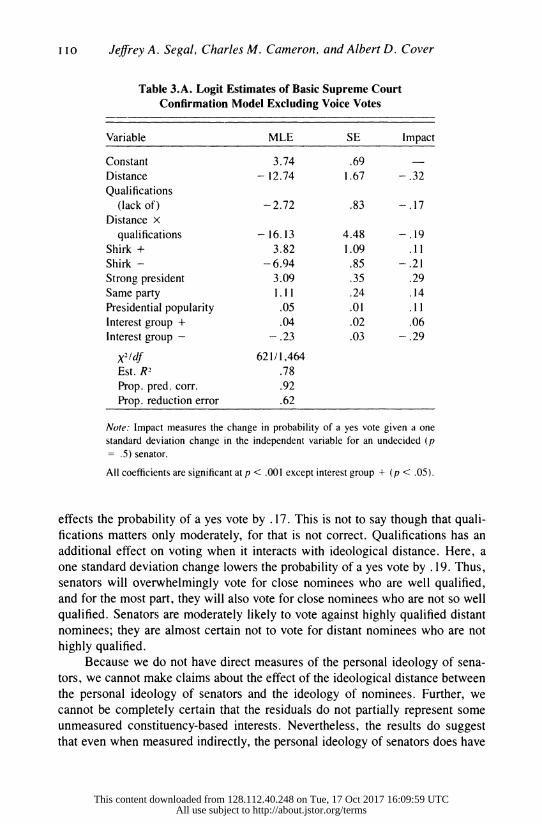
We estimated the model using logit analysis. The results are presented in

Table 3.A. (The essentially similar estimates for the model with voice votes

included is presented in Table 3.B.) As can be seen, the results for the model are

quite impressive. All of the estimated logit coefficients were of the predicted sign, were of reasonable magnitudes, and were highly significant. Ninety-two percent of the votes were predicted correctly, for a 62% reduction in error.

Though logit does not have a commonly accepted R2, the estimated R2 running

the model with the McKelvey-Zavoina probit program is .78." Judged by an

array of statistical criteria, the model was very successful. As the results indicate, confirmation voting is decisively affected by the

ideological distance between senators' constituents and nominees. A one stan-

dard deviation increase in that distance decreases the probability of a yes vote by .32. Qualifications by itself has only a moderate effect on voting. A one standard deviation change in this variable, which accounts for a full quarter of the scale,

"The correlation between the probit and logit estimates is greater than .99.


IIO Jeffrey A. Segal, Charles M. Cameron, and Albert D. Cover

Table 3.A. Logit Estimates of Basic Supreme Court

Confirmation Model Excluding Voice Votes

Variable MLE SE Impact

Constant 3.74 .69

Distance -12.74 1.67 -.32

Qualifications

(lack of) - 2.72 .83 -.17

Distance x

qualifications -16.13 4.48 -.19

Shirk + 3.82 1.09 .11

Shirk - -6.94 .85 - .21

Strong president 3.09 .35 .29

Same party 1.11 .24 .14

Presidential popularity .05 .01 .11

Interest group + .04 .02 .06

Interest group - - .23 .03 -.29

X21df 621/1,464 Est. R2 .78

Prop. pred. corr. .92

Prop. reduction error .62

Note: Impact measures the change in probability of a yes vote given a one

standard deviation change in the independent variable for an undecided (p

= .5) senator.

All coefficients are significant at p < .001 except interest group + (p < .05).

effects the probability of a yes vote by .17. This is not to say though that quali-

fications matters only moderately, for that is not correct. Qualifications has an

additional effect on voting when it interacts with ideological distance. Here, a one standard deviation change lowers the probability of a yes vote by . 19. Thus,

senators will overwhelmingly vote for close nominees who are well qualified,

and for the most part, they will also vote for close nominees who are not so well qualified. Senators are moderately likely to vote against highly qualified distant

nominees; they are almost certain not to vote for distant nominees who are not

highly qualified.

Because we do not have direct measures of the personal ideology of sena-

tors, we cannot make claims about the effect of the ideological distance between the personal ideology of senators and the ideology of nominees. Further, we

cannot be completely certain that the residuals do not partially represent some

unmeasured constituency-based interests. Nevertheless, the results do suggest

that even when measured indirectly, the personal ideology of senators does have


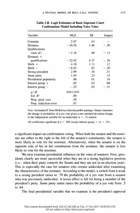
A SPATIAL MODEL OF ROLL CALL VOTING III

Table 3.B. Logit Estimates of Basic Supreme Court

Confirmation Model Including Voice Votes


Constant 2.87 .63

Distance -10.56 1.44 -.30

Qualifications

(lack of) - 2.16 .80 - .13

Distance x

qualifications -22.62 4.27 - .26

Shirk + 4.18 1.11 .12

Shirk - -6.63 .82 - .20

Strong president 2.99 .34 .31

Same party 1.05 .23 .13



Interest group - - .25 .03 - .31

X- /df 636/2,043 Est. R2 .80

Prop. pred. corr. .95


Note: Estimated R2 from McKelvey-Zavoina probit package. Impact measures

the change in probability of a yes vote given a one standard deviation change

in the independent variable for an undecided (p = .5) senator.

All coefficients significant at p < .001 except interest group + (p = .01).

a significant impact on confirmation voting. When both the senator and the nomi-

nee are either to the right or the left of the senator's constituents, the senator is

more likely to vote for the nominee. Alternatively, when the senator is on the

opposite side of his or her constituents from the nominee, the senator is less

likely to vote for the nominee.

We next examine presidential influence on the votes of senators. First, pres-

idents clearly are more successful when they are in a strong legislative position

(i.e., when their party controls the Senate and they are not in an election year).

This is especially the case for senators who remain undecided after examining

the characteristics of the nominee. According to the model, a switch from a weak

to a strong president raises to .79 the probability of a yes vote from a senator

who was previously undecided. A lesser effect is felt for being a member of the

president's party. Same party status raises the probability of a yes vote from .5 to .64.

The final presidential variable that we examine is the president's approval



rating. Unquestionably, there is no one-to-one relationship between presidential

popularity and confirmation approvals. President Nixon, for instance, was at the

height of his popularity when Haynsworth and Carswell were rejected (65% and

63% approval, respectively). President Johnson's approval rating was only at 39% when Thurgood Marshall was confirmed. Yet it is also true that Johnson's

approval ratings were almost as low when Fortas was rejected as chief justice (42%), and President Reagan was near his second-term low when Bork was

defeated (50%). On average, the difference between an unpopular president

(e.g., 40% approval) and a popular one (e.g., 60% approval) is the difference

for an undecided senator between a .50 probability of voting yes and a .77 proba-

bility of voting yes.

Finally, strong interest group mobilization against a nominee can hurt a

candidate, while interest group mobilization for a nominee can have substan-

tively slight but statistically significant positive effects. The Bork nomination

provides an interesting example. Seventeen organized groups provided testimony

against Bork at the Judiciary Committee hearings; 20 provided testimony for him. The net effect was to lower the log of the odds ratio of a yes vote by 3.11.

In probabilistic terms, a moderate-to-conservative southern senator who might have voted for Bork with a probability of .99 without any interest group pressure

would have a probability of voting for him of .60 after the intensive interest

group mobilization.

Interest groups appear to have had an even more devastating effect on the Haynsworth nomination. Sixteen groups presented testimony against Hayn-

sworth; only three presented testimony for him. The net effect was to lower the

log of the odds ratio of a yes vote by 3.85. Senators who would have had a .99

probability of voting for the judge without any interest group involvement would

lean against confirmation (p = .43) after the lobbying campaign. Though many

conservatives blamed the Reagan White House for failing to mobilize support

for Bork, it would seem the Nixon White House was far more "culpable" in its

failure to organize support for Haynsworth.

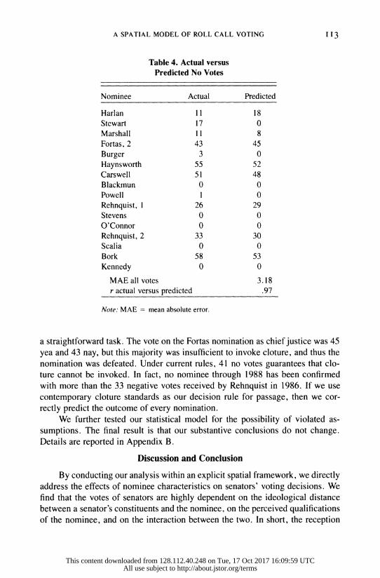
Beyond the parameter estimates, the model does an admirable job in pre-

dicting confirmation outcomes. Table 4 presents the actual and predicted no votes

for every confirmation from John Harlan (1955) through Anthony Kennedy (1988).

Overall, the mean absolute error of the model is but 3.18 votes per confirmation. The correlation between actual and predicted no votes is .97. On a

nomination-level basis, the model overpredicts opposition to the Harlan nomination and underpredicts opposition to Stewart and Bork nominations. All other

nominations are within three votes of predicted totals. This, it should be stressed, is accomplished without any dummy variables for particular nominations that

would prevent out-of-sample predictions.

Gauging the success of the model in terms of confirmation outcomes is not



Table 4. Actual versus

Predicted No Votes

Nominee Actual Predicted

Harlan 11 1 8

Stewart 17 0

Marshall 11 8

Fortas, 2 43 45

Burger 3 0

Haynsworth 55 52

Carswell 51 48

Blackmun 0 0

Powell 1 0

Rehnquist, 1 26 29

Stevens 0 0

O'Connor 0 0

Rehnquist, 2 33 30

Scalia 0 0

Bork 58 53

Kennedy 0 0

MAE all votes 3.18

r actual versus predicted .97

Note: MAE = mean absolute error.

a straightforward task. The vote on the Fortas nomination as chief justice was 45

yea and 43 nay, but this majority was insufficient to invoke cloture, and thus the

nomination was defeated. Under current rules, 41 no votes guarantees that clo-

ture cannot be invoked. In fact, no nominee through 1988 has been confirmed with more than the 33 negative votes received by Rehnquist in 1986. If we use

contemporary cloture standards as our decision rule for passage, then we cor-

rectly predict the outcome of every nomination.

We further tested our statistical model for the possibility of violated as-

sumptions. The final result is that our substantive conclusions do not change.

Details are reported in Appendix B.

Discussion and Conclusion

By conducting our analysis within an explicit spatial framework, we directly

address the effects of nominee characteristics on senators' voting decisions. We

find that the votes of senators are highly dependent on the ideological distance

between a senator's constituents and the nominee, on the perceived qualifications

of the nominee, and on the interaction between the two. In short, the reception



of a nominee depends in a fairly subtle way on the characteristics of the nominee

and the detailed composition of the Senate.

The spatial framework also allows us to address questions of representation

more directly than similar studies of roll call voting. As noted earlier, inferences

about representation are clouded by the use of a residual to measure personal

ideology. In addition, we view representation as more complex than simple

policy congruence. Instead, senators may try to maintain optimal policy reputa-

tions across a range of issues. We suggest this behavior is compatible with a

strong form of representation. Starting with this view of representation, we find

that the individual policy preferences of senators in fact have a measurable

impact on their votes for Supreme Court nominees. This finding indicates

some degree of nonrepresentational behavior, even under a looser concept of

representation.

Finally, we find that the context of a nomination strongly influences roll call

votes. The strength and popularity of the president emerge as important deter-

minants of individual votes. In addition, the relative mobilization of interest

groups around a nominee can have a profound effect on voting.

We close by noting that no analysis, including our own, has done a fully

satisfactory job of incorporating the disparate factors involved in roll call voting.

This is because roll call votes are merely the final (or perhaps the penultimate)

stage in a complex policy process. For example, we consider the ideology and

qualifications of nominees and the mobilization of interest groups to be exoge- nous. However, from a broader perspective, presidents probably pick nominees with an eye toward the entire process, including their chance of confirmation and

impact on the Court. Similarly, interest groups may mobilize for a variety of

reasons. Hence, from a more inclusive perspective, nominee characteristics and

group mobilization should be considered endogenous. This is simple to say; the

difficulty lies in conceptualizing and developing a system of equations to de-

scribe the entire confirmation process. We know of no studies of roll call voting

that adequately resolve this problem (although VanDoren 1990 is clearly in this

spirit). Accordingly, attempts to address an entire policy process, such as the confirmation process, could well prove a fruitful departure for future studies of roll call voting.

Manuscript submitted 30 March 1990

Final manuscript received 28 March 1991

APPENDIX A

We suggested in the text that politicians have preferences over policy reputations, that there is

likely to be a function relating points in reputation space with points in nominee characteristics space,

and that therefore politicians have induced preferences over nominee characteristics. In this appendix



we make this argument more precise and suggest a method for approximating the conversion function

between reputation space and characteristics space.

Preferences and Conversion Function

Let X = (0, II and Y = (0, II be the reputation and characteristics spaces, respectively. Let t,: X -- Y be a continuous and one-to-one (but not necessarily an onto) function. Index the elements of X and Y so that y; = j(x;).

This setup is meant to have the following interpretation: X is a scale indicating senators' policy

brand names; Y is a scale indicating nominee judicial ideology, as perceived by senators; k5 maps

points in X into points in Y for senator i. The c/, function thus acts somewhat like the predictive mappings in Enelow and Hinich ( 1990); given a reputation, senator i understands the location of the

corresponding nominee ideology. We assume the k, functions are identical for all senators so that at any given time liberal and conservative senators have a common understanding of their best corre-

sponding nominee. We therefore drop the subscript on k.

Let W: [0, I1 x [0, I1 -* R be a continuous utility function so that (xj, x-) )-* W(x,; x,). This function is assumed unimodal at x; = x;. In other words, senators have preferences over policy brand

names with senator i's ideal brand name being the point x,. An example of such a function is W =

- (x; - X)2. As discussed earlier, we view this (indirect) "utility" function as induced in senators

by voter choices over candidates with different policy reputations, but we do not explicitly model

how this process works.

Now define the induced utility function in Y as V = W(G(xj), k(-j)) = V(xj, T). For instance, in terms of the earlier example, W = - [4(xj) - 5(X-)]2. Let "a >, b" indicate "a is preferred to b by i." Then x, >, xk iff V(x,; x-) > V(x; x,) iff W(4(xj); 4-,)) > W(C(xk); C(x,)) if 4Cxi) >, k(x,) iff y, >, vw. In other words, preferences can be considered equally well in terms of the original

utility function or of the induced one. In addition, since 4(x,) = y, and C(xk) = Yk, we may consider senator i's preferences entirely in terms of V(v,; k(1-)) and V(vy; 4x,)), provided we know k().'2 This is the approach actually taken in the text.

One could extend this basic framework to develop a theory of measurement error in this setting

(e.g., elements of X map with error into ADA score and elements of Y map with error into nominee

ideology score). Given the statistical results on errors-in-variables reported below, we do not pursue

this point any further.

Estimating a Conversion Function

We now outline a procedure for estimating the conversion function 5, given a general func-

tional form. It is easy to show that a wide range of mappings from nominee ideology space to brand

name space implies a conversion function k -' of the general form g(y,) = 6,h(x,) - 6o. As discussed in the body of this paper, assume a random utility model of voting and a utility function with

the specific functional form presented there. Further assume a squared Euclidean distance as a dis-

tance metric. Then one may search for the values of 65 and 6, that minimize - 2*log likelihood ratio in the logistic regression model; this procedure is somewhat analogous to the Hildreth-Lu procedure

for autocorrelation. Using this method, we derive the conversion function v, = .2 + .5x,. (Note that

this function is continuous and one-to-one [though not onto] as required above.) However, a striking

2The exposition of the random utility model assumed a comparison between the utility of a

nominee and a threshold utility, while the discussion here assumes a comparison between two nom-

inees, j and k. But from the intermediate value theorem and given the assumptions above, for any attainable utility level, there is a corresponding xi. Hence, a politician voting for j if the utility of doing so exceeds a threshold can be treated as if he or she were comparing j with some nominee k

who yields the threshold level of utility.


iI6 Jeffrey A. Segal, Charles M. Cameron, and Albert D. Cover

feature of the data set is the robustness of the qualitative results to a wide range of conversion

parameters. For example, the simplest conversion (8o = 0, 6, = I) fits the data virtually as well as the best conversion and yields fairly similar estimates for the logit parameters.

APPENDIX B

In this appendix we examine our statistical model for any possibilities of violated assumptions.

Specifically, we consider the consequences of measurement error and correlated error structures.

Measurement Error

In deriving our spatial model, we paid careful attention to placing nominee ideology and

senators' preferences in the same policy space. Yet this procedure does not guarantee that either

nominee ideology or senators' preferences are measured without error. The result is that our ideo-

logical distance measure has two potential sources of error. If this error is significant, our parameter

estimates could be biased.

While we accept that some degree of measurement error exists in our data, we do not believe

the amount of error or the resulting bias to be serious. To test this proposition, we conducted reverse

regressions (Klepper and Leamer 1984; Leamer 1984) in which distance and the qualifications-

distance interaction become the left-hand-side variables, and vote is placed on the right-hand-side of

the equation. In neither instance do we find the systematic effects of measurement error that are

found, for example, in employment discrimination analyses (Maddala 1988).

Correlated Error Structures

Because of the pooled cross-sectional time series design of the study, there are three distinct

ways in which errors can be correlated with one another: over time, over space, and over both time

and space (Stimson 1985). Correlations over time would be most likely to exist if the error of a

particular senator at time t correlated with the error of that senator at any time beyond t. Correlations

over space would be most likely to occur if the errors of one or more senators on a particular vote

correlate with the errors of other senators on that same vote. For instance, our residual analysis

suggests that we consistently overpredicted the probability of voting in favor of Potter Stewart (see

Table 4). Correlations over time and space would occur if the true slope coefficients vary from one

nomination to another.

To control for the possibility of correlated errors in time and space, we employed a logit variant

of the least squares dummy variable technique (Sayrs 1989). First, to control for correlations across

time, we added a dummy variable for the 234 senators who voted in more than one confirmation.

The results suggest that autocorrelated errors are not a problem; the senator dummies taken as a

whole were not significant at p < .20.

The more likely problem, as noted above, is correlation across space, or heteroscedasticity.

We therefore attempted to include a dummy variable for all but one of the nominees, but extremely

high multicollinearity between subsets of the nominee dummies and some of the nominee-level vari-

ables prevented the equation from being estimated. Since we could not enter the complete set of

nominee dummies, we chose to enter those in which the model mispredicted the total number of no

votes by more than three, for here it is most likely that we shall have correlated errors across senators.

The results are presented in Table 5.

As can be seen, the new model does significantly improve the overall fit. The X' drops from 621 to 517 with only three additional degrees of freedom. The mean absolute error of predicted no votes drops to 2.1 per confirmation. The percentage predicted correctly barely improves though,

increasing from 92.1 to 93.5. Most important, there is virtually no change in the substantive inter-



Table 5. Logit Estimates of Dummy Variable Supreme Court

Confirmation Model


Constant 6.69 1.26

Distance - 16.00 2.20 - .37

Qualifications

(lack of) - 3.89 1.10 -.24

Distance x

qualifications - 19.22 5.53 -.23

Shirk + 4.29 1.24 .13

Shirk - -7.68 .96 - .23 Strong president 3.50 .49 .32

Same party 1.00 .27 .12



Interest group - - .23 .04 - .29

Harlan 1.59 .83

Stewart - 3.60 .69 -

Bork - 2.88 1.15

X-ldf 517/1.461 Prop. pred. corr. .93


Note: Impact measures the change in probability of a yes vote given a

one standard deviation change in the independent variable for an unde-

cided (p = .5) senator.

All substantive coefficients significant at p < .001 except popularity (not

significant) and interest group + (p = .05). Stewart and Bork signifi-

cant at p < .01 Harlan, at p = .05.

pretations of the coefficients. With the exception of presidential popularity, significance levels remain

extremely high, and the impact of the variables, though changed somewhat, are relatively the same.'3

One significant difference is the greater effect of positive interest group mobilization, but that still pales in comparison to negative interest group mobilization. 14

If the slope coefficients for the independent variables vary for each nomination, then the model

will produce correlated errors in time and space. The usual method of estimating the extent of such

problems is to run separate logit analyses for each nomination and then use a x2 test to determine

whether restricting the coefficients to the same value across nominations (i.e., pooling) results in a

significant reduction in overall fit (Sayrs 1989). Unfortunately, the nature of our data makes such a

"Presidential popularity remains significant when voice votes are included in the model. 'I4f we add dummy variables for all nominees whose no votes are mispredicted by two votes

or more, multicollinearity starts to become an extreme problem. For instance, the correlation between strong president and the remaining variables in the model increases to .9, and its standard

error jumps from .6 to 2.5. Nevertheless, the parameter estimates remain basically the same.


I I 8 Jeffrey A. Segal, Charles M. Cameron, and Albert D. Cover

test impossible. First, several of the nominations were unanimous, and thus there is no variance to

explain within those cross-sections. We could exclude these cross-sections from our pool but to do

so leaves unexplained why those nominees received such high levels of support relative to other

nominees (presumably because they are ideologically moderate or highly qualified) and simultane-

ously creates a serious selection bias problem. Second, our model necessarily makes use of nominee-

level independent variables such as the qualifications of the nominee. These variables could not be

used to predict votes in individual nominations, as the scores only vary across nominations. Because

of these problems, we then attempted a simpler test to determine whether the slope for ideological

distance varies across nominations by including interaction terms between each of the N - I nomi-

nees and ideological distance. Unfortunately, the logit results did not converge. We were able to test

whether the slope for ideological distance differed from the first eight nominations to the next eight

by adding a dummy variable for the first set and an interaction between the dummy variable and

ideological distance. Neither estimate was even close to being significant. The results though are

only a necessary condition for assuming constant slopes, not a sufficient condition.

We are left without an explicit test of whether the nominations should be pooled. We note

though that the case for pooling is at least reasonable given the overall fit of the model. It is difficult

to imagine that we could predict 93% of the votes correctly and obtain a mean absolute error of 2.1

votes per nomination if the slope coefficients across nominations are randomly distributed. '"

REFERENCES

Achen, Christopher H. 1978. "Measuring Representation." American Journal of Political Science

22:475-510.

. 1986. The Statistical Analysis of Quasi-Experiments. Berkeley: University of California

Press.

Arnold, R. Douglas. 1990. The Logic of Congressional Action. New Haven: Yale University Press.

Austin-Smith, David. 1987. "Interest Groups, Campaign Contributions, and Probabilistic Voting."

Public Choice 54: 123-39.

Baron, David P. 1989. "Service-induced Campaign Contributions and the Electoral Equilibrium." Journal of Economics 104:45-72.

Baumol, William, John Panzar, and Robert Willig. 1982. Contestable Markets and the Theory of Industry Structure. New York: Harcourt Brace Jovanovich.

Bernstein, Robert, and Stephen R. Horn. 1981. "Explaining House Voting on Energy Policy: Ide-

ology and the Conditional Effects of Party and District Economic Interests." Western Political

Quarterly 34:235-45.

Caldeira, Gregory A., and John Wright. 1988. "Organized Interests and Agenda Setting in the U.S.

Supreme Court." American Political Science Review 82: 1109-28.

. 1989. "Organized Interests before the Senate: The Politics of Federal Judicial Nomina-

tions." Presented at the annual meeting of the Law and Society Association, Madison, WI.

. 1990. "Amici Curiae before the Supreme Court: Who Participates, When, and How

Much?" Journal of Politics 52:782-806.

Cameron, Charles, Albert Cover, and Jeffrey Segal. 1990. "Senate Voting on Supreme Court Nom-

inees: A Neoinstitutional Model." American Political Science Review 84:525-34.

Carson, Richard A., and Joe Oppenheimer. 1984. "A Method of Estimating the Personal Ideology

of Political Representatives." American Political Science Review 78: 163-78.

Chappell, Henry W. 1982. "Campaign Contributions and Congressional Voting: A Simultaneous

Probit-Logit Model." Review of Economics and Statistics 64:77-83.

" Wallace (1972) shows that even in circumstances where coefficients do differ between differ-

ent cross-sections, pooling can lead to more precise estimates than the individual estimator variances.


A SPATIAL MODEL OF ROLL CALL VOTING II9

Collie, Melissa P. 1984. "Voting Behavior in Legislatures." Legislative Studies 9:3-50.

Denzau, Arthur, and Michael Munger. 1986. "Legislators and Interest Groups: How Unorganized

Interests Get Represented." American Political Science Review 80: 89- 106.

Denzau, Arthur, William Riker, and Kenneth Shepsle. 1985. "Farquharson and Fenno: Sophisticated

Voting and Homestyle. " American Political Science Review 79: 1117-34.

Dougan, William R., and Michael C. Munger. 1989. "The Rationality of Ideology." Journal of Law

and Economics 32: 119-42.

Downs, Anthony. 1957. An Economic Theorv of Democracv. New York: Harper and Row.

Edwards, George C. 1989. At the Margins: Presidential Leadership of Congress. New Haven: Yale

University Press.

Enelow, James, and Melvin Hinich. 1982. "Nonspatial Candidate Characteristics and Electoral

Competition. Journal of Politics 44: 115- 30.

. 1984. The Spatial TheorY of Voting: An Introduction. New York: Cambridge University Press.

. 1990. "The Theory of Predictive Mappings." In Advances in the Spatial Theory of Voting,

ed. James Enelow and Melvin Hinich. New York: Cambridge University Press.

Felice, John D., and Herbert F. Weisberg. 1988. "The Changing Importance of Ideology, Party, and

Region in Confirmation of Supreme Court Nominees, 1953-88.' Kentuckv Law Journal

77:509-31.

Fenno, Richard. 1973. Congressmen in Committees. Boston: Little, Brown.

1978. Home Stvle: House Members in Their Districts. Boston: Little, Brown.

Fiorina, Morris P. 1974. Representatives, Roll Calls, and Constituencies. Lexington, MA: Heath.

Fish, Peter G. 1989. "Spite Nominations to the United States Supreme Court: Herbert Hoover, Owen

J. Roberts, and the Politics of Presidential Vengeance in Retrospect." Kentucky Law Journal

77:545-76.

Jacobson, Gary C. 1987. The Politics of Congressional Elections. 2d ed. Boston: Little, Brown.

Kalt, Joseph P. 1981. The Economics and Politics of Oil Price Regulation. Cambridge: MIT Press.

Kalt, Joseph P., and Mark A. Zupan. 1984. "Capture and Ideology in the Economic Theory of Politics. American Economic Review 74:279-300.

. 1990. "The Apparent Ideological Behavior of Legislators: Testing for Principal-Agent Slack

in Political Institutions." Journal of Law and Economics 33: 103-31.

Kau, James B., and Paul H. Rubin. 1979. "Self-Interest, Ideology, and Logrolling in Congressional

Voting. " Journal of Law and Economics 22: 365- 84.

. 1982. Congressmen, Constituents, and Contributors. Boston: Martinus Nijhoff.

Kernell, Samuel. 1986. Going Public: New Strategies of Presidential Leadership. Washington, DC:

Congressional Quarterly Press.

Key, V. 0. 1967. Public Opinion and American Democrac v. New York: Knopf.

Klepper, S., and Edward E. Leamer. 1984. "Consistent Sets of Estimates for Regressions with Errors

in All Variables." Econometrica 52: 163-83.

Krantz, David H., and Amos Tversky. 1971. "Conjoint-measurement Analysis of Composition

Rules in Psychology." Psychological Review 78: 151- 69.

Krehbiel, Keith. 1988. "Spatial Models of Legislative Choice." Legislative Studies 13:259-321.

Krehbiel, Keith, and Douglas Rivers. 1988. "The Analysis of Committee Power: An Applica-

tion to Senate Voting on the Minimum Wage." American Journal of Political Science 32:

1151-74.

Leamer, Edward E. 1984. Sources of International Comparative Advantage: Theory and Evidence.

Cambridge: MIT Press.

Lewis-Beck, Michael, and Tom Rice. 1983. "Localism in Presidential Elections: The Home State

Advantage." American Journal of Political Science 27:548-56.

Louviere, Jordan J. 1988. Analyzing Decision Making: Metric Conjoint Analysis. Beverly Hills: Sage.



Macdonald, Stuart Elaine, and George Rabinowitz. 1987. "The Dynamics of Structural Realign-

ment." American Political Science Review 81: 775-96.

MacRae, Duncan. 1970. Issues and Parties in Legislative Voting: Methods of Statistical Analysis.

New York: Harper and Row.

Maddala, G. S. 1988. Introduction to Econometrics. New York: Macmillan.

Massaro, John. 1990. Supremelv Political. Albany: State University of New York Press.

Mayhew, David. 1974. Congress: The Electoral Connection. New Haven: Yale University Press.

Miller, Warren, and Donald Stokes. 1963. "Constituency Influence in Congress." American Politi-

cal Science Review 57: 45- 56.

Mouw, Calvin, and Michael MacKuen. 1989. "The Strategic Configuration, Political Influence, and

Presidential Power in Congress." Presented at the annual meeting of the Midwest Political

Science Association, Chicago.

Nelson, Douglas, and Eugene Silberberg. 1987. "Ideology and Legislator Shirking." Economic

Inquiry 25: 15-25.

Neustadt, Richard E. 1960. Presidential Power: The Politics of Leadership. New York: Wiley.

O'Connor, Karen, and Lee Epstein. 1983. "The Rise of Conservative Interest Group Litigation."

Journal of Politics 45:479-89.

Ostrom, Charles W., and Dennis M. Simon. 1985. "Promise and Performance: A Dynamic Model

of Presidential Popularity." American Political Science Review 79:349-58.

Peltzman, Sam. 1984. "Constituent Interest and Congressional Voting." Journal of Law and Eco-

nomics 27:181-210.

Pitkin, Hannah F. 1967. The Concept of Representation. Berkeley: University of California Press.

Poole, Keith T. 1988. "Recent Developments in Analytical Models of Voting in the U.S. Congress."

Legislative Studies 13:117-33.

Puro, Stephen. 1971. "The Role of Amicus Curiae in the United States Supreme Court, 1920-

1966." Ph.D. diss., State University of New York, Buffalo.

Rabinowitz, George, and Stuart Elaine Macdonald. 1989. "A Directional Theory of Voting." Ameri-

can Political Science Review 83:93- 122.

Rivers, Douglas, and Nancy Rose. 1985. "Passing the President's Program: Public Opinion and

Presidential Influence in Congress." American Journal of Political Science 29: 183-96.

Rohde, David W., and Dennis M. Simon. 1985. "Presidential Vetoes and Congressional Response:

A Study of Institutional Conflict." American Journal of Political Science 29:397-427.

Rohde, David W., and Harold Spaeth. 1976. Supreme Court Decision Making. San Francisco:

Freeman.

Sayrs, Lois W. 1989. Pooled Time Series Analysis. Beverly Hills: Sage.

Schlozman, Kay L., and John T. Tierney. 1986. Organized Interests and American Democracy. New

York: Harper and Row.

Schneider, Jerrold. 1979. Ideological Coalitions in Congress. Westport, CT: Greenwood Press.

Segal, Jeffrey A., and Albert D. Cover. 1989. "Ideological Values and the Votes of U.S. Supreme

Court Justices." American Political Science Review 83:557-65.

Shapiro, Catherine R., David W. Brady, Richard A. Brody, and John A. Ferejohn. 1990. "Linking

Constituency Opinion and Senate Voting Scores: A Hybrid Explanation." Legislative Studies

15:599-622.

Songer, Donald R. 1979. "The Relevance of Policy Values for the Confirmation of Supreme Court

Nominees." Law and Society Review 13:927-48.

Stimson, James. 1985. "Regression in Space and Time: A Statistical Essay." American Journal of

Political Science 29:914-47.

Train, Kenneth. 1986. Qualitative Choice Analysis: Theorv, Econometrics, and an Application to

Automobile Demand. Cambridge: MIT Press.



Turner, Julius. 1951. Partv and Constituencv: Pressures on Congress. Baltimore: Johns Hopkins

University Press.

VanDoren, Peter M. 1990. "The Limitations of Roll-Call Vote Analysis." Legislative Studies

15:311-40.

Welch, William. 1974. "The Economics of Campaign Funds." Public Choice 20:83-97.

Wright, Gerald C., Robert Erikson, and John Mclver. 1985. "Measuring State Partisanship and

Ideology with Survey Data." Journal of Politics 47:469-89.

Wright, John R. 1985. "PACs, Contributions, and Roll Calls: An Organizational Perspective."

American Political Science Review 79:400- 14.

. 1990. "Contributions, Lobbying, and Committee Voting in the U.S. House of Representa-

tives. " American Political Science Review 84: 417- 38.

Wallace, T. 0. 1972. "Weaker Criteria and Tests for Linear Restrictions in Regression." Econome-

trica 40:689-98.


a spatial model of roll call voting: senators ... spatial model of roll call voting: senators,...

Documents