1

A SPATIAL MODELING FRAMEWORK FOR ANALYZING POTENTIAL EARTHQUAKE DAMAGE:

AN APPLICATION TO MEMPHIS

Tony E. Smith*, Richard L. Bernknopf**, and Anne M. Wein**

May, 2010

Abstract Identifying options and making decisions to reduce natural hazard losses from large earthquakes rely on vulnerability and hazard assessments for a parcel of land, neighborhood, community, or region. These assessments are based on probabilistic estimates of damages; however, the damage probabilities and projections of economic losses contain uncertainties large enough to complicate mitigation policy decisions. The modeling framework developed here extends the use of scientific information for damage estimation by incorporating spatial uncertainties about the earthquake source and local geologic conditions. A well established methodology exists for evaluating probabilistic damage and loss estimates at a site. But what is less understood is how to aggregate site information into a risk analysis for a portfolio of sites (study area). The most straightforward approach is to assume spatially independent damages and losses. However, empirical scientific evidence indicates that levels of shaking and liquefaction at sites close to one another tend to exhibit some degree of positive correlation. While such correlations do not affect the expected losses in a given study area, they do increase the variance (uncertainty) of these losses. We demonstrate these effects in a neighborhood of more than 1,200 land parcels in Memphis, TN, by comparing simulated spatially independent and dependent losses resulting from a 7.7 magnitude earthquake. Repeated simulations on a regional scale yield a sampling distribution of total realized losses provide maximum-likelihood estimates for exceedance probability (EP) functions of loss. A value at risk (VaR) assessment based on these exceedance probabilities is then used to illustrate the effect of spatial uncertainty on a hypothetical mitigation plan decision in a Memphis neighborhood. A comparison of these assessment results for both spatially dependent and independent scenarios shows how a failure to account for unobserved spatial dependencies can lead to an underestimate of potential extreme damage and loss conditions.

* Department of Electrical and Systems Engineering, University of Pennsylvania ** Western Geographic Science Center, US Geological Survey

2

1. Introduction Strategies, policies, and regulations intended to improve human safety and reduce losses from natural hazards affect us individually and collectively. Hazards such as earthquakes, volcanoes, and floods pose widespread and significant risks to many aspects of society. Risk assessment entails the evaluation of information about the historical frequency and severity of previous disasters, anthropogenic and natural environmental vulnerability, and characterization of the indicated risks. Although catastrophes recur over long periods of time, in the short run, there is considerable uncertainty regarding the location and recurrence of severe hazards. In this paper, we focus on the uncertainty about the physical damage from an earthquake of a given magnitude and illustrate the potential effect of spatial autocorrelation on the uncertainties embodied in an earthquake mitigation plan. While it can be accepted that spatial dependencies increase the variability of the economic losses from natural hazards, this has not been explicitly incorporated into probabilistic models for insured losses (Grossi et al, 2005) or analyses of community damages for actual properties (HAZUS, 1997; Goodno et al., 2006; Elnashai et al., 2008). In this paper, a spatially dependent loss model is developed for a single large earthquake with random earthquake source locations. Models of spatially correlated ground motions in earthquake events have been proposed by many authors, including Boore (1997), Wesson and Perkins (2001), Boore et al. (2003), Wang and Takada (2005) and Goda and Hong (2008), among others. The present model focuses on spatially dependent losses to property, and is most closely related to the work of Wesson and Perkins (2001) together with the more recent extensions in Wesson, Perkins and Luco (2009) and Karaca and Luco (2009). In the original (2001) paper a probabilistic model is developed to analyze the annual losses to a portfolio of properties exposed to earthquakes. In particular, they formulate their analysis in terms of exceedance probabilities, which also form the basis for the present approach. In addition, they focus on the increase in loss variance due to inter-event correlations among sites arising from their common exposure to a random series of earthquake events over time. In the more recent 2009 papers there is a more explicit consideration of intra-event effects arising from the common exposure of sites to a given earthquake. But all correlations between sites are again assumed to be generated by inter-event effects. In particular, the ground motion effects at individual sites are assumed to depend only on their distance to the earthquake source, and not their distances to each other. In contrast to this approach, the present paper focuses on correlation effects arising from the continuity properties of seismic waves themselves. More specifically, the spatial dependencies arising from such continuities are here modeled probabilistically in terms of a semivariogram that is similar in spirit to the original spatial correlation model proposed by Boore (1997).1

1 The possibility of such local correlation effects (“directivity” and “basin” effects) is also mentioned in Wesson et al. (2006). But their model focuses on long-run temporal correlations.

3

In the development of the present model, two sources of uncertainty are identified. First, there is uncertainty about the actual likelihood of damage (i.e., about the underlying science of earthquake physics). There is also uncertainty about the costs of damage (i.e., about the proper valuations of assets at risk, such as building value and property value). We consider loss outcomes under two alternative assumptions: (1) spatial independence: damages to distinct land parcels that are statistically independent and, (2) spatial dependence: damages to adjacent parcels are more highly correlated than damages to spatially separated parcels. Our main finding is that the spatially dependent model produces damage distributions with fatter right tails (i.e., higher damage-exceedance probabilities) than the spatially independent model.2 The paper is organized into four sections. Section 2 outlines the basic elements of a probabilistic model that includes spatial dependencies for analyzing the potential damage costs from shaking and liquefaction during large earthquakes. The model is then applied in section 3 to an earthquake hazard scenario involving a magnitude 7.7 earthquake in the New Madrid zone. In particular, the expected damage cost (loss) and dispersion of damage costs (risk) are analyzed for a small portfolio of spatially contiguous properties in Memphis, TN. This example provides a range of damage costs that can be used in a conditional risk-return decision framework. (In the Appendix we outline possible extensions of this cost framework to include the loss of public amenities and other damage costs external to individual parcels.) In section 4, we demonstrate the potential use of this model for policy analysis and industry decision making that involve the assessment of simultaneous multiple risks (Sinn, 1983). In particular, we develop a policy example that illustrates how existence and recognition of spatially correlated losses can change a mitigation choice. In the example, probabilistic damage costs are estimated under alternative model assumptions to assess whether these costs exceed tolerable risks. 2. The Spatially Dependent Model The following model is based on the premise that a Magnitude (M) 7.7 earthquake occurs with source somewhere in the New Madrid seismic zone, as shown roughly by the three lines north of Memphis, TN in Figure 2.1.3

Conditional on this event, the model is designed to estimate total losses,C , for building sites in Memphis, TN. The model decomposes the loss probabilities for a given magnitude earthquake into a probability tree as follows. Denoting the set of possible earthquake sources by{ : 1,.., }ix i n ,4 the conditional distribution of C given M can be

decomposed as follows:

2 Essentially the same result was obtained by Wesson and Perkins (2001) for the case of inter-event correlations. 3 This figure is adapted from Figure 7 in Frankel et al. (1996). 4 This set of earthquake sources is made precise in Section 2.1 below.

Figure 2.1 here

4

(1) 1

Pr( | ) Pr( | , )Pr( | )n

i iiC c M C c x M x M

We refer to the terms, ( | )iP x M as earthquake-source probabilities, and the

terms, ( | , )iP C c x M as conditional-cost probabilities. We now consider the

specification of these two probabilities in more detail. 2.1 Earthquake Source Probabilities The relevant portion of the New Madrid seismic zone is represented by the three “pseudo fault” lines in Figure 2.1 (Frankel et al., 1996). The center line consists of a fault trace matching recent microearthquake activity, and the two outer lines roughly approximate the edges of the Realfoot Rift (Stover and Coffman, 1993). For a large magnitude earthquake event, it is reasonable to postulate that the source is most likely to be located in the vicinity of these three “pseudo fault” lines. Each earthquake event is assumed to be characterized by a rupture along one of these lines. Following Wells and Coppersmith (1994), the Magnitude 7.7 earthquake will yield an expected rupture length of 140 km. Since each “pseudo fault” line in Figure 2.1 is approximately 240 km, we assume that the southern end, x , of the rupture is randomly located in the southern-most 100 km segment of each “pseudo fault” line.5 This earthquake source, x , completely defines an associated rupture event as the 140 km segment extending north from x along the given “pseudo fault” line. It is convenient to represent fault ruptures by their earthquake source. Following Frankel (2005), the analysis is restricted to a discrete set of possible earthquake sources uniformly spaced along the southern end of each “pseudo fault” line as shown schematically by the dots on the center line in Figure 2.1. With the set of earthquake sources on the center line denoted by

00 01 0{ ,.., }nX x x and those on the edge

lines denoted by 1{ ,.., }, 1,2ii i inX x x i [again following Frankel (2005)], it is assumed

that each center-line earthquake source in 0X is twice as likely as each source

in 1 2X X . With these assumptions, the resulting earthquake-source probabilities,

Pr( | )x C , are given by6

(2) 0

1 2

0 1 2

0 1 2

22

12

,Pr( | )

,

n n n

n n n

x Xx M

x X X

2.2 Conditional-loss Probabilities

5 Essentially the same procedure was employed by Wesson and Perkins (2001), who used a Magnitude 7.5 earthquake with an expected rupture length of 100 km along a single representative fault line. 6 While (2) is the specific model is used for the simulations in section 4 below, many refinements of this simple model are of course possible.

5

The conditional-loss probabilities are decomposed in the following manner. For each building (parcel) site, , 1,..,j j m , let the indicator variable, j , denote the destruction

event at site j , with 1j if the structure at site j is destroyed and 0j otherwise.7 In

these terms, the random lossC , is taken to be a sum of the form

(3) 1

m

j jjC c

where jc is the expected building loss when 1j . We consider the specification of

jc and j in turn.

2.2.1 Expected Damage Costs First it should be noted that building loss uncertainty is typically represented in terms of structural-fragility curves (as detailed, for example in HAZUS, 1997).8 However, given the levels of uncertainty already implicit in this earthquake model, it seems reasonable (for our present purposes) to focus only on expected losses, jc , for individual buildings.

These costs will generally depend on the type of failure as well as the particular building type at site j. Here it is assumed that a failure is due to either shaking or shaking-induced liquefaction. (A simplified version focusing only on shaking-induced liquefaction is developed in the example of Section 4.2 below.) The possibility of liquefaction failure at sites j is taken to be summarized by a set of liquefaction probabilities jp .9 Hence, if the

expected losses from shaking and liquefaction at site j are denoted respectively by Sjc and L

jc , then the overall expected damage cost at site j is given by:

(4) ( | , ) (1 )L S

j j i j j j jc E C x M p c p c

Note finally from the additive specification of (3) that each jc is implicitly assumed to

include only those costs directly attributable to damage at site j (i.e., the replacement value or replacement cost of a building at j). 2.2.2 Destruction Probabilities The calculation of the probabilities of destruction events, j , assumes that complete loss

depends only on the peak ground acceleration (PGA), jA , generated at site j by the given

the earthquake. In particular, it is assumed that destruction at site j occurs when some

7 This simplification ignores degrees of destruction, and simply considers full destruction versus no destruction. 8 This approach is also incorporated into the earthquake loss model of Wesson and Perkins (2001). 9 The liquefaction probability data for Memphis is from Rix, G.J. and S. Romero-Hudock (2006).

6

(appropriately chosen) threshold level, ja , of ground acceleration is exceeded. Formally

it is postulated that (5) 1j j jA a

All destruction probabilities are determined by the joint distribution of PGA levels. The joint realization of PGA levels is denoted by the random vector ( : 1,.., )jA A j m .

Following standard practice in seismological modeling, A is assumed to be conditionally distributed as a probabilistic mixture (“logic tree”) of K log normal distributions,10

(6) 2

1ln ( , ),

K

k k i mkA w N x M I

with individual mean vectors, ( , )k ix M , 1,..,k K , and common diagonal covariance

matrix, 2mI . Each component distribution is characterized by its mean vector, usually

designated as its attenuation function, (7) ( , ) [ ( , ) : 1,.., ]k i k ijx M r M j m

where ijr is the closest distance from site j to the “pseudo fault” line rupture represented

by earthquake source ix .11 The attenuation functions are each based on physical theories

of earthquake propagation, and are typically formulated as separable additive functions of r and M :12 (8) 0 1 2 3( , ) lnk k k k kr M M r r

Other attenuation relationships are constructed in tabular form, where PGA values are listed for the appropriate range of distances r , and magnitudes M . The use of model mixtures in expression (6) provides a convenient way to incorporate the high degree of uncertainty that exists regarding the actual PGA levels at a location. 2.3 Spatial Autocorrelation of PGA Levels

10 In practice, the mixture weights,

kw , are often chosen to be uniform ( 1/

kw K ), reflecting the current

lack of consensus among experts as to which models are better in any given situation An explicit example of a logic tree for the New Madrid zone is given in Cramer (2001). See also Frankel et al. (1996, 2002). 11 It should be noted that distance is usually measured to the hypocenter of the quake (reflecting depth as well as surface distance). But following Frankel et al. (1996, 2002) the depth of the quake is here taken to be constant, so that surface distance is the only relevant variable. 12 A more elaborate example (involving “depth” as well as distance) is given in expression (16) below.

7

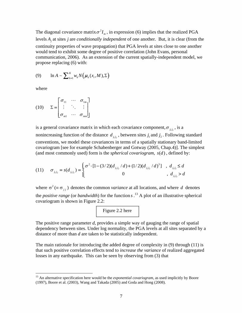
The diagonal covariance matrix 2mI , in expression (6) implies that the realized PGA

levels jA at sites j are conditionally independent of one another. But, it is clear (from the

continuity properties of wave propagation) that PGA levels at sites close to one another would tend to exhibit some degree of positive correlation (John Evans, personal communication, 2006). As an extension of the current spatially-independent model, we propose replacing (6) with:

(9) 1

ln ( , ),K

k k ikA w N x M

where

(10) 11 1

1

m

m mm

is a general covariance matrix in which each covariance component,

1 2j j , is a

nonincreasing function of the distance 1 2j jd , between sites 1j and 2j . Following standard

conventions, we model these covariances in terms of a spatially stationary band-limited covariogram [see for example Schabenberger and Gotway (2005, Chap.4)]. The simplest (and most commonly used) form is the spherical covariogram, ( )s d , defined by:

(11) 1 2 1 2 1 2

1 2 1 2

1 2

2 3[1 (3 / 2)( / ) (1/ 2)( / ) ] ,( )

0 ,

j j j j j j

j j j j

j j

d d d d d ds d

d d

where 2 ( )j j denotes the common variance at all locations, and where d denotes

the positive range (or bandwidth) for the function s .13 A plot of an illustrative spherical covariogram is shown in Figure 2.2:

The positive range parameter d, provides a simple way of gauging the range of spatial dependency between sites. Under log normality, the PGA levels at all sites separated by a distance of more than d are taken to be statistically independent. The main rationale for introducing the added degree of complexity in (9) through (11) is that such positive correlation effects tend to increase the variance of realized aggregated losses in any earthquake. This can be seen by observing from (3) that

13 An alternative specification here would be the exponential covariogram, as used implicitly by Boore (1997), Boore et al. (2003), Wang and Takada (2005) and Goda and Hong (2008).

Figure 2.2 here

8

(12) 1var( | ) var

m

j jjC M c M

2

1 1var( | ) cov( , | )

m m

j j j h j hj j h jc M c c M

The assumption of a diagonal covariance matrix, 2mI , in (6) implicitly assumes that

all covariance terms on the right hand side of (12) are zero. But in the presence of locally positive spatial dependencies (such as in Figure 2.2 above), many of the covariance terms will be positive, which may dramatically increase the overall magnitude of var( | )C M .14 These spatial dependencies thus constitute an important component of the overall uncertainty of losses resulting from a large earthquake. This will be illustrated in the example of section 4 below. Finally it should be emphasized that the present model of spatial dependencies focuses only on those correlations arising from similar PGA levels at neighboring sites. In particular the losses resulting from a destruction event at site j are not influenced by destruction events at nearby sites. For example, there are assumed to be no secondary hazards such as earthquake induced fires at one site that also affect nearby sites. (The possible inclusion of such dependencies is considered more explicitly in the Appendix.) 3. Model Implementation and Analysis

Direct calculation of the damage cost distribution in (1) is not practically feasible. However, this distribution is easily simulated by standard Monte Carlo methods. Moreover, it should be emphasized that many of the parameters in the damage cost model are themselves either estimates [such as the expected costs ( , )S L

j jc c in (4), the attenuation

parameters in (8), and the covariance parameters in (11)] or subjective weights [such as the model weights kw , in (9), and the liquefaction probabilities in (4)]. Hence all of these

values are subject to uncertainties that also can be incorporated into Monte Carlo simulations.15 A simple approach is to establish meaningful ranges for all estimated values, and to calibrate simulation runs based on selected values within these ranges.16 3.1 Exceedance Probability Curves The vector of all model parameter values (including M ) is denoted by . Repeated simulation runs for any choice of yields a sampling distribution (histogram) of realized 14 A parallel argument is made by Wesson and Perkins (2001, p.1510) for the case of inter-event correlations. 15 In addition there are uncertainties about the correctness of the model form itself. This is in fact the reason for the “logic tree” approach to attenuation modeling in (6) and (9) above. Similar approaches are possible for other model components as well (such as the distribution of quake epicenters and damage costs due to shaking and liquefaction). Such possibilities may be considered in future extensions of the present model. 16 It should be noted that more elaborate Bayesian approaches are also possible in which parameter values are sampled from more elaborate “prior” distributions. Such approaches may be considered in subsequent phases of this work.

9

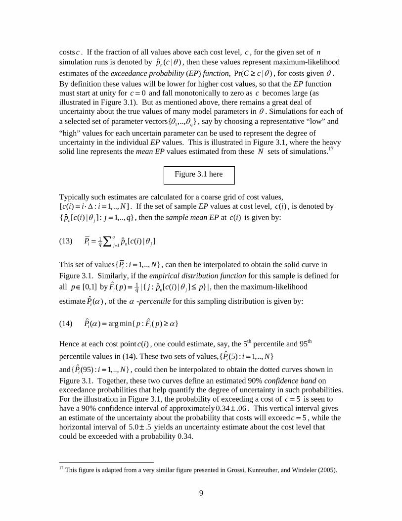
costs c . If the fraction of all values above each cost level, c , for the given set of n simulation runs is denoted by ˆ ( | )np c , then these values represent maximum-likelihood

estimates of the exceedance probability (EP) function, Pr( | )C c , for costs given . By definition these values will be lower for higher cost values, so that the EP function must start at unity for 0c and fall monotonically to zero as c becomes large (as illustrated in Figure 3.1). But as mentioned above, there remains a great deal of uncertainty about the true values of many model parameters in . Simulations for each of a selected set of parameter vectors 1{ ,.., }q , say by choosing a representative “low” and

“high” values for each uncertain parameter can be used to represent the degree of uncertainty in the individual EP values. This is illustrated in Figure 3.1, where the heavy solid line represents the mean EP values estimated from these N sets of simulations.17 Typically such estimates are calculated for a coarse grid of cost values, [ ( ) : 1,.., ]c i i i N . If the set of sample EP values at cost level, ( )c i , is denoted by

ˆ{ [ ( ) | ] : 1,.., }n jp c i j q , then the sample mean EP at ( )c i is given by:

(13) 1

1 ˆ [ ( ) | ]q

i n jjqP p c i

This set of values{ : 1,.., }iP i N , can then be interpolated to obtain the solid curve in

Figure 3.1. Similarly, if the empirical distribution function for this sample is defined for

all [0,1]p by 1ˆ ˆ( ) |{ : [ ( ) | ] } |i n jqF p j p c i p , then the maximum-likelihood

estimate ˆ ( )iP , of the -percentile for this sampling distribution is given by:

(14) ˆ ˆ( ) arg min{ : ( ) }i iP p F p

Hence at each cost point ( )c i , one could estimate, say, the 5th percentile and 95th

percentile values in (14). These two sets of values, ˆ{ (5) : 1,.., }iP i N

and ˆ{ (95) : 1,.., }iP i N , could then be interpolated to obtain the dotted curves shown in

Figure 3.1. Together, these two curves define an estimated 90% confidence band on exceedance probabilities that help quantify the degree of uncertainty in such probabilities. For the illustration in Figure 3.1, the probability of exceeding a cost of 5c is seen to have a 90% confidence interval of approximately 0.34 .06 . This vertical interval gives an estimate of the uncertainty about the probability that costs will exceed 5c , while the horizontal interval of 5.0 .5 yields an uncertainty estimate about the cost level that could be exceeded with a probability 0.34.

17 This figure is adapted from a very similar figure presented in Grossi, Kunreuther, and Windeler (2005).

Figure 3.1 here

10

3.2 Application to the Evaluation of Alternative Earthquake Mitigation Policies Exceedance probability curves provide a useful way to compare loss reduction strategies. In particular, if the cost of a mitigation strategy for Policy denoted by 0C and the

resulting damage costs of shaking and liquefaction are denoted by Sjc and L

jc ,

respectively, then by (3) and (4) above, the net damage costs for Policy can be expressed as:

(15) 01[ (1 ) ]

m L Sj j j j jj

C p c p c C

These comparative costs can readily be estimated within the present probabilistic framework. In Figure 3.2 the estimated curves (plus confidence bands) are plotted for two hypothetical mitigation policies, 1,2 . In this example it turns out that both the mean and variance of damage costs for the distribution corresponding to the mean EP-curve for Policy 2 are lower than those for Policy 1.18 From the viewpoint of standard portfolio analysis, it is tempting to conclude that Policy 2 dominates Policy 1. But it is clear from Figure 3.2 that Policy 2 has a much greater chance of leading to high damage costs than does Policy 1. For example at probability .05 (shown by the dashed horizontal line in the figure) even when uncertainties are taken into account, the chance of damage costs exceeding 8c are less than .05 for Policy 1. However, when taking the uncertainties into account for Policy 2 there is still at least a probability of .05 that damage costs could exceed, 9c . While the above procedure for simulating and estimating both exceedance probabilities and their confidence bands is admittedly very demanding computationally, this methodology appears to yield sharper and more meaningful comparisons of alternative earthquake mitigation policies than those provided by standard portfolio methods. 4. Model Simulation for the Case of Memphis For the present analysis, a contiguous set of 1274n residential parcel sites in Memphis was selected that exhibit a range of liquefaction hazard. The darker red areas in Figure 4.1 show parcel sites with higher levels of liquefaction hazard. For modeling purposes, 7 possible (140 km) rupture events were spaced at about 15 km intervals along each fault line in Figure 2.1. These 21n rupture events are represented

18 These distributions for Policies 1 and 2 are each log normal with respective means and variances given

by 2

1 1( 3.404, .572) and 2

2 1( 3.336, .529) .

Figure 3.2 here

Figure 4.1 here

11

formally by their corresponding earthquake sources (lower ends), as described in Section 2.1. Since the distances between parcel sites are very small compared to distances from these ruptures (as shown in Figure 4.2 below), the closest distance to each rupture event is taken to be the same for all parcels (as represented by the distance to the centroid of these parcel sites). Moreover, most ruptures lie well to the north of the land parcels. The closest point to all parcels for each of these ruptures is simply its corresponding earthquake source, as shown by the 15 earthquake sources in Figure 4.2 (ranging in distance to parcels from about 48 to 120 km). The closest points for the remaining 2 rupture events on each “pseudo fault” line coincide with the lowest earthquake source shown on that fault (which was chosen to be the closest point on the entire fault line). Thus each of these earthquake sources is the closest point for three separate rupture events. In terms of the probability model in expression (2), this implies that the relevant event probability for each of these sites is three times that of its northern neighbors (6/21 versus 2/21 on the central line, and 3/21 versus 1/21 on the outer lines). These probability values are represented by the relative sizes of the dots at each event site in Figure 4.2. For purposes of illustration, we simplify the “logic tree” model in expressions (6) and (9) to a single attenuation function. The earthquake attenuation model of Somerville et al. (2001) was chosen for this analysis.19 Given the above mean distance of 130 km from earthquake sources, this attenuation model predicts sufficiently large mean PGA levels to ensure significant damage within the given set of Memphis parcel sites for a magnitude 7.7 earthquake scenario. The specific parameterization of this model is as follows: for any building site, j, let jr denote the distance from j to the realized earthquake source (as

represented by one of the m sites in Figure 4.1) and set the depth of the rupture event to 0 6h km (following Somerville et al., 2001). The effective distance to the earthquake

source is then given by 2 20( )j jR d r h . For an earthquake of magnitude, M , the mean

log PGA level, j , occurring at site j is taken to be a function of jr and M :

(16) ( , )j j jr M

1 2 0 3 0 4 0( ) ln( ) ( ) ln[ ( )]jM M R M M R r

5 6 0(ln[ ( )] ln[ ( )])j jr R r R r

where (again following Somerville et al., 2001) 1 2 3.239, .805, .679,

4 5 6 0.0861, .00498, .477, 6.4M , and 2 20 0 0 0( )R R d r h with 0 50r .

In all simulations, M is set to 7.7. 19 According to these authors, the basic model form follows that of Abrahamson and Silva (1997).

Figure 4.2 here

12

4.1 Spatial Covariance Model If the vector of mean log PGA values for any given earthquake event is denoted by ( : 1,.., )j j n , then the log PGA levels ( : 1,., )jy y j n generated by this

event are assumed to be multivariate normally distributed as: (17) ( , )y N where the covariance matrix, ( : , 1,.., )ij i j n , allows for possible spatial

dependencies among realized values iy and jy . In the present case, it is postulated that the

covariance, cov( , )ij i jy y , between parcels i and j that are separated by a distance,

ijd , is given by the spherical covariogram in (11). Following Somerville et al. (2001), we

choose the variance 2 .25 , and following Evans (2006), we set the range at 2sr km. A

plot of this covariogram is shown in Figure 2.2. 4.2 Earthquake Destruction Given any realized vector y , of log PGA values, the corresponding vector of PGA values is given by (18) [ exp( ) : 1,.., ]j jA A y j n

To model the damage done by these PGA levels, it is assumed that there is a single threshold level, a , at which structural failure occurs. For purposes of the present analysis, this level was set to 25a (which is by definition 25% of the acceleration of gravity, i.e., / 4g ). Given a lack of data for this Memphis example as to specific damage costs from shaking ( S

jc ) and liquefaction ( Ljc ) at each building site, j , an alternative strategy was adopted.

Here the available data on liquefaction risks at each site is used to modify the likelihood of destruction events. In particular, it is assumed that higher liquefaction risk at site j

translates into a higher effective PGA level, *jA , at j . Specifically, if the liquefaction risk

level at parcel site j (given by “Major Liquefaction Risk” in the Memphis data of Rix

and Romero-Hudock, 2006) is denoted by jLR , then it is assumed that:

(19) * exp( )j j jA A LR

So for example, if a given site j has a liquefaction risk level .12jLR and experiences a

PGA of 23jA , then even though 23 a , this liquefaction risk yields an effective PGA

level,

13

(20) * (23)exp(.12) 25.93 25jA a

A structure at this site is thus more likely to fail than at sites with comparable distances to the rupture event, but with less risk of liquefaction. Finally, given a destruction event at site j , the expected damage cost, jc , is taken to be the building replacement cost from

destruction, as represented by available data on the building value at site j .20 The earthquake simulation was conducted in two stages. In the first stage an earthquake source is simulated using the probability distribution over the 15 earthquake sources in Figure 4.2 (with the specific values mentioned in the discussion of Figure 4.2). Given a simulated draw from this distribution, the distances from the resulting rupture event to each parcel j are calculated and used as the jr values in (16).21 The corresponding mean

vector, , is then calculated, and in the second stage of the simulation, a sample vector of log PGA values, y , is drawn from the multivariate normal distribution in (17) [with mean vector, , and covariance matrix, , given by (10) and (11)]. Hence the

destruction event, j , at parcel site j can then be determined as follows:

(21) *

*

1 ,

0 ,j

jj

A a

A a

Finally, the individual damage costs, jc , based on building values at sites j are used to

determine the total damage cost for the study area due to the earthquake, i.e.,

(22) 1

n

j jjC c

In summary, each simulation run, s , of this two-stage process yields a realized value,

sC , of this random cost variable. By running many simulations, 1,..,s S , a sample

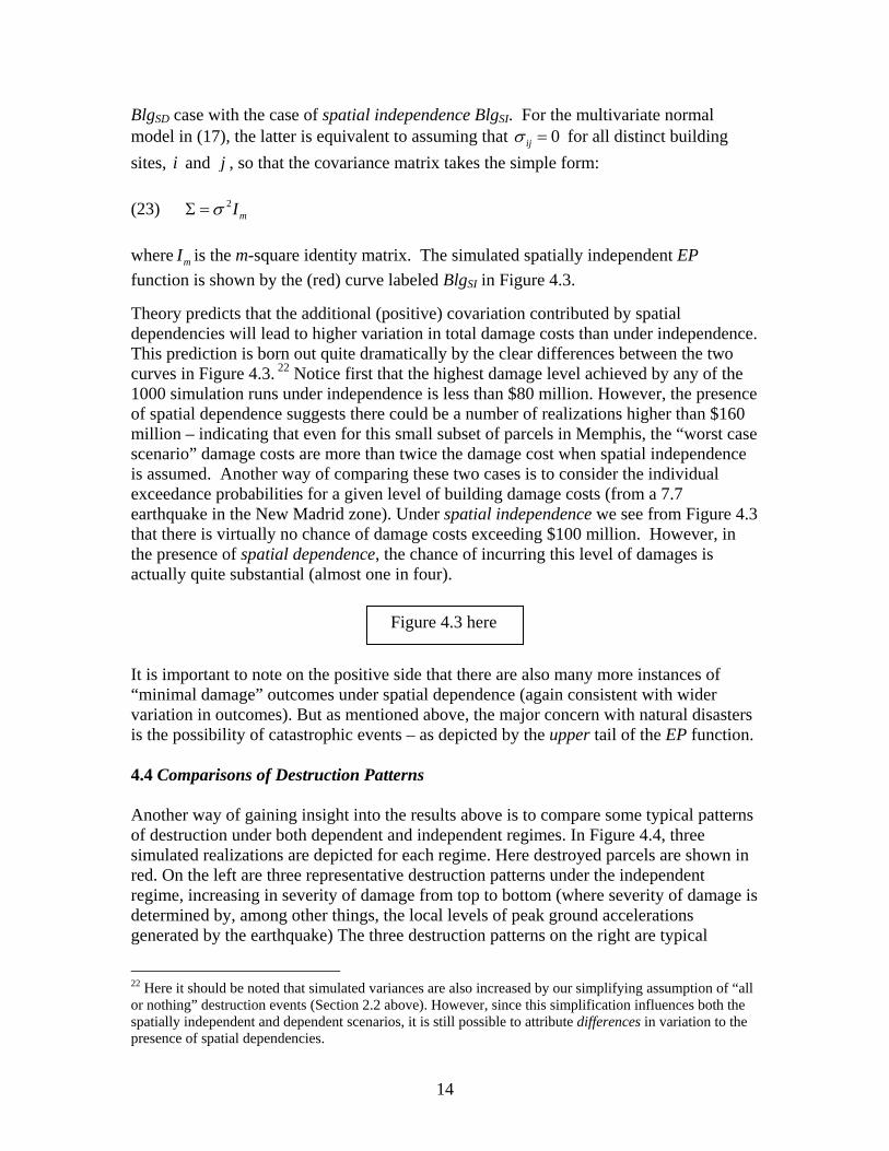
estimate can be obtained for the probability distribution of C . We presume that 1000S is a sufficient number of realizations to obtain a reasonable estimate of this distribution. 4.3 Comparison of Results for Dependent and Independent Destruction Patterns The potential impact of a given natural disaster on a community is most easily studied by plotting the probabilities of exceeding each level of possible damage costs to the community, i.e., the exceedance probability (EP) function. For 1000 simulations, the resulting sample estimate of the EP function for building damage cost under spatial dependence is shown by the (black) curve labeled BlgSD in Figure 4.3. To gauge the effects of spatial dependencies on these probabilities, we compare the spatial dependence

20 All tax roll data and other parcel data for these Memphis sites were obtained from the Shelby County Assessor of Property GIS Department and were dated 2005. 21 Recall that by construction, these 15 earthquake sources turn out to be the closest points from corresponding rupture events to all building sites.

14

BlgSD case with the case of spatial independence BlgSI. For the multivariate normal model in (17), the latter is equivalent to assuming that 0ij for all distinct building

sites, i and j , so that the covariance matrix takes the simple form: (23) 2

mI

where mI is the m-square identity matrix. The simulated spatially independent EP

function is shown by the (red) curve labeled BlgSI in Figure 4.3.

Theory predicts that the additional (positive) covariation contributed by spatial dependencies will lead to higher variation in total damage costs than under independence. This prediction is born out quite dramatically by the clear differences between the two curves in Figure 4.3. 22 Notice first that the highest damage level achieved by any of the 1000 simulation runs under independence is less than $80 million. However, the presence of spatial dependence suggests there could be a number of realizations higher than $160 million – indicating that even for this small subset of parcels in Memphis, the “worst case scenario” damage costs are more than twice the damage cost when spatial independence is assumed. Another way of comparing these two cases is to consider the individual exceedance probabilities for a given level of building damage costs (from a 7.7 earthquake in the New Madrid zone). Under spatial independence we see from Figure 4.3 that there is virtually no chance of damage costs exceeding $100 million. However, in the presence of spatial dependence, the chance of incurring this level of damages is actually quite substantial (almost one in four). It is important to note on the positive side that there are also many more instances of “minimal damage” outcomes under spatial dependence (again consistent with wider variation in outcomes). But as mentioned above, the major concern with natural disasters is the possibility of catastrophic events – as depicted by the upper tail of the EP function. 4.4 Comparisons of Destruction Patterns Another way of gaining insight into the results above is to compare some typical patterns of destruction under both dependent and independent regimes. In Figure 4.4, three simulated realizations are depicted for each regime. Here destroyed parcels are shown in red. On the left are three representative destruction patterns under the independent regime, increasing in severity of damage from top to bottom (where severity of damage is determined by, among other things, the local levels of peak ground accelerations generated by the earthquake) The three destruction patterns on the right are typical

22 Here it should be noted that simulated variances are also increased by our simplifying assumption of “all or nothing” destruction events (Section 2.2 above). However, since this simplification influences both the spatially independent and dependent scenarios, it is still possible to attribute differences in variation to the presence of spatial dependencies.

Figure 4.3 here

15

realizations under the regime of spatial dependence, again increasing in severity from top to bottom. The key difference between these patterns is the more clustered nature of damaged areas in the spatially dependent patterns. [Such clustering consistent, for example, with the liquefaction failure patterns observed for the North Ridge earthquake in southern California (Craven, 1997)]. So if the realized PGA level at a given parcel site is strong enough to cause destruction, then one may infer that the immediate neighbors of this site are quite likely to experience similar outcomes. The exact nature of these destruction patterns will of course depend on many factors, including local geologic conditions and types of building structures. But even without knowledge of all these factors, the simple model of spatial dependencies postulated here is seen to yield simulated patterns of damage that are intuitively more plausible than those under spatial independence. Finally, it is of interest to relate the specific destruction scenarios in Figure 4.4 to the more general EP curves in Figure 4.3. For purposes of illustration, the total building damage costs (Blg) were calculated for high-destruction cases under spatial independence and dependence, as illustrated respectively by scenarios (c) and (f) of Figure 4.4. The total building damage cost for the spatially independent scenario (c) is approximately $63 million (the arrow intersecting the BlgSI curve in Figure 4.3), and the total building damage cost for the spatially dependent scenario (f) is approximately $143 million (the arrow intersecting the BlgSD curve). While these costs involve scenarios that are not directly comparable, it is instructive to observe that the exceedance probabilities for these two scenarios are both about .07. So if independence is assumed, then the BlgSI curve shows that there is about a 7% chance of destruction as extensive as scenario (c). But by allowing for spatial dependence, the BlgSD curve shows that there is about a 7% chance of destruction as extensive as scenario (f), which is more than twice as costly. While these cost comparisons involve only a single level of spatial dependence, and do not account for any additional model uncertainties, they serve to illustrate the potentially dramatic difference in risk assessments between the two cases. 4.5 A Policy Example Hazards policies, regulations, and standards are implemented as a collective or societal choice. The following example illustrates a hypothetical decision for a community that is considering the adoption of a mitigation plan for a future earthquake hazard. The objective of this example is to show that failure to account for unobserved spatial dependencies can lead to an underestimation of potential damages, causing decision makers to believe they are better off than they actually are. Underestimation of future damage costs could lead to an under-investment in mitigation resulting in even greater damages and slower recovery (such as the recovery following Hurricane Katrina; Vigdor, 2008, Masozura, 2008).

Figure 4.4 here

16

Here we assume that for the Memphis neighborhood in Figure 4.2, the relevant exceedance probability curves are those shown as red in Figure 4.5. However, it should be noted that a 7.7 earthquake scenario is not sufficiently comprehensive for analysis of loss reduction strategies. Thus we view the following analysis as representative of a range of earthquake scenarios that would need to be considered. Furthermore, we also have ignored the bands of model-added uncertainty in Figures 3.1 and 3.2. To apply these EP curves in the present example, we assume that risk assessment for this earthquake mitigation decision is carried out in terms of Value-at-Risk estimation.23 This approach begins by identifying a relevant investment time frame, T , together with a relevant risk level, , and then seeks to estimate the minimum loss level, ( , )L L T , that will be exceeded with probability in time period T . This loss, L , is then referred to as the value at risk (VaR) for the investment relative to andT . It is appropriate to adopt a time frame of 50T years, as a “building lifetime” benchmark used by standard building codes.24 For ease of illustration, it is convenient to choose a risk level of .005 , i.e., of “five-in-a-thousand”. Hence the relevant VaR from earthquakes is taken to be the minimum level L , for which there is only a five-in-a-thousand chance of incurring losses as large as L within the next 50 years. Our example supposes that the given mitigation plan involves both private and public investments for Memphis. Although the mitigation plan would cover the entire Memphis area, we apply the plan to the neighborhood in Figure 4.2 and assume that the total investment cost for this neighborhood would be $15 million. Further we assume that this plan will only be worthwhile if the value at risk (VaR) is a least ten times this amount, i.e., at least $150 million. To calculate VaR we combine the conditional exceedance probabilities (Figure 4.5) based on the occurrence of a 7.7 earthquake with the occurrence probability of a 7.7 earthquake to determine the unconditional exceedance probabilities. While there is a great deal of uncertainty in the estimation of such probabilities, Frankel (2004) has estimated that based on an observed average recurrence time of 500 years, the chance of a 7.7 earthquake occurring in the New Madrid zone within the next 50 years is 10%. The unconditional exceedance probability corresponding to a risk level of .005 is thus obtained by dividing by .10 to yield: (24) / .10 .005/.10 .05EP

23 Value-at-Risk estimation is a common tool for analysis of financial risk. This methodology is detailed for example in Duffy, Manfredo and Leuthold (1999), Duffie and Pan (1997), and Ridder (1998). 24 Of course this ignores the fact that many existing building may have shorter lifetimes.

Figure 4.5 here

17

The horizontal dashed line at .05EP in Figure 4.5 identifies the relevant VaR on each curve. Here it is seen that under spatial independence, the relevant value at risk is somewhere in the interval of values between points a and b in Figure 4.5, which range from about $65 million to $85 million. It can be argued by opponents of this policy that the relevant VaR is most likely less than $150 million, and that in view of the costs of these investments, such a mitigation plan would not be worthwhile. However, in the presence of spatial dependencies, the relevant interval of values at risk is given by point c and point d in Figure 4.5, which range from about $150 million to $200 million. Therefore when spatial dependencies are taken into account, the relevant value at risk is seen to be much larger, and is indeed quite likely to exceed $150 million. Thus in the present case this factor alone might convince decision makers that the proposed mitigation plan is well worth the cost. There is an important additional dimension of uncertainty that is shown in Figure 4.5. While building values reflect the costs of replacing structures destroyed by the earthquake, there are in fact many additional costs resulting from amenity damage external to individual building sites (as discussed in the Appendix). Replacement costs may in fact represent a lower bound of total costs. Though it is difficult to estimate the full extent of costs due to loss of amenities (discussed further in the Appendix), it can be argued that their ultimate effect will be to depress local land values as represented by a long term decline in property values (e g., Hurricane Katrina). Depending on the scale of damage, planning time horizon, and existing regulations, the total value (Tot) of site (Building value + Land value25) may be taken as a reasonable upper bound on total economic losses at each site. These values also have been obtained for Memphis (see footnote 13) and have been used to construct the augmented EP curves, TotSI and TotSD, shown in Figure 4.5. For example, the horizontal displacement between the two curves BlgSI and TotSI represent the total land value of all sites destroyed at each level of exceedance probability under the spatial independence scenario. These horizontal intervals can be interpreted as bounding the potential damage costs at each level of exceedance probability. Of course it is rarely the case that any single consideration will be decisive in such a complex policy question. The main point of this example is to show that the possibility of spatial dependencies in earthquake outcomes constitutes one important factor that must be considered in the proper assessment of earthquake risks. 5. Concluding Remarks While the proposed procedure for simulating and estimating both exceedance probabilities and their confidence bands is admittedly very demanding computationally, this methodology yields a flexible and effective approach for the comparison of alternative hazard mitigation plans. Our simulation results suggest that this model does indeed provide a framework within which the risk of catastrophic earthquake events can be analyzed. In particular, it highlights the potential importance of incorporating spatial dependencies into such models. 25 Here Land value is taken to reflect both site and community amenities.

18

However, there are a number of caveats that should be mentioned. First, we have made a number of simplifying assumptions in the above model, such as the assumption of all-or-nothing damage outcomes, rather than more realistic (but elaborate) fragility curves. Also, in the empirical example analyzed, we have considered only a small portion of the Memphis area (again for computational simplicity). Moreover, we have chosen to consider only a set of contiguous parcels. While parcel contiguity allows a more meaningful visual representation of destruction patterns (such as those in Figure 4.4), it is important to emphasize that such contiguity also tends to dramatize the effects of spatial dependencies. In particular, since all between-parcel distances in the present study area are within the dependency range of 2 km, each parcel pair exhibits some degree of spatial dependency. Hence it should be clear that local dependency effects are more dramatic than they would be if the entire Memphis area were included (where many parcel pairs are independent). But regardless of how large the study area may be, it is also clear that if spatial dependencies are ignored then the true likelihood of catastrophic outcomes will surely be underestimated. Finally it should be emphasized that while our simple policy example in section 4.5 illustrates a possible application of this modeling framework to policy analysis, more realistic policy analyses typically involve the comparison of many alternatives. Moreover, as discussed in section 3.2, a more meaningful comparison of such policies must involve not only the cost uncertainties illustrated in section 4.5, it also should include a range of model-added uncertainties, as illustrated in Figure 3.2. Hence one important direction for extending the present modeling and simulation framework is to incorporate the full range of such uncertainties in a systematic way. Thus the work reported here is best viewed as an initial effort to integrate scientific information, hazard event uncertainty, and model uncertainty to inform decision making about natural disasters at the regional scale. Acknowledgements The authors would like to thank Joan Gomberg and Cynthia Wallace for their instructive reviews. References Abrahamson, N., and W. Silva, 1997, Empirical response spectral attenuation relations for shallow crustal earthquakes, Seismological Research Letters, v. 68, p.94-127. Boore, D.. 1997, Estimates of average spectral amplitudes at FOAKE sites, Appendix C in An Evaluation of Methodology for Seismic Qualification of Equipment, Cable Trays, and Ducts in ALWR Plants by use of Experience Data,

19

K. Bandyopadhyay, D. Kana, R. Kennedy, and A. Schiff,(ed., U.S.?? Nuclear Regulatory Commission NUREG/CR-6464 and Brookhaven National Lab BNL-NUREG-52500, C-1-C-69. Boore, D., J. Gibbs, W. Joyner, J. Tinsley, and D. Ponti, 2003, Estimated ground motion from the 1994 Northridge, California earthquake at the site of the Interstate 10 and La Cienega Boulevard Bridge collapse, West Los Angeles, California, Bulletin of the Seismological Society of America, v. 93, p.2737-2751. Chang, S., W. Svelka, and M. Shinozuka, 2002, Linking infrastructure and urban economy: simulation of water-disruption impacts in earthquakes, Environment and Planning B, 29:281-301. Cramer, C., 2001, A seismic hazard uncertainty analysis for the New Madrid Seismic Zone, Engineering Geology, v. 62, p.251-266. Craven, A., 1997, The Quantitative Estimation of Earthquake-Induced Ground Failure in the San Fernando Valley, California, Thesis manuscript, Stanford University, 74p., 8 plates. Duffy, D., and J. Pan, 1997, A Overview of Value at Risk, preliminary draft, 39p. Elnashai, A., L. Cleveland, T. Jefferson, and J. Harrald, 2008, Impact of Earthquakes on the Central USA, Mid-America Earthquake Center Report 08-02, Mid-America Earthquake Center, Urbana, Illinois, https://www.ideals.uiuc.edu/handle/2142/8971, 936p. Evans, John (2006). Personal Communication. FEMA (2003). HAZUS-MH MR-1 Technical Manual. Federal Emergency Management Agency, Washington, D.C. Frankel, A., C. Mueller, T. Barnhard, D. Perkins, E. Leyendecker, N. Dickman, S. Hanson, and M. Hopper, 1996, National seismic hazard maps: Documentation June, 1966, Open-File Report 97-131, US Geological Survey, ?p. Frankel, A., C. Mueller, T. Barnhard, D. Perkins, E.V. Leyendecker, N. Dickman, S. Hanson, and M. Hopper, 2002, Documentation for the 2002 of the national seismic hazard maps, Open-File Report 97-131, US Geological Survey. Frankel, A., 2005, Personal Communication. Goda, K. and H. Hong, 2008, Spatial correlation of peak ground motions and response spectra, Bulletin of the Seismological Society of America, v. 98, p.354-365. Goodno, B., A. Bostrom, J. Craig, and J. Park, 2006, Probabilistic Decision Support for

20

Regional Risk Assessment, Final Report, Georgia Institute of Technology, Atlanta,GA, http://smartech.gatech.edu/dspace/handle/1853/23037, 235p. Gordon, P., J. Moore, II, H. Richardson, M. Shinozuka, D. An, and S. Cho, 2004, Earthquake disaster mitigation for urban transportation systems: an integrated methodology that builds on the Kobe and Northridge experiences, in Modeling Spatial and Economic Impact of Disasters, Chang, S., and Y. Okuyama, eds., Springer: New York, 323p. Grossi, P., H. Kunreuther, and D. Windeler, 2005, An introduction to catastrophe models and insurance, in Grossi, P. and H. Kunreuther, eds., Catastrophe modeling: a new approach to managing risk, Springer: New York, 245p. Karaca, E. and Luco, N, 2006. Probabilistic Seismic Loss Analysis for Bridges in the Central United States, Proceedings of the 5th National Seismic Conference on Bridges and Highways, September 18-20, 2006 Major, J., 1999, Index hedge performance: insurer market penetration and basis risk, in Froot, K., ed., The Financing of Catastrophe Risk, University of Chicago Press, 463p. Manfredo, M., and R. Leuthold, 1999, Value-at-Risk Analysis: A Review and the Potential for Agricultural Applications, Review of Agricultural Economics, v. 21, p.99-111. National Institute of Building Safety, 1997, HAZUS: Hazards U.S.: Earthquake loss estimation methodology, NIBS Document Number 5200, National Institute of Building Sciences, Washington, DC. Ridder, T., 1998, Basics of statistical VaR-Estimation, in Bol, G., G. Nakhaeizadeh, and K-H. Vollmer, eds., Risk Measurement, Econometrics and Neural Networks, Physica-Verlag, Heidelberg, 306p. Rix, G.J. and S. Romero-Hudock, 2006, Liquefaction Potential Mapping in Memphis and Shelby County, Tennessee, USGS Report, available at the web site:http://earthquake.usgs.gov/regional/ceus/products/liq_download.php. Schabenberger, O. and C.A. Gotway, 2005, Statistical Methods for Spatial Data Analysis, Chapman-Hall/CRC: New York, ?p. Shinozuka, M., and S. Chang, 2004, Evaluating the Disaster resilience of Power Networks and Grids, in Okuyama, Y., and S. Chang (eds.), Modeling Spatial and Economic Impacts of Disasters, Springer, Berlin, 323p. Sinn, H-W, 1983, Economic decisions under uncertainty, North-Holland, Amsterdam, 359p.

21

Somerville, P., N. Collins, N. Abrahamson, R. Graves, and C. Saika, 2001, Ground motion attenuation relations for the Central and Eastern United States, USGS Report, Award 99HQGR0098. Stover, C., and J. Coffman (1993), Seismicity of the United States, 1568-1989, (revised), USGS Professional Paper 1527, USGS, Denver, 418p. United States Geological Survey, 1996, USGS Response to an urban Earthquake: Northridge ’94, USGS Open-File Report 96-263, USGS, Denver, 78p. Wang, M. and T. Takada, 2005, Macrospatial correlation model of seismic ground motions, Earthquake Spectra, 21: 1137-1156. Wells, D., and K. Coppersmith. 1994, New empirical relations among magnitude, rupture length, rupture width, rupture area, and surface displacement, Bulletin of the Seismological Society of America, 84: 974-1002. Wesson, R., and D.Perkins, 2001, Spatial correlation of probabilistic earthquake ground motion and loss, Bulletin of the Seismological Society of America, 91: 1498-1515.

Wesson, R. L., Perkins, D. M., Luco, N., & Karaca, E. (2009). Direct calculation of the probability distribution for earthquake losses to a portfolio. Earthquake Spectra, 25(3), 687-706.

22

APPENDIX: Model Extensions to Include Losses External to Individual Sites NOT READ

The model developed in this paper focuses only on damage costs, jc , that are directly

attributable to individual sites, jb . But it is clear that such sites do not exist in isolation.

Here we briefly consider two possible extensions of the present model to incorporate losses incurred at sites jb resulting from destruction occurring elsewhere in space. First

we consider losses due to destruction of other sites in the area, and then consider losses due to the destruction of more global types of amenities or infrastructure. Recall that some degree of spatial interdependency between sites was introduced by allowing spatial autocorrelation among realized PGA levels. More importantly, by focusing on the joint realization ( : 1,.., )jA A j m , of PGA levels at all sites, it is

possible to use this joint framework to incorporate losses due to the simultaneous destruction of whole neighborhoods. For example, if site jb is located within an historic

neighborhood that adds value to this site, then destruction of this entire neighborhood creates additional loss of value at jb beyond that resulting from on-site structural damage.

As a second example, suppose that site jb is located in a school district with an

elementary school at site s . Then the destruction of buildings at site s must result in some loss of value at jb .26 These values can be estimated as part of a hedonic regression (an

econometric model for property valuation) that includes such neighborhood amenities. In particular, if jN denotes the family of relevant amenity neighborhoods (site ensembles),

jN , for site jb with respect to specific amenities, and if the hedonic value of amenity

neighborhood jN , to site jb is denoted by ( )j jc N , then this value constitutes the loss

incurred at jb from the joint destruction of all sites in jN .

Here the definition of an “amenity neighborhood” is meant to be broad in scope. In the historic-area example above, if destruction occurs only in part of this area (possibly not including site jb ) then there is still some loss incurred at jb . Hence in this case, the

definition of jN should include a sufficient number of representative site ensembles, jN ,

in this area to reflect an appropriate range of “degrees of destruction” to the area as a whole. Note also in the school example above that the relevant site ensemble { }jN s ,

need not include site jb as a member. With this broad definition, if we now let the

destruction event for each amenity neighborhood jN , be denoted by the joint event,

26 While schools (unlike historic sites) can be rebuilt, such reconstruction takes time as well as money.

Hence destruction of schools should reduce the present resale value of sites j

b as family residences.

23

(A.1) j j

N hh N

(so that 1 1jN h for all jh N ), then the total damage cost in expression (3) of

the text can now be extended to a function of the form

(A.3) 1

( )jj j

m

j j N j jj NC c c N

N

The key point here is that if all relevant neighborhood sites are already included in{1,.., }m , then exactly the same probability framework above can be applied to this more general cost model. On the other hand, if some sites are not included in{1,.., }m , then the relevant PGA vector A , must now be extended to include these sites, say

( : ) ,Q jA A j Q where

(A.4) 1{ }

Nj j

m

j jj NQ b N

and relation (5) in the text must be extended to include the additional conditions that

(A.5) ( ) 1 ,j h h jN A a h N

for all , 1,..,j jN j mN . The total damage costsC , are determined by the joint

distribution of PGA levels, and hence can be analyzed within our present framework.

In addition to site-based amenities, there are many important types of urban amenities and infrastructure that are not considered sites themselves, but nonetheless influence the overall value of sites jb . For example, a well known urban hazard arising from

earthquakes is the possibility of widespread fires. Fires can potentially destroy public amenities, such as park areas and tree-lined streets that may not be directly affected by ground motion. Another possibility is the destruction of transportation networks or water supply networks that are spread over space and hence not site specific.27 While there is a high degree of uncertainty as to the both the location and extent of such events, it seems reasonable to hypothesize that all earthquake-related information needed for the prediction and evaluation of each such event is contained in the joint spatial realization of PGA levels. More formally, if we now let H denote the relevant set of public hazard events h , (such as destruction of a given park or bridge) and let h denote the indicator

variable for event, h H , then by extending sitesQ , in (A.4) to a larger set HQ ,

including those sites where ground motion might contribute to the occurrence of some hazard event h H , it is here postulated that all earthquake information for the event occurrence, 1h , is contained in the joint PGA realization ( : )H j HA j QA , i.e., that

for all h H ,

(A.6) Pr( 1| , , ) Pr( 1| )h H i h Hx MA A

27 For disaster analyses of this type, see for example Chang et al. (2002) and Gordon et al. (2004).

24

If ( )jc h denoted the value contributed to site jb by the presence of the hth amenity, and if

we again take this value to constitute the loss at jb resulting from destruction

event, 1h , then the total cost model in (A.3) can be further extended to

(A.7) 1

( ) ( )N jj j

m

j j N j j h jj N h HC c c N c h

In this context, expression (9) in the text together with (A.6) provides a well-defined distribution theory for the analysis of total cost realizations in (A.7).

25

Memphis

Figure 2.1: New Madrid Zone Relative to Memphis (Legend: line of recent microearthquake activity, outside boundary for Realfoot Rift, circles denote earthquakes of magnitude at least 3.0 since 1976) EXPLAIN BLACK DOTS?

0 0.5 1 1.5 2 2.50

0.05

0.1

0.15

0.2

0.25

Figure 2.2: A Spherical Covariogram: 2 .25 , and 2sr km.

sr

cov ( )s d

d

26

0 1 2 3 4 5 6 7 8 9 100

0.1

0.2

0.3

0.4

0.5

0.6

0.7

0.8

0.9

1

c

( )P c

Cost Uncertainty

Probability Uncertainty

95-percentile

5-percentile

Mean Exceedance Probabilities

Figure 3.1: Exceedance Probability Curves

0 1 2 3 4 5 6 7 8 9 100

0.1

0.2

0.3

0.4

0.5

0.6

0.7

0.8

0.9

1

Policy 1

Policy 2

EP

Figure 3.2. Comparison of Two Mitigation Policies

27

Figure 4.2: Earthquake Sources

!

!

!

!

!

!

!

!

!

!

!

!

!

!

!

Earthquake Sources

Parcel Sites

Figure 4.1: Parcel Sites in Memphis

28

0 20 40 60 80 100 120 140 160 1800

0.1

0.2

0.3

0.4

0.5

0.6

0.7

0.8

0.9

1

Figure 4.3: Comparison of EP Functions for Building Damage Costs ($Millions)

BlgSI BlgSD

EP

0.24

29

Figure 4.4: Comparison of Typical Destruction Patterns (red = destroyed; yellow = not destroyed)

a

b

c

d

e

f

30

0 50 100 150 200 2500

0.1

0.2

0.3

0.4

0.5

0.6

0.7

0.8

0.9

1

EP

BlgSI

BlgSD

TotSI

TotSD

a 0.05

b c d

Figure 4.5: Comparison of EP curves for Building and Total Damage Costs ($Millions) for both the Spatially Independent and Dependent Models