A State Distillation Protocol to Implement Arbitrary Single-qubit Rotations

Guillaume Duclos-Cianci1, ∗ and Krysta M. Svore2, †

1Department de Physique, Universite de Sherbrooke, Sherbrooke, Quebec, J1K 2R1 (Canada)2Quantum Architectures and Computation Group,Microsoft Research, Redmond, WA 98052 (USA)

(Dated: October 9, 2012)

An important task required to build a scalable, fault-tolerant quantum computer is to efficientlyrepresent an arbitrary single-qubit rotation by fault-tolerant quantum operations. Traditionally,the method for decomposing a single-qubit unitary into a discrete set of gates is Solovay-Kitaevdecomposition, which in practice produces a sequence of depth O(logc(1/ε)), where c ∼ 3.97 is thestate-of-the-art. The proven lower bound is c = 1, however an efficient algorithm that saturatesthis bound is unknown. In this paper, we present an alternative to Solovay-Kitaev decompositionemploying state distillation techniques which reduces c to between 1.12 and 2.27, depending onthe setting. For a given single-qubit rotation, our protocol significantly lowers the length of theapproximating sequence and the number of required resource states (ancillary qubits). In addition,our protocol is robust to noise in the resource states.

PACS numbers: 03.67.Lx, 03.67.Pp, 03.65.FdKeywords: state distillation, Solovay-Kitaev decomposition

Given recent progress in quantum algorithms, quan-tum error correction, and quantum hardware, a scalablequantum computer is becoming closer and closer to re-ality. For many proposed quantum computer architec-tures, e.g., topological systems based on the braiding ofnon-Abelian anyons [1–5] or the surface code model basedon code deformation [6, 7], so-called Clifford operationsand stabilizer state preparations or measurements can beimplemented efficiently and accurately. However, theseoperations alone are not sufficient for quantum univer-sality since they can be simulated classically [8–10]. Onetechnique to achieve quantum universality is to use magicstate distillation [11–13] to augment the set with a singlenon-Clifford operation, e.g., the single-qubit π/8 gate,T . This augmented set can be used to approximate anysingle-qubit unitary using Solovay-Kitaev decomposition[14].

The Solovay-Kitaev theorem [15] states that for any εand single-qubit gate U , U can be approximated to pre-cision ε using Θ(logc(1/ε)) gates drawn from a universal,discrete gate set, where c is a small constant. State-of-the-art implementations of Solovay-Kitaev decompo-sition result in c ∼ 3.97 [14, 16], resulting in an averagedecomposition sequence with hundreds to thousands ofT gates [16]. Each T gate requires a number of copies ofa quantum magic state |H〉 (Hadamard +1-eigenstate),where the number depends on the specific state distilla-tion protocol and purity of the state [11–13]. Therefore,it is especially important to minimize the number of Tgates when decomposing a rotation, since each T gaterequires additional ancillary qubits for implementation.

In this paper, we present an alternative protocol toSolovay-Kitaev decomposition that allows the implemen-

∗ Guillaume.Duclos-Cianci@USherbrooke.ca† ksvore@microsoft.com

tation of single-qubit rotations through the use of dis-tilled magic |H〉 states. We show that the resources re-quired by our protocol are substantially fewer than theresources required by state-of-the-art implementations ofSolovay-Kitaev decomposition [16], in both the numberof gates and the number of quantum magic states neces-sary to apply an arbitrary single-qubit unitary.

I. MAGIC STATE DISTILLATION ANDIMPLEMENTATION OF ROTATIONS

Solovay-Kitaev decomposition [14–16] enables the ap-proximation of any gate using an approximately universalset of elementary gates, e.g., {H,T,Λ(X)}, where Λ(X)denotes the controlled-NOT gate. In particular, one canapproximate any single-qubit unitary operation using theset {H,T}. Magic state distillation is then used to pro-duce the magic |H〉 states necessary to implement the Tgate.

We call a state |ψ〉 magic if given n noisy copies of |ψ〉and the ability to perform perfect Clifford operations, wecan obtain, or “distill”, a purer copy of |ψ〉 from a Cliffordcircuit applied to the n noisy copies of |ψ〉. We can thenobtain even purer states which are arbitrarily close tothe perfect state by applying the protocol recursively [11–13]. These distilled states can be used to implement non-Clifford operations, e.g., the T gate, as described below.

We briefly review how to perform an arbitrary rotationabout the Z-axis using a resource state, and how to ap-ply the T gate. We assume that Clifford operations areapplied perfectly, since they can be implemented fault-tolerantly, and that the resource states are very close topure. One can use the protocols of [11, 12] to performthe initial distillation in order to obtain arbitrarily pureresource states for input. We focus on the +1 eigenstate

arX

iv:1

210.

1980

v1 [

quan

t-ph

] 6

Oct

201

2

2

|Z(θ)〉 X(Z) |m〉

|ψ〉 • Z(X)(−1mθ) |ψ〉

FIG. 1. Circuit randomly implementing a rotation of angle±θ around the Z(X)-axis.

of the Hadamard operation, H,

|H〉 = cosπ

8|0〉+ sin

π

8|1〉 ,

and omit the cost of the initial distillation of the |H〉state. We concentrate on single-qubit states found in ei-ther the XZ- or XY -plane of the Bloch sphere. Note thatone can easily move a state from one plane to the otherby the application of the Clifford HSHX operation.

Suppose we start with states |Z(θ)〉 and |ψ〉:

|Z(θ)〉 = |0〉+ eiθ |1〉 ,|ψ〉 = a |0〉+ b |1〉 .

The circuit to implement a rotation around the Z-axis,presented in Fig. 1, leads to the two-qubit state

|Z(θ)〉 |ψ〉 = a |00〉+ b |01〉+ aeiθ |10〉+ beiθ |11〉Λ(X)−−−→ a |00〉+ b |11〉+ aeiθ |10〉+ beiθ |01〉 .

Upon measurement of the first qubit in the computa-tional basis, we obtain

m=0−−−→ a |0〉+ beiθ |1〉 ,m=1−−−→ aeiθ |0〉+ b |1〉 = a |0〉+ be−iθ |1〉 ,

each with probability 1/2. Thus, the angle of rotation ischosen at random to be θ or −θ, up to global phase. Ananalogous circuit performs a rotation about the X-axis.Similar circuits can be found in [7].

As an important example of this procedure, considerthe XY -plane version of the |H〉 state:

|Z(π/4)〉 = HSHX |H〉 = |0〉+ eiπ/4 |1〉 .

Using the circuit in Figure 1, we can implement a Z-rotation of angle ±π/4, producing at random either theT gate or its adjoint, T †. In this particular case, wecan deterministically apply the desired gate T or T † byapplying the phase gate S, since ST † = T . In general,however, this deterministic correction will not be possi-ble.

II. NEW STATES FROM |H〉 STATES

In this section, we show that we can use a very simpletwo-qubit Clifford circuit to obtain other non-stabilizerstates using only |H〉 states as an initial resource, andthen show that these states enable the approximation of

|H0〉 X |0〉 (|1〉)

|Hi〉 • |Hi+1〉 (|Hi−1〉)

FIG. 2. Two-qubit circuit used to obtain new |Hi〉 states frominitial resource states |H0〉. Upon measuring the 0 outcome,the output state is |Hi+1〉. Upon measuring the 1 outcome,the output state is |Hi−1〉.

any single-qubit rotation. We assume that we are pro-vided with perfect copies of |H〉. We would like to mini-mize the number of |H〉 states required to implement anarbitrary single-qubit rotation, since these distilled statescan be costly to produce.

Consider the circuit of Fig. 2. One can easily verifythat it measures the parity of the two input qubits anddecodes the resulting state into the second qubit. Webegin by considering the two inputs to be |H〉 states. Wedefine θ0 = π

8 and |H〉 = |H0〉 = cos θ0 |0〉 + sin θ0 |1〉.The circuit begins as:

|H0〉 |H0〉 = cos2 θ0 |00〉+ sin2 θ0 |11〉+ cos θ0 sin θ0(|01〉+ |10〉)

Λ(X)−−−→ cos2 θ0 |00〉+ sin2 θ0 |01〉+ cos θ0 sin θ0(|11〉+ |10〉).

Upon measurement of the first qubit, we have

m=0−−−→ cos2 θ0 |0〉+ sin2 θ0 |1〉cos4 θ0 + sin4 θ0

,

m=1−−−→ 1√2

(|0〉+ |1〉).

We define θ1 such that

cos θ1 |0〉+ sin θ1 |1〉 =cos θ0 |0〉+ sin θ0 |1〉

cos4 θ0 + sin4 θ0

,

from which we deduce cot θ1 = cot2 θ0. We define |H1〉 =cos θ1 |0〉+ sin θ1 |1〉, a non-stabilizer state obtained from|H〉 states, Clifford operations, and measurements. Ifthe outcome of the measurement is 1, then we obtain astabilizer state and discard the output (see Fig. 2).

The two measurement outcomes occur with respectiveprobabilities

p0 = cos4 θ0 + sin4 θ0 =3

4,

p1 = 1− p0 =1

4.

We now recurse on this protocol using the non-stabilizer states produced by the previous round of theprotocol as part of the input to the circuit of Fig. 2. Wedefine

|Hi〉 = cos θi |0〉+ sin θi |1〉 ,cot θi = coti+1 θ0.

3

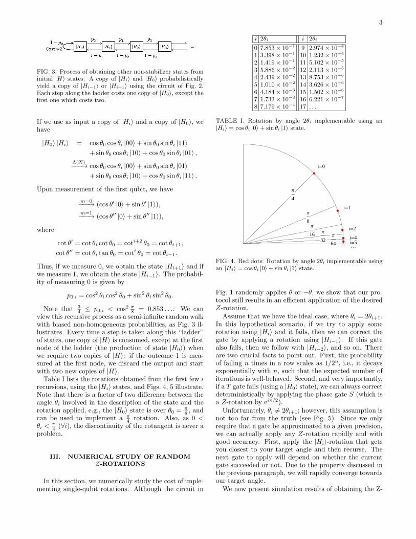
FIG. 3. Process of obtaining other non-stabilizer states frominitial |H〉 states. A copy of |Hi〉 and |H0〉 probabilisticallyyield a copy of |Hi−1〉 or |Hi+1〉 using the circuit of Fig. 2.Each step along the ladder costs one copy of |H0〉, except thefirst one which costs two.

If we use as input a copy of |Hi〉 and a copy of |H0〉, wehave

|H0〉 |Hi〉 = cos θ0 cos θi |00〉+ sin θ0 sin θi |11〉+ sin θ0 cos θi |10〉+ cos θ0 sin θi |01〉 ,

Λ(X)−−−→ cos θ0 cos θi |00〉+ sin θ0 sin θi |01〉+ sin θ0 cos θi |10〉+ cos θ0 sin θi |11〉 .

Upon measurement of the first qubit, we have

m=0−−−→ (cos θ′ |0〉+ sin θ′ |1〉),m=1−−−→ (cos θ′′ |0〉+ sin θ′′ |1〉),

where

cot θ′ = cot θi cot θ0 = coti+2 θ0 = cot θi+1,

cot θ′′ = cot θi tan θ0 = coti θ0 = cot θi−1.

Thus, if we measure 0, we obtain the state |Hi+1〉 and ifwe measure 1, we obtain the state |Hi−1〉. The probabil-ity of measuring 0 is given by

p0,i = cos2 θi cos2 θ0 + sin2 θi sin2 θ0.

Note that 34 ≤ p0,i < cos2 π

8 = 0.853 . . .. We canview this recursive process as a semi-infinite random walkwith biased non-homogeneous probabilities, as Fig. 3 il-lustrates. Every time a step is taken along this “ladder”of states, one copy of |H〉 is consumed, except at the firstnode of the ladder (the production of state |H0〉) whenwe require two copies of |H〉: if the outcome 1 is mea-sured at the first node, we discard the output and startwith two new copies of |H〉.

Table I lists the rotations obtained from the first few irecursions, using the |Hi〉 states, and Figs. 4, 5 illustrate.Note that there is a factor of two difference between theangle θi involved in the description of the state and therotation applied, e.g., the |H0〉 state is over θ0 = π

8 , andcan be used to implement a π

4 rotation. Also, as 0 <θi <

π4 (∀i), the discontinuity of the cotangent is never a

problem.

III. NUMERICAL STUDY OF RANDOMZ-ROTATIONS

In this section, we numerically study the cost of imple-menting single-qubit rotations. Although the circuit in

i 2θi i 2θi

0 7.853× 10−1 9 2.974× 10−4

1 3.398× 10−1 10 1.232× 10−4

2 1.419× 10−1 11 5.102× 10−5

3 5.886× 10−2 12 2.113× 10−5

4 2.439× 10−2 13 8.753× 10−6

5 1.010× 10−2 14 3.626× 10−6

6 4.184× 10−3 15 1.502× 10−6

7 1.733× 10−3 16 6.221× 10−7

8 7.179× 10−4 17 . . .

TABLE I. Rotation by angle 2θi implementable using an|Hi〉 = cos θi |0〉+ sin θi |1〉 state.

Π

4

Π

8Π

16 Π

32Π

64

i=0

i=1

i=2

i=4i=5…

FIG. 4. Red dots: Rotation by angle 2θi implementable usingan |Hi〉 = cos θi |0〉+ sin θi |1〉 state.

Fig. 1 randomly applies θ or −θ, we show that our pro-tocol still results in an efficient application of the desiredZ-rotation.

Assume that we have the ideal case, where θi = 2θi+1.In this hypothetical scenario, if we try to apply somerotation using |Hi〉 and it fails, then we can correct thegate by applying a rotation using |Hi−1〉. If this gatealso fails, then we follow with |Hi−2〉, and so on. Thereare two crucial facts to point out. First, the probabilityof failing n times in a row scales as 1/2n, i.e., it decaysexponentially with n, such that the expected number ofiterations is well-behaved. Second, and very importantly,if a T gate fails (using a |H0〉 state), we can always correctdeterministically by applying the phase gate S (which isa Z-rotation by eiπ/2).

Unfortunately, θi 6= 2θi+1; however, this assumption isnot too far from the truth (see Fig. 5). Since we onlyrequire that a gate be approximated to a given precision,we can actually apply any Z-rotation rapidly and withgood accuracy. First, apply the |Hi〉-rotation that getsyou closest to your target angle and then recurse. Thenext gate to apply will depend on whether the currentgate succeeded or not. Due to the property discussed inthe previous paragraph, we will rapidly converge towardsour target angle.

We now present simulation results of obtaining the Z-

4

10 20 30 40i

10-12

10-9

10-6

0.001

1Θ

FIG. 5. Dots: States obtainable by recursively using the cir-cuit of Fig. 2 and only |H〉 states as initial input. Full line:exponential decay fit, θi ∼ 2.41−0.881i.

rotation Z(φ), where φ is chosen randomly, in order tocharacterize the efficiency of the protocol proposed inprevious sections. The simulation proceeds as follows:

1. Set desired accuracy ε.

2. Randomly pick a target rotation angle 0 < φ < 2π.

3. Find the state |Hi〉 such that 2θi is close to φ.

4. Simulate an instance of the ladder to obtain thatstate and add its cost to the offline cost.

5. Apply a rotation using the |Hi〉 state and the circuitof Fig. 1 and add one to the online cost.

6. Recurse on steps 3 through 5 until the desired ac-curacy is reached.

We define the accuracy of the applied rotation V com-pared to the target rotation U as

max|ψ〉

D(U |ψ〉 〈ψ|U†, V |ψ〉 〈ψ|V †),

where

D(ρ, σ) =1

2tr

(√(ρ− σ)†(ρ− σ)

)is the trace distance between states ρ and σ. If U and Vare rotations about the same axis, one can show that forsmall angles of rotation, which will always be our case,this reduces to the difference of rotation angles, ε = ∆φ.

In [16], the distance measure used is

D(U, V ) =

√2− |tr(UV †)|

2.

In the case of rotations about the same axis, it can bereduced to

√1− | cos(∆φ)| ≈ ∆φ/

√2 for small ∆φ. This

conversion between the two measures is important sincewe later compare performance.

To compare the resource cost of our protocol toSolovay-Kitaev decomposition, we define an online andoffline cost to apply a unitary gate. The online cost,Con, is the expected number of non-Clifford gates, or|Hi〉 states, required to implement the unitary gate on a

(a)Fit: ln(Con) = −0.49 + 1.29 ln(ln(1/ε)).

(b)Fit: ln(COff) = −0.72 + 2.27 ln(ln(1/ε)).

FIG. 6. Target accuracies are chosen such that 10−12 < ε <10−4 and the sample size is ∼ 1.8× 104. The clouds of pointsare used to fit the data according to a linear fit. We obtainc ∼ 1.29 and c′ ∼ 2.27.

qubit. The offline cost, Coff, is the total number of dis-tilled |H〉 states required to obtain all of the intermediate|Hi〉 states used to perform the given unitary operation,that is, the sum of the |H〉 states used for each ladder pro-cess. In our resource costs, we do not include the initialcost to distill |H〉 states. For Solovay-Kitaev decomposi-tion, the offline cost is always 0 and the online cost is thetotal number of T and T † gates in the decomposition.

We ran the simulation for target accuracies rangingbetween 10−12 < ε < 10−4, each time considering a newrandom angle to produce a sample of∼ 1.8×104 instancesof this protocol. Just like in the case of Solovay-Kitaevdecomposition, we suppose that

Con ∼ lnc(1

ε),

Coff ∼ lnc′(1

ε),

where Con and Coff are the online and offline costs, re-spectively, such that

lnCon ∼ c ln ln(1

ε),

lnCoff ∼ c′ ln ln(1

ε).

The results are given in Fig. 6. Fits are also presentedfrom which we deduce that c ∼ 1.29 and c′ ∼ 2.27 forour protocol.

As discussed in Section V, both of these scalings repre-sent a significant improvement over the best implementa-tion, to our knowledge, of Solovay-Kitaev decomposition

5

[16], which was itself a significant improvement over theprevious implementation of [14].

Note that one can implement any single-qubit unitaryU using three rotations around the X- and Z-axes [10]:

U ∝ X(α)Z(β)X(γ),

for some angles α, β, γ. We have explicitly shown sim-ulaton results for Z-rotations, however X-rotations canbe obtained at the same cost using the X-rotation cir-cuit given in Fig. 1. Thus we can use our protocol toproduce each of the three rotations, and produce any de-sired single-qubit unitary operation.

A. Other states

To further reduce the resource costs and their respec-tive scalings, we show that we can use different Cliffordcircuits to produce new non-Clifford states that can beused as initial resources for the previously presented pro-

tocols. We first introduce three new states∣∣∣ψ0,1,2

0

⟩and

discuss how to combine them into the described protocol.Consider the circuit of Fig. 7. It is a Clifford circuit to

which we input four copies of |H〉. The measurement out-

come 000 occurs with probability 3(2 +√

2)/32 ≈ 0.320,otherwise the output is discarded. If the measurementyields result 000, then the produced state is∣∣ψ0

0

⟩= cosφ0

0 |0〉+ sinφ00 |1〉 ,

φ00 =

π

2− cot−1

(2 + 3

√2

6 + 5√

2

)≈ 0.446.

Since the probability of success is 0.320 and that everytrial consumes four copies of |H〉, the average cost to pro-duce

∣∣ψ00

⟩is 12.50 |H〉 states. This circuit was designed

to measure the stabilizer code presented in Table II. An-other interesting state can be obtained from the same cir-cuit, substituting one of the input states by a |+〉 state asis illustrated by Fig. 8. The measurement outcome 000is obtained with probability (6 +

√2)/32 ≈ 0.232. The

corresponding output state is∣∣ψ10

⟩= cosφ1

0 |0〉+ sinφ10 |1〉 ,

φ10 =

π

2− cot−1

(2√

2

3 +√

2

)≈ 0.570.

Since the probability of success is 0.232 and every trialconsumes three copies of |H〉, the average cost to produce∣∣ψ1

0

⟩is 12.95 |H〉 states. Fig. 9 presents another useful

circuit. The measurement outcome 000 is obtained withprobability 11/32 ≈ 0.344. The corresponding outputstate is ∣∣ψ2

0

⟩= cosφ2

0 |0〉+ sinφ20 |1〉 ,

φ20 =

π

2− cot−1

(7

6√

2

)≈ 0.690.

|H0〉 H X • 0

|H0〉 • • H 0

|H0〉 H X • • H H∣∣ψ0

⟩|H0〉 X Z X 0

FIG. 7. Circuit to produce∣∣ψ0

0

⟩states. The probability of

success is 0.320 and every trial consumes four copies of |H〉such that the average cost is 12.50 to produce a copy of

∣∣ψ00

⟩.

S ± 0 1 2 3

s0 + X Z X .s1 + . X Z Xs2 + X . X ZZ + Z Z Z Z

TABLE II. The stabilizer code decoded by the circuit of Fig. 7.

The probability of success is 0.344 and every trial con-sumes four copies of |H〉 such that the average cost toproduce

∣∣ψ20

⟩is 11.64 |H〉 states. Table III presents the

stabilizer code in terms of its generators S that are de-coded by the circuit.

We will use these states as input states to the circuitgiven in Fig. 2, where one of these states is used in placeof the |H0〉 input state. We start with a copy of

∣∣ψi0⟩ anda copy of |H0〉. If measurement outcome 1 is obtained,the state is discarded. Otherwise, we obtain∣∣ψi1⟩ = cosφi1 |0〉+ sinφi1 |1〉 ,

cotφi1 = cotφi0 cot θ0.

Similarly to the |Hi〉 states, we define∣∣∣ψji⟩ = cosφji |0〉+ sinφji |1〉 ,

cotφji = cotφj0 coti θ0.

If we input a copy of∣∣∣ψji⟩ and a copy of |H0〉, we obtain

|H0〉∣∣∣ψji⟩ Λ(X)−−−→ cos θ0 cosφji |00〉+ sin θ0 sinφji |01〉

+ sin θ0 cosφji |10〉+ cos θ0 sinφji |11〉 .

|H0〉 H X • 0

|+〉 • • H 0

|H0〉 H X • • H H∣∣ψ1

⟩|H0〉 X Z X 0

FIG. 8. Circuit to produce∣∣ψ1

0

⟩states. The probability of

success is 0.232 and every trial consumes four copies of |H〉such that the average cost is 12.95 to produce a copy of

∣∣ψ10

⟩.

6

|H0〉 • • H 0

|H0〉 X X H∣∣ψ2

⟩|H0〉 • X 0

|H0〉 X • 0

FIG. 9. Circuit to produce∣∣ψ2

0

⟩states. The probability of

success is 0.344 and every trial consumes four copies of |H〉such that the average cost is 11.64 to produce a copy of

∣∣ψ20

⟩.

S ± 0 1 2 3

s0 + X X X Xs1 + Z . Z .s2 + Z . . ZZ + Z Z Z Z

TABLE III. The stabilizer code decoded by the circuit ofFig. 9.

such that the output state obtained is, depending on mea-surement outcome,

m=0−−−→∣∣∣ψji+1

⟩m=1−−−→

∣∣∣ψji−1

⟩.

New “ladders” of states can be obtained using the∣∣∣ψ0,1,20

⟩states as inputs in place of the |H0〉 states.

Fig. 10 shows the four ladders. Table IV lists the rota-tions obtained from the first few i recursions and Fig.11illustrates. We see that the set of possible rotations ismore dense. We reproduced the numerical experimentof Section III with basic offline costs of 12.50, 12.95 and11.64 for

∣∣ψ00

⟩,∣∣ψ1

0

⟩, and

∣∣ψ20

⟩, respectively. The results

are presented in Fig. 13. Since the set of states is denser,we expected improved scalings for both the online andoffline costs. This is indeed the case, we find c ∼ 1.12and c′ ∼ 1.75.

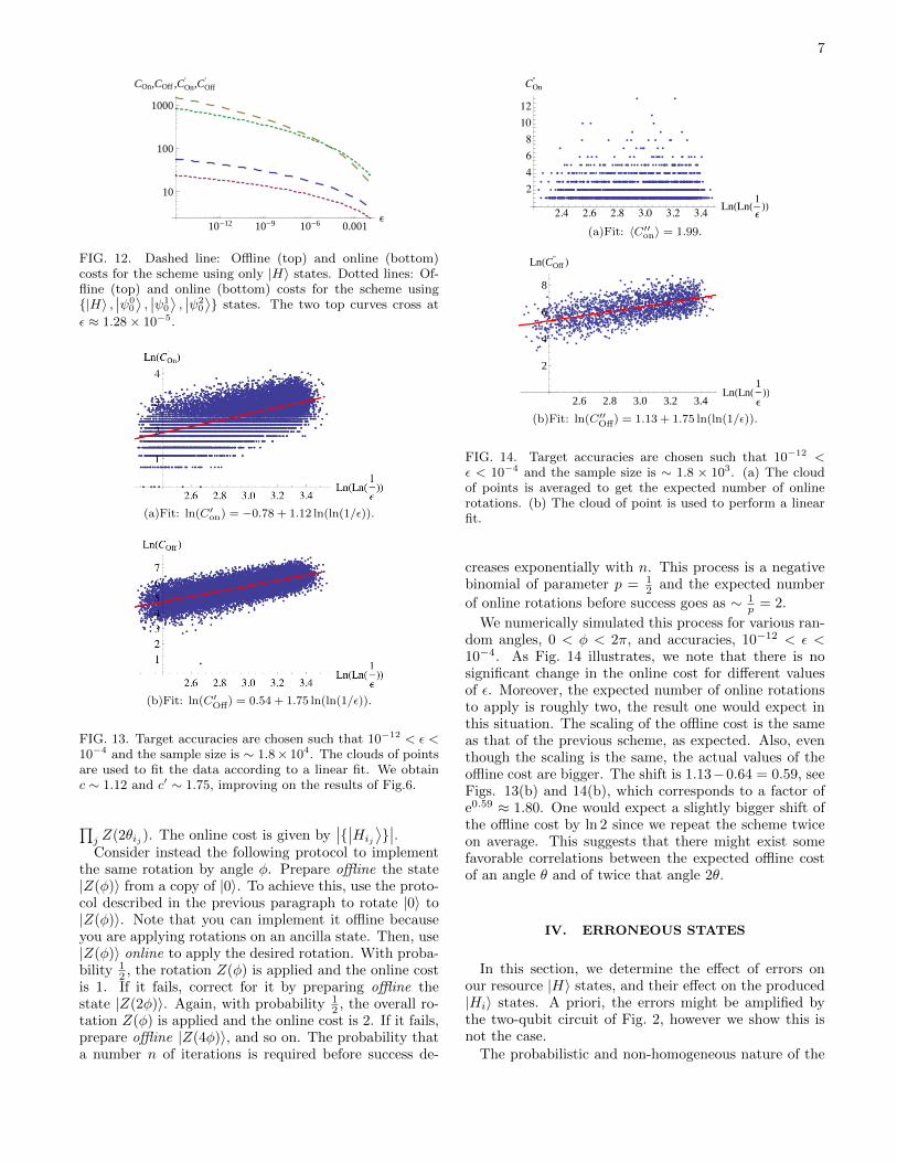
However, the basic offline costs of our new states∣∣ψi0⟩ are significantly higher; for precision ∼ 10−4, eventhough the online cost is smaller using the new states,the offline cost is still smaller if we restrict ourselves tothe simpler scheme using only |H〉 states. For the proto-col using the new input states to reduce both the onlineand offline costs, we need to consider precisions smallerthen ε ≈ 1.28× 10−5, see Fig. 12.

The reason why we do not consider other measurementoutcomes in the circuits considered in this section is thatin general, potential errors on the |H〉 states are amplifiedby the circuit. Output states in these cases might stillprove useful, but a careful analysis of the evolution oferrors must be conducted.

2 4 6 8 10i10-4

0.001

0.01

0.1

1Θ

FIG. 10. Dots: States obtainable by recursively using thecircuit of Fig. 2 with initial resource states |H〉,

∣∣ψ0⟩,∣∣ψ1

⟩and

∣∣ψ2⟩.

Π

4

Π

8Π

16 Π

32Π

64

ÈH0>

ÈH1>

ÈΨ02

>

ÈΨ12

>

ÈΨ01

>

ÈΨ11

>

ÈΨ00

>

ÈΨ10

> …

FIG. 11. Dots: Rotations implementable using |Hi〉,∣∣ψ0

i

⟩,∣∣ψ1

i

⟩,∣∣ψ2

i

⟩states.

B. Minimizing the online cost

In this section, we aim to minimize the online cost, atthe price of potentially increasing the offline cost.

The protocol up to this point can be summarized asfollows. Suppose one wants to implement a Z-rotationof an arbitrary angle φ on a logical state |ψ〉. One hasto implement a sequence of j rotations {Z(2θij )} on |ψ〉using the sequence of states {

∣∣Hij

⟩}, such that Z(φ) ≈

i 2θi 2φ0i 2φ1

i 2φ2i

0 7.853× 10−1 4.456× 10−1 5.698× 10−1 6.898× 10−1

1 3.398× 10−1 1.871× 10−1 2.415× 10−1 2.954× 10−1

2 1.419× 10−1 7.770× 10−2 1.004× 10−1 1.231× 10−1

3 5.886× 10−2 3.220× 10−2 4.162× 10−2 5.105× 10−2

4 2.439× 10−2 1.334× 10−2 1.724× 10−2 2.115× 10−2

5 1.010× 10−2 5.525× 10−3 7.142× 10−3 8.761× 10−3

6 4.184× 10−3 2.288× 10−3 2.959× 10−3 3.629× 10−3

7 1.733× 10−3 9.479× 10−4 1.225× 10−3 1.503× 10−3

8 7.179× 10−4 3.926× 10−4 5.076× 10−4 6.226× 10−4

TABLE IV. Rotations implementable using|Hi〉 ,

∣∣ψ0i

⟩,∣∣ψ1

i

⟩,∣∣ψ2

i

⟩states.

7

10-12 10-9 10-6 0.001Ε

10

100

1000

COn,COff ,COn' ,COff

'

FIG. 12. Dashed line: Offline (top) and online (bottom)costs for the scheme using only |H〉 states. Dotted lines: Of-fline (top) and online (bottom) costs for the scheme using{|H〉 ,

∣∣ψ00

⟩,∣∣ψ1

0

⟩,∣∣ψ2

0

⟩} states. The two top curves cross at

ε ≈ 1.28× 10−5.

(a)Fit: ln(C′on) = −0.78 + 1.12 ln(ln(1/ε)).

(b)Fit: ln(C′Off) = 0.54 + 1.75 ln(ln(1/ε)).

FIG. 13. Target accuracies are chosen such that 10−12 < ε <10−4 and the sample size is ∼ 1.8× 104. The clouds of pointsare used to fit the data according to a linear fit. We obtainc ∼ 1.12 and c′ ∼ 1.75, improving on the results of Fig.6.

∏j Z(2θij ). The online cost is given by

∣∣{∣∣Hij

⟩}∣∣.

Consider instead the following protocol to implementthe same rotation by angle φ. Prepare offline the state|Z(φ)〉 from a copy of |0〉. To achieve this, use the proto-col described in the previous paragraph to rotate |0〉 to|Z(φ)〉. Note that you can implement it offline becauseyou are applying rotations on an ancilla state. Then, use|Z(φ)〉 online to apply the desired rotation. With proba-bility 1

2 , the rotation Z(φ) is applied and the online costis 1. If it fails, correct for it by preparing offline thestate |Z(2φ)〉. Again, with probability 1

2 , the overall ro-tation Z(φ) is applied and the online cost is 2. If it fails,prepare offline |Z(4φ)〉, and so on. The probability thata number n of iterations is required before success de-

2.4 2.6 2.8 3.0 3.2 3.4 Ln!Ln!1!""2

4681012

COn''

(a)Fit: 〈C′′on〉 = 1.99.

2.6 2.8 3.0 3.2 3.4LnHLnH

1

Ε

LL

2

4

6

8

LnHCOff'' L

(b)Fit: ln(C′′Off) = 1.13 + 1.75 ln(ln(1/ε)).

FIG. 14. Target accuracies are chosen such that 10−12 <ε < 10−4 and the sample size is ∼ 1.8 × 103. (a) The cloudof points is averaged to get the expected number of onlinerotations. (b) The cloud of point is used to perform a linearfit.

creases exponentially with n. This process is a negativebinomial of parameter p = 1

2 and the expected number

of online rotations before success goes as ∼ 1p = 2.

We numerically simulated this process for various ran-dom angles, 0 < φ < 2π, and accuracies, 10−12 < ε <10−4. As Fig. 14 illustrates, we note that there is nosignificant change in the online cost for different valuesof ε. Moreover, the expected number of online rotationsto apply is roughly two, the result one would expect inthis situation. The scaling of the offline cost is the sameas that of the previous scheme, as expected. Also, eventhough the scaling is the same, the actual values of theoffline cost are bigger. The shift is 1.13−0.64 = 0.59, seeFigs. 13(b) and 14(b), which corresponds to a factor ofe0.59 ≈ 1.80. One would expect a slightly bigger shift ofthe offline cost by ln 2 since we repeat the scheme twiceon average. This suggests that there might exist somefavorable correlations between the expected offline costof an angle θ and of twice that angle 2θ.

IV. ERRONEOUS STATES

In this section, we determine the effect of errors onour resource |H〉 states, and their effect on the produced|Hi〉 states. A priori, the errors might be amplified bythe two-qubit circuit of Fig. 2, however we show this isnot the case.

The probabilistic and non-homogeneous nature of the

8

ææ

ææ

ææ

ææ

ææ

ææ

ææ

ææ

ææ

ææ

æ

æ

ææ

æ

æ

æ

æ

àà

àà

àà

àà

àà

àà

àà

àà

àà

àà

à

à

ìì

ìì

ìì

ìì

ìì

ìì

ìì

ìì

5 10 15 20 25i

10-10

10-7

10-4

0.1

DHΡi,ΡiaL

FIG. 15. Evolution of the trace distance between imperfectρai and perfect |Hi〉 states. Circles: data for p = 10−4, 1 ≤i ≤ 28. Squares: data for p = 10−6, 1 ≤ i ≤ 22. Diamonds:data for p = 10−8, 1 ≤ i ≤ 16. The full lines are exponentialdecay fits: (2.08 ∗ 10−3) × 2.31−i using points 18 ≤ i ≤ 28,(1.63 ∗ 10−5) × 2.28−i using points 18 ≤ i ≤ 22 and (1.26 ∗10−7)× 2.24−i using points 13 ≤ i ≤ 16 for the circle, squareand diamond data set, respectively. Sample size is 1000. Weconclude that if the initial resource state has desired accuracy,then this is also true of all derived resource states.

presented protocol is not well suited for an analyticalstudy of the evolution of errors on |Hi〉 states. Instead,we rely on a numerical study for three different types oferrors. We use the trace distance on states ρ and σ,

D(ρ, σ) =1

2tr(√

(ρ− σ)†(ρ− σ)),

to measure the accuracy of the imperfect |Hi〉 states. Weassume Clifford operations are perfect and that errors canonly occur on the |H〉 states.

We consider three types of erroneous states. First, weassume that the mixed state, ρa0 , is perfectly along theline joining the center of the Bloch sphere and the theperfect state, i.e.,

ρa0(p) = (1− p)|H0〉〈H0|+ p| −H0〉〈−H0|,

where |−H0〉 = sin π8 |0〉−cos π8 |1〉 is the state orthogonal

to |H0〉. We denote the imperfect version of |Hi〉 obtainedfrom ρa0 states as ρai . If Clifford operations are perfect,we can always bring any mixed state into this form usingtwirling [12]. However, for the protocol to be of practicalinterest, we require it to remain stable under the twofollowing types of errors, where we assume that the stateis pure, but that the rotation is slightly off of the desiredaxis by δ:

ρb0(δ) =1

2

(I + sin

(π4

+ δ)X + cos

(π4

+ δ)Z)

ρc0(δ) =1

2

(I + sin

π

4cos δX + sin

π

4sin δY + cos

π

4Z).

We numerically generated pseudo-random instances ofthe scheme to produce |Hi〉 states for different values ofi and for different noise strengths. We considered 1000instances for each of the three types of errors and noisestrengths 10−4, 10−6 and 10−8. Figures 15 and 16 showthat the protocol actually reduces the amplitude of pos-sible errors on the resource |H〉 states, such that if we

æ ææ

ææ

ææ

ææ

ææ

ææ

ææ

ææ

ææ

ææ

ææ

ææ

ææ

æ

à àà

àà

àà

àà

àà

àà

àà

àà

àà

àà

à

ì ìì

ìì

ìì

ìì

ìì

ìì

ìì

ì

5 10 15 20 25i

10-10

10-7

10-4

0.1

DHΡi,ΡibL

(a)Fits: (1.17 ∗ 10−3)× 2.31−i,(1.03 ∗ 10−5)× 2.29−i and

(7.50 ∗ 10−8)× 2.25−i

æ ææ

ææ

ææ

ææ

ææ

ææ

ææ

ææ

ææ

ææ

ææ

ææ

ææ

æ

à àà

àà

àà

àà

àà

àà

àà

àà

àà

àà

à

ì ìì

ìì

ìì

ìì

ìì

ìì

ìì

ì

5 10 15 20 25i

10-10

10-7

10-4

0.1

DHΡi,ΡicL

(b)Fits: (8.28 ∗ 10−4)× 2.31−i,(7.32 ∗ 10−6)× 2.30−i and

(5.30 ∗ 10−8)× 2.25−i

FIG. 16. Distances between the ideal |Hi〉 states and theimperfects states ρbi and ρci respectively. Sample size is 1000.ε = 10−4, 10−6, 10−8 in both cases.

start with |H〉 meeting our target accuracy, all the sub-sequent derived |Hi〉 states will also meet it. This evensuggests that for bigger values of i, one could use noisier|H〉 states and still achieve the desired accuracy. Thiscould make a dramatic difference if it enables one to re-duce the number of distillation recursions necessary toprepare the |H〉 states.

We note a very similar behavior for the three types oferrors. The exponential decay of the distance betweenerroneous and ideal states confirms that the errors arewell behaved under the proposed protocol. We note thatthe bases for the exponential decay of the errors are com-parable, but smaller, than the basis for the exponentialdecay of the angle implemented. So, for a given errorrate, there exits a point where the angle of rotation im-plemented by |Hi〉 for some i is going to be comparableor smaller to the error on that angle. However, this isnot a problem in practice since for, e.g., ε ∼ 10−4, wefind i = 150. For this value of i the angle is θi ∼ 10−57.

V. COMPARISON TO SOLOVAY-KITAEVDECOMPOSITION

In this section, we compare the performance of theSolovay-Kitaev decomposition of [16] and that of the

9

10!15 10!12 10!9 10!6 0.001"

10

100

1000

10000

100000CSKZ ,COnZ ,COffZ

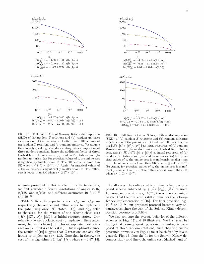
(a)ln(CZ

SK) = −4.88 + 4.41 ln(ln(1/ε))

ln(CZOn) = −0.49 + 1.29 ln(ln(1/ε))

ln(CZOff) = −0.72 + 2.27 ln(ln(1/ε))

10!15 10!12 10!9 10!6 0.001"

100

1000

1000010000

CSK,COn,COff

(b)ln(CSK) = −2.67 + 3.40 ln(ln(1/ε))

ln(COn) = −0.49 + 1.29 ln(ln(1/ε)) + ln 3ln(COff) = −0.72 + 2.27 ln(ln(1/ε)) + ln 3

FIG. 17. Full line: Cost of Solovay Kitaev decompostion(SKD) of (a) random Z-rotations and (b) random unitariesas a function of the precision ε. Dotted line: Offline costs of(a) random Z-rotations and (b) random unitaries. We assumethat, loosely speaking, a random unitary is the composition ofthree random rotations, hence the additional factor of three.Dashed line: Online cost of (a) random Z-rotations and (b)random unitaries. (a) For practical values of ε, the online costis significantly smaller than SK. The offline cost is lower thanSK when ε ≤ 8.71 × 10−4. (b) Again, for practical values ofε, the online cost is significantly smaller than SK. The offlinecost is lower than SK when ε ≤ 2.67× 10−7.

schemes presented in this article. In order to do this,we first consider different Z-rotations of angles π/16,π/128, and π/1024 and different accuracies 10−4, 10−8

and 10−12.

Table V lists the expected costs. Con and Coff arerespectively the online and offline costs to implementthe gate using only |H〉 states. C ′on and C ′off referto the costs for the version of the scheme thats uses{|H〉 ,

∣∣ψ00

⟩,∣∣ψ1

0

⟩,∣∣ψ2

0

⟩} as initial resource states. CSK

refers to the extrapolated cost to implement these gatesusing the results from [16]. This extrapolated cost aver-ages over all unitaries (c ∼ 3.40). This is optimistic sincethe results of [16] suggest that Z-rotations are actuallyharder to implement (c ∼ 4.3). Note that in theory, thecost of this algorithm is O(logc(1/ε), where c = 3.97 [14].

10!15 10!12 10!9 10!6 0.001"

10

100

1000

10000

100000CSKZ ,COn'#Z ,COff'#Z

(a)ln(C′ZSK) = −4.88 + 4.41 ln(ln(1/ε))

ln(C′ZOn) = −0.78 + 1.12 ln(ln(1/ε))

ln(C′ZOff) = 0.54 + 1.75 ln(ln(1/ε))

10!15 10!12 10!9 10!6 0.001"

10

100

1000

10000

CSK,COn' ,COff'

(b)ln(C′SK) = −2.67 + 3.40 ln(ln(1/ε))

ln(C′On) = −0.78 + 1.12 ln(ln(1/ε)) + ln 3ln(C′Off) = 0.54 + 1.75 ln(ln(1/ε)) + ln 3

FIG. 18. Full line: Cost of Solovay Kitaev decompostion(SKD) of (a) random Z-rotations and (b) random unitariesas a function of the precision ε. Dotted line: Offline costs, us-ing {|H〉 ,

∣∣ψ0⟩,∣∣ψ1

⟩,∣∣ψ2

⟩} as initial resources, of (a) random

Z-rotations and (b) random unitaries. Dashed line: Onlinecost, using {|H〉 ,

∣∣ψ0⟩,∣∣ψ1

⟩,∣∣ψ2

⟩} as initial resources, of (a)

random Z-rotations and (b) random unitaries. (a) For prac-tical values of ε, the online cost is significantly smaller thanSK. The offline cost is lower than SK when ε ≤ 4.41 × 10−4.(b) Again, for practical values of ε, the online cost is signif-icantly smaller than SK. The offline cost is lower than SKwhen ε ≤ 1.03× 10−6.

In all cases, the online cost is minimal when our pro-posed scheme enhanced by {

∣∣ψ00

⟩,∣∣ψ1

0

⟩,∣∣ψ2

0

⟩} is used.

For rougher precision, e.g., 10−4, the offline cost mightbe such that the total cost is still minimal for the Solovay-Kitaev implementation of [16]. For finer precision, e.g.,10−8 or 10−12, our proposed protocol becomes very ad-vantageous, since the cost of the Solovay-Kitaev decom-position becomes prohibitive.

We also compare the average behavior of the differentschemes as Figs. 17 and 18 illustrate. We first start bynoting that, loosely speaking, a random unitary is com-posed of three random rotations, such that the curvespresented previously in Fig. 12 must be shifted by ln 3 ingeneral. Fig. 17 plots the fit for the Solovay-Kitaev de-composition (solid line), the online cost (dashed) and of-

10

θ C ε = 10−4 ε = 10−8 ε = 10−12

π/16 CSK 43.83 2646 29120Con 10.20 24.52 41.95C′on 5.88 12.48 19.38Coff 73.06 349.8 874.4C′off 98.29 306.1 595.0

π/128 CSK 53.84 2879 29530Con 5.47 18.96 39.27C′on 3.32 9.27 16.91Coff 49.18 313.0 923.9C′off 52.60 234.1 560.8

π/1024 CSK 128.1 2594 15075Con 7.99 23.08 42.93C′on 3.00 8.37 15.23Coff 77.42 381.3 969.1C′off 65.75 245.5 530.7

TABLE V. Con and Coff are respectively the online and offlinecosts to implement the Z-rotation by angle θ using only |H〉states, to precision ε. C′on and C′off refer to the costs for theversion of the scheme thats uses {|H〉 ,

∣∣ψ00

⟩,∣∣ψ1

0

⟩,∣∣ψ2

0

⟩} as

initial resource states. CSK refers to the extrapolated cost toimplement these gates using the results from [16].

fline cost (dotted). For all practical accuracies, the onlinecost of our proposed scheme is consistently the smallest.However, the offline cost becomes advantageous whenε < 8.71 × 10−4 for Z-rotations and ε < 2.67 × 10−7 forrandom unitaries. Fig. 18 plots the same for the schemewith additional initial resource states. Similarly, the of-fline cost becomes advantageous when ε < 4.41 × 10−4

for Z-rotations and ε < 1.03×10−6 for random unitaries.

VI. CONCLUSION

We have proposed an alternative protocol to Solovay-Kitaev decomposition that results in significantly smallerresource costs, in both the number of required resourcestates and the depth of the circuit. We have shown asignificant improvement on average in the value of c,and in many cases the number of distilled states androtations required to implement a single-qubit unitarygate are reduced. Another advantage of our protocol isthat the number of resources required is a “smoother”function of accuracy, whereas Solovay-Kitaev decompo-sition is step-like in nature because of the recursion pro-cess used in practice. However, note that our protocolsand Solovay-Kitaev decomposition are not exclusive. Itmight be that some unitaries are better implemented us-ing Solovay-Kitaev decomposition, while our scheme isbetter suited for Z-rotations, which occur, among otheralgorithms, in the quantum Fourier transform.

As future research, there are likely a variety of othercircuits that enable other “ladders” of states. One natu-ral extension would be to use the SH eigenstates distilledusing the protocols of [11, 13]. Another extension wouldbe to perform a systematic study of “small” Clifford cir-cuits. Finally, we note that implementing a rotation bychoosing the state which results in an angle closest to thetarget angle is a simple way of achieving our goal, but itis surely suboptimal. An important research directionwould be to optimize the sequence of angles required toimplement the desired rotation.

VII. ACKNOWLEDGEMENTS

We thank Alex Bocharov for many useful discussions.

[1] A. Kitaev, Ann. Phys. 303 (2003), arxiv:quant-ph/9707021.

[2] M. H. Freedman, Proc. Natl. Acad. Sci. 95 (1998).[3] J. Preskill, in Introduction to Quantum Computation,

edited by H.-K. Lo, S. Popescu, and T. Spiller (1998)arxiv:quant-ph/9712048.

[4] M. H. Freedman, M. Larsen, and Z. Wang, Commun.Math. Phys. 227 (2002), arxiv:quant-ph/0001108.

[5] C. Nayak, S. Simon, A. Stern, M. Freedman, and S. D.Sarma, Rev. Mod. Phys. 80 (2008), arXiv:0707.1889.

[6] H. Bombin and M. A. Martin-Delgado, Journal ofPhysics A Mathematical General 42, 095302 (2009),arXiv:0704.2540 [quant-ph].

[7] A. G. Fowler, A. M. Stephens, and P. Groszkowski, Phys.Rev. A 80 (2009).

[8] D. Gottesman, The Heisenberg Representation ofQuantum Computers, Ph.D. thesis, Caltech (1998),

arXiv:quant-ph/9807006v1.[9] S. Aaronson and D. Gottesman, Phys. Rev. A 70, 052328

(2004), arXiv:quant-ph/0406196.[10] M.A.Nielsen and I.L.Chuang, Quantum Computation

and Quantum Information (Cambridge University Press,Cambridge, UK, 2000).

[11] S. Bravyi and A. Kitaev, Phys. Rev. A 71, 022316 (2005).[12] A. M. Meier, B. Eastin, and E. Knill, arXiv:1204.4221v1

(2012).[13] S. Bravyi and J. Haah, (2012), 1209.2426.[14] C. M. Dawson and M. A. Nielsen, (2005).[15] A. Kitaev et al., Classical and Quantum Computation

(American Mathematical Society, Providence, RI, 2002).[16] A. Bocharov and K. M. Svore, arXiv:1206.3223v1 (2012).