a statistically identifiable model for tensor-valued
TRANSCRIPT

1
A Statistically Identifiable Model for Tensor-ValuedGaussian Random Variables
Bruno Scalzo Dees, Student Member, IEEE, Anh-Huy Phan, Member, IEEE, Danilo P. Mandic, Fellow, IEEE
Abstract—Real-world signals typically span across multipledimensions, that is, they naturally reside on multi-way datastructures referred to as tensors. In contrast to standard “flat-view” multivariate matrix models which are agnostic to datastructure and only describe linear pairwise relationships, weintroduce the tensor-valued Gaussian distribution which catersfor multilinear interactions – the linear relationship betweenfibers – which is reflected by the Kronecker separable struc-ture of the mean and covariance. By virtue of the statisticalidentifiability of the proposed distribution formulation, wherebydifferent parameter values strictly generate different probabilitydistributions, it is shown that the corresponding likelihoodfunction can be maximised analytically to yield the maximumlikelihood estimator. For rigour, the statistical consistency of theestimator is also demonstrated through numerical simulations.The probabilistic framework is then generalised to describe thejoint distribution of multiple tensor-valued random variables,whereby the associated mean and covariance exhibit a Khatri-Rao separable structure. The proposed models are shown to serveas a natural basis for gridded atmospheric climate modelling.
Index Terms—Gaussian, Khatri-Rao separability, Kroneckerseparability, maximum likelihood estimation, tensors.
I. INTRODUCTION
Tensor data structures are gaining increasing prominence inmodern Data Analytics, especially in relation to the Big Dataparadigm where, equipped with the power of their underlyingmultilinear algebra, they provide a rich analysis platformfor making sense from multidimensional data. In particular,tensor decompositions have experienced a surge in popularityowing to their role as high-dimensional generalisations of the“flat-view” linear algebra paradigms, an example of which isthe tensor-valued higher-order singular value decomposition(HOSVD), a generic extension of the ordinary matrix SVD.The tensor data domain is amenable to such generalisations ofstandard matrix signal processing and machine learning tools[1], [2], [3], [4], [5]. Real-world applications of tensors includethose in chemometrics [6], fluid mechanics [7], geostatistics[8], magnetic resonance imaging [9], psychometrics [10],statistical mechanics [11], MIMO communications [12] andbiomedical applications [13].
In addition, the analysis of tensor-valued data through mul-tilinear algebra has been an enabling tool for solving criticalinformation representation and storage bottlenecks, namely thecurse of dimensionality. However, while multilinear algebraassumes some form of deterministic relation between dataentries, the interactions between real-world observables aretypically causal and probabilistic, including practical situations
B. Scalzo Dees and D. P. Mandic are with the Imperial College Lon-don, London SW7 2AZ, U.K. (e-mail: [email protected];[email protected]).
A.-H. Phan is with the Skolkovo Institute of Science and Technology,143026 Moscow, Russia (e-mail: [email protected]).
where even deterministic information is contaminated withrandom noise, missing or unreliable entries. This makes theexisting multilinear models inadequate for such scenarios,since the associated probability density functions are not yetwell defined for tensor-valued data. The consideration oftensor-valued tools within a rigorous probabilistic frameworkwould therefore offer a number of important advantages:
(i) Possibility for statistical and hypothesis testing throughthe likelihood function;
(ii) Opportunity to introduce Bayesian inference methods;(iii) Ability to employ class-conditional densities for classifi-
cation tasks;(iv) A framework to assess the degree of novelty of a new
data point, and input variable selection;(v) A rigorous probabilistic framework to deal with missing
data values;(vi) Straightforward consideration of a mixture of probabilis-
tic models.
While this has naturally motivated the developments of prob-abilistic tensor-valued models, owing to the ambiguity in theproblem formulation, a wide range of solutions have beenproposed. The tensor-valued Gaussian processes were firstproposed in [14] as a means of obtaining a probabilisticvariant of the Tucker decomposition which can handle missingdata entries. The work in [15] further proposed a hierarchicalBayesian extension to the Tucker decomposition. The basicproperties of the distribution, such as the marginal and condi-tional distributions, moments, and characteristic function, werelater derived in [16]. However, all these methods are, in somesense, extensions of the matrix-valued Gaussian distributionwith Kronecker separable covariance matrix [17], [18], [19].
Several remaining issues need to be addressed prior toa more widespread application of the class of probabilistictensor-valued models. For example, existing parameter esti-mation procedures for tensor-valued Gaussian distributions areiterative, such as the expectation-maximization algorithm [14],[20] or the block coordinate descent [21], [15], [22], [23],also referred to as the flip-flop algorithm. Such techniquesare susceptible to local maxima and do not guarantee globaloptimality. A closely related topic is that of covariance matrixestimation with the Kronecker separable structure [24]. Twoasymptotically efficient estimation solutions have been pro-posed, the first being a variant of the well-known alternatingmaximization technique, while the second method is basedon covariance matching principles. However, these estimatorswere derived only for the Kronecker product of two matrices,and were not considered within the tensor-valued setting.
arX
iv:1
911.
0291
5v5
[ee
ss.S
P] 3
Dec
201
9

2
This all points out that there is a need for a general classof estimators, derived in a closed-form in the tensor domain,which would guarantee global optimality of probabilistic esti-mation procedures. In this way, the problem with the existingmodels which do not impose multilinear assumptions on thestructure of the mean would be resolved, a critical issue for acomplete characterisation of tensor-valued random variables.To this end, we derive a rigorous form of the tensor-valuedGaussian distribution and introduce its corresponding maxi-mum likelihood estimator in a closed-form. This is achievedthrough a novel statistically identifiable formulation of the dis-tribution, whereby different values of the parameters generatestrictly different probability distributions; this allows for theunderlying likelihood function to be maximised analytically,unlike the existing formulations. Moreover, we extend theproposed probabilistic framework to account for the jointdistribution of multiple tensor-valued random variables.
The rest of this paper is organized as follows. Section IIprovides a comprehensive introduction to multilinear algebra.Section III describes the underpinning Kronecker separablemean and covariance properties exhibited by tensor-valuedrandom variables. The proposed tensor-valued Gaussian dis-tribution and its maximum likelihood estimator are introducedin Section IV. The multivariate tensor-valued distribution isderived in Section V. An intuitive example of the proposedmodel applied to gridded atmospheric temperature modellingis provided in Section VI.
II. PRELIMINARIES
We follow the notation employed in [1], whereby scalarsare denoted by a lightface font, e.g. x; vectors by a lowercaseboldface font, e.g. x; matrices by a uppercase boldface font,e.g. X; and tensors by a boldface calligraphic font, e.g. X .
The order of a tensor defines the number of its dimensions,also referred to as modes, i.e. the tensor X ∈ RI1×···×IN hasN modes and K =
∏Nn=1 In elements in total.
Tensors can be reshaped into mathematically tractablelower-dimensional representations (unfoldings) which can bemanipulated using standard linear algebra. The vector unfold-ing, also known as vectorization, is denoted by
x = vec(X ) ∈ RK (1)
while the mode-n unfolding (matricization), denoted byX(n) ∈ RIn×
KIn , is obtained by reshaping a tensor into a
matrix in the form
X(n) =[
f(n)1 , f
(n)2 , . . . , f
(n)KIn
](2)
where the column vector, f(n)i ∈ RIn , is referred to as the i-th
mode-n fiber. Fibers are a multi-dimensional generalization ofmatrix rows and columns.
The operation of mode-n unfolding can be viewed as arearrangement of the mode-n fibers as column vectors ofthe matrix, X(n), as illustrated in Figure 1. Notice that theconsidered order-3 tensor, X , has alternative representationsin terms of mode-1 (left panel), mode-2 (middle panel) andmode-3 fibers (right panel), that is, its columns, rows and tubes.
n = 1 n = 2 n = 3
X
X(n)
Fig. 1: Mode-n matrix unfolding, X(n), of an order-3 tensor,X , as a rearrangement of the mode-n fibers, f
(n)i .
A. Tensor products
The Kronecker product between the matrices A ∈ RI×Iand B ∈ RJ×J yields a block matrix
A⊗B =
a11B · · · a1IB...
. . ....
aI1B · · · aIIB
∈ RIJ×IJ (3)
The Khatri-Rao product between two block matrices with Mrow and column partitions, A ∈ RMI×MI and B ∈ RMJ×MJ ,yields the block matrix A©∗B ∈ RMIJ×MIJ , with the (i, j)-thblock given by
A ©∗ B =
A11 ⊗B11 · · · A1M ⊗B1M
.... . .
...
AM1 ⊗BM1 · · · AMM ⊗BMM
(4)
The partial trace operator of a block matrix with M row andcolumn partitions, A ∈ RMI×MI , yields the block matrixptr (A) ∈ RM×M , with the (i, j)-th block given by
ptr (A) =
tr (A11) · · · tr (A1M )...
. . ....
tr (AM1) · · · tr (AMM )
(5)
The mode-n product of the tensor X ∈ RI1×···×IN with thematrix U ∈ RJn×In is denoted by
Y = X ×n U ∈ RI1×···×In−1×Jn×In+1×···×IN (6)
and is equivalent to performing the following steps:1: X(n) ← X . Mode-n unfold2: Y(n) ← UX(n) . Left matrix multiplication3: Y ← Y(n) . Re-tensorize
For convenience, we denote the sequence of Kronecker prod-ucts of the matrices U(n) ∈ RIn×In by
N⊗n=1
U(n) = U(1) ⊗ · · · ⊗U(N) ∈ RK×K (7)
and the sequence of Khatri-Rao products of the block matriceswith M row and column partitions, U(n) ∈ RMIn×MIn , by
N©∗n=1
U(n) = U(1) ©∗ · · · ©∗ U(N) ∈ RMK×MK (8)
The sequence of outer products of the vectors u(n) ∈ RIn is

3
denoted byN◦n=1
u(n) = u(1) ◦ · · · ◦ u(N) ∈ RI1×···×IN (9)
The sequence of mode-n products between the tensor X andthe matrices U(n) ∈ RJn×In is denoted by
Y = X N×n=1
U(n) = X ×1U(1)×2 · · ·×N U(N) ∈ RJ1×···×JN
(10)This operation can also be expressed in the mathematicallyequivalent vector and matrix representations, that is
y =
Å1⊗n=N
U(n)
ãx ∈ RL (11)
Y(n) = U(n)X(n)
Ñ1⊗i=Ni 6=n
U(i)T
é∈ RJn×
LJn (12)
where L =∏Nn=1 Jn. Figure 2 illustrates the sequence of
mode-n products of an order-3 tensor with matrices U(n).
Y = U(1)
X U(2)
U(3)
Fig. 2: Sequence of mode-n products for n = 1, 2, 3.
B. Tensor-valued statistical operators
For clarity, we shall first introduce the notation for thefirst- and second-order tensor-valued statistical operators. Theoperation of taking the expectation of a random tensor, X , isequal to the element-wise expectation, which yields the meantensor M = E {X}. The variance of X is then defined as
var {X} = E{‖X −M‖2
}= E
{‖S‖2} (13)
that is, the expected squared Frobenius norm of the centredtensor variable, S = X −M. Using the mode-n unfoldingrepresentation in (2) based on fibers, we can now define themode-n fiber covariance through the total expectation theorem[25] as follows
cov¶f (n)©= Ei
¶cov¶f(n)i
©©= E
¶S(n)S
T(n)
©(14)
where Ei{·} denotes the expectation over the indices i. Wealso denote this operation by cov
{X(n)
}≡ cov
{f (n)
}.
III. KRONECKER SEPARABLE STATISTICS
In standard multivariate data analysis, multiple measure-ments are collected at a given trial, experiment or time instant,to form a vector-valued data sample, x ∈ RK . An assumptioninherently adopted in statistical modeling is that the variablesare described by the probability distribution, x ∼ N (m,R),which implies that the mean vector, m ∈ RK , and covariancematrix, R ∈ RK×K , are unstructured. However, if the vari-ables have a natural tensor representation, then it is desirable,and even necessary, to assume that the mean and covariance
exhibit a more structured form motivated by physical consid-erations. It then naturally follows that the statistical propertiesof tensor-valued random variables are directly linked to thoseof separable Gaussian random fields – the continuous-spacecounterpart of tensors – introduced in the next section.
A. Separable Gaussian random fields
A Gaussian random field in an N -dimensional orthogonalcoordinate system is given by x : RN 7→ R, and is describedby the coordinate-dependent distribution
x(z) ∼ N(m(z), σ2(z)
)(15)
where z = {z(1), ..., z(N)} ∈ RN is an N -dimensionalcoordinate vector, and z(n) ∈ R is the n-th axis coordinate.Furthermore, such a random variable is equipped with acovariance operator, denoted by σ : RN × RN 7→ R, whichyields
σ(z1, z2) = cov {x(z1), x(z2)} (16)
where σ(z, z) ≡ σ2(z). A random variable is said to exhibita separable mean and covariance structure if and only if themean and covariance operators are linearly separable, that is
m(z) =N∏n=1
m(n)(z(n)), ∀z ∈ RN (17)
σ(z1, z2) =N∏n=1
σ(n)(z(n)1 , z
(n)2 ), ∀z1, z2 ∈ RN (18)
where m(n) : R 7→ R and σ(n) : R × R 7→ R are the meanand covariance operators specific to the n-th coordinate axis.
Remark 1. Real-world examples of fields in N -dimensionalcoordinates that are typically analysed using signal processingand machine learning techniques include:
(i) meteorological measurements in the longitude × latitude× altitude space;
(ii) colored pixels in the column × row × (R, G, B) space;(iii) time-frequency multichannel signals which reside in the
time × frequency × channel space.
Remark 2. Orthogonal coordinate systems that are mostcommonly found in Physics and Engineering include theCartesian, spherical polar, and cylindrical polar systems. Whilethe reason to prefer orthogonal coordinates over general curvi-linear coordinates is their simplicity, complications typicallyarise when coordinates are not orthogonal, for instance, inorthogonal coordinates problems can be solved by separationof variables, which reduces a single N -dimensional probleminto N single-dimensional problems. Tensors are naturallyendowed with this powerful property.
Remark 3. A function that is linearly separable in a givencoordinate system need not remain separable upon a change ofthe coordinate system. This asserts that the coordinate systemused for tensorizing a sampled field should be chosen so asto match the properties of the underlying physics. We nextintroduce the necessary tensorization condition to guaranteeseparability, which we refer to as topological coherence.
4
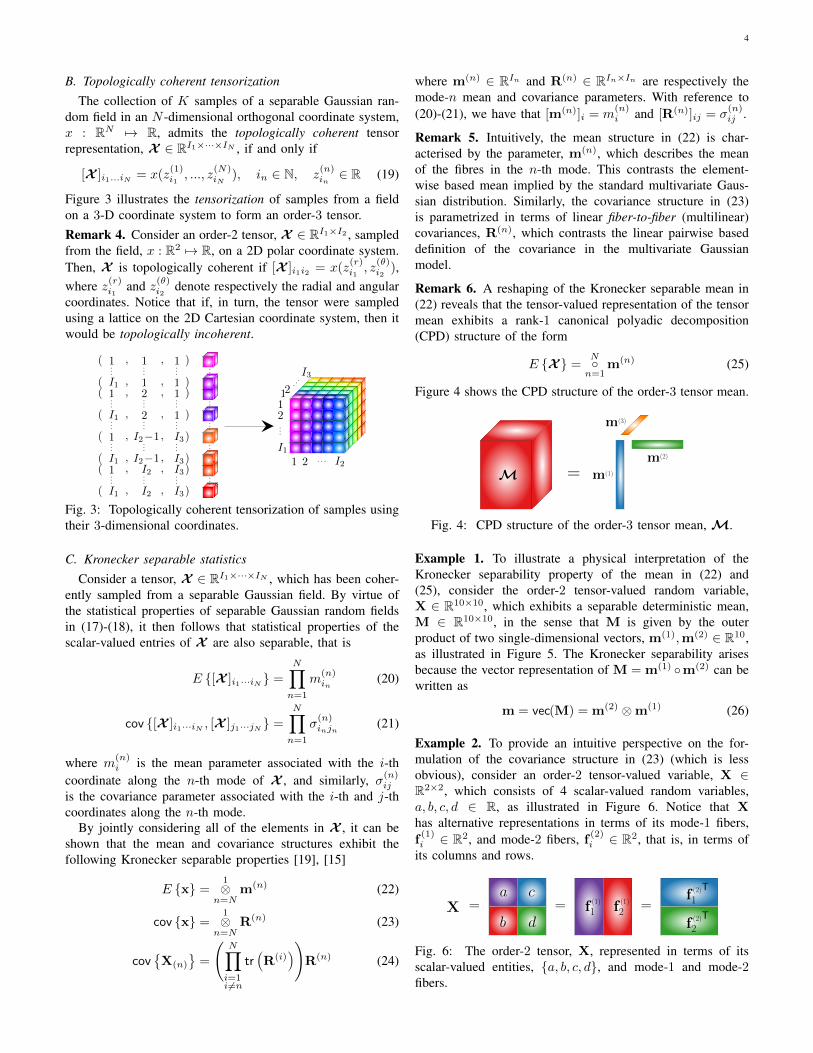
B. Topologically coherent tensorizationThe collection of K samples of a separable Gaussian ran-
dom field in an N -dimensional orthogonal coordinate system,x : RN 7→ R, admits the topologically coherent tensorrepresentation, X ∈ RI1×···×IN , if and only if
[X ]i1...iN = x(z(1)i1, ..., z
(N)iN
), in ∈ N, z(n)in∈ R (19)
Figure 3 illustrates the tensorization of samples from a fieldon a 3-D coordinate system to form an order-3 tensor.Remark 4. Consider an order-2 tensor, X ∈ RI1×I2 , sampledfrom the field, x : R2 7→ R, on a 2D polar coordinate system.Then, X is topologically coherent if [X ]i1i2 = x(z
(r)i1, z
(θ)i2
),where z(r)i1
and z(θ)i2denote respectively the radial and angular
coordinates. Notice that if, in turn, the tensor were sampledusing a lattice on the 2D Cartesian coordinate system, then itwould be topologically incoherent.
( 1 , 1 , 1 )...
......
...
( I1 , 1 , 1 )( 1 , 2 , 1 )
......
......
( I1 , 2 , 1 )...
......
...
( 1 , I2−1, I3)......
......
( I1 , I2−1, I3)( 1 , I2 , I3)...
......
...
( I1 , I2 , I3)
12...
I11 2 · · · I2
12· · ·I3
Fig. 3: Topologically coherent tensorization of samples usingtheir 3-dimensional coordinates.
C. Kronecker separable statisticsConsider a tensor, X ∈ RI1×···×IN , which has been coher-
ently sampled from a separable Gaussian field. By virtue ofthe statistical properties of separable Gaussian random fieldsin (17)-(18), it then follows that statistical properties of thescalar-valued entries of X are also separable, that is
E {[X ]i1···iN } =N∏n=1
m(n)in
(20)
cov {[X ]i1···iN , [X ]j1···jN } =N∏n=1
σ(n)injn
(21)
where m(n)i is the mean parameter associated with the i-th
coordinate along the n-th mode of X , and similarly, σ(n)ij
is the covariance parameter associated with the i-th and j-thcoordinates along the n-th mode.
By jointly considering all of the elements in X , it can beshown that the mean and covariance structures exhibit thefollowing Kronecker separable properties [19], [15]
E {x} =1⊗n=N
m(n) (22)
cov {x} =1⊗n=N
R(n) (23)
cov{X(n)
}=
(N∏i=1i 6=n
trÄR(i)ä)
R(n) (24)
where m(n) ∈ RIn and R(n) ∈ RIn×In are respectively themode-n mean and covariance parameters. With reference to(20)-(21), we have that [m(n)]i = m
(n)i and [R(n)]ij = σ
(n)ij .
Remark 5. Intuitively, the mean structure in (22) is char-acterised by the parameter, m(n), which describes the meanof the fibres in the n-th mode. This contrasts the element-wise based mean implied by the standard multivariate Gaus-sian distribution. Similarly, the covariance structure in (23)is parametrized in terms of linear fiber-to-fiber (multilinear)covariances, R(n), which contrasts the linear pairwise baseddefinition of the covariance in the multivariate Gaussianmodel.
Remark 6. A reshaping of the Kronecker separable mean in(22) reveals that the tensor-valued representation of the tensormean exhibits a rank-1 canonical polyadic decomposition(CPD) structure of the form
E {X} = N◦n=1
m(n) (25)
Figure 4 shows the CPD structure of the order-3 tensor mean.
M = m(1)
m(2)
m(3)
Fig. 4: CPD structure of the order-3 tensor mean, M.
Example 1. To illustrate a physical interpretation of theKronecker separability property of the mean in (22) and(25), consider the order-2 tensor-valued random variable,X ∈ R10×10, which exhibits a separable deterministic mean,M ∈ R10×10, in the sense that M is given by the outerproduct of two single-dimensional vectors, m(1),m(2) ∈ R10,as illustrated in Figure 5. The Kronecker separability arisesbecause the vector representation of M = m(1) ◦m(2) can bewritten as
m = vec(M) = m(2) ⊗m(1) (26)
Example 2. To provide an intuitive perspective on the for-mulation of the covariance structure in (23) (which is lessobvious), consider an order-2 tensor-valued variable, X ∈R2×2, which consists of 4 scalar-valued random variables,a, b, c, d ∈ R, as illustrated in Figure 6. Notice that Xhas alternative representations in terms of its mode-1 fibers,f(1)i ∈ R2, and mode-2 fibers, f
(2)i ∈ R2, that is, in terms of
its columns and rows.
Xa c
b d
f (2)T1
f (2)T2
f (1)
1 f (1)
2= = =
Fig. 6: The order-2 tensor, X, represented in terms of itsscalar-valued entities, {a, b, c, d}, and mode-1 and mode-2fibers.

5
(a) Tensor mean, M = m(1) ◦m(2) ∈ R10×10.
(b) m(1) ∈ R10. (c) m(2) ∈ R10.
Fig. 5: The Kronecker separable mean of an order-2 tensorvariable, X ∈ R10×10. (a) The tensor mean, M ∈ R10×10. (b)The mode-1 mean component, m(1) ∈ R10. (c) The mode-2mean component, m(2) ∈ R10.
The tensor, X, can also be described using its vector andmode-n unfolded representations, as shown in Figure 7.
x
a
b
c
d
= X(1) f (1)
1 f (1)
2= X(2) f (2)
1 f (2)
2=
Fig. 7: The vector (left panel), mode-1 unfolding (middlepanel) and mode-2 unfolding (right panel) representations ofthe order-2 tensor, X in Figure 6.
The mean of the vector representation of X is given by
E {x} =
ma
mb
mc
md
(27)
with its mean parameters taking the form
m(1) =
ñm
(1)1
m(1)2
ô(28)
m(2) =
ñm
(2)1
m(2)2
ô(29)
where, m(n)i = [m(n)]i. The separability condition on the
mean therefore asserts that
E {x} = m(2) ⊗m(1) =
m
(2)1 m
(1)1
m(2)1 m
(1)2
m(2)2 m
(1)1
m(2)2 m
(1)2
(30)
In turn, the covariance of each representation is given by
cov {x} =
σ2a σab σac σadσab σ2
b σbc σbdσac σbc σ2
c σcdσad σbd σcd σ2
d
(31)
cov¶f (1)©=
ñσ(1)11 σ
(1)12
σ(1)21 σ
(1)22
ô(32)
cov¶f (2)©=
ñσ(2)11 σ
(2)12
σ(2)21 σ
(2)22
ô(33)
where, σ(n)ij = [cov
{f (n)
}]ij denotes the covariance between
the i-th and j-th elements of the mode-n fibres, wherebyσ(n)ii ≡ σ
(n)2i . The separability condition on the covariance
then asserts that
cov {x} = cov¶f (2)©⊗ cov
¶f (1)©
(34)
that is
cov {x}=
σ(2)11 σ
(1)11 σ
(2)11 σ
(1)12 σ
(2)12 σ
(1)11 σ
(2)12 σ
(1)12
σ(2)11 σ
(1)12 σ
(2)11 σ
(1)22 σ
(2)12 σ
(1)12 σ
(2)12 σ
(1)22
σ(2)12 σ
(1)11 σ
(2)12 σ
(1)12 σ
(2)22 σ
(1)11 σ
(2)22 σ
(1)12
σ(2)12 σ
(1)12 σ
(2)12 σ
(1)22 σ
(2)22 σ
(1)12 σ
(2)22 σ
(1)22
(35)
Figure 8 further illustrates this concept, and shows thatwithin the unstructured multivariate representation (left panel)each pairwise covariance parameter is distinct. In turn, theKronecker separable representation (right panel) significantlyreduces the number of parameters required to describe theentire covariance structure, as indicated by a distinct colourassigned to each distinct parameter.
For instance, σ2a = σ
(2)11 σ
(1)11 asserts that the variance of a,
which resides in the first column and first row of X, is equalto the product of the variance parameters associated with thefirst row and first column. Similarly, σac = σ
(2)12 σ
(1)11 asserts
that the covariance between variables a and c is equal to theproduct of the covariance parameter shared by the first andsecond columns, σ(2)
12 , where a and c respectively reside, scaledby the variance parameter associated with the first row, σ(1)
11 ,where both variables reside.
a c
b d
σac
σab σcd
σbd
σbc
σad
σ2a σ2c
σ2b σ2d
a c
b d
σ(2)
12σ(1)
11
σ(2)
12σ(1)
22
σ(2)
11σ(1)
12 σ(2)
22σ(1)
12
σ(2)
12σ(1)
12
σ(2)
11σ(1)
11 σ(2)
22σ(1)
11
σ(2)
11σ(1)
22 σ(2)
22σ(1)
22
Fig. 8: Illustration of the covariance of a 2D tensor, X ,based on the unstructured multivariate case (left panel) andthe Kronecker separable case (right panel). Each distinctparameter is highlighted in a distinct color.

6
D. Parameter reduction through Kronecker separability
Observe that the unstructured mean vector, m ∈ RK ,contains K distinct parameters, whereas its Kronecker sep-arable counterpart, ⊗1
n=N m(n), reduces to∑Nn=1 In < K
parameters.Similarly, the unstructured covariance, R ∈ RK×K ,
consists of 12
(K2 +K
)distinct parameters, whereas its
Kronecker separable counterpart, ⊗1n=N R(n), reduces to
12
∑Nn=1
(I2n + In
)parameters.
Remark 7. The Kronecker separability conditions in (22)-(23) provide a rigorous and parsimonious alternative to theclassical unrestricted estimate of m and R, which is unstableor even unavailable if the dimensions of a data tensor are largecompared to the sample size.
Example 3. Consider a symmetric order-N tensor with allmodes of the same dimension, that is, In = I for all modesn, thereby containing K = IN elements in total. Then,the number of distinct parameters given by the unstructuredmultivariate Gaussian model and by its Kronecker separablecounterpart reduce respectively to
ηmulti =1
2
(I2N + 3IN
), η tensor =
N
2
(I2 + 3I
)(36)
Notice that with an increase in the order of the tensor, N , theratio of the respective distinct parameters, η tensor
η multi, approaches
zero in the limit for all I > 1, that is
limN→∞
η tensor
ηmulti= 0, I > 1 (37)
Figure 9 illustrates the immediate reduction in parametersresulting from an increase in the order of the tensor, N , whichdemonstrates the utility of tensor-valued models for alleviatingthe curse of dimensionality.
2 3 4 5 6 7 8 9 10I
0.0
0.2
0.4
0.6
0.8
1.0
η tensor
ηmulti
N = 1
N = 2
N = 3
N = 4
N = 5
Fig. 9: The ratio of distinct parameters between the structuredtensor model and the classical unstructured model, η tensor
η multi, for
a varying mode dimensionality, I , and tensor order, N .
IV. TENSOR-VALUED GAUSSIAN DISTRIBUTION
The Gaussian distribution has become a ubiquitous statis-tical model for describing the mean and covariance struc-ture of random variables observed across a broad varietyof disciplines. The material in Section III will now serveas background to derive the tensor-valued extension of theGaussian distribution, which can be used to describe the meanand covariance structure of multidimensional signals.
A. Related work
It has already been established that the tensor-valued ran-dom variable, X ∈ RI1×···×IN , exhibits a Gaussian distri-bution, defined by the tensor mean, M ∈ RI1×···×IN , andmode-n covariance, R(n) ∈ RIn×In , if and only if its vectorrepresentation, x ∈ RK , is distributed according to [15]
x ∼ NÅ
m,1⊗n=N
R(n)
ã(38)
where m = vec(M). With the condition in (38), it isstraightforward to show that the probability density functionof X is given by
p(X ) =expî− 1
2 (x−m)T(⊗1
n=N R(n)−1) (x−m)ó
(2π)K2 det
12(⊗1n=N R(n)
)(39)
The maximum likelihood (ML) estimator of the order-2 tensor(matrix) Gaussian parameters was first introduced in [21],and has been recently extended to the order-N tensor-valuedcase in [15]. The estimator is obtained by maximizing theassociated log-likelihood of observing T samples, denoted byX (t) ∈ RI1×···×IN , under the distribution in (39), that is
L =T−1∑t=0
ln p(X (t)
∣∣∣M, {R(n)}Nn=1
)(40)
The stationary points necessary to determine the ML estimatorare obtained upon setting the derivatives of L with respect toeach parameter to zero.
The expression for the stationary point with respect to thetensor mean, M, can be rearranged to yield the sample mean
M =1
T
T−1∑t=0
X (t) (41)
In turn, the stationary point obtained with respect to eachmode-n covariance parameter, R(n), does not lead to anestimator in closed-form. An iterative procedure based on theblock coordinate descent algorithm [21], [26], often referredto as the flip-flop algorithm, is therefore employed to approachthe ML estimate of R(n), given by
R(n) =InTK
T−1∑t=0
S(n)(t)
Ñ1⊗i=Ni 6=n
R(i)−1
éST(n)(t) (42)
where S(n) is the mode-n unfolding of the centred tensor-valued random variable, S = X −M.
It is important to notice that there exist several issues withthe existing formulation of the tensor Gaussian distribution:
(i) The global optimality of the iterative scheme in (42) isnot guaranteed with respect to the composition ⊗1
n=N R(n). Itis well known that the general class of alternating and cascadedschemes proposed for tensor-valued estimation problems, suchas the alternating least squares [27], [28] and tensor least meansquare [29], exhibit only local optimality. Global optimalitycan only be attained by evaluating the stationary point of Lwith respect to ⊗1
n=N R(n), as opposed to parallel evaluationsof R(n) for each n = 1, ..., N ;

7
(ii) The estimates, R(n), are non-identifiable, wherebydifferent values of the parameters may generate equivalentprobability distributions. Since the identifiability condition isabsolutely necessary for the ML estimator to be statisticallyconsistent [30], we can immediately conclude that the esti-mates obtained from the flip-flop algorithm are statistically in-consistent with respect to R(n) for all n. With this formulation,only the composition, ⊗1
n=N R(n), can be uniquely identified[21]. To see this, notice that an iterative solution can onlyestimate R(n) up to a multiplicative constant, e.g. by definingΘ(n) = aR(n) and Θ(m) = 1
aR(m), for any a 6= 0, we obtainthe same composition, since Θ(n) ⊗ Θ(m) = R(n) ⊗ R(m)
and so both estimates yield the same Kronecker product.(iii) The tensor mean, M, does not exhibit the separability
property in (25), which is required for a rigorous definitionof a tensor-valued variable which represent the discrete-spacecounterpart of the continuous separable Gaussian field.
B. The proposed statistically identifiable formulation
To resolve the aforementioned issues, we propose a newrepresentation-invariant formulation of the tensor-valued prob-ability distribution, based on the following rationale:
(i) The variance of the random tensor, X , is invariant to thedata representation, that is, for both the original data tensorand any of its unfoldings we have
var {X} = var {x} = var{X(n)
}, ∀n (43)
since the representations contain the same data entries. Con-sequently, the mode-n covariance parameters, R(n), shouldexhibit the same Frobenius norm for all modes n. Thiscontrasts the distribution formulation employed in [21], [15]which assumes that the variances at different modes can differ.In other words, in the existing formulation, the parametersR(n) are unconstrained.
A first step to resolving the non-identifiability issue is todissociate the magnitude of the variance from the covariancesparameters, {R(n)}Nn=1. This is achieved by introducing themode-n matrices, Θ(n) ∈ RIn×In , and the variance parameterσ2 ∈ R, to yield
1⊗n=N
R(n) = σ2
Å1⊗n=N
Θ(n)
ã(44)
where
σ2 = var {X} = tr
Å1⊗n=N
R(n)
ã(45)
A physically meaningful condition is to enforce the trace ofthe so introduced parameters, {Θ(n)}Nn=1, to have unit value,that is, tr
ÄΘ(n)
ä= 1, ∀n.
Intuitively, Θ(n) can be thought of as the covariance densityat the n-th mode, whereby its (i, j)-th element describes thepercentage of the total variance, σ2, assigned to the covariancebetween the i-th and j-th elements of the mode-n fiber,as shown in the sequel. Moreover, the unit-trace conditionsatisfies the definition in (45).
(ii) A rigorous definition of the tensor Gaussian variable,based on the statistical properties of separable Gaussian fields,
requires the mean to be separable, as in (25). Based on thearguments in point (i), we allow the mean to exhibit thefollowing separable structure
m = α
Å1⊗n=N
µ(n)
ã(46)
where α ∈ R is a positive scaling factor, and the vectorsµ(n) ∈ RIn are constrained to be unit vectors, i.e. ‖µ(n)‖ = 1for all n. In the tensor representation, this becomes
M = α(N◦n=1
µ(n))
(47)
In the following, we show that the distribution formulation isstatistically identifiable if and only if we employ the proposedmodel in (47), as opposed to the existing model in (25) wherethe vectors, m(n), are unconstrained.
With the proposed distribution formulation, the Kroneckerseparability properties of the mean and covariance reduce to
E {x} = α
Å1⊗n=N
µ(n)
ã(48)
cov {x} = σ2
Å1⊗n=N
Θ(n)
ã(49)
cov{X(n)
}= σ2Θ(n) (50)
with the conditions trÄΘ(n)
ä= 1 and ‖µ(n)‖ = 1 for all n.
Therefore, the probability density of the vector representationis described according to
x ∼ NÅα
Å1⊗n=N
µ(n)
ã, σ2
Å1⊗n=N
Θ(n)
ãã(51)
C. Drawing samples from the distribution
To draw a tensor-valued sample, X ∈ RI1×···×IN , from thedistribution in (51), we must first generate a sample from theGaussian distribution, w ∼ N (0K×1, IK), to obtain
x = α
Å1⊗n=N
µ(n)
ã+ σ
Å1⊗n=N
Θ(n) 12
ãw (52)
where (·) 12 denotes the Cholesky factorization. The sample x
is then reshaped into the tensor X ∈ RI1×···×IN .
Remark 8. The authors in [23] have also considered a tensor-valued Gaussian model with a structured mean of the form
M = A N×n=1
Bn (53)
However, the maximum likelihood estimates are obtainedthrough an iterative algorithm. For rigour, our proposed modelassumes that M is a rank-1 tensor, which is motivated bythe physical properties of Gaussian random fields, and theconstituent parameters, α and {µ(n)}Nn=1, can be obtainedanalytically as shown in the sequel.
Remark 9. Independently, the authors in [31] proposedsimilar formulations for the covariance structure within thecontext of tensor-valued empirical Bayesian inference. Theextension of Stein’s loss function was considered to derivethe biased estimator of {R(n)}Nn=1, and the parametrization{σ2, {Θ(n)}Nn=1}, with det
ÄΘ(n)
ä= 1, ∀n, was employed.
The solution method is analogous to the flip-flip algorithm.
8
Owing to the non-convexity of the space of unit-determinantmatrices, the authors in [31] propose a stochastic approxima-tive solution which employs the space of unit-trace symmetricpositive definite matrices, which is convex. This finding,although derived from a different perspective and employedin a different context, complements and supports the resultsdemonstrated herein. Of particular relevance to this work is thesuggestion in [31] that the unit-trace condition serves as thebasis of a general solution method for tensor-valued problems.
D. Maximum likelihood estimator
To derive the maximum likelihood (ML) estimates of theproposed parameters, consider the log-likelihood of T samplesbeing distributed according to (51), that is
L =T−1∑t=0
ln p(x(t)
∣∣∣α, {µ(n)}Nn=1, σ2, {Θ(n)}Nn=1
)= −TK
2ln(2πσ2
)−
N∑n=1
TK
2InlnÄdetÄΘ(n)
ää− 1
2σ2
T−1∑t=0
(x(t)−m)TÅ
N⊗n=1
Θ(n)−1ã(x(t)−m) (54)
where m = α(⊗1n=N µ(n)
).
The stationary point of L with respect to the mean param-eters, m = α
(⊗1n=N µ(n)
), yields the sample mean
α
Å1⊗n=N
µ(n)
ã=
1
T
T−1∑t=0
x(t) (55)
The optimal estimates of the constituent parameters, in theminimum mean square error sense, are given by the best rank-1 tensor approximation of the sample mean tensor, that is
1
T
T−1∑t=0
X (t) = α(N◦n=1
µ(n))
(56)
which is, in essence, a rank-1 canonical polyadic decomposi-tion (CPD). It is important to highlight that existing techniquesfor evaluating the best rank-1 CPD from a generic rank-R tensor cannot guarantee global optimality of the solution.However, for rank-1 tensors, the best rank-1 CPD can beevaluated explicitly using the multilinear singular value de-composition [32], [33], whereby α is the CPD core value andµ(n) is the mode-n CPD factor. Notice that in this way theunit-vector property of µ(n) is also satisfied.
Upon introducing the centred tensor variable
S(t) = X (t)− α(N◦n=1
µ(n))
(57)
the stationary point of L with respect toÄ⊗1n=N Θ(n)
äyields
the globally optimum estimator
1⊗n=N
Θ(n) =1
Tσ2
T−1∑t=0
s(t)sT(t) (58)
with s(t) = vec(S(t)). By imposing the unit-trace condition,trÄΘ(n)
ä= 1, ∀n, and using properties of the Kronecker
product trace [34], we find that trÄ⊗1n=N Θ(n)
ä= 1. There-
fore, by evaluating the trace of the LHS and RHS of (58), wecan directly determine the ML estimator of σ2, which is ofthe form
σ2 =1
T
T−1∑t=0
sT(t)s(t) (59)
Next, upon rearranging the condition in (50), we obtain
Θ(n) =1
Tσ2
T−1∑t=0
S(n)(t)ST(n)(t) (60)
Remark 10. With regard to the Kronecker separable first- andsecond-order moments in (20)-(21), we can show that with theproposed formulation we obtain
E {[X ]i1...iN } = αN∏n=1
[µ(n)]in (61)
cov {[X ]i1...iN , [X ]j1...jN } = σ2N∏n=1
[Θ(n)]injn (62)
E. Conditions for identifiability, uniqueness and consistency
A consistent estimator is one that converges in probability tothe true value as the sample size, T , approaches infinity, for allpossible values. To establish the consistency of an estimator,the following conditions are sufficient [30]: (i) identifiabilityof the model; (ii) compactness of the parameter space; (iii)continuity of the log-likelihood function; (iv) dominance of thelikelihood function. Under the assumptions that the observa-tions, X (t), are i.i.d. and that the law of large numbers applies,the conditions for compactness, continuity and dominancehold, and are only mild conditions.
In turn, the condition for the identifiability is absolutelynecessary for the ML estimator to be consistent, as theidentifiability condition asserts that the log-likelihood has aunique global maximum [35]. The importance for consistencyof an ML estimator, as it reaches the global maximum, haspractical implications. Namely, iterative maximization proce-dures may typically converge only to a local maximum, butthe consistency results only apply to the global maximumsolution. Therefore, under the mild conditions stated above,if the proposed estimator is unique, it is also consistent.
To this end, we show that the ML estimator for the mode-ncovariance density matrix, Θ(n), is unique if and only if thenumber of i.i.d. random samples, T , drawn from (51) satisfies
T > max
ÅI21K, · · · , I
2N
K
ã(63)
which is consistent with Theorem 3.1 from [22]. Taking therank of the LHS and RHS of (60), we obtain
rankÄΘ(n)
ä= rank
(1
Tσ2
T−1∑t=0
S(n)(t)ST(n)(t)
)=(T − 1)
K
In
(64)
Since Θ(n) is positive definite, we must have thatrankÄΘ(n)
ä= In. It then follows that the condition T >
I2nK ,
∀n, is necessary for the estimator to be consistent. Thecondition for consistency therefore reduces to (63).
9
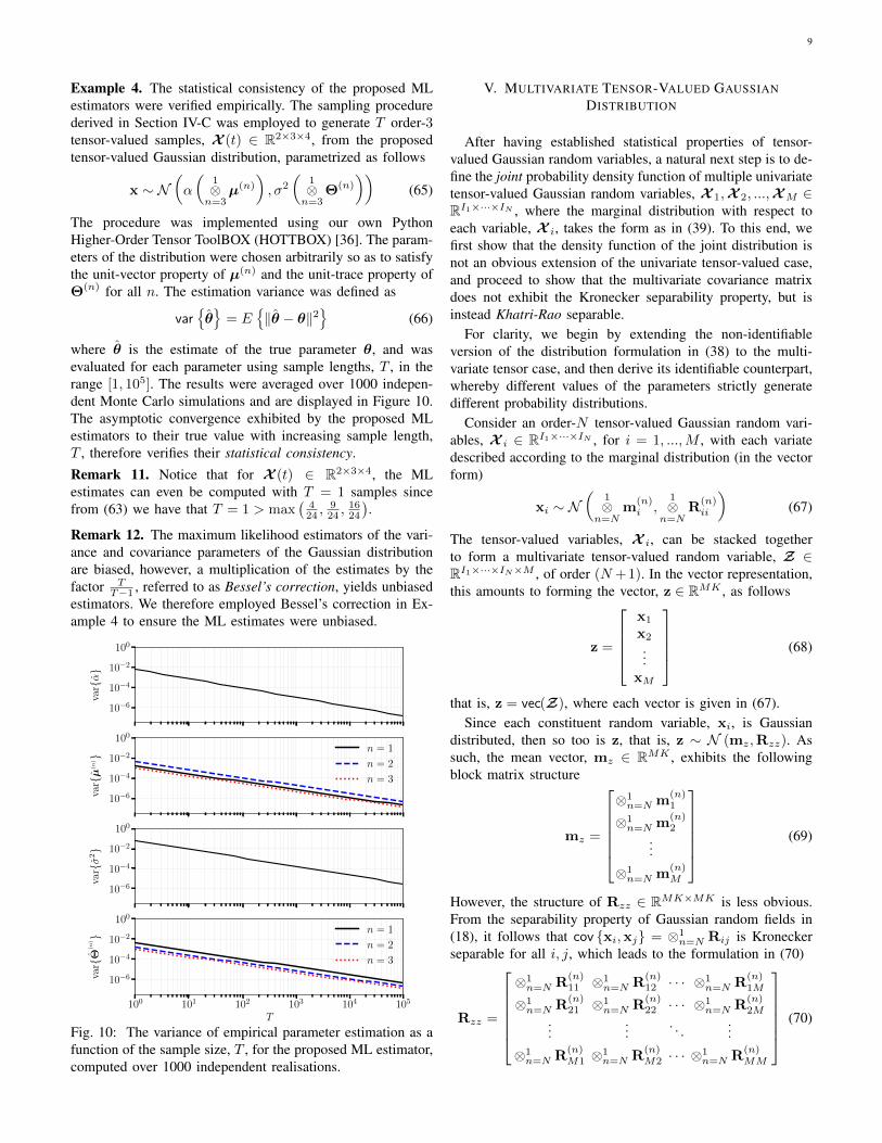
Example 4. The statistical consistency of the proposed MLestimators were verified empirically. The sampling procedurederived in Section IV-C was employed to generate T order-3tensor-valued samples, X (t) ∈ R2×3×4, from the proposedtensor-valued Gaussian distribution, parametrized as follows
x ∼ NÅα
Å1⊗n=3
µ(n)
ã, σ2
Å1⊗n=3
Θ(n)
ãã(65)
The procedure was implemented using our own PythonHigher-Order Tensor ToolBOX (HOTTBOX) [36]. The param-eters of the distribution were chosen arbitrarily so as to satisfythe unit-vector property of µ(n) and the unit-trace property ofΘ(n) for all n. The estimation variance was defined as
var¶θ©= E
¶‖θ − θ‖2
©(66)
where θ is the estimate of the true parameter θ, and wasevaluated for each parameter using sample lengths, T , in therange [1, 105]. The results were averaged over 1000 indepen-dent Monte Carlo simulations and are displayed in Figure 10.The asymptotic convergence exhibited by the proposed MLestimators to their true value with increasing sample length,T , therefore verifies their statistical consistency.Remark 11. Notice that for X (t) ∈ R2×3×4, the MLestimates can even be computed with T = 1 samples sincefrom (63) we have that T = 1 > max
(424 ,
924 ,
1624
).
Remark 12. The maximum likelihood estimators of the vari-ance and covariance parameters of the Gaussian distributionare biased, however, a multiplication of the estimates by thefactor T
T−1 , referred to as Bessel’s correction, yields unbiasedestimators. We therefore employed Bessel’s correction in Ex-ample 4 to ensure the ML estimates were unbiased.
10−6
10−4
10−2
100
var{α}
10−6
10−4
10−2
100
var{µ
(n)} n = 1
n = 2
n = 3
10−6
10−4
10−2
100
var{σ
2}
100 101 102 103 104 105
T
10−6
10−4
10−2
100
var{
Θ(n
)} n = 1
n = 2
n = 3
Fig. 10: The variance of empirical parameter estimation as afunction of the sample size, T , for the proposed ML estimator,computed over 1000 independent realisations.
V. MULTIVARIATE TENSOR-VALUED GAUSSIANDISTRIBUTION
After having established statistical properties of tensor-valued Gaussian random variables, a natural next step is to de-fine the joint probability density function of multiple univariatetensor-valued Gaussian random variables, X 1,X 2, ...,XM ∈RI1×···×IN , where the marginal distribution with respect toeach variable, X i, takes the form as in (39). To this end, wefirst show that the density function of the joint distribution isnot an obvious extension of the univariate tensor-valued case,and proceed to show that the multivariate covariance matrixdoes not exhibit the Kronecker separability property, but isinstead Khatri-Rao separable.
For clarity, we begin by extending the non-identifiableversion of the distribution formulation in (38) to the multi-variate tensor case, and then derive its identifiable counterpart,whereby different values of the parameters strictly generatedifferent probability distributions.
Consider an order-N tensor-valued Gaussian random vari-ables, X i ∈ RI1×···×IN , for i = 1, ...,M , with each variatedescribed according to the marginal distribution (in the vectorform)
xi ∼ NÅ
1⊗n=N
m(n)i ,
1⊗n=N
R(n)ii
ã(67)
The tensor-valued variables, X i, can be stacked togetherto form a multivariate tensor-valued random variable, Z ∈RI1×···×IN×M , of order (N +1). In the vector representation,this amounts to forming the vector, z ∈ RMK , as follows
z =
x1
x2
...xM
(68)
that is, z = vec(Z), where each vector is given in (67).Since each constituent random variable, xi, is Gaussian
distributed, then so too is z, that is, z ∼ N (mz,Rzz). Assuch, the mean vector, mz ∈ RMK , exhibits the followingblock matrix structure
mz =
⊗1n=N m
(n)1
⊗1n=N m
(n)2
...
⊗1n=N m
(n)M
(69)
However, the structure of Rzz ∈ RMK×MK is less obvious.From the separability property of Gaussian random fields in(18), it follows that cov {xi,xj} = ⊗1
n=N Rij is Kroneckerseparable for all i, j, which leads to the formulation in (70)
Rzz =
⊗1n=N R
(n)11 ⊗1
n=N R(n)12 · · · ⊗1
n=N R(n)1M
⊗1n=N R
(n)21 ⊗1
n=N R(n)22 · · · ⊗1
n=N R(n)2M
......
. . ....
⊗1n=N R
(n)M1 ⊗1
n=N R(n)M2 · · · ⊗1
n=N R(n)MM
(70)

10
The multivariate tensor mean and covariance parameters in(69)-(70) can be equivalently expressed through the followingKhatri-Rao products
mz =1©∗
n=Nm(n)z , Rzz =
1©∗
n=NR(n)zz (71)
where m(n)z ∈ RMIn and R
(n)zz ∈ RMIn×MIn are respectively
the multivariate tensor mode-n mean and covariance parame-ters, defined as
m(n)z =
m
(n)1
m(n)2...
m(n)M
, R(n)zz =
R
(n)11 R
(n)12 · · · R
(n)1M
R(n)21 R
(n)22 · · · R
(n)2M
......
. . ....
R(n)M1 R
(n)M2 · · · R
(n)MM
(72)
Therefore, the vector representation, z ∈ RMK , is distributedaccording to
z ∼ NÅ
1©∗
n=Nm(n)z ,
1©∗
n=NR(n)zz
ã(73)
which asserts that the joint probability density function of thetensor-valued random variables X 1, ...,XM is given by
p(Z) =exp
[− 1
2 (z−mz)TÄ©∗ 1n=N R
(n)zz
ä−1(z−mz)
](2π)
MK2 det
12
Ä©∗ 1n=N R
(n)zz
ä(74)
where mz =Ä©∗ 1n=N m
(n)z
ä.
With the above derived properties of the multivariate tensor-valued distribution we obtain the following result.
Proposition 1. The multivariate tensor-valued random vari-able, z ∈ RMK , is said to exhibit a Khatri-Rao separablestatistics if and only if the following properties hold
E {z} = 1©∗
n=Nm(n)z (75)
cov {z} = 1©∗
n=NR(n)zz (76)
cov{Z(n)
}=
(N�i=1i6=n
ptrÄR(i)zz
ä)©∗ R(n)
zz (77)
where � denotes the Hadamard (element-wise) product. Withreference to the constituent tensor-valued random variables,the separability properties in (76)-(77) reduce to the following
cov {xi,xj} =1⊗n=N
R(n)ij (78)
cov{Xi(n),Xj(n)
}=
(N∏k=1k 6=n
trÄR
(k)ij
ä)R
(n)ij (79)
Remark 13. As shown in Section IV-A for the univariatetensor-valued case, the proposed multivariate tensor-valuedGaussian distribution described by the second-order statisticsin (78)-(79) is non-identifiable, whereby different values of theparameters may generate equivalent probability distributions,and therefore the parameters cannot be estimated analytically.
A. The statistically identifiable formulation
Following the establishment of the analytical framework fortensor-valued probability distribution in Section IV, we nowintroduce the identifiable counterpart of the proposed multi-variate tensor-valued distribution in (74), whereby differentvalues of the parameters strictly generate different probabilitydistributions, based on the following rationale.
The expected inner product between pairwise tensor-valuedrandom variables, X i and X j , is invariant to the data repre-sentation, that is
E {〈X i,X j〉} = E {〈xi,xj〉} = E{〈Xi(n),Xj(n)〉
}(80)
for all n, and for both the direct data format and any vectoror matrix tensor unfolding. We can therefore dissociate theexpected inner product scale, σij = E {〈X i,X j〉}, fromthe mode-n covariance matrices, R
(n)ij , by introducing the
parameter Θ(n)ij ∈ RIn×In to yieldÅ
1⊗n=N
R(n)ij
ã= σij
Å1⊗n=N
Θ(n)ij
ã(81)
where
σij = tr
Å1⊗n=N
R(n)ij
ã(82)
To obtain an identifiable parametrization we must also imposethe unit-trace property on the introduced matrices, that is,trÄΘ
(n)ij
ä= 1, ∀n, so as to resolve the scaling ambiguity
arising in Kronecker products described in Section IV-A.
Remark 14. Intuitively, Θ(n)ij can also be viewed as the
covariance density at the n-th mode, whereby it describes thepercentage of the total covariance, σij , assigned to each pairof mode-n fibers. Moreover, the unit-trace condition satisfiesthe definition in (82).
Furthermore, the separability property of the mean of X i inthe identifiable formulation, given by Mi = αi
Ä◦Nn=1 µ
(n)i
ä,
also applies herein.By jointly considering the parameters, αi, µ
(n)i , σij and
Θ(n)ij , for all i, j = 1, ...,M and n = 1, ..., N , we can now
form the matrices
αz =
α1
α2
...αM
∈ RM (83)
µ(n)z =
µ
(n)1
µ(n)2...
µ(n)M
∈ RMIn (84)
Σzz =
σ21 σ12 · · · σ1M
σ21 σ22 · · · σ2M
......
. . ....
σM1 σM2 · · · σ2M
∈ RM×M (85)

11
Θ(n)zz =
Θ
(n)11 Θ
(n)12 · · · Θ
(n)1M
Θ(n)21 Θ
(n)22 · · · Θ
(n)2M
......
. . ....
Θ(n)M1 Θ
(n)M2 · · · Θ
(n)MM
∈ RMIn×MIn
(86)
so that the proposed distribution is formulated as follows
z ∼ NÅÅ
αz1©∗
n=Nµ(n)z
ã,
ÅΣzz
1©∗
n=NΘ(n)zz
ãã(87)
The multivariate tensor probability density function then be-comes
p(z) =exp
[− 1
2 (z−mz)TÄΣzz©∗ 1n=N Θ(n)
zz
ä−1(z−mz)
](2π)
K2 det
12
ÄΣzz©∗ 1n=N Θ(n)
zz
ä(88)
where mz =Äαz ©∗ 1n=N µ
(n)z
ä.
Remark 15. For M = 1, the proposed multivariate tensor-valued probability distribution in (88) reduces to the univariatetensor-valued probability distribution in (51).
With the proposed identifiable formulation, the Khatri-Raoseparability properties of multivariate tensor-valued randomvariable, z ∈ RMK , are given by
E {z} =Åαz
1©∗
n=Nµ(n)z
ã(89)
cov {z} =Å
Σzz
1©∗
n=NΘ(n)zz
ã(90)
cov{Z(n)
}=ÄΣzz ©∗ Θ(n)
zz
ä(91)
With reference to the constituent tensor-valued random vari-ables, the Khatri-Rao separability properties of the covariancesimplify to
E {xi} = αi
Å1⊗n=N
µ(n)i
ã(92)
cov {xi,xj} = σij
Å1⊗n=N
Θ(n)ij
ã(93)
cov{Xi(n),Xj(n)
}= σijΘ
(n)ij (94)
B. Maximum likelihood tensor-valued estimator
Since multivariate tensor-valued Gaussian probability dis-tribution is a natural extension of the univariate tensor-valuedcase, this gives us the opportunity to employ the proposedrelationships in (93)-(94) to obtain the ML estimators
σij =1
T
T−1∑t=0
sTi (t)sj(t) (95)
Θ(n)ij =
1
Tσij
T−1∑t=0
Si(n)(t)STj(n)(t) (96)
where σ2i ≡ σii. Furthermore, the ML estimation procedure
for determining αi and {µ(n)i }Nn=1 is equivalent to that for
univariate tensor-valued variables, that is, they are obtainedfrom the rank-1 multilinear SVD of the sample mean tensor1T
∑T−1t=0 X i(t).
VI. APPLICATIONS TO ATMOSPHERIC CLIMATE ANALYSIS
In this section, we demonstrate the ability of the proposedprobabilistic model in (51) to statistically characterise atmo-spheric climate data. We modelled the ECMWF ReAnalysis(ERA5) dataset [37], which provides global estimates ofatmospheric, land and oceanic climate variables in time, as atensor-valued Gaussian random variable. We considered dailytemperature measurements, each recorded at 00:00 GMT, ata horizontal resolution of 31 km for 20 altitude levels withinthe troposphere, ranging from the surface up to an altitude of11 km. Each sample at a time instant t naturally takes the formof an order-3 tensor, X (t) ∈ RI1×I2×I3 , where I1 = 721,I2 = 1440 and I3 = 20 denote respectively the number oflatitude, longitude, and altitude grid points. We consideredsamples ranging in the period 2019-10-01 to 2019-10-31, i.e.T = 31 daily tensor-valued samples, thereby forming of anorder-4 tensor, D ∈ RI1×I2×I3×T , as illustrated in Figure 11.
Altitudes
Longitudes
Latitu
des
Samples
1
Fig. 11: Construction of the order-4 data tensor. Each sample,X (t) ∈ RI1×I2×I3 , consists of temperature measurements inthe longitude × latitude × altitude space at a time instant t.
The statistical analysis was implemented using our ownPython Higher-Order Tensor ToolBOX (HOTTBOX) [36].The sample mean, 1
T
∑Tt=1 X (t), and its associated mean
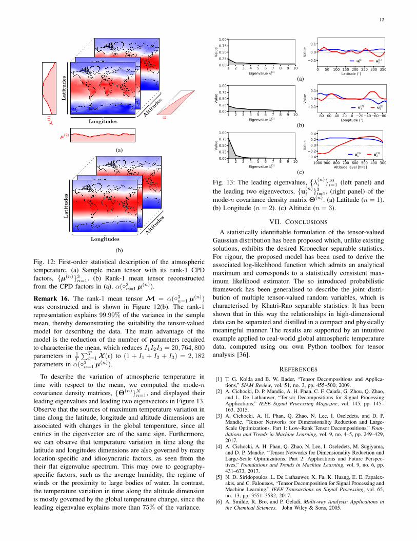
parameters, α and {µ(n)}3n=1 in (51), were evaluated andare shown in Figure 12(a). Observe that the mode-1 CPDfactor, µ(1), conveys the expected variation of temperature inthe latitude dimension, whereby the maximum temperature isobserved at the equator. The mode-2 CPD factor associatedwith the variation of temperature in the longitude dimension,µ(2), conveys the diurnal temperature variation, that is, thedifference in temperature between regions in day and nighttime. Similarly, the mode-3 CPD factor, µ(3), depicts theexpected decrease in atmospheric temperature with an increasein altitude, which arises from the radiation and convectionbehaviours typically observed in the troposphere.
12
Altitudes
Longitudes
Latitu
des
µ(1)
µ(2)
µ(3)
1
(a)
Altitudes
Longitudes
Latitu
des
1
(b)
Fig. 12: First-order statistical description of the atmospherictemperature. (a) Sample mean tensor with its rank-1 CPDfactors, {µ(n)}3n=1. (b) Rank-1 mean tensor reconstructedfrom the CPD factors in (a), α(◦3n=1 µ
(n)).
Remark 16. The rank-1 mean tensor M = α(◦3n=1 µ(n))
was constructed and is shown in Figure 12(b). The rank-1representation explains 99.99% of the variance in the samplemean, thereby demonstrating the suitability the tensor-valuedmodel for describing the data. The main advantage of themodel is the reduction of the number of parameters requiredto characterise the mean, which reduces I1I2I3 = 20, 764, 800parameters in 1
T
∑Tt=1 X (t) to (1 + I1 + I2 + I3) = 2, 182
parameters in α(◦3n=1 µ(n)).
To describe the variation of atmospheric temperature intime with respect to the mean, we computed the mode-ncovariance density matrices, {Θ(n)}Nn=1, and displayed theirleading eigenvalues and leading two eigenvectors in Figure 13.Observe that the sources of maximum temperature variation intime along the latitude, longitude and altitude dimensions areassociated with changes in the global temperature, since allentries in the eigenvector are of the same sign. Furthermore,we can observe that temperature variation in time along thelatitude and longitudes dimensions are also governed by manylocation-specific and idiosyncratic factors, as seen from thetheir flat eigenvalue spectrum. This may owe to geography-specific factors, such as the average humidity, the regime ofwinds or the proximity to large bodies of water. In contrast,the temperature variation in time along the altitude dimensionis mostly governed by the global temperature change, since theleading eigenvalue explains more than 75% of the variance.
1 2 3 4 5 6 7 8 9 10Eigenvalue (1)
i
0.000.250.500.751.00
Valu
e
0 50 100 150 200 250 300 350Latitude ( )
0.1
0.0
0.1
Valu
e
u(1)1 u(1)
2
(a)
1 2 3 4 5 6 7 8 9 10Eigenvalue (2)
i
0.000.250.500.751.00
Valu
e
80604020020406080Longitude ( )
0.1
0.0
0.1
Valu
e
u(2)1 u(2)
2
(b)
1 2 3 4 5 6 7 8 9 10Eigenvalue (3)
i
0.000.250.500.751.00
Valu
e
3004005006007008009001000Altitude level [hPa]
0.40.20.00.20.4
Valu
e
u(3)1 u(3)
2
(c)
Fig. 13: The leading eigenvalues, {λ(n)i }10i=1 (left panel) andthe leading two eigenvectors, {u(n)
i }3i=1, (right panel) of themode-n covariance density matrix Θ(n). (a) Latitude (n = 1).(b) Longitude (n = 2). (c) Altitude (n = 3).
VII. CONCLUSIONS
A statistically identifiable formulation of the tensor-valuedGaussian distribution has been proposed which, unlike existingsolutions, exhibits the desired Kronecker separable statistics.For rigour, the proposed model has been used to derive theassociated log-likelihood function which admits an analyticalmaximum and corresponds to a statistically consistent max-imum likelihood estimator. The so introduced probabilisticframework has been generalised to describe the joint distri-bution of multiple tensor-valued random variables, which ischaracterised by Khatri-Rao separable statistics. It has beenshown that in this way the relationships in high-dimensionaldata can be separated and distilled in a compact and physicallymeaningful manner. The results are supported by an intuitiveexample applied to real-world global atmospheric temperaturedata, computed using our own Python toolbox for tensoranalysis [36].
REFERENCES
[1] T. G. Kolda and B. W. Bader, “Tensor Decompositions and Applica-tions,” SIAM Review, vol. 51, no. 3, pp. 455–500, 2009.
[2] A. Cichocki, D. P. Mandic, A. H. Phan, C. F. Caiafa, G. Zhou, Q. Zhao,and L. De Lathauwer, “Tensor Decompositions for Signal ProcessingApplications,” IEEE Signal Processing Magazine, vol. 145, pp. 145–163, 2015.
[3] A. Cichocki, A. H. Phan, Q. Zhao, N. Lee, I. Oseledets, and D. P.Mandic, “Tensor Networks for Dimensionality Reduction and Large-Scale Optimizations. Part 1: Low–Rank Tensor Decompositions,” Foun-dations and Trends in Machine Learning, vol. 9, no. 4–5, pp. 249–429,2017.
[4] A. Cichocki, A. H. Phan, Q. Zhao, N. Lee, I. Oseledets, M. Sugiyama,and D. P. Mandic, “Tensor Networks for Dimensionality Reduction andLarge-Scale Optimizations. Part 2: Applications and Future Perspec-tives,” Foundations and Trends in Machine Learning, vol. 9, no. 6, pp.431–673, 2017.
[5] N. D. Siridopoulos, L. De Lathauwer, X. Fu, K. Huang, E. E. Papalex-akis, and C. Faloutsos, “Tensor Decomposition for Signal Processing andMachine Learning,” IEEE Transactions on Signal Processing, vol. 65,no. 13, pp. 3551–3582, 2017.
[6] A. Smilde, R. Bro, and P. Geladi, Multi-way Analysis: Applications inthe Chemical Sciences. John Wiley & Sons, 2005.

13
[7] S. Klus, P. Gelß, S. Peitz, and Schutte, “Tensor-Based Dynamic ModeDecomposition,” Nonlinearity, vol. 31, no. 7, pp. 3359–3380, 2018.
[8] C. Liu and K. Koike, “Extending Multivariate Space-Time Geostatisticsfor Environmental Data Analysis,” Mathematical Geology, vol. 39, pp.289–305, 2007.
[9] P. J. Basser and S. Pajevic, “A Normal Distribution for Tensor-ValuedRandom Variables: Applications to Diffusion Tensor MRI,” IEEE Trans-actions on Medical Imaging, vol. 22, no. 7, pp. 785–794, 2003.
[10] H. A. Kiers and I. V. Mechelen, “Three-Way Component Analysis:Principles and Illustrative Application,” Psychological Methods, vol. 6,no. 1, pp. 84–110, 2001.
[11] C. Soize, “Tensor-Valued Random Fields for Meso-Scale StochasticModel of Anisotropic Elastic Microstructure and Probabilistic Analysisof Representative Volume Element Size,” Probabilistic EngineeringMechanics, vol. 23, pp. 307–323, 2007.
[12] N. D. Siridopoulos, G. Giannakis, and R. Bro, “Blind PARAFACReceivers for DS-CDMA Systems,” IEEE Transactions on Signal Pro-cessing, vol. 48, no. 3, pp. 810–823, 2000.
[13] L. Spyrou, M. Parra, and J. Escudero, “Complex Tensor factorisationwith PARAFAC2 for the Estimation of Brain Connectivity from theEEG,” IEEE Transactions on Neural Systems and Rehabilitation Engi-neering, vol. 27, no. 1, pp. 1–12, 2018.
[14] W. Chu and Z. Ghahramani, “Probabilistic Models for IncompleteMulti-Dimensional Arrays,” Journal of Machine Learning Research -Proceedings Track, vol. 5, pp. 89–96, 2009.
[15] P. D. Hoff, “Separable Covariance Arrays via the Tucker Product, withApplications to Multivariate Relational Data,” Bayesian Analysis, vol. 6,no. 2, pp. 179–196, 2011.
[16] M. Ohlson, M. R. Ahmad, and D. von Rosen, “The Multilinear Nor-mal Distribution: Introduction and Some Basic Properties,” Journal ofMultivariate Analysis, vol. 113, pp. 37–47, 2013.
[17] A. P. Dawid, “Some Matrix-Variate Distribution Theory: Notional Con-siderations and a Bayesian Application,” Boimetrika, vol. 68, no. 1, pp.265–274, 1981.
[18] J. M. Quintana and M. West, “Time Series Analysis of CompositionalData,” in Bayesian Statistics 3, J. M. Bernardo, M. H. DeGroot, D. V.Lindley, and A. F. M. Smith, Eds. Oxford University Press, 1988.
[19] A. K. Gupta and D. K. Nagar, Matrix Variate Distributions. BocaRaton, Florida: Chapman & Hall/CRC, 2000.
[20] Z. Xu, F. Yan, and Y. Qi, “Infinite Tucker decomposition: NonparametricBayesian Models for Multiway Data Analysis,” In Proceedings of the29th International Conference on Machine Learning (ICML), pp. 1675–1682, 2012.
[21] P. Dutilleul, “The MLE Algorithm for the Matrix Normal Distribution,”Journal of Statistical Computation and Simulation, vol. 64, pp. 105–123,1999.
[22] A. M. Manceur and P. Dutilleul, “Maximum Likelihood Estimation forthe Tensor Normal Distribution: Algorithm, Minimum Sample Size, andEmpirical Bias and Dispersion,” Journal of Computational and AppliedMathematics, vol. 239, pp. 37–49, 2013.
[23] J. Nzabanita, D. von Rosen, and M. Singull, “Maximum LikelihoodEstimation in the Tensor Normal Model with a Structured Mean,”Linkoping University Electronic Press, LiTH-MAT-R-2015/08-SE, 2015.
[24] K. Werner, M. Jansson, and P. Stoica, “On Estimation of CovarianceMatrices with Kronecker Product Structure,” IEEE Transactions onSignal Processing, vol. 56, no. 2, pp. 478–491, 2008.
[25] N. A. Weiss, P. T. Holmes, and M. Hardy, A Course in Probability.Pearson Addison Wesley, 2005.
[26] P. Tseng, “Convergence of a Block Coordinate Descent Method forNondifferentiable Minimization,” Journal of Optimization Theory andApplications, vol. 109, no. 3, pp. 475–494, 2001.
[27] A. Uschmajew, “Local Convergence of the Alternating Least SquaresAlgorithm for Canonical Tensor Approximation,” SIAM Journal onMatrix Analysis and Applications, vol. 33, no. 2, pp. 639–652, 2012.
[28] T. Rohwedder and A. Uschmajew, “On Local Convergence of Alternat-ing Schemes for Optimization of Convex Problems in the Tensor TrainFormat,” SIAM Journal on Numerical Analysis, vol. 51, no. 2, pp. 1134–1162, 2013.
[29] M. Rupp and S. Schwarz, “A Tensor LMS Algorithm,” In Proceedingsof the International Conference on Acoustics, Speech and Signal Pro-cessing (ICASSP), pp. 3347–3351, 2015.
[30] W. K. Newey and D. McFadden, “Large Sample Estimation and Hy-pothesis Testing,” Handbook of Econometrics, vol. 4, pp. 2111–2245,1994.
[31] D. Gerards and P. D. Hoff, “Equivariant Minimax Dominators of theMLE in the Array Normal Model,” Journal of Multivariate Analysis,vol. 137, pp. 32–49, 2015.
[32] L. De Lathauwer, B. D. Moor, and J. Vandewalle, “A MultilinearSingular Value Decomposition,” SIAM Journal on Matrix Analysis andApplications, vol. 21, no. 4, pp. 1253–1278, 2000.
[33] C. F. Van Loan, “Structured Matrix Problems from Tensors,” in Ex-ploiting Hidden Structures in Matrix Computations: Algorithms andApplications, M. Benzi and V. Simoncini, Eds. Cetraro: Springer, 2016,pp. 1–63.
[34] K. M. Abadir and J. R. Magnus, Matrix Algebra. Cambridge UniversityPress, 2005.
[35] V. S. Huzurbazar, “The Likelihood Equations, Consistency and theMaxima of the Likelihood Equation,” Annals of Eugenics, vol. 14, no. 1,pp. 185–200, 1947.
[36] I. Kisil, B. Scalzo Dees, A. Moniri, G. G. Calvi, and D. P. Mandic,“HOTTBOX: Higher Order Tensor ToolBOX,” https://hottbox.github.io.
[37] ECMWF Reanalysis (ERA5). [Online]. Available: https://www.ecmwf.int/en/forecasts/datasets/reanalysis-datasets/era5
PLACEPHOTOHERE
Bruno Scalzo Dees received the M.Eng. degree inaeronautical engineering from Imperial College Lon-don, U.K. He is currently working toward the Ph.D.degree at the Department of Electrical Engineeringat the same institution. His research interests includestatistical signal processing, maximum entropy mod-elling and tensor-valued random variables.
PLACEPHOTOHERE
Anh-Huy Phan (M’15) received the master’s degreefrom the Ho Chi Minh City University of Technol-ogy, Ho Chi Minh City, Vietnam, in 2005, and thePh.D. degree from the Kyushu Institute of Technol-ogy, Kitakyushu, Japan, in 2011. From October 2011to March 2018, he was a Research Scientist with theLaboratory for Advanced Brain Signal Processing,Brain Science Institute (BSI), RIKEN, Tokyo, Japan,where he was a Visiting Research Scientist withthe Toyota Collaboration Center, from April 2012to April 2015. Since May 2018, he has been an
Assistant Professor with the Center for Computational and Data-IntensiveScience and Engineering, Skoltech, Moscow, Russia. He is also a VisitingAssociate Professor with the Tokyo University of Agriculture and Technology(TUAT), Tokyo. He has authored three monographs. His research interestsinclude multilinear algebra, tensor computation, tensor networks, nonlinearsystem, blind source separation, and braincomputer interface.
Dr. Phan received best paper awards for articles in the IEEE SignalProcessing Magazine in 2018 and in the International Conference on NeuralInformation Processing in 2016, and the Outstanding Reviewer Award formaintaining the prestige of the IEEE International Conference on Acoustics,Speech and Signal Processing 2019.
PLACEPHOTOHERE
Danilo P. Mandic (M’99-SM’03-F’12) received thePh.D. degree in nonlinear adaptive signal processingfrom Imperial College London, U.K., in 1999.
He has been a Guest Professor with KatholiekeUniversiteit Leuven, Leuven, Belgium, the TokyoUniversity of Agriculture and Technology, Tokyo,Japan, Westminster University, London, and a Fron-tier Researcher with RIKEN, Wako, Japan. He is cur-rently a Professor of signal processing with ImperialCollege London, where he is involved in nonlinearadaptive signal processing and nonlinear dynamics.
He is also the Deputy Director of the Financial Signal Processing Laboratory,Imperial College London. He has two research monographs Recurrent NeuralNetworks for Prediction: Learning Algorithms, Architectures and Stability(West Sussex, U.K.: Wiley, 2001) and Complex Valued Nonlinear AdaptiveFilters: Noncircularity, Widely Linear and Neural Models (West Sussex, U.K.:Wiley, 2009), an edited book Signal Processing Techniques for KnowledgeExtraction and Information Fusion (New York, NY, USA: Springer, 2008),and more than 200 publications on signal and image processing.
Prof. Mandic has been a member of the IEEE Technical Committee onSignal Processing Theory and Methods. He has produced award winningpapers and products resulting from his collaboration with the industry. Hehas been an Associate Editor of the IEEE Signal Processing Magazine,the IEEE TRANSACTIONS ON CIRCUITS AND SYSTEMS II, the IEEETRANSACTIONS ON SIGNAL PROCESSING, and the IEEE TRANSACTIONSON NEURAL NETWORKS.