a study of 3d finite element modeling method for stagger ... · a study of 3d finite element...

Wang et al. / J Zhejiang Univ-Sci A (Appl Phys & Eng) 2016 17(8):646-666 646

A study of 3D finite element modeling method for

stagger spinning of thin-walled tube*

Jin WANG†1, Ting GE1,2, Guo-dong LU1, Fei LI1 (1State Key Laboratory of Fluid Power and Mechatronic Systems, Zhejiang University, Hangzhou 310027, China)

(2Jiangsu Posts & Telecommunications Planning and Designing Institute Co., Ltd., Nanjing 210000, China) †E-mail: [email protected]

Received June 17, 2015; Revision accepted Nov. 2, 2015; Crosschecked July 24, 2016

Abstract: A modified 3D finite element (3D-FE) model is developed under the FE software environment of LS-DYNA based on characteristics of stagger spinning process and actual production conditions. Several important characteristics of the model are proposed, including full model, hexahedral element, speed boundary mode, full simulation, double-precision mode, and no-interference. Modeling procedures and key technologies are compared and summarized: speed mode is superior to displace-ment mode in simulation accuracy and stability; time truncation is an undesirable option for analysis of the distribution trend of time-history parameters to guarantee that the data has reached the stable state; double-precision mode is more suitable for stagger spinning simulation, as truncation error has obvious effects on the accuracy of results; interference phenomenon can lead to ob-vious oscillation and mutation simulation results and influence the reliability of simulation significantly. Then, based on the modified model, some improvements of current reported results of roller intervals have been made, which lead to higher accuracy and reliability in the simulation.

Key words: Stagger spinning, 3D finite element (3D-FE) modeling, Roller interval, Thin-walled tube http://dx.doi.org/10.1631/jzus.A1500180 CLC number: TG306; TH162.1

1 Introduction

Tube spinning is an efficient and flexible process

for forming mental cylindrical hollow parts (Wong et al., 2003). Stagger spinning is a special tube spinning with complicated process. Three uniformly distrib-uted rollers in circumferential direction are staggered at certain intervals to complete multi-pass thinning in a single feed. Stagger spinning is a locally continuous forming process. With advantages such as multiple

constraints, higher shape and dimensional accuracy, lower consumption, and higher efficiency, it is more and more widely used in production of cylindrical parts with wall thickness reduction.

Surface quality (Fazeli and Ghoreishi, 2009), specific materials (Xu et al., 2005), and the geometric parameters (Fazeli and Ghoreishi, 2011) in the metal spinning process have been investigated using ex-periments and statistical principles. Experimental methods have high costs, restrictive conditions, de-tection limits, and many significant issues in the forming process. Finite element (FE) simulation is an effective method that is being more and more widely applied nowadays. It is widely used to study the in-fluence of the key parameters, such as roller path (Li et al., 2014), roller nose radius and release angle (Lexian and Dariani, 2009), displacement distribution (Li et al., 1998), and stress and strain distribution

Journal of Zhejiang University-SCIENCE A (Applied Physics & Engineering)

ISSN 1673-565X (Print); ISSN 1862-1775 (Online)

www.zju.edu.cn/jzus; www.springerlink.com

E-mail: [email protected]

* Project supported by the Zhejiang Provincial Natural Science Foundation of China (No. LY15E050003), the Specialized Research Fund for the Doctoral Program of Higher Education of China (No. 20120101130003), the Key Project of Science and Technology Program of Zhejiang Province (No. 2013C01135), and the Fundamental Research Funds for the Central Universities (No. 2015QNA4003), China

ORCID: Jin WANG, http://orcid.org/0000-0003-3106-021X © Zhejiang University and Springer-Verlag Berlin Heidelberg 2016


(Zoghi and Arezoodar, 2013). It has also proven to be a cost-effective method for defect observation (Hua et al., 2005) and parameter optimization (Essa and Hartley, 2010). Huang et al. (2008), Zhang et al. (2012), and Lexian and Dariani (2008) studied split spinning, large ellipsoidal heads spinning, and tube spinning using FE modeling, respectively.

There have also been some reports on FE mod-eling methods in the case of stagger spinning (Xue et al., 1997; Tan, 2009; Zhang et al., 2009; Ge, 2012; Li et al., 2013). In these simulations, some parameter setting conditions and simplified approaches of FE modeling were proposed to improve the computa-tional efficiency. The influence of roller intervals was studied based on these models. However, there are some disadvantages and inappropriate simplifications in those FE research models of stagger spinning, as discussed below.

1. Part model. Three rollers were assumed com-pletely symmetrical during the whole spinning pro-cess, and only one-third of the blank was adopted instead of the whole part (Xue et al., 1997). However, the roller intervals in stagger spinning have an obvi-ous influence on the circumferential balance and roller distribution.

2. Tetrahedron elements. Tetrahedron elements were adopted to disperse the blank (Tan, 2009; Zhang et al., 2009) and automatic meshing methods were used with limits such as large amounts as well as low accuracy and efficiency.

3. Displacement boundary. During the process of simulation, the roller system was fed in the dis-placement boundary as the blank and mandrel were fixed (Tan, 2009; Zhang et al., 2009; Li et al., 2013). It is inconsistent with the actual production condition. Besides, the passive rotation of rollers and blank was ignored.

4. Single-precision mode. Default single- precision calculation was applied, and the influence of truncation error was not given enough attention (Li et al., 2013).

5. Time truncation. Artificially shortened ter-mination time was used to break off the simulation for time-history result extraction as the long simulation time for the stagger spinning process (Li et al., 2013).

6. Interference phenomenon. Because of the lack of effective means of prevention, interference phe-nomenon occurred frequently in the setting trials (Ge,

2012; Li et al., 2013) to investigate the influence of parameters, such as intervals, which had significant influence on the accuracy and stability of the results.

Though the above studies have made great con-tributions to the FE simulation analysis, the accuracy and reliability of the results were still questionable. According to the characteristics of stagger spinning, it is necessary to develop an improved FE model that is helpful in improving the study and understanding of the spinning process.

Roller interval has a significant influence on the stagger-spun products. Some researchers have also investigated this (Xia et al., 2012; Li et al., 2013). However, modeling problems, especially the inter-ference phenomenon, have very significant influence on the research results of roller intervals. The accu-racy and reliability of the results have been affected. It is also necessary to carry out research to improve upon the current results.

This paper aims at developing a modified 3D-FE model of stagger spinning to improve the aforemen-tioned defects. The model has characteristics of full model, hexahedral element, speed boundary mode, full simulation, double-precision mode, and non- interference. Influences of problems, including the precision mode, time truncation, boundary mode, and interference phenomenon, were investigated. 2 Establishment of 3D-FE model of stagger spinning

2.1 Basic parameter setting

1. Model extraction. Based on the platform of LS-DYNA, a 3D-FE model of stagger spinning, which includes the blank, mandrel, and three cir-cumferentially uniform rollers, is established, which considers the comprehensive problems existing in previous studies, as shown in Fig. 1. There are four available types of rollers in stagger spinning, as shown in Fig. 2.

The most widely used double-cone roller (Fig. 2c) is adopted in this study. Considering the thickness of the shell element, an appropriate gap is set between the mandrel and blank (Zhao and Li, 2008), as shown in Table 1. Table 2 shows the detailed parameters for the 3D-FE model (Cheng et al., 2011; Li et al., 2013; Ge et al., 2015). The thinning ratio of


the wall thickness of this model is set as 30%, ac-cording to the data reported by Zhang et al. (2009).

2. Grid type and generation. According to the deformation characteristic of each component, blank is set as a deformable solid part. During the spinning process, the mandrel, where there is no requirement to analyze its force, just plays the role of supporting the deformation process of the blank. However, the ex-traction of the roller force is necessary for further analysis. Thus, the mandrel and three rollers are

defined as the discrete rigid part and analytical rigid part, respectively (Huang et al., 2008), which are meshed with quadrilateral shell elements. It has been proved that the roller radius has a significant influ-ence on the tube spinning process, while the roller intervals in stagger spinning make the characteristics of circumferential balance and roller distribution different from normal tube spinning (Zhang et al., 2009; Ge et al., 2015). Thus, in the process of mod-eling, the roller radius is considered and the whole model is adopted.

Based on the forming characteristics and spin-ning conditions of the blank, the hexahedral elements, rotating from quadrilateral surface elements, are used to disperse the blank. Tetrahedral elements (Gadala and Wang, 1999; Zhang et al., 2009) were used in previous studies, which are not suitable for stagger spinning, with limitations such as large amounts as well as low accuracy and efficiency (Ge, 2012). Considering that the roller and mandrel are set as rigid parts without deformation, three rollers and mandrel are meshed with quadrilateral surface elements, as shown in Fig. 3.

3. Material properties. The blank is the only de-formable part in stagger spinning. The segment-line plastic model has been applied to describe the mate-rial. Here we adopt the explicit FE solution to analyze the forming process. The von Mises yielding

Table 1 Selection of the gap between the mandrel and the inner diameter of the blank

Inner diameter (mm) Gap and inner diameter ratio (%)

<100 0.25

100–200 0.20

200–400 0.15

400–700 0.10

700–1200 0.08

>1200 0.06

Roller Mandrel

Rotate

Blank

(a) (b) (c)

Fig. 3 Grid type and generation of the model (a) Hexahedral elements of reduced quadratic integral witheight nodes; (b) Quadrilateral surface elements of the roller;(c) Quadrilateral surface elements of the mandrel

Table 2 Detailed parameters for the geometric model and the process conditions (Ge et al., 2015)

Blank Normal double cone rollers Spinning conditions

Wall thickness

(mm)

Inner diameter

(mm)

Cylindrical part length

(mm)

Top radius, ρ

(mm)

Diameter (mm)

Smoothing angle, β (°)

Attack angle, α

(°)

Feed rate (mm/r)

Thickness reduction

(%)

Mandrel speed

(r/min)

2 130 100 5 270 10 28 0.8 30 200

Rr

(a) (b) (c) (d)

Fig. 2 Types of rollers that are used in stagger spinning(a) Round roller; (b) Single-cone roller; (c) Double-cone roller;(d) Stair roller. Rr: fillet radius; α: attack angle; β: smoothing angle; γ: the second attack angle; ρ: top radius

(a) (b)

Fig. 1 3D-FE model of stagger spinning (a) Axial view of the model; (b) Front view of the model


criterion and isotropic hardening have been used to model the material plastic response. Stress–strain curve of mild steel (DC01) has been obtained by tensile tests, as shown in Fig. 4. The true stress–strain curve is applied to the model based on the engineering curve obtained from experiments. Some elastic properties are as follows: mass density (7860 kg/m3), Young’s modulus (210 GPa), and Poisson’s ratio (0.3). Li et al. (2013) and Ge et al. (2015) set the friction coefficient of 0.2 and 0.05 between blank and man-drel and between blank and rollers, respectively. The friction coefficient between the blank and roller is lower, as the roller rotates passively along its own axis in the local coordinate. The Coulomb friction coefficients are set in the contact pairs (Li et al., 2013; Ge et al., 2015), which are defined in hypermesh. As the simulation parameters are basically similar, the value is 0.2 (between mandrel and blank) and 0.05 (between rollers and blank) according to data reported by Li et al. (2013) and Ge et al. (2015).

4. Boundary condition. Speed feeding mode and

displacement feeding mode are two different bound-ary conditions. As shown in Fig. 5a, similar to actual situation, the feeds of the mandrel and blank are driven by a constant torque or speed in speeding feeding mode, while it is the roller feed at a constant speed in axial direction. However, in the displacement feeding mode, displacement transformations are used to apply the motions of mandrel and blank to rollers to realize the equivalent movement, as shown in Fig. 5b.

The envelope of displacement indicates the trace of three rollers. In stagger spinning, the equivalent traces of rollers are in spiral shape; this kind of dis-placement feeding is called the spiral feeding mode.

Both feeding modes are considered as acceptable. The widely used displacement feeding mode of stagger spinning, which is inconsistent with the actual pro-duction condition and with limits of low accuracy and efficiency, is replaced with the speed feeding mode (Mohebbi and Akbarzadeh, 2010), as shown in Fig. 5. Detailed explanations will be offered later.

As shown in Fig. 5a, the blank rotates with the

mandrel, while the rollers feed directly and rotate passively around the center of mass. The circles with different sizes in the center reflect the different pas-sive rotational speeds of three rollers.

To realize the speed boundary mode and passive rotation of rollers, each component of the model is assigned with a reference point and local Cartesian coordinate system, as shown in Fig. 6. Although LS-DYNA does not support the cylindrical coordinate system in the calculation process, the rotation and the straight feed of the roller can be easily realized due to the assigned reference point and the local Cartesian coordinate system.

Axial

Radial Circumferential

Fig. 6 Construction of the local coordinate system forsetting up the speed boundary mode

Fig. 5 Trace of points of three rollers under speed bound-ary (a) and displacement boundary (b) conditions

Roller 3

Roller 1

Roller 2

Roller 2

Roller 1

Roller 3

(a) (b)

Fig. 4 Stress–strain curve of DC01

True stress-strain curve

Engineering stress-strain curve

0 0.40.30.1 0.20

50

100

150

200

250

300

350

400

450

Str

ess

(MP

a)

Strain


The moment of inertia is necessary to realize the passive rotation of rollers, which can also be realized easily in the local coordinate system by setting the center of mass as the rotation center, without conver-sion to the global coordinate system.

5. Contact surface and pair. To ensure that the contact between each component and the relative position order are consistent with the actual working conditions during the whole simulation process, the contact surface of each component and the contact pairs are defined, which include the contact pair be-tween the master external surface of mandrel and slave inner surface of blank, and the contact pair between master external surfaces of rollers 1–3 and the slave external surface of blank, as shown in Fig. 7.

2.2 Specification of the basic models

1. Mechanical model. In the stagger spinning process, high displacement, stain, and load direction change with large deformation. There are three de-scription models under nonlinear conditions of sim-ulation: reference description model, correlation de-scription model, and space description model.

Compared with that of the correlation descrip-tion model, the grid of the space description model is fixed, which is suitable for dynamic analysis of the fluid to describe the transient flow of different nodes. The correlation description model and reference de-scription model are similar except that the real Cau-chy stress is used in each load incremental step of the former, which is more suitable to deal with nonlinear constitutive relation and track stress changes during deformation.

As the stagger spinning simulation process mainly focuses on the spatial displacement of specific nodes, the correlation description model is adopted

for the simulation analysis to deal with nonlinear constitutive relation, the true Cauchy stress, external load in free surface, and track stress changes during deformation. The virtual work equation (Zhao and Li, 2008) of a deformed blank is

B Sδ d δ d δ d ,ij ij i i i iV V S

e V f u V f u S (1)

where σij is the Cauchy stress component, δeij is the integrating unit of deformation tensor, fi

B is the component of the body force, fi

S is the component of the surface traction, δui is the integrating unit of in-cremental displacement, V is the volume of deformed body, and S is the surface of deformed body.

2. Friction model. Friction model is one of the boundary conditions that have significant influence on the simulation accuracy of the continuous local plastic forming process of stagger spinning. Both rolling and sliding frictions occur between each pairs during the process, while the contact pressure and areas change quickly.

In LS-DYNA, the direct constraint method is adopted to detect the contact condition, which applies contact force and motion constraints to the nodes in the contact area directly. Taking into account the forming characteristics of stagger spinning process, the nonlinear correction Coulomb friction model is applied.

rf n

c

2arctan ,

π

v

v

(2)

where σf is the tangential friction stress, μ is the fric-tion coefficient, σn is the contact normal stress, vr is the relative velocity, and vc is the critical relative velocity.

3. Contact model. In the stagger spinning pro-cess, plastic deformation occurs with the contact of the rollers. Appropriate contact model is important for simulating the spinning process realistically. LS- DYNA provides three types of contact surface pro-cessing algorithms (node-surface contact, one-side contact, and surface-surface contact). Considering the high nonlinearity of the simulation and impossibility to determine the contact direction during the spinning process in advance, the automatic contact model without manual intervention of the contact direction is adopted. The penetration range (dis) between

Fig. 7 Contact surfaces and pairs of stagger spinning

Master external surface of roller 3

Master external surface of roller 1

Master external surface of roller 2Master external

surface of mandrel

Slave inner surface of blank

Slave external surface of blank


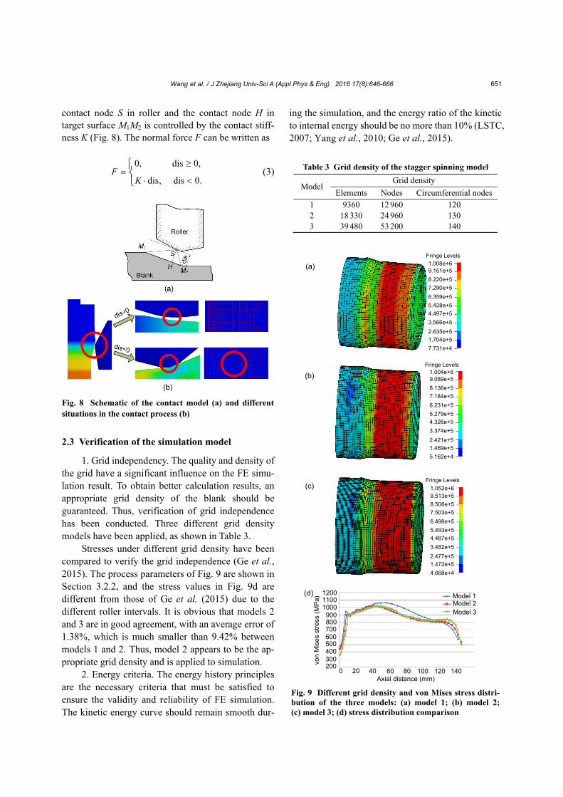
contact node S in roller and the contact node H in target surface M1M2 is controlled by the contact stiff-ness K (Fig. 8). The normal force F can be written as

0, dis 0,

dis, dis 0.F

K

(3)

2.3 Verification of the simulation model

1. Grid independency. The quality and density of the grid have a significant influence on the FE simu-lation result. To obtain better calculation results, an appropriate grid density of the blank should be guaranteed. Thus, verification of grid independence has been conducted. Three different grid density models have been applied, as shown in Table 3.

Stresses under different grid density have been compared to verify the grid independence (Ge et al., 2015). The process parameters of Fig. 9 are shown in Section 3.2.2, and the stress values in Fig. 9d are different from those of Ge et al. (2015) due to the different roller intervals. It is obvious that models 2 and 3 are in good agreement, with an average error of 1.38%, which is much smaller than 9.42% between models 1 and 2. Thus, model 2 appears to be the ap-propriate grid density and is applied to simulation.

2. Energy criteria. The energy history principles are the necessary criteria that must be satisfied to ensure the validity and reliability of FE simulation. The kinetic energy curve should remain smooth dur-

ing the simulation, and the energy ratio of the kinetic to internal energy should be no more than 10% (LSTC, 2007; Yang et al., 2010; Ge et al., 2015).

Table 3 Grid density of the stagger spinning model

ModelGrid density

Elements Nodes Circumferential nodes

1 9360 12 960 120 2 18 330 24 960 130 3 39 480 53 200 140

Fig. 9 Different grid density and von Mises stress distri-bution of the three models: (a) model 1; (b) model 2;(c) model 3; (d) stress distribution comparison

von

Mis

es s

tres

s(M

Pa

)

Axial distance (mm)0 20 40 60 80 100 120 140

200300400500600700800900

100011001200 Model 1

Model 2Model 3

Fringe Levels1.008e+69.151e+5

8.220e+5

7.290e+5

6.359e+5

5.428e+5

4.497e+5

3.566e+5

2.635e+5

1.704e+5

7.731e+4

Fringe Levels1.004e+69.089e+5

8.136e+5

7.184e+5

6.231e+5

5.279e+5

4.326e+5

3.374e+5

2.421e+5

1.469e+5

5.162e+4

Fringe Levels

1.052e+69.513e+5

8.508e+5

7.503e+5

6.498e+5

5.493e+5

4.487e+5

3.482e+5

2.477e+5

1.472e+5

4.668e+4

(a)

(b)

(c)

(d)

Fig. 8 Schematic of the contact model (a) and different situations in the contact process (b)


As shown in Fig. 10a, the kinetic energy rises quickly at the beginning because of the acceleration of the rollers and blank, and then it rises to the peak and appears almost steady because of the passive rotation of rollers. After about 20 s, the forming pro-cess attains stable spinning status and the kinetic energy changes little. It is clear that the kinetic energy satisfies the smoothness criterion.

Fig. 10b shows that the ratio of kinetic energy to internal energy decreases quickly after about 2 s of the acceleration period of the model and keeps much smaller than 10% from about 5 s due to the significant increase of internal energy. During the stable spinning status after about 20 s, the relative value keeps steady during the rest of the time, which fits well with the energy criterion.

The kinetic energy and ratio have similar varia-tion tendency with that of Ge et al. (2015) except the smaller value of kinetic energy, as most of the pa-rameter settings are similar. The value difference is caused by the different thinning ratios of the wall thickness due to the different roller intervals. To get a different kind of interference phenomenon, large reduction (about 45%) is applied in the model of Ge et al. (2015), but 30% (Zhang et al., 2009) is applied in this study. Smaller reductions will lead to both smaller kinetic and internal energy, and thus the en-ergy ratio tendency is similar to that of Ge et al. (2015).

3. Strain variation. Fig. 11 shows that the plastic strains of the internal and external elements have similar variation tendency with those of Hua et al.

CircumferentialRadicalAxial

0.4

0.2

0

-0.2

-0.4

Stroke of rollers (mm)

0 20 40 60 80 100

-0.4

-0.2

0

0.2

0.4

Pla

stic

str

ain


Pla

stic

str

ain

0 5 10 15 20 25

Circumferential

Radical

Axial

(c)(d)

0 5 10 15 20 25

-0.4

-0.2

0

0.2

0.4CircumferentialRadicalAxial



-0.4

-0.2

0

0.2

0.4

0 20 40 60 80 100

Pla

stic

str

ain

Pla

stic

str

ain

Radical

Circumferential

Axial

(b)(a)

Fig. 11 Deformation history by simulation (a) and Hua et al. (2005) (b) of internal surface element, and simulation (c) andHua et al. (2005) (d) of the external surface element

Ene

rgy

ratio

(%

)

0

20

40

60

80

100

0 255 10 15 20Time (s)

(b)

Fig. 10 Energy history verification: (a) kinetic energy; (b) energy ratio of kinetic and internal

0 5010 20 30 401

2

3

4

5

6

Kin

etic

en

erg

y of

the

who

le m

odel

(kJ

)

Time (s)

(a)


(2005), which shows that the variations of wall thickness are also similar. A similar variation ten-dency was also reported by Li et al. (2013) and Ge et al. (2015). The different values of plastic strain and stroke of values in different papers (Hua et al., 2005; Li et al., 2013; Ge et al., 2015) are due to the different reduction values and the position of the extracted element. The deformation history of internal surface element is different from that of the external one, and such result is similar to that of Zoghi et al. (2013).

4. Swelling size and uplift coefficient. In stagger spinning process, the swelling size and uplift coeffi-cient of inner diameter have direct influence on the quality of products, such as ovalness and straightness, which are also related to characteristic of the demold. As shown in Fig. 12a, the uplift coefficient (uct) can be obtained in cylindrical coordinate system as

max max 0 0

max max

uct ,r r r r

r r

(4)

where rmax is the maximum outer coordinate value, r′max is the corresponding inner coordinate value, r0 is the initial outer coordinate value, and r0′ is the initial inner coordinate value.

As shown in Fig 12b, the swelling size (ssz) can be obtained in the Cartesian coordinate system as

ssz ,d d (5)

where d is the average initial inner diameter of the

blank, and d is the average inner diameter of the

blank after the whole spinning process. d and d can be obtained from the values of d1, …, dn, …, dm.

The extracted simulation results have been compared with the measured experimental data with the same parameter settings (Tan, 2009). All param-eters of the model were modified according to the experiment parameters. The experimental data of ssz and uct are abbreviated as E-ssz and E-uct, while the simulation results of ssz and uct are abbreviated as S-ssz and S-uct.

As shown in Table 4, the errors of swelling size (Err-ssz) and uplift coefficient (Err-uct) between the simulation results based on the modeling methods in this paper and the experimental data are acceptable, which shows that the simulation results of stagger spinning based on the proposed method are valid. Thus, the validity and rationality of the modeling methods have been further confirmed.

3 Results and analysis

3.1 Influence of key modeling problems

3.1.1 Boundary mode

Spiral feeding mode and speed feeding mode are two different boundary conditions. Spiral feeding mode is widely used in current studies (Liu, 2006; Ma, 2008; Tan, 2009; Zhang et al., 2009; Li et al., 2013), because it is easier to achieve in the FE model. Speed feeding mode is more consistent with the actual production condition and is applied to the model in this study to replace the spiral feeding mode. It is accepted that the two modes are equivalent as the motion of the blank is equivalent to the rollers in the FE model. However, the equivalence of two bounda-ries cannot be fully realized. In displacement bound-aries, the inertial forces of both the blank and roller are totally inaccurate. Passive rotation is unacceptable. Based on this background, the influence of the boundary modes has been analyzed.

Table 4 Comparison of swelling size and uplift coeffi-cient between simulation and experimental data (Tan, 2009)

α (°)E-ssz (mm)

E-uctS-ssz (mm)

S-uct Err-ssz

(%) Err-uct

(%) 20 0.28 0.033 0.267 0.0314 4.64 4.85

25 0.24 0.030 0.227 0.0283 5.42 5.83

30 0.19 0.028 0.181 0.0264 4.74 5.71

35 0.11 0.042 0.104 0.0398 5.45 5.24

Fig. 12 Uplift coefficient (a) and swelling size (b)


1. Calculation efficiency. Simulation of stagger spinning is time consuming and calculation intensive. To reduce the simulation time within the allowable range of accuracy, mass scaling is applied to control the size of the minimum time step. In explicit inte-gration, the minimum time step can be obtained by

2

minmin

m),

[(1 ]

lt

E v

(6)

where lmin is the minimum size of element, E is Young’s modulus, v is Poisson’s ratio, and ρm is the mass density.

The element density will be adjusted during the calculation to control the time step. Mass scaling of 500, 1500, and 2000 have been applied to compare the influence of the boundary mode. The mass scaling of 1500 is applied after Li et al. (2013) and Ge et al. (2015). The critical massing scaling of the displace-ment mode under current mesh size, 2000, has been obtained by several enlarged simulations. Besides, taking into account the time cost of calculation, a smaller mass scaling of 500 is applied to make com-parison with results of medium and critical ones. As can be seen from Fig. 13, when the mass scaling is 2000, the time difference between the two modes has the maximum value, namely 5 h. With the increase of element density or longer termination time, difference between the two will be more significant. Clearly, under the same conditions, the speed mode is superior to the displacement mode in calculation efficiency.

2. Energy parameters. Energy parameters of the

ratio of kinetic energy to internal energy have been compared to study whether the influence of mass scaling has been controlled in a reasonable range. The

larger the mass scaling, the more difficult it is to make the energy ratio within a reasonable range of 10%. Thus, we compare the energy ratio with a maximum mass scaling of 2000, as shown in Fig. 14. The results of the initial 30 s were extracted, as the trends of the rest of the times were similar. During most of the process period, both modes were kept in a reasonable range. However, in the displacement mode some value fluctuations in the circled area can be observed. Obviously, both modes meet the necessary criteria of energy parameters. However, taking into account factors such as change of process parameters, the displacement mode is more likely to exceed the crit-ical value. Thus, in view of the calculation accuracy and stability, the speed mode is superior to the dis-placement mode.

3. Dimensional accuracy. Table 5 compares the

errors in the swelling size and uplift coefficient be-tween the simulation results in different boundary modes and the experimental data (Tan, 2009). The speed mode results of ssz and uct are abbreviated as Sp-s and Sp-u, while the corresponding displacement mode results are abbreviated as D-s and D-u.

It shows that the simulation results of stagger spinning in speed mode are in better agreement with the experimental results than those in displacement mode. Different from displacement mode, passive rotation of roller and blank and effects of inertia forces have been taken into consideration in the speed mode. Thus, in the simulation of the stagger spinning process, speed mode shows better calculation accuracy.

3.1.2 Time truncation

1. Forming time. Forming time is not only an important control parameter of the spinning range but

0 5 10 15 20 25 300

102030405060708090

100

Time (s)

Rat

io (

%)

Displacement mode

Speed mode

Fig. 14 Influence of boundary mode on energy parameters

Fig. 13 Calculation efficiency influence of boundary mode

400

Mass scaling

700 1000 1300 1600 1900 2200

22

27

32

37

42

47

52

57

Ca

lcu

latio

n tim

e (

h)

Speed mode

Displacement mode


also a necessary parameter to define the motion and simulation time in the 3D-FE model. The size of the mandrel and the choice of actual production machines are also closely related to it. Thus, a formula for the forming time calculation is proposed.

As shown in Fig. 15, the total axial length that needs to be fed is

0 ,l l (7)

where ξ is the distance of the initial stagger spinning position:

1 3 1 2W W C C . (8)

To simplify the formula, the remaining chamfer

part of the blank is filled, as shown in Fig. 15. The forming length is obtained based on the principle of constant volume, and the simplified initial volume is

2 2

0 0Vol π [( ) ].l r t r (9)

The simplified volume after deformation is

20 0 0 0Vol π 2π .t l rt l (10)

Then, the forming length can be described as

20 0 0 0 0 0 0( 2 ) / [ (2 )],l l t t rl t r t (11)

where

0 0 1 2 3.t t t t t (12)

According to Zhao and Li (2008), the distance

between the final spinning position and the tail of the blank should satisfy

0(1.5 ~ 6) .t (13)

Based on these, the total forming time is

060( )Tim ,

60

lwfl

wf

(14)

where w is the rotation speed of the mandrel, and f is the feed ratio.

2. Time truncation. Simulation of the stagger spinning process takes a very long time, and in order to shorten time consumption, some researchers arti-ficially truncate the termination time to carry out just part of the whole process of stagger spinning, which is

Table 5 Comparisons of the swelling size and uplift coefficient between simulation results in different boundary modes and experimental data (Tan, 2009)

α (°) E-ssz (mm)

E-uct S-ssz (mm) S-uct Err-ssz (%) Err-uct (%)

D-s Sp-s D-u Sp-u D-s Sp-s D-u Sp-u

20 0.28 0.033 0.255 0.267 0.0298 0.0314 8.92 4.64 9.69 4.85

25 0.24 0.030 0.220 0.227 0.0277 0.0283 8.33 5.42 7.67 5.83

30 0.19 0.028 0.168 0.181 0.0256 0.0264 11.57 4.74 8.57 5.71

35 0.11 0.042 0.101 0.104 0.0386 0.0398 8.18 5.45 8.09 5.24

C1 C2C1 C2W1

W3

Mandrel

Blank

Blank

l0

Roller 1 Roller 2Roller 3

Roller 1 Roller 2

Roller 3

l0'

r

t 0

t 0'

Δt 1

Δt 2

Δt 3

Δt 1

Δt 2

Δt 3

'

Fig. 15 Calculation of forming time


called time truncation. As shown in Fig. 16 (Li et al., 2013), the lengths of mandrel and blank are quite close.

Therefore, due to the wall thickness reduction and length extension of the blank, the actual feeding time within the area of the mandrel is much smaller than the simulation time; under this situation, time truncation occurs.

Time truncation is an undesirable option for the simulation of stagger spinning, especially for the analysis of the distribution trend of time-history pa-rameters, such as roller force, wall thickness, and strain of elements along axial direction.

It is easy to get the total feed time of roller as 75 s. Figs. 17 and 18 show the influence of time truncation. As can be seen from Fig. 17, both the value and dis-tribution trends of strain keep changing over time even in the areas that have been formed. Fig. 18a shows the time-history of strain variations of three elements in the axial direction. The deformation process of each element takes quite a long time and is still influenced by the surrounding elements even after the extrusion of the three rollers, which means that elements of blank are kept in the state of defor-mation over time continually for quite a long range. This process is complex and unstable. Roller force in the simulation process can also be observed in alter-nations, as shown in Fig. 18b.

In studies of the influence of key parameters, such as roller intervals, chamfer angle, radius, and feed ratio, on the time-history distribution trends of roller force, wall thickness, and element strain, the time of the simulation cannot be truncated, because it cannot guarantee that the data has reached the final stable state. Extraction of variation of the time-history parameters in stagger spinning can be carried out after completing the whole simulation process.

Fig. 16 Example (Li et al., 2013) of time truncation in the simulation model of stagger spinning (a) Initial state; (b) Simulation result with time truncation

Roller 3

Roller 1

Manderal

Blank

Roller 2

Manderal Roller 2

Roller 1

Blank

Roller 3

(a) (b)

(a) (b) (c)

(d) (e)

Fig. 17 Variations of strain under different time process (a) 5 s; (b) 10 s; (c) 15 s; (d) 35 s; (e) 70 s


3.1.3 Precision mode

In previous FE analyses of the stagger spinning process, the default single-precision mode has been used to improve the simulation efficiency. However, single-precision is not always acceptable. Under some conditions, it may result in the step size of the iterative process gradually reducing to a small range and may also lead to incorrect results due to obvious truncation error (LSTC, 2007). For stagger spinning, it is inappropriate to be used to improve efficiency of the simulation model, as the truncation error of the single-precision mode has obvious effects on the accuracy of the results.

Fig. 19 compares the influence of different pre-cision modes. As can be seen from Figs. 19b and 19c, there are obvious differences of both the value and trend of roller forces under different precision modes. The maximum error of the forces in Fig. 19b is for roller 3 with 11.7%. The maximum error in Fig. 19c is 14.3%. A significant difference can also be observed in the variations of element stress along the axial direction. Under the single-precision mode, during the simulation process of stagger spinning, obvious truncation error in the forming process occurs. This indicates that the truncation error of the single- precision mode affects the accuracy of the results obviously.

As shown in Fig. 19d, although it takes only about 67% of the calculation time under the double- precision mode, considering the accuracy of calcula-tion, double-precision is better in the simulation of stagger spinning.

(a)

900

850

800

750

700

650

600

550

50070 90 110 130 150

Str

ess

(MP

a) Single precision (S-p)

Double precision (D-p)

Axial distance (mm)

Fig. 19 Comparison of the variations of stress (a), rollerforce with axial (b) and radial (c) intervals, and timeconsumption of different precision modes (d)

(c)

Roller 1_D-pRoller 2_D-pRoller 3_D-pRoller 1_S-pRoller 2_S-p

Roller 3_S-p

406080

100120140160

180200

Rol

ler

forc

e (k

N)

0.5 0.7 0.9 1.1 1.3 1.5 1.7 1.9

Radial interval between rollers 1 and 2 (mm)

0.60.811.21.41.61.82Radial interval between rollers 2 and 3 (mm)

(d)

5

10

15

20

25

30

35

Tim

e (h

)

1 2 3 4 5 6 7 8 9

19.919.421.421.121.1 21.019.920.5 20.530.5 30.329.030.7 31.8 30.7 30.731.0 29.5D-p

S-p

40

60

80

100

120

140

160

180

200R

olle

r fo

rce

(kN

)

Axial intervals (mm)(b)

3.5 4.5 5.5 6.5

Roller 1_D-p

Roller 2_D-p

Roller 3_D-p

Roller 1_S-p

Roller 2_S-p

Roller 3_S-p

(a)Time (s)

Str

ain

Radial 1

Axial 2

Axial 1Radial 2

Radial 3

Axial 3

Circumferential 1

Circumferential 2

Circumferential 3

0.1

0.4

0.3

0.2

0

-0.1

-0.2

-0.3-0.4

3015 45 60 75

Fig. 18 Variations of strain in three axial elements (a) androller forces (b)

(b)

0 10 20 30 40 50 60 70 80Time (s)

Roller 1

Roller 2Roller 3

Rol

ler

forc

e (

kN)

160140120100806040200


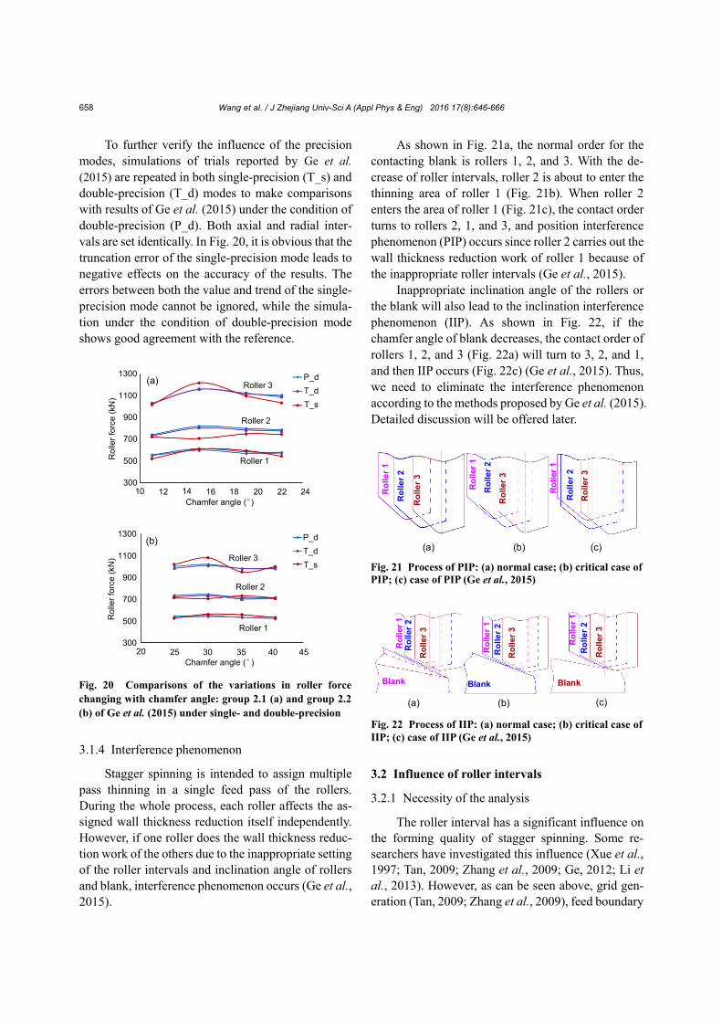
To further verify the influence of the precision modes, simulations of trials reported by Ge et al. (2015) are repeated in both single-precision (T_s) and double-precision (T_d) modes to make comparisons with results of Ge et al. (2015) under the condition of double-precision (P_d). Both axial and radial inter-vals are set identically. In Fig. 20, it is obvious that the truncation error of the single-precision mode leads to negative effects on the accuracy of the results. The errors between both the value and trend of the single- precision mode cannot be ignored, while the simula-tion under the condition of double-precision mode shows good agreement with the reference.

3.1.4 Interference phenomenon

Stagger spinning is intended to assign multiple pass thinning in a single feed pass of the rollers. During the whole process, each roller affects the as-signed wall thickness reduction itself independently. However, if one roller does the wall thickness reduc-tion work of the others due to the inappropriate setting of the roller intervals and inclination angle of rollers and blank, interference phenomenon occurs (Ge et al., 2015).

As shown in Fig. 21a, the normal order for the contacting blank is rollers 1, 2, and 3. With the de-crease of roller intervals, roller 2 is about to enter the thinning area of roller 1 (Fig. 21b). When roller 2 enters the area of roller 1 (Fig. 21c), the contact order turns to rollers 2, 1, and 3, and position interference phenomenon (PIP) occurs since roller 2 carries out the wall thickness reduction work of roller 1 because of the inappropriate roller intervals (Ge et al., 2015).

Inappropriate inclination angle of the rollers or the blank will also lead to the inclination interference phenomenon (IIP). As shown in Fig. 22, if the chamfer angle of blank decreases, the contact order of rollers 1, 2, and 3 (Fig. 22a) will turn to 3, 2, and 1, and then IIP occurs (Fig. 22c) (Ge et al., 2015). Thus, we need to eliminate the interference phenomenon according to the methods proposed by Ge et al. (2015). Detailed discussion will be offered later.

3.2 Influence of roller intervals

3.2.1 Necessity of the analysis

The roller interval has a significant influence on the forming quality of stagger spinning. Some re-searchers have investigated this influence (Xue et al., 1997; Tan, 2009; Zhang et al., 2009; Ge, 2012; Li et al., 2013). However, as can be seen above, grid gen-eration (Tan, 2009; Zhang et al., 2009), feed boundary

Ro

lle

r 1

Ro

ller

2

Ro

ller

3

Blank

Ro

ller

1R

olle

r 2

Ro

ller

3

Blank

Ro

lle

r 1

Ro

lle

r 2

Ro

ller

3

Blank

(a) (b) (c)

Fig. 22 Process of IIP: (a) normal case; (b) critical case of IIP; (c) case of IIP (Ge et al., 2015)

Ro

ller

1

Ro

lle

r 2

Ro

ller

3

Ro

ller

1

Ro

lle

r 2

Ro

ller

3

Ro

ller

1

Ro

lle

r 2

Ro

ller

3

(a) (b) (c)

Fig. 21 Process of PIP: (a) normal case; (b) critical case of PIP; (c) case of PIP (Ge et al., 2015)

Fig. 20 Comparisons of the variations in roller forcechanging with chamfer angle: group 2.1 (a) and group 2.2(b) of Ge et al. (2015) under single- and double-precision

1300

1100

900

700

500

30010 12 14 16 18 20 22 24

Roller 1

Roller 2

Roller 3

Rol

ler

forc

e (k

N)

Chamfer angle (°)

P_d

T_d

T_s

(a)

1300

1100

900

700

500

30020 25 35 40

Roller 1

Roller 2

Roller 3

Rol

ler

forc

e (k

N)

Chamfer angle (°)

P_d

T_d

T_s

(b)

4530


(Tan, 2009; Zhang et al., 2009; Li et al., 2013), pre-cision mode (Ge, 2012; Li et al., 2013), and time truncation (Li et al., 2013) all have significant influ-ence on the accuracy of the simulation result, while interference can lead to obvious oscillation and mu-tation of roller force as well as significant concave and bulge of blank surface (Tan, 2009; Zhang et al., 2009; Ge, 2012; Li et al., 2013). The reliability of simulation is therefore influenced.

Table 6 shows the group of trials to investigate the influence of roller intervals, which are identical to the trails designed by Li et al. (2013).

For validation, we compare three roller forces of simulation results with those of Li et al. (2013) under identical setting of the roll intervals. As shown in Fig. 23, the results appear to be in good agreement, and the errors of the three rollers are 2.50%, 2.70%, and 2.53%, respectively.

As can be seen from Fig. 16, time truncation has been observed in Li et al. (2013). The artificially shortened simulation time has failed to observe the influence of the interference phenomenon. Full sim-ulation of the designed model of Li et al. (2013) has been conducted in this study.

Obvious oscillation and mutation of the roller force appear (Fig. 24), which leads to significant convex and concave shapes of blank surface (Fig. 25).

Table 6 Group 1 axial roller interval distribution of Li et al. (2013) (radial roller intervals ∆t1=2.4 mm, ∆t2=1.7 mm, and ∆t3 =1.3 mm, roller chamfer angle α1=α2=α3=28°)

Trial Axial interval (mm) 1 1.0 2 2.0 3 3.0 4 4.0 5 5.0

50010001500200025003000350040004500

00 50 100 150 200

Roller 1Roller 2Roller 3

50010001500200025003000350040004500

00 50 100 150 200


300600900

12001500180021002400

00 50 100 150 200

Rol

ler

forc

e (K

N)

200400600800

1000120014001600

00 50 100 150 200



Rol

ler

forc

e (

KN

)

200

400

600800

10001200

0


0 50 100 150 200Stroke of rollers (mm)

Rol

ler

forc

e (K

N)

Ro

ller

forc

e (K

N)

Rol

ler

forc

e (K

N)


(a) (b)

(d)(c)

(e)


Stroke of rollers (mm) Stroke of rollers (mm)

Fig. 24 Variations of roller force of eachdesigned trial under full simulation situation (a) Trial 1; (b) Trial 2; (c) Trial 3; (d) Trial 4;(e) Trial 5

Fig. 23 Comparison of the simulation results with those of Li et al. (2013) on the ratio of axial force to radial force (a) Roller 1; (b) Roller 2; (c) Roller 3

Result of roller 1

Simulation result

Ra

tio o

f for

ce

0.40.50.6

0.70.8

0.91.01.11.2

0 2 4 6 8Axial interval (mm)

Result of roller 2

Simulation resultRa

tio o

f for

ce

0.40.50.6

0.70.8

0.91.01.11.2


Result of roller 3

Simulation result


Rat

io o

f fo

rce

0.40.50.6

0.70.8

0.91.01.11.2(a) (b) (c)


It evidently deviates from the original purpose of using three rollers.

According to Ge et al. (2015), when attack angle α1=α2=α3, the formula to avoid PIP is

1 1 1 1 1(1 cos )/sin cot ,i i i i i iC t i=1, 2. (15)

Inserting ρ2=ρ3=5 mm, α2=α3=28°, ∆t2=1.7 mm,

and ∆t3=1.3 mm in Eq. (15), the minimum axial in-tervals without PIP in group 1 are C1=4.4439 mm and

C2=3.6916 mm. It is obvious that interference occurs in the designed trials. Fig. 26 shows the actual roller position of each trial. Except trial 5, all the trials in the two groups have different interference phenomena.

In Figs. 26a–26c, roller 3 enters the thinning part of roller 2, while roller 2 enters that of roller 1, and the interference order is rollers 3, 2, 1. Similarly, the interference order is rollers 2, 1, 3 in Fig. 26d. The accuracy of the result of the roller force and wall thickness reported by Li et al. (2013) was influenced by the displacement boundary, single-precision mode, and time truncation. Meanwhile, interference phe-nomenon occurred in most of the designed two group trials. The reliability of the trends of time-history parameter will be affected significantly due to the coupling of the interference phenomenon.

Others have also found different interference phenomena (Tan, 2009; Zhang et al., 2009; Ge, 2012), where the calculation process was similar as before. For example, in the analyses of the roller interval of Ge (2012), obvious oscillation and mutation could also be observed.

It shows that the roller intervals have a significant influence on results of modeling and will affect the accuracy and reliability of the results. It is necessary to carry out work to improve the current results.

3.2.2 Influence of roller intervals without interference

In view of the accuracy and reliability of the results in previous studies, which are influenced by

Fig. 25 Wall thickness variations under full simulationsituation: (a) wall thickness; (b) cross sections of each trial

0 50 100 150 200Axial distance (mm)

Wal

l th

ickn

ess

(mm

)

2

3

4

5

6

7

8

9 Trial 1Trial 2Trial 3

Trial 4Trial 5

Trial 1

Trial 2

Trial 3

Trial 4

Trial 5

(a)

(b)

Fig. 26 Actual roller position of group 1 (a) PIP: rollers 3, 2, 1; (b) PIP: rollers 3, 2, 1; (c) PIP: rollers 3, 2, 1; (d) PIP: rollers 2, 1, 3; (e) No interference phenomenon

Trial 1

Blank

C1 C2C1 C2

Blank

Trial 2C1 C2

Blank

Trial 3

C1C2

Blank

Trial 4C1 C2

Blank

Trial 5

(a) (b) (c)

(d) (e)


above problems, trials are designed to analyze the influence of roller intervals under full model, feed boundary, double-precision, full simulation, and no interference conditions. Tables 7 and 8 show the in-tervals of simulation, where A denotes the axial interval, and R=(Δt1, Δt2, Δt3) denotes the radial roller intervals of rollers 1, 2, and 3.

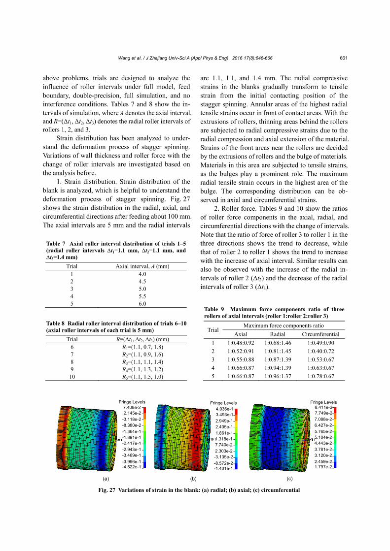
Strain distribution has been analyzed to under-stand the deformation process of stagger spinning. Variations of wall thickness and roller force with the change of roller intervals are investigated based on the analysis before.

1. Strain distribution. Strain distribution of the blank is analyzed, which is helpful to understand the deformation process of stagger spinning. Fig. 27 shows the strain distribution in the radial, axial, and circumferential directions after feeding about 100 mm. The axial intervals are 5 mm and the radial intervals

are 1.1, 1.1, and 1.4 mm. The radial compressive strains in the blanks gradually transform to tensile strain from the initial contacting position of the stagger spinning. Annular areas of the highest radial tensile strains occur in front of contact areas. With the extrusions of rollers, thinning areas behind the rollers are subjected to radial compressive strains due to the radial compression and axial extension of the material. Strains of the front areas near the rollers are decided by the extrusions of rollers and the bulge of materials. Materials in this area are subjected to tensile strains, as the bulges play a prominent role. The maximum radial tensile strain occurs in the highest area of the bulge. The corresponding distribution can be ob-served in axial and circumferential strains.

2. Roller force. Tables 9 and 10 show the ratios of roller force components in the axial, radial, and circumferential directions with the change of intervals. Note that the ratio of force of roller 3 to roller 1 in the three directions shows the trend to decrease, while that of roller 2 to roller 1 shows the trend to increase with the increase of axial interval. Similar results can also be observed with the increase of the radial in-tervals of roller 2 (∆t2) and the decrease of the radial intervals of roller 3 (∆t3).

Table 9 Maximum force components ratio of three rollers of axial intervals (roller 1:roller 2:roller 3)

TrialMaximum force components ratio

Axial Radial Circumferential

1 1:0.48:0.92 1:0.68:1.46 1:0.49:0.90

2 1:0.52:0.91 1:0.81:1.45 1:0.40:0.72

3 1:0.55:0.88 1:0.87:1.39 1:0.53:0.67

4 1:0.66:0.87 1:0.94:1.39 1:0.63:0.67

5 1:0.66:0.87 1:0.96:1.37 1:0.78:0.67

Table 8 Radial roller interval distribution of trials 6–10 (axial roller intervals of each trial is 5 mm)

Trial R=(Δt1, Δt2, Δt3) (mm) 6 R1=(1.1, 0.7, 1.8) 7 R2=(1.1, 0.9, 1.6) 8 R3=(1.1, 1.1, 1.4) 9 R4=(1.1, 1.3, 1.2)

10 R5=(1.1, 1.5, 1.0)

Table 7 Axial roller interval distribution of trials 1–5 (radial roller intervals ∆t1=1.1 mm, ∆t2=1.1 mm, and ∆t3=1.4 mm)

Trial Axial interval, A (mm) 1 4.0 2 4.5 3 5.0 4 5.5 5 6.0

Fig. 27 Variations of strain in the blank: (a) radial; (b) axial; (c) circumferential

Fringe Levels

2.145e-2

-3.118e-2-8.380e-2

-1.364e-1-1.891e-1-2.417e-1

-2.943e-1-3.469e-1

-3.996e-1-4.522e-1

7.408e-2Fringe Levels

3.493e-1

2.949e-12.405e-1

1.861e-11.318e-17.740e-2

2.303e-2-3.135e-2

-8.572e-2-1.401e-1

4.036e-17.749e-2

7.088e-26.427e-2

5.765e-25.104e-24.443e-2

3.781e-23.120e-2

2.459e-21.797e-2

8.411e-2Fringe Levels

(a) (b) (c)


Figs. 28a–28c show the variations of roller force components of trials 1–5 in the axial, radial, and cir-cumferential directions in this study with the change of axial intervals, respectively, corresponding to the result of Li et al. (2013). Three force components of rollers 1 and 3 show the trend to decrease with the increase of axial intervals, while roller 2 shows the trend to increase. Radial roller force is the highest and circumferential force is the lowest. The circumferen-tial force is much smaller than the axial and radial forces. Forces of roller 3 with the largest amplitude change fastest. Forces of rollers 1 and 3 are more sensitive to the change of the axial intervals. It can also be observed that the difference between the forces of rollers 1 and 2 becomes smaller with the increase of axial intervals, while that of rollers 1 and 3 shows the trend to become larger.

Fig. 29 shows the variations of roller forces components of trials 6–10 with the change of radial intervals. With the increase of ∆t2 and decrease of ∆t3, three components of rollers 2 and 3, respectively, show the trend to increase and decrease gradually. The axial and circumferential forces of roller 1 decrease first and then increase, while the radial force decreases gradu-ally. The difference between rollers 1 and 2 shows the trend to decrease first and then increase with the change of radial intervals, and so is that between rollers 1 and 3. For stagger spinning, equilibrium of the three roller forces has a significant influence on the quality of the spun products. The variation trend of the roller forces above indicates that there is an optimal variation of roller intervals to get similar roller forces based on the distribution trend between the intervals and forces in the axial and radial directions.

3. Wall thickness. As shown in Fig. 30, com-pared with the wall thickness curve under interference condition in Fig. 25, both groups of simulation maintain a good smooth state, and the fluctuation is small in the whole region. Trial 1 has the maximum reduction rate of 31.75%, and trial 5 has the smallest reduction rate of 31.29%. Each simulation result of wall thickness reduction shows good correlation with the designed reduction rate. At the same time, as shown in Fig. 30, obvious wall thickness differences occur in the beginning and ending areas.

Table 10 Maximum force components ratio of three rollers of radial intervals (roller 1:roller 2:roller 3)

Trial Maximum force components ratio

Axial Radial Circumferential

6 1:0.43:1.33 1:0.63:1.52 1:0.27:1.03

7 1:0.5:1.11 1:0.74:1.42 1:0.41:0.82

8 1:0.55:0.88 1:0.87:1.39 1:0.53:0.67

9 1:0.63:0.66 1:0.98:1.36 1:0.66:0.57

10 1:0.60:0.45 1:1.15:1.42 1:0.66:0.45

Fig. 28 Tool force comparison with changing of axial intervals: (a) axial; (b) radial; (c) circumferential

3 74 5 610

20

30

40

50

Fo

rce

(KN

)

Axial interval (mm)

Roller 1

Roller 2

Roller 3

3 74 5 6

Axial interval (mm)

Roller 1

Roller 2

Roller 3

40

80

120

160

200

Fo

rce

(KN

)

Roller 1

Roller 2

Roller 3

0.4

0.8

1.2

1.6

2.0

For

ce (

KN

)

3 74 5 6Axial interval (mm)

(a) (b) (c)

Fig. 29 Tool force comparison with changing of radial intervals: (a) axial; (b) radial; (c) circumferential

0.5 1.30.7 0.9 1.1Radical interval between rollers 1 and 2 (mm)

1.5 1.7

Radical interval between rollers 2 and 3 (mm)

0

15

30

45

60

752 1.21.8 1.6 1.4 1.0 0.8

Fo

rce

(K

N)

2 1.21.8 1.6 1.4 1.0 0.8

0.5 1.30.7 0.9 1.1 1.5 1.720

60

100

140

180

220

For

ce (

KN

)

0.5 1.30.7 0.9 1.1 1.5 1.7

2 1.21.8 1.6 1.4 1.0 0.8

0.2

0.6

1.0

1.4

1.8

2.2

For

ce (

KN

)

(a) (b) (c)Roller 1

Roller 2

Roller 3

Roller 1

Roller 2

Roller 3

Roller 1

Roller 2

Roller 3

Radical interval between rollers 2 and 3 (mm) Radical interval between rollers 2 and 3 (mm)

Radical interval between rollers 1 and 2 (mm) Radical interval between rollers 1 and 2 (mm)


Figs. 31 and 32 show the variations of wall thickness along the axial direction with changing of axial and radial intervals in the beginning and ending areas, respectively, corresponding to that of Li et al. (2013). The wall thicknesses of trials 2, 3, and 4 de-crease slowly to the minimum and then increase gradually after remaining steady at about 10 mm (Fig. 31a). The three trials change smoothly during the beginning areas. Obvious fluctuations appear within the range of 5–15 mm for trials 1 and 5. With the increase of axial intervals, the wall thickness fluctuation generally shows a trend to decrease first and then to increase in the beginning areas of the blank.

Fig. 31b shows the variations of wall thickness with the change of radial intervals. The thinning ratios of wall thickness in this area are 34.05%, 33.88%, 33.76%, 33.45%, and 33.32%.

The trends of wall thickness variations are sim-ilar; the thinning ratio of the wall thickness decreases gradually with the increase of ∆t2 and decrease of ∆t3. With the increase of axial intervals, the minimum wall thickness of each trial increases gradually. A similar phenomenon can be observed with the decrease of ∆t2 and increase of ∆t3, as shown in Fig. 32.

Fig. 30 Variations of wall thickness with changing of rollerintervals: (a) axial; (b) radial

6

7

8

9

10

11

0 20 40 60 80 100 120 140

Axial distance (mm)

Wal

l th

ickn

ess

(mm

)

Trial 6 (R1)

Trial 7 (R2)

Trial 8 (R3)

Trial 9 (R4)Trial 10 (R5)

B

A

(a)

(b)

6

7

8

9

10

11

0 20 40 60 80 100 120 140

Axial distance (mm)

Wal

l thi

ckne

ss (

mm

)

Trial 1 (A=4.0 mm)

Trial 2 (A=4.5 mm)

Trial 3 (A=5.0 mm)

Trial 4 (A=5.5 mm)

Trial 5 (A=6.0 mm)

A

B

Fig. 31 Variations of wall thickness with changing of roller intervals in the beginning areas of blank: (a) axial; (b) radial

(a)

(b)

7.6

7.7

7.8

7.9

8.0

8.1

8.2

0 5 10 15 20 25 30 35

Axial distance (mm)

Wa

ll th

icjn

ess

(m

m)

Trial 6 (R1)

Trial 7 (R2)

Trial 8 (R3)

Trial 10 (R5)

Trial 9 (R4)

7.6

7.7

7.8

7.9

8.0

8.1

8.2

8.3

0 5 10 15 20 25 30 35

Axial distance (mm)

Wal

l thi

ckne

ss (

mm

)

Trial 1 (A=4.0 mm)

Trial 2 (A=4.5 mm)

Trial 3 (A=5.0 mm)

Trial 4 (A=5.5 mm)

Trial 5 (A=6.0 mm)

Fig. 32 Variations of wall thickness with changing of roller intervals in the ending areas of blank: (a) axial; (b) radial

7.8

8.0

8.2

8.4

8.6

8.8

9.0

9.2

110 115 120 125 130 135 140Axial distance (mm)

Wal

l thi

ckne

ss (

mm

)

Trial 6 (R1)

Trial 7 (R2)

Trial 8 (R3)

Trial 10 (R5)

Trial 9 (R4)

(b)

(a)

7.8

8.0

8.2

8.4

8.6

8.8

9.0

9.2

110 115 120 125 130 135 140Axial distance (mm)

Wal

l th

ickn

ess

(mm

)

Trial 1 (A=4.0 mm)

Trial 2 (A=4.5 mm)

Trial 3 (A=5.0 mm)

Trial 4 (A=5.5 mm)

Trial 5 (A=6.0 mm)


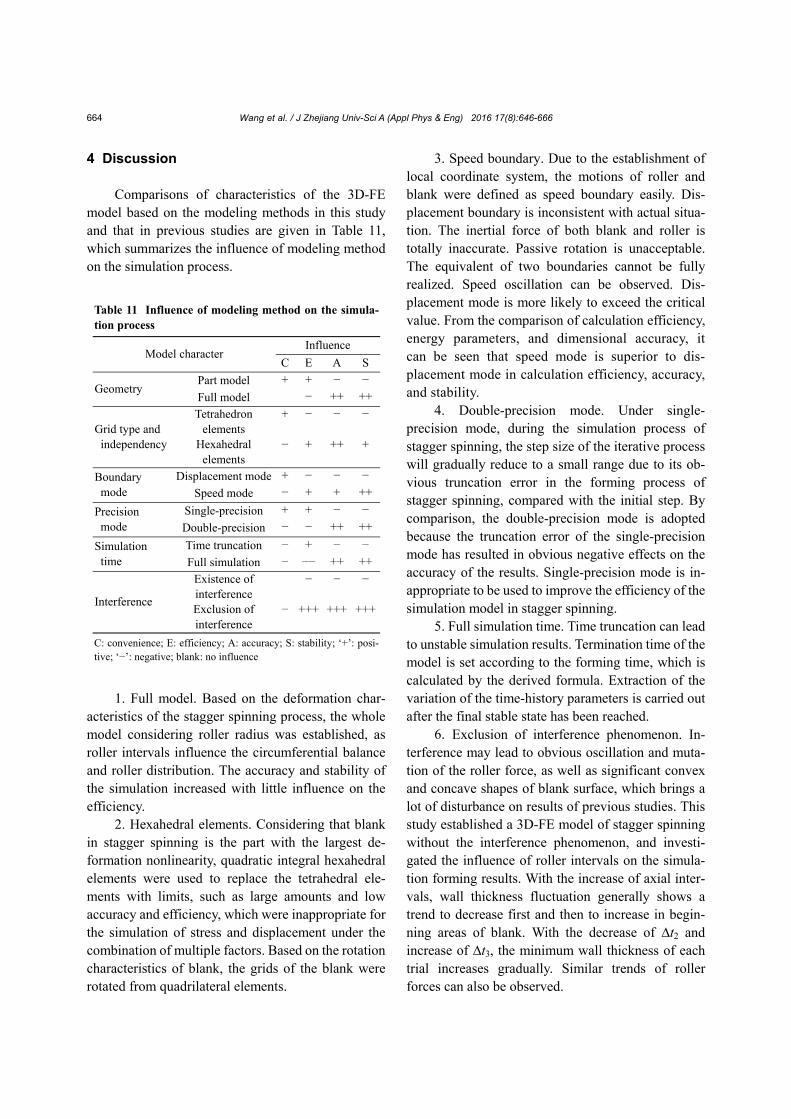
4 Discussion Comparisons of characteristics of the 3D-FE

model based on the modeling methods in this study and that in previous studies are given in Table 11, which summarizes the influence of modeling method on the simulation process.

1. Full model. Based on the deformation char-

acteristics of the stagger spinning process, the whole model considering roller radius was established, as roller intervals influence the circumferential balance and roller distribution. The accuracy and stability of the simulation increased with little influence on the efficiency.

2. Hexahedral elements. Considering that blank in stagger spinning is the part with the largest de-formation nonlinearity, quadratic integral hexahedral elements were used to replace the tetrahedral ele-ments with limits, such as large amounts and low accuracy and efficiency, which were inappropriate for the simulation of stress and displacement under the combination of multiple factors. Based on the rotation characteristics of blank, the grids of the blank were rotated from quadrilateral elements.

3. Speed boundary. Due to the establishment of local coordinate system, the motions of roller and blank were defined as speed boundary easily. Dis-placement boundary is inconsistent with actual situa-tion. The inertial force of both blank and roller is totally inaccurate. Passive rotation is unacceptable. The equivalent of two boundaries cannot be fully realized. Speed oscillation can be observed. Dis-placement mode is more likely to exceed the critical value. From the comparison of calculation efficiency, energy parameters, and dimensional accuracy, it can be seen that speed mode is superior to dis-placement mode in calculation efficiency, accuracy, and stability.

4. Double-precision mode. Under single- precision mode, during the simulation process of stagger spinning, the step size of the iterative process will gradually reduce to a small range due to its ob-vious truncation error in the forming process of stagger spinning, compared with the initial step. By comparison, the double-precision mode is adopted because the truncation error of the single-precision mode has resulted in obvious negative effects on the accuracy of the results. Single-precision mode is in-appropriate to be used to improve the efficiency of the simulation model in stagger spinning.

5. Full simulation time. Time truncation can lead to unstable simulation results. Termination time of the model is set according to the forming time, which is calculated by the derived formula. Extraction of the variation of the time-history parameters is carried out after the final stable state has been reached.

6. Exclusion of interference phenomenon. In-terference may lead to obvious oscillation and muta-tion of the roller force, as well as significant convex and concave shapes of blank surface, which brings a lot of disturbance on results of previous studies. This study established a 3D-FE model of stagger spinning without the interference phenomenon, and investi-gated the influence of roller intervals on the simula-tion forming results. With the increase of axial inter-vals, wall thickness fluctuation generally shows a trend to decrease first and then to increase in begin-ning areas of blank. With the decrease of ∆t2 and increase of ∆t3, the minimum wall thickness of each trial increases gradually. Similar trends of roller forces can also be observed.

Table 11 Influence of modeling method on the simula-tion process

Model character Influence

C E A S

Geometry Part model + + − −

Full model − ++ ++

Grid type and independency

Tetrahedron elements

+ − − −

Hexahedral elements

− + ++ +

Boundary mode

Displacement mode + − − −

Speed mode − + + ++

Precision mode

Single-precision + + − −

Double-precision − − ++ ++

Simulation time

Time truncation − + − −

Full simulation − −− ++ ++

Interference

Existence of interference

− − −

Exclusion of interference

− +++ +++ +++

C: convenience; E: efficiency; A: accuracy; S: stability; ‘+’: posi-tive; ‘−’: negative; blank: no influence


5 Conclusions A modified 3D-FE model with better accuracy

and stability of stagger spinning was established in LS-DYNA. Influence of inappropriate simplified methods, which occurred in previous studies, were analyzed and summarized. Characteristics of the model include full model, hexahedral element, speed boundary mode, full simulation, double-precision mode, and exclusion of interference phenomenon. The grid independence, the energy criteria, the pro-cessing parameters, the thickness results of plastic strain, the swelling size, and the uplift coefficient were compared with simulation and experiments to verify the improved model. Then, the modified model with better accuracy and stability was applied to in-vestigate the influence of intervals. Strain distribution, wall thickness, and roller force variations were ob-tained to improve the reported results.

Previous studies on modeling methods have made great contributions for the FE simulation model. Though the modeling methods for stagger spinning offered here have made some improvements, there is still much work to be done, such as more experi-mental assistance, consideration of clamping force, and multi-physics coupling, to make further im-provement of the modeling methods for stagger spinning.

References Cheng, X.Q., Sun, L.Y., Xia, Q.X., 2011. Processing parame-

ters optimization for stagger spinning of trapezoidal inner gear. Advanced Materials Research, 189-193:2754-2758. http://dx.doi.org/10.4028/www.scientific.net/AMR.189-193.2754

Essa, K., Hartley, P., 2010. Optimization of conventional spinning process parameters by means of numerical sim-ulation and statistical analysis. Proceedings of the Insti-tution of Mechanical Engineers, Part B: Journal of En-gineering Manufacture, 224(11):1691-1705. http://dx.doi.org/10.1243/09544054JEM1786

Fazeli, A.R., Ghoreishi, M., 2009. Investigation of effective parameters on surface roughness in thermomechanical tube spinning process. International Journal of Material Forming, 2(4):261-270. http://dx.doi.org/10.1007/s12289-009-0420-1

Fazeli, A.R., Ghoreishi, M., 2011. Statistical analysis of di-mensional changes in thermomechanical tube-spinning process. The International Journal of Advanced Manu-facturing Technology, 52(5):597-607. http://dx.doi.org/10.1007/s00170-010-2780-6

Gadala, M.S., Wang, J., 1999. Simulation of metal forming processes with finite element methods. International Journal for Numerical Methods in Engineering, 44(10): 1397-1428. http://dx.doi.org/10.1002/(SICI)1097-0207(19990410)44:10<1397::AID-NME496>3.0.CO;2-3

Ge, D., 2012. Research on FEM Numerical Simulation of Power Spinning of Rod Bushing and Process Parameters. MS Thesis, North University of China, Taiyuan, China (in Chinese).

Ge, T., Wang, J., Lu, G.D., et al., 2015. A study of influence of interference phenomenon on stagger spinning of thin- walled tube. Proceedings of the Institution of Mechanical Engineers, Part B: Journal of Engineering Manufacture, 229(12):2265-2283. http://dx.doi.org/10.1177/0954405414543487

Hua, F.A., Yang, Y.S., Zhang, Y.N., et al., 2005. Three- dimensional finite element analysis of tube spinning. Jorunal of Materials Processing Technology, 168(1): 68-74. http://dx.doi.org/10.1016/j.jmatprotec.2004.10.014

Huang, L., Yang, H., Zhan, M., 2008. 3D-FE modeling method of splitting spinning. Computational Materials Science, 42(4):643-652. http://dx.doi.org/10.1016/j.commatsci.2007.09.012

Lexian, H., Dariani, B.M., 2008. An analytical contact model for finite element analysis of tube spinning process. Proceedings of the Institution of Mechanical Engineers, Part B: Journal of Engineering Manufacture, 222(11): 1375-1385. http://dx.doi.org/10.1243/09544054JEM1202

Lexian, H., Dariani, B.M., 2009. Effect of roller nose radius and release angle on the forming quality of a hot-spinning process using a non-linear finite element shell analysis. Proceedings of the Institution of Mechanical Engineers, Part B: Journal of Engineering Manufacture, 223(6):713- 722. http://dx.doi.org/10.1243/09544054JEM1445

Li, K.Z., Hao, N.H., Lu, Y., et al., 1998. Research on the dis-tribution of the displacement in backward tube spinning. Journal of Materials Processing Technology, 79(1-3): 185-188. http://dx.doi.org/10.1016/S0924-0136(98)00009-0

Li, Y., Wang, J., Lu, G.D., et al., 2013. Three-dimensional finite element analysis of effects of roller intervals on tool forces and wall thickness in stagger spinning of thin- walled tube. Proceedings of the Institution of Mechanical Engineers, Part C: Journal of Mechanical Engineering Science, 227(7):1429-1440. http://dx.doi.org/10.1177/0954406212466518

Li, Y., Wang, J., Lu, G.D., et al., 2014. A numerical study of the effects of roller paths on dimensional precision in die-less spinning of sheet metal. Journal of Zhejiang University- SCIENCE A (Applied Physics & Engineering), 15(6):432- 446. http://dx.doi.org/10.1631/jzus.A1300405


Liu, F., 2006. Finite Element Analysis of Process Power- Spinning for Cylindrical Part. MS Thesis, Sichuan Uni-versity, Chengdu, China (in Chinese).

LSTC (Livermore Software Technology Corporation), 2007. LS-DYNA Keyword User’s Manual (Version 971). LSTC, Livermore, USA.

Ma, S., 2008. Research on the Forming Law of Aluminum Alloy Draw-spinning. MS Thesis, Yanshan University, Qinhuangdao, China (in Chinese).

Mohebbi, M.S., Akbarzadeh, A., 2010. Experimental study and FEM analysis of redundant strains in flow forming of tubes. Journal of Materials Processing Technology, 210(2):389-395. http://dx.doi.org/10.1016/j.jmatprotec.2009.09.028

Tan, W., 2009. Research on 1Cr18Ni9 Stainless Steel Tube Stagger Spinning. MS Thesis, Shenyang Ligong Univer-sity, Shenyang, China (in Chinese).

Wong, C.C., Dean, T.A., Lin, J., 2003. A review of spinning, shear forming and flow forming processes. International Journal of Machine Tools and Manufacture, 43(14): 1419-1435. http://dx.doi.org/10.1016/S0890-6955(03)00172-X

Xia, Q.X., Zhang, P., Cheng, X.Q., et al., 2012. Orthogonal experimental study on forming process parameters of tube stagger spinning. Forging & Stamping Technology, 37(06):42-46.

Xu, W.C., Shan, D.B., Lu, Y., et al., 2005. Research on the characteristics of hot deformation in BT20 titanium alloy and its optimum spinning temperature range. Journal of Materials Science & Technology, 21(6):807-812. http://dx.doi.org/10.3321/j.issn:1005-0302.2005.06.007

Xue, K.M., Lu, Y., Zhao, X.M., 1997. The disposal of key problems in the FEM analysis of tube stagger spinning. Journal of Materials Processing Technology, 69(1-3): 176-179. http://dx.doi.org/10.1016/S0924-0136(97)00014-9

Yang, H., Huang, L., Zhan, M., 2010. Coupled thermos- mechanical FE simulation of the hot splitting spinning process of magnesium alloy AZ31. Computational Ma-terials Science, 47(3):857-866. http://dx.doi.org/10.1016/j.commatsci.2009.11.014

Zhang, J., Zhan, M., Yang, H., et al., 2012. 3D-FE modeling for power spinning of large ellipsoidal heads with varia-ble thicknesses. Computational Materials Science, 53(1): 303-313. http://dx.doi.org/10.1016/j.commatsci.2011.08.010

Zhang, N., Tan, W., Li, Y.H., et al., 2009. Numerical simula-tion and spinning force analysis for tube stagger spinning. Transactions of Shenyang Ligong University, 28(05):

55-58. Zhao, Y., Li, Y., 2008. Forming Technology and Application.

Machinery Industry Press, Beijing, China (in Chinese). Zoghi, H., Arezoodar, A.F., 2013. Finite element study of

stress and strain state during hot tube necking process. Proceedings of the Institution of Mechanical Engineers, Part B: Journal of Engineering Manufacture, 227(4): 551-564. http://dx.doi.org/10.1177/0954405413476495

Zoghi, H., Arezoodar, A.F., Sayeaftabi, M., 2013. Enhanced finite element analysis of material deformation and strain distribution in spinning of 42CrMo steel tubes at elevated temperature. Materials & Design, 47:234-242. http://dx.doi.org/10.1016/j.matdes.2012.11.049

中文概要

题目：薄壁筒形件错距旋压有限元仿真模型构建方法

研究

目的：探究错距旋压仿真模型关键特性参数影响，改进

建模方法，克服现有模型方案的缺陷，构建更准

确、可靠和稳定的错距旋压有限元仿真模型。

创新点：1. 提供包括全模型、六面体离散、速度边界、全

仿真、双精度和无干涉模型等在内的改进有限元

模型构建方法；2. 基于所构建的改进模型，完善

错距值对成型过程影响的现有结论。

方法：1. 通过能量、网格独立性和过程参数分析，验证

改进有限元模型的可行性和可靠性； 2. 通过对比

仿真和数据分析，获得边界模式、精度模式、时

间截断和错距干涉对仿真结果的影响；3. 通过仿

真模拟，完善现有受干涉、单精度、时间截断和

位移边界影响的错距值研究成果。

结论：1. 速度边界模式较之位移边界模式具有更高的计

算精度和效率；2. 时间截断不能确保获取稳态结

果，不利于计算的准确性和稳定性；3. 截断误差

对错距旋压成型结果影响显著，计算过程中应采

用双精度模式；4. 错距干涉严重干扰计算的正确

性和可靠性，应在实验设计阶段予以排除；5. 针

对现有错距值研究受干涉、单精度、时间截断和

位移边界影响的现状，基于改进模型，完善错距

影响结论（表 11）。

关键词：错距旋压；有限元三维建模；错距值；薄壁筒

形件

a study of 3d finite element modeling method for stagger ... · a study of 3d finite element...

Documents