A Study of Dynamic Meta-Learning for

Failure Prediction in Large-Scale Systems

Zhiling Lan, Jiexing Gu, Ziming Zheng

Illinois Institute of Technology, Chicago, IL 60616

Rajeev Thakur, Susan Coghlan

Argonne National Laboratory, Argonne, IL, 60439

Abstract

Despite years of study on failure prediction, it remains an open problem, especiallyin large-scale systems composed of vast amount of components. In this paper, wepresent a dynamic meta-learning framework for failure prediction. It intends to notonly provide reasonable prediction accuracy, but also be of practical use in realisticenvironments. Two key techniques are developed to address technical challenges offailure prediction. One is meta-learning to boost prediction accuracy by combiningthe benefits of multiple predictive techniques. The other is a dynamic approach todynamically obtain failure patterns from a changing training set and to dynamicallyextract effective rules by actively monitoring prediction accuracy at runtime. Wedemonstrate the effectiveness and practical use of this framework by means of realsystem logs collected from the production Blue Gene/L systems at Argonne NationalLaboratory and San Diego Supercomputer Center. Our case studies indicate thatthe proposed mechanism can provide reasonable prediction accuracy by forecastingup to 82% of the failures, with a runtime overhead less than 1.0 minute.

Key words: failure prediction, meta-learning, dynamic techniques, large-scalesystems, Blue Gene

Email addresses: {lan,jgu5,zzheng11}@iit.edu (Zhiling Lan, Jiexing Gu,Ziming Zheng), {thakur,smc}@mcs.anl.gov (Rajeev Thakur, Susan Coghlan).

Preprint submitted to Elsevier 16 March 2010

1 Introduction

1.1 Motivations

To meet the insatiable demand in science and engineering, supercomputerscontinue to grow in size. Production systems with tens to hundreds of thou-sands of computing nodes are being designed and deployed [30]. Such a scale,combined with the ever-growing system complexity, is introducing a key chal-lenge — reliability — in the field of high performance computing (HPC).Despite great efforts on the design of ultra-reliable components, the increaseof system size and complexity has outpaced the improvement of component re-liability. Recent studies have pointed out that the mean-time-between-failure(MTBF) of teraflop and soon-to-be-deployed petaflop machines are only onthe order of 10 - 100 hours [4,41,22].

To address the reliability problem, considerable research has been done toimprove fault resilience of computer systems and their applications throughvarious technologies. Representative works include failure-aware resource man-agement and scheduling [10,15,20], checkpointing [6,18,24,38], proactive oradaptive runtime resilience support [14,29]. The advance of these technolo-gies, however, greatly depends on whether we can predict the occurrence offailure, i.e., failure prediction. For example, proactive fault tolerant methods,such as preemptive process migration, require failure forecasting to enablecost-effective failure avoidance. For reactive methods such as checkpointing,an efficient failure prediction could substantially reduce their operational costby telling when and where to perform checkpoints, rather than blindly invok-ing actions periodically with an unwisely chosen frequency.

Despite years of study on failure prediction, it remains an unsolved problem,especially in large-scale systems composed of substantial amount of compo-nents. We summarize its key challenges from two aspects. First is predic-tion accuracy. Existing studies mainly concentrate on exploring one specificmethod to capture and discover failure patterns. As a matter of fact, in alarge-scale system the sources of failures are numerous and complex, thus itis improper to expect a single method to capture all of failures alone. Forexample, many rule-based classifiers emphasize on discovering correlation re-lationships between warning messages and fatal events for failure prediction[39,23]. As we will show in our experiments, they are limited by the amount offatal events occurring without any precursor warnings. Hence, relying on thesemethods alone is insufficient to provide an effective failure forecasting. Further,hardware and software upgrades are common at supercomputing centers, andsystem workloads tend to vary during system operation. These changes candrastically alter system behaviors [41]. As a result, static analysis that uses

2

a fixed set of historic data to learn failure patterns cannot adapt to systemchanges at runtime, thereby being incapable of providing accurate forecasting.

The next is with respect to practical use. While many predictive models havebeen presented so far, most of them merely focus on the algorithm-level im-provement and are too complicated to be of practical use for online failureprediction [17,40]. In addition, to obtain sufficient failure patterns, many pre-dictive methods require a long training phase (e.g., one or more years), therebybeing unable to provide prediction service for a long period of time [8]. Giventhat most systems at supercomputing centers only have a couple of years inproduction, this requirement must be removed.

1.2 Main Contributions

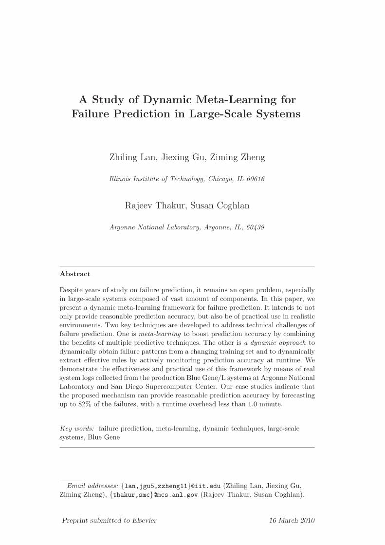
In this study, we present a dynamic meta-learning framework for online failureprediction in large-scale systems. It intends to provide reasonable predictionaccuracy, as well as be of practical use in realistic environments. Our frame-work consists of two parts to process and analyze system events: one is topreprocess system events by means of event categorization and filtering (i.e.,data preprocessing), and the other is to examine the cleaned events for gen-erating failure patterns and triggering failure warnings through continuousruntime event analysis (i.e., failure prediction). These two parts, along withtheir main components, are illustrated in Figure 1. The details of the maincomponents will be described in Section 3 - 4.

Our method employs two key techniques to address the challenges listed above.First, meta-learning is explored to boost prediction accuracy by combining thebenefits of multiple predictive methods. It enables us to discover a variety offailure patterns in large-scale systems, without constructing complex models ofthe underlying system. In this study, we integrate three widely-used predictivemethods, namely association rule based learner [23,28], statistical rule basedlearner [16], and probability distribution [4], in the framework by applying asimple yet efficient ensemble learning method. Next, a dynamic mechanism isadopted to trigger relearning periodically and to adaptively extract effectiverules of failure patterns by actively tracing prediction accuracy.

To demonstrate the effectiveness and practical use of our framework, we eval-uate it with the real RAS (Reliability, Availability and Serviceability) logscollected from the production Blue Gene/L systems at Argonne NationalLaboratory (ANL) and San Diego Supercomputer Center (SDSC). The useof multiple RAS logs is to ensure our framework is not bias to any specific logand thus produces representative results expected in other systems as well.To comprehensively assess our framework, our experiments are structured to

3

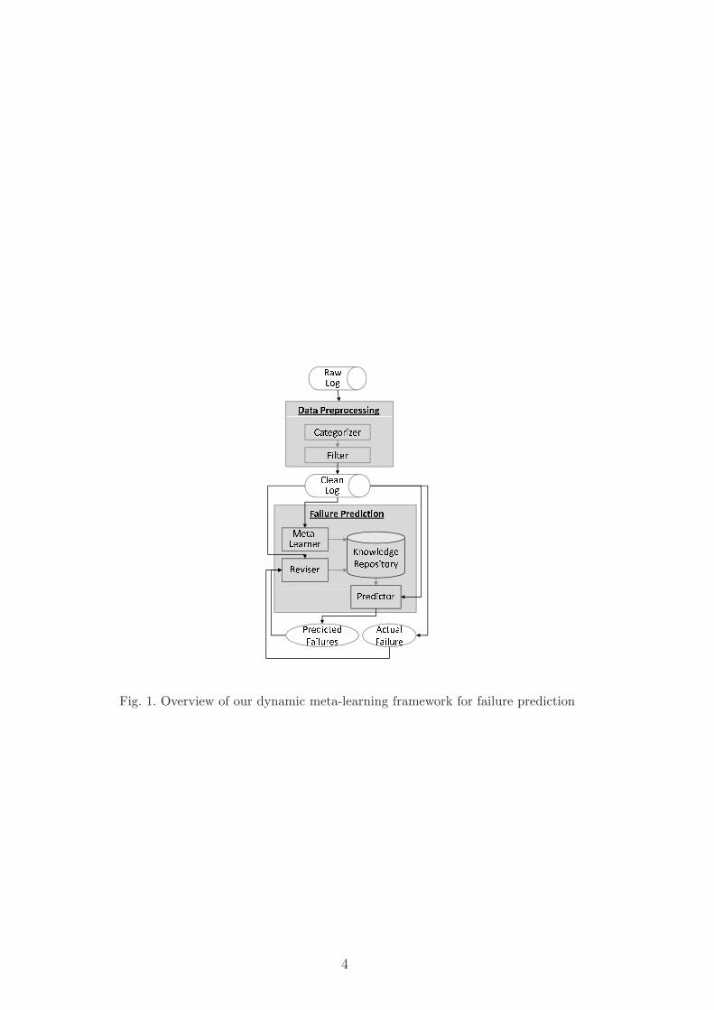
Fig. 1. Overview of our dynamic meta-learning framework for failure prediction

4

answer the following questions:

Q1: How much improvement is achieved by the meta-learning?Q2: How much improvement is achieved by the dynamic approach?Q3: How sensitive is prediction accuracy to prediction window size?Q4: How much runtime overhead is introduced?

Our experiments demonstrate that meta-learning can effectively improve pre-diction accuracy by up to three times, and the dynamic approach is capableof adapting to system changes, even after a major system reconfiguration.For both systems, our method can provide reasonable prediction accuracyby predicting up to 82% of failures, with a runtime overhead less than 1.0minute. Furthermore, prediction accuracy depends on how far away we areinterested in forecasting failures. In general, the larger the window is, thehigher the prediction coverage is, along with a higher false alarm rate. Therules of failure patterns change dramatically during system operation, whichfurther proves that the dynamic approach is indispensable for better predic-tion. Finally, runtime overhead increases with the growing size of the trainingset. Overall speaking, we find that for both systems, the use of recent six-month training set can well balance between prediction accuracy and runtimeoverhead.

We note that three predictive methods, namely association rule based learn-ing, statistical learning, and probability distribution, have been tested in ourexperiments. Rather than focusing on which predictive method is better, thisstudy focuses on providing a general framework to dynamically combine mul-tiple predictive methods for better failure prediction. We believe that otherpredictive methods like [17,37] can be easily integrated into our framework.

1.3 Paper Organization

The rest of the paper is organized as follows. Section 2 gives the backgroundinformation of Blue Gene systems and system logs. Section 3 describes thedetails of data preprocessing, followed by a detailed description of our dynamicmeta-learning method in Section 4. The case studies with real failure logs arepresented in Section 5. Section 6 discusses the related work and points outthe key differences between this work and existing studies. Finally, Section 7summarizes the paper.

5

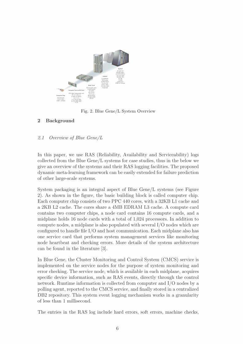
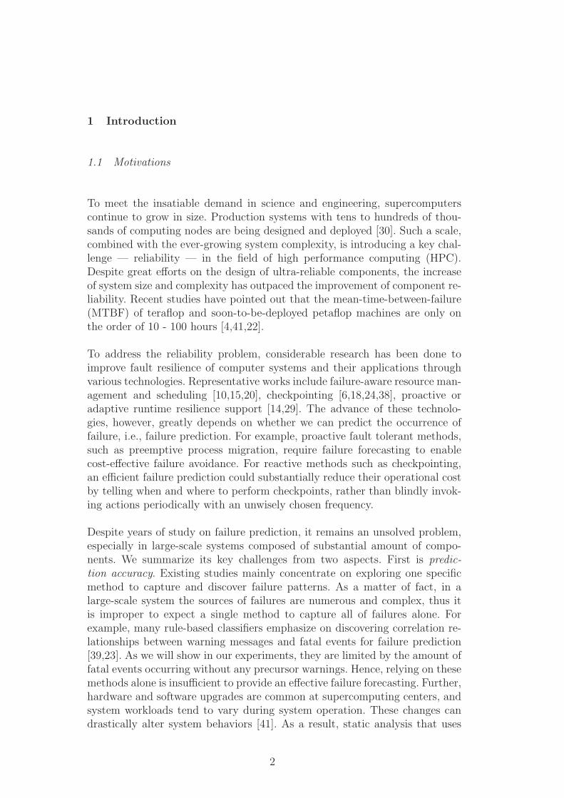
Fig. 2. Blue Gene/L System Overview

2 Background

2.1 Overview of Blue Gene/L

In this paper, we use RAS (Reliability, Availability and Serviceability) logscollected from the Blue Gene/L systems for case studies, thus in the below wegive an overview of the systems and their RAS logging facilities. The proposeddynamic meta-learning framework can be easily extended for failure predictionof other large-scale systems.

System packaging is an integral aspect of Blue Gene/L systems (see Figure2). As shown in the figure, the basic building block is called computer chip.Each computer chip consists of two PPC 440 cores, with a 32KB L1 cache anda 2KB L2 cache. The cores share a 4MB EDRAM L3 cache. A compute cardcontains two computer chips, a node card contains 16 compute cards, and amidplane holds 16 node cards with a total of 1,024 processors. In addition tocompute nodes, a midplane is also populated with several I/O nodes which areconfigured to handle file I/O and host communication. Each midplane also hasone service card that performs system management services like monitoringnode heartbeat and checking errors. More details of the system architecturecan be found in the literature [3].

In Blue Gene, the Cluster Monitoring and Control System (CMCS) service isimplemented on the service nodes for the purpose of system monitoring anderror checking. The service node, which is available in each midplane, acquiresspecific device information, such as RAS events, directly through the controlnetwork. Runtime information is collected from computer and I/O nodes by apolling agent, reported to the CMCS service, and finally stored in a centralizedDB2 repository. This system event logging mechanism works in a granularityof less than 1 millisecond.

The entries in the RAS log include hard errors, soft errors, machine checks,

6

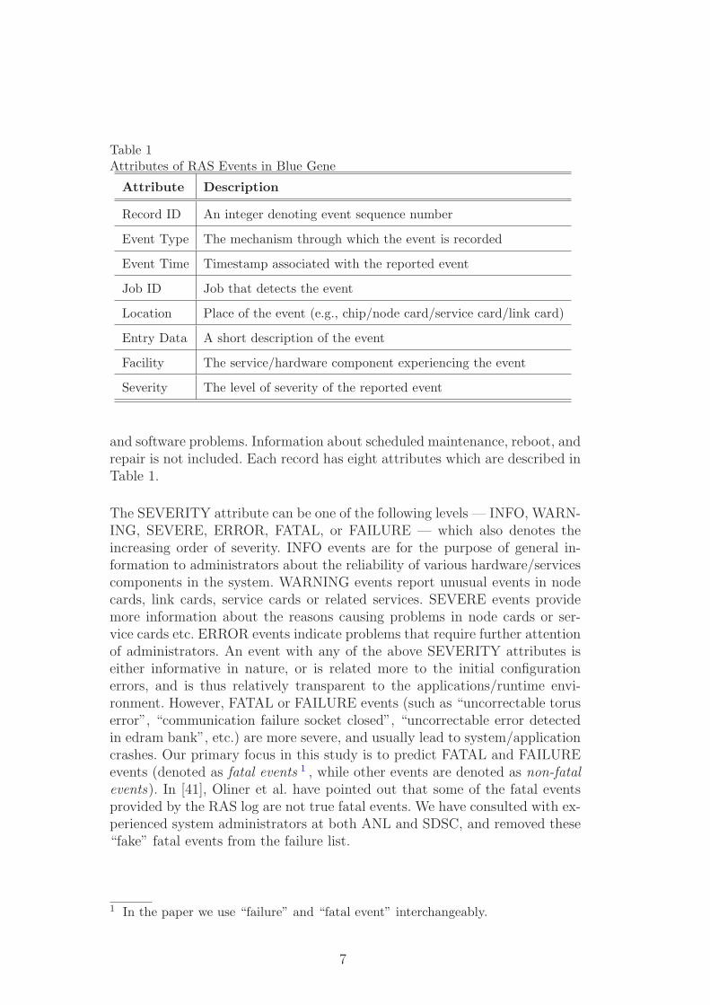
Table 1Attributes of RAS Events in Blue Gene

Attribute Description

Record ID An integer denoting event sequence number

Event Type The mechanism through which the event is recorded

Event Time Timestamp associated with the reported event

Job ID Job that detects the event

Location Place of the event (e.g., chip/node card/service card/link card)

Entry Data A short description of the event

Facility The service/hardware component experiencing the event

Severity The level of severity of the reported event

and software problems. Information about scheduled maintenance, reboot, andrepair is not included. Each record has eight attributes which are described inTable 1.

The SEVERITY attribute can be one of the following levels — INFO, WARN-ING, SEVERE, ERROR, FATAL, or FAILURE — which also denotes theincreasing order of severity. INFO events are for the purpose of general in-formation to administrators about the reliability of various hardware/servicescomponents in the system. WARNING events report unusual events in nodecards, link cards, service cards or related services. SEVERE events providemore information about the reasons causing problems in node cards or ser-vice cards etc. ERROR events indicate problems that require further attentionof administrators. An event with any of the above SEVERITY attributes iseither informative in nature, or is related more to the initial configurationerrors, and is thus relatively transparent to the applications/runtime envi-ronment. However, FATAL or FAILURE events (such as “uncorrectable toruserror”, “communication failure socket closed”, “uncorrectable error detectedin edram bank”, etc.) are more severe, and usually lead to system/applicationcrashes. Our primary focus in this study is to predict FATAL and FAILUREevents (denoted as fatal events 1 , while other events are denoted as non-fatalevents). In [41], Oliner et al. have pointed out that some of the fatal eventsprovided by the RAS log are not true fatal events. We have consulted with ex-perienced system administrators at both ANL and SDSC, and removed these“fake” fatal events from the failure list.

1 In the paper we use “failure” and “fatal event” interchangeably.

7

Table 2Log Description

Log Period Weeks Event No. Log Size

ANL BGL Jan. 21, 2005 - Jun. 19,2007 112 5,887,771 2.27 GB

SDSC BGL Dec. 6, 2004 - Jun. 11, 2007 132 517,247 463 MB

2.2 Test Logs

Two production Blue Gene/L systems are used in our experiments. One isat SDSC, which consists of three racks with 3,072 dual-core compute nodesand 384 I/O nodes. The configuration is chosen to support data-intensivecomputing. Each node consists of two PowerPC processors that run at 700MHz and share 512 MB of memory, giving an aggregate peak speed of 17.2teraflops and a total memory of 1.5 TB [31]. The other is at ANL, whichhas one rack with 1,024 dual-core compute nodes and 32 I/O nodes [32]. Theaggregate peak performance is of 5.7 teraflops, with a total memory of 500gigabytes. Both systems are mainly used for scientific computing. Table 2summarizes the RAS logs used in our experiments.

The log from ANL has much more number of records, although the systemhas only one rack of nodes. This is due to a large quantity of error checkingmessages produced at the ANL site. For example, during the 50th week of theANL’s log (between January 6 and January 13, 2006), there were over 1.15million of machine checking information messages generated. System admin-istrators at ANL ran diagnostics more frequently to cull out bad hardwarefaster, without applications seeing it.

3 Data Preprocessing

Raw logs generally contain many repeated or redundant information. This isbecause each computer chip runs a polling agent to collect the errors reportedby the chip. As each job is assigned to multiple computer chips, any failure ofthe job will get reported multiple places — once from each of the assigned com-puter chips. Thus multiple components may report the same failure. Also, thelogging mechanism records the events at a very fine granularity (e.g., in mil-lisecond), but the recorded event time is generally in seconds or minutes, thusleading to multiple entries of an event with the same time stamp. Therefore,before a RAS log can be used for failure prediction, it needs to be processedto identify unique RAS events.

As shown in Figure 1, data preprocessing mainly consists of two components:

8

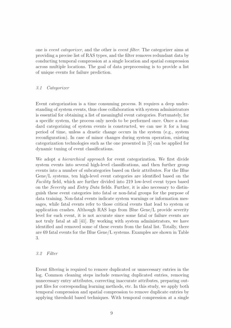
one is event categorizer, and the other is event filter. The categorizer aims atproviding a precise list of RAS types, and the filter removes redundant data byconducting temporal compression at a single location and spatial compressionacross multiple locations. The goal of data preprocessing is to provide a listof unique events for failure prediction.

3.1 Categorizer

Event categorization is a time consuming process. It requires a deep under-standing of system events, thus close collaboration with system administratorsis essential for obtaining a list of meaningful event categories. Fortunately, fora specific system, the process only needs to be performed once. Once a stan-dard categorizing of system events is constructed, we can use it for a longperiod of time, unless a drastic change occurs in the system (e.g., systemreconfiguration). In case of minor changes during system operation, existingcategorization technologies such as the one presented in [5] can be applied fordynamic tuning of event classifications.

We adopt a hierarchical approach for event categorization. We first dividesystem events into several high-level classifications, and then further groupevents into a number of subcategories based on their attributes. For the BlueGene/L systems, ten high-level event categories are identified based on theFacility field, which are further divided into 219 low-level event types basedon the Severity and Entry Data fields. Further, it is also necessary to distin-guish these event categories into fatal or non-fatal groups for the purpose ofdata training. Non-fatal events indicate system warnings or information mes-sages, while fatal events refer to those critical events that lead to system orapplication crashes. Although RAS logs from Blue Gene/L provide severitylevel for each event, it is not accurate since some fatal or failure events arenot truly fatal at all [41]. By working with system administrators, we haveidentified and removed some of these events from the fatal list. Totally, thereare 69 fatal events for the Blue Gene/L systems. Examples are shown in Table3.

3.2 Filter

Event filtering is required to remove duplicated or unnecessary entries in thelog. Common cleaning steps include removing duplicated entries, removingunnecessary entry attributes, correcting inaccurate attributes, preparing out-put files for corresponding learning methods, etc. In this study, we apply bothtemporal compression and spatial compression to remove duplicate entries byapplying threshold based techniques. With temporal compression at a single

9

Table 3Event Categories in Blue Gene/L

Main Examples No. of Fatal No. of Non-Fatal

Category Categories Categories

APP Load Program failure 10 7

function call failure

BGLMASTER segmentation failure 2 2

BGLMaster restart info

CMCS CMCS command info 0 4

CMCS exit info

DISCOVERY nodecard communication warning 0 24

servicecard read error

HARDWARE midplane service warning 1 12

KERNEL broadcast failure 46 90

cache failure

cpu failure

node map file error

LINKCARD linkcard failure 1 0

MMCS control network MMCS error 0 5

MONITOR node card temperature error 9 5

SERV NET system operation error 0 1

TOTAL 69 150

location, events from the same location with identical values in the Job ID andLocation fields are coalesced into a single entry, if reported within a predefinedtime duration. With spatial compression across multiple locations, we removethose entries that are close to each other within a predefined time duration,with the same Entry Date and Job ID, but from different locations.

How to decide an optimal threshold for filtering is still an open question. In thisstudy, we adopt an iterative approach [42,43]. We first set the threshold to avery small number, and then gradually increase the number. The search stopswhen there is no significant change with respect to compression rate. Table 4presents the numbers of events after applying different thresholds, where weseparate the numbers according to the high-level event categories. The columnwhere threshold is set to zero denotes the raw logs before any compression.

10

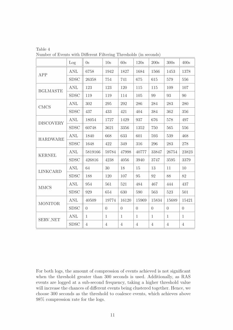
Table 4Number of Events with Different Filtering Thresholds (in seconds)

Log 0s 10s 60s 120s 200s 300s 400s

APPANL 6758 1942 1827 1684 1566 1453 1378

SDSC 26358 754 741 675 615 579 556

BGLMASTEANL 123 123 120 115 115 109 107

SDSC 119 119 114 105 99 93 90

CMCSANL 302 295 292 286 284 283 280

SDSC 437 433 421 404 384 362 356

DISCOVERYANL 18054 1727 1429 937 676 578 497

SDSC 60748 3621 3356 1352 750 565 556

HARDWAREANL 1840 668 633 601 593 539 468

SDSC 1648 422 349 316 296 283 278

KERNELANL 5819166 59784 47998 40777 33847 26754 23823

SDSC 426816 4238 4056 3940 3747 3595 3379

LINKCARDANL 64 30 18 15 13 11 10

SDSC 188 120 107 95 92 88 82

MMCSANL 954 561 521 484 467 444 437

SDSC 929 654 630 590 563 523 501

MONITORANL 40509 19774 16120 15969 15834 15689 15421

SDSC 0 0 0 0 0 0 0

SERV NETANL 1 1 1 1 1 1 1

SDSC 4 4 4 4 4 4 4

For both logs, the amount of compression of events achieved is not significantwhen the threshold greater than 300 seconds is used. Additionally, as RASevents are logged at a sub-second frequency, taking a higher threshold valuewill increase the chances of different events being clustered together. Hence, wechoose 300 seconds as the threshold to coalesce events, which achieves above98% compression rate for the logs.

11

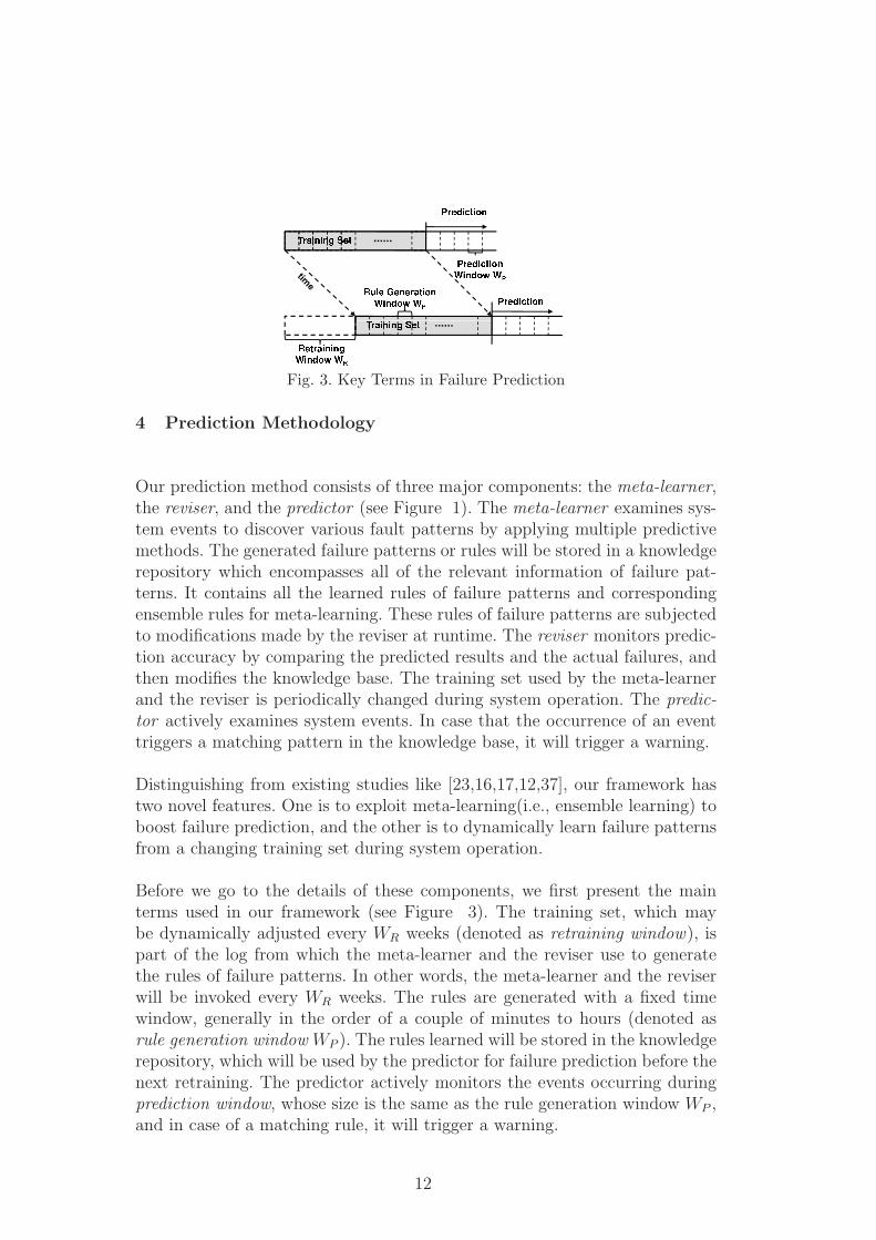
Fig. 3. Key Terms in Failure Prediction

4 Prediction Methodology

Our prediction method consists of three major components: the meta-learner,the reviser, and the predictor (see Figure 1). The meta-learner examines sys-tem events to discover various fault patterns by applying multiple predictivemethods. The generated failure patterns or rules will be stored in a knowledgerepository which encompasses all of the relevant information of failure pat-terns. It contains all the learned rules of failure patterns and correspondingensemble rules for meta-learning. These rules of failure patterns are subjectedto modifications made by the reviser at runtime. The reviser monitors predic-tion accuracy by comparing the predicted results and the actual failures, andthen modifies the knowledge base. The training set used by the meta-learnerand the reviser is periodically changed during system operation. The predic-tor actively examines system events. In case that the occurrence of an eventtriggers a matching pattern in the knowledge base, it will trigger a warning.

Distinguishing from existing studies like [23,16,17,12,37], our framework hastwo novel features. One is to exploit meta-learning(i.e., ensemble learning) toboost failure prediction, and the other is to dynamically learn failure patternsfrom a changing training set during system operation.

Before we go to the details of these components, we first present the mainterms used in our framework (see Figure 3). The training set, which maybe dynamically adjusted every WR weeks (denoted as retraining window), ispart of the log from which the meta-learner and the reviser use to generatethe rules of failure patterns. In other words, the meta-learner and the reviserwill be invoked every WR weeks. The rules are generated with a fixed timewindow, generally in the order of a couple of minutes to hours (denoted asrule generation window WP ). The rules learned will be stored in the knowledgerepository, which will be used by the predictor for failure prediction before thenext retraining. The predictor actively monitors the events occurring duringprediction window, whose size is the same as the rule generation window WP ,and in case of a matching rule, it will trigger a warning.

12

4.1 Meta-learner

The meta-learner focuses on revealing and learning the cause-and-effect rela-tions of system events by applying data mining techniques. Data mining, orknowledge discovery, is a computer-assisted process of searching and analyz-ing data sets for hidden patterns [11]. Meta-learning, also known as ensemble-learning, can be loosely defined as learning from learned knowledge [21]. Itemphasizes on combining different individual models (denoted as base learn-ers) to boost overall predictive effectiveness.

In this study, we choose three widely-used predictive methods, namely as-sociation rule based method [28,23], statistical rule based method [16], andprobability distribution based method [4], as our base learners. The meta-learner intends to identify a preferable combination of these base learners. Inthe following, we first describe the base learners, followed by presenting ourmeta-learning method. Note that other base methods can be easily incorpo-rated.

Base Learners. The first base learner is based on association rules. It ex-amines causal correlations between non-fatal and fatal events by buildingassociation rules. In general, an association rule is in the form X → Y , wherethe rule body X and Y are subsets of an event set. It states that a transactionthat contains the items in X are likely to contain the items in Y . Associationrules are characterized by two measures: support which measures the percent-age of transactions that contain both items X and Y , and confidence whichmeasures the percentage of item sets containing the items X that also containthe items Y . The problem of mining association rules consists of generating allthe association rules from a set of items that have both support and confidencegreater than the user-defined thresholds. Given that failure is rare event, lowvalues of support and confidence are set for the purpose of capturing infrequentevents.

On the training set, for each fatal event, we identify the set of non-fatal eventspreceding it within the rule generation window WP . The set, including the fatalevent and their precursor nonfatal events, is called an event set. We then applythe standard association rule algorithm to build rule models for event sets thatare above the minimum support and confidence. The association rules will bein the form of {e1, e2, · · · , ek} → f, confidence, where ei and ej (1 ≤ i, j ≤ k)are non-fatal events, f is a fatal event. For instance, two examples from theSDSC log are listed below:

networkWarningInterrupt, networkError → socketReadFailure: 1.0idoStartInfo, bglStartInfo → fsFailure: 0.79

Our second base learner emphasizes on discovering statistical characteristics,

13

Fig. 4. Temporal Correlations Among Fatal Events.

0 2 4 6 8 10 12

x 105

0

0.1

0.2

0.3

0.4

0.5

0.6

0.7

0.8

0.9

1

Inter−arrival Time between Fatal Events (in seconds)

Cum

ulat

ive

prob

abili

ty

ANL CDF_ANL_WeibullSDSC CDF_SDSC_Weibull

Fig. 5. Cumulative Distribution Functions (CDFs) of Fatal Events. The thin curvesrepresent the actual fatal events, while the thick curves model the Weibull distri-butions of the events.

i.e., how often and with what probability will the occurrence of one failureinfluence subsequent failures, among fatal events and then using the obtainedstatistical rules for failure prediction. It is denoted as statistical based method.Studies have shown that temporal correlations among fatal events are commonin large-scale systems [4,16,37]. Figure 4 plots fatal events per day occurred atANL and SDSC. We can observe that a significant number of failures happenin close proximity, and our further analysis indicates that network and I/Ostream related failures form a majority of such failures.

Specifically, on the training set, we calculate the probability of k failures oc-curred within the rule generation window WP . If the probability is larger thana user-defined threshold, then a statistic rule is generated, along with its prob-ability value. As an example, we have discovered that for both logs, if fourfailures occur within 300 seconds, then the probability of another failure is99%.

The third base learner is called probability based method. It generates probabil-ity distribution of fatal events and stores it for failure prediction. Different fromthe above two methods which attempt to discover short-term (e.g., in the or-der of minutes) correlations among events for failure prediction, this method

14

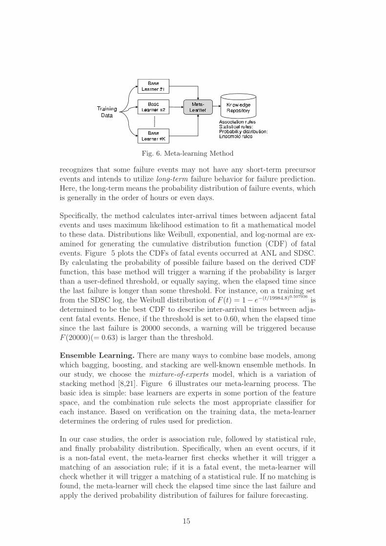
Fig. 6. Meta-learning Method

recognizes that some failure events may not have any short-term precursorevents and intends to utilize long-term failure behavior for failure prediction.Here, the long-term means the probability distribution of failure events, whichis generally in the order of hours or even days.

Specifically, the method calculates inter-arrival times between adjacent fatalevents and uses maximum likelihood estimation to fit a mathematical modelto these data. Distributions like Weibull, exponential, and log-normal are ex-amined for generating the cumulative distribution function (CDF) of fatalevents. Figure 5 plots the CDFs of fatal events occurred at ANL and SDSC.By calculating the probability of possible failure based on the derived CDFfunction, this base method will trigger a warning if the probability is largerthan a user-defined threshold, or equally saying, when the elapsed time sincethe last failure is longer than some threshold. For instance, on a training setfrom the SDSC log, the Weibull distribution of F (t) = 1− e−(t/19984.8)0.507936

isdetermined to be the best CDF to describe inter-arrival times between adja-cent fatal events. Hence, if the threshold is set to 0.60, when the elapsed timesince the last failure is 20000 seconds, a warning will be triggered becauseF (20000)(= 0.63) is larger than the threshold.

Ensemble Learning. There are many ways to combine base models, amongwhich bagging, boosting, and stacking are well-known ensemble methods. Inour study, we choose the mixture-of-experts model, which is a variation ofstacking method [8,21]. Figure 6 illustrates our meta-learning process. Thebasic idea is simple: base learners are experts in some portion of the featurespace, and the combination rule selects the most appropriate classifier foreach instance. Based on verification on the training data, the meta-learnerdetermines the ordering of rules used for prediction.

In our case studies, the order is association rule, followed by statistical rule,and finally probability distribution. Specifically, when an event occurs, if itis a non-fatal event, the meta-learner first checks whether it will trigger amatching of an association rule; if it is a fatal event, the meta-learner willcheck whether it will trigger a matching of a statistical rule. If no matching isfound, the meta-learner will check the elapsed time since the last failure andapply the derived probability distribution of failures for failure forecasting.

15

4.2 Reviser

The reviser is responsible for modifying the candidate rules generated by themeta-learner via monitoring the actual observations and the predicted results.This is to ensure the effectiveness of the learned rules in the knowledge repos-itory. As mentioned earlier, in order to capture infrequent items, the param-eters used in the base learners may be adopted without much considerationregarding their effectiveness, thereby probably resulting in some bad rules.Thus, the reviser checks each rule in the knowledge repository by applyingthe ROC (Receiver Operating Characteristic) analysis [11]. It enables us toselect optimal models and discard suboptimal ones independently from theclass distribution. The reviser will examine each rule and only keep the ruleswhich can provide satisfactory accuracy [9]. The detailed method is shown inAlgorithm 1.

Algorithm 1 The Reviser

For each rule r generated by the meta-learner:(1) Count its true positives TP , false positives FP , and false negatives FN

on the training data;(2) Calculate two metrics m1(r) and m2(r):

m1(r) =TP

TP + FP

,m2(r) =TP

TP + FN

;

(3) Calculate ROC(r):

ROC(r) =√

m1(r)2 + m2(r)2;

(4) Keep the rule if its ROC value is larger than a predefined thresholdMinROC; otherwise, discard the rule.

4.3 Predictor

The predictor actively monitors system events and triggers a warning whena rule is observed within the prediction window WP . In order to be used foronline forecasting, an event-driven method is adopted for its design [9]. Thatis, the predictor triggers a warning on the occurrence of events.

The detailed method is presented in Algorithm 2. The predictor maintainsthree event lists. One is called F − List which records a list of triggeringevents for each failure event. The second is called E − List which tracks alist of failure events that may be triggered by each event (fatal or non-fatal).The third is to keep the most recent events occurred within WP . Upon an

16

occurrence of an event e, the predictor appends the event into the third list(Step 1), and then goes through its E − List to find out all possible failuresthat may be triggered by its occurrence (Step 2). For each possible failuref i, the predictor checks its F − list to see whether a cause-and-effect rule ismatched in the knowledge repository (Step 3 and 4).

Algorithm 2 The Predictor

First, it creates two lists based on the learned rules:

F − List = {fi ⇐ {ei1, ei2, · · · , eik} : 1 ≤ i ≤ Nf}

E − List = {ej ⇒ {fj1, fj2, · · · , fjl} : 1 ≤ j ≤ Ne}

where fi is a fatal event and ei is a fatal or non-fatal event, Nf is numberof fatal events, and Ne is number of any events. During operating, when anevent e occurs:(1) Append e into the monitoring event set E = {e1, e2, · · · , en, e} where

the events are sorted in an increasing order of their occurrence times,remove ei if its occurrence time is more than WP before the occurrencetime of e, i.e., keep the most recent events occurred within WP

(2) Go through the E-List of e, obtain the potential failures that may betriggered by e: {f 1, f 2, · · · , fk}

(3) For each potential failure f i, go through its F-List: f i ⇐{ei

i1, eii2, · · · , e

iik}

(4) If {eii1, e

ii2, · · · , e

iik} ⊆ E, then produce a warning that the failure f i

may occur within the time of WP .

5 Experiments

To evaluate the effectiveness of the proposed framework, we use the realRAS logs collected from the production systems at ANL and SDSC (see Ta-ble 2). Further, to comprehensively examine the framework, our experimentsare structured to answer the key questions listed in Section 1.

5.1 Evaluation Metrics

Two metrics are used to measure prediction accuracy:

(1) Precision is defined as the proportion of correct predictions to all the

17

predictions made.

precision =Tp

Tp + Fp

(2) Recall is defined as the proportion of correct predictions to the numberof failures.

recall =Tp

Tp + Fn

Here, Tp is number of correct predictions (i.e., true positives), Fp is numberof false alarms (i.e., false positives), and Fn is number of missed failures (i.e.,false negatives). Obviously, a good prediction engine should achieve a highvalue (closer to 1.0) for both metrics. We note that these metrics are also usedby the reviser to determine whether a rule is effective or not (see Algorithm1).

5.2 Results

In our experiments, the training set is initially set to six months, which willbe dynamically adjusted during operation. The default retraining window WR

is four weeks, and the default prediction window WP , also the rule generationwindow, is 300 seconds.

The minimum support and confidence values for association rules are setto 0.01 and 0.1 respectively. The low values are chosen for the purpose ofcapturing infrequent events. The rules that are not good will be removed bythe reviser. There are three other parameters used by our framework, namelyMinROC for the reviser, and the thresholds for statistical rule based learnerand probability distribution based learner. In our experiments, MinROC isset to 0.7, and the thresholds for statistical rules and probability distributionbased learner are set to 0.8 and 0.6 respectively. Choosing optimal values forthese parameters is difficult, and often experimental determination might bethe only viable option. We have tested different values, from a low value like0.1 to a high value like 0.9, and found that these values can yield the bestprediction accuracy for both logs. In general, low values for these parametersresult in more failure rules and thus better failure coverage, at the expense ofintroducing more false alarms.

5.2.1 Q1: How Much Improvement Is Achieved by the Meta-learning?

In this set of experiments, we compare prediction results by using static meta-learner as against individual base learners (i.e., association rule, statistical

18

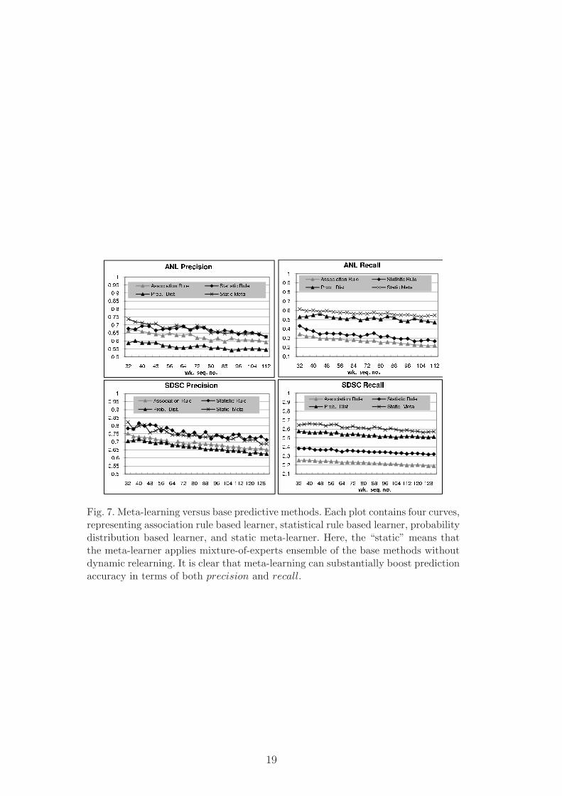
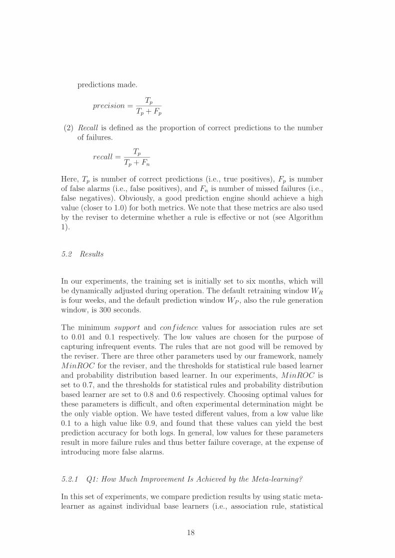
Fig. 7. Meta-learning versus base predictive methods. Each plot contains four curves,representing association rule based learner, statistical rule based learner, probabilitydistribution based learner, and static meta-learner. Here, the “static” means thatthe meta-learner applies mixture-of-experts ensemble of the base methods withoutdynamic relearning. It is clear that meta-learning can substantially boost predictionaccuracy in terms of both precision and recall.

19

rule, and probability distribution). Here, the “static” means that the meta-learner simply applies mixture-of-experts ensemble of the base methods, with-out dynamic training, retraining and revising. Hence, for both logs, the firstsix months are used as the training set, and the remaining parts are for test-ing. The results are shown in Figure 7, where the x-axis shows the sequencenumber of the week.

First, both precision and recall decrease as the time goes by, no matter whichmethod is used. The reason is that all these methods are based on a staticapproach, meaning that they learn the rules on the six-month training setand then use these rules for prediction on the rest of the logs. The rules maywell capture failure patterns at the beginning. However, system behavior isdynamically changing. As a result, the established rules become outdated,thereby resulting in lower prediction accuracy as the time goes by.

We make several interesting observations regarding each base method. First,statistical rule base method provides a reasonably good result for precision;however, it results in a low value for recall. It suggests that this methodis only good at discovering certain types of failures which exhibit temporalcorrelations. Second, association rule base method has the worse results interms of recall. This is mainly due to the fact that while this method wellcaptures causal correlation between non-fatal and fatal events, it is limited bythe proportion of fatal events without any precursor warnings (e.g., low recall

values). Our analysis shows that for both logs, there are a large portion offatal events (up to 75%) which are not preceded by any precursor non-fatalevents. Third, the recall results provided by probability distribution basedmethod are quite good (e.g., higher than 0.5 for both logs). Nevertheless,it can introduce many false alarms. The problem of probability distributionbased method is that it cannot pinpoint the occurrence times of the failures,thereby giving many false alarms once the elapsed time since the last failureis large enough.

A Venn diagram of these base learners is presented in Figure 8. It shows thenumbers of fatal events predicted by these base learners between the 44th and48th week of the SDSC log. In total, there are 156 fatal events during thisperiod, and 67 of them are captured by multiple base learners. The coverageof each base learner is as follows: association rule based learner 23.7% (37 fatalevents), statistical rule based learner 37.2% (58 fatal events), and probabilitydistribution based learner 56.4% (88 fatal events). The diagram clearly showsthat it is improper to expect a single method to capture all of failures alone.

Observation #1: In a large-scale system, there are numerous failure patternsin general; thus a single base learner is unlikely to capture all of them alone.

Meta-learning can substantially improve recall, indicating that meta-learning

20

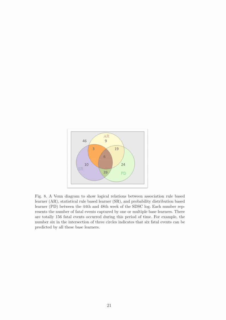
Fig. 8. A Venn diagram to show logical relations between association rule basedlearner (AR), statistical rule based learner (SR), and probability distribution basedlearner (PD) between the 44th and 48th week of the SDSC log. Each number rep-resents the number of fatal events captured by one or multiple base learners. Thereare totally 156 fatal events occurred during this period of time. For example, thenumber six in the intersection of three circles indicates that six fatal events can bepredicted by all these base learners.

21

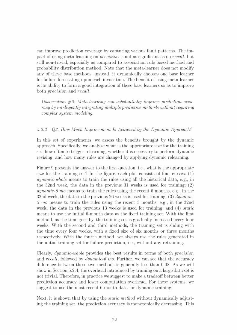
can improve prediction coverage by capturing various fault patterns. The im-pact of using meta-learning on precision is not as significant as on recall, butstill non-trivial, especially as compared to association rule based method andprobability distribution method. Note that the meta-learner does not modifyany of these base methods; instead, it dynamically chooses one base learnerfor failure forecasting upon each invocation. The benefit of using meta-learneris its ability to form a good integration of these base learners so as to improveboth precision and recall.

Observation #2: Meta-learning can substantially improve prediction accu-racy by intelligently integrating multiple predictive methods without requiringcomplex system modeling.

5.2.2 Q2: How Much Improvement Is Achieved by the Dynamic Approach?

In this set of experiments, we assess the benefits brought by the dynamicapproach. Specifically, we analyze what is the appropriate size for the trainingset, how often to trigger relearning, whether it is necessary to perform dynamicrevising, and how many rules are changed by applying dynamic relearning.

Figure 9 presents the answer to the first question, i.e., what is the appropriatesize for the training set? In the figure, each plot consists of four curves: (1)dynamic-whole means to train the rules using all the historical data, e.g., inthe 32nd week, the data in the previous 31 weeks is used for training; (2)dynamic-6 mo means to train the rules using the recent 6 months, e.g., in the32nd week, the data in the previous 26 weeks is used for training; (3) dynamic-3 mo means to train the rules using the recent 3 months, e.g., in the 32ndweek, the data in the previous 13 weeks is used for training; and (4) staticmeans to use the initial 6-month data as the fixed training set. With the firstmethod, as the time goes by, the training set is gradually increased every fourweeks. With the second and third methods, the training set is sliding withthe time every four weeks, with a fixed size of six months or three monthsrespectively. With the fourth method, we always use the rules generated inthe initial training set for failure prediction, i.e., without any retraining.

Clearly, dynamic-whole provides the best results in terms of both precision

and recall, followed by dynamic-6 mo. Further, we can see that the accuracydifference between these two methods is generally less than 0.08. As we willshow in Section 5.2.4, the overhead introduced by training on a large data set isnot trivial. Therefore, in practice we suggest to make a tradeoff between betterprediction accuracy and lower computation overhead. For these systems, wesuggest to use the most recent 6-month data for dynamic training.

Next, it is shown that by using the static method without dynamically adjust-ing the training set, the prediction accuracy is monotonically decreasing. This

22

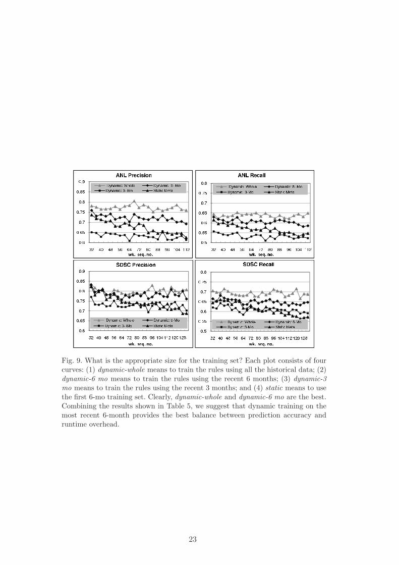
Fig. 9. What is the appropriate size for the training set? Each plot consists of fourcurves: (1) dynamic-whole means to train the rules using all the historical data; (2)dynamic-6 mo means to train the rules using the recent 6 months; (3) dynamic-3mo means to train the rules using the recent 3 months; and (4) static means to usethe first 6-mo training set. Clearly, dynamic-whole and dynamic-6 mo are the best.Combining the results shown in Table 5, we suggest that dynamic training on themost recent 6-month provides the best balance between prediction accuracy andruntime overhead.

23

is reasonable as the fixed rule set learned by static meta-learner is unable toadapt to new changes/reconfigurations occurring in the system.

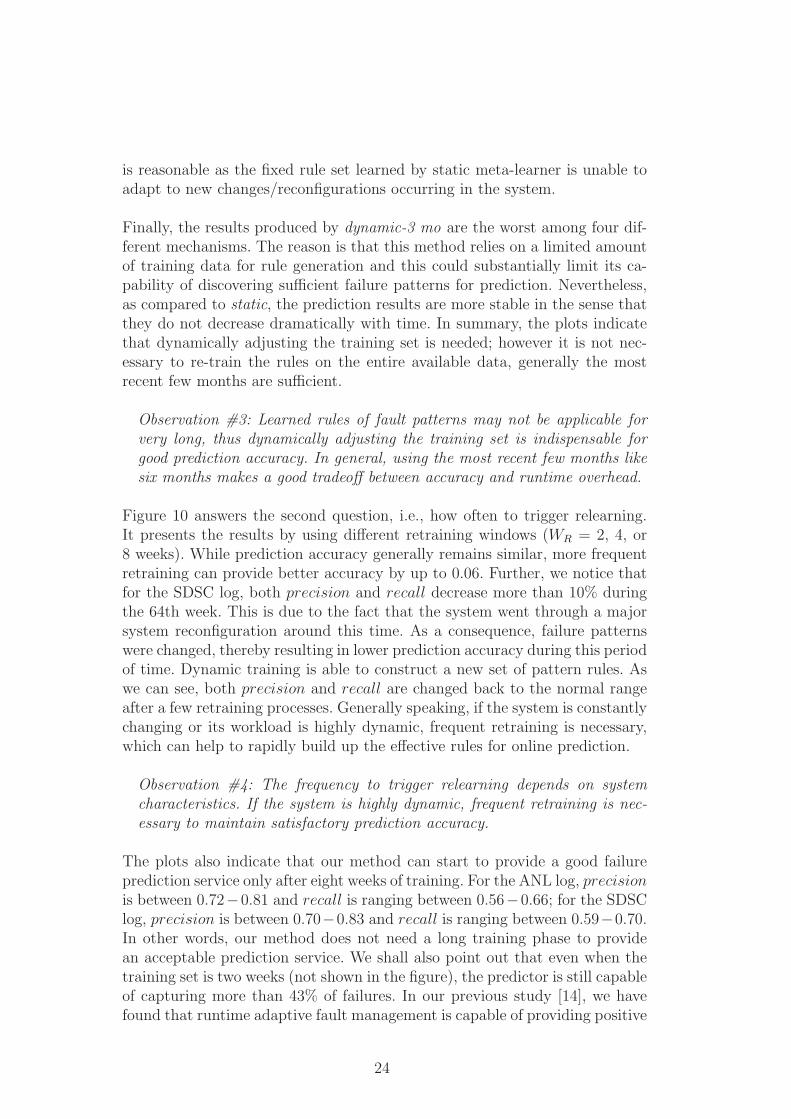
Finally, the results produced by dynamic-3 mo are the worst among four dif-ferent mechanisms. The reason is that this method relies on a limited amountof training data for rule generation and this could substantially limit its ca-pability of discovering sufficient failure patterns for prediction. Nevertheless,as compared to static, the prediction results are more stable in the sense thatthey do not decrease dramatically with time. In summary, the plots indicatethat dynamically adjusting the training set is needed; however it is not nec-essary to re-train the rules on the entire available data, generally the mostrecent few months are sufficient.

Observation #3: Learned rules of fault patterns may not be applicable forvery long, thus dynamically adjusting the training set is indispensable forgood prediction accuracy. In general, using the most recent few months likesix months makes a good tradeoff between accuracy and runtime overhead.

Figure 10 answers the second question, i.e., how often to trigger relearning.It presents the results by using different retraining windows (WR = 2, 4, or8 weeks). While prediction accuracy generally remains similar, more frequentretraining can provide better accuracy by up to 0.06. Further, we notice thatfor the SDSC log, both precision and recall decrease more than 10% duringthe 64th week. This is due to the fact that the system went through a majorsystem reconfiguration around this time. As a consequence, failure patternswere changed, thereby resulting in lower prediction accuracy during this periodof time. Dynamic training is able to construct a new set of pattern rules. Aswe can see, both precision and recall are changed back to the normal rangeafter a few retraining processes. Generally speaking, if the system is constantlychanging or its workload is highly dynamic, frequent retraining is necessary,which can help to rapidly build up the effective rules for online prediction.

Observation #4: The frequency to trigger relearning depends on systemcharacteristics. If the system is highly dynamic, frequent retraining is nec-essary to maintain satisfactory prediction accuracy.

The plots also indicate that our method can start to provide a good failureprediction service only after eight weeks of training. For the ANL log, precisionis between 0.72−0.81 and recall is ranging between 0.56−0.66; for the SDSClog, precision is between 0.70−0.83 and recall is ranging between 0.59−0.70.In other words, our method does not need a long training phase to providean acceptable prediction service. We shall also point out that even when thetraining set is two weeks (not shown in the figure), the predictor is still capableof capturing more than 43% of failures. In our previous study [14], we havefound that runtime adaptive fault management is capable of providing positive

24

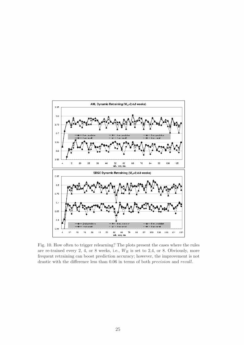
Fig. 10. How often to trigger relearning? The plots present the cases where the rulesare re-trained every 2, 4, or 8 weeks, i.e., WR is set to 2,4, or 8. Obviously, morefrequent retraining can boost prediction accuracy; however, the improvement is notdrastic with the difference less than 0.06 in terms of both precision and recall.

25

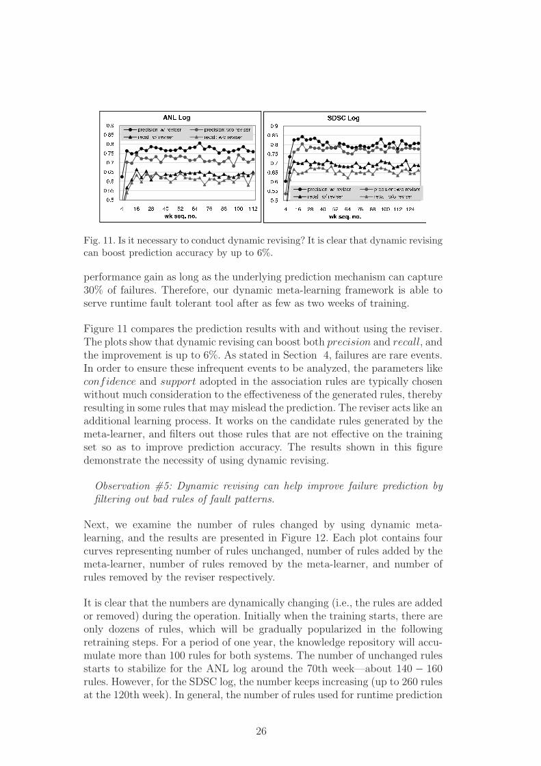
Fig. 11. Is it necessary to conduct dynamic revising? It is clear that dynamic revisingcan boost prediction accuracy by up to 6%.

performance gain as long as the underlying prediction mechanism can capture30% of failures. Therefore, our dynamic meta-learning framework is able toserve runtime fault tolerant tool after as few as two weeks of training.

Figure 11 compares the prediction results with and without using the reviser.The plots show that dynamic revising can boost both precision and recall, andthe improvement is up to 6%. As stated in Section 4, failures are rare events.In order to ensure these infrequent events to be analyzed, the parameters likeconfidence and support adopted in the association rules are typically chosenwithout much consideration to the effectiveness of the generated rules, therebyresulting in some rules that may mislead the prediction. The reviser acts like anadditional learning process. It works on the candidate rules generated by themeta-learner, and filters out those rules that are not effective on the trainingset so as to improve prediction accuracy. The results shown in this figuredemonstrate the necessity of using dynamic revising.

Observation #5: Dynamic revising can help improve failure prediction byfiltering out bad rules of fault patterns.

Next, we examine the number of rules changed by using dynamic meta-learning, and the results are presented in Figure 12. Each plot contains fourcurves representing number of rules unchanged, number of rules added by themeta-learner, number of rules removed by the meta-learner, and number ofrules removed by the reviser respectively.

It is clear that the numbers are dynamically changing (i.e., the rules are addedor removed) during the operation. Initially when the training starts, there areonly dozens of rules, which will be gradually popularized in the followingretraining steps. For a period of one year, the knowledge repository will accu-mulate more than 100 rules for both systems. The number of unchanged rulesstarts to stabilize for the ANL log around the 70th week—about 140 − 160rules. However, for the SDSC log, the number keeps increasing (up to 260 rulesat the 120th week). In general, the number of rules used for runtime prediction

26

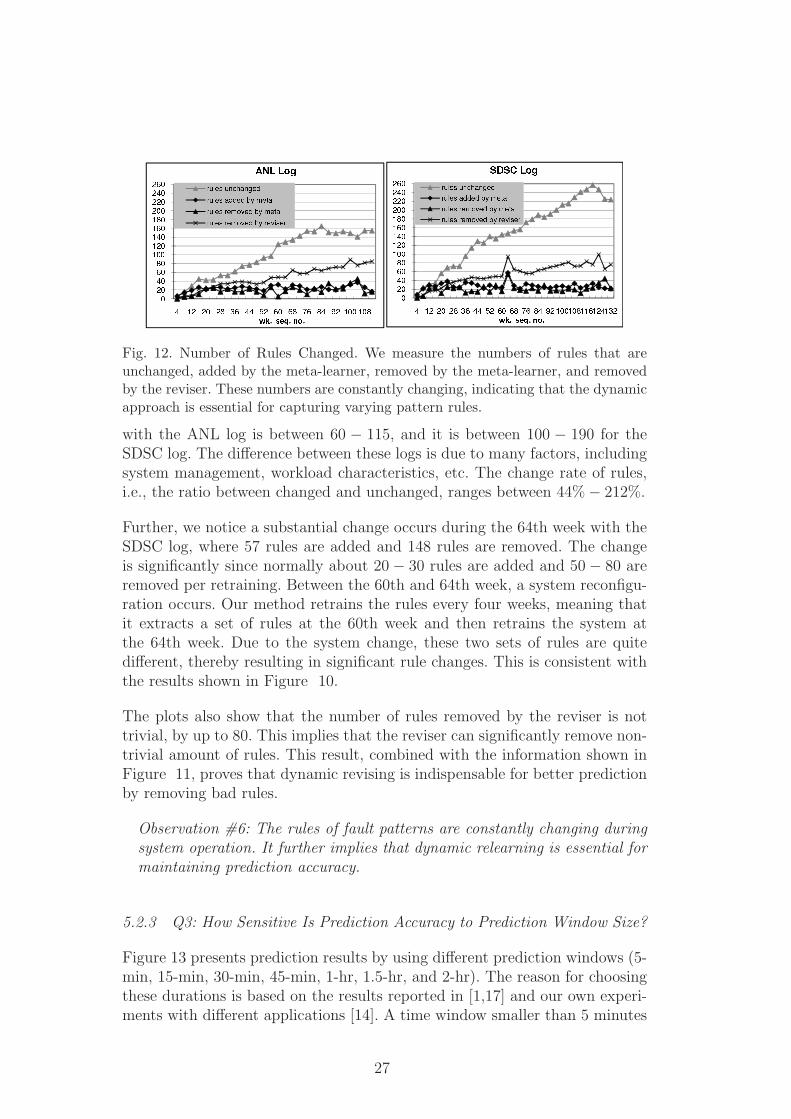
Fig. 12. Number of Rules Changed. We measure the numbers of rules that areunchanged, added by the meta-learner, removed by the meta-learner, and removedby the reviser. These numbers are constantly changing, indicating that the dynamicapproach is essential for capturing varying pattern rules.

with the ANL log is between 60 − 115, and it is between 100 − 190 for theSDSC log. The difference between these logs is due to many factors, includingsystem management, workload characteristics, etc. The change rate of rules,i.e., the ratio between changed and unchanged, ranges between 44% − 212%.

Further, we notice a substantial change occurs during the 64th week with theSDSC log, where 57 rules are added and 148 rules are removed. The changeis significantly since normally about 20 − 30 rules are added and 50 − 80 areremoved per retraining. Between the 60th and 64th week, a system reconfigu-ration occurs. Our method retrains the rules every four weeks, meaning thatit extracts a set of rules at the 60th week and then retrains the system atthe 64th week. Due to the system change, these two sets of rules are quitedifferent, thereby resulting in significant rule changes. This is consistent withthe results shown in Figure 10.

The plots also show that the number of rules removed by the reviser is nottrivial, by up to 80. This implies that the reviser can significantly remove non-trivial amount of rules. This result, combined with the information shown inFigure 11, proves that dynamic revising is indispensable for better predictionby removing bad rules.

Observation #6: The rules of fault patterns are constantly changing duringsystem operation. It further implies that dynamic relearning is essential formaintaining prediction accuracy.

5.2.3 Q3: How Sensitive Is Prediction Accuracy to Prediction Window Size?

Figure 13 presents prediction results by using different prediction windows (5-min, 15-min, 30-min, 45-min, 1-hr, 1.5-hr, and 2-hr). The reason for choosingthese durations is based on the results reported in [1,17] and our own experi-ments with different applications [14]. A time window smaller than 5 minutes

27

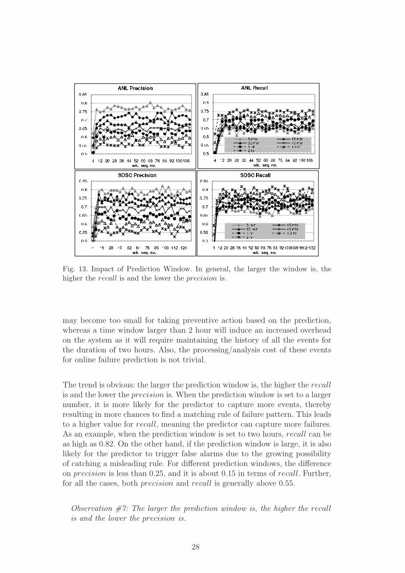
Fig. 13. Impact of Prediction Window. In general, the larger the window is, thehigher the recall is and the lower the precision is.

may become too small for taking preventive action based on the prediction,whereas a time window larger than 2 hour will induce an increased overheadon the system as it will require maintaining the history of all the events forthe duration of two hours. Also, the processing/analysis cost of these eventsfor online failure prediction is not trivial.

The trend is obvious: the larger the prediction window is, the higher the recall

is and the lower the precision is. When the prediction window is set to a largernumber, it is more likely for the predictor to capture more events, therebyresulting in more chances to find a matching rule of failure pattern. This leadsto a higher value for recall, meaning the predictor can capture more failures.As an example, when the prediction window is set to two hours, recall can beas high as 0.82. On the other hand, if the prediction window is large, it is alsolikely for the predictor to trigger false alarms due to the growing possibilityof catching a misleading rule. For different prediction windows, the differenceon precision is less than 0.25, and it is about 0.15 in terms of recall. Further,for all the cases, both precision and recall is generally above 0.55.

Observation #7: The larger the prediction window is, the higher the recall

is and the lower the precision is.

28

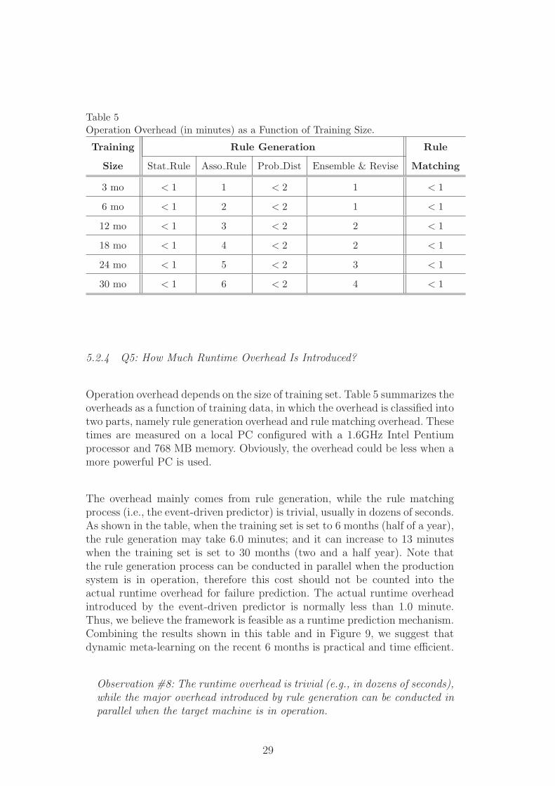
Table 5Operation Overhead (in minutes) as a Function of Training Size.

Training Rule Generation Rule

Size Stat Rule Asso Rule Prob Dist Ensemble & Revise Matching

3 mo < 1 1 < 2 1 < 1

6 mo < 1 2 < 2 1 < 1

12 mo < 1 3 < 2 2 < 1

18 mo < 1 4 < 2 2 < 1

24 mo < 1 5 < 2 3 < 1

30 mo < 1 6 < 2 4 < 1

5.2.4 Q5: How Much Runtime Overhead Is Introduced?

Operation overhead depends on the size of training set. Table 5 summarizes theoverheads as a function of training data, in which the overhead is classified intotwo parts, namely rule generation overhead and rule matching overhead. Thesetimes are measured on a local PC configured with a 1.6GHz Intel Pentiumprocessor and 768 MB memory. Obviously, the overhead could be less when amore powerful PC is used.

The overhead mainly comes from rule generation, while the rule matchingprocess (i.e., the event-driven predictor) is trivial, usually in dozens of seconds.As shown in the table, when the training set is set to 6 months (half of a year),the rule generation may take 6.0 minutes; and it can increase to 13 minuteswhen the training set is set to 30 months (two and a half year). Note thatthe rule generation process can be conducted in parallel when the productionsystem is in operation, therefore this cost should not be counted into theactual runtime overhead for failure prediction. The actual runtime overheadintroduced by the event-driven predictor is normally less than 1.0 minute.Thus, we believe the framework is feasible as a runtime prediction mechanism.Combining the results shown in this table and in Figure 9, we suggest thatdynamic meta-learning on the recent 6 months is practical and time efficient.

Observation #8: The runtime overhead is trivial (e.g., in dozens of seconds),while the major overhead introduced by rule generation can be conducted inparallel when the target machine is in operation.

29

6 Related Work

Recognizing the importance of fault tolerance, the community has paid muchattention to failure prediction. Exiting predictive approaches can be broadlyclassified as model-based or data-driven methods. Model-based approach de-rives a probabilistic or analytical model of the system and triggers a warningwhen a deviation from the model is detected [7,13,25]. Examples include anadaptive statistical data fitting method called MSET presented in [26], Semi-Markov reward models described in [34], and a naive Bayesian based modelto predict disk drive failures [12]. In large-scale systems, errors may propagatefrom one component to other component, which is commonly addressed by de-veloping fault propagation models (FPM) [35]. While model-based methods areeffective for forecasting some failures, they seem too complicated to be practicalfor failure prediction in large-scale systems composed of tens of thousands ofcomponents.

A data-driven method, such as using data mining techniques, attempts to learnfailure patterns from historical data for failure prediction, without construct-ing an accurate model ahead of time. These methods extract fault patternsfrom system normal behaviors, and detect abnormal observations based onthe learned knowledge without assuming a priori model ahead of time. Forexample, the group at the RAD laboratory has applied statistical learningtechniques for failure diagnosis in Internet services [27,33]. The SLIC (Sta-tistical Learning, Inference and Control) project at HP has explored similartechniques for automating fault management of IT systems [36]. Sahoo et al.have applied association rules to predict failure events in a 350-node IBMcluster [23]. In [16,17], Liang et al. have examined several data mining andmachine learning techniques for failure forecasting in a Blue Gene/L system.Other representative works include system log analysis [4,41] and a predictionframework for networked systems [37].

While this paper is built upon existing studies, it distinguishes from the abovestudies at several aspects. First, unlike existing studies focusing on one specificpredictive method, this paper presents a dynamic meta-learning framework todynamically integrate existing predictive methods for better prediction. Inthis study, we have examined three widely-used predictive methods, namelyassociation rule based learner [23,28], statistical rule based learner [16], andprobability distribution based learner [4] in the framework. We believe otherpredictive methods can be easily incorporated into our framework. Second,this study emphasizes dynamic training and learning, which is rarely exam-ined in the literature. By means of real system logs from production systems,we have demonstrated that dynamic relearning is essential to capture behav-ior changes during system operation. By examining our framework in variousways, we have shown that using the most recent few months like six months

30

makes a good tradeoff between accuracy and runtime overhead. Next, unlikeoffline log analysis studies, our prediction is event-driven, meaning that ourframework triggers a warning on the occurrence of events during system op-eration. An event-driven approach is well suited for online failure prediction.Last but not the least, in addition to presenting the key techniques for boost-ing prediction accuracy, we have also systematically analyzed our frameworkand answered several key questions commonly raised in failure prediction. Itprovides a deep insight into failure prediction in large-scale systems. To thebest of our knowledge, we are among the first to comprehensively evaluate theimpact of different factors in failure forecasting.

7 Summary

In this paper, we have presented a dynamic meta-learning prediction enginefor large-scale systems. Recognizing problems in failure prediction, our predic-tion mechanism relies on two key techniques to improve prediction accuracyin real systems. Meta-learning is applied to boost prediction accuracy by in-tegrating multiple predictive methods, while a dynamic approach is employedto train the rules of failure patterns at runtime. Our prediction mechanismdoes not require a long training phase by dynamically adjusting the trainingset during system operation. Further, it can adapt to system changes, evenafter a major system reconfiguration. Our case studies with real system logshave demonstrated its effectiveness with a good accuracy, e.g., capturing upto 82% of failures. The studies have also shown that the proposed mechanismis practical and well suited for forecasting failures in real systems.

Our study has some limitations that remain as our future work. First, in thecurrent design, the prediction window size is fixed. Our on-going work includesadaptively changing this window size such that the system can automaticallytune its size to reduce the training cost, without sacrificing the prediction accu-racy. Second, we plan to examine other data mining methods, such as decisiontree and neural network, to popularize our base learners. We will also investi-gate other ensemble learning techniques to improve the meta-learner. Finally,more case studies with a variety of HPC systems will be conducted. Althoughour case studies focus on the Blue Gene/L systems, we believe the proposedmechanism is applicable to other systems. For the systems that do not havean error checking and logging facility, the first step is to develop a monitor-ing tool which is capable of gathering fault-related information from varioussystem components and archive the information in a centralized repository.The proposed framework can be easily extended to these systems by linkingto their event repositories.

31

Acknowledgment

Zhiling Lan is supported in part by US National Science Foundation grantsCNS-0834514, CNS-0720549, CCF-0702737, and a TeraGrid Compute Alloca-tion. Susan Coghlan and Rajeev Thakur are supported by the Office of Ad-vanced Scientific Computing Research, Office of Science, U.S. Department ofEnergy, under Contract DE-AC02-06CH11357. We would like to thank JohnWhite at Revision3 Company and Eva Hocks at San Diego SupercomputerCenter for the discussion of the SDSC system log. Some preliminary resultsof this work were presented in [8,9].

References

[1] E. Elnozahy and J. Plank, Checkpointing for Peta-Scale Systems: A Look into theFuture of Practical Rollback-Recovery, IEEE Trans. on Dependable and SecureComputing, vol. 1(2), pp. 97-108, 2004.

[2] G. Hoffmann, F. Salfner, and M. Malek, Advanced Failure Prediction in ComplexSoftware Systems, Proc. of SRDS’04, 2004.

[3] A. Gara, M. Blumrich, D. Chen, G. Chiu, P. Coteus, M. Giampapa, R.Haring, P. Heidelberger, D. Hoenicke, G. Kopcsay, T. Liebsch, M. Ohmacht,B. Steinmacher-Burow, T. Takken, P. Vranas, Overview of the Blue Gene/LSystem Architecture, IBM J. Res. & Dev., vol. 49(2/3), 2005.

[4] B. Schroeder and G. Gibson, A Large-scale Study of Failures in High PerformanceComputing Systems, Proc. of DSN’06, 2006.

[5] W. Peng, T. Li and S. Ma, Mining Logs Files for Computing SystemManagement, Proc. of ICAC’05,2005.

[6] R. Gioiosa, J. Sancho, S. Jiang, F. Petrini, and K. Davis, TransparentIncremental Checkpointing at Kernel Level: A Foundation for Fault Tolerancefor Parallel Computers, Proc. of SC’05, 2005.

[7] A. Goyal, S. Lavenberg, and K. Trivedi, Probabilistic Modeling of ComputerSystem Availability, Annals of Operations Research, 1987.

[8] P. Gujrati, Y. Li, Z. Lan, R. Thakur, and J. White, A Meta-learning FailurePredictor for Blue Gene/L Systems, Proc. of ICPP’07, 2007.

[9] J. Gu, Z. Zheng, Z. Lan, J. White, E. Hocks, and B. Park, Dynamic Meta-Learning for Failure Prediction in Large-Scale Systems: A Case Study, Proc. ofICPP’08, 2008.

[10] Y. Zhang, M. Squillante, A. Sivasubramaniam and R. Sahoo, PerformanceImplications of Failures in Large-Scale Cluster Scheduling, Proc. of Workshopon Job Scheduling Strategies for Parallel Processing, 2004.

32

[11] J. Han and M. Kamber, Data Mining: Concepts and Techniques, 2nd Edition,Morgan Kaufmann, 2006.

[12] G. Hamerly and C. Elkan, Bayesian Approaches to Failure Prediction for DiskDrives, Proc. of ICML’01, 2001.

[13] J. Hellerstein, F. Zhang, and P. Shahabuddin, A Statistical Approachto Predictive Detection, Computer Networks: The International Journal ofComputer and Telecommunications Networking, 2001.

[14] Z. Lan and Y. Li, Adaptive Fault Management of Parallel Applications forHigh Performance Computing, IEEE Trans. on Computers, 57(12), pp. 1647-1660, 2008.

[15] Y. Li, Z. Lan, P. Gujrati, and X. Sun, Fault-Aware Runtime Strategies for HighPerformance Computing, IEEE Trans. on Parallel and Distributed Systems, vol.20(4), pp. 460-473, 2009.

[16] Y. Liang, Y. Zhang, A. Sivasubramaniam, M. Jette, and R. Sahoo, Blue Gene/LFailure Analysis and Models, Proc. of DSN’06, 2006.

[17] Y. Liang, Y. Zhang, H. Xiong and R. Shaoo, Failure Prediction in IBMBlueGene/L Event Logs, Proc. of ICDM’07, 2007.

[18] A. Oliner, L. Rudolph, and R. Sahoo, Cooperative Checkpointing Theory, Proc.of the International Parallel and Distributed Processing Symposium (IPDPS),2006.

[19] A. Oliner and J. Stearly, What Supercomputers Say: A Study of Five SystemLogs, Proc. of DSN’07, 2007.

[20] A. Oliner, R. Sahoo, J. Moreira, M. Gupta, and A. Sivasubramaniam, Fault-Aware Job Scheduling for Blue Gene/L Systems, Proc. of IPDPS’04, 2004.

[21] R. Polikar, Ensemble Based Systems in Decision Making, IEEE Circuits andSystems Magazine, vol.6(3), 2006.

[22] D. Reed, C. Lu, and C. Mendes, Big Systems and Big Reliability Challenges,Proc. of Parallel Computing, 2003.

[23] R. Sahoo, A. Oliner, I. Rish, M. Gupta, J. Moreira, and S. Ma, Critical EventPrediction for Proactive Management in Large-scale Computer Clusters, Proc.of SIGKDD’03, 2003.

[24] M. Schulz, G. Bronevetsky, R. Fernandes, D. Marques, K. Pingali, andP. Stodghill, Implementation and Evaluation of a Scalable Application-levelCheckpoint-Recovery Scheme for MPI Programs, Proc. of SC’04, 2004.

[25] K. Trivedi and K. Vaidyanathan, A Measurement-based Model for Estimationof Resource Exhaustion in Operational Software Systems, Proc. of ISSRE’99,1999.

[26] K. Vaidyanathan and K. Gross, MSET Performance Optimization for Detectionof Software Aging, Proc. of ISSRE, 2003.

33

[27] M. Chen, A. Zheng, J. Lloyd, M. Jordan, and E. Brewer, Failure DiagnosisUsing Decision Trees, Proc. of ICAC’04, 2004.

[28] R. Vilalta and S. Ma, Predicting Rare Events in Temporal Domains, Proc. ofICDM’02, 2002.

[29] C. Wang, F. Mueller, C. Engelmann and S. Scott, A Job Pause Service underLAM/MPI+BLCR for Transparent Fault Tolerance, Proc. of IPDPS’07, 2007.

[30] The TOP500 Supercomputer Site, available at http://www.top500.org/

[31] The Blue Gene System at SDSC, available athttp://www.sdsc.edu/us/resources/bluegene/

[32] The Blue Gene System at ANL, available at http://www.bgl.mcs.anl.gov/

[33] P. Bodik, G. Friedman, L. Biewald, H. Levine, G. Candea, K. Patel, G. Tolle,J. Hui, A. Fox, M. Jordan, and D. Patterson, Combining Visualization andStatistical Analysis to Improve Operator Confidence and Efficiency for FailureDetection and Localization, Proc. of The 2nd IEEE International Conference onAutonomic Computing (ICAC ’05), 2005.

[34] S. Garg, A. Puliafito, and K. Trivedi, Analysis of Software Rejuvenation UsingMarkov Regenerative Stochastic Petri Net, Proc. of 6th International Symposiumon Software Reliability Engineering, 1995.

[35] M. Steinder and A. Sethi, A Survey of Fault Localization Techniques inComputer Networks, Science of Computer Programming, vol. 53, 2004.

[36] I. Cohen and J. Chase, Correlating Instrumentation Data to System States: Abuilding Block for Automated Diagnosis and control, Proc. of OSDI’04, 2004.

[37] S. Fu and C. Xu, Exploring Event Correlation for Failure Prediction inCoalitions of Clusters, Proc. of SC’07, 2007.

[38] P. Hargrove and J. Duell, Berkeley Lab Checkpoint/Restart (BLCR) for LinuxClusters, Proc. of SciDAC 2006 (publication LBNL-60520), 2006.

[39] M. Joshi, R. Agarwal, and V. Kumar, Mining Needle in a Haystack: ClassifyingRare Classes via Two-phase Rule Induction, Proc. of SIGMOD’01, 2001.

[40] G. Weiss, Mining with Rarity: a Unifying Framework, ACM SIGKDDExplorations, vol. 6(1):719, 2004.

[41] A. Oliner and J. Stearley, What Supercomputers Say: A Study of Five SystemLogs, Proc. of the International Conference on Dependable Systems and Networks(DSN), 2007.

[42] J. Hansen and D. Siewiorek, Models for Time Coalescence in Event Logs, Proc.of Fault-Tolerant Computing (FTCS), 1992.

[43] M. Buckley and D. Siewiorek, Comparative Analysis of Event Tupling Schemes,Proc. of Fault-Tolerant Computing (FTCS), 1996.

34