a study of mhd and monte carlo simulations of high-current … · 2016-04-14 ·...
TRANSCRIPT

A Study of MHD and Monte Carlo
Simulations
of High-Current Plasma Beams in
Industrial Applications
by
Luping Zhang
A Thesis Submitted in Partial Fulfillment
of the Requirements for the Degree of
Master of Applied Science
in
The Faculty of Engineering and Applied Science
Mechanical Engineering
University of Ontario Institute of Technology
December 2015
© Luping Zhang, 2015

Abstract
In recent years, high-current plasma beams have been widely applied in industrial
applications. Computational approaches help us easily understand plasma properties.
In this thesis, the high-current plasma beams are simulated using
Magnetohydrodynamics (MHD), Monte Carlo (MC), and Integrated Hybrid MHD and
MC (IMHDMC) methods. For the new MHD method, the pressure, velocity and density
of the high-current plasma beams are obtained by solving the mass, energy and
momentum conservation equations, together with Ohm’s law, Faraday’s law and
Ampere’s law. For the new MC method, the MC algorithm and codes are developed to
calculate the electron flux, heat and deposit energy based on the particle transport
processes and collisions in magnetic fields. For the IMHDMC method, the density
profiles of electron and argon ions are calculated in the MC modelling part and the
temperature and Lorentz force are calculated in the MHD modelling part. The MHD,
MC and IMHDMC methods are quantitatively and qualitatively verified by comparing
the simulation results of the three methods with the real experiment data. The
comparison and discussion between the MHD, MC and IMHDMC methods are
presented from the theoretical and simulation aspects in detail.
The two specific cases have been briefly discussed: plasma gasification and fusion
energy generation. This thesis is focused on developing new computational methods
for high-current plasma beams to provide design and implementation references in
industrial applications. The computational simulations help us understand the complex
phenomena surrounding the high-current plasma beams and lead to better
understanding of plasma dynamics involved in industrial applications.
Keywords: Plasma Beams Simulation, Magnetohydrodynamics(MHD) Method,
ANSYS FLUENT, Monte Carlo (MC) Method, PHITS, Integrated Hybrid
MHD and MC (IMHDMC) Method
i

Acknowledgements
I would like to express my sincere appreciation to my supervisor, Dr. Hossam A. Gabbar,
Professor, Faculty of Energy Systems and Nuclear Science and Faculty of Engineering
and Applied Science (FEAS) (cross faculty appointed), University of Ontario Institute
of Technology (UOIT), for his continued assistance and guidance throughout this
project.
I also would like to express my greatest gratitude to my colleagues in the Energy Safety
and Control Laboratory (ESCL) at UOIT, for their inspiration and collaboration. Also,
I would like to thank Dr. Barry Stoute for his support, and Eric Heritage for his
contribution of Particle and Heavy Ion Transport code System (PHITS) software. I am
grateful to all the staff in FEAS for providing me with all the necessary supports to
finish this research.
ii

Table of Contents
Abstract .............................................................................................................................................. i Acknowledgements ........................................................................................................................... ii Table of Contents ............................................................................................................................. iii List of Figures ................................................................................................................................... v List of Tables ................................................................................................................................... vii 1 Chapter 1: Introduction ............................................................................................................. 1
1.1 Basic Plasma Physics ................................................................................................... 1 1.1.1 Definition of Plasma ............................................................................................ 1 1.1.2 Application of Plasma Physics............................................................................. 2
1.2 Plasma Modelling Methods .......................................................................................... 3 1.3 Motivation .................................................................................................................... 3 1.4 Problem Definition ....................................................................................................... 4 1.5 Objectives ..................................................................................................................... 5 1.6 Innovation / Contribution ............................................................................................. 8 1.7 Thesis Outline .............................................................................................................. 9
2 Chapter 2: Literature Review .................................................................................................. 10 2.1 Theoretical Descriptions of Plasma Phenomena ........................................................ 10
2.1.1 Self-Consistent Formulation .............................................................................. 11 2.1.2 Theoretical Approaches for Plasma Simulation ................................................. 12
2.2 MHD Modelling for Plasmas ..................................................................................... 13 2.2.1 MHD Conservation Equations ........................................................................... 13 2.2.2 Examples for 3D MHD Modelling .................................................................... 14
2.3 MC Modelling for Plasmas ........................................................................................ 16 2.3.1 Examples for MC Modelling ............................................................................. 16
2.4 Hybrid Modelling for Plasmas ................................................................................... 17 2.4.1 Examples for Hybrid Methods ........................................................................... 18
2.5 Plasma Diagnostic Technology .................................................................................. 19 3 Chapter 3: Methodology ......................................................................................................... 20
3.1 Methodology for High-Current Plasma Beams .......................................................... 20 3.1.1 Flowchart for MHD Method .............................................................................. 21 3.1.2 Flowchart for MC Method ................................................................................. 21 3.1.3 Flowchart for IMHDMC Method ...................................................................... 22
3.2 MHD Numerical Modelling ....................................................................................... 23 3.2.1 Assumptions ...................................................................................................... 23 3.2.2 Governing Equations ......................................................................................... 24 3.2.3 Boundary Conditions ......................................................................................... 25 3.2.4 Thermodynamic Properties and Transport Coefficients .................................... 26
3.3 MC Numerical Modelling .......................................................................................... 27 iii

3.3.1 MC Algorithm .................................................................................................... 28 3.3.2 Detailed MC Model ........................................................................................... 29
3.4 IMHDMC Numerical Modelling ............................................................................... 32 3.4.1 Species and Models in IMHDMC Method ........................................................ 32 3.4.2 IMHDMC Algorithm ......................................................................................... 33
4 Chapter 4: High-Current Plasma Beams Simulation and Verification .................................... 36 4.1 MHD Simulation Results ........................................................................................... 36
4.1.1 Simulation Parameters ....................................................................................... 36 4.1.2 MHD Simulations .............................................................................................. 41
4.2 MC Simulation Results .............................................................................................. 45 4.2.1 Simulation Instruments ...................................................................................... 45 4.2.2 MC Simulation Steps ......................................................................................... 47 4.2.3 MC Simulations ................................................................................................. 49
4.3 IMHDMC Simulation Results .................................................................................... 55 4.4 Experimental Verification .......................................................................................... 57
4.4.1 Current-Voltage Relation ................................................................................... 57 4.4.2 High-Current Plasma Beam Experiment............................................................ 58 4.4.3 Experimental Results and Analysis .................................................................... 60 4.4.3.3 One-Way Analysis of Variance ...................................................................... 62 4.4.4 Three Methods Verification ............................................................................... 63
5 Chapter 5: Comparison, Analysis and Discussion .................................................................. 66 5.1 Comparison and Analysis ........................................................................................... 66 5.2 Discussion .................................................................................................................. 67
5.2.1 Theoretical Aspect ............................................................................................. 67 5.2.2 Simulation Aspect .............................................................................................. 68
6 Chapter 6: Conclusion and Future Work ................................................................................. 69 6.1 Conclusion ................................................................................................................. 69 6.2 Potential Applications ................................................................................................ 69
6.2.1 Fusion Energy Generation Application .............................................................. 69 6.2.2 Plasma Gasification Application ........................................................................ 71
6.3 Future Work ................................................................................................................ 72 Appendices ...................................................................................................................................... 74
Appendix A: List of Acronyms ............................................................................................... 74 Appendix B: Nomenclature..................................................................................................... 75 Appendix C: Physical Constants ............................................................................................. 77
References ....................................................................................................................................... 79
iv

List of Figures
Figure 1-1: Range of Temperature and Density of Plasmas; (b) Lighting over Las Cruces, New Mexico. ............................................................................................................................. 2
Figure 1-2: Principle of MHD Generator ................................................................................. 3 Figure 2-1: Overall Theoretical Descriptions of Plasma Simulations .................................... 10 Figure 2-2: Langmuir Electrostatic Probe .............................................................................. 19 Figure 3-1: MHD Flowchart by ANSYS FLUENT and Gambit for High-current Plasma beam
......................................................................................................................................... 21 Figure 3-2: MC Flowchart by PHITS for High-Current Plasma Beam .................................. 22 Figure 3-3: IMHDMC Flowchart for High-Current Plasma Beam ........................................ 22 Figure 3-4: MHD Model for High-Current Plasma Beam ..................................................... 23 Figure 3-5: Geometry of High-Current Plasma Beam ........................................................... 25 Figure 3-6: (a) Viscosity, (b) Thermal Conductivity and (c) Electrical Conductivity for Argon
Gas .................................................................................................................................. 27 Figure 3-7: NEC of Argon Plasmas Calculated in Reference (—), in Reference] ( ) and
Measured in Reference .................................................................................................... 27 Figure 3-8: MC Algorithm Permitting Simulation of Primary Electron Trajectories and
Secondary Cascade Process in MC Model ...................................................................... 28 Figure 3-9: Tally’s Definition and Functions in PHITS ......................................................... 29 Figure 3-10: MC Model for High-Current Plasma Beam....................................................... 30 Figure 3-11: Cross Sections for Elastic Process (Ar+/ Ar), Excitation and Ionization (e- and Ar)
Processes in Phelps Database .......................................................................................... 33 Figure 3-12: Basic Plasma Processes in IMHDMC Model .................................................... 34 Figure 4-1: Mesh Grids by Gambit for High-current Plasma Beam ...................................... 37 Figure 4-2: Mesh Examination by Range Option and EquiAngle Skew Quality Type .......... 38 Figure 4-3: 3D Mesh Examination by Sphere Option Display Type and EquiAngle Skew
Quality Type .................................................................................................................... 38 Figure 4-4: Overview of Pressure-based Algorithms ............................................................. 39 Figure 4-5: Second-order Upwind Scheme ............................................................................ 40 Figure 4-6: Convergence History of High-current Plasma Beam .......................................... 42 Figure 4-7: Static Pressure Distribution of Outlet in Radial Direction .................................. 42 Figure 4-8: Mass Weighted Average for Velocity at Outlet .................................................... 43 Figure 4-9: Velocity Magnitude of Outlet in Radial Direction ............................................... 44 Figure 4-10: 3D Density Distribution of High-Current Plasma Beam ................................... 44 Figure 4-11: 3D Velocity Vector of High-Current Plasma Beam ........................................... 45 Figure 4-12: Notepad++ Programming Interface ................................................................... 46 Figure 4-13: Particle Transport Processes and Collisions in PHITS ...................................... 46 Figure 4-14: Flowchart of MC Simulation ............................................................................. 47
v

Figure 4-15: 3D MC Model by Tally [t-3dshow] ................................................................... 49 Figure 4-16: 2D MC Model by Tally [t-gshow] on (a) XY Plane and (b) XZ Plane. ............. 49 Figure 4-17: (a) Amount of Particles by Tally [t-product] and (b) The Relative Errors ......... 50 Figure 4-18: (a) Electron Flux by Tally [t-track] on XY plane and (b) The Relative Errors .. 52 Figure 4-19: (a) Electron Flux by Tally [t-track] on XZ Plane and (b) The Relative Errors .. 53 Figure 4-20: Deposit Energy by Tally [t-deposit] in Cell 100 ................................................ 54 Figure 4-21: (a) Dose of Neutrons and Photons by Tally [t-heat] and (b) The Relative Errors
......................................................................................................................................... 55 Figure 4-22: 1D Density Profiles of (a) e- and (b) Ar+ in IMHDMC Model .......................... 56 Figure 4-23: Validation of IMHDMC Method by References................................................ 56 Figure 4-24: (a) Temperature Distribution and (b) The Lorentz force in IMHDMC Model .. 57 Figure 4-25: HOPE’s Test Setup ............................................................................................ 59 Figure 4-26: High-current Plasma Beams Formed across Two Plasma Jets .......................... 59 Figure 4-27: (a) Current (Red Line) & Voltage (Blue Line) vs. Time and (b) Polynomial
Equation for Voltage vs. Current in HOPE’s Experiment ............................................... 61 Figure 4-28: Power vs. Temperature in HOPE’s Experiment ................................................. 62 Figure 4-29: HOPE’s Experiment (blue line), MHD Simulation (red line) and MC Simulation
(black line) for Plasma Energy ........................................................................................ 64 Figure 6-1: Basic Z-pinch Mechanism ................................................................................... 70 Figure 6-2: Four Intersecting Plasma Beam Model ............................................................... 70 Figure 6-3: Westinghouse Plasma Gasification. (Westinghouse Plasma Corporation). ......... 71 Figure 6-4: Waste Processing by Plasma Gasification ........................................................... 72
vi

List of Tables
Table 2-1: Three Main Approaches for Plasma Simulations .................................................. 13 Table 2-2: MHD Equations..................................................................................................... 14 Table 3-1: Boundary Conditions for MHD Model ................................................................. 26 Table 3-2: Electron Motion Equations in MC Model ............................................................. 31 Table 3-3: Type of Species and Models in IMHDMC Method ............................................... 33 Table 4-1: Overall Relationship between QEAS and Element Quality ..................................... 37 Table 4-2: Physical Argon Properties in MHD Simulation .................................................... 41 Table 4-3: Assisted Tools in MC Simulations ........................................................................ 47 Table 4-4: Argon Gas and Copper Properties in MC Simulations .......................................... 48 Table 4-5: Initial Conditions under Steady State in HOPE’s Experiment .............................. 59 Table 4-6: Analysis of Variance (ANOVA) Table for Voltage ................................................ 63 Table 4-7: ANOVA Table for Current ..................................................................................... 63 Table 5-1: Similarities and Differences between MHD and MC Simulations ........................ 67 Table 5-2: Comparison between MHD, MC and IMHDMC Methods ................................... 67
vii

1 Chapter 1: Introduction
Chapter 1 provides an understanding of basic knowledge of plasma physics that lies
behind different parts of this thesis. This chapter starts with the basic plasma physics
followed by underlying modelling methods for plasma beams. The motivation and
problem definition are then explained. Further, the objectives are defined together with
some detailed sub-objectives. Finally, the innovation and contribution are presented
before the thesis outline.
1.1 Basic Plasma Physics
In the past, researchers stated that most of matter in the universe was plasmas. Today,
researchers again state that most of visible matter in the universe is plasmas. Plasma
physics covers a wide scale ranging from the atomic to the meta-galactic[1], so that it
helps us understand connections between microscopic and macroscopic phenomena.
1.1.1 Definition of Plasma
We cannot say that any ionized gas is a plasma since any gases have a small degree of
ionization. An effective definition is recognized as follows[2]:
A plasma is a quasi-neutral gas of charged and neutral particles which exhibits
collective behavior.
There are three fundamental parameters that characterize plasmas: (a) the particle
density, n; (b) the temperature, T; and (c) the magnetic field, B. A large number of
subsidiary parameters related to the three parameters, such as Debye length, Larmor
radius and thermal velocity, can be derived from these three fundamental parameters.
The range of plasmas[1] is shown in Figure 1-1(a), which shows that solids, liquids and
gases exist over a range of electron density and temperatures. For example, in Figure
1-1(b), lightning is an example of plasmas on the earth.
1

Figure 1-1: Range of Temperature and Density of Plasmas; (b) Lighting over Las Cruces, New
Mexico.
1.1.2 Application of Plasma Physics
A plasma is characterized by the two parameters: n andκ T in industrial applications,
where κ is the Boltzmann constant (1.3807 × 10⁻²³J/K). There are three typical
applications of plasma physics[3]:
1. Gas Discharges: gas discharges are applied in microelectronics industry, materials
technology, light industry, analytical chemistry and medical applications;
2. Thermonuclear Fusion: thermonuclear fusion is mainly achieved by a deuterium-
tritium fusion reaction. When the Lawson criterion is satisfied and temperature is
extremely high, particles in a plasma are able to overcome the Coulomb barrier to
fuse together.
3. MHD Generator: a MHD generator produces electricity by using a plasma jet, in
which charged particles are propelled across magnetic fields to the electrodes.
Therefore, an electrical current is produced, as shown in Figure 1-2.
2

Figure 1-2: Principle of MHD Generator
1.2 Plasma Modelling Methods
There are three main computational simulation methods to investigate high-current
plasma beams: fluid, kinetic and hybrid models. In the fluid model, there are charged
particles, whose continuity and momentum equations are simultaneously solved with
Poisson’s equation for electric fields. Additionally, the fluid model is self-consistent
and fast compared with the kinetic model. Nevertheless, it occasionally leads to lose
local thermodynamic equilibrium (LTE). Alternatively, it is appropriate to apply the
kinetic model, which includes Particle-In-Cell (PIC) and Vlasov simulations. For
example: PIC simulations retain kinetic features of plasmas, however, they suffer from
limited dynamical range and statistical noise, and generally ignore collisions; Vlasov
simulations provide a low noise modeling of dynamics. Finally, the hybrid model is a
combination of fluid and particle model, in which slow electrons and ions are modeled
as fluids; and fast electrons are simulated by employing the MC method for collisions.
Therefore, this hybrid model has the advantage of using both the particle and fluid
models.
1.3 Motivation
There are two main factors which motivate people to find new computational modelling
based on existing MHD and MC methods: (a) because of the complexity of plasma
physics, the traditional plasma computational methods have some limitations. For
example, the traditional PIC method, which is a collisionless plasma simulation, has
modeled plasma particle collisions in a limited way; (b) both intuition and experience
3

are insufficient to predict plasma dynamics to desired level of accuracy and
experimental characterization of plasma is typically difficult as a result of certain
extreme operating conditions. The following advantages motivate us to realize
improvements on the traditional methods for plasma computational modelling:
There is a great potential market to use high-current plasma beams as a source of
clean energy in industrial applications.
New methods will overcome the main limitations in the traditional methods, such
as the limited dynamical range, the excessive statistical noise and the non-
comparable collision time scale.
Simulation results from new methods will give people a multi-view way to
understand high-current plasma beams.
There is more need to design and validate experiments of high-current plasma
beams in order to further explore unknown plasma dynamics.
It is important to achieve safe conditions for researchers and operators under
extreme plasma operations.
1.4 Problem Definition
Computational modelling is a necessary approach to address many complex and
nonlinear problems. Different computational approaches have been used for plasma
modelling on different spatiotemporal scale. The MC method is commonly used at the
smallest scale in plasma physics, especially particle transport processes and collision.
However, the accuracy of the MC method is low because of small sample size and
computing margin of error[4]. Therefore, the MC method is not suitable to be applied to
many applications. Although researchers have improved the accuracy of the MC
method by using variance reduction techniques, such as partial averaging and
importance sampling, the accuracy of the MC method is still a problem. Therefore,
things will be done to make some improvements to strengthen the accuracy of the
existing MC methods by conducting computational simulations of high-current plasma
beams in the MC model.
4

However, the MC method is only capable of analyzing average properties in a plasma,
such as particle trajectories and flux. Besides, the MC method has high statistical noise
due to having a small number of particles. Therefore, the MC method is not capable of
studying other collective plasma properties, such as pressure and velocity distribution.
The MHD method is able to solve magnetohydrodynamic effects on large scale for
high-current plasma beams and the noise problems are removed. Nevertheless, there
are some assumptions without considering some important factors, such as effects of
external magnetic fields. The computational models are not comprehensive. Therefore,
things will be done to make some improvements based on the existing MHD methods
to consider more effects by executing computational simulations of high-current plasma
beams in the MHD model.
Since the high-current plasma beams exhibit strongly coupled interaction among
electron and ion transports and collisions, electromagnetic fields and fluid flow, there
is no reason to completely separate the MHD and MC methods (full discussion is in
Section 2.4). Fortunately, researchers made efforts to provide hybrid methods by
combining the MHD and MC methods. For example, some people used the MHD
method to first access initial distribution data, the MC method used those data to predict
resultants later. However, the hybrid methods still have gaps in the field of connecting
the MHD and MC methods. Therefore, an IMHDMC method is proposed to closely
merge the MHD and MC methods together by running computational simulations of
high-current plasma beams in the IMHDMC model.
1.5 Objectives
The main goal of the thesis is to simulate high-current plasma beams by employing the
new MHD, MC and IMHDMC methods. Besides, the thesis will provide strong plasma
simulation foundations for industrial applications. To achieve these goals, the following
main objectives are identified:
5

i. Develop a new MHD method and implement simulations of high-current plasma
beams.
ii. Develop a new MC method and execute simulations of high-current plasma beams.
iii. Develop an IMHDMC method and run simulations of high-current plasma beams.
iv. Verify the three methods by the experimental data and discuss simulations from
the MHD, MC and IMHDMC methods.
v. Discuss the two industrial applications of high-current plasma beams: plasma
gasification and fusion energy generation.
The following are detailed sub-objectives of the five main objectives:
In order to achieve the objective i, we need to do the following tasks:
1. Develop appropriate assumptions for the new three-dimensional (3D) MHD model
in order to consider more important factors in the MHD model.
2. List governing equations for the MHD model, including conservation equations,
Ohm’s law, Faraday’s law and Ampere’s law.
3. Design computational domain and boundary conditions based on the MHD model;
4. Adopt appropriate transport coefficients and thermodynamic properties from
previous research experiments.
5. Generate fine grids by Gambit software and then simulate the MHD model by
ANSYS FLUENT MHD module to acquire effective results.
6. Analyze high-current plasma beams behavior based on the MHD simulations and
conclude from the analysis.
In order to achieve the objective ii, we need to do the following tasks:
1. Develop a new MC flowchart including detailed steps to be followed in the whole
thesis.
2. Develop an innovative MC algorithm based on simulations of electron transport
processes and collisions.
6

3. Design a 3D MC model using electric and magnetic fields, transport processes and
collisions. The electron motion equations, energy and direction should be correctly
determined.
4. Develop similar geometries for high-current plasma beams by the PHITS;
5. Apply initial parameters to MC codes and obtain particle properties, such as
electron flux, heat and deposit energy.
6. Calculate relative errors to verify the MC simulations produced by the PHITS.
In order to achieve the objective iii, we need to do the following tasks:
1. Develop an IMHDMC flowchart to combine the MHD and MC models.
2. Discover all types of species and related cross sections, as well as basic plasma
processes in the IMHDMC model.
3. Develop MHD and MC algorithms in the IMHDMC model.
In order to achieve the objective iv, we need to do the following tasks:
1. Present the experimental data of the HOPE Innovations Inc. (HOPE)’s experiment.
2. Compare the three method simulation results with the experimental data in term of
quantitative and qualitative aspects to find if the three methods are consistent with
the experiment.
3. Firstly compare the MHD and MC methods and then discuss the three methods in
terms of theoretical and simulation aspects.
In order to achieve the objective v, we need to do following steps:
1. Discuss how a Z-pinch works based on a basic explanation.
2. Introduce a new concept of fusion energy generation by intersecting high-current
plasma beams and display the HOPE fusion model.
3. Display main parts of a plasma gasification application and a detailed waste
processing using the plasma gasification.
7

1.6 Innovation / Contribution
We have known that the main goal is to develop the new MHD, MC and IMHDMC
computational methods for high-current plasma beams, which would be used to
understand complex plasma phenomena in industrial applications. The thesis
contributes to model and simulate high-current plasma beams by the three new methods.
The innovation and contributions in this thesis are as follows:
This thesis puts specific emphases on plasma computational simulations by the
three new methods: MHD, MC and IMHDMC.
In the MHD model, the external magnetic fields are considered; and the
conversation equations, Ohm’s law, Faraday’s law and Ampere’s law are solved.
Besides, the transport coefficients and thermodynamic properties are obtained from
verified experimental data that help us approach reliable models.
In the MC model, we use an advanced MC algorithm and the Null-Collision
technique. By enabling process of tracing electrons using appropriate data, the MC
method investigates both electron transport processes and collisions in a random
manner.
A new hybrid method, the IMHDMC method, is reasonably proposed to combine
the MHD and MC models. It not only eliminates gaps between the MHD and MC
models but also closely links them.
The three method simulation results are verified by the HOPE’s experimental data
in terms of quantitative and qualitative aspects. The verification proves that the
three new computational methods are correct.
The comparison and discussion based on the MHD, MC and IMHDMC methods
are highlighted. We can choose appropriate methods to solve plasma problems.
8

1.7 Thesis Outline
The thesis is organized into six chapters. The introduction, including the basic plasma
physics and modelling methods for a plasma, motivation, problem definition, objectives,
and innovation/contribution, are depicted in Chapter 1. In Chapter 2, the literature
review is an important part and it shows us some previous reference papers from
researchers. In Chapter 3, the MHD, MC and IMHDMC methods are investigated for
the high-current plasma beams. In Chapter 4, the MHD, MC and IMHDMC simulation
results are presented and the experimental verification for the three methods are shown
quantitatively and qualitatively. In Chapter 5, the comparisons between the MHD and
MC methods are given. The discussions between the three methods are obtained from
the theoretical and simulation aspects. Finally, the conclusion of overall work, the
potential applications and the future work are discussed in Chapter 6.
9

2 Chapter 2: Literature Review
In Chapter 2, overall theoretical descriptions of plasma simulations are first depicted,
as shown in Figure 2-1. The three computational modelling approaches of a plasma are
presented: (a) using the computational fluid dynamics (CFD) commercial codes based
on the MHD theory; (b) using the PHITS[5] codes based on the MC theory; and (c) using
the IMHDMC method based on the MHD and MC models. Finally, plasma diagnostic
technologies are briefly introduced.
Figure 2-1: Overall Theoretical Descriptions of Plasma Simulations
2.1 Theoretical Descriptions of Plasma Phenomena
Dynamics of a plasma are mainly governed by interactions between charged particles,
internal fields and external fields. As the charged particles, such as electrons and ions,
move around in the plasma. They generate local concentrations of negative or positive
10

charges that produce electric fields. Further, charged particle motion generates electric
currents and magnetic fields. The characteristics of the plasma are analyzed by the
classical mechanics law, which is non-quantum. Since quantum effects are only studied
at very high densities and very low temperatures[6].
2.1.1 Self-Consistent Formulation
Interactions between charged particles and electromagnetic fields are governed by the
Lorentz force. For a charged particle with a mass, m, which moves with velocity, v
, in
an electric field, E
, and a magnetic field, B
, the equation of the Lorentz force, F
, is
( )F q E v B= + ×
(2.1)
where q is the elementary charge (1.602×10⁻¹⁹C).
It is important to depict dynamics of a plasma by solving the equations of motion and
Maxwell’s equations for each particle in the plasma. Therefore, we start a discussion of
plasma dynamic equations with electrodynamics. If we have a total number of particles
N, we will have N nonlinear coupled differential motion equations to simultaneously
solve. A self-consistent formulation is provided since electromagnetic fields and
charged particles are intrinsically coupled. Maxwell’s equations are as follows:
BEt
∂∇× = −
∂
(2.2a)
0 0
EB Jt
µ ε ∂
∇× = + ∂
(2.2b)
0
E ρε
∇ ⋅ = (2.2c)
0B∇⋅ =
(2.2d)
Where t,0 0, , ,Jρ ε µ denote the time, the charge density, the current density, the electric
permittivity and the magnetic permeability.
Equation 2.2a is Faraday’s law that states that a time-varying magnetic field induces a
11

rotation of an electric field. Equation 2.2b without0
Et
ε ∂∂
term is Ampere’s law and this
term0
Et
ε ∂∂
is the displacement current. Equation 2.2c is Gauss’s law for electric fields,
which tells us that electric lines begin or end on charges. Equation 2.2d is Gauss’s law
for magnetic fields, which represents that there are no magnetic monopoles. Maxwell’s
equations provide us an effective tool to study electromagnetic phenomena.
2.1.2 Theoretical Approaches for Plasma Simulation
There are the three principal theoretical approaches with corresponding approximations
in different circumstances for plasma simulations: one-fluid theory, statistical approach
and two-fluid theory. The three theoretical approaches[7] are illustrated below:
1. One-fluid Theory
This approach treats a plasma as a single conducting fluid, which uses macroscopic
variables and corresponding hydrodynamic conservation equations. A simplified form
is a MHD approximation model, which is useful to study very low frequency
phenomena in conducting fluids immersed in magnetic fields.
2. Statistical Approach
Since a plasma contains large interacting charged particles, it is appropriate to adopt
this approach in order to provide a macroscopic description for the plasma. The problem
is based on solving the kinetic equations that determine evolution of distribution
function in phase space. The typical kinetic equation is Vlasov equation, in which
interactions between charged particles are depicted by electromagnetic fields consistent
with distribution of current (charge) density inside a plasma.
3. Two-fluid Theory
When collisions between particles in a plasma are very frequent, it means that each
species is capable of maintaining the LTE in the two-fluid theory. The each species is
then regarded as a fluid, which has a local density, macroscopic velocity and
temperature. Alternatively, a plasma becomes a mixture of two interpenetrating fluids.
In addition to electrodynamic equations, a set of hydrodynamic equations are used to
12

express conservations of mass, energy and momentum for each species in a plasma.
On the one hand, theoretical descriptions of plasma phenomena can be as simple as a
valid model. On the other hand, they can be also as complicated as some coupled partial
differential equations. The plasma theoretical methods, tools and references are shown
in Table 2-1. Table 2-1: Three Main Approaches for Plasma Simulations
Method Tool References
One-fluid theory
CFD MHD module
Katerina Horakova and Karel Frana (2011); A Lebouvier et al. (2013); Beycan Ibrahimoglu et al. (2014)
Statistical approach
MCNPa, PHITS, and PENELOPEb
Jun Li et al.(1995); C. Theis et al. (2006); C Kirkby et al. (2008); E. G.Sheikin (2010); Koji Niita et al. (2010)
Hybrid method
CFD and MCNP Fawaz Ali (2009); Qing Yang (2013); Hossam A. Gabber et al. (2015)
aMCNP denotes Monte Carlo N-Particle.
bPENELOPE denotes Penetration and ENErgy Loss of Positrons and Electrons.
2.2 MHD Modelling for Plasmas
The MHD method is concerned with mutual interactions between fluid flow and
magnetic fields. The mutual interactions of magnetic and velocity fields happen due to
Ohm’s law, Faraday’s law, Ampere’s law and the Lorentz force.
2.2.1 MHD Conservation Equations
The behavior of a plasma in industrial applications is depicted by a simplified model,
in which a plasma is regarded as a quasi-neutral fluid and electrical charges with the
Maxwell distribution function. Besides, interactions and fluid element motion are also
considered. The MHD equations mainly derived from the conservation equations, as
shown in Table 2-2.
13

Table 2-2: MHD Equations Faraday’s law B E
t∂
= −∇×∂
Ampere’s law 0B Jµ∇× =
Conservation of mass 0v
tρ ρ∂+ ⋅∇ =
∂
Conservation of momentum
d v p J Bdtρ
= −∇ + ×
Adiabatic equation for a fluid
0hr
d pdt ρ
=
Ohm’s law 0E v B+ × =
or E v B Jη+ × =
where p is the pressure, rh is the heat capacity ratio andη is the electrical resistivity.
Assume that collisions are sufficient to ensure that the pressure is isotropic. In practice,
the following conditions must be satisfied:
Mean-free-path << Interested length scale
Larmor radius << Interested length scale
Collision time << Interested time scale
Some source terms, such as radiation and gravity, are all missed.
2.2.2 Examples for 3D MHD Modelling
Numerical studies, which simulate coupled phenomena between a conductive fluid and
electromagnetic fields, are performed by a finite volume method (FVM) and a finite
element method (FEM) in some commercial codes, such as COMSOL, ANSYS CFX
and FLUENT modules[8]. The use of these CFD codes is beneficial to understand the
plasma phenomena in a complex geometry. In the 3D MHD modelling, plasmas have
been numerically evaluated using the effective computational tools as follows:
1. 3D MHD Modelling of A Direct Current (DC) Low-Current Plasma Arc Batch
Reactor at Very High Pressure in Helium[9]
This paper builds a 3D time-dependent MHD model under unusual conditions: very
high pressures (from 2MPa up to 10MPa) and low currents (<1A). The mathematical
model includes four main steps: (a) the first step gives main assumptions according to
14

the 3D time-dependent MHD model; (b) the second step gives us the governing
equations, which are Navier-Stokes equations; (c) the third step shows boundary
conditions and other related parameters; and (d) the fourth step gives us appropriate
transport coefficients and thermodynamic properties for a helium gas. The model is
built based on the previous model for a non-transferred flow plasma torch, which is
used for hydrocarbon reforming. After that, the previous model is modified to work at
very high pressures and low currents in a batch reactor.
2. Numerical Modelling of DC Arc Plasma Torch with MHD Module[10]
In this paper, ANSYS FLUENT MHD module[11]is used to simulate a fluid flow in
electromagnetic fields. The model is based on assumptions for numerical modelling of
heat, mass, electromagnetic fields and a fluid flow in a plasma torch. The fluid is
considered as a continuum plasma gas in the LTE condition. The author uses three
conservation equations and provides the MHD theory. The electric potential method is
used due to its easiness of solving source terms with one equation. The plasma
modelling geometry is a SG-100 torch with five parts. The calculations are performed
after the torch model is meshed using 175000 tetrahedral cells that have 0.203 skewness
value. The realizable K-epsilon (k-ε ) turbulence model[12] is chosen for turbulent fluid
in this model. The k-ε turbulence model is a two equation model which gives us a
general turbulence description by means of two partial differential transport equations
(PDEs): (a) turbulent kinetic energy equation and (b) dissipation equation. All boundary
conditions are given. In the results and discussion, the author concludes that the Joule
heat and Lorentz force are the main parameters which affect the fluid flow in magnetic
fields.
3. Three-Dimensional Modeling of Plasma ARC in ARC Welding[13]
The author builds a mathematical model and shows us how to simulate it after solving
12 differential equations for an arc welding process. In order to solve all equations in
addition to the conservation equations, a 3D plasma arc model is simulated. The Semi-
Implicit Method for Pressure-Linked (SIMPLE) algorithm is applied to solve the
conservation equations of momentum and mass. In order to make a steady state solution,
15

the set of differential equations are solved by the following algorithm: (1) the continuity
conversation equation is first solved based on updated properties; (2) current density
and source terms for Poisson’s equation are then calculated; (3) using the magnetic
fields solved, the Lorentz force is calculated for the momentum conservation equation;
(4) the conservations of mass and momentum are solved to obtain pressure and velocity
fields; (5) the conservation of energy is solved to obtain new temperature distribution;
and (6) T-dependent properties are updated and the program iterates to the first step.
The above-mentioned algorithm continues until a converged solution is reached.
2.3 MC Modelling for Plasmas
2.3.1 Examples for MC Modelling
1. Monte Carlo Simulation of Nonequilibrium Conductivity Produced by
Electron Beam in MHD Flow[14]
Fast MC codes are developed for a calculation of deposit energy in a form of spatial
distribution by an electron beam (e-beam) in a substance. The conductivity in a MHD
flow is sustained by e-beam. In order to obtain electron concentrations, deposit power
density in the MHD flow is used as a main characteristic of the e-beam. The self-
consistent formulation uses iteration procedures and is realized for simulations of the
MHD flow with non-equilibrium conductivity sustained. Conductivity is one of main
characteristics of plasma, which is determined by electron concentration, ne, and
electron mobility, μe, by the relationσ =eμene, where e is the electron charge. An
approach in which the electron concentrations in a plasma are changing, just considers
along the direction of flow velocity. Finally, the MHD flow over a plate and wedge has
been calculated and analyzed under different conditions.
2. Estimation of Amount of Scattered Neutrons at Devices PFZ and GIT-12 by
MCNP Simulations[15]
This paper is dedicated to the pinch effect occurring during a current discharge in a
deuterium plasma. During fusion reactions that proceed in the plasma during the
16

discharge, neutrons are produced. The authors use neutrons as an instrument for plasma
diagnostics. Despite of an advantage that neutrons do not interact with electric and
magnetic fields inside the device, we use the MCNP code to estimate rate of neutron
scattering. The main problem of defying parameters for the simulations in MCNP is to
sufficiently define the geometry of experimental setup to realize as a realistic model as
possible. User of this program creates the input file where the considered geometry,
materials, particle sources, type of results and number of iterations are defined. There
are the MCNP results for PFZ and GIT-12 devices, which are commercial products. In
the first device, the authors calculate neutron energy spectrums in the three places
where they put probes in the experimental setup. In the second device, the authors
simulate neutron energy spectrums in the places of two scintillation probes: (a) one is
axially placed 10.12m above the neutron source (D1) and (b) the other is radially in the
same distance (D2). Finally, relative inaccuracy of the results is 0.2 %.
2.4 Hybrid Modelling for Plasmas
When we combine various methods, such as the MHD and MC methods, to simulate a
plasma, it is known as a hybrid method. Indeed, there are three main types of hybrid
methods: (a) one kind of hybrid method models low-energy electrons using a fluid
model, while high-energy electrons, which can lead to excitation and ionization
processes, are simulated using MC techniques; (b) other hybrid method uses the PIC
method for kinetic treatment of species and particles are studied on a continuous mesh.
However, other species are simulated with a fluid model. Average particle properties
and electromagnetic fields are calculated on a fixed discrete mesh; and (c) another
hybrid method treats different parts of a plasma geometry in different ways. For
example: researchers usually combine MC techniques for non-thermal electrons with
fluid models in some parts and for species motion in other parts.
17

2.4.1 Examples for Hybrid Methods
1. On The Integration of CFD Simulations with MC Radiation Transport
Analysis[16]
Numerous scenarios exist whereby radioactive particulates are transported between
spatially separated points of interest. A typical example related to phenomena is the
resuspension of radioactive particulates from resultant fallout fields, in the aftermath of
a Radiological Dispersal Device (RDD) detonation. Quantifying spatial distribution of
radioactive particulates allows for calculations of potential radiation doses, which can
be incurred from exposure to such particulates. Presently, there are no simulation
techniques that link the radioactive particulate transport with the subsequent radiation
field determination. The paper develops a coupled CFD and MC Radiation Transport
approach to solve the problem. Via particulate injections, CFD simulations define the
spatial distribution of radioactive particulates. After that, this distribution is employed
by MC simulations to characterize resultant radiation fields. GAMBIT and ANSYS
FLUENT are employed for the CFD simulations, while MCNPX is used for MC
Radiation Transport simulations.
2. A Computational Fluid Dynamic Approach and MC Simulation of Phantom
Mixing Techniques for Quality Control Testing of Gamma Cameras[17]
In order to reduce unnecessary radiation exposure for clinical personnel, the
optimization of procedure in a quality control test of gamma camera is investigated.
Firstly, a CFD model is investigated to simulate the mixing procedure. Mixing
techniques of shaking and spinning are simulated using the CFD tool ANSYS FLUENT.
In the second part of this study, a Siemens ECAM gamma camera is simulated using
the MC software SIMIND. A series of validation experiments demonstrate the
reliability of MC simulations. In the third part of this study, the simulated mixing data
from ANSYS FLUENT is used as source distribution in the SIMIND to simulate a
tomographic acquisition of a phantom. The planar data from the simulations is
reconstructed using filtered back projections to produce a tomographic data set for
activity distribution in the phantom. This completes the simulation routine for the 18

phantom mixing and verifies the Proof-in-Concept that the phantom mixing problem
can be studied using a combination of CFD and nuclear medicine radiation transport
simulations.
2.5 Plasma Diagnostic Technology
Plasma properties to be measured include density, temperature, thermal conductivity,
distribution function and stability or instability of a plasma. Generally, some of these
properties are related and a measurement of one determines one or more of the others.
For example, Langmuir and Mott-Smith developed the theory of electrostatic probes as
shown in Figure 2-2. A Langmuir electrostatic probe is mainly used to measure electron
and ion density, electron temperature and plasma potential. Besides, magnetic probes
are used to sample magnetic fields in or around plasmas. These magnetic probes operate
on the principle that time-changing magnetic fields induces a voltage in loops and the
magnetic fields can be determined from a measurement of an induced voltage.
Figure 2-2: Langmuir Electrostatic Probe[18]
19

3 Chapter 3: Methodology
In Chapter 3, we derive the comprehensive models for high-current plasma beams
using the MHD, MC and IMHDMC methods. We briefly describe the methodology for
the MHD, MC and IMHDMC methods in Section 3.1. Motivated by these, we start to
describe plasma dynamics by developing the MHD, MC and IMHDMC models in
Section 3.2, Section 3.3 and Section 3.4.
3.1 Methodology for High-Current Plasma Beams
High-current plasma beams are produced by a DC discharge, which is sustained through
secondary electron emission at the cathode due to ion bombardments. After electrons
are ejected from the cathode, they are also accelerated into an argon gas. The electrons
acquire enough energy to ionize the argon gases and create new electron-ion pairs at
the same time. When the electrons attain the anode, the ions migrate to the cathode
where they create new secondary electrons.
Most importantly, the Knudsen number (Kn) is an important reference in the thesis. The
Kn is defined as the ratio of the molecular mean free path length to the representative
physical length scale as follows[19]:
m
r
KnLλ
= (3.1)
where mλ denotes the mean free path and Lr denotes the representative physical length
scale.
The Kn is useful to determine whether the statistical mechanics or the continuum
mechanics should be used: (a) if the Kn is close to or greater than 1, statistical methods,
such as the MC method, must be used. Since a continuum method does not explain
microscopic interactions in a plasma despite its accuracy; and (b) if the Kn is less than
20

1, continuum methods, such as the MHD method, must be used.
3.1.1 Flowchart for MHD Method
The coupled flow fields and electromagnetic fields are explained on the two main
effects: (a) the induction of electric current due to movement of conducting fluid in
magnetic fields and (b) the Lorentz force as the result of the electric current and
magnetic field interactions. Generally, the induced electric current and the Lorentz
force tend to oppose the mechanisms that create them. Stirrings of fluid movements are
produced by the Lorentz force. In Figure 3-1, the two effects are considered in the
MHD flowchart.
Figure 3-1: MHD Flowchart by ANSYS FLUENT and Gambit for High-current Plasma beam
3.1.2 Flowchart for MC Method
In the MC method, the high-current plasma beams are simplified as beams that are
ionized to plasma state by an e-beam source in electric and magnetic fields. The PHITS
is not only used to build and visualize geometries of the plasma beams, but also used to
develop the e-beam source and calculate the electron flux, heat and deposit energy
parameters. Besides, the PHITS provides relative error function to help us check
calculations. The detailed MC flowchart is depicted in Figure 3-2.
21

Figure 3-2: MC Flowchart by PHITS for High-Current Plasma Beam
3.1.3 Flowchart for IMHDMC Method
Figure 3-3 illustrates the three parts in the IMHDMC method: the general input; the
coupled and interacting MHD and MC models; and the final output. Once we obtain
MHD and MC simulations, the IMHDMC method is used to integrate the simulation
results in order to obtain realizable plasma properties. Finally, the simulation results
from MHD and MC models are also validated by the IMHDMC method.
Figure 3-3: IMHDMC Flowchart for High-Current Plasma Beam[20]
22

3.2 MHD Numerical Modelling
In order to study the dynamics of the high-current plasma beams, the MHD model built
by the ANSYS FLUENT MHD module is shown in Figure 3-4.
Figure 3-4: MHD Model for High-Current Plasma Beam
3.2.1 Assumptions
The 3D MHD model has the following assumptions[21][22]:
The magnetohydrodynamic fluid is treated as a steady, turbulent, compressible
viscous and single continuous flow in the LTE.
The plasma beams are assumed to be fully ionized and quasi-neutral, which mean
that the number of electrons is equal to the number of ions in plasma beams.
The induced current as a transient term is small compared to the injected current
so it is consequently neglected. The induced magnetic field is also neglected due
to a small magnetic Reynolds number[23] that is equal to 0.15.
No ferromagnetic materials are presented in the domain and the magnetic
permeability for gaseous medium is therefore a constant.
The argon gas is assumed to be compressible and expandable. Both thermodynamic
properties and transport coefficients only depend on temperature.
Two methods, including the electrical potential method and magnetic induction method,
can be selected. In this study, the magnetic induction method is used and the solution
of governing equations is numerically solved using the ANSYS FLUENT MHD
23

module.
3.2.2 Governing Equations
Based on the assumptions in Section 3.2.1, high-current plasma beams are modeled by
a set of following equations: (a) the general mass, energy and momentum conservation
equations to describe fluid dynamics and (b) Ohm’s law, Faraday’s law and Ampere’s
law to describe electromagnetism. It is necessary to include important source terms in
the energy and momentum conservation equations. We therefore add the radiative
cooling effects, Ohm’s heating, together with the Lorentz force due to self-induced and
external magnetic fields. All the equations[24][25] ae written in a Cartesian system (x,y,z).
1. Conservation of Mass
0vtρ ρ∂+ ⋅∇ =
∂
(3.2)
2. Conservation of Energy
radp
h v h h J E St Cρ λρ∂
+ ⋅∇ = ∇ ∇ + ⋅ −∂
(3.3)
3. Conservation of Momentum
v v v p J Btρ ρ τ∂
+ ⋅∇ = −∇ +∇ + ×∂
(3.4)
4. Ohm’s Law
( )J E v Bσ= + ×
(3.5)
5. Faraday’s Law and Ampere’s Law
B Et
∂= −∇×
∂
(3.6a)
0B Jµ∇× =
(3.6b)
where h is the specific total enthalpy,λ is the thermal conductivity, Cp is the specific
heat, Srad is the radiation losses, τ is the viscous stress, and σ is the electrical
conductivity. The parameters ρ , h,λ , Cp, andσ depend on temperature and are taken
from the study[26] at the atmospheric pressure.
The conservation equations, Ohm’s law, Faraday’s law and Ampere’s law are solved
24

by the ANSYS FLUENT module. When we apply the Reynolds transport theorem and
divergence theorem in the conservation of mass, Equation 3.2 is obtained. In Equation
3.3, the term 2(1/ )J E Jσ⋅ =
, which is the Ohm’s heating term, is produced when an
electric current goes through the high-current plasma beams. It is a major factor leading
to high temperature of plasma beams. The source term radS is a radiation and only
depends on temperature, which is calculated from the net emission coefficient (NEC)[27].
The source term J B×
in Equation 3.4, is the Lorentz force, which represents
interactions between electric current and magnetic fields.
3.2.3 Boundary Conditions
The geometry for the MHD model is shown in Figure 3-5 and the MHD model has the
three parts: (a) the inlet, (b) the outlet and (c) the conducting wall.
Figure 3-5: Geometry of High-Current Plasma Beam
The cylinder (r=2cm) is parallel to Z-axis and the inlet is parallel to XY cross section.
The length of cylinder is 10cm and the total volume of cylinder is 41.25 10−× m3, which
is close to the experimental model. The MHD model includes 7040 cells, 21980 faces
and 7953 nodes. The boundary conditions for the MHD model are shown in
Table 3-1. The higher pressure is imposed at the inlet and the temperature of injected
argon gas is 1500 K at the inlet. The wall is considered as a conducting wall, which is
made of copper. Firstly, an atmospheric pressure and temperature of 300K are applied
to the whole conducting wall. The 3D external applied magnetic fields (B0x, B0y, B0z) are
also applied in the MHD model.
25

Table 3-1: Boundary Conditions for MHD Model
u (m/s)
v (m/s)
w (m/s)
T (K) p (KPa)
B0x
(T.m) B0y
(T.m) B0z
(T.m)
Inlet 0 0 1.2 1500 0P
z∂
=∂
0.5 0.5 1
Outlet 0u
n∂
=∂
0vn∂
=∂
0wn
∂=
∂ 300 101.3 0.5 0.5 1
Wall 0 0 0 300 0P
n∂
=∂
0.5 0.5 1
3.2.4 Thermodynamic Properties and Transport Coefficients
The thermodynamic properties and transport coefficients for pure argon are calculated
over the temperature range from 300K to 30,000K and under 0.1MPa, which are applied
in most thermal plasma processes. The values of viscosity, thermal conductivity and
electrical conductivity for pure argon gas are picked from the paper by Murphy and
Arundell[28][29], which are depicted by the solid line in Figure 3-6. For pure argon gas,
the transport coefficients are calculated according to the equilibrium composition,
which conduct the principle of minimization of the Gibbs free energy of the mixture.
The thermodynamic properties are obtained by the minimization of the free enthalpy
by the RAND method provided by White and Dantzig[30]. Besides, the NEC of argon
plasmas is illustrated in Figure 3-7.
26

(a) (b)
(c) Figure 3-6: (a) Viscosity, (b) Thermal Conductivity and (c) Electrical Conductivity for Argon Gas
Figure 3-7: NEC of Argon Plasmas Calculated in Reference (—), in Reference[31] ( ) and
Measured in Reference[32]
3.3 MC Numerical Modelling
During chemical reactions in high-current plasma beams, electrons are produced. We
present detailed properties of the high-current plasma beams in a DC discharge by the
MC simulations. Section 3.3.1 and Section 3.3.2 are devoted to the MC numerical
modelling. 27

3.3.1 MC Algorithm
We first consider that an electron crosses more interfaces: starting in one layer and cut
off in another layers. Path length is assumed to be obtained by a mean free path in air
(68nm)[33] at an ambient pressure (10-3Pa) and random number in a starting layer. After
a while, the path length is then corrected through ratio of mean free paths of the layers
that the electron travels.
Figure 3-8: MC Algorithm[34] Permitting Simulation of Primary Electron Trajectories and
Secondary Cascade Process in MC Model
28

where N and L are the number of traced electrons and steps of the tracing electrons
(Nmax and Lmax are the maximum values). Ek denotes the kinetic energy and Ec denotes
the cut-off energy. Z denotes the depth of the tracing electrons and Tt denotes the total
thickness of sample.
The MC algorithm consists of the three parts, as shown in Figure 3-8. The first part
shaded by yellow is for the initial conditions, including specifications of a copper wall
and an e-beam source and parameters for controlling options. Tables of cross-sections
are prepared in advance, such as differential cross-sections as a function of scattering
angle and energy loss and total cross-sections. It could be helpful to enable processes
of tracing electrons by choosing appropriate data randomly. The second part shaded by
blue is the main part of the MC algorithm and includes two steps: (a) the tracing of
electrons continuously runs step by step, until cut-off condition is satisfied, and (b) the
same steps are executed one by one, up to a total history number, N. The last part
shadowed by green is to process the accumulated results derived from the second part
simulations and outputs these updated data into fields.
3.3.2 Detailed MC Model
The PHITS simulates each particles using the MC method. In Figure 3-9, the tallies are
used to estimate average behavior of particles, such as particle flux, heat and deposit
energy[35]. Besides, other physics quantities can be deduced from PHITS simulations.
Figure 3-9: Tally’s Definition and Functions in PHITS
In Section 3.3.2, the 3D MC model is used to investigate electron motion in high-29

current plasma beams. Electrons propagating in the high-current plasma beams perform
elastic and inelastic collisions with argon atoms, which change electron energy and
moving direction. The MC method is based on the Null-Collision technique[36][37],
which is not same as that of Razdan et al.[38][39], where a path-length technique is used.
3.3.2.1 Electric and Magnetic Fields
The MC model[40] for the high-current plasma beams is shown in Figure 3-10, where
electric fields are assumed to be uniform and magnetic fields are assumed to be time-
independent in space. Besides, the X and Y magnetic fields, Bx and By, are transverse
to the electric fields, but the Z magnetic field, Bz, is opposite to the electric fields. An
argon gas is assumed to have uniform density throughout the cathode region at the
temperature of 300 K.
Figure 3-10: MC Model for High-Current Plasma Beam
3.3.2.2 Transport Processes and Collisions
Initial electrons emitted from the cathode starts in the MC simulations. For an initial
electron with an initial position (x =0, y = 0, z = 0), it is assumed to have an initial
projectile energy (158 keV). Entry angle is randomly selected in line with a cosine
distribution. The electrons are assumed to freely move until an arbitrary collision
happens and flight time between two successive collisions is calculated by the Null-
Collision technique. There are the three components in the magnetic fields including
the Bx, By, and Bz. The electron motion equations between two collisions are shown in
30

Table 3-2. Table 3-2: Electron Motion Equations[41] in MC Model
Electron motion equation
Bx By Bz
vx 0 xc z
dv vdt
ω= − xc y
dv vdt
ω=
vy y
c z
dvv
dtω=
0 yc x
dvv
dtω= −
vz ( )zy
e
dv e E v Bdt m
= −
( )zx
e
dv e E v Bdt m
= + z
e
dv e Edt m
=
where vx, vy and vz, denote the velocity along the x, y and z direction, m is the electron
mass, /c eB mω = is the cyclotron frequency and vc= / 2cω π .
The electron motion equations are integrated using a fourth order Runge-Kutta routine.
At the end of time step, a random number uniformly distributed between 0 and 1 is used.
When the random number is less than probability of a collision, the collision is real,
otherwise the collision is null. In such cases, we go to next collision without any change
in electron energy. For real collisions, the same random number is used to determine
whether it is an elastic, excitation or ionization collision. The electron energy is changed
as follows[42]:
0
0
0( ) / 2exc
ion
ξξ ξ ξ
ξ ξ
= − −
(3.7)
where 0ξ is the initial energy of electrons before collisions and also the energy for elastic
collisions; excξ and ionξ are the excitation and ionization threshold energies.
We assume that electrons generated during ionization have zero energy and ion motion
is neglected. The energy of electrons after a collision can be used as starting condition
for free motion of the electrons until next collision (energy of an electron after an elastic
collision is equal to its energy before the collision). Based on larger cross sections of
31

elastic collisions, the electrons are assumed to be isotropically scattered and new
direction is determined by:
1cos 1 2Nθ = − (3.8)
22 Nϕ π= (3.9)
whereθ andϕ are the polar angles; N1 and N2 are the uniform random numbers between
0 and 1.
The electrons are followed from the source and through whole history of collisions until
they escape limitations. The sequence is continuously repeated for the initial electrons
and important parameters are an average of all electrons.
3.4 IMHDMC Numerical Modelling
Plasmas are a kind of ionized gases and consist of electrons, ions and neutral species.
In the IMHDMC model, we consider electrons, e-; argon ions, Ar+; argon atoms, Ar0;
together with basic plasma processes. The two simulation parts are described: the MHD
model and MC models. There are three divisions in the MC models: the Ar+, Ar0 and e-
MC models. The more details are described in Section 3.4.1 and Section 3.4.2.
3.4.1 Species and Models in IMHDMC Method
The three species are assumed to be present and described in the IMHDMC model: fast
and slow e-, Ar+ and Ar0. Table 3-3 shows an overview of types of species and models.
The cross sections for elastic (Ar+/ Ar0), excitation and ionization (e- and Ar0) are
presented in Figure 3-11, where the line 1 represents the elastic cross sections and the
line 2 and line 3 represent the excitation and ionization cross sections.
32

Table 3-3: Type of Species and Models in IMHDMC Method
Plasma species
Model Fast e- Slow e- Ar+ Ar0
MC model MHD model MC model MC model
Figure 3-11: Cross Sections for Elastic Process (Ar+/ Ar), Excitation and Ionization (e- and Ar) Processes in Phelps Database[43]
3.4.2 IMHDMC Algorithm
In Figure 3-12, when a voltage is applied between the electrodes, argon gases start to
break down into e- and Ar+ and a high current flows through the discharge. The Ar+ can
cause secondary electron emission at the cathode and the emitted electrons lead to more
collisions in a plasma during excitation and ionization.
33

Figure 3-12: Basic Plasma Processes in IMHDMC Model[44]
The IMHDMC model[ 45 ]has a cylindrically symmetrical geometry, which permits
MHD calculations to be performed in the 2D: axial and radial direction, and the MC
simulations are calculated in the 3D. The general input includes cell geometry, pressure,
temperature, voltage, cross sections and transport coefficients. In the Figure 3-3, the
MHD model starts to simulate using arbitrary production and loss rates for the three
species. This MHD model first gives us approximations of electric field distribution
and the Ar+ flux at the cathode, which are used as input in MC models:
1. The Ar+ MC model is run using the output from the MHD model. The output
includes Ar+ flux energy distribution at the cathode and production of Ar0 and e-.
2. The Ar0 MC model is simulated and the input is creation of Ar0 from the Ar+ MC
model. The output is Ar0 flux energy distribution at the cathode and creation of Ar+
and e-.
3. The e- MC model is run using the electric field distribution and the flux energy
distribution of Ar+ and Ar0 from the first two steps. The e- MC model calculates
electron flux at the cathode and e- creation from the Ar+ and Ar0 ionization. The
output also includes creation of Ar+ to be used in the Ar+ MC model and the MHD
model.
The three MC models are repeated so that we have the creation of all species until
convergence is reached, which is defined by the Ar+ and Ar0 flux arriving at the cathode.
When the convergence is reached within the three MC models, the MHD model is
34

calculated again using appropriate production and loss rates from the MC models. This
produces new electric field distribution and Ar+ flux, and these new data are then
inserted in the three MC models. Running the three MC models are consecutively
repeated in the same way until final convergence is reached.
35

4 Chapter 4: High-Current Plasma Beams
Simulation and Verification
From Section 4.1 to Section 4.3, we depict the simulations of high-current plasma
beams based on the MHD, MC and IMHDMC models. In Section 4.4, the experimental
verification part gives us a quantitative and qualitative verification for the three
methods.
4.1 MHD Simulation Results
The ANSYS FLUENT MHD module allows us to analyze the behavior of electrical
conducting fluid flow under the influence of constant electromagnetic fields. The
externally-imposed magnetic fields are generated and the MHD simulations are
achieved by solving the conservation equations, Ohm’s law, Faraday’s law and
Ampere’s law.
4.1.1 Simulation Parameters
1. Mesh Generation
The first step in the FVM is to divide the computational domain into a number of non-
overlapping control volumes enclosing each grid point. In this thesis, the software
Gambit 2.4.6 is employed to generate the structured non-uniform grid network, as
shown in Figure 4-1. The prepared grid mesh is then imported into the ANSYS
FLUENT in order to solve the set of equations (full discussion is in Section 3.2.2).
36

Figure 4-1: Mesh Grids by Gambit for High-current Plasma Beam
When we use the Examine Mesh command button to display an existing mesh and to
customize the characteristics of the mesh display. The EquiAngle Skew (QEAS) is a
normalized measure of skewness. In Table 4-1, we see that high-quality meshes contain
elements that possess average QEAS values of 0.4 (3D). Table 4-1: Overall Relationship between QEAS and Element Quality
QEAS Quality
QEAS=0 Equilateral (Perfect)
0<QEAS<=0.25 Excellent
0.25<QEAS<=0.5 Good
0.5<QEAS<=0.75 Fair
0.75<QEAS<=0.9 Poor
0.9<QEAS<=1 Very Poor
QEAS=1 Degenerate
In Figure 4-2, QEAS (0~0.25) in the part (a) has 89.09% active elements, which means
that the meshes have an excellent quality; QEAS (0.25~0.5) in the part (b) has 8.84%
active elements, which means that the meshes have a good quality; and QEAS (0.5~0.75)
in the part (c) has 2.07% active elements, which means that the meshes have a fair
quality. Therefore, we can identify that the MHD model meshes have a high equality.
37

(a) (b)
(c) Figure 4-2: Mesh Examination by Range Option and EquiAngle Skew Quality Type
In Figure 4-3, Gambit shows the 3D mesh display by sphere option display type and
EquiAngle skew quality type in four quadrants. It displays a region of the mesh defined
with respect to the cutting plane and the elements exist above the cutting plane.
Figure 4-3: 3D Mesh Examination by Sphere Option Display Type and EquiAngle Skew Quality Type
38

2. Pressure-based Solver with Segregated Algorithm
The ANSYS FLUENT has both pressure-based and density-based solvers. Originally,
the pressure-based approach was developed for low speed incompressible flows, while
the density-based approach was mainly used for high-speed compressible flows[46].
However, both the two solvers depend on the Mach number[47], M:
s
vMc
= (4.1)
where cs is the speed of sound in a plasma (379.16×10³m/s).
The high-current plasma beams are regarded as subsonic flow since the M is equal to 3
×10-6. In Figure 4-4, the pressure-based solver algorithms are illustrated: segregated
algorithm and coupled algorithm.
Figure 4-4: Overview of Pressure-based Algorithms[48]
In this study, the pressure-based solver with the segregated algorithm is used and the
governing equations are solved sequentially[49]. Because the governing equations are
39

non-linear and coupled to one another, the solution loop is iteratively conducted until
solution converges.
3. Spatial Discretization
The values are required from Equation 3.2 to Equation 3.4 in the spatial discretization,
which is conducted using the upwind scheme. The upwind scheme means that we
determine the value of MHD model from the cell values in the two cells upstream of
the face relative to the flow direction. In Figure 4-5, the second-order upwind scheme
is used for discretization of density in the mass equation, face pressure in the
momentum equation because of its combination of accuracy and stability.
Figure 4-5: Second-order Upwind Scheme
e p p w
e p p w
f f f fx x x x− −
=− −
(4.2)
( )( )p w e pe p
p w
f f x xf f
x x− −
= +−
(4.3)
To interpolate fe value, the scheme assumes that the gradient between the cell W and
the surface with center point P is same as that between the cell E and the surface with
center point P. Using Equation 4.2 and Equation 4.3, we obtain the value of fe. For
Equation 3.5 and Equation 3.6, the magnetic field and current density are evaluated
based on a standard linear interpolation of the adjacent node values.
4. Under-relaxation Schemes
It is a good practice to begin a calculation using the default under-relaxation factors.
When the under-relaxation factor with too large value can lead to oscillatory or even
divergent iterative solutions. By contrast, a value which is too small can cause
extremely slow convergence. The under-relaxation factors for the equations in Section 40
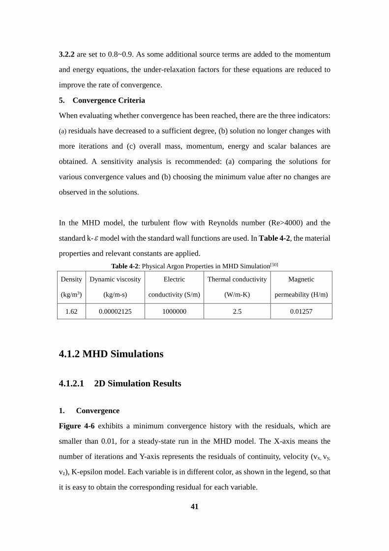
3.2.2 are set to 0.8~0.9. As some additional source terms are added to the momentum
and energy equations, the under-relaxation factors for these equations are reduced to
improve the rate of convergence.
5. Convergence Criteria
When evaluating whether convergence has been reached, there are the three indicators:
(a) residuals have decreased to a sufficient degree, (b) solution no longer changes with
more iterations and (c) overall mass, momentum, energy and scalar balances are
obtained. A sensitivity analysis is recommended: (a) comparing the solutions for
various convergence values and (b) choosing the minimum value after no changes are
observed in the solutions.
In the MHD model, the turbulent flow with Reynolds number (Re>4000) and the
standard k-ε model with the standard wall functions are used. In Table 4-2, the material
properties and relevant constants are applied. Table 4-2: Physical Argon Properties in MHD Simulation[50]
Density
(kg/m3)
Dynamic viscosity
(kg/m-s)
Electric
conductivity (S/m)
Thermal conductivity
(W/m-K)
Magnetic
permeability (H/m)
1.62 0.00002125 1000000 2.5 0.01257
4.1.2 MHD Simulations
4.1.2.1 2D Simulation Results
1. Convergence
Figure 4-6 exhibits a minimum convergence history with the residuals, which are
smaller than 0.01, for a steady-state run in the MHD model. The X-axis means the
number of iterations and Y-axis represents the residuals of continuity, velocity (vx, vy,
vz), K-epsilon model. Each variable is in different color, as shown in the legend, so that
it is easy to obtain the corresponding residual for each variable.
41

Figure 4-6: Convergence History of High-current Plasma Beam
2. Static Pressure
Energy and mass transfer processes are closely coupled in high-current plasma beams
and a static pressure distribution therefore need to be understood. Figure 4-7 shows the
static pressure distribution of outlet in the radial direction at the XY cross section, where
the X-axis denotes the radial position in plasma beam and the Y-axis denotes the static
pressure. The static pressure consists of two pressure circles, which are similar in size
and continually change. The condition for emergence of two pressure circles, which is
equivalent to the condition that the vortex current flow[51]occurs in the same way. The
phenomena is due to the non-uniformity of the argon transport coefficients in the high-
current plasma beams.
Figure 4-7: Static Pressure Distribution of Outlet in Radial Direction
42

3. Velocity Monitor
The initial velocity at the inlet is set to be vx=0, vy=0 and vz=1.2m/s. In order to monitor
the trend of velocity, the velocity monitor is put at the outlet based on mass weighted
average. Figure 4-8 shows the mass weighted average for velocity at the outlet, where
the X-axis means the number of iterations and the Y-axis means the mass weighted
average for velocity at the outlet. The outlet velocity firstly drops so fast, after 200
iterations, the mass weighted average for velocity becomes stable and close to 0.
Figure 4-8: Mass Weighted Average for Velocity at Outlet
It is useful to obtain information about the velocity magnitude distribution in the radial
direction in Figure 4-9, where the X-axis is the radial position in plasma beam and Y-
axis is the velocity magnitude. The velocity magnitude distribution is similar to a
Gaussian distribution so that we can identify that the further the distance of the central
axis, the smaller the value of the velocity magnitude. The largest velocity magnitude is
around 0.7 m/s and the smallest velocity magnitude is around 0.2 m/s. At the± 0.006m
positions, the velocity quickly drops; after that, it becomes stable.
43

Figure 4-9: Velocity Magnitude of Outlet in Radial Direction
4.1.2.2 3D Simulation Results
1. Contour
In Figure 4-10, it is concluded that the density of the high-current plasma beams is not
uniform due to non-uniform transport coefficients, and the density changes around
1.62kg/m3.
Figure 4-10: 3D Density Distribution of High-Current Plasma Beam
2. Vector
In Figure 4-11, due to the external applied magnetic fields (B0x=0.5T, B0y=0.5T,
B0z=1T), they give a helical shape of magnetic field. The Lorentz force is produced in
44

the three directions so that the velocity vector has the different magnitudes and
directions. When the velocity vector is close to the inlet, it changes to the opposite
direction at the edge of the MHD model. Near the conducting wall, the velocity vector
rotates along the Z direction. At the inner MHD model, it rotates at a higher speed than
at the edge.
Figure 4-11: 3D Velocity Vector of High-Current Plasma Beam
4.2 MC Simulation Results
The simulations of an e-beam source in the electromagnetic fields are illustrated, where
the electric fields are uniform and the magnetic fields are produced by a quadrupole. It
is critical to choose a sufficient number of iterations to score accurate results. In this
thesis, the number of initial electrons is 1,000,000, which limits the relative fluctuation
within 1%. The computations are run on the Dell INSPIRTION-PC with a 2.5 GHz
Intel core i5-2450M processor and the computation time varies from 30 minutes to five
hours.
4.2.1 Simulation Instruments
4.2.1.1 Notepad++
Notepad++ is a free source code editor as shown in Figure 4-12. Running in the 45

Windows environment, Notepad++ is written in C++ and uses the pure Win32
Application Programming Interface (API) and the Standard Template Library (STL)
which ensures a high execution speed and small program size.
Figure 4-12: Notepad++ Programming Interface
4.2.1.2 PHITS 2.64
The multi-purpose Monte Carlo Particle and Heavy Ion Transport code System
(PHITS)[52][53] based on the NMTC (Nuclear Meson Transport Code) and JAM (Jet-Aa
Microscopic Transport Model)[54] has been developed. The physical processes which
PHITS includes are divided into the two categories, as shown in Figure 4-13: transport
processes and collisions. In the transport processes, the PHITS can simulate particle
motion under external fields, such as magnetic and electric fields. Without external
fields, neutral particles move along a straight trajectory with constant energy until a
next collision. The second category is collisions. According to mean free path, the
PHITS chooses next collision point using the MC method. To generate secondary
particles of collisions, we need the information on final state of the collisions.
Figure 4-13: Particle Transport Processes and Collisions in PHITS
46

4.2.1.3 Assisted Tools
In the MC simulations, we also use assisted tools to program and display the high-
current plasma beams. In Table 4-3, the names, types and function are simply described. Table 4-3: Assisted Tools in MC Simulations
aEPS denotes the Encapsulated PostScript.
4.2.2 MC Simulation Steps
The source code of the PHITS is written in Fortran (Formula Translating System) and
the MC simulation flowchart is shown in Figure 4-14. We first specify the geometry
of 3D virtual space and the information of source particles. Next, we tally various
quantities by simulating electrons.
Figure 4-14: Flowchart of MC Simulation
1. Geometry and Material
The geometry of the high-current plasma beams is defined by the Boolean operators
including cell and surface definitions. We use infinite space and fill cells with certain
Name Type Function
ANGEL Programming
language ANGEL is used to draw fine graphs and creates EPSa files from input. It is a translator from ANGEL language to PostScript (PS) language, which interprets commands and data and creates PS files.
GSview 5.0
Graphical interface
GSview is used to display image files created by the PHITS, which are written in the EPS format.
47

materials or void: the wall (cell 101) is filled with copper, the cell 100 is filled with
argon gas and the cell 102 is void. The properties of argon gas and copper are listed in
Table 4-4. Table 4-4: Argon Gas and Copper Properties in MC Simulations
Argon Copper
Radius (cm) 2 2 (IDa)/2.5 (ODb)
Length (cm) 10 10
Density(g/cm3) 1.62e-3 8978
Initial electron projectile energy (MeV) 0.158 0
a ID denotes the inner dimension.
b OD denotes the outer dimension.
2. Source
We select a cylindrical shape of source distribution with mono-energy source particles.
The radius of the cylindrical source is 2cm and the length is 10cm. The total number of
electron source particles is 1000,000, since in the calculation of statistical uncertainties,
the history variance mode is selected, which calculate the standard deviations using
variances between tally results of each history. The standard deviation depends only on
the total history number so that relative errors are proportional to the number of history,
which is equal to the number of electron source particles. They go through the cell 100
along the Z-axis. During this process, it produces other particles, such as neutrons and
photons.
3. Tally
We use tallies [t-3dshow] and [t-gshow] to check geometries of the MC model, such as
the 2D and 3D visualizations. Besides, we use tallies [t-track], [t-heat] and [t-deposit]
to calculate physical quantities, such as particle flux, heat and deposit energy.
4. Control
Some control functions are available for us to improve the MC simulation accuracy,
such as calculation mode (icntl=0~12), particle transport simulations and physical
models. We can also obtain better statistics by increasing the history number.
48

4.2.3 MC Simulations
4.2.3.1 Geometry of MC Model
The tally [t-3dshow] gives us the 3D plasma beam geometry, as shown in Figure 4-15.
It is obvious that the argon gas is red and the copper is cyan.
Figure 4-15: 3D MC Model by Tally [t-3dshow]
In Figure 4-16, we check the 2D geometry of the MC model by the tally [t-gshow].
Since the sphere (cell 102) is hypothetical, it is assumed to be void.
(a) (b) Figure 4-16: 2D MC Model by Tally [t-gshow] on (a) XY Plane and (b) XZ Plane.
49

4.2.3.2 Amount of Particles
The tally [t-product] tallies source particles, particles and nuclei produced by nuclear
reaction and decay and its unit is [1/source]. In Figure 4-17 (a), the amount of all
particles is shown on the XZ plane and its relative errors are shown in Figure 4-17 (b).
Warm colors indicate that relative standard errors are large (close to 1), while cold
colors represent small relative standard errors. The source particles are generated in the
cell 100 and they also transport to the cell 101. In the center of the plasma beams, the
number of all particles is the most and it is equal to 10-3 [1/source] ×
1000000[source]=1000. At the edge of the plasma beams, the number of all particles
becomes small and it is smaller than 10-5 [1/source]×1000000[source]=10. From the
relative error distribution, it is obvious that it is close to 0.01.
(a)
(b) Figure 4-17: (a) Amount of Particles by Tally [t-product] and (b) The Relative Errors
In order to obtain statistical uncertainties, we calculate standard deviations using
variances between tally results of each batch and history. The standard deviation σd is
calculated by
( )( )
2 2
1/
1
N
i il
d
x w w N x
N Nσ =
−=
−
∑ (4.4)
50

where N is the total history number (istdev=2), xi and wi are the tally results and the
source weight of each sample, respectively. Therefore, x and w are the mean values of
the tally results and the source weights of N samples. The ratio of σ to x is written as
the relative error in tally output files.
4.2.3.3 Electron Flux
We check electron flux of all regions in magnetic fields by tally [t-track] and set icntl=5.
In Figure 4-18 (a) and (b), the default of the electron initial energy is from 0 MeV to
10-2 MeV. In the argon gas region (cell 100), the flux of electron is 10-3 [1/cm2/ source].
The relative errors ( 210−≈ ) are low and it is proved that the electron flux is accurate.
In the copper wall (cell 101), the electron flux is 10-4 [1/cm2/ source]. However, its
relative errors are close to 1, the electron flux is not accurate so that it should be
reasonably neglected.
51

(a)
(b) Figure 4-18: (a) Electron Flux by Tally [t-track] on XY plane and (b) The Relative Errors
Similarly, under the effect of magnetic fields (10 KG), the electron flux on the XZ plane
is shown in Figure 4-19 (a). The average electron flux is close to 10-2 [1/cm2/source]
in the argon gas region. In the cathode (left) part, the electron flux are increased from
10-6 [1/cm2/source] to 10-3 [1/cm2/source]. The electron flux in the cell 102
symmetrically distributes along the X-axis. Additionally, the inner region has the
highest value and the outward region has the lowest value. In the anode (right) part, the
electron flux is higher than that in the cathode part and its electron flux range is from
10-4 [1/cm2/source] to 10-2 [1/cm2/source]. The level line of electron flux in the anode
is not clearer than that in the cathode. In Figure 4-19 (b), the relative errors are so small
in the cells 100 and 102, so that it is convinced that the simulation results have high
accuracy. In order to finish these MC simulations, it takes 1 hour to run the [t-track]
algorithm.
52

(a)
(b) 6
Figure 4-19: (a) Electron Flux by Tally [t-track] on XZ Plane and (b) The Relative Errors
4.2.3.4 Deposit Energy Distribution
Ionization energy losses by charged particles are scored by tally [t-deposit] and its unit
is 1/source. Particles with energy below emin parameters are not traced by PHITS
simulation. We use reg mesh in the argon gas region, which is a geometrical mesh and
divides the regions in cells. The E-type=3 denotes logarithmic interval and the ANGEL
parameters (angel=ymin[1E-06] ymax[1E-00]) are used to change layouts of EPS figures.
In Figure 4-20, the deposit energy distribution has Gaussian distribution. From the 10-
2 to 10-1 MeV, the particles are the most. Since the total number of particles is 1,000,000,
more than 10,000 source particles have 10-2~10-1MeV energy. With the increases of the
53

deposit energy from being 10-7 MeV, the number of particles are growing.
Figure 4-20: Deposit Energy by Tally [t-deposit] in Cell 100
4.2.3.5 Heat Distribution
During the processes of argon gas excitation and ionization, neutrons and photons are
produced. We can use tally [t-heat] to calculate neutrons and photons dose by the
Kinetic Energy Released per unit Mass (KERMA) approximation. In the thesis, for
electron=1 with electron transport, we do not use the KERMA factors of photon, but
obtain the heat from the energy loss of electrons. In Figure 4-21(a), the heat in the
cathode region is lower than that in the anode region and the value is smaller than 10-6
[MeV/source]. The heat is almost uniform except the cathode part. There are still some
heat in the cell 101 due to neutrons penetrating into the copper wall. However, the heat
is smaller than 10-8 [MeV/source]. In Figure 4-21(b), the relative errors of heat are
smaller than 0.1 in the cell 100. The relative errors at the edge of copper is not
reasonable, which can be optionally neglected. It takes around 1 hour 16 minutes to
obtain the heat distribution and its relative errors.
54

(a)
(b) Figure 4-21: (a) Dose of Neutrons and Photons by Tally [t-heat] and (b) The Relative Errors
4.3 IMHDMC Simulation Results
The IMHDMC method is a comprehensive method that integrates the MHD and MC
simulation results together. It links the magnetohydrodynamic fluid with the particle
transports and collisions in the high-current plasma beams. The MHD simulations
define spatial distribution of electric fields and these distribution are then employed by
the MC simulations to characterize heat and deposit energy. The Ar0 are assumed to
have a uniform density (1.65×1016 cm-3) at the simulation conditions.
55

(a)
(b)
Figure 4-22: 1D Density Profiles of (a) e- and (b) Ar+ in IMHDMC Model
Figure 4-23: Validation of IMHDMC Method by References
In Figure 4-22(a) and (b), the electron density is almost same as the Ar+ density in the
high-current plasma beams, where the horizontal axis is the X-axis and the Y-axis is
the electron density. In Figure 4-23, the line 1 denotes the fluid model, the line 2
denotes the extended fluid model, the line 3 denotes the hybrid model, which is
equivalent to the IMHDMC model in the thesis; and the point line denotes the
reference[55] data. The vertical lines in Figure 4-23, represent the borders between the
0
0.8
1.41.6
1.9 1.9 1.91.7
1.30.9
0.10
0.5
1
1.5
2
-5 -4 -3 -2 -1 0 1 2 3 4 5Dens
ity (1
0^11
cm
^-3)
X(cm)
e-
0.2
0.7
1.21.6
1.8 1.9 1.91.7
1.3
0.8
0.30
0.5
1
1.5
2
-5 -4 -3 -2 -1 0 1 2 3 4 5
Dens
ity ()
10^1
1 cm
^-3)
X(cm)
Ar+
56

cathode sheath and negative glow regions of the discharge for the different models.
Compared to the results, which are the electron and ion densities, in Figure 4-23, the
simulation results in Figure 4-22 computed by the IMHDMC model lead to the closer
plasma densities.
In Figure 4-24(a), the temperature distribution produced by the IMHDMC method
correspond to the MHD and MC simulation results. The ANSYS FLUENT MHD
module is used for the MHD simulations, while the PHITS is used for the MC
simulations. According to the IMHDMC simulation results in Figure 4-24(b), the
Lorentz force is the main parameter which affects the fluid flow in the magnetic fields.
In the center of the high-current plasma beams, there is the largest Lorentz force.
(a) (b)
Figure 4-24: (a) Temperature Distribution and (b) The Lorentz force in IMHDMC Model
4.4 Experimental Verification
The main purpose of the HOPE’s experiment is to test the formation of a high-current
plasma beam, which will be used to guide the construction of an apparatus. The same
four plasma beams are arranged into a balanced tetrahedral structure so that all four
beams will pass through a central focal point.
4.4.1 Current-Voltage Relation
Current I(t) in an electric circuit is defined as the rate of flow of a charge Q(t) passing
through it. Thus the charge on the electrodes is equal to the integral of the current as
57

well as proportional to the voltage. It is assumed that the initial voltage is equal to zero
and there is no resistance through a plasma or wires. This is the integral form of
capacitor equation[56]:
( )0
( ) 1( )t
t
Q tV t I t dtC C
= = ∫ (4.5)
where V is the voltage across the capacitor, Q is the charge stored in the capacitor, C is
the capacitance and I is the current.
Taking derivative of Equation 4.5 and multiplying by C produces the derivative form: ( ) ( )( ) dQ t dV tI t C
dt dt= = (4.6)
After obtaining the relationship between a voltage and time, it is easy to calculate a
current produced by a DC discharge.
4.4.2 High-Current Plasma Beam Experiment
In Figure 4-25, the test setup with capacitors is set at the near-vacuum ambient pressure
to produce a DC discharge. The capacitors then discharge an electric current between
the electrodes, with transient electromagnetic fields accelerating the resulting plasma.
This test setup basically consists of a cylindrical quartz chamber, necked at both ends
to accommodate stainless steel end flanges and seals. The electrodes and some
instrumentation ports pass through the end flanges. Not shown in the figure is the
fueling flow loop and small tank. A vacuum pump can be connected to the fitting on
the flange in the foreground. The initial conditions are as follows in Table 4-5.
58

Figure 4-25: HOPE’s Test Setup[57]
Table 4-5: Initial Conditions under Steady State in HOPE’s Experiment
Parameter Value
Atmosphere temperature 300K
Inlet pressure 110kPa
Ambient pressure 10-3Pa
Voltage 150V
Constant capacitance 1.00054 Fµ
Figure 4-26: High-current Plasma Beams Formed across Two Plasma Jets[58]
To initiate a plasma, a voltage is applied to both ends of the single carbon tube passing
59

through the chamber. A notch or a length of thinner tube is made at the center point of
the carbon tube. The tube vaporizes starting from the center thinned-down location, and
a high-current plasm beam is generated and maintained by the supplied voltage and
current, as shown in Figure 4-26. When the current passing through the argon gas is
high enough, a pinched plasma beam forms under the influence of the Lorentz force.
The remaining halves of the tubes continue to act as the electrodes to feed current
through plasma beams. The high temperature plasma as well as the current continue to
vaporize the ends of the carbon graphite tube and widen the gap until the tube is
consumed or until its temperature no longer increases. The plasma beam is extinguished
when the gap between the electrodes exceeds the length at which the voltage are needed
to maintain high-current plasma beams.
4.4.3 Experimental Results and Analysis
1. Power Supply
1) Rippled DC, rectified from 60Hz AC supply with 12 pulses per cycle
2) Max 640V adjustable (± 320V with center tap connected to ground potential)
3) Max 8kA adjustable
4) Operation mode: current mode
2. Gas Supply
Argon is initially used to fill the test chamber and subsequently fed into the carbon
graphite tube from the negative terminal.
4.4.3.1 Measurement
The voltage, current and temperature are measured in HOPE’s experiment as following:
1) Voltage should be measured directly between the two electrodes;
2) Current is measured using the inductance pickups near the apparatus;
3) Thermocouples are placed on the electrodes, quartz chamber and cooling blocks
and on any temperature-sensitive components;
60

4) Methods for measuring plasma temperature and cation and electron speed in the
plasma are being developed in collaboration with HOPE’s R&D partners.
4.4.3.2 Experimental Data
In Figure 4-27(a), we can see that the voltage and current continuously change with
the time. The two solid lines denote the polynomial fittings of the voltage and current.
The average of voltage and current are approximately 150 V and 335A. In Figure 4-
27(b), we can obtain the relationship between the voltage and current and directly read
their polynomial equations.
(a)
(b)
Figure 4-27: (a) Current (Red Line) & Voltage (Blue Line) vs. Time and (b) Polynomial Equation for Voltage vs. Current in HOPE’s Experiment
In Figure 4-28, in the beginning, the temperature violently changes. With the time goes
by, it changes more steadily. During the process, although the power increases, the
-300
-100
100
300
500
700
900
0100200300400500600700800900
1000
168.
317
3.9
179.
518
5.1
190.
719
6.3
201.
920
7.5
213.
121
8.7
224.
322
9.9
235.
524
1.1
246.
725
2.3
257.
926
3.5
Current (A)
Voltage (V)
Time (s)
y = 0.0005x3 - 0.1981x2 + 19.332x - 32.965
-200
0
200
400
600
800
1000
-10 40 90 140 190 240
Current(A)
Voltage (V)
61

temperature does not change irregularly, which is approximately equal to 1500K.
Figure 4-28: Power vs. Temperature in HOPE’s Experiment
4.4.3.3 One-Way Analysis of Variance
From the summary part in Table 4-6 and Table 4-7, we obtain the sum, mean and
variance of voltage and current, respectively. From the ANOVA part, in Table 4-6,
because p is equal to 0.667554, which is larger than 0.05 at the 0.05 level, the mean
difference is not significant. Similarly, in Table 4-7, because P-value is equal to
0.078316, which is larger than 0.05 at the 0.05 level, the mean difference is not
significant. Therefore, the changing time has no significant influence on the voltage
and current measurement. This means that the measured values are close to the
calculated theoretical values.
We also see that the variance sources come from three parts: variance between groups,
variance within groups and variance in total groups.
0250500750
100012501500175020002250250027503000
0 50 100 150 200 250 300 350 400 450 500 550 600 650 700 750 800 850
Tem
pera
ture
(K)
Power (W)
62

Table 4-6: Analysis of Variance (ANOVA) Table for Voltage
Summary
Groups of current Number Sum Mean Variance
Group 1 12 1821 151.75 7.295455
Group 2 12 1816 151.3333 3.69697
ANOVA
Difference source SS Df MS F-ratio P-value
Between groups 1.041667 1 1.041667 0.189524 0.667554
Within groups 120.9167 22 5.496212
Total 121.9583 23
Table 4-7: ANOVA Table for Current
Summary
Groups of current Number Sum Mean Variance
Group 1 12 3945 328.75 381.8409
Group 2 12 4157 346.4167 716.6288
ANOVA
Difference source SS Df MS F-ratio P-value
Between groups 1872.667 1 1872.667 3.409592 0.078316
Within groups 12083.17 22 549.2348
Total 13955.83 23
where SS denotes sum of squares, Df denotes degree of freedom and MS denotes mean square.
4.4.4 Three Methods Verification
1. Quantitative Plasma Energy
For plasma energy in the MHD simulations using Equation 3.3 in Section 3.2.2, the
energy of a plasma equals to the sum of thermal energy, Ohm’s heating and radiation.
The energy density, Ed, is the summation of the internal energy, the kinetic energy and
the energy of the magnetic field[59] with the unit J:
63

0
1 .1 2 2d
h
p B BE v vr
ρµ⋅
= + +−
(4.7)
where the term02
B Bµ⋅
denotes the plasma energy of magnetic field, which are assumed to
be produced from either plasma by an external magnetic field.
For plasma energy in the MC simulations, the electron flux and deposit energy are used
to calculate the plasma energy with the unit 109eV. For plasma energy in the HOPE’s
experiment, power is equivalent to the plasma energy with the unit W. For the IMHDMC
method, it combines the MHD and MC simulations so that the sum of them represent
plasma energy in the IMHDMC simulations. In Figure 4-29, the MHD, MC and
HOPE’s experiment plasma energy are illustrated, where the X-axis is the length of the
plasma beam and the Y-axis is the plasma energy. It is obvious that each of plasma
energy increases along the Z-axis over time and the plasma energy from the three
simulation methods are consistent with the plasma energy from the HOPE’s experiment.
Figure 4-29: HOPE’s Experiment (blue line), MHD Simulation (red line) and MC Simulation
(black line) for Plasma Energy
2. Qualitative Plasma Dynamics
In the MHD simulation results, the static pressure (p=κ nT) is not stable and this
phenomenon corresponds to the changing temperature in the HOPE’s experiment. In the
MC simulation results, the amount of particles and heat are the most in the center of the
plasma beam. It corresponds to the lightest portion in the center of the plasma beam in
0
20
40
60
80
100
120
140
160
0
1000
2000
3000
4000
5000
6000
7000
1 2 3 4 5 6 7 8 9 10
Plas
ma
Ener
gy
Plas
ma
Ener
gy
Length (cm)
64

the experiment. In the IMHDMC simulation results, the temperature is the highest in the
center of the plasma beam. It corresponds to the highest temperature with the similar
value in the experiment. Therefore, the plasma dynamics from the three method
simulations have good similarities with the experimental data. To some degree, the three
methods are verified in this aspect.
Finally, it is concluded that the three method simulation results are quantitatively and
qualitatively consistent with the experimental data.
65

5 Chapter 5: Comparison, Analysis and
Discussion
In Chapter 5, we evaluate the MHD, MC and IMHDMC methods. Firstly, in Section
5.1, the comparisons between the MHD and MC methods are presented according to
the simulation results. In Section 5.2, the discussion shows that the three new methods
have their own special features and advantages.
5.1 Comparison and Analysis
High-current plasma beams are modeled by the ANSYS FLUENT MHD module. The
theory of the MHD module, along with the governing equations in the differential form
and boundary conditions, are given. According to the MHD simulation results, the
Lorentz force is a main parameter which affects a fluid flow in magnetic fields. In the
MC method, the high-current plasma beams are simplified as beams ionized by the e-
beam source in the magnetic fields. The MC method includes the particle transport
process and collision. According to the MC simulation results, the magnetic fields in
the PHITS geometries change the particle trajectories. The heat and deposit energy are
increased by the magnetic fields. The similarities and differences between the MHD
and MC simulations are listed in Table 5-1.
66

Table 5-1: Similarities and Differences between MHD and MC Simulations Similarities 1) Same geometry: two cylinders
2) Same materials: argon gas and a copper wall 3) Same parameter values: length and radius
Differences
1) Different states: the steady state for the MHD method and the transient state for the MC method
2) Different initial settings: the initial velocity for the MHD method and the initial projectile energy of electron for the MC method
3) Different evaluation standards: tolerance for the MHD method and relative errors for the MC method
4) Different running time: 10-20minutes per simulation for the MHD method and 30-100 minutes per simulation for the MC method
5) Different control functions: solution control panel for the MHD method; history number, cut-off energy and data libraries function for the MC method
5.2 Discussion
5.2.1 Theoretical Aspect
The MHD, MC and IMHDMC methods are compared in Table 5-2. These three new
methods are all used to study plasma dynamics. However, none of them is capable of
simulating plasma transition from a collisionless regime to collisional regime[60]. Only
the MC method can be used to study electron motion. The MHD method assumes quasi-
neutrality and neglects mass of electrons. The IMHDMC method is a comprehensive
frontier, which bridges collisional and collisionless transition. Table 5-2: Comparison between MHD, MC and IMHDMC Methods
MHD method MC method IMHDMC method Approach Continuum Particles Continuum & Particles Advantage Accurate Easy for complex problems
and easy for coding Easy for coding and the
fastest one Disadvantage Numerically
instability Crude (with error∝ 1/ N )) Too many chemical
reactions and particles considered
67

5.2.2 Simulation Aspect
Firstly, in the MHD simulation results, we obtain the static pressure radial distribution
and the radial velocity magnitude at the outlet. We also simulate the 3D velocity vector
by the vector function. In the MC simulation results, we use the tallies to describe the
electron flux on the XY and XZ planes, and the heat and deposit energy distribution.
Finally, using the IMHDMC method, which links the MHD and MC simulations
together, we can accomplish more accurate and reasonable simulation results: (a) the
density profiles calculated by the MC method and (b) the temperature and Lorentz force
distribution calculated by the MHD method.
Secondly, the computation time is important and can be regarded as one of simulation
difficulties. The MC method approximately takes five hours, the MHD method takes
less than one hour and the IMHDMC method takes three hours. The simulation
difficulties can be intentionally adjusted by reducing the mesh quality. Therefore, the
computational resource is a critical component for MHD, MC and IMHDMC
simulations, especially for the MC simulations. The computer resources will be
required for more accurate and extensive simulations.
Thirdly, the models of high-current plasma beams in this thesis are not perfect.
Although the MHD, MC and IMHDMC simulations are very useful, some details in the
simulations are neglected and assumed. For example: in the MHD simulations, the
high-current plasma beams are assumed to be turbulent fluid; in the MC simulations,
the electric fields are assumed to be uniform; and in the IMHDMC simulations,
metastable argon is neglected. There are several other models that could be used to
simulate high-current plasma beams, such as the two-fluid model. Therefore, further
corrections would be necessary for more accurate simulations.
68

6 Chapter 6: Conclusion and Future Work
6.1 Conclusion
Using the MHD, MC and IMHDMC methods, we have reached the state in which the
3D simulations with detailed geometry descriptions for high-current plasma beams are
conducted. The MHD, MC, and IMHDMC simulations have helped us achieve a better
understanding of dynamics of high-current plasma beams. For example: in industrial
applications, the simulations could help us improve plasma torch design and fusion
energy generation controlling. However, some improvements could be achieved with a
higher computing power and the massive use of parallel computing. Most importantly,
the complexity of models that are capable of simultaneously describing different
processes, has been a limiting factor for high-current plasma beam simulations.
After we identify the velocity and pressure changes by the MHD method; the electron
flux and deposit energy by the MC method; and the density, temperature and Lorentz
force distribution by the IMHDMC method, it is so important to provide the ability to
implement plasma control applications, such as fusion energy generation cooling. It
should be pointed out that the high-current plasma beam simulations performed by the
MHD, MC and IMHDMC methods in this thesis display a useful starting point to study
more complex problems, such as unsteady MHD flow.
6.2 Potential Applications
6.2.1 Fusion Energy Generation Application
The HOPE’s Z-Pinch Experiment is an innovative confinement concept to magnetically
confine a high-temperature and high-density plasma. A Z-pinch has a simple and linear
configuration with no magnetic field coils: axial plasma current generates azimuthal
magnetic fields that confine and compress the plasma. The Z-pinch concept is
69

investigated in formative years of fusion energy development. Plasma instabilities, such
as sausage and kink modes, limit achievable parameters and hinder progress of the Z-
pinch concept. However, more recent theoretical investigations have presented a
mechanism to stabilize Z-pinch plasmas using a shear flow. In Figure 6-1, there is a
basic explanation of how a Z-pinch works.
1. Pinches apply a huge voltage across a tube, which is filled with fusion fuel. The gas
ionizes when the voltage times charge is higher than ionization energy of a gas.
2. Current jumps across this gap.
3. The current makes magnetic fields which are perpendicular to the current. This
magnetic fields try to pull material together.
4. These atoms could draw close enough to fuse.
Figure 6-1: Basic Z-pinch Mechanism[61]
The HOPE has developed an alternative approach to generate fusion energy based on
the concept of four high-current plasma beams passing through a common intersection
point called the focal region[62], as shown in Figure 6-2. The four high-current plasma
beams are symmetrically arranged in 3D space in a tetrahedral configuration. This
innovative configuration can improve plasma stability in the focal region.
Figure 6-2: Four Intersecting Plasma Beam Model[63]
70

6.2.2 Plasma Gasification Application
Plasma gasification is a process which converts organic matter into synthetic gases,
electricity and slag by using high-current plasma beams. In Figure 6-3, the two plasma
arc torches are the main elements and are powered by electric arcs. The plasma
gasification is commercially used as a form of waste treatment. A plasma torch uses
an inert gas and electrodes vary from copper to tungsten and other alloys. High current
are produced by high voltage, which pass between two electrodes to produce a high-
current plasma beam (an electric arc). The pressurized inert gas is ionized passing
through the plasma beam. When the torch temperature is very high, molecular bonds
break down to create basic material atoms.
Figure 6-3: Westinghouse Plasma Gasification. (Westinghouse Plasma Corporation)[64].
Waste processing by plasma gasification is an ecologic process, as shown in Figure 6-
4. Due to lack of oxygen and existing high temperature in a waste processing reactor,
it prevents main elements of gases from forming toxic compounds, such as NOx. The
filtration systems remove inorganic residue and gaseous pollutants so that they produce
clean synthetic gases. At the same time, the circulating water in the filtering systems
has removed hazardous substances. Next, the synthetic gases produced by the last step
is used for power supply and the gaseous pollutants are converted to valuable chemical
71

products. Finally, the inert slag is used in construction and the left metal is used for
production of alloy.
Figure 6-4: Waste Processing by Plasma Gasification
6.3 Future Work
Optimization of the MHD, MC and IMHDMC models of high-current plasma beams in
industrial applications, may improve their performance further. A list of prospective
optimizing activities may include:
1. The mesh grid quality in the three models could be improved by using a different
type of mesh grids since mesh grids are varied in geometry, boundary conditions
and material. The improvements could be conducted by iteratively changing size
and shape of elements and relative dimensions of neighboring elements.
2. Other pure gases or mixtures could be applied in the three models. After we have
a wide range of simulation results, it is easy to choose the most efficient gases or
mixtures in industrial applications.
72

In the future, we will do other useful measurement and development for HOPE’s
experiment. For example, we could use a Langmuir electrostatic probe to measure
electron density and temperature. At the same time, because the magnetic fields in the
plasma are periodic, the rate of change of the magnetic field with time can be measured
locally by magnetic probe. More intersecting plasma beams would be applied to the
MHD, MC and IMHDMC models. The interaction effects can be explored between the
two or more plasma beams using the MHD, MC and IMHDMC methods. Besides,
prospective activities would involve a separate validation for the IMHDMC method.
73

Appendices
Appendix A: List of Acronyms
1D/2D/3D One/ Two/ Three Dimensional
API Application Programming Interface
ANOVA Analysis of Variance
CFD Computational Fluid Dynamics
DC Direct current
Df Degree of freedom
e-beam electron beam
EPS Encapsulated PostScript
FEM Finite Element Method
Fortran Formula Translating System
FVM Finite Volume Method
GG General Geometry
HOPE HOPE Innovations Inc.
ID Inner Dimension
IMHDMC Integrated Hybrid MHD and MC Method
k-ε K-epsilon
KERMA Kinetic Energy Released per unit Mass
LTE Local Thermodynamic Equilibrium
MCNP Monte Carlo N-Particle
MHD Magnetohydrodynamics
MS Mean square
NEC Net Emission Coefficient
NMTC Nuclear Meson Transport Code
OD Outer Dimension
PDEs Partial Differential transport Equations
74

PENELOPE Penetration and ENErgy Loss of Positrons and Electrons
PHITS Particle and Heavy Ion Transport code System
PIC Particle-In-Cell
PS PostScript
PTSG Plasma Theory and Simulation Group
RDD Radiological Dispersal Device
SIMPLE Semi-Implicit Method for Pressure-Linked
SS Sum of squares
STL Standard Template Library
Appendix B: Nomenclature
Ar0 argon atoms
Ar+ argon ions
B magnetic field
cs speed of sound in a plasma
C capacitance
Cp specific heat
d distance
e electron charge
e- electron
Ec cut-off energy
Ed plasma energy density
Ek kinetic energy
F Lorentz force
h specific total enthalpy
I current
J current density
Kn Knudsen number
L number of steps
75
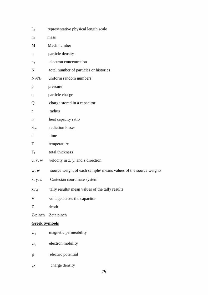
Lr representative physical length scale
m mass
M Mach number
n particle density
ne electron concentration
N total number of particles or histories
N1/N2 uniform random numbers
p pressure
q particle charge
Q charge stored in a capacitor
r radius
rh heat capacity ratio
Srad radiation losses
t time
T temperature
Tt total thickness
u, v, w velocity in x, y, and z direction
wi/ w source weight of each sample/ means values of the source weights
x, y, z Cartesian coordinate system
xi/ x tally results/ mean values of the tally results
V voltage across the capacitor
Z depth
Z-pinch Zeta pinch
Greek Symbols
0µ magnetic permeability
eµ electron mobility
φ electric potential
ρ charge density 76

κ Boltzmann constant
0ε electric permittivity
ξ energy
τ viscous stress
η electrical resistivity
λ thermal conductivity
mλ mean free path
σ electrical conductivity
σd standard deviation
θ /ϕ polar angle
ω cyclotron frequency
Subscripts
e electron
exc excitation
EAS EquiAngle Skew
i ion
ion ionization
max maximum
min minimum
p particle
Appendix C: Physical Constants
Permittivity of free space 120 8.8542 10 /F mε −= ×
Permeability of free space 70 4 10 /H mµ π −= ×
Boltzmann constant 231.3807 10 /J Kκ −= ×
Standard pressure (760Torr=1atm) P0=1.0133×10⁵ Pa
Absolute zero temperature T0= 273.15 C− ° 77

Elementary charge q=-1.602×10⁻¹⁹C
In plasma physics, we often uses electron volts (eV) and 1eV≈1.1604×10⁴K. In SI
units we use Tesla (T) and Gauss (G) for magnetic flux densities amd1G=10-4T.
78

References
[1]Anthony L. Peratt, “Advances in Numerical Modeling of Astrophysical and Space
Plasmas”, Astrophysics and Space Science, Vol 242 (1-2), pp: 93-163, 1997. [2]B. R. Adhikari, R. Khanal, “Introduction to The Plasma State of Matter”, The
Himalayan Physics, Vol 4 (4), pp:60-64, 2013.
[3]Francis F. Chen, “Introduction to Plasma Physics and Controlled Fusion (Volume 1:
Plasma Physics) (Second edition)”, Plenum Press, New York and London, 1929.
[4]Daniel J. Ellard, Penelope A. Ellard, “The Monte Carlo Method” in S-Q 1998 Course
Book, pp: 106-113, 1998.
[5 ]T. Sato, K. Niita, N. Matsuda, S. Hashimoto, et al., “Particle and Heavy Ion
Transport Code System PHITS, Version 2.52”, Journal of Nuclear Science and
Technology, Vol 50 (9), pp: 913-923, 2013.
[6]Michael P. Marder, “Condensed Matter Physics”, John Wiley & Sons, Inc., Second
edition, 2010. [7]Sudeep Bhattacharjee, “Introduction: Theoretical Approach” in Compact Plasma
Focused Ion Beams, US: Taylor & Francis Group and The CRC Press, 2013.
[8]Lu B, Xu L, Zhang X, “Three-dimensional MHD simulations of the electromagnetic
flowmeter for laminar and turbulent flows”, Flow Measurement and Instrumentation,
Vol 33, pp: 239–243, 2013. [9]A Lebouvier, S A Iwarere, D Ramjugernath, et al., “3D Magnetohyrdrodynamic
Modelling of A Low-Current Plasma Arc Batch Reactor at Very High Pressure in
Helium”, Journal of Physics D: Applied Physics, Vol 46 (145203), 2013.
[10]Bycan Ibrahimoglu, Ahmet Cucen, M. Zeki Yilmazoglu, “Numerical Modelling of
DC Arc Plasma Torch with MHD Module”, International Plasma Technologies
Congress, 2014.
[ 11 ]ANSYS FLUENT Magnetohydrodynamics Module Manual, ANSYS
Incorporation, 2013.
[12] WIKIPEDIA The Free Encyclopedia. (2015, June. 1). K-epsilon turbulence model.
[Online]. Available: https://en.wikipedia.org/wiki/K-epsilon_turbulence_model
79

[13]G. Xu, Junling Hu, H. L. Tsai, “Three-dimensional Modelling of The Plasma Arc
in Arc Welding”, Journal of Applied Physics, Vol 104 (103301), 2008.
[ 14 ]E. G. Sheikin, “Monte Carlo Simulation of Non-equilibrium Conductivity
Produced by Electron Beam in MHD Flows”, 48th AIAA Aerospace Sciences Meeting
Including the New Horizons Forum and Aerospace Exposition January 2010, Oriando,
Florida
[15]Ondrej Sila, Pavel Kubes, Josef Kravarik, et al., “Estimation of amount of scattered
neutron at Devices PFZ and GIT-12 by MCNP Simulations”, Acta Polytechnica, Vol 53
(2), pp:228-232, 2013.
[ 16 ]Fawaz Ali, “On The Integration of Computational Fluid Dynamics (CFD)
Simulations with Monte Carlo (MC) Radiation Transport Analysis”, Master Thesis:
University of Ontario Institute of Technology, 2009.
[ 17 ]Qing Yang, “A Computational Fluid Dynamic Approach and Monte Carlo
Simulation of Phantom Mixing Techniques for Quality Control Testing of Gamma
Cameras”, Master Thesis: University of Canterbury, 2013.
[ 18 ]Impedans Limited Company. (2015, Sept. 25). Langmuir Probe. [Online].
Available: http://www.impedans.com/langmuir-probe
[19]WIKIPEDIA The Free Encyclopedia. (2015, June. 16). Knudsen Number. [Online].
Available: https://en.wikipedia.org/wiki/Knudsen_number
[20]Annemie Bogaerts, Renaat Gijbels, “Hybrid Monte Carlo-fluid modeling network
for an argon/ hydrogen direct current glow discharge”, Spectrochimica Acta Part B, Vol
57, pp: 1071-1099, 2002.
[ 21 ]Alexandre lebouvier, Clarisse Delanlondrer, Francois Fresnet, et al., “Three-
Dimensional Unsteady MHD Modeling of A Low-Current High-Voltage
Nontransferred DC Plasma Torch Operating with Air”, IEEE Transactions on Plasma
Science, Vol 30 (9), 2011.
[22]He-Ping Li, E. Pfender, “Three Dimensional Modeling of The Plasma Spray
Process”, Journal of Thermal Spray Technology, Vol 16 (2), 2007. [ 23 ]WIKIPEDIA The Free Encyclopedia. (2015, January. 16). Magnetic Reynolds
Number. [Online]. Available: https://en.wikipedia.org/wiki/Magnetic_Reynolds_number
[24]K. C. Hsu, K. Etemadi, E. Pfender, “Study of The Free-Burning High-Intensity
Argon Arc”, Journal of Applied Physics, Vol 54 (3), pp:1293-1301, 1993.
[25] E. Gedik, H. Kurt, Z. Recebli, “CFD Simulation of Magnetohydrodynamic Flow 80

of A Liquid-Mental Galinstan Fluid in Circular Pipes”, Technology Science Press, Vol
19(1), pp:23-33, 2013. [26]D’Angola A, Colonna G, Gorse C and Capitelli M, “Thermodynamic and transport
properties in equilibrium air plasmas in a wide pressure and temperature range”, The
European Physical Journal D, Vol 46, pp: 129–150, 2008.
[27]Naghizadeh-Kashani Y, Cressault Y and Gleizes A, “Net emission coefficient of air
thermal plasmas”, Journal of Physics D: Applied Physics, Vol 35, pp: 2925–2934, 2002.
[28]A. B. Murphy and C. J. Arundell, “Transport coefficients of argon, nitrogen,
oxygen, argon nitrogen and argon-oxygen plasmas”, Plasma Chemistry and Plasma
Processing, Vol 14, pp: 451- 490, 1994.
[29]J. P. Trelles, C. Chazelas, A. Vardelle, et al., “Arc Plasma Torch Modelling”,
Cornell University Library. [Online]. Available:
http://arxiv.org/ftp/arxiv/papers/1301/1301.0650.pdf
[30]White WB, Johnson SM and Dantzig GB, “Chemical Equilibrium in Complex
Mixtures”, Santa Monica, CA: RAND Corporation, 1957.
[31]Menart J, Heberlein J and Pfender E, “Line-by-line method of calculating emission
ceofficients for thermal plasmas consisting of monatomic species”, Journal of
Quantitative Spectroscopy and Radiative Transfer, Vol 56, pp: 377–98, 1996.
[32]Evans D L and Tankin R S, “Measurement of emission and absorption of radiation
by an argon plasma”, Physics of Fluids, Vol 10, pp: 1137–1144,1967.
[33]S.G Jennings, “The Mean Free Path in Air”, Journal of Aerosol Science, Vol 19 (2),
pp: 159-166, 1988.
[34]Ryuichi Shimizu and Ding Ze-Jun, “Monte Carlo modelling of electron-solid
interactions”, Progress Physics, pp:487-531, 1992
[ 35 ]Multi-Purpose Particle and Heavy Ion transport code System, “PHITS Basic
Lecture II: Definitions of Tally”, 2015.
[ 36 ]Katsuhisa Koura, “Null-Collision Technique in The Direct-Simulation Monte
Carlo Method”, Physics of Fluids, Vol 29 (11), pp: 3509-3511, 1986.
[37]H. R. Skullerud, “The stochastic computer simulation of ion motion in a gas
subjected to a constant electric field”, Journal of Physics D: Applied Physics, Vol 1(11):
1597, 1968.
81

[38]R. Razdan, C. E. Capjack, and H. J. J. Seguin, “Influence of a magnetic field on the
growth of instabilities in a helium glow discharge using Monte Carlo simulation of the
cathode fall region”, Journal of Applied Physics, Vol 57: 4954, 1985.
[39]R. Razdan, C. E. Capjack, and H. J. J. Seguin, “Monte Carlo simulation of the
cathode fall region of a CO2 laser glow discharge for studying the influence of magnetic
fields on instability growth”, Applied Optics, Vol 25 (17), pp: 2915-2925, 1986. [40]Hossam A. Gabber, Luping Zhang, Emmanuel Boafo et al., “3D Time-Dependent
Simulation of High-Current Plasma Beam Model by Magnetohydrodynamics and
Monte Carlo Methods”, Plasma Science Technology, Paper submitted, 2015.
[41]Jun Li, Qing-Ming Chen, Zai-Guang Li, “Monte Carlo Simulation of Electron
Motion in The Cathode Region of A Magnetron Glow Discharge in Argon”, Journal
of Physics D: Applied Physics, Vol 28, pp:681-688, 1994.
[42]Dai Sheng Mao and Qing Ming Chen, “Monte Carlo simulation of electron motion
in magnetically confined CO gas laser discharges”, Journal of Physics D: Applied
Physics, Vol 28, pp:1111-1120, 1995.
[ 43 ]A.V. Phelps. (2015, Sept. 25). PHELPS database. [Online]. Available:
http://fr.lxcat.net/data/set_type.php
[44]Annemie Bogaerts, Erik Neyts, Renaat Gijbels, et al., “Gas Discharge Plasmas and
Their Applications”, Specrochimica Acta Part B, Vol 57, pp: 609-658, 2002.
[ 45 ]Annemie Bogaerts, “Hybrid Monte Carlo-Fluid Modelling Network for An
Argon/Hydrogen Direct Current Glow Discharge”, Spectrochimica Acta Part B, Vol 57,
pp: 1071-1099, 2002.
[46] ANSYS FLUENT 12.0 User’s Guide. (2009). ANSYS Incorporation. [Online].
Available: http://users.ugent.be/~mvbelleg/flug-12-0.pdf
[47]WIKIPEDIA The Free Encyclopedia. (2015, August. 21). Mach number. [Online].
Available: https://en.wikipedia.org/wiki/Mach_number
[48]Masoud Yousef Ramandi, “Muti-Dimensional Modeling of Transient Transport
Phenomena in Molten Carbonate Fuel Cells”, PHD Dissertation, University of Ontario
Institute of Technology, 2012.
[49]ANSYS Inc., “Pressure-based Solver” in FLUENT 6.3 Documentation. [Online].
Available: https://www.sharcnet.ca/Software/Fluent6/html/ug/node987.htm
82

[50]Bo Lu, Liangwang Xu, Xiaozhang Zhang, “Three-Dimensional MHD Simulations
of The Electromagnetic Flowmeter for Laminar and Turbulent Flows”, Flow
Measurement and Instrumentation, Vol 33, pp: 239-243, 2013.
[51]E. Eylenceoglu, I. Rafatov, and A. A. Kudryavtsev, “Two-dimensional hybrid
Monte Carlo-fluid modelling of dc glow discharges: Comparison with fluid models,
reliability, and accuracy ”, Physics of Plasmas, Vol 22: 013509, 2015.
[52]H. Iwase, K. Niita, T. Nakamura, “ Development of general-purpose particle and
heavy ion transport Monte Carlo code ”, Journal Nuclear Science and Technology, Vol
39 (1142), 2002.
[53]K. Niita, T. Sato, H. Iwase, H. Nose, H. Nakashima, L. Sihver, “ PHITS-a particle
and heavy ion transport code system ”, Radiation Measurements, Vol 41 (1080), 2006.
[54]K. Niita, et al. “High Energy Particle Transport Code NMTC/JAM”, JAERI-
Data/Code 2001-007, Japan Atomic Energy Research Institute, 2001. [55]A Derzsi, P Hartmann, I Korolov, et al., “On The Accuracy and Limitations of Fluid
Models of The Cathode Region of DC Glow Discharge”, Journal of Physics D: Applied
Physics, Vol 42 (22), 2009.
[ 56 ]WIKIPEDIA The Free Encyclopedia, Capacitance, (2015, Sept.5). [Online].
Available: https://en.wikipedia.org/wiki/Capacitance
[ 57 ]W. Liu, A. Wallace, “Single Plasma Beam Experiment Test Plan”, HOPE
Document No. SL14-01-WP-001-R00-CONF from HOPE Innovations Inc., 2014.
[58]B. O. Deng, Z. X. Gan, J. J. Gu, et al., “Fusion Power Based on A Symmetrical
Plasma Beam Configuration”, A scientific paper to be submitted for publication, 2014. [59]Clyde Albert Jr. Barry Stoute, “Hybrid Electric Thruster Using Gas Mixtures”,
PHD Dissertation, York University, 2013.
[60]S. A. Ledvina, Y. J. Ma et al., “Modeling and Simulating Flowing Plasmas and
Related Phenomena”, Space Science, 2008.
[ 61 ]Wikipedia, the free encyclopedia. (2015, Sept. 10). Pinch (Plasma Physics).
[Online]. Available: https://en.wikipedia.org/wiki/Pinch_(plasma_physics)
[62]F. Miao, X. J. Zheng, and B. Q. Deng, “Fusion of Multi-pinched Plasma Beam
Converging with Spatial Symmetry”, Plasma Science and Technology, 2015.
[63]B. Q. Deng, Z. X. Gan, J. J. Gu, et al., “Fusion Power Based on A Symmetrical
Plasma beam Configuration”, A scientific paper to be submitted for publication, 2014
83

[64]Westinghouse Electric Corporation and Westinghouse Plasma Corporation. (2015,
Sept.25). Waste to Energy. [Online]. Available: http://www.westinghouse-
plasma.com/waste_to_energy/
84