a study of nosql and newsql databases for data aggregation ...706302/fulltext01.pdf · a study of...
TRANSCRIPT

A Study of NoSQL and NewSQLdatabases for data aggregation on Big
Data
ANANDA SENTRAYA PERUMAL MURUGAN
Master’s Degree ProjectStockholm, Sweden 2013
TRITA-ICT-EX-2013:256

A Study of NoSQL and NewSQL databasesfor data aggregation on Big Data
ANANDA SENTRAYA PERUMAL MURUGAN
Stockholm 2013
Master’s at ICTSupervisor: Magnus Eriksson, ScaniaExaminer: Johan Montelius, KTH
TRITA-ICT-EX-2013:256

Acknowledgements
This thesis project is undertaken in Scania IT Architecture office under the
supervision of Magnus Eriksson and it is examined by Johan Montelius. First of all, I
would like to thank Magnus and Åsa for having confidence in me and giving me this
opportunity.
I would like to express great appreciation to my supervisor Magnus for his guidance
and support during the project. He mentored me throughout the project with utmost
dedication and commitment. His profound experience and technical skills has helped to
shape this thesis well. I’m grateful for his trust by providing room to work in my own way
and to experiment with new tools. He worked with other teams for getting the necessary
resources and infrastructure to carry out the thesis. Without him, I would not have been
able to complete the thesis or report. He provided me valuable suggestions for the report.
I would like to offer my special thanks to Ann Lindqvist and Wahab Munir for their
contributions. Ann and Wahab patiently answered all of our queries regarding the existing
system. I’m particularly grateful for the help with infrastructure provided by Erik and his
team. I wish to thank Anas for helping me with the tool for analyzing results. I would like
to thank Åsa for providing me with resources. I must also appreciate help provided by other
staffs in Scania.
I’m very thankful to Johan for agreeing to be my examiner and guiding the thesis in
the right direction. Finally, I would like to thank my family for supporting me throughout
my studies.
2
Abstract
Sensor data analysis at Scania deal with large amount of data collected from
vehicles. Each time a Scania vehicle enters a workshop, a large number of variables are
collected and stored in a RDBMS at high speed. Sensor data is numeric and is stored in a
Data Warehouse. Ad-hoc analyses are performed on this data using Business Intelligence
(BI) tools like SAS. There are challenges in using traditional database that are studied to
identify improvement areas.
Sensor data is huge and is growing at a rapid pace. It can be categorized as BigData
for Scania. This problem is studied to define ideal properties for a high performance and
scalable database solution. Distributed database products are studied to find interesting
products for the problem. A desirable solution is a distributed computational cluster, where
most of the computations are done locally in storage nodes to fully utilize local machine’s
memory, and CPU and minimize network load.
There is a plethora of distributed database products categorized under NoSQL and
NewSQL. There is a large variety of NoSQL products that manage Organizations data in a
distributed fashion. NoSQL products typically have advantage as improved scalability and
disadvantages like lacking BI tool support and weaker consistency. There is an emerging
category of distributed databases known as NewSQL databases that are relational data
stores and they are designed to meet the demand for high performance and scalability.
In this paper, an exploratory study was performed to find suitable products among
these two categories. One product from each category was selected based on comparative
study for practical implementation and the production data was imported to the solutions.
Performance for a common use case (median computation) was measured and compared.
Based on these comparisons, recommendations were provided for a suitable distributed
product for Sensor data analysis.
3
Table of Contents
Abstract.............................................................................................................................. 2
List of Figures .................................................................................................................... 5
Tables ................................................................................................................................ 5
1. Introduction ................................................................................................................. 6
1.1 Scania AB ............................................................................................................. 6
1.2 Keywords .............................................................................................................. 6
1.3 Definitions ............................................................................................................. 6
1.4 Background ........................................................................................................... 7
1.5 Problem Statement ............................................................................................... 8
1.6 Method .................................................................................................................. 8
1.7 Limitations ............................................................................................................. 9
1.8 Related work ......................................................................................................... 9
2. Theory ...................................................................................................................... 10
2.1 Current System ................................................................................................... 10
2.2 Optimization of Schema design ........................................................................... 10
2.3 Ideal database properties .................................................................................... 11
3. NoSQL databases .................................................................................................... 13
3.1 Column Families ................................................................................................. 13
3.2 Document Store .................................................................................................. 13
3.3 Key Value ........................................................................................................... 14
3.4 Graph databases ................................................................................................ 14
3.5 Multimodel databases ......................................................................................... 15
3.6 Object databases ................................................................................................ 15
3.7 Grid and Cloud databases ................................................................................... 15
3.8 XML databases ................................................................................................... 16
4. NewSQL databases .................................................................................................. 16
4.1 New databases ................................................................................................... 16
4.2 Database-as-a-Service ....................................................................................... 17
4.3 Storage engines .................................................................................................. 18
4.4 Clustering or Sharding ........................................................................................ 18
5. Comparative study .................................................................................................... 18
5.1 Comparison of NoSQL Databases – MongoDb, Hadoop, Hive ............................ 19
5.2 Comparison of NoSQL Databases – Pig, HBase, Cassandra and Redis ............. 21
5.3 Comparison of NewSQL Databases – MySQL Cluster, NuoDB and StormDB .... 23
6. Polyglot Persistence ................................................................................................. 26
7. HBase ...................................................................................................................... 27
7.1 Overview ............................................................................................................. 27
7.2 File System ......................................................................................................... 28
7.3 Architecture ......................................................................................................... 29

4
7.4 Features .............................................................................................................. 32
7.5 MapReduce Framework ...................................................................................... 33
7.6 Limitations ........................................................................................................... 35
8. MySQL Cluster ......................................................................................................... 36
8.1 Overview ............................................................................................................. 36
8.2 Features .............................................................................................................. 37
8.3 Limitations ........................................................................................................... 39
9. Implementation ......................................................................................................... 40
9.1 Algorithm ............................................................................................................. 40
9.2 Schema design ................................................................................................... 41
9.3 MySQL Cluster implementation ........................................................................... 42
9.4 HBase design and implementation ...................................................................... 42
9.5 Tests ................................................................................................................... 42
10. Results ................................................................................................................... 43
11. Discussion .............................................................................................................. 44
12. Conclusion .............................................................................................................. 45
13. Future Work ............................................................................................................ 46
14. Appendix ................................................................................................................ 47
A. MySQL Cluster ..................................................................................................... 47
B. HBase................................................................................................................... 50
References ................................................................................................................... 54

5
List of Figures
Figure 1 - Star Schema representation ............................................................................ 10
Figure 2 - A Speculative retailer’s web application. .......................................................... 27
Figure 3 - HDFS Architecture. .......................................................................................... 29
Figure 4 - HBase Overview. ............................................................................................. 30
Figure 5 - An overview of MapReduce Framework. .......................................................... 34
Figure 6 - MySQL Cluster Architecture. ............................................................................ 37
Figure 7 - Schema diagram of Solution ............................................................................ 41
Figure 8 - Total number of median computations for HBase and MySQL Cluster. ............ 43
Figure 9 - Execution time of Median Algorithm ................................................................. 44
Tables
Table 1 - Comparison of NoSQL Databases: MongoDB, Hadoop and Hive ..................... 21
Table 2 - Comparison of NoSQL Databases: Pig, HBase, Cassandra and Redis ............. 23
Table 3 - Comparison of NewSQL Databases: MySQL Cluster, NuoDB and StormDB .... 25
Table 4 – Data model HBase ........................................................................................... 31
Table 5 – Table to illustrate test run ................................................................................. 42

6
1. Introduction
1.1 Scania AB
Scania is one of the World’s leading manufacturer of commercial vehicles
especially heavy trucks and buses, industrial and marine engines. Scania is also referred to
as Scania AB and was founded in 1891. Scania has its headquarters and Research and
Development operations in Sodertalje, Sweden. It has its production facilities in many
countries in Europe. Scania also offers financial services and has a growing market in
maintenance and service of trucks providing efficient transport solutions.[1][2]
Scania IT is an Information Technology (IT) subsidiary of Scania AB. It is
responsible for providing IT services and products to address Scania’s business needs. It
also develops, maintains and supports different transport solutions and applications used in
Scania’s Vehicles.
1.2 Keywords
NoSQL, NewSQL, Data Analytics, Scalability, Availability, BigData.
1.3 Definitions
Data Aggregation
According to techopedia [3], “Data aggregation is a type of data and information mining
process where data is searched, gathered and presented in a report-based, summarized
format to achieve specific business objectives or processes and/or conduct human
analysis.”
Big Data
According to Gartner [4], “Big data is high-volume, high-velocity and high-variety
information assets that demand cost-effective, innovative forms of information processing
for enhanced insight and decision making.”
NoSQL
NoSQL is a category of database that typically is schema free and does not follow
relational model. Most NoSQL data stores neither provide SQL query capability nor ACID
compliant. They provide weaker consistencies and were developed to meet scalability and
performance needs for handling very large data sets.
NewSQL
According to Matthew Aslett [5], “NewSQL is a set of various new scalable and high-
performance SQL database vendors. These vendors have designed solutions to bring the

7
benefits of the relational model to the distributed architecture, and improve the
performance of relational databases to an extent that the scalability is no longer an issue.”
Data warehouse
According to William H. Inmon, “Data warehouse is a subject-oriented, integrated, time-
variant, and nonvolatile collection of data in support of Management’s decisions”.[6]
Star schema
“In data warehousing and business intelligence (BI), a star schema is the simplest form of a
dimensional model, in which data is organized into facts and dimensions.”
1.4 Background
The amount of data that modern IT systems must handle increases rapidly every
year and traditional relational Databases are getting harder and harder to keep up.
Relational databases do not scale out very well and have to scale up to increase capacity.
Additionally, if there are huge volumes of data in a relational database, it takes a lot of time
for queries and data aggregation using business intelligence tools since the efficiency of
indexes diminishes.[7]
Data Aggregation is a process in which data is collected and summarized into a
report form for statistical analysis or ad hoc analysis.[8] A Relational database that is
specifically designed for reporting and data analysis is called Data warehouse.
Big data is defined as massive volumes of structured or unstructured data that is
difficult to handle and analyze using traditional databases.[9] Big data sizes are a constantly
moving target, as of 2012 ranging from a few dozen terabytes to many petabytes of data in
a single data set but what is considered "big data" varies depending on the capabilities of
the organization managing the set. For some organizations, facing hundreds of gigabytes of
data for the first time may trigger a need to reconsider data management options. For
others, it may take tens or hundreds of terabytes before data size becomes a significant
consideration.
There has been a lot of research on the scalability, availability and performance
problems of databases. As a result, today there are systems designed from scratch to meet
the above requirements such as NoSQL (Not only SQL) and NewSQL systems. NoSQL
data stores are next generation databases that sacrifice consistency to scale out and address
distributed, open-source, performance, and non-relational requirements.[10]
The Sensor data analysis project uses a data warehouse solution for online
analytical processing (OLAP). Large amounts of data is collected, organized and analyzed
8
for statistical analysis of historical data. These analyses and reports provide deeper insights
into the system.
There are different database design models for data warehouse solution for instance
- Star schema and Snowflake schema. Star schema is most commonly used when designing
a data warehouse for very large data sets. It organizes data into fact tables and dimension
tables. Fact table stores the actual quantitative data for example - values, number of units,
etc. It references the dimension table using foreign key relationship. Dimension tables store
the attributes about the fact table.[11] Star Schema is denormalized and fact table contains
huge number of records and fields. It is designed in this manner since there are no
complications with Joins as in a relational database. This also helps in making queries
simpler with good performance for this type of databases, so long as the data volumes are
not too large.
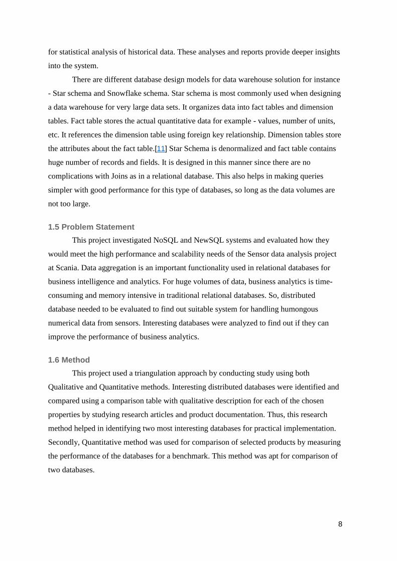
1.5 Problem Statement
This project investigated NoSQL and NewSQL systems and evaluated how they
would meet the high performance and scalability needs of the Sensor data analysis project
at Scania. Data aggregation is an important functionality used in relational databases for
business intelligence and analytics. For huge volumes of data, business analytics is time-
consuming and memory intensive in traditional relational databases. So, distributed
database needed to be evaluated to find out suitable system for handling humongous
numerical data from sensors. Interesting databases were analyzed to find out if they can
improve the performance of business analytics.
1.6 Method
This project used a triangulation approach by conducting study using both
Qualitative and Quantitative methods. Interesting distributed databases were identified and
compared using a comparison table with qualitative description for each of the chosen
properties by studying research articles and product documentation. Thus, this research
method helped in identifying two most interesting databases for practical implementation.
Secondly, Quantitative method was used for comparison of selected products by measuring
the performance of the databases for a benchmark. This method was apt for comparison of
two databases.

9
1.7 Limitations
This project was carried out for specific requirements of Sensor Data Analysis
project and hence, the Scope of the Qualitative comparison of distributed databases was
limited. All suitable databases were not taken into consideration for this study due to time
limitation and only few interesting databases from each category were considered. Also for
this reason, only two databases were selected for practical implementation.
1.8 Related work
Yahoo Cloud Serving Benchmark (YCSB) framework is a widely available, open
source benchmark for comparing NoSQL databases. YCSB generates load and compares
only read and write operations on the data. However, the performance of databases need to
be compared for data aggregation. Also, YCSB used high-performance hardware. Though
the framework is extensible, major changes were required for extending it to support data
aggregation. This was beyond the scope of the thesis due to time constraints and hence, a
simpler benchmark is developed for performance comparisons.
Altoros Systems performed a Vendor-independent comparison of NoSQL databases
Cassandra, HBase, Riak and MongoDB. These comparisons were done for only four
operations – read, insert, update and scan using YCSB.[12]
Paper [7] was a study of NoSQL databases to find out if NoSQL databases can
replace traditional databases for data aggregation. Above paper [7] compares relational
database and NoSQL database for aggregation which can be referenced but not used.
Comparisons among NoSQL databases is required for the sensor data analysis project.
Paper [13] was a study of the sensor data analysis project for optimization of data
warehouse solution conducted at Scania. Above paper [13] provided recommendations for
architecture and design of data warehouse solution. This solution is adapted and
implemented in the project. However, there are challenges in this system which were
investigated in this thesis.
Big data analytics is evolving and there are some systems that require realtime
query results. Storm is a scalable, reliable and distributed real time computation system. It
is used to perform realtime data analytics on unbounded streams. [14] An example use case
is twitter where updates are rapid and realtime business intelligence is required. Sensor data
problem does not require realtime data analytics since the writes are not very rapid. Also,
ad-hoc analyses performed on a week old data is acceptable.

10
2. Theory
2.1 Current System
The existing system uses data warehouse solution for sensor data analysis. [13] The
data is stored in Star Schema which is shown in Figure 1.
Figure 1 - Star Schema representation
Here, tables are organized into a fact table and several dimension tables. The fact
table contains all the data values which are the quantitative measurements and links to the
dimension tables. Dimension tables describe the data to allow meaningful analysis and are
related to the fact table. In this system, fact table is a huge data set containing millions of
rows.
2.2 Optimization of Schema design
In a relational database, table data is typically stored in local disk drives or network
storage and the indexes in random access memory using B-Tree or hash tree. [15] The
index provides quick access to data for read and write. The leaf nodes of the B-Trees have
pointers to data in secondary memory. Sensor data variables are stored in fact table and
attributes stored in dimension table. Each value of each attribute is stored in a separate row.
In such a solution, there are three dimensions of growth namely – 1. Number of Vehicles
grow, 2. Number of collected attributes grow and 3. Sampling rate grow by use of
Telemetry. Star schema is suboptimal in this case and leads to exponential growth. Each
Dimension Sample PK
descriptive attr1
descriptive attr2 descriptive attr3
PK descriptive attr1
descriptive attr2 descriptive attr3
DimensionChassi
PK descriptive attr1
DimensionVar
PK descriptive attr1 descriptive attr2
Dimension ECU
Fk1 Fk2 Fk3 Fk4
Value
Fact

11
snapshot of the sensor variable stores ‘N’ number of rows where ‘N’ denotes the length of
the array.
There are a number of drawbacks with the above schema design. First of all, growth
of data is rapid in three dimensions and will eventually lead to Scalability problems.
Secondly, reading data from one huge fact table can be very slow. This is because the
indexes are also huge and query performance is not boosted by indexes. Thirdly, in a big
table, rows will be spread out many disk blocks or memory segments. There is no
capability to store records of same variable together in a physical layout. If a variable is
represented as a separate small table, it’s possible that they may be stored together in disk
blocks. Also, indexing is quite fast for small tables. The entire table may be stored in
memory thereby greatly increasing performance.
Optimal schema for a Big Data solution needs many number of small tables instead
of a small number of huge tables. In the above case, if each sensor variable is stored in a
separate table indexed by primary key, the database will have better performance for ad
hoc queries. Partitioned table may give the same result. This is because the indexes are
effective for small tables.
2.3 Ideal database properties
To define ideal properties for a perfect solution for Sensor data, it is necessary to
understand the requirements of the system. In Scania, Sensor data is collected each time a
Vehicle enters the workshop. A Vehicle has many control units and each control unit has
many sensor variables. These control units accumulate value of the sensors. A variable can
have scalar, vector or matrix data type. Each sensor variable can have different versions
corresponding to different versions of control unit. Every time a control unit is replaced or
upgraded, each of its sensor variables could change having fewer or more values. Thus a
new version of each sensor variable is created for that control unit.
Sensor data is valuable for the company. They are used by BI Analysts to perform
various analyses to get deeper understanding of Vehicle component’s performance,
lifetime, technical problems, etc. The System is used for performing ad hoc analyses on the
historical data and to generate statistical reports. SAS tool is used as BI tool for generating
reports. The analyses are performed on a separate Server which holds a read only copy of
the data and hence the data is not realtime. The updates are performed on another Server
which is periodically copied into the BI Server.

12
Existing system is analyzed to understand the performance or scalability issues.
Future requirements of Sensor data project is gathered and analyzed. Considering the
purpose of the System, usage, and future requirements, the following properties are
identified as essential for a perfect solution.
● Scalability - The System should be able to scale-out horizontally by adding
additional nodes with as close as possible to linear scalability.
● High availability - The system may be integrated with online applications. It will be
a system running on a cluster of nodes (commodity hardware) and hence it is
important to be available always and tolerate failure of individual nodes.
● Elasticity - Elasticity is the representation of a system under load when new nodes
are added or removed. [7] If a system supports elasticity, then nodes can be added to
running system without shutting it down and it will automatically balances the load.
● High read performance - The database should have high throughput for sequential
and random read operations.
● High performance for computations - The system should have high performance for
computations such as calculating statistical median over the data set. Since the data
will be distributed, it should be possible to run algorithms or stored procedures on
the storage nodes locally to reduce required network bandwidth and to make
optimal use of the CPU capacity in the storage tier.
● Low Complexity - The System should be easy to use and maintain by programmers
through well documented APIs.
● Support data operations - The System should support create, read, and delete
operations on the data.
● Support by vendors or open source communities - The System should be well
documented and supported so that the database administrators and developers can
get support for product usage, bugs in the product, etc.
● Support for Indexes - Indexing helps in fast retrieval of data. We could relax this
criteria by designing a database that uses the primary index only if the system does
not support secondary indexes.
● Support for Business Intelligence tools - The database should be integrated with BI
tools to be able to generate statistical reports and graphs.
● Support for array or vector data type - It is desirable that the system support
collections like array or vector data type. This could help in improving the

13
performance of reads by accessing whole array or vector at once embedded in an
object and simplify programming.
● High throughput for bulk write or append for periodic updates
3. NoSQL databases
NoSQL is a collection of non-relational, typically schema-free databases designed
from scratch to address performance, scalability and availability issues of relational
databases for storing structured or unstructured data. There are different categories of
NoSQL databases. [10]
3.1 Column Families
Google’s BigTable inspired a class of column oriented data stores. HBase,
Cassandra, Amazon’s Dynamo, SimpleDB, Cloudata, Cloudera, Accumulo and
Stratosphere come under this category. [10] In traditional databases, if there are no values
for columns, null values are stored. Null values consume space though less than normal
data type. Column families have flexible number of columns in BigTable, and HBase. If
there are no values for a column, no values need to be stored and thus avoiding null values.
Hence for sparse data, they are efficient in usage of storage space. [16] In these databases,
each row is uniquely identified by a key. Thus each row is a key value pair and each
column is identified by the primary key and column family. Data is stored in a sorted and
sequential order. When the data exceeds the capacity of a single node, it is split and stored
into multiple nodes. The entire data set is in a single sorted sequence across nodes. Data
replication is provided by underlying distributed file system which also provides fault
tolerance of any storage nodes.
3.2 Document Store
Document stores denote a schema free storage where each document is
uniquely identified by a key. Here documents represented semi-structured data type like
JSON. Each document can be compared to a tuple in traditional relational databases.
Document can contain data of different types and structure known as properties. A
collection is comparable to a table in relational databases and contain a group of
documents. They support primary indexes through primary keys. Documents typically also

14
be indexed on any of their properties. There are many databases that fall into this category
– for instance MongoDB and Couch DB. [16]
3.3 Key Value
As the name suggests, this kind of databases have a set of key-value pairs where
key is unique and identifies a value. They can be quite efficient because a value typically
can be accessed in O (1) complexity similar to a Hash Map. There are three major types - 1.
Key stores based on Berkeley DB, 2. Memcached API key stores and 3. Key value store
built from scratch that do not belong to above two categories.
Berkeley DB has array of bytes for both keys and values. It does not have distinct
definition for key and values. Key and values can be of any data type. These keys can be
indexed for faster access. Memcached API has an in-memory storage of data identified by
unique keys. Memcached API is quite fast for reads and writes and are flushed to disks for
durability. Most key value stores provide APIs to get and set values. Redis is a highly
available key-value data stores which stores the data in memory. It is more of a data
structure server. The data types can be sets, maps, vectors and arrays. They provide rich
APIs for storing and retrieving data.
Riak is a distributed key value data store which provides very fast lookups and is
highly available. [17] It is written in Erlang and provides APIs in JSON. It can be quite
powerful since it provides strong guarantees using vector clocks.[10]
Amazon’s DynamoDB is a highly available key value stores which provides
reliability, performance and efficiency. Dynamo was built for high scalability and
reliability needs of Amazon’s e-commerce platform. It is built on fast solid state disks
(SSD) to support fast access to data. It supports automatic sharding, elasticity, and
provisioned capacity.[18]
3.4 Graph databases
This category of databases uses graph structures to store data. They have nodes,
edges and properties to represent data. Most graph databases do not have indexes because
each node has pointer to adjacent element and hence provide faster access for graph-like
queries. Real world objects such as Product ratings, Social networks can be easily designed
using these databases and provide fast read or write access. There are several graph
databases in the market - Neo4j, HyperGraphDB, GraphBase, BigData, etc. Neo4j is a

15
popular graph database that is widely used to design, for instance product catalogs and
databases which change frequently.
3.5 Multimodel databases
According to Matthew Aslett [5], these are the databases that are built specially for
multiple data models. FoundationDb is a database that supports key-value data model,
document layer and object layer. Riak is a highly available key value store where the value
can be a JSON document. Couchbase database supports document layer and key-value data
layer. OrientDB is a document sore which supports object layer as well as graph data layer.
3.6 Object databases
Databases such as ZopeDB, DB40, and Shoal are object oriented databases.
ZopeDB stores python objects. DB40 is a schema free object database that supports storage
and retrieval of .Net and Java objects. Shoal is an open source cluster framework in Java.
These databases provide efficient storage and retrieval of data as objects. However, they
are not widely adopted because these databases are tied to object model of respective
programming languages and lack standard query language like SQL. So they are dependent
on specific language limitations which is a major drawback.
3.7 Grid and Cloud databases
Grid and Cloud databases provide data structures that can be shared among the
nodes in a cluster and distribute workloads among the nodes. Hazelcast [19] is an in-
memory data grid that provides shared data structures in Java and distributed cache. It also
provides JAAS based security framework which secures read or write client operations and
authenticates requests. Oracle Coherence is an in-memory distributed data grid and is used
at Scania.
Infinispan is a highly available, scalable, open source data grid platform written in
Java.[20] It supports shared data structure that is highly concurrent and provides distributed
cache capabilities. It maintains state information among the nodes through a peer to peer
architecture. GigaSpaces provides an in-memory data grid and a data store in the cloud
through Cloudify. GigaSpaces supports NoSQL frameworks such as couchbase, Hadoop,
Cassandra, Rails, MongoDB, and SQL frameworks such as MySQL in the Cloud. [21] It
provides support for both private and public cloud.

16
GemFire is also an in-memory distributed data management framework which is
scalable dynamically and gives very good performance. It is built using spring framework
and provides low latency by avoiding delays due to network transfer and disk I/O. [22]
3.8 XML databases
XML databases either stores data in XML format or supports XML document as
input and output to the database. If the data is stored in XML format, XPath and XQuery
are typically used to query the data in the documents. These databases are also known as
document-centric databases.
Some of the popular XML databases are EMC document xDB, eXist, BaseX, sedna,
QizX and Berkeley DB XML. BaseX is a lightweight, powerful open source XML
database written in Java. It is fully indexed, scalable and provides support for version 3.0 of
XPath or XQuery for querying. It has a client-server architecture and guarantees ACID
properties for datastore. It can store small number of very large XML documents where
each document can be several Gigabytes. eXist is an open source schema-free XML
database which can store binary and textual data.
4. NewSQL databases
NewSQL databases address scalability, performance and availability issues of
relational DBMS and provide full or partial SQL query capability. Most of them follow
relational data model. There are four categories of NewSQL databases namely – 1. New
databases, 2. Database-as-a-service, 3.Storage engines, and 4. Clustering or sharding.[23]
4.1 New databases
These are a kind of relational databases that are recently developed for horizontal
scalability, high performance and availability. Some of the popular databases under this
category are as follows – NuoDB, VoltDB, MemSQL, JustOneDB, SQLFire, Drizzle and
Akiban Translattice. NuoDB is described in detail in the following section to give an idea
about this category.
4.1.1 NuoDB
This is a scalable, high performance cloud data management system that is capable
of being deployed in cloud or in data center.[24] It has a three tier deployment architecture.
Cloud, data center or hybrid deployment form the first tier. Operating system such as

17
Linux, Windows and MacOS form the second tier. Third tier has NuoDB components,
namely - Broker, Transaction Engine, Storage Manager (SM), and File system.
Each of the components is run as an in-memory process running on hosts. SM is
responsible for persisting data and retrieving it. Broker is responsible for providing access
to database for external applications. Transaction Engine is responsible for handling
transactions. It retrieves data from its peers when required. So data is stored durably in SM
and replicated to Transaction engine when needed. When a Transaction engine is created it
learns the topology and acquires metadata from its peers. For scalability new NuoDB
processes can be added. When a SM is added, it receives a copy of entire database for
reliability and performance.
All client requests are handled by Transaction engine which runs a SQL layer.
NuoDB also supports other frameworks such .Net, Java, Python, Perl and PHP. SM
supports handling data in a distributed file system such as HDFS, Amazon S3 or SAN or
regular file system. Since transaction handling is separated from data storage it is able to
provide very good performance for concurrent reads and writes. An important feature of
this product is that it is capable of providing realtime data analytics. Also it has capability
to run in geographically distributed data center and hence it is possible to take application
global.
4.2 Database-as-a-Service
Traditional DBMS are not suited to be run in a Cloud environment. So Database
services emerged to address this issue and to adapt DBMS to be run on public or private
cloud. These are the Cloud Database services which are deployed using Virtual machines.
NuoDB, MySQL, GaianDB and Oracle database can be deployed in cloud. Another data
model for database in cloud is Database-as-a-Service.
These solutions provide database software and physical storage with sensible out of
box settings. No installation or configuration is required to start such a service which is an
on-demand, pay-per-usage service. The Service provider is fully responsible for
maintaining the service, upgrading and administering the database.[25] For instance
Microsoft SQL Azure, StormDB, ClearDB and EnterpriseDB belong to Database-as-a-
service category. StormDB is described in detail to give an overview of this category.
4.2.1 StormDB
StormDB is a distributed database that is fully managed in cloud. It can be created
and accessed as a service through a browser. It differs from regular cloud databases by

18
running the database instance on bare metal instead of running it in a virtual environment.
This helps in providing scalability of the system. It has a feature called Massively Parallel
Processing (MPP) through which it process even complex queries and data analytics over
entire data set very quickly (in seconds). It is a relational database supporting high volume
of OLTP reads and writes. It supports transaction handling and is ACID compliant. It is
based on PostgreSQL and hence provides SQL interface. It also supports many other APIs
such as .Net, Java, Python, Ruby, Erlang, C++, etc. There is no installation or deployment
to be done by customers. StormDB instances can be created very easily and are fully
managed by the Vendor. It has all the advantages of NewSQL databases and is also very
easy to use.[26]
4.3 Storage engines
MySQL is an OLTP database that is fully ACID compliant and handles transactions
efficiently. However, it has scalability and performance limitations. One solution to this
problem is sharding of data but this may result in consistency issues and is complicated to
handle at application level. When data is partitioned among servers, all the copies have to
be maintained consistently and there may be complications while handling transactions.
Hence alternative storage engines have been developed to address the scalability and
performance problems. MySQL NDB Cluster is a popular storage engine that is being
widely used today. Other storage engines are Xeround, GenieDb, Tokutek and Akiban.
MySQL Cluster is described in detail in Section 9.
4.4 Clustering or Sharding
Some SQL solutions introduce pluggable feature to address scalability limitations.
Some solutions shard data transparently to address scalability issue. Examples of this
category are Schooner MySQL, Tungsten, ScaleBase, ScalArc and dBShards.
5. Comparative study
A Qualitative method is used to identify interesting products. Thus a study of
different NoSQL and NewSQL products is carried out using research articles, academic
papers, product documentation and community forums. A comparison of interesting
NoSQL and NewSQL databases is carried out against desired properties for a storage
solution. The comparison is listed in table below.

19
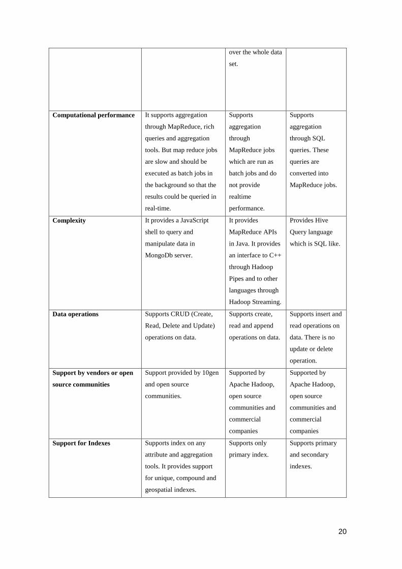
5.1 Comparison of NoSQL Databases – MongoDb, Hadoop, Hive
Criteria MongoDb Hadoop Hive
Description It is a document oriented
data store designed to scale
out.
It is an open source
framework that
supports
processing of
massive data sets
using a distributed
computational
cluster.
It is a data
warehousing
framework built on
top of Hadoop.
Scalability It automatically distributes
data and load across
multiple servers.
Scales horizontally
and supports auto
sharding.
It scales linearly
and supports auto
sharding.
Availability Supports high availability
through asynchronous
replication
High availability
provided by
Hadoop
Distributed File
System (HDFS)
and YARN.
High availability
provided by
HDFS.
Elasticity New nodes can be added or
removed online. [27]
New nodes can be
added or removed
dynamically.
New nodes can be
added or removed
dynamically.
Read performance It supports high read
performance through
memory-mapped files.
It is not suited for
random reads and
low latency reads
since each read
operation is a scan
It provides better
read performance
than Hadoop
because of primary
and secondary
indexes.
20
over the whole data
set.
Computational performance It supports aggregation
through MapReduce, rich
queries and aggregation
tools. But map reduce jobs
are slow and should be
executed as batch jobs in
the background so that the
results could be queried in
real-time.
Supports
aggregation
through
MapReduce jobs
which are run as
batch jobs and do
not provide
realtime
performance.
Supports
aggregation
through SQL
queries. These
queries are
converted into
MapReduce jobs.
Complexity It provides a JavaScript
shell to query and
manipulate data in
MongoDb server.
It provides
MapReduce APIs
in Java. It provides
an interface to C++
through Hadoop
Pipes and to other
languages through
Hadoop Streaming.
Provides Hive
Query language
which is SQL like.
Data operations Supports CRUD (Create,
Read, Delete and Update)
operations on data.
Supports create,
read and append
operations on data.
Supports insert and
read operations on
data. There is no
update or delete
operation.
Support by vendors or open
source communities
Support provided by 10gen
and open source
communities.
Supported by
Apache Hadoop,
open source
communities and
commercial
companies
Supported by
Apache Hadoop,
open source
communities and
commercial
companies
Support for Indexes Supports index on any
attribute and aggregation
tools. It provides support
for unique, compound and
geospatial indexes.
Supports only
primary index.
Supports primary
and secondary
indexes.
21
Support for Business
Intelligence tools
It can be easily integrated
with pentaho
supports pentaho supports pentaho
Support for array or vector
data type
Supports arrays and
embedded documents.
Supports custom
data types in Java.
Supports arrays
and complex data
types.
High throughput for bulk
inserts
Provides built-in support
for bulk inserts and hence
High throughput is possible
for bulk loading.
High throughput
for bulk insert is
supported since
they are executed
as MapReduce
jobs.
High throughput
for bulk insert is
supported.
Table 1 - Comparison of NoSQL Databases: MongoDB, Hadoop and Hive
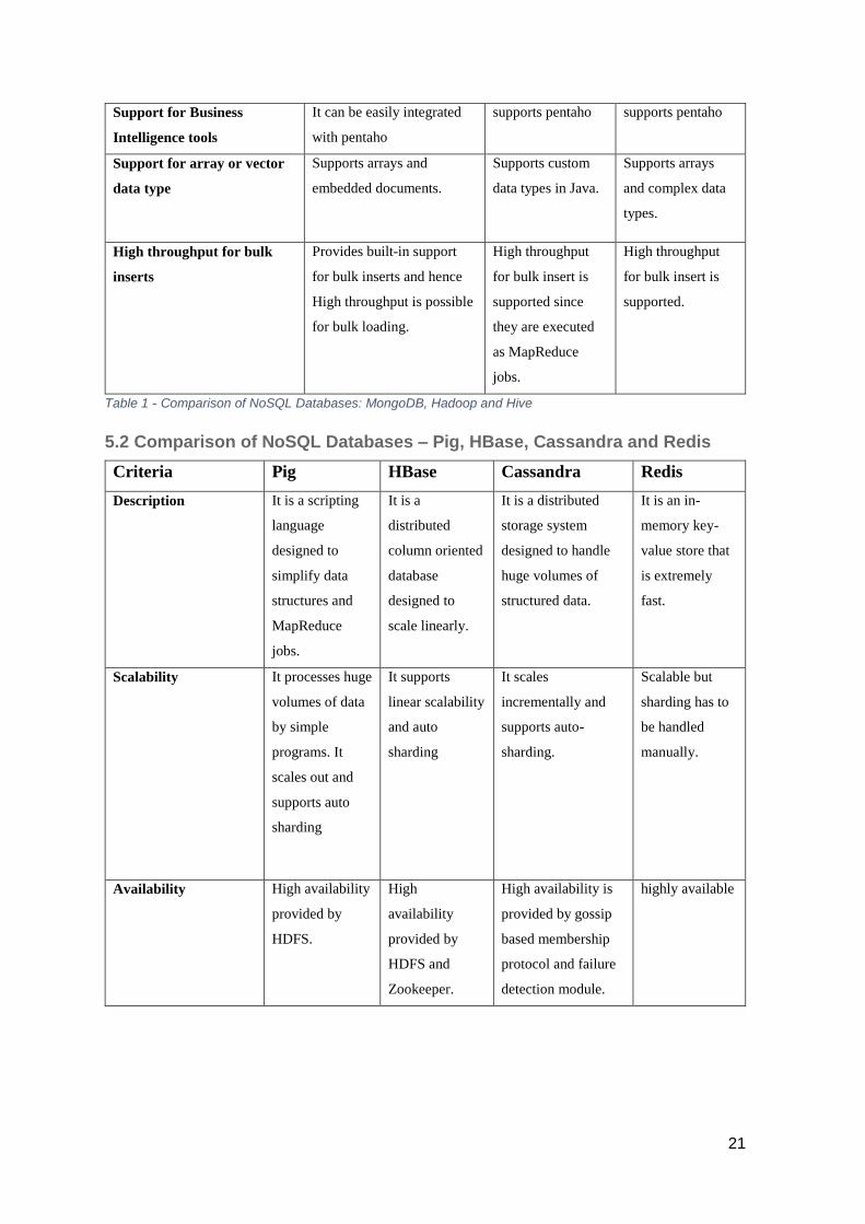
5.2 Comparison of NoSQL Databases – Pig, HBase, Cassandra and Redis
Criteria Pig HBase Cassandra Redis
Description It is a scripting
language
designed to
simplify data
structures and
MapReduce
jobs.
It is a
distributed
column oriented
database
designed to
scale linearly.
It is a distributed
storage system
designed to handle
huge volumes of
structured data.
It is an in-
memory key-
value store that
is extremely
fast.
Scalability It processes huge
volumes of data
by simple
programs. It
scales out and
supports auto
sharding
It supports
linear scalability
and auto
sharding
It scales
incrementally and
supports auto-
sharding.
Scalable but
sharding has to
be handled
manually.
Availability High availability
provided by
HDFS.
High
availability
provided by
HDFS and
Zookeeper.
High availability is
provided by gossip
based membership
protocol and failure
detection module.
highly available

22
Elasticity New nodes can
be added online
but data will be
distributed from
the old nodes to
the new nodes
and it takes time
before new
nodes start
serving requests.
When new
nodes are added
dynamically,
there is no big
data transfer
from the old
nodes to new
nodes and hence
the new node
start serving
requests
immediately.
New nodes can be
added online but
data will be
distributed from the
old nodes to the new
nodes and it takes
time before new
nodes start serving
requests.[27]
Adding or
removing nodes
is complex and
takes lot of time
since hash slots
will be moved
around.
Read performance It is slower than
Java MapReduce
programs and
hence
performance is
slower than
Hadoop.
Rows are sorted
by primary key
and hence
supports low
latency for
sequential and
random reads.
It uses in-memory
structure called
bloom filters which
is like a cache and is
checked first for
read requests. Hence
it provides good read
performance.
It is more of a
cache since it
stores data in
memory and
hence it’s quite
fast for random
reads and
writes.
Computational
performance
Supports
MapReduce
functionality.
Supports
aggregation
through
MapReduce
Jobs.
Support for
MapReduce is not
native and is slower
than Hadoop.
Although it can be
used along with
Storm for real time
computation.
Provides fast
real time
analytics.
Complexity It provides a
level of
abstraction
through APIs
and simplifies
MapReduce
programming.
Provides a shell
with simple
commands to
perform
querying and
manipulating
data.
Provides Cassandra
Query Language
(CQL), command-
line interfaces and
APIs.
Provides APIs
but no ad hoc
querying
feature.
Data operations Supports create,
read and append
operations on
data.
Supports create,
read and append
operations on
data.
Supports CRUD
operations on data.
Supports CRUD
operations on
data.

23
Support by vendors or
open source
communities
Supported by
Apache Hadoop,
open source
communities and
commercial
companies
Supported by
Apache
Hadoop, open
source
communities
and commercial
companies
Supported by open
source communities
Supported by
open source
communities
and commercial
companies
Support for Indexes Supports only
primary index
Supports
primary index
efficiently.
Although
secondary
indexing is
possible, it is
not effective.
Supports primary
and secondary
indexes.
Supports only
primary index.
Support for Business
Intelligence tools
Supports
pentaho
Supports
pentaho
Supports pentaho BI supported by
sysvine
Support for array or
vector data type
Supports Arrays
and complex
data types such
as tuples, bags
and maps.
Supports custom
data types in
Java.
Supports custom
data types.
Supports
complex data
types like
hashes, lists and
sets.
High throughput for
bulk inserts
High throughput
for bulk inserts
is supported.
High throughput
for bulk insert is
supported since
they are
executed as
MapReduce
jobs.
High throughput for
bulk inserts is
supported.
High throughput
for bulk inserts
is supported.
Table 2 - Comparison of NoSQL Databases: Pig, HBase, Cassandra and Redis
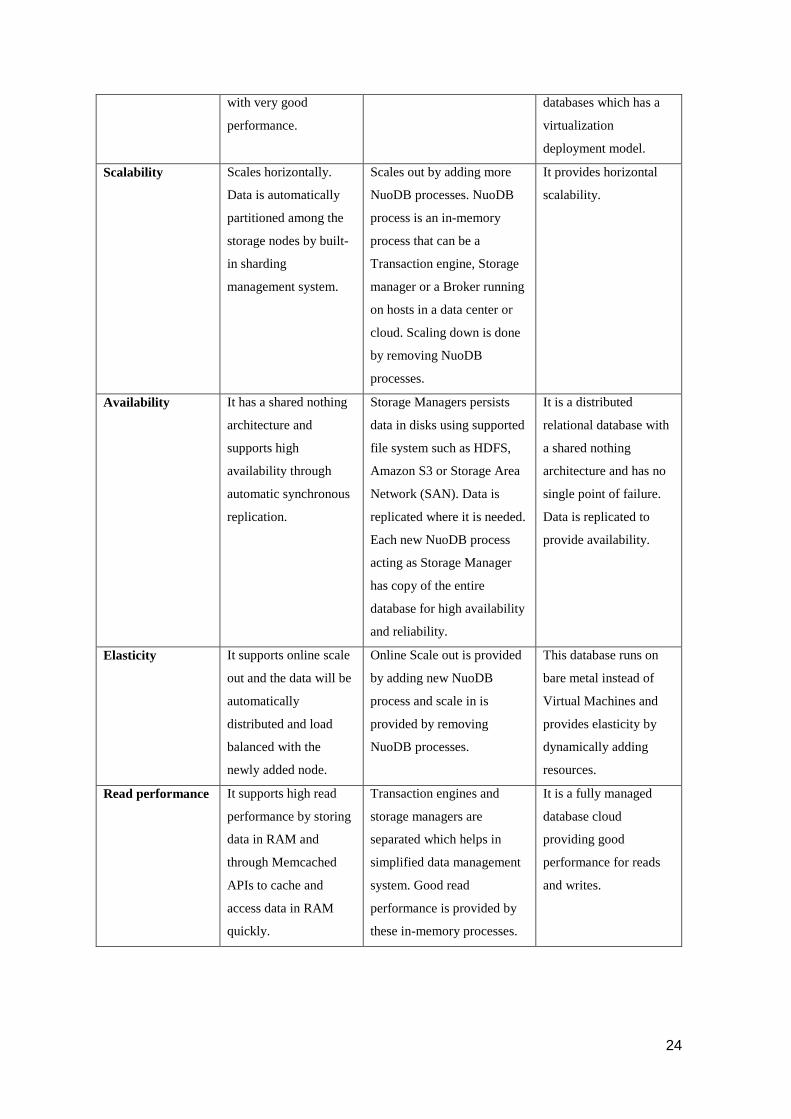
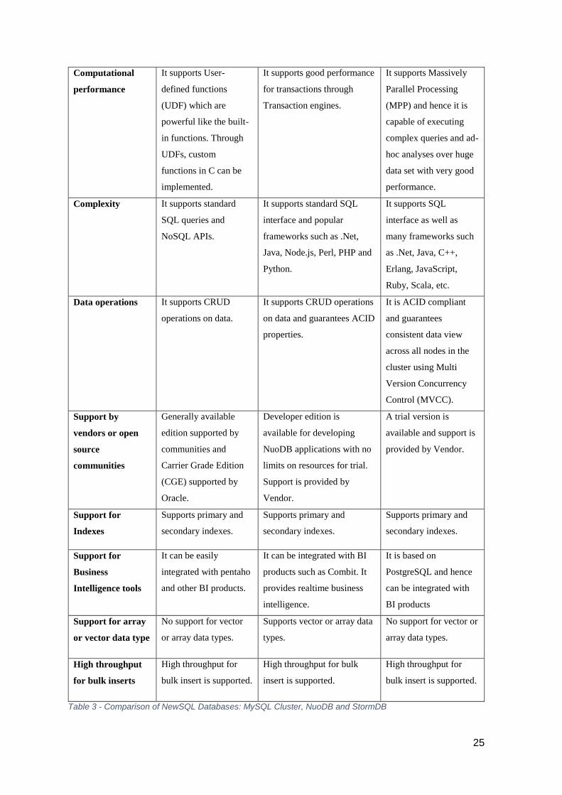
5.3 Comparison of NewSQL Databases – MySQL Cluster, NuoDB and
StormDB
Criteria MySQL Cluster NuoDB StormDB
Description MySQL NDB Cluster
is a storage engine
designed to scale out
It is a relational database in
cloud that is ACID compliant
and provides SQL query
capability.
StormDB is a Database
Cloud running on bare
metal unlike
conventional cloud
24
with very good
performance.
databases which has a
virtualization
deployment model.
Scalability Scales horizontally.
Data is automatically
partitioned among the
storage nodes by built-
in sharding
management system.
Scales out by adding more
NuoDB processes. NuoDB
process is an in-memory
process that can be a
Transaction engine, Storage
manager or a Broker running
on hosts in a data center or
cloud. Scaling down is done
by removing NuoDB
processes.
It provides horizontal
scalability.
Availability It has a shared nothing
architecture and
supports high
availability through
automatic synchronous
replication.
Storage Managers persists
data in disks using supported
file system such as HDFS,
Amazon S3 or Storage Area
Network (SAN). Data is
replicated where it is needed.
Each new NuoDB process
acting as Storage Manager
has copy of the entire
database for high availability
and reliability.
It is a distributed
relational database with
a shared nothing
architecture and has no
single point of failure.
Data is replicated to
provide availability.
Elasticity It supports online scale
out and the data will be
automatically
distributed and load
balanced with the
newly added node.
Online Scale out is provided
by adding new NuoDB
process and scale in is
provided by removing
NuoDB processes.
This database runs on
bare metal instead of
Virtual Machines and
provides elasticity by
dynamically adding
resources.
Read performance It supports high read
performance by storing
data in RAM and
through Memcached
APIs to cache and
access data in RAM
quickly.
Transaction engines and
storage managers are
separated which helps in
simplified data management
system. Good read
performance is provided by
these in-memory processes.
It is a fully managed
database cloud
providing good
performance for reads
and writes.
25
Computational
performance
It supports User-
defined functions
(UDF) which are
powerful like the built-
in functions. Through
UDFs, custom
functions in C can be
implemented.
It supports good performance
for transactions through
Transaction engines.
It supports Massively
Parallel Processing
(MPP) and hence it is
capable of executing
complex queries and ad-
hoc analyses over huge
data set with very good
performance.
Complexity It supports standard
SQL queries and
NoSQL APIs.
It supports standard SQL
interface and popular
frameworks such as .Net,
Java, Node.js, Perl, PHP and
Python.
It supports SQL
interface as well as
many frameworks such
as .Net, Java, C++,
Erlang, JavaScript,
Ruby, Scala, etc.
Data operations It supports CRUD
operations on data.
It supports CRUD operations
on data and guarantees ACID
properties.
It is ACID compliant
and guarantees
consistent data view
across all nodes in the
cluster using Multi
Version Concurrency
Control (MVCC).
Support by
vendors or open
source
communities
Generally available
edition supported by
communities and
Carrier Grade Edition
(CGE) supported by
Oracle.
Developer edition is
available for developing
NuoDB applications with no
limits on resources for trial.
Support is provided by
Vendor.
A trial version is
available and support is
provided by Vendor.
Support for
Indexes
Supports primary and
secondary indexes.
Supports primary and
secondary indexes.
Supports primary and
secondary indexes.
Support for
Business
Intelligence tools
It can be easily
integrated with pentaho
and other BI products.
It can be integrated with BI
products such as Combit. It
provides realtime business
intelligence.
It is based on
PostgreSQL and hence
can be integrated with
BI products
Support for array
or vector data type
No support for vector
or array data types.
Supports vector or array data
types.
No support for vector or
array data types.
High throughput
for bulk inserts
High throughput for
bulk insert is supported.
High throughput for bulk
insert is supported.
High throughput for
bulk insert is supported.
Table 3 - Comparison of NewSQL Databases: MySQL Cluster, NuoDB and StormDB

26
Among the databases, two most interesting databases are selected, one from each
category for practical implementation and evaluation. The decision about interesting
databases is made by giving more weightage to computational performance criteria and
availability for practical implementation. Some of the NewSQL databases need to be
purchased before any development can be done.
HBase stands out among the NoSQL databases because of following reasons – 1. It
has tight integration with MapReduce framework and hence provides high performance for
computations, 2. It provides high throughput for reads through caching and filters, and 3. It
is available as open source and hence can be easily deployed without any licensing issues.
Also, support is provided by open source communities.
MySQL Cluster is chosen among the NewSQL databases because of following
reasons – 1. Community edition is available for development, 2. It provides good
computational performance through UDFs and NDB C++ APIs.
6. Polyglot Persistence
Each category of databases address a specific storage problem. No single storage
solution can be a perfect solution for all use cases. There are limitations on each category.
It is essential to understand the features and limitations of each database. According to
Martin Fowler [28], a complex application requires a combination of database products to
solve the storage problem. More than one database product is used to store and manipulate
data. This is known as polyglot persistence. Figure 2 shows an example of polyglot
persistence. It shows a web application for retail management. The storage uses Apache
Hadoop and Cassandra for data analytics and user activity logs respectively.

27
Figure 2 - A Speculative retailer’s web application. *Adapted from Martin Fowler page [28]
7. HBase
7.1 Overview
HBase is a column family oriented data store designed to store very large tables. It
is modeled after Google’s Bigtable. It is a multidimensional data store supporting
versioned data. It provides random read or write access to data. It is built for high
availability, scalability and good performance. Analytics on massive data sets is supported
by HBase using Parallel programming model known as MapReduce framework. HBase
does batch processing on massive data sets by pushing computations to the data nodes
through MapReduce tasks.

28
7.2 File System
HBase requires a distributed file system storage for storing data and performing
computations. Hadoop Distributed File System (HDFS) is the commonly used distributed
file system for HBase in production. HDFS is designed for storing very large data sets.
These files are primarily of type write once and read many times. Data is written at the end
of the file and the file system doesn’t support modifications. HDFS stores information
about the files called metadata in Name node. Application data is stored in data nodes.
When a client requests a data block, it is looked up in the Name node and redirected
to the corresponding data node. The data node performs the function of retrieving and
storing data blocks. The data nodes periodically update the Name node with metadata of
data blocks it contains. This Meta data is persistently stored in a namespace image and edit
log. If the Name node fails, the file system will be unstable. Hadoop provides fault
tolerance of Name node through a Secondary name node. This is a separate node which
periodically merges its namespace image with the edit log. This eliminates the possibility
of the edit log becoming too large. The Secondary name node also saves the merged
namespace image. Recent versions of Hadoop provide YARN a resource manager which
provides fault tolerance for Namenode. An overview of HDFS is pictographically
represented in the Figure 3.
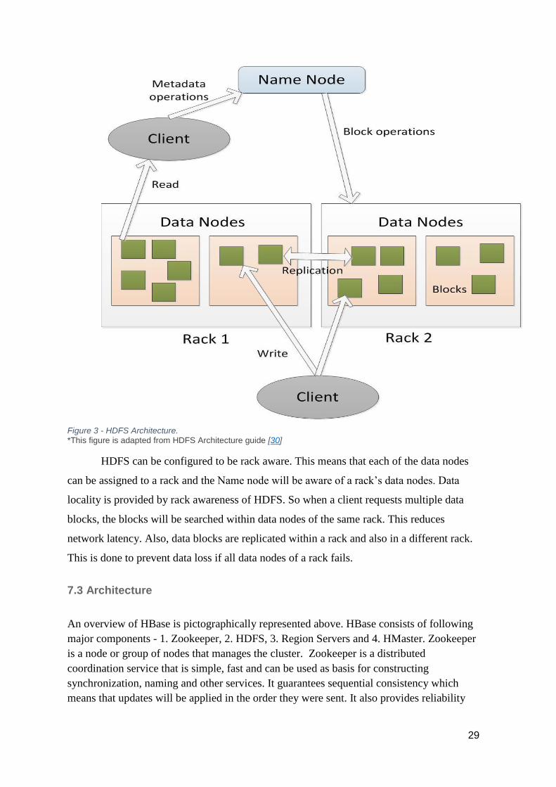
Metadata is stored in memory in the Name node. The total number of files
in file system is limited by the size of main memory in the Name node. Hence, the design
supports storing small number of large files. Each file is divided into many data blocks and
stored in a data node in the cluster. The data blocks are of fixed size. The data block is a
unit of abstraction rather than a file. This makes the file system simple by dealing with
replication or failure management. Replication of data blocks provide high availability in
case of failure of any data node in the cluster. Each data block is larger in size than the
usual disk block. It is because time to seek to start of the block will be significantly smaller
than the time to transfer a data block. Hence data transfer of a large file will be at the disk
transfer rate. [29]
29
Figure 3 - HDFS Architecture. *This figure is adapted from HDFS Architecture guide [30]
HDFS can be configured to be rack aware. This means that each of the data nodes
can be assigned to a rack and the Name node will be aware of a rack’s data nodes. Data
locality is provided by rack awareness of HDFS. So when a client requests multiple data
blocks, the blocks will be searched within data nodes of the same rack. This reduces
network latency. Also, data blocks are replicated within a rack and also in a different rack.
This is done to prevent data loss if all data nodes of a rack fails.
7.3 Architecture
An overview of HBase is pictographically represented above. HBase consists of following
major components - 1. Zookeeper, 2. HDFS, 3. Region Servers and 4. HMaster. Zookeeper
is a node or group of nodes that manages the cluster. Zookeeper is a distributed
coordination service that is simple, fast and can be used as basis for constructing
synchronization, naming and other services. It guarantees sequential consistency which
means that updates will be applied in the order they were sent. It also provides reliability
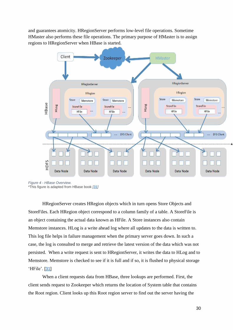
30
and guarantees atomicity. HRegionServer performs low-level file operations. Sometime
HMaster also performs these file operations. The primary purpose of HMaster is to assign
regions to HRegionServer when HBase is started.
Figure 4 - HBase Overview. *This figure is adapted from HBase book [31]
HRegionServer creates HRegion objects which in turn opens Store Objects and
StoreFiles. Each HRegion object correspond to a column family of a table. A StoreFile is
an object containing the actual data known as HFile. A Store instances also contain
Memstore instances. HLog is a write ahead log where all updates to the data is written to.
This log file helps in failure management when the primary server goes down. In such a
case, the log is consulted to merge and retrieve the latest version of the data which was not
persisted. When a write request is sent to HRegionServer, it writes the data to HLog and to
Memstore. Memstore is checked to see if it is full and if so, it is flushed to physical storage
‘HFile’. [31]
When a client requests data from HBase, three lookups are performed. First, the
client sends request to Zookeeper which returns the location of System table that contains
the Root region. Client looks up this Root region server to find out the server having the
31
Meta region of the requested row keys. This information is cached and performed only
once. Then the client looks up this Meta region server to find out the region server that
contains the requested row keys. Then the client directly queries this region server to
retrieve the user table.
A background thread in HBase monitors store files so that the HFiles do not
become too many in numbers. They are merged to produce few large files. This process is
known as compaction. There are two types of compactions - minor and major. Major
compactions merges all files into a single file whereas minor compactions merge the last
few files into larger files.
While designing an HBase database, it is recommended to have few column
families typically 2 or 3. This is because flushing and compaction happens region wise. So
if there are many column families, flushing and compaction will require a lot of I/O
processing. Also, if a column family has large amount of data while another column family
has little data but both will be flushed if they are in the same region.
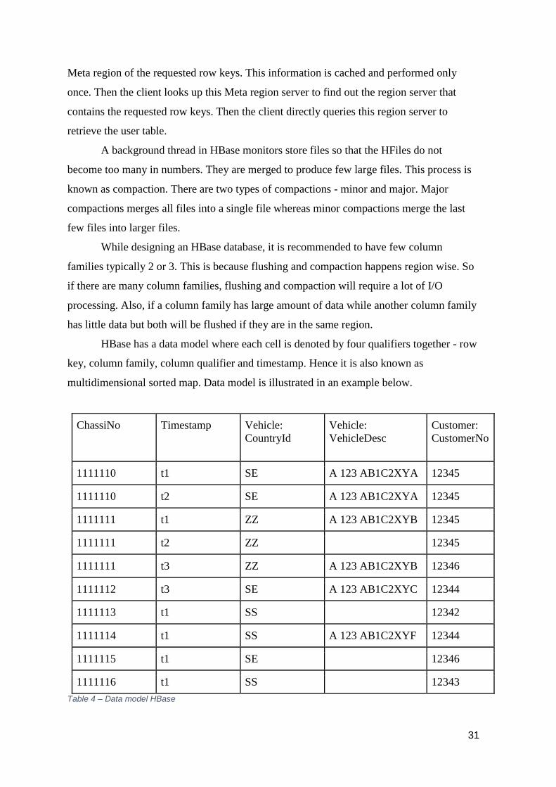
HBase has a data model where each cell is denoted by four qualifiers together - row
key, column family, column qualifier and timestamp. Hence it is also known as
multidimensional sorted map. Data model is illustrated in an example below.
ChassiNo Timestamp Vehicle:
CountryId
Vehicle:
VehicleDesc
Customer:
CustomerNo
1111110 t1 SE A 123 AB1C2XYA 12345
1111110 t2 SE A 123 AB1C2XYA 12345
1111111 t1 ZZ A 123 AB1C2XYB 12345
1111111 t2 ZZ 12345
1111111 t3 ZZ A 123 AB1C2XYB 12346
1111112 t3 SE A 123 AB1C2XYC 12344
1111113 t1 SS 12342
1111114 t1 SS A 123 AB1C2XYF 12344
1111115 t1 SE 12346
1111116 t1 SS 12343
Table 4 – Data model HBase

32
With Column families a column can either have value or no value. Thus it saves
space in storing null value for a column. This is significant in a massive data table where
there is a huge number of null values. In the above example, vehicleDesc column does not
have a value for some rows. Also same row key can have multiple versions based on
timestamp as shown above.
7.4 Features
Major features of HBase is described below
● Caching
HBase provides LRU cache functionality known as block cache which
caches frequently used data blocks. There are three types of block priority - 1.
Single access, 2. Multiple access and 3. In-memory. When a block is accessed for
the first time, it will be in 1st category and will be upgraded to 2nd category when it
is accessed again. In-memory blocks will be kept in memory, set by database
administrators.
Block cache also caches catalog tables such as .META and .ROOT, HFile
indexes and keys. Block cache should be turned off for Map reduce programs
because when using the Map reduce Framework, each table is scanned only once.
Also, block cache should be turned off for totally random read access. In other
cases, block cache should be enabled so that the Region servers do not spend
resources loading indices over and over. [32]
● Filters
In HBase, rows can be retrieved using scan functionality by column family,
column qualifier, key, timestamp, and version number. A Filter will improve read
effectiveness by adding functionality to retrieve keys or values based on regular
expressions. There are many predefined filters and it is also easy to implement user
defined filter by extending base filter class.
HBase provides Bloom filters for column families. Bloom filter is a
functionality which checks if a specific row key is present in a StoreFile or not.
There could be false positive where in a check returns true while the row key is not
present in the StoreFile. This parameter can be tuned drastically reducing the time
to seek a random row key.
● Autosharding
Regions store contiguous rows of data. Initially, there will be only one region.

33
When the rows become larger than the configured maximum size, it is split into two
regions. Each region is served by only one region server and a region server can
serve many regions. When a region server serving a region becomes loaded, then
the regions are moved between servers for load balancing. This splitting and
serving of regions is known as Autosharding and is handled by framework. [31]
● Automatic failover for region server
when a region server fails, then the client requests are automatically redirected to
other region servers serving the regions.
● Consistency
HBase guarantees some level of consistency. Updates made at row level are atomic.
However, it does not guarantee ACID properties.
● MapReduce
HBase provides support for a MapReduce framework which is described in detail in
the following section.
7.5 MapReduce Framework
MapReduce is a simple but powerful parallel programming framework through
which computations are performed locally on storage nodes. Since computations are
performed locally, network latency for data transfer may be reduced. Also, the processing
power on each of the storage nodes is utilized. Hence it has a capability to perform data
analytics on very large data sets using commodity hardware. An overview of MapReduce
framework is represented in Figure 5 - An overview of MapReduce Framework.
In MapReduce framework, the input is a very large data file or binary file which is
split into parts. The input is split in such a manner to take advantage of the available
number of servers and other infrastructure. MapReduce job is designed to scale
horizontally with addition of more servers. In this framework, there are two types of tasks -
map tasks and reduce tasks. The purpose of a map task is to take an input split which can
be a file split or table rows and transform them into intermediate key-value pairs. These
key value-pairs are grouped using a sort-merge algorithm, shuffled and sent to the reducers.
The purpose of reduce tasks are to aggregate the key-value pairs using user-defined reduce
function and produce the results.

34
Figure 5 - An overview of MapReduce Framework. *This figure is adapted from Paper. [33]
According to Herodotos [33], there are five phases in map task - read, map, collect,
spill, and merge. In the read phase, input split is read from HDFS and key-value pairs are
created. In the map phase, user-defined map function is executed on the key-value pairs. In
the collect phase, these intermediate key-value pairs are partitioned and collected into a
buffer. In the spill phase, the intermediate values are sorted using combine function if
specified and then they are compressed if this is configured. Output is written to file spills.
Finally, file spills are merged into a map output file.
In reduce task [33], there are four phases - shuffle, merge, reduce, and write. In the
shuffle phase, intermediate data from map tasks are transferred to reducers and
decompressed if required. Then the intermediate values are merged and a user-defined
reduce function is executed to aggregate the key-value pairs that are written to HDFS.
In HBase, there is a Master - Slave architecture. The job tracker acts as a Master
and splits input data into many data splits and assigns them to task trackers based on data
locality for map tasks. A task tracker takes the input split and maps the input values into
intermediate key-value pairs. So a table input split is taken as input for map task and key-
value pairs are output into a temporary file in HDFS. The location of these temporary files
35
are sent to a job tracker which in turn sends it to the scheduled task trackers responsible for
the reduce task. These temporary files are transferred to corresponding reducers.
Job tracker monitors the task trackers and the task trackers send status to Job
tracker. Job tracker runs backup tasks based on speculative estimation to provide fault
tolerance of task trackers. The number of mappers and reducers can be configured using
MapReduce API.
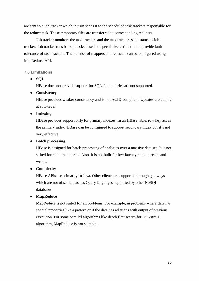
7.6 Limitations
● SQL
HBase does not provide support for SQL. Join queries are not supported.
● Consistency
HBase provides weaker consistency and is not ACID compliant. Updates are atomic
at row-level.
● Indexing
HBase provides support only for primary indexes. In an HBase table, row key act as
the primary index. HBase can be configured to support secondary index but it’s not
very effective.
● Batch processing
HBase is designed for batch processing of analytics over a massive data set. It is not
suited for real time queries. Also, it is not built for low latency random reads and
writes.
● Complexity
HBase APIs are primarily in Java. Other clients are supported through gateways
which are not of same class as Query languages supported by other NoSQL
databases.
● MapReduce
MapReduce is not suited for all problems. For example, in problems where data has
special properties like a pattern or if the data has relations with output of previous
execution. For some parallel algorithms like depth first search for Dijikstra’s
algorithm, MapReduce is not suitable.
36
8. MySQL Cluster
MySQL Cluster is a highly available database that can scale well for both reads and writes
with good performance. It belongs to NewSQL category and is a relational database that is
built ground up for high scalability. It is ACID compliant and provides support for SQL
and indexes. It also supports access to database through NOSQL APIs, Memcached APIs
and native APIs. It has a shared-nothing, distributed, multi-master architecture with no
single point of failure. It is best suited for low latency access and high volume of writes. It
can be an in-memory datastore for low-latency access or it can be configured to also use
disk storage.
8.1 Overview
The architecture of MySQL Cluster is represented in Figure 6. There is two tiers of
nodes - Storage tier and SQL Server tier. There is a cluster manager node which is
responsible for cluster management and configuration. The Storage tier contain data nodes
which are responsible for data storage and retrieval. SQL Server nodes are the application
nodes which provide access to data through SQL and NoSQL APIs like REST or HTTP,
Memcached APIs, JPA or C++. [34]
Data nodes are organized into node groups. Data is automatically partitioned (Auto-
sharding) by the database layer. The Data shards are stored in a data node and the
partitioning is based on hashing of primary key. Thus the data shards are distributed evenly
using a hashing function thereby handling the load balancing of data nodes. The data
shards are replicated in such a manner that it is present in data nodes of different node
groups to prevent data loss when a node group goes down. Replication factor can be
configured in the cluster manager node. Data replication provides high availability and
fault tolerance.
When a read requests is sent from an application, it is handled by one of the
application nodes. The application node queries and retrieves the requested rows from data
nodes. It is possible to skip SQL interface and directly access data as key-value pairs using
native NDB C++ APIs. They provide ultra-fast access delivering low latency for real time
applications. Thus MySQL Cluster is built mainly for such applications using in-memory
storage. To provide durability, tables are persisted using logging and check-points to disk
blocks.

37
Figure 6 - MySQL Cluster Architecture. *This figure is adapted from webpage [35]
When a write request is sent from an application, it is immediately persisted in the
data node containing the values. The updates are then synchronously sent to all replicas.
Since MySQL Cluster has a multi master architecture, it is possible that many masters try
to update same row with different data. Conflict resolution in such cases is provided by
framework. Users can choose a resolution type when such conflicts occur. MySQL Cluster
supports 1. Timestamp based conflict resolution or 2. Epoch based conflict resolution. In an
epoch based conflict resolution, the relative order of replication epochs is compared.[36]
8.2 Features
Major features of MySQL Cluster [37] is described below.
● Online Scaling
In MySQL Cluster, it’s possible to scale out (horizontal scaling) by adding more
application nodes to access data. It automatically manages the scaling by sharing
the same data view across all access instances. It is also possible to scale out data

38
layer by adding more data nodes. MySQL Cluster automatically re-shards the data
and load balance the data nodes. This online scaling of MySQL Cluster is quite fast
and hence it supports elasticity.
● Online Schema changes
MySQL Cluster supports online changes to schema using Alter table statement.
Thus it is possible to add column, create index and drop index without taking the
database offline.
● Real-time Analytics
MySQL Cluster has the storage in RAM and hence it is able to provide ultra-low
latency for read and write requests. So it is able to provide real-time performance
for data analytics.
● Support for SQL, NoSQL APIs
As discussed in previous section, MySQL cluster provides access to data through
application nodes which can be MySQL Server or Servers supporting NoSQL APIs.
Many complex queries and joins can be performed in NDB storage engine. Join
query performance is dramatically improved through adaptive query localization
where processing is pushed to storage tier.
New NoSQL APIs are being added. There is also native Memcached API
and native C++ NDB API which directly access data structures as key-value pairs.
● Index
MySQL cluster provides support for primary and secondary index.
● ACID compliance
MySQL cluster is built for high volume transactions. Hence it is ACID compliant -
a major advantage compared to most NoSQL databases.
● UDF
In MySQL Cluster aggregation can be performed using custom built user defined
functions. UDF is written in C language and is quite fast since it directly accesses
database’s data structures.
● Flexible and Configurable
MySQL Cluster has a variety of configuration parameters to tune it to get good
performance.
Important Cluster configuration parameters are discussed below [34].
● Multithreaded data nodes:
The storage nodes can be run in multithreaded setting (ndbmtd) where the
39
CPU cores are being utilized for parallel processing. It is recommended to set a
parameter MaxNoOfExecutionThreads equal to number of CPU cores to efficiently
utilize multithreaded storage nodes. It is also possible to bind data node threads to
CPU threads using ThreadConfig.
● Connection pool:
When the application node connects to a data node it does through a single
threaded connection. It is possible to parallelize the access by using multiple
connections between application node and data node using connection pool
parameter ( --ndb-cluster-connection-pool) in cluster configuration file.
8.3 Limitations
● Memory Use
MySQL Cluster has two types of settings for storage - 1. It can be in-memory
datastore where data nodes store data in RAM and uses logs and checkpoints for
durability, or 2. Disk storage where local storage of data nodes is made use of.
MySQL Cluster gives low latency for reads and writes when it is used as in-
memory datastore. However, the RAM requirements may be too expensive when
scaling out.
● Massive volumes of data
MySQL Cluster is mainly designed for high volume OLTP and real-time
applications. It is not suitable for performing data analytics that spans whole data
set of massive volumes of data. This is because there is no parallel programming
framework like MapReduce that is being supported. However, it is possible to build
a parallel algorithm using UDF, NoSQL APIs and Native C++ APIs.
● UDF
UDF is powerful but is dangerous since it can crash database server if memory
manipulations is not properly done. So UDF can’t be used at application level.
Rather they have to be used as one-time build functions which are not frequently
changed.
● Range queries
In MySQL Cluster, for range queries sequential access of data is executed by NDB
storage engine. It has performance issues for range scans which are being addressed
in new releases.

40
● Other limitations
There are limitations like total number of columns in a table, number of data nodes
in a cluster, etc.
9. Implementation
To perform a comparative study between MySQL Cluster and HBase, practical
implementation of these two products were performed. Quantitative comparison of the
products were performed by running median computation on both the products with out of
box settings in a 4 node cluster. No performance optimization had been done on the
products to be able to make the comparison on a level playing field. To be able to run
median computation in a cluster, a distributed algorithm was chosen and is described
below.
9.1 Algorithm
Statistical median of a list of values is defined to be
1. middle value if the number of values is odd
2. average of middle values if the number of values is even
In a single node execution, list of values is first sorted and then the median is found.
In case of a distributed database, all the values are not available in a single node. In such a
case, the values could be retrieved from storage nodes and then it could be sorted and used
for median calculation. In this case, there is network latency involved since the data has to
be transferred to a node which performs computation. Otherwise, it is possible to run a
distributed algorithm which executes using data locally and finally aggregates the data to
find out the median.
BinApproximation algorithm[38] was used for calculating median. In this method,
minimum and maximum values were defined so that the approximation on that range is
more accurate. A number of bins were defined each representing a sub-range within the
entire range. So the bins were declared from the minimum value to maximum value in
regular intervals. The values from source list were assigned to bins. Finally after the entire
set of values were assigned to any of the bins, the median calculation function was run on
the bins. This function loops through all the values in all of the bins until it reaches middle
value if the number of values is odd. Then the middle value is returned. If the number of
values in source list is even, then average of middle values is returned by the function.
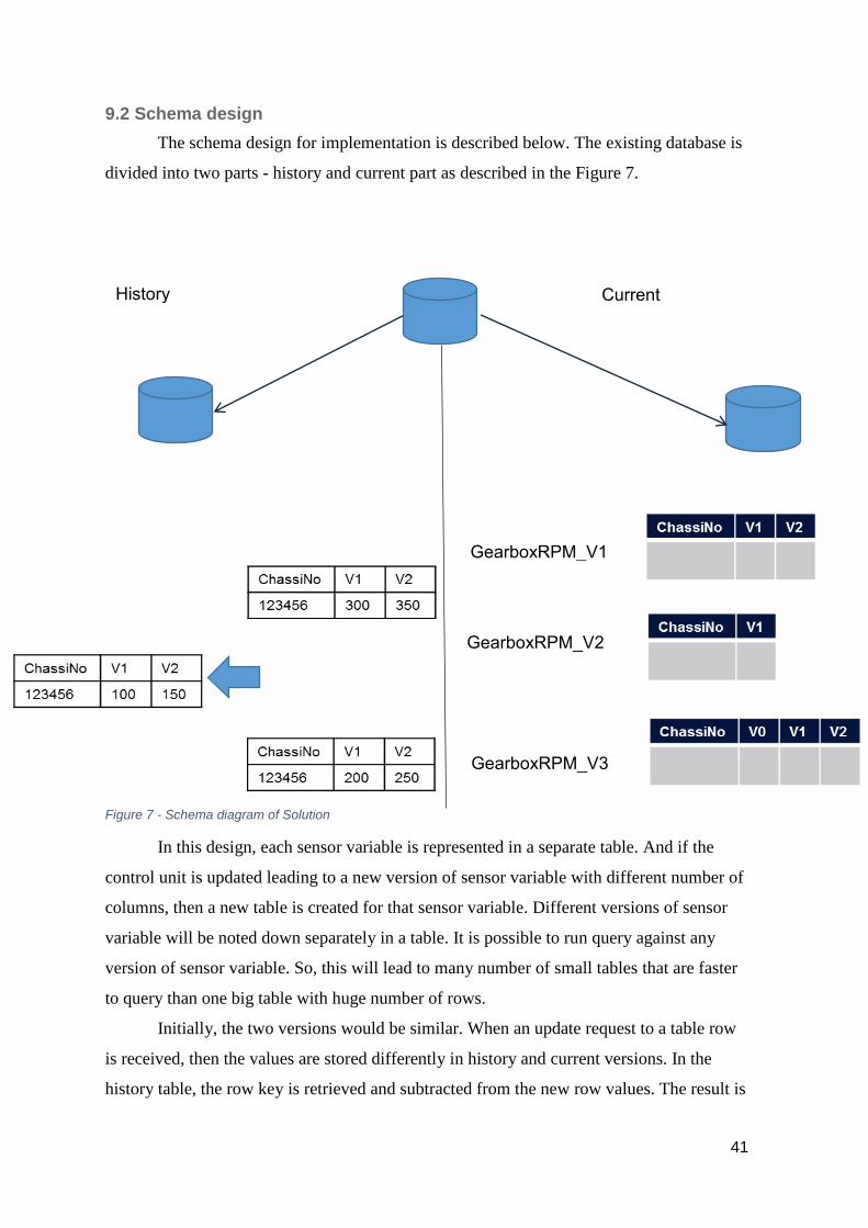
41
9.2 Schema design
The schema design for implementation is described below. The existing database is
divided into two parts - history and current part as described in the Figure 7.
Figure 7 - Schema diagram of Solution
In this design, each sensor variable is represented in a separate table. And if the
control unit is updated leading to a new version of sensor variable with different number of
columns, then a new table is created for that sensor variable. Different versions of sensor
variable will be noted down separately in a table. It is possible to run query against any
version of sensor variable. So, this will lead to many number of small tables that are faster
to query than one big table with huge number of rows.
Initially, the two versions would be similar. When an update request to a table row
is received, then the values are stored differently in history and current versions. In the
history table, the row key is retrieved and subtracted from the new row values. The result is
GearboxRPM_V1
GearboxRPM_V2
GearboxRPM_V3
History Current

42
stored in each of the columns. This is because the values from sensors are accumulated
values. In the current version the new row will replace the existing row for that row key.
This design has the advantage of storing both historic value and latest value of a
sensor variable. The logic behind this design was to allow quick updates to the database
without affecting the ability to run ad-hoc queries or business intelligence queries. Updates
will always be performed against the current version of database and data analytics over the
entire set of values will be performed against the history database.
9.3 MySQL Cluster implementation
Four nodes were used for the practical implementation. MySQL Cluster was
implemented with two data nodes, two SQL nodes and a node performing overlapping role
of Cluster manager. Data nodes were made multithreaded using ndbmtd type for data nodes
in cluster configuration. Also, many connections were used between application nodes and
data node using connection pool parameter. Installation of MySQL Cluster is described in
Appendix A. The BinApproximation algorithm for median was implemented in UDF.
9.4 HBase design and implementation
In the cluster, Hadoop was first installed. So there was a NameNode, a Secondary
NameNode, 4 DataNodes, a Job Tracker and a Task Tracker. Some nodes performed
overlapping roles since there were only 4 nodes. Once it was installed, HDFS was ready as
a storage for HBase. HBase was then installed with a Zookeeper, HMaster and 4 region
servers. Details of how to install Hadoop and HBase are described in Appendix C. Same
schema design was used in HBase as described above. So, we used Apache Sqoop to
import data in to HBase. BinApproximation algorithm was implemented in a MapReduce
program.
9.5 Tests
Tests were conducted in a cluster of 2 nodes which were virtualized into four nodes.
ChassiNo V0 V1 V2… V399
Table 5 – Table to illustrate test run
The above table represents a sample table to illustrate median computation
performed in the database products. A median computation comprised of calculating
median over all the rows of table for each of the columns. In the above case, a median

43
computation was a calculation of median of all 400 columns - median (V0), median
(V1)…median (V399). There were 90,000 rows in the table that was chosen for running
performance tests and it was the one with largest number of rows and columns. This was
because the schema changes introduced many number of small tables corresponding to
sensor variables.
10. Results
The results of running median computation is represented figuratively below in bar charts.
Figure 8 - Total number of median computations for HBase and MySQL Cluster.
BinApproximation algorithm was run in MySQL Cluster and HBase in rounds. The
number of computation was measured by taking an average of values from 10 rounds of
execution where each round was of 30 minutes.
In HBase, sequential execution of MapReduce jobs for this algorithms was run by starting
jobs in sequence after previous job’s completion. Above graph states that there were 22
computations on an average for a round of median computation. Parallel execution of
MapReduce jobs was implemented by submitting multiple jobs and executing them in
parallel. Above graph states that there were 77 median computations on an average for a
round of median computation.
In MySQL Cluster, the algorithm was implemented in UDF. Parallel execution was
implemented by running 10 threads of median computations. Sequential execution was
implemented by running median computations one after another in a single thread.
22
344
77
361
0
50
100
150
200
250
300
350
400
HBase MySQL Cluster
Nu
mb
er
of
Me
dia
n c
alcu
lati
on
s
Total number of Computations
Sequential
Parallel

44
Figure 9 - Execution time of Median Algorithm
Above graph shows execution time of median algorithm in HBase and MySQL
Cluster. This test was run in parallel setting as it fared well as shown in previous graph. It
shows minimum and maximum execution time of median computation over 10 rounds. X
axis denotes execution time in seconds. In this measurement, outliers are eliminated to
produce an approximate comparison. Outliers are execution time measurements which are
extremely high or low and can occur due to external factors such as network load, issues of
virtualization, etc. In HBase the minimum execution time was around 100s and maximum
execution time was around 360s, whereas in MySQL Cluster the minimum execution time
was around 6s and maximum execution time was around 110s.
11. Discussion
In the first graph, it can be seen that the Parallel execution of a MapReduce job was
250% faster than sequential execution of median algorithm in HBase. In case of sequential
execution, jobs were run one after another after each job’s completion. Though map and
reduce tasks were run in parallel, the cluster was not fully utilized. This can be seen by
monitoring the cluster while sequential execution is carried out. However, HBase is
capable of handling execution of multiple jobs in parallel. This is clearly evident in parallel
execution which is 2 times faster than sequential run in the same configuration. So
experimentation was performed with executing several jobs in parallel. Number of jobs that
can be run in cluster in parallel is limited by the cluster size, log files memory and heap
size configuration.
100.831
6.002
363.074
116.763
0
50
100
150
200
250
300
350
400
HBase MySQL Cluster
Exec
uti
on
tim
e in
Sec
on
ds
Execution Time of Median Algorithm
min
max
45
MySQL Cluster had similar execution time for parallel or sequential execution of
median algorithm. In parallel execution multiple threads were run and median computation
is performed. However, the execution time of a single computation took very less time
(around 6s). This is because UDFs are quite powerful and extremely fast since they access
database data structures directly. Thus there is negligible difference in execution time of
median computation between parallel and sequential setting.
MySQL Cluster gave real time performance for median computation. Number of
median computations for a table in MySQL Cluster was more than 5 times faster than that
of same execution in HBase. This can be clearly understood by comparing the execution
time as shown in graph 2.
12. Conclusion
In this thesis, the sensor data analysis project at Scania was studied and analyzed.
Challenges with the existing system was analyzed and future requirements identified. Ideal
properties of a perfect solution for this problem was defined. NoSQL and NewSQL
products were compared against the defined properties. Two interesting products were
chosen, one from each category for practical implementation.
Data analytics over humongous data sets seem possible only by using distributed
computation framework like MapReduce in HBase. Here, MapReduce jobs are submitted
as batch jobs and is capable of running analytics over entire data set and provide high
throughput. It is however not suitable for providing realtime performance. There are tools
to provide realtime data analytics. Storm is an open source distributed system for realtime
computation and data analytics. Typical use case is to do analysis over unbounded streams
in realtime. [14] In the sensor data analysis project, sensor data updates are not very
frequent and does not fit into streaming data category. So, batch processing of ad-hoc
analyses is sufficient. Hence, HBase is more suitable and can be scaled by adding
additional nodes (horizontal scalability).
MySQL Cluster provides realtime performance for ad-hoc analysis since it uses in-
memory storage setting for storing data. It is also capable of handling high volume of
concurrent reads and writes. It provides good performance for large volume of online
transactions. However, it does not provide a parallel programming framework like
MapReduce to implement distributed algorithm. This is still possible using UDFs and
NoSQL APIs. They are quite powerful since they directly access data structures of database

46
as key value pairs. However, they can crash the system if not properly designed and require
special skills. It is not as simple and easy as MapReduce framework.
Performance comparison of the products was done using quantitative comparison
method. Results show that in this setting MySQL Cluster performed better than HBase.
However, this result has to be taken with a pinch of salt and should not be taken as the sole
factor in making a decision. HBase is designed for specific purpose and its merits are
discussed. Similarly MySQL Cluster has its own purpose and merits. It is up to the project
to weigh these factors while choosing between these two distributed database products or a
combination of products for future implementation.
13. Future Work
In this paper, a general exploratory study was performed on distributed databases
available in the market and comparison was performed focusing on the requirements of
Scania’s sensor data analysis project. It was not intended as a comprehensive study of all
interesting products due to time and resource constraints. However, the following areas
have to be investigated further before implementing a database product for Sensor data
analysis project:
Business Intelligence products such as Pentaho can be installed and
integrated with HBase and MySQL Cluster. After integration, real world
queries and ad-hoc analysis should be performed using BI product to
measure performance.
Optimization strategies can be explored for both the products to increase
performance. There are lot of cluster configuration parameters which can be
tuned for good performance. Also, there are application level optimizations
specific to database product which can be studied further.
MySQL Cluster is studied with in-memory storage setting. It can be studied
with local storage setting using SSD disks and enterprise flash drives.
Security was not taken as a criteria while studying different products. This
was because it is a huge field of study in itself. So, security features and
vulnerabilities of chosen products can be investigated further.

47
14. Appendix
A. MySQL Cluster
A.1 Installation
Installation of MySQL Cluster is carried out as per the official documentation [39].
Latest software is downloaded from product downloads page
(http://dev.mysql.com/downloads/cluster/). Generally available edition is the community
edition which developers can use and test the product. It has full features of the product
except that there is no user-friendly cluster manager. The steps are listed below.
1. Latest version tar ball is extracted and a link is created using following commands.
tar xvf mysql-cluster-gpl-7.3.2-linux-glibc2.5-x86_64.tar.gz
ln -s mysql-cluster-advanced-7.2.4-linux2.6-x86_64 mysqlc
2. Following folder and directory structure is created.
mkdir my_cluster my_cluster/ndb_data my_cluster/mysqld_data
my_cluster/conf
3. Two configuration files are created in the conf folder.
my.cnf
[mysqld]
Ndbcluster
Datadir=/home/user/my_cluster/mysqld_data
Basedir=/home/user/mysqlc
Port=5000
ndb-connectstring=$CLUSTER_MGT_NODE:$PORT
ndb-cluster-connection-pool=4
bulk_insert_buffer_size=1024M
max_allowed_packet=1024M
query_cache_size=0
config.ini
[ndb_mgmd]
#Cluster Management node configuration
Hostname=cluster_mgr_node
Datadir=$CLUSTER_HOME/my_cluster/ndb_data
Nodeid=1

48
[ndbd default]
NoOfReplicas=2
MaxNoOfAttributes=10000
DataMemory=4G
IndexMemory=1G
MaxNoOfExecutionThreads=8
[ndbd]
#This is configuration specific to data node 1
Hostname=data_node_1
Datadir=$MYSQL_HOME/data_node_1/my_cluster/ndb_data
[ndbd]
#This is configuration specific to data node 2
Hostname=data_node_2
Datadir=$MYSQL_HOME/data_node_2/my_cluster/ndb_data
[mysqld]
#This is configuration specific to sql node 1
Hostname=sql_node_1
[api]
Hostname=sql_node_1
[api]
Hostname=sql_node_1
[api]
Hostname=sql_node_1
[mysqld]
#This is configuration specific to sql node 2
Hostname=sql_node_2
[api]
Hostname=sql_node_2
[api]
Hostname=sql_node_2
[api]
Hostname=sql_node_2
4. Steps 1-3 are followed for Cluster Management Node. Steps 1 and 2 are followed in
SQL Server nodes and data nodes.

49
5. In SQL Server nodes, MySQL Server is installed using following commands
cd mysqlc
scripts/mysql_install_db --no-defaults –
datadir=$MYSQL_HOME/my_cluster/mysqld_data
Now, the system is installed and ready to be started. It has to be started in the
following order: cluster management node, data nodes and MySQL Servers.
Cluster Manager is started using following command,
$HOME/mysqlc/bin/ndb_mgmd -f conf/config.ini --initial --
configdir=$HOME/my_cluster/conf/
Data nodes are started using following command,
$HOME/mysqlc/bin/ndbd -c $CLUSTER_MGT_NODE:$PORT
Above nodes should be started before starting MySQL Server and hence their status
is checked using following command in management node,
$HOME/mysqlc/bin/ndb_mgm -e show
Then the MySQL Servers are started
$HOME/mysqlc/bin/mysqld --defaults-file=conf/my.cnf &
A.2 Administration
To connect to the MySQL Server, following command is used.
$HOME/mysqlc/bin/mysql -h $SQL_Server -P 5000 -u root
To shut down the MySQL Server following command is used.
$HOME/mysqlc/bin/mysqladmin -u root -h $SQL_Server -P 5000 shutdown
To shut down the MySQL Cluster following command is used.
$HOME/mysqlc/bin/ndb_mgm -e shutdown
To connect to the MySQL Servers using Java program, a load balanced connect string
should be used -
jdbc:mysql:loadbalance://server1_hostname,server2_hostname:$PORT/$Database

50
B. HBase
B.1 Installation
To install HBase, a distributed file system is required. So, Hadoop is first installed.
HBase only supports some versions of Hadoop. Version matrix of supported versions can
be found in the official documentation. [40] It also provides detailed instructions for
installation of HBase.
Hadoop tar ball is downloaded from official site -
http://hadoop.apache.org/releases.html#Download
1. The tar ball is extracted using tar command.
tar xvf hadoop-1.2.1.tar.gz
2. It is essential to change default value of parameter JAVA_HOME to that of
local java installation in the configuration file Hadoop/conf/Hadoop-env.sh
3. RSA key is created to be used by Hadoop when it accesses localhost or
other nodes in cluster using SSH.
SSH-keygen –t rsa –P “”
cat ~/.ssh/id_rsa.pub >> ~/.ssh/authorized_keys
4. Above steps are repeated for each of nodes in the cluster.
5. Configuration files are modified as below.
Core-site.xml
<configuration>
<property>
<name>fs.default.name</name>
<value>hdfs://$NAME_NODE:$PORT</value>
</property>
</configuration>
Mapred-site.xml
<configuration>
<property>
<name>mapred.job.tracker</name>
<value>$JOB_TRACKER:$JOBTRACKER_PORT</value>
</property>
</configuration>
Hdfs-site.xml

51
<configuration>
<property>
<name> dfs.name.dir</name>
<value>$HADOOP_HOME/name_dir</value>
</property>
<property>
<name> dfs.data.dir</name>
<value>$HADOOP_HOME/data_dir</value>
</property>
<property>
<name> dfs.replication</name>
<value>2</value>
</property>
</configuration>
6. The configuration files are synchronized across all nodes in cluster using
rsync command. Hadoop file system is formatted using following command
./bin/hadoop namenode -format
7. Now, Hadoop is installed and ready to be started.
./bin/start-all.sh
Once Hadoop is installed, HBase can be installed. HBase version is downloaded from
following page - http://apache.mirror3.ip-only.net/hbase/hbase-0.95.2/
1. Default limits on number of file descriptors and procedures is not sufficient
for HBase. These limits are changed in /etc/security/limits.conf using
following commands,
hadoop - nofile 32768
hadoop soft/hard nproc 32000
2. The tar ball is extracted in all nodes of the cluster. Following changes to
configuration file is made.
hbase-site.xml
<configuration>
<property>
<name>hbase.rootdir</name>
<value>hdfs://$NAME_NODE:$PORT/hbase</value>

52
</property>
<property>
<name>hbase.cluster.distributed</name>
<value>true</value>
</property>
<property>
<name>dfs.datanode.max.xceivers</name>
<value>4096</value>
</property>
<property>
<name>hbase.zookeeper.property.dataDir</name>
<value>zookeeper_data_dir</value>
</property>
<property>
<name>hbase.zookeeper.property.clientPort</name>
<value>zookeeper_port</value>
</property>
<property>
<name>hbase.zookeeper.quorum</name>
<value>$zookeeper</value>
</property>
</configuration>
Hbase-env.sh
export HBASE_MANAGES_ZK=true
export HBASE_HEAPSIZE=4096
export JAVA_HOME=/usr/java/latest
region servers
#host name for each region server
3. Location of hadoop/conf directory is added to HBASE_CLASSPATH in
hbase-env.sh
4. HBase installation is tested using start command.
bin/start-hbase.sh

53
B.2 Administration
Hadoop administration commands follows a generic pattern [35]
bin/hadoop [COMMAND] [GENERIC_OPTIONS] [COMMAND_OPTIONS]
Command can be one of the following – dfsadmin, fs, fsck, jar, and job
1. Dfsadmin – used for running DFS administrative client. Detailed options are shown
in documentation. [41]
2. Fs – used for displaying/manipulating file system.
3. Fsck – used to run file system checking utility.
4. Jar – used for running user code or map reduce jobs. Input and output location can
be specified along with formats.
5. Job – used to track and administer map reduce jobs.
6. There are commands to run data node, job tracker node, task tracker node,
secondary namenode, and MapReduce client.
To print information about data nodes, use following command bin/hadoop dfsadmin -
report
HBase provides a JRuby shell which can be invoked using,
bin/hbase shell
There are many shell commands to create database, table, columns, columnfamily, etc.
Comprehensive list of shell commands can be found in hbase wiki. [42]
There are also many tools and utilities provided for HBase and are listed in documentation
page. [43]
54
References
[1] ‘Scania AB - Wikipedia, the free encyclopedia’. [Online]. Available:
http://en.wikipedia.org/wiki/Scania_AB. [Accessed: 22-September-2013].
[2] ‘Scania in Brief - scania.com’. [Online]. Available: http://www.scania.com/scania-
group/scania-in-brief/index.aspx. [Accessed: 22-September-2013].
[3] ‘What is Data Aggregation? - Definition from Techopedia’. [Online]. Available:
http://www.techopedia.com/definition/14647/data-aggregation. [Accessed: 26-
September-2013].
[4] ‘Gartner IT Glossary - Big Data’. [Online]. Available: http://www.gartner.com/it-
glossary/big-data/. [Accessed: 26-September-2013].
[5] ‘NewSQL -- The New Way to Handle Big Data - LINUX For You’. [Online].
Available: http://www.linuxforu.com/2012/01/newsql-handle-big-data/. [Accessed: 23-
September-2013].
[6] W. H. Inmon, ‘Building the data warehouse: getting started’, Disponível por www em
http://impactline. net/% C0% DA% B7% E1% C3% B7% BA% CE% B9%
B0/OLAPDW/ttbuild (Inmon). pdf, 2000, Available at http://inmoncif.com/inmoncif-
old/www/library/whiteprs/ttbuild.pdf.
[7] L. Bonnet, A. Laurent, M. Sala, B. Laurent, and N. Sicard, ‘Reduce, You Say: What
NoSQL Can Do for Data Aggregation and BI in Large Repositories’, 2011, pp. 483–
488, DOI:10.1109/DEXA.2011.71, Available at
http://ieeexplore.ieee.org/lpdocs/epic03/wrapper.htm?arnumber=6059864.
[8] ‘LESSON - Data Aggregation—Seven Key Criteria to an Effective Aggregation
Solution -- TDWI -The Data Warehousing Institute’. [Online]. Available:
http://tdwi.org/articles/2005/04/26/data-aggregationseven-key-criteria-to-an-effective-
aggregation-solution.aspx. [Accessed: 26-September-2013].
[9] ‘Big Data Definition from PC Magazine Encyclopedia’. [Online]. Available:
http://www.pcmag.com/encyclopedia/term/62849/big-data. [Accessed: 26-September-
2013].
[10] ‘NOSQL Databases’. [Online]. Available: http://nosql-database.org/. [Accessed:
23-September-2013].
[11] ‘Data Warehouses, Schemas and Decision Support Basics by Dan Power -
BeyeNETWORK’. [Online]. Available: http://www.b-eye-network.com/view/8451.
[Accessed: 26-September-2013].
[12] ‘A Vendor-independent Comparison of NoSQL Databases: Cassandra, HBase,
MongoDB, Riak - Software Product Development Services | Altoros’. [Online].
Available: http://www.altoros.com/nosql-research. [Accessed: 26-September-2013].
[13] W. Munir, ‘Optimization of Data Warehouse Design and Architecture’, KTH,
2011, Available at http://kth.diva-portal.org/smash/record.jsf?pid=diva2:432740.
[14] ‘Storm, distributed and fault-tolerant realtime computation’. [Online]. Available:
http://storm-project.net/. [Accessed: 14-September-2013].
[15] Baron Schwartz, Peter Zaitsev, Vadim Tkachenko, High Performance MySQL, 3rd
ed. O’Reilly Media, Inc., 2012, ISBN: 978-1449314286.
[16] Shashank Tiwari, Professional NoSQL. Wiley / Wrox, 2011, ISBN: 978-
0470942246.
[17] ‘Agile Development and Experience Design | ThoughtWorks’. [Online]. Available:
http://www.thoughtworks.com/insights/articles/nosql-comparison. [Accessed: 26-
September-2013].
[18] G. DeCandia, D. Hastorun, M. Jampani, G. Kakulapati, A. Lakshman, A. Pilchin,
S. Sivasubramanian, P. Vosshall, and W. Vogels, ‘Dynamo: amazon’s highly available

55
key-value store’, in ACM Symposium on Operating Systems Principles: Proceedings of
twenty-first ACM SIGOPS symposium on Operating systems principles, 2007, vol. 14,
pp. 205–220, Available at http://www.read.seas.harvard.edu/~kohler/class/cs239-
w08/decandia07dynamo.pdf.
[19] ‘In-Memory Data Grid - Hazelcast’. [Online]. Available:
http://www.hazelcast.com/whatishazelcast.jsp. [Accessed: 26-September-2013].
[20] ‘Infinispan - Open Source Data Grids - JBoss Community’. [Online]. Available:
https://www.jboss.org/infinispan. [Accessed: 26-September-2013].
[21] ‘XAP In-Memory Computing software platform for Real Time Event Processing |
GigaSpaces’. [Online]. Available: http://www.gigaspaces.com/xap-in-memory-
computing-event-processing/Meet-XAP. [Accessed: 26-September-2013].
[22] ‘Spring Data Gemfire’. [Online]. Available: http://projects.spring.io/spring-data-
gemfire/. [Accessed: 26-September-2013].
[23] ScaleBase, ‘Choosing a Next Gen Database: the New World Order of NoSQL,
NewSQL,...’, 25-March-2013, Available at
http://www.slideshare.net/ScaleBase/choosing-a-next-gen-database-the-new-world-
order-of-no-sql-newsql-and-mysql.
[24] ‘NuoDB | NewSQL | Scale-out | Cloud Database | Documents’. [Online]. Available:
http://www.nuodb.com/resources/documents/. [Accessed: 16-September-2013].
[25] ‘What Exactly Is Database as a Service? | Database as a Service’. [Online].
Available: http://dbaas.wordpress.com/2008/05/14/what-exactly-is-database-as-a-
service/. [Accessed: 18-September-2013].
[26] ‘How the Database Cloud provides a scaleable and reliable solution | StormDB’.
[Online]. Available: http://www.stormdb.com/sql-database-fabric. [Accessed: 18-
September-2013].
[27] ‘ThinkMind(TM) Digital Library’. [Online]. Available:
http://www.thinkmind.org/index.php?view=article&articleid=cloud_computing_2011_
6_30_20083. [Accessed: 26-September-2013].
[28] ‘PolyglotPersistence’. [Online]. Available:
http://www.martinfowler.com/bliki/PolyglotPersistence.html. [Accessed: 23-
September-2013].
[29] Tom White, Hadoop: The Definitive Guide, 3rd ed. O’Reilly Media, Inc., ISBN:
978-1449311520.
[30] ‘HDFS Architecture Guide’. [Online]. Available:
http://hadoop.apache.org/docs/r1.0.4/hdfs_design.html. [Accessed: 23-September-
2013].
[31] Lars George, HBase: The Definitive Guide, 1st ed. O’Reilly Media, Inc., 2011,
ISBN: 978-1-4493-9610-7.
[32] ‘9.6. RegionServer’. [Online]. Available:
http://hbase.apache.org/book/regionserver.arch.html. [Accessed: 28-August-2013].
[33] Herodotos Herodotou, ‘Hadoop Performance Models’, Computer Science
Department Duke University Abstract, no. Technical Report, CS-2011–05, Available at
http://www.cs.duke.edu/starfish/files/hadoop-models.pdf.
[34] ‘MySQL :: MySQL 5.5 Reference Manual :: 17.3.2.6 Defining MySQL Cluster
Data Nodes’. [Online]. Available: http://dev.mysql.com/doc/refman/5.5/en/mysql-
cluster-ndbd-definition.html#ndbparam-ndbmtd-maxnoofexecutionthreads. [Accessed:
03-September-2013].
[35] ‘Optimizing the Performance Of MySQL Cluster’. [Online]. Available:
http://www.agileload.com/agileload/blog/2013/03/11/optimizing-the-performance-of-
mysql-cluster. [Accessed: 23-September-2013].

56
[36] ‘MySQL :: MySQL 5.6 Reference Manual :: 17.6.11 MySQL Cluster Replication
Conflict Resolution’. [Online]. Available:
http://dev.mysql.com/doc/refman/5.6/en/mysql-cluster-replication-conflict-
resolution.html. [Accessed: 26-September-2013].
[37] MySQL Innovation Day: MySQL Cluster - What’s New, What’s Coming. 2012,
Available at
https://www.youtube.com/watch?v=pbXrciXrRdw&feature=youtube_gdata_player.
[38] R. J. Tibshirani, ‘Fast computation of the median by successive binning’, arXiv
preprint arXiv:0806.3301, 2008, Available at http://arxiv.org/abs/0806.3301.
[39] ‘MySQL :: MySQL 5.5 Reference Manual :: 17.2 MySQL Cluster Installation and
Upgrades’. [Online]. Available: http://dev.mysql.com/doc/refman/5.5/en/mysql-cluster-
installation.html. [Accessed: 08-September-2013].
[40] ‘The Apache HBaseTM Reference Guide’. [Online]. Available:
http://hbase.apache.org/book.html. [Accessed: 21-September-2013].
[41] ‘Commands Guide’. [Online]. Available:
http://hadoop.apache.org/docs/stable/commands_manual.html. [Accessed: 21-
September-2013].
[42] ‘Hbase/Shell - Hadoop Wiki’. [Online]. Available:
http://wiki.apache.org/hadoop/Hbase/Shell. [Accessed: 21-September-2013].
[43] ‘Chapter 15. Apache HBase Operational Management’. [Online]. Available:
http://hbase.apache.org/book/ops_mgt.html. [Accessed: 21-September-2013].