A Study of One Dimensional Population Balance

Modeling Techniques for Crystallization Processes

Pranav Anant Mashankar

External Supervisor: Prof. Johannes Khinast and Georg Scharrer

Research Center Pharmaceutical Center (RCPE)

Inffeldgasse 13, Graz, Austria 8010

Internal Supervisor: Prof. Rohit Ramachandran

Rutgers-The State University of New Jersey

98 Brett Road, Piscataway, NJ-08854

2

CONTENTS

ACKNOWLEDGEMENTS ......................................................................................................................... 3

CRYSTALS: AN INTRODUCTION............................................................................................................... 4

PHYSICAL AND CHEMICAL PROPERTIES OF CRYSTALS .................................................................................. 8

NUCLEATION .................................................................................................................................... 13

CRYSTAL GROWTH ............................................................................................................................ 22

POPULATION BALANCE EQUATIONS: AN INTRODUCTION .......................................................................... 26

THE ONE DIMENSIONAL POPULATION BALANCE EQUATION ...................................................................... 28

BIRTH AND DEATH FUNCTIONS ............................................................................................................ 33

SOLUTION METHODS FOR POPULATION BALANCE EQUATIONS .................................................................. 44

CASE STUDY - ONE DIMENSIONAL POPULATION BALANCE MODEL OF A BATCH COOLING CRYSTALLIZATION

PROCESS ......................................................................................................................................... 48

CONCLUSION ................................................................................................................................... 56

BIBLIOGRAPHY.................................................................................................................................. 57

3

ACKNOWLEDGEMENTS

I am deeply indebted to the Marshall Plan Foundation for affording me the unique

opportunity to work at RCPE in Graz University of Technology, Austria. This has

been an extremely enriching experience through which I have got a chance to

learn from people with vast experience in the pharmaceutical industry.

I thank Dr Johannes Khinast and Mr Georg Scharrer for their invaluable guidance

and support during my time in Graz. I also thank Kathrin Manninger for

wholeheartedly assisting me with a wide spectrum of issues ranging from the

Marshall Plan Scholarship application to accomodation in Graz. It was only

because of Kathrin’s prompt help that I was able to singlemindedly focus on

academics during my 3 months at TU Graz. I am also extremely grateful to my

colleagues at TU Graz for their support, especially Maximilian Besenhardt at

RCPE for his invaluable guidance.

I thank Dr Rohit Ramachandran, my adviser at Rutgers University for

recommending my name for this prestigious scholarship program. Dr

Ramachandran has been a constant source of encouragement and guidance

during my research at Rutgers University. I thank Dr Yee Chiew at Rutgers

University for his guidance during the application process for the Marshall Plan

Scholarship. Lastly I thank my family and my countless friends and classmates

who have been a continual source of encouragement and support.

4

CRYSTALS: AN INTRODUCTION

All solid matter may be classified as either amorphous or crystalline. The

crystalline state differs from the amorphous state in the regular arrangement of

its constituent molecules. Crystals are anisotropic, that is, their mechanical,

electrical, magnetic and optical properties vary according to the direction in which

they are measured. Crystals belonging to the cubical system are a notable

exception.

A crystal consists of a lattice of molecules, atoms or ions whose locations in the

lattice are unique to each substance. This regularity in internal structure results in

a characteristic crystal shape for each crystalline substance.

Many of the geometric shapes that appear in the crystalline state are readily

recognized as being symmetrical and this fact can be used as a means of crystal

classification. The three elements of symmetry considered are,

1. Symmetry about a point,

2. Symmetry about a line,

3. Symmetry about a plane

A crystal possesses a centre of symmetry when every point on the surface of the

crystal has an identical point on the opposite side of the centre, equidistant from

it. One such example is a cube.

A crystal possesses an axis of symmetry if, when the crystal is rotated once

around the said axis (i.e., 360⁰), it appears to have reached its original position

more than once. If a crystal has rotated through 180⁰ before appearing to reach

its original position, the axis is one of two fold symmetry(Mullin). If it has rotated

through 120⁰, 90⁰ or 60⁰ the axes are of threefold symmetry (triad axis), fourfold

5

symmetry (tetrad axis) and sixfold symmetry (hexad axis), respectively. A cube

has 13 axes of symmetry, 6 diad axes through opposite edges, 4 triad axes

through opposite corners and 3 tetrad axes through opposite faces(Mullin).

A plane of symmetry bisects an object such that one half becomes a mirror

image of the other half in the given plane. A cube has 9 planes of symmetry, 3

rectangular planes each parallel to two faces, and 6 diagonal planes passing

through opposite edges.

Crystal systems: crystals may be grouped into 7 systems(Mullin). These are

1. Regular,

2. Tetragonal,

3. Orthorhombic

4. Monoclinic,

5. Triclinic,

6. Trigonal and

7. Hexagonal

The first six of these systems can be described with reference to three axes, x, y

and z. The angle between the y and z axes is denoted by α, that between x and z

by β and that between x and y by γ. Four axes are required to describe the

hexagonal system. The z axis is vertical and perpendicular to the other three

axes (x, y and u), which are coplanar and inclined at 60⁰ to one another.

A brief comparative description of the seven systems is given in the following

table(Mullin).

6

System Other names Angles

between axes

Length of

axes

Examples

Regular Cubic

Octahedral

Isometric

Tesseral

α=β=γ=90⁰ x=y=z Sodium

chloride

Potassium

chloride

Alums

Diamond

Tetragonal Pyramidal

Quadratic

α=β=γ=90⁰ x=y≠z Rutile

Zircon

Nickel

sulphate.7H2O

Orthorhombic Rhombic

Prismatic

Isoclinic

Trimetric

α=β=γ=90⁰ x≠y≠ z Potassium

permanganate

Silver nitrate

Iodine

α-Sulphur

Monoclinic Monosymmetric

Clinorhombic

Oblique

α=β=90⁰

γ≠90⁰

x≠y≠ z Potassium

chlorate

Sucrose

Oxalic acid

β-Sulphur

Triclinic Anorthic

Asymmetrical

α≠β≠γ≠90⁰ x≠y≠ z Potassium

dichromate

Copper

sulphate.5H2O

Trigonal Rhombohedral α=β=γ≠90⁰ x=y=z Sodium nitrate

Ruby

Sapphire

7

Hexagonal None Z axis is

perpendicular

to the x, y and

u axes, which

are inclined at

60⁰

X=y=u≠z Silver iodide

Graphite

Water(ice)

Potassium

nitrate

Bonding in crystals: Crystalline solids may be classified into four main types

according to their method of bonding viz. ionic, covalent, molecular and

metallic(Mullin).

Ionic crystals are composed of charged ions held in place in the lattice by

electrostatic forces, and separated from the oppositely charged ions by regions

of negligible electron density.

In covalent crystals the constituent atoms do not carry effective charges; they are

connected by a framework of covalent bonds.

Molecular crystals are composed of discrete molecules held together by weak

attractive forces.

Metallic crystals consist of ordered arrays of identical cations. The constituent

atoms share their outer electrons as in covalent bonds, but these are so loosely

held that they are free to move through the crystal lattice and give metallic

properties to the bond.

Polymorphism and Racemism: crystals may exist as isomorphs and polymorphs.

Isomorphs are those crystals that crystallize in almost identical forms and are

chemically similar. Polymorphs on the other hand are chemically identically

crystals that crystallize in different forms.

8

PHYSICAL AND CHEMICAL PROPERTIES OF CRYSTALS

Growth and nucleation kinetics of crystals depend on the deformation of the

crystal lattice. The degree of deformation is a function of the shear modulus,

Young’s modulus, the Poisson ratio and the fracture resistance. An isotropic

material has two elasticity constants, the shear modulus and the Poisson’s ratio

from which all possible constants can be calculated. Anisotropic materials on the

other hand may have between 3 (for the cubic system) and 21 (for the triclinic

system) elastic constants depending on the symmetry. Assuming that impacts on

a crystal are distributed statistically in all axial directions, the effective (isotropic)

elastic properties can be estimated from the constants. The Poisson ratio is give

as

νc = E/2μ – 1

where E is the Young’s modulus and μ is the shear modulus.

The attrition of crystals due to mechanical impact depends on the brittleness of

the material. This brittleness can be described by a ration of the Young’s

modulus E and the hardness H. materials with a high E/H ratio (>180) are more

ductile(Mersmann).

Surface tension of crystals: The interfacial tension ϒCL between the solid phase

and the surrounding mother liquor is of importance for primary nucleation and for

integration limited growth(Mersmann). In both cases, the kinetics is limited by a

thermodynamic balance; the free enthalpy, which is gained proportional to the

9

crystallized volume, must extend the free enthalpy necessary to build the new

surface(Mersmann). In principle, ϒCL is comparable to the surface tension of a

liquid phase in equilibrium with its vapor. However, because of restricted mobility

of the molecules in the solid phase, the surface is not usually at minimum free

energy. Structural damage that the crystal has undergone will contribute to

surface stress, τCL. The total energy per unit area is given by(AW Adamson)

τCL = ϒCL + A(δ τCL/δA)

Supersaturation: Crystallization processes are best represented by enthalpy-

concentration diagrams. The number of collisions of elementary units like atoms

ions and molecules with those in the fluid phase or at the phase interface of the

crystalline phase depends on the number of units per unit volume of the fluid

phase(Mersmann):

=

=

A saturated fluid having concentration C* is in thermodynamic equilibrium with the

solid phase at the relevant temperature. If the solution is liquid, the saturation

concentration often depends strongly on the temperature but only slightly on the

10

pressure(Mersmann). If a fluid phase has more units than C*Na, it is said to be

supersaturated. Crystallization processes can take place only in supersaturated

phases, and the rate of crystallization is often determined by the degree of

supersaturation. Supersaturation is expressed either as a difference in

concentration(Mersmann)

∆C = C – C*

Or as relative supersaturation(Mersmann),

S = C/C*

The fundamental driving force for crystallization is the difference between the

chemical potential of a given substance in the transferring and the transferred

state, i.e., in solution (state 1) and the crystal (state 2). For an unsolvated solute

crystallizing from a binary solution, this may be written as(Mersmann)

∆μ = μ1 – μ2

The chemical potential is defined in terms of the standard chemical potential μ0

and the activity ‘a’ by(Mersmann)

μ = μ0 + RTlna

11

the fundamental driving force for crystallization may therefore be expressed as

(Mersmann)

∆ μ/RT = ln(a/a*) = lnS’

Where a* is the activity for a saturated solution, S’ the activity supersaturation, R

the gas constant, and T the absolute temperature, i.e.,

S’ = e∆μ/RT

For electrolytic solutions, use of mean ionic activity a+ is more appropriate. This is

defined by(Mersmann)

a = aν+-

where ν is the number of moles of positive and negative ions in one mole of

solute. Therefore

∆ μ/RT = νlnSa

12

Where

Sa = a+-/a+-*

Solubility: The saturation concentration of a substance in a solvent is obtained

experimentally by determining the maximum amount that is soluble at a given

temperature. Solubility often increases with temperature, but there are also other

systems in which the saturation concentration remains approximately constant or

decreases with an increase in temperature. The solubility curve for hydrates has

a kink where the number of solvent molecules per molecule of dissolved

substance changes(Mersmann).

13

NUCLEATION

Nucleation requires supersaturation, which is obtained usually by a change in

temperature (cooling in case of a positive gradient of the solubility curve and

heating in case of a negative gradient), by removing the solvent, or by adding a

drowning out agent or reaction partners(Mersmann). The system then attempts

to attain thermodynamic equilibrium through nucleation. If the solution contains

neither solid foreign particles nor crystals of its own type, nuclei are formed only

through homogeneous nucleation. If foreign particles are present then nuclei are

formed through heterogeneous nucleation. Both homogeneous nucleation and

heterogeneous nucleation are classified as primary nucleation. This primary

nucleation occurs only when metastable supersaturation is achieved in the

system. However, it has been observed that nuclei occur even at very low

supersaturation levels (less than metastable supersaturation) when solution-own

crystals are present. This type of nucleation is called secondary nucleation. This

may result from contact, shearing action, breakage, abrasion, and needle

fraction(Mersmann).

14

(Mersmann)

Primary Nucleation

Homogeneous nucleation: For the formation of crystal nuclei, the constituent

molecules have to first coagulate, resisting the tendency to redissolve, following

which they have to become oriented in a fixed lattice. Stable nuclei arise from a

sequence of bimolecular additions as follows(Mullin):

A + A ↔ A2

A2 + A ↔ A3

An-1 + A ↔ An (critical cluster)

Nucleation

Primary

Homogeneous

Heterogeneous

Secondary

Contact

Shear

Fracture

Attrition

Needle

15

Further molecular additions to the critical cluster result in nucleation and

subsequent growth of the nucleus(Mullin). Similarly, ions or molecules in a

solution can form short lived clusters. Short chains may be formed initially and

eventually a crystalline lattice is built up. The construction process can only

continue in local regions of very high supersaturation and many sub-nuclei fail to

mature and form nuclei, simply redissolving instead(Mullin). However, if a

nucleus grows beyond a certain critical size, it becomes stable. The structure of

this critical nucleus is not known, and it is too small to observe directly.

The classical theory of nucleation is based on the condensation of a vapor to a

liquid. The free energy changes associated with the process of homogeneous

nucleation are as follows(Mersmann).

The overall excess free energy, ∆G, between a small solid particle of solute

(assumed to be a sphere of radius r for the sake of simplicity) and the solute in

the solution is equal to the sum of the surface free energy, ∆GS, i.e. the excess

free energy between the surface of the particle and the bulk of the particle, and

the volume excess free energy, ∆GV, i.e. the excess free energy between a very

large particle (r = ∞) an the solute in solution. ∆GS is a positive quantity, the

magnitude of which is proportional to r2. In a supersaturated solution ∆GV is a

negative quantity proportional to r3. Thus

∆G = ∆GS + ∆GV

= 4πr2γ + (4/3) πr3∆GV (Mullin)

Where ∆GV is the free energy change of the transformation per unit volume and γ

is the interfacial tension i.e., between the developing crystalline surface and the

supersaturated solution in which it is located. The two terms on the right hand

side of the equation above are of opposite sign and depend differently on r, so

the free energy of formation, ∆G, passes through a maximum, which corresponds

16

to the critical nucleus, rc and for a spherical cluster is calculated by optimizing the

aforementioned equation. Thus,

d∆G/dr = 8πr2∆GV = 0

therefore,

rc = =2γ/∆GV

where ∆GV is a negative quantity. From the above result we get

∆Gcrit = 4πγr2c/3

The behavior of a newly created crystalline lattice structure in a supersaturated

solution depends on its size. It can either grow or dissolve depending on which

process results in a decrease of free energy of the particle. The critical size, rc

therefore represents the minimum size of a stable nucleus(Mullin).

The energy of a fluid system at constant temperature and pressure is constant,

however this does not mean that the energy level is same at all parts of the fluid.

There will be fluctuations in the energy about the constant value, which is to say

that there will be a statistical distribution of energy in the molecules constituting

the system (molecular velocity) and in those supersaturated regions where the

energy rises temporarily to a high value nucleation will be favored(Mullin).

17

The rate of nucleation, J, can be expressed as the Arrhenius reaction velocity

equation commonly used for the rate of a thermally activated process(Mullin):

J = Ae(-∆G/kT)

Where k is the Boltzmann constant.

The basic Gibbs Thomson relationship for a non electrolyte may be written as

lnS = 2γν/kTr (Mullin)

where S is the supersaturation given by S = c/c*, c being the concentration and c*

being the concentration at supersaturation. Ν is the molecular volume. Thus,

∆GV = 2γ/r = kTlnS/ν

Hence,

Gcrit = 16πγ3ν2/3(kTlnS)

Finally,

18

J = Aexp(-(16πγ3ν2)/(3k3T3(lnS)2))

This equation shows that three main variables govern the rate of nucleation,

temperature, T, the degree of supersaturation, S and interfacial tension, γ.

An empirical approach that expresses a relationship between the induction

period, tind (the time interval between mixing two reacting solutions and the

appearance of crystals) and the initial concentration, c of the supersaturated

solution may be expressed as follows (Nielsen)

tind = kc1-p

where k is a constant and p is the number of molecules in a critical nucleus.

Measurement of homogeneous nucleation: In an early attempt to study

nucleation(Vonnegaut) a liquid system was dispersed into a large number of

discrete droplets, exceeding the number of heteronuclei present. A significant

number of droplets were therefore mote-free and could be used or the study of

true homogeneous nucleation.

An expansion cloud chamber was used by Miller Anderson et al (1983) to

measure homogeneous nucleation rate of water over a wide range of

temperature from 230-290K and nucleation rates of 1-1016 drops cm-3s-1. The

comprehensive nature of this data allows for a detailed comparison between

theoretical and experimental work. The expansion chamber technique employs

continuous pressure measurement and an adiabatic pulse of supersaturation to

give the time history of supersaturation and temperature during the nucleation.

19

The resulting drop concentration is determined using photographic

techniques(RC Miller).

Predicting the nucleation rate quantitatively is not a trivial task, and deviations of

several orders of magnitude between theoretical predictions and experimentally

determined nucleation rates are common. Small angle X-ray scattering

experiments have been employed to measure the mean radius, the width of the

distribution function and the particle number density as a function of the initial

mixture composition. Static pressure trace measurement experiments were

conducted to measure the temperature, partial pressure, supersaturation and

characteristic time corresponding to the peak nucleation rates and this data was

combined with that obtained from SAXS experiments to directly quantify

nucleation rate as a function of temperature and supersaturation(D Ghosh).

Heterogeneous nucleation: Even a very small amount of impurities in a solution

may affect the rate of nucleation greatly. However, an impurity may have different

effects on different solutions and may not have an inhibiting effect in all cases; in

fact, it may even act as an accelerator sometimes(Mullin).

It has been observed in many cases that what initially appears to be a case of

homogeneous nucleation has actually been induced in some way(Mullin). In that

sense there is very sparse occurrence of truly homogeneous nucleation. For

example, a supercooled system can be seeded unknowingly by the presence of

atmospheric dust containing active particles i.e., heteronuclei.

The presence of a foreign body surface can induce nucleation at degrees of

supersaturation lower than those required for spontaneous (homogeneous)

nucleation(Mullin). Thus the overall free energy associated with the formation of

a critical nucleus under heterogeneous conditions ∆G’crit, should be less than the

20

corresponding free energy change, ∆Gcrit associated with homogeneous

nucleation. Hence,

∆G’crit = φ∆Gcrit

Where the factor φ is less than 1.

Secondary nucleation

A supersaturated solution nucleates more readily when crystals of the solute are

already present or deliberately added. This type of nucleation is called secondary

nucleation, as opposed to primary nucleation where crystals of the solute are not

present initially(Mullin).

Contact nucleation

It has been observed that even at moderate levels of supersaturation, crystal

contacts readily cause secondary nucleation. In the secondary nucleation of

MgSO4.7H2O crystal-crystal contacts gave up five times as many nuclei as did

crystal-metal rod contacts(NA Clontz).

Crystal agitator contacts may be a cause for secondary nucleation in

crystallizers.

21

Seeding

Seeding of a supersaturated solution with small particles of material to be

crystallized is probably the best method for inducing crystallization. Deliberate

seeding may be used to have some degree of control over the product size and

size distribution. Seed crystals however, need not necessarily consist of the

material being crystallized.

Seed crystal size is considered to be influential in secondary nucleation(RW

Rousseau). There may be several reasons for this. Large seeds generate more

secondary nuclei than do small seeds because of their greater contact

probabilities and collision energies. Very small crystals can follow the streamlines

within the turbulence eddies in vigorously agitated solutions, essentially behaving

as if they were suspended in a stagnant fluid, rarely coming into contact with the

agitator or other crystals(Mersmann).

Unintentional Seeding

Uncontrolled seeding is frequently encountered in the laboratory and in the

industry and it is an uncontrolled event that can cause considerable frustration if

not checked.

22

CRYSTAL GROWTH

Crystal growth occurs as soon as nuclei with radius larger than the critical radius

have been formed. There are many proposed mechanisms for crystal growth.

The surface energy theories are based on the hypothesis that the shape a

growing crystal assumes is such that it has a minimum surface energy. This

approach largely fallen out of favor.

Diffusion theories assume that matter is deposited continuously on the crystal

face at a rate proportional to the difference in concentration between the point of

deposition and the bulk of the solution.

When dealing with crystal growth in an ionizing solute, the following steps can be

distinguished (Mullin)

1. Bulk diffusion of solvated ions through the diffusion boundary layer

2. Bulk diffusion of solvated ions through adsorption layer

3. Surface diffusion of solvated or unsolvated ions

4. Partial or total desolvation of ions

5. Integration of ions into the lattice

6. Counterdiffusion through adsorption layer of water released

7. Counterdiffusion of water through the boundary layer

The slowest of these steps are rate determining(Mersmann).

A crystal surface grow in such a way that units in a supersaturated solution are

first transported by diffusion and convection and then built into the surface of the

crystal by integration or an integration reaction , with the supersaturation, ∆c,

being the driving force.

23

The entire concentration gradient, ∆c = c - c*, is divided into two parts. The first

part, c - cI is responsible for diffusive-convective transport. The second part, cI –

c* is responsible for the integration reaction within the boundary

layer.(Mersmann)

Thus, for growth completely determined by diffusion and convection,

cI – c* << c - cI (Mersmann)

And, when growth is controlled by integration reaction,

cI – c* >> c - cI (Mersmann)

The mass flux density m directed towards the crystal surface is

m = kd(c – cI) = kr(cI – c*)r

herem kd is the mass transfer coefficient, kr is the reaction rate constant and r is

the order of the integration reaction(Mersmann).

Reaction rate constant according to the Arrhenius equation is given as follows

kr = kr0e(-∆Er/RT)

24

Where kr0 is the reaction constant and ∆Er is the activation energy. Crystal

growth can also be described through the displacement rate of a crystal surface,

v, or the overall growth rate, G = dL/dt. The overall growth rate refers to any

characteristic length, and generally the diameter of the crystal is used. Consider r

is the radius such that r=L/2, where the diameter is that of a sphere

corresponding to geometrically similar crystals with volume shape factor α =Vp/L3

and the surface shape factor, β = Ap/L2. The following is the relation between

mass flux density, m, mean displacement rate, vav, and crystal growth rate, G =

2vav (Mersmann)

m = Ap-1dM/dt = (6α/β)ρCdr/dt = (6α/β) ρCvav = (3α/β)ρCG

Diffusion controlled crystal growth:

When the rate of the integration reaction is very fast, the diffusive-convective

transfer determines the crystal growth. Thus, c – cI ≈ c – c* = ∆c and the following

is obtained when the mass flux density is low(Mersmann)

M = kd∆c

Or

G = (β/3α)kd∆c/ρc

25

If kd is used to denote purely diffusive or true mass transfer coefficients and kd.s

the mass transfer coefficients at a semipermeable interface, the following holds

true(Mersmann)

kd,s = kd/(1-wi)

Where wi is the mass fraction.

G Teqze et al studied freezing to the body-centered cubic (bcc), hexagonal

close-packed (hcp), and face-centered cubic (fcc) structures and observed

faceted equilibrium shapes and diffusion-controlled layerwise crystal growth

consistent with two-dimensional nucleation(G Teqze).

Integration controlled crystal growth:

When the rate of diffusive-convective transport of units is high, integration

controlled crystal growth becomes the rate determining step for crystal growth.

The individual processes can be diverse and complex, and therefore are difficult

to understand.(Mersmann)

26

POPULATION BALANCE EQUATIONS: AN INTRODUCTION

The analysis of a particulate system seeks to predict the behavior of a population

of particles and its environment from the behavior of single particles and their

local environments. The population is usually described by the number density of

the particles, though on occasion the density of a different extensive variable

such as mass or volume may be used(Ramakrishna).

Chemical Engineers have put Population balances to the most diverse use.

Applications have covered a wide range of systems such as such as solid-liquid

dispersions, and gas-liquid, gas-solid, and liquid-liquid

dispersions(Ramakrishna).

Particulate processes today are widely used in the pharmaceutical industry. Such

processes include granulation, milling and crystallization. These processes often

exhibit a low order of symmetry. In order to obtain constant solid properties in

such cases, it is necessary to monitor and to control several distributed

parameters(F Puel)

It has been found that the particulate processes mentioned above are best

described by the use of population balance equations. Such processes involve

formation of entities, growth, breakage or aggregation of particles, as well as

dispersion of one phase in another one, and are, therefore, present in a large

range of applications, like polymerization, crystallization, bubble towers, aerosol

reactors, biological processes, fermentation or cell culture(Caliane Bastos Borba

Costa)

27

The particles under consideration have both internal and external coordinates.

The internal coordinates of the particle quantitatively characterize the traits of the

particle other than its physical location, which is provided exclusively by the

external coordinates. The population balance equation is an equation in the

number density of particles and may be regarded as representing a number

balance on particles of a particular state(Ramakrishna).

PBEs were first introduced by Hulbert and Katz(HM Hulbert). Later they were

tailored for crystallization processes by Randolph and Larson (AD Randolph,

Theory of Particulate Processes (2nd Edition)).

Oucherif, Raina et al. employed a population balance model to study the effect of

polymer additive hydroxyl propylmethyl cellulose (HPMC) on inhibiting the

nucleation and growth of felodipine for supersaturated aqueous

solutions(Kaoutar Abbou Oucherif). Seeded and unseeded desaturation

experiments were carried out to characterize growth and nucleation kinetics

respectively. A mathematical model for the batch crystallization of felodipine was

then constructed by using empirical expressions for nucleation and growth, a

population balance equation, and a material balance. Kinetic parameters in

growth and nucleation expressions were obtained by fitting simulated results to

experimental data(Kaoutar Abbou Oucherif).

Ma and Wang have used population balance modeling for crystallization

processes to investigate model identification techniques for deriving size

dependent facet growth kinetics models as functions of supersaturation and size

of the crystal(Y Ma Chao).

28

THE ONE DIMENSIONAL POPULATION BALANCE EQUATION

Consider a population of particles distributed according to their size, say ‘x’. Here

‘x’ is assumed to be the mass of the particles and it varies between 0 and ∞. The

number density of the particles is considered to be independent of the external

coordinates(Ramakrishna)).

Let X(x, t) be the growth rate for a particle of size ‘x’. The particles may then be

viewed as distributed along the size coordinate and embedded on a string

deforming with velocity X(x, t). An arbitrary region [a,b] is chosen on the

stationary size coordinate with respect to which the string with the embedded

particles is deforming. As the string deforms, particles commute through the

interval [a, b] across the end points a and b, changing the number of particles in

the interval(Ramakrishna).

The number density is denoted as f1(x, t). then, the rate of change of particles at

[a, b] is given by

X(a, t)f1(a, t) - X(b, t)f1(b, t)

The first term represents the particle flux at a and the second term represents the

particle flux at b. if it is assumed that there is no other way in which particles in

the interval [a, b] can change, the number balance for the interval may be written

as follows

29

( ) = ( ) ( )

( ) ( )

Which may then be written as

( )

( ) ( ) =

Thus, we have the population balance equation(Ramakrishna)

( )

( ) ( ) =

This equation must be supplemented with initial and boundary conditions. If

initially no particles are present, f1(x, 0) = 0. For the boundary condition, let n0

particles per unit time be the nucleation rate and assume newly formed particles

have no mass. This rate would be the same as the particle flux at x = 0. Thus,

X(0,t)f1(0, t) = n0 (Ramakrishna)

This is the required boundary condition.

30

If the population balance equation mentioned above is integrated over the entire

range of particle masses, the following is obtained

=

( ) = ( ) ( )

( ) ( ) =

From the equation above and the boundary condition we get

X(∞, t)f1(∞, t) = 0

The above is sometimes referred as the regularity condition.

In the above derivation birth and death of particles within the interval [a, b] were

not considered. For now let us consider that the net rate of generation of particles

in the size range x to x + dx be described by h(x, t)dx where the identity of h(x, t)

would depend on the models of breakage and aggregation. In this case, the

population balance equation mentioned above becomes

( )

( ) ( ) ( ) =

Which gives

31

( )

( ) ( ) = ( )

The regularity condition mentioned above also holds true.

All this while it has been assumed that particle behavior is independent of the

environment. If this constraint were to be relaxed, consider the continuous phase

to be described by a scalar quantity, Y where Y may represent the

supersaturation at the surface of the crystals. We introduce the following

additional features(Ramakrishna).

1. The nucleation rate depends on Y, i.e., n0 = n0(Y)

2. The growth rate may be assumed to depend on Y, i.e., X = X(x, Y, t)

3. The growth process depletes the supersaturation at a rate proportional to

the growth rate of crystals, the proportionality being dependent onparticle

size, i.e., at the rate α(x)X(x, Y, t)

The net birth rate, h, may or may not depend on Y. in this case the derivation of

the PBE shown earlier is not influenced in any way, so the equation will now be

( )

( ) ( ) = ( )

32

The initial condition remains the same as before while the boundary condition

changes as

X(0, Y, t)f1(0, t) = n0(Y)

A differential equation for Y accounting for its depletion because of growth of all

particles in the population is given by

= ( ) ( ) ( )

33

BIRTH AND DEATH FUNCTIONS

In the previous section we had considered systems in which the number of

particles changed because of the processes that could be accommodated

through the boundary conditions of population balance equations with respect to

internal coordinates. Thus, it can be said that the appearance or disappearance

of new particles occurred at some boundary of the internal coordinate space. In

crystallization processes, the formation of nuclei of zero size by nucleation is a

birth process that occurs at the boundary of particle size.

Particles may also appear or disappear at any point in the particle state space.

Birth and death of this type occur due to particle breakage and/or aggregation

processes.

Birth and death rates at the boundary:

Consider the boundary condition X(0,t)f1(0, t) = n0 mentioned in the previous

section. This represents the birth of new particles at the boundary, which

subsequently migrate to the interior of the particle state space. If the birth of new

particles represented by the boundary condition mentioned above comes at the

cost of existing particles, then the right hand side of the PBE must contain a

corresponding sink term(Ramakrishna).

Breakage processes:

‘Breakage’ in the present context refers not only to those systems where particles

undergo random breakage but also those where new particles arise from existing

34

particles by other mechanisms. One example of this is cell multiplication by

asexual means(Ramakrishna).

The breakage function: Consider that the net birth rate is h(x,r,Y, t), where it is

assumed to be expressed as a difference between a source term h+(x,r,Y, t) and

a sink term h-(x,r,Y, t). Assuming that the breakup of particles occurs

independently of each other, b(x, r, Y, t) is considered as the specific breakage

rate of the particles of state (x, r) at time t in an environment described by

Y(Ramakrishna). It represents the fraction of particles of state (x, r) breaking per

unit time. Thus, the average number of particles of state (x, r) lost due to

breakage per unit time is given as

h-(x,r,Y, t) = b(x,r,Y, t)f1(x,r,Y, t) (Ramakrishna)

Consider that ν(x’,r’,Y, t) is the average number of particles formed from the

break-up of a single particle of state (x’, r’) in an environment of state Y at time t

and P(x, r|x’, r’, Y, t) is the probability density function for particles from the

breakup of a particle of state (x’, r’) in an environment of state Y at time t that

have state (x, r).

b(x, r, Y, t) is called the breakage function and has the dimensions of reciprocal

time. It can be safely be assumed that the breakage occurring is an

instantaneous process, which is to say that the time scale over which it occurs is

small compared to that in which the particle state varies(Ramakrishna).

The function P(x, r|x’, r’, Y, t) (Ramakrishna) must satisfy the condition

( r r t)d =

35

If m(x) represents the mass of a particle of internal state x, the mass

conservation dictates that(Ramakrishna)

P(x, r|x’, r’, Y, t) = 0, m(x) ≥ m(x’).

Also, the following condition must hold(Ramakrishna)

( ) ( r t) ( r r t)d

with the equality holding if there were no loss of mass during breakage.

To calculate the number density of particles originating from break up , consider

the following equation(Ramakrishna)

h+(x, r, Y, t) = ( r t)

( r t) ( r r t) ( r t)d d r

The net birth rate of particles of state (x, r) is given by h(x, r, Y, t) = h+(x, r, Y, t) –

h-(x, r, Y, t) and can be calculated by the definitions of h+ and h- given previously.

36

Particles that are distributed according to their mass or volume are frequently

encountered in applications. Consider the breakage process of a population of

particles distributed according to their mass (or volume) denoted x.

The breakage functions contain a breakage frequency, b(x), the average number

of particles on breakage of a particle of mass x’ denoted by ν(x’) and a size

distribution of fragments broken from a particle of mass/volume x’ given by

P(x|x’), all of which are assumed to be time independent. The following

constraints may be applicable for the function P(x|x’)(Ramakrishna)

( )d = ( ) = ( ) ( )d

The inequality on the right would become an equality if there were to be no loss

of mass due to breakage. If breakage is binary, P(x’-x|x’) = P(x|x’) because a

fragment of mass x formed from a parent of mass x' (undergoing binary

breakage) automatically implies that the other has mass x' - x so that their

probabilities must be the same. For breakage involving more than two particles,

the following holds(Ramakrishna)

( )d ( )d

Where z ≤ x’/2.

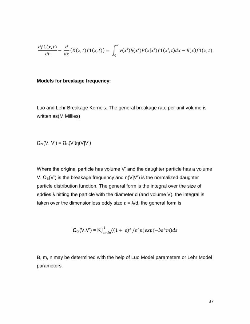
The population balance equation for the breakage process then becomes

37

( )

( ) ( ) = ( ) ( ) ( ) ( ) ( ) ( )

Models for breakage frequency:

Luo and Lehr Breakage Kernels: The general breakage rate per unit volume is

written as(M Millies)

Ωbr(V, V’) = ΩB(V’)η(V|V’)

Where the original particle has volume V’ and the daughter particle has a volume

V. ΩB(V’) is the breakage frequency and η(V|V’) is the normalized daughter

particle distribution function. The general form is the integral over the size of

eddies λ hitting the particle with the diameter d (and volume V). the integral is

taken over the dimensionless eddy size ε = λ/d. the general form is

Ωbr(V,V’) = K (( )

/ ) ( )

B, m, n may be determined with the help of Luo Model parameters or Lehr Model

parameters.

38

Coulaloglou and Tavlarides model: the breakage frequency was defined as the

fraction of particles breaking divided by a characteristic time. Thus

( ) = ( )

( ) (CA Coultalogou)

where, b is the breakage frequency, ε is the characteristic parameter (eg.

Volume) tb is the characteristic time and ∆F(ε)/ F(ε) is the fraction of particles

breaking(CA Coultalogou).

Furthermore,

∆F(ε)/ F(ε) = exp(-Ec/E)

With Ec being the surface energy and E the mean turbulent kinetic energy.

Also(CA Coultalogou),

Tb ∞ ε2/3 ε-1/3

Ghadiri breakage Kernels: this model is used to calculate only the breakage frequency.

The breakage frequency, f is related to the material properties and impact conditions(M

Ghadiri):

39

=

=

Where ρs is the particle density, E is the elastic modulus of the granule, and Γ is

the interface energy. ν is the impact velocity and L is the particle diameter prior to

breaking. Kb is the breakage constant and is defined as

=

Aggregation processes:

Aggregation must occur at least between two particles. It covers a variety of

processes ranging from coalescence in which two particles completely merge

along with their interiors, to coagulation, which features a “floc” of particles

loosely held by surface forces without involving physical contact. In intermediate

situations particles may be in physical contact with each other without merger of

their interiors(Ramakrishna).

The Aggregation Frequency: The aggregation frequency represents the

probability per unit time of a pair of particles of specified states aggregating. Let

the aggregating particles be described by the state vector (x, r) in a continuous

phase of state Y. The probabiltity that a particle at state (x, r) and another particle

40

at state (x’, r’), both present at time t will aggregate in the time interval t to t + ∆t

is given as(Ramakrishna)

a(x, r;x’, r’; Y, t)dt

Alternatively, a(x, r;x’, r’; Y, t) may be considered the fraction of particle pairs of

states (x, r) and (x’, r’) aggregating per unit time.

a(x, r;x’, r’; Y, t) satisfies the symmetry property

a(x, r;x’, r’; Y, t) = a(x’, r’;x, r; Y, t)

Consider a population of particles distributed according to their masses (or

volumes), denoted x. the aggregation frequency for particle masses x and x’ is

a(x, x’). The source term for formation of particles through aggregation is given

as (Ramakrishna)

h+(x, t) =

( ) ( t)d

the sink term for formation of particles through aggregation is given

as(Ramakrishna)

41

h-(x, t) = ( ) ( ) ( t)d

Aggregation Kernels:

Luo Aggregation kernel: The general aggregation kernel (Luo) is defined as the

rate of particle volume formation as a result of binary collisions of particles with

volumes Vi and Vj

Ωag(Vi, Vj) = ωag(Vi, Vj)Pag(Vi, Vj)

Where ωag(Vi, Vj) is the frequency of collision anf Pag(Vi, Vj) is the probability that

the collision results in coalescence. The frequency is defined as follows:

ωag(Vi, Vj) = (π/4)(di2 + dj

2)ninjuij

where uij is the characteristic velocity of collision of two particles with diameters di

and dj and the number densities ni and nj.

uij = (ui2 + uj

2)1/2

where

ui = 1.43(εdi)1/3

42

the expression for the probability of aggregation is

=

Where ci is a constant of order unity , xij = di/dj, ρ1 and ρ2 are the densities of the

primary and secondary phases, respectively and the weber number is defined as

=

Free Molecular Aggregation Kernel: Real particles aggregate with frequencies

characterized by complex dependencies over particle internal

coordinates(Schmoluchowski). Very small particles aggregate because of

collisions due to Brownian motion. In this case the frequency of collision is size

dependent and usually the following kernel is implemented.

= k

3

43

where kB is the Boltzmann constant, T is the absolute temperature, μ is the

viscosity of the suspending fluid.

44

SOLUTION METHODS FOR POPULATION BALANCE EQUATIONS

Method of classes:

This method discretizes the size domain in N intervals in a free of choice grid.

Due to this discretization one obtains a complete set of N ordinary differential

equations (ODE) which can be solved numerically.

Hounslow Ryall et al applied discretization techniques to the modeling of in-vitro

growth and aggregation of Kidney stones(MJ Hounslow).

John and Suciu employed discretization techniques to the solution of a bi-variate

population balance model for the nucleation and growth of Potassium

Dihydrogen Phosphate (KDP) particles(Volker John).

Consider the following one dimensional PBE

( )

( ( ) ( ))

= ( ) ( ) ( ) ( ) ( ) ( )

For simplicity, let us assume G(V, t) = G and γ(V) = 2

Consider the particle growth term ( ( ) ( ))

. This can be written

as(Ramakrishna)

(G ( t))

45

= ( ) ( )

Similarly, the breakage birth term ( ) ( ) ( ) ( )

may be

written as

( )

And, the breakage death term ( ) ( ) may be written as ( ) ( ).The

PBE is then converted into a system of N ordinary differential equations (ODEs)

given as(Ramakrishna)

( )

=

( ) ( )

( )

( ) ( )

Method of Moments:

The moment of the number distribution f is defined as:

( ) = ( )

(Ramakrishna)

The zeroth moment represents the total number of particles. The total volume of

the particulate phase is inferred from the first moment (j = 1) if the volume V is

chosen as the internal coordinate. Consider the following PBE

( )

( ( ) ( ))

= ( ) ( ) ( ) ( ) ( ) ( )

46

We need to transform the above equation into a set of ODEs. For this purpose,

we first multiply the equation by Vj, and then integrate from 0 to ∞. Thus, for the

first term

( )

= ( )

For the growth term,

( ( ) ( ))

=

For the breakage birth term

( ) ( ) ( ) ( )

=

( ) ( )

For the breakage death term,

47

( ) ( ) =

Thus, the PBE now becomes

( )

=

Where =

48

CASE STUDY - ONE DIMENSIONAL POPULATION BALANCE

MODEL OF A BATCH COOLING CRYSTALLIZATION PROCESS

A seeded batch cooling crystallization process of model Active Pharmaceutical

Incipient (API) in a model solvent was considered as a case study for the

development of a Population Balance Mode simulation and a solver was

developed in MATLAB. The relevant material properties and process settings are

described in the following table.

Material constants Value Description

Molecular weight API = 6 / Molecular weight of acetylsalicylic acid

(Aspirin®)

Molecular weight solvent = 6 / Molecular weight of ethanol

Density crystalline phase = / For simplification we assume an equal

density for the crystalline phase, the

pure solvent and the solvent containing

dissolved species of the crystalline

phase

Density pure solvent = /

Density solvent with

dissolved species = /

Reactor volume = In the present work We used the same

the initial mass for the solvent and the

API (solid & dissolved) for all

simulated experiments

Overall mass of pure solvent

in the reactor =

Overall mass of API in the

reactor =

49

In this case study only crystal growth was considered. Aggregation and breakage

were not considered in the simulation.

To establish the solubility of model API in model solvent the solubility of

acetylsalicylic acid dissolved in pure ethanol was used. This is given by the

following equation.

= ( )

Where N1 = 27.769, N2 = -2500.906 and N3 = -8.323(GD Maia).

The supersaturation is defined as

= /

/

Where c* is the solubility of API in the solvent and c is the current concentration.

A common size independent growth rate shown below is used for the model

under study(AD Randolph, Theory of Particulate Processes)(Mersmann)

( ) =

( )

50

The parameters for the above equation are given below(Mersmann), (AD

Randolph, Theory of Particulate Processes)

Model parameters (growth) value

=

=

=

The initial seed mass of the model API mcp initial and the initial concentration of

dissolved species cAPI initial depend only on the solubility as the initial temperature

Tinitial.

c

=

( )

( ( )) ( ) )

k = c

The total mass of the API in the system, mcp0 is assumed to be 500g. the initial

CSD was assumed to be a logarithmic distribution as follows.

( ) =

( / )

51

Where σln = 0.4 and L50 = 100μm. Furthermore, crystals were assumed to be

cubic and were defined by their characteristic lengths L. Thus, the following

constraint involving mcp may be imposed.

( )

For the current simulation L was varied from 0 to 400μm. This relation

was used for the normalization of the initial assumed distribution.

Thus, if the normalization constant was assumed to be con,

( )

=

Process settings of simulation experiments :

Tinitial [oC] = 45

mcpinitial = 0.388

tprocess = 1666

52

Discretization was employed for the solution of the resulting population balance

equations. The characteristic length L was varied from 1 to 400μm with a step

size of 1. Thus the PBE given as

( )

( ( ) ( ))

=

Was discretized as

( )

=

( ( ) ( ))

( )

53

Results:

The initial and final crystal size distribution is given as follows.

54

The supersaturation profile is shown as follows

55

The following graph validates the simulation through mass balance. It can be

seen that total mass of the system remains constant at 500g. This is the initial

assumed total mass of the system.

56

CONCLUSION

This report consists of a literature review of crystallization and Population

Balance Modeling followed by a case study of a crystallization process. This has

helped me gain a good knowledge base in PBM techniques so that I may pursue

further research in the field. In the case study a one dimensional PBM was

employed. I aim to work with multi-dimensional PBM simulations in the future.

Through the course of my research at TU Graz I have gained a starting point for

the research I aim to pursue during my Masters course at Rutgers University.

57

BIBLIOGRAPHY

AD Randolph, MA Larson. Theory of Particulate Processes. New York: Academic Press, 1998.

—. Theory of Particulate Processes (2nd Edition). New York: Academic Press, 1988.

AW Adamson, AP Gast. Physical Chemistry of Surfaces. New York: John Wiley and Sons, 1997.

CA Coultalogou, LL Tavlarides. "Description of interaction processes in agitated liquid–liquid

dispersions." Chemical Engineerinf Science (1977): 1289-1297.

Caliane Bastos Borba Costa, Maria Regina Wolf Maciel, Rubens Maciel Filho. "Considerations on

the crystallization modeling: Population balance solution." Computers and Chemical

Engineering (2007): 206-218.

D Ghosh, A Manka, R Strey, S Seifert, RE Winans and BE Wyslouzil. "Using small angle x-ray

scattering to measure the homogeneous nucleation rates of n-propanol, n-butanol, and

n-pentanol in supersonic nozzle expansions." The Journal of Chemical Physics (2008).

F Puel, G Fevotte, JP Kline. "Simulation and analysis of industrial crystallization processes

through multidimensional population balance equations. Part 1: a resolution algorithm

based on the method of classes." Chemical Engineering Science (2003): 3715-3727.

G Teqze, L Granasy, GI Toth, F Podmaiczky, A Jaatinen, T Ala-Nissila, T Pusztai. "Diffusion-

controlled anisotropic growth of stable and metastable crystal polymorphs in the phase-

field crystal model." PubMed (2009).

GD Maia, M Giulietti. Journal of Chemical and Engineering Data (2008).

HM Hulbert, S Katz. "Some problems in particle technology. A statistical mechanical

formulation." Chemical Engineering Science (1964): 555-574.

Kaoutar Abbou Oucherif, Shweta Raina, Lynne S. Taylor and James Litster. "Quantitative analysis

of the inhibitory effect of HPMC on felodipine crystallization kinetics using population

balance modeling." CrystEngComm (2013): 2197-2205.

Luo, H. Coalescence, Breakup and Liquid Circulation in Bubble Column Reactors. PhD thesis from

the Norwegian Institute of Technology. Trondheim, Norway, 1993.

M Ghadiri, Z Zhang. "Impact Attrition of Particulate Solids Part 1. A Theoretical Model of

Chipping." Chemical Engineering Science (2002): 3659-3669.

58

M Millies, D Mewes. "Bubble-Size Distributions and Flow Fields in Bubble Columns." AIChE

(2002): 2426-2443.

Mersmann, A. Crystalline Technology Handbook. n.d.

MJ Hounslow, RL Ryall, VR Marshall. "Discretized Population Balance for Nucleation, Growth,

and Aggregation." AIChE November 1988: 1821-1832.

Mullin, J.W. Crystallization. n.d.

NA Clontz, WL McCabe. "Contact Nucleation for MgSO4.7H2O." Chemical Engineering Progress

Symposium Series (1971): 6-17.

Nielsen, AE. Kinetics of Precipitation. Oxford and New York: Pergamon Press, 1964.

Ramakrishna, Doraiswamy. Population Balances-Theory and applications to Particulate Systems

in Chemical Engineering. Academic Press, 2000.

RC Miller, RJ Anderson, JL Kassner Jr, DE Hagen. "Homogeneous nucleation rate measurements

for water over a wide range of temperature and nucleation rate." The Journal of

Chemical Physics (1983).

RW Rousseau, KK Li, WL McCabe. "The influence of seed crystal size on nucleation rates." AIChE

Symposium Series (1976): 48-52.

Schmoluchowski, M. "Versuch Einen Mathematischen Theorie der Koagulationstechnik Kolloider

Lösungen." Zeitschrift für Physikalische Chemie (1917): 129-168.

Volker John, Carina Suciu. "Direct discretizations of bi-variate population balance systems with

finite difference schemes of different order." Chemical Engineering Science March 2014:

39-52.

Vonnegaut, B. "Variation with temperature of the nucleation rate of supercooled liquid tin and

water drops." Journal of Colloidal Science (1948): 563-569.

Y Ma Chao, Z Xue, Wang. "Model identification of crystal facet growth kinetics in morphological

population balance modeling of l-glutamic acid crystallization and experimental

validation." Chemical Engineering Science (2012): 22-30.