a study of rdb-based rdf data management techniques

A Study of RDB-Based RDF Data

Management Techniques

Vahid Jalali, Mo Zhou, and Yuqing Wu

School of Informatics and Computing, Indiana University, Bloomington{vjalalib,mozhou,yugwu}@indiana.edu

Abstract. RDF has gained great interest in both academia and indus-try as an important language to describe graph data. Several approacheshave been proposed for storing and querying RDF data efficiently; eachworks best under certain circumstances, e.g. certain types of data and/orqueries. However, there was lack of a thorough understanding of exactlywhat these circumstances are, as different data-sets and query sets areused in the empirical evaluations in the literature to highlight their pro-posed techniques. In this work, we capture the characteristics of dataand queries that are critical to the RDF storage and query evaluationefficiency and provide a thorough analysis of the existing storage, index-ing and query evaluation techniques based on these characteristics. Webelieve that our study not only can be used in evaluating both existingand emerging RDF data management techniques, but also lays the foun-dations for designing RDF benchmarks for more in-depth performanceanalysis of RDF data management systems.

Keywords: RDF, SPARQL, Storage, Index, Query Evaluation.

1 Introduction

Resource Description Framework (RDF) [3] which is a World Wide Web Con-sortium (W3C) recommended standard, represents data entities and their rela-tionships in the Semantic Web. In RDF, each data entity has a Unique ResourceIdentifier (URI) and each relationship between two data entities is describedvia a triple within which the items take the roles of subject(S), predicate (orproperty)(P) and object(O). RDF Schema (RDFS) [6] further extends RDF todescribe the semantic and structure of the data by introducing classes.

A B C

D

P

E

foaf foaf

coauthor

foaf

siste

r

typetype

type type

type A: AmyB: BobC: ChrisD: DanE: EllenP: People

K

DBMS Concept

like

nam

e

Fig. 1. Example RDF data

Fig. 1 shows a graph representa-tion of a sample RDF data and itsschema that describes people, booksand their relationship in social net-works. The arch “Amy type Person”indicates that Amy is an instance ofthe class named “Person”.

SPARQL [9] is an RDF querylanguage recommended by W3C to

H. Wang et al. (Eds.): WAIM 2011, LNCS 6897, pp. 366–378, 2011.c© Springer-Verlag Berlin Heidelberg 2011

A Study of RDB-Based RDF Data Management Techniques 367

facilitate users to retrieve meaningful information from RDF data. A SPARQLquery consists of graph pattern(s) that can identify the nodes/edges of interestthrough graph pattern matching against the RDF data. The following queryretrieves a person who is a friend of A, and his/her relationship with B is thesame as D’s relationship with E.

SELECT ?person WHERE {?person foaf A . ?person ?p B. D ?p E}To keep pace with the ever-increasing volume of semantic web data and the needsof answering complicated queries on such data, various RDF storage methodswere proposed to improve the RDF data storage and query evaluation efficiency.Majority of these approaches rely on existing relational database (RDB) man-agement systems, among which the most notable techniques are Triple Store [7],Vertical Partitioning [4] and Property Table [19]. Indexing methods were alsoinvestigated, including MAP [10], Hexastore [18] and TripleT [8].

It is the general wisdom that engineering designs all have their advantagesand drawbacks; they are superb for certain circumstances but less so for others.Benchmarks, which consist of both data set and query set, are designed to helpusers determine the strength and limitations of a data management system or aspecific data management technique. In the context of RDF, many efforts [14,15]have been made in this regard. However the question “what characteristics ofdata and query highlight the advantages and drawbacks of a storage method” isyet to be answered, as existing benchmarks are not yet covering key character-istics of RDF data and queries, especially those that bring challenges to RDFstorage and query evaluation techniques.

We set out to conduct such a thorough analysis, focusing on the type ofdata and queries that are not well covered (e.g. the sample query above) by theexisting benchmarks and studies. In particular,

– We introduce and analyze a set of key characteristics of RDF data for ana-lyzing the space efficiency of RDF storage methods.

– We classify SPARQL queries based on roles of the variables, and identify thechallenges brought by data storage and query evaluation techniques.

– We design extensive empirical study to investigate and compare existingRDF data management techniques, and prove that the data and query char-acteristics we identified are indeed critical.

– We analyze existing RDF benchmarks based on the data and query charac-teristics we propose, and suggest improvement in RDF benchmark designing.

2 Storage Efficiency

In this section, we study the space efficiency, i.e. the amount of space required forstoring RDF data, of different RDB-based RDF data storage methods, specifi-cally nonindex-based and index-based methods.

Definition 1. Given an RDF document D in triple format, and a data storageor indexing method M that is designed to store D, the storage efficiency of M

368 V. Jalali, M. Zhou, and Y. Wu

with respect to document D is SEDM = SM(D)

S(D) , where S(D) represents the size ofthe text document D in triple format, and SM(D) represents the space requiredfor storing D using method M.

Obviously, the smaller the value of SEDM, the better method M is for stor-

ing/indexing document D. In the rest of this section, we study the most promi-nent RDF data storage and indexing techniques in the literature, identify keycharacteristics of RDF data that determine the storage requirement, and proposeformulas for calculating SM(D) for each method. Then, we will report the resultof our impartial study on the storage efficiency of these techniques, w.r.t. RDFdocuments with various combinational configurations on the key characteristics.

2.1 RDF Data Storage Methods

The most prominent RDF data storage methods are Triple Store (TS) [7], Ver-tical Partitioning (VP) [4] and Property Table (PT) [19]. Fig. 2 illustrates howthese three methods store some fragments of the RDF data whose graph repre-sentation was shown in Fig. 1.

Subject Predicate ObjectA type P Subject Object Subject Object Subject Name foafD type P A P A D A "Amy" DK type Book D P D "Dan" NullA foaf D K BookK name "DBMS�Concepts" Subject ObjectA name "Amy" K "DBMS�Concepts" SubjectD name "Dan" A "Amy" K

D "Dan"

Triple�StoreType foaf

name

Vertical�Partitioning Property�Table

Name"DBMS�Concepts"

Book

P�

Fig. 2. The Sample Data Stored in TS, VP and PT

Data Schema OverheadTS 3×|D|×L OT S

VP 2×|D|×L |pred(D)|×OV P

PT (|D|-|lft(D)|)×L +3×|lft(D)|×L |cls(D)|×OPT +OT S

The space requirementsof these storage methodsare shown in the table onthe right. We use |D| to rep-resent the total number of triples in D and L the average size of all values in D,while the other data characteristics and how they impact the storage efficiencyof a data storage method will be discussed in details next.

In Triple Store [7], all triples are stored in a single table with three columns(S, P, O). Therefore, the space requirement is determined by the number oftuples in that table, e.g. the number of triples in the RDF data (|D|), and thesize of each value to be stored. The only overhead (OTS) is for storing the schemaof the triple store table in the system catalog.

In Vertical Partitioning [4], a separate table is created for each distinctpredicate to store all triples that feature this predicate. As all triples in eachtable share the same predicate, the predicate is omitted and only the valuesof the subject and object roles are stored. Therefore, the space requirement isdetermined by the number of tuples in these tables, as well as the number oftables, which is the number of unique predicates in the RDF data (|pred(D)|).


The overhead (OV P ) is incurred by storing the schema of each VP table, whichincreases as |pred(D)| increases.

In Property Table [19], RDF data are stored in traditional relational tableswhose schema carry the semantics of the residential data. There are two types ofPTs that provide distinct ways in shredding RDF triples into tables: (1) ClusteredProperty Table, in which RDF triples with the subjects sharing the same set ofpredicates are clustered into a property table, generated manually, or using adynamic lattice based method [17]; and (2) Property-class Table, in which atable is created for each class and stores information about all members of thatclass, with the attributes being the single-value predicates of these members. Inboth implementations, a leftover table with three columns (S, P, O) is createdfor storing the triples not belonging to any other tables. In the former method,the schema of the property tables highly depends on the clustering algorithms,which varies based on the implementations. Thus we focus on the latter methodin which the property tables are determined once the schema information isgiven. In the rest of the paper, when we refer to Property Table method, weare indeed referring to the property-class table method. In contrast to verticalpartitioning and triple store, it is not straightforward to decide the schema ofthe tables used for storing RDF data in property tables.

The space requirement for PT method consists of two parts: the space requiredfor storing the property tables and the space required for storing the leftovertable, each of which, similar to our discussion of the TS and VP methods, consistsof a data component and a schema component. The number of property tablesis the number of classes (|cls(D)|). |lft(D)| represents the number of triples thatcannot be placed in any property table but have to be placed in the leftover table.The overhead for each property table is denoted by OPT , while the overhead ofthe leftover table is the same as a triple store table, OTS .

OT S = O + 3 × C

OV p = O + 2 × C

OP T = O + (avgPred(D) + 1) × C

Assuming the space required for storingthe information of each attribute in the sys-tem catalog is the same, denoted C, and theoverhead for storing the information of a ta-ble is the same, denoted O, then, the over-head for storing the schema information, referred to as OTS , OV P and OPT inthe table above, can be further depicted using the formula on the right. Here,avgPred(D) represents the average number of single-value predicates of eachclass. Note that in the PT method, besides the attributes that correspond tothe single-value predicates of each class, an additional attribute is introduced tostore the URIs of the subjects.

2.2 Index-Based Storage Methods

To facilitate efficient query answering, multiple indexing techniques were pro-posed, including MAP [10], Hexastore [18] and TripleT [8], whose structures areillustrated in Fig. 3. Indeed the index-based methods proposed are not merelydesigns of indices but alternative ways for storing RDF data for efficient dataaccessing based on indexing techniques. Hence, we call them index-based storagemethods.


<k1k2k3> ... ... ...

(a) MAP

<k1k2> ... ...

k.

.

.

...

(b) HexTree

<k> ......

k1k2

.

.

.

...

(c) TripleT

Fig. 3. RDF Indices [8]

Before we discuss thespace requirement of theindex-based storage meth-ods, we review the spacerequirement of a tradi-tional clustered B+-tree in-dex. Given the number ofunique values of the indexkey Nk, the data size of theindex key Sk, the size of apointer Sptr, and the size a page SP (assume that Sptr and SP are fixed), the

space requirements of the B+-tree is SBT (Nk, Sk) = SP ×logf Nk∑

i=1

f i, where the

fan-out f is computed as f = SP

Sk+Sptr.

The space requirement of each index-based storage method consists of twoparts: (1) the space requirement of the clustered B+-tree indices; and(2) thespace requirement of the payload pointed by the leaf nodes in B+-tree indices.We summarize these in the table below.

Payload IndexMAP 0 6× SBT (|D|, 3 × L)

Hexastore∑

role={S,P,O}|πroleD| × L 6×

∑

role={SP,SO,P O}SBT (|πroleD|, 2 × L)

TripleT 3 × |val(D)| × L SBT (|val(D)|, L)

MAP [10] builds six clustered B+-tree indices on six RDF triple store tables,each clustered on one permutation of S, P and O, i.e. SPO, SOP, PSO, POS,OSP, OPS. As a result, all RDF triples are stored six times on the leaf nodes ofthese indices. On each such replication a B+-tree index is built, with Nk=|D| andSk=3× L. Please note that there is no additional payload as all three roles areindexed. More recently, MAP method was enhanced by indexing over aggregatedfunctions and by using index compression techniques [13].

Hexastore [18] improves the storage efficiency of MAP by reducing the spacerequirement of the index part and the duplication of the RDF data. Instead ofindexing all three roles, Hexastore builds six clustered B+-tree indices on twoout of three roles of RDF triples, i.e. SP, PS, SO, OS, PO, OP, while the twoindices on symmetric roles, e.g. SP and PS, share the same payload that containsthe distinct values of the other role, in this case O. In the worst case, the RDFtriples are duplicated five times.

Rather than creating six B+-tree indices, TripleT [8] uses only one B+-treeto index all distinct values in an RDF document, across all roles. Each leaf nodein this B+-tree has a payload that is split into three buckets, S, P and O, andeach bucket holds the list of related atoms for the other two roles. Thereforethe space requirement of TripleT is the sum of (1) the overall payload, in whicheach triple in the RDF data is stored 3 times, one under its subject’s value, one


under its predicate’s value, and one under its object’s value; and (2) the size ofa single B+-tree index.

2.3 RDF Data Characteristics

Based on the analysis above, we identify the following as key factors that canbe used to describe the characteristics of an RDF data D and to evaluate andmeasure the space efficiency of RDF data storage and indexing techniques.

1. |D|: the total number of triples in D;2. |pred(D)|: the number of unique properties in D;3. |val(D)|: the number of unique values in D;4. |cls(D)|: the number of classes in D;5. avgPred(D): the average number of properties belonging to the same class

in D; and6. |lft(D)|: the number of triples whose subjects do not belong to any class or

whose predicates are multi-value predicates.

As the values of (2), (3), (4) and (6) partially depend on the value of (1), indeed,it is the ratio of these values to |D| that truly describes the data distribution ofan RDF data. Also note that there is correlation between |D|, |pred(D)|, |cls(D)|and avgPred(D). Even though there is no direct functional relationship betweenthem, but given three, a tight up/lower bound is set on the value the forth cantaken.

2.4 Data Characteristics in RDF Benchmarks

We have identified 6 key factors of RDF data that have significant impact onthe storage efficiency of RDF data storage and indexing techniques. We believeinsightful comparison of such techniques should be conducted on data-sets inwhich all the key factors vary.

Benchmark |pred(D)| |val(D)| |D| Used inBarton [5] 285 19M 50M [4,11,15,18]LUBM [2] 18 1M 7M [18]Yago [16] 93 34M 40M [11]

LibraryThing [1] 338824 9M 36M [11]

The data characteristics thatare covered by the existingbenchmarks that are used in theresearch work of RDF data stor-age and indexing is summarized in the table on the right. As the schema infor-mation is frequently absent from these benchmarks, we do not summarize theschema related data characteristics, namely |cls(D)|, avgPred(D) and |lft(D)|,in the table.

2.5 Empirical Analysis

To provide a thorough understanding of the storage methods, and answer thequestion about exactly what type of RDF data each storage method is best/worstat, we generate and conduct experiments on synthetic data sets, big and small,with various combination on the key factors we identified in Sec. 2.3. The trendwe observe are the same. In this section, we present our results on the comparison


based on multiple data sets with a fixed number of triples (100,000 triples to bespecific), but vary on other characteristics.

In order to better understand the correlation between |pred(D)| and storageefficiency of RDF repository that highlights the advantage and drawback of thePT method, we design our RDF data set such that all triples fit in propertytables and the leftover table is empty. Since a leftover table is nothing but atriple store table of the residential RDF triples, the storage efficiency of the PTmethods on data that yield non-empty leftover table can be easily estimated byintegrating the analysis and observations of both PT and TS methods.

We use MySQL to implement the storage methods discussed in Sec. 2.1 andSec. 2.2. Specifically, we use relational tables and B+-tree indices to implementthe three index-based storage methods discussed in Sec. 2.2, by storing the RDFtriples in their proper clustering order in relational tables and create B+-treeindices on top of these tables, hence the key concepts and features of the originalmethods are loyally preserved.

0

2

4

6

8

spaceefficiency(lo

g)

TS

VP

PT (Min)

PT (Avg)

2

0

2

4

6

8

0.00001 0.0001 0.00247 0.01 0.1 1

spaceefficiency(lo

g)

|pred(D)|/|D|

TS

VP

PT (Min)

PT (Avg)

PT (Max)

Fig. 4. Space Efficiency Comparison:Data Storage Methods

Data Storage Methods. The im-pact of the number of unique predicates(|pred(D)|) on the space efficiency of thedata storage methods is shown in Fig. 4. Asthe value of |pred(D)| is strongly correlatedto the number of triples in an RDF docu-ment, we use the ratio, |pred(D)|

|D| as the pa-rameter. Please note that logarithmic scaleis used on the y-axis, due to the large dif-ference exhibited by different methods.

Reflecting our analysis presented in Sec. 2.1, TS is indifferent to |pred(D)|.SED

V P is heavily affected by |pred(D)| because the larger |pred(D)| is, thegreater the overhead for storing the schema info of the tables would be. VP,originally designed to improve the space efficiency of TS, can end up to be notefficient, even very inefficient, when the overhead is driven up by large numberof unique predicates, cancelling out the saving of not storing the predicate valuein those tables.

Fig. 5. Storage Efficiency Analysis: Property Table

The impact of|pred(D)| varieson PT, in whichother factors playmore importantroles on the spaceefficiency. In Fig. 4,PT (Max), PT (Avg)and PT (Min) represent the maximum, average and minimum storage efficiencywe obtained on various RDF data sets that share the same |pred(D)|. We theninvestigate the impact of other factors, including the number of classes (|cls(D)|)and average number of predicates per class (avgPred(D)), on PT method.

As seen in Fig. 5(a), indeed |pred(D)| does not have any direct impact onSED

PT . It only defines what the values of avgPred(D) and |cls(D)| may be.


For RDF documents with the same |pred(D)|, SEDV P are different when

avgPred(D) and |cls(D)| are different. When |D| and |cls(D)| are fixed, thedirect impact of avgPred(D) on SED

PT is illustrated in Fig. 5(b). The curvereflects the trade-off between the save in data storage by introducing widerproperty tables and the overhead in storing the schema info of all the columnsin the wider tables.

Fig. 6. Storage EfficiencyComparison: Indexing

Index-based Storage Methods. We store RDFdata of various |val(D)|/|D| ratio using the threeindex-based storage methods. Our experimental re-sults, as shown in Fig. 6, confirm our analysis. Assummarized in Sec. 2.2, space efficiency wise, the dif-ference between MAP and Hexastore lies in the sizeof the index tree and index leaf nodes. Hence, Hexas-tore is always more space efficient than MAP. TripleTdistinguishes itself from MAP and Hexastore by in-dexing only unique values. Therefore, the unique number of values in the RDFdata is the dominating factor of the space efficiency of TripleT. In addition, as itstores each triple only three times, in most cases it is more efficient than MAPand Hexastore. However, it becomes less efficient when the number of uniquevalues increases.

3 Query Evaluation

As a matter of fact, data storage and indexing techniques are invented to facil-itate efficient query evaluation. Hence, besides space efficiency, query efficiencyis of ultimate importance.

3.1 Query Patterns

SPARQL [9],recommended by W3C, is the de facto standard RDF query lan-guage. A SPARQL query consists of one or more graph patterns, the evaluationof which is based on graph pattern matching against the RDF data graph. LetL be a finite set of literals, U a finite set of URIs and V a finite set of variables.Then an RDF triple is in the set U × U × (U ∪ L) and a simple triple pattern(STP) in a SPARQL query is in the set (U ∪V)× (U ∪V)× (U ∪ V ∪L). Pleasenote that a variable can appear in the role of subject, predicate, or object.

s,type, ?o s, p, ?o s, ?p, o ?s, p, o ?s, type, o

?s,type,?o ?s, p, ?o ?s, ?p, o s, ?p, ?o ?s, ?p, ?o

We list 10 different simpletriple patterns based on thenumber and roles of variables ina pattern. Specifically we distinguish “type” from other predicates, becausematching the pattern (?s, type, o) is very different from (?s, p, o) in PropertyTable as the knowledge of the class that ?s belongs to can determine the prop-erty table to search in, while the knowledge of the constant p can not have thesame filtering effect on the optimization process.

A graph pattern (GP) is a non-empty set of STPs. We define a connectedgraph pattern recursively as follows.


Definition 2. A graph pattern with single STP is connected. If two connectedgraph patterns, g1 and g2, share a common variable or URI, we say that thegraph pattern g3 = g1 ∪ g2 is also connected.

Please note that our classifications of whether a graph pattern is connectedmerely depends on whether the STPs share variables or URIs, not whether thegraph pattern, when represented as a graph, is a connected graph. For instance,in our classification, {s1,?p,o1. s2, ?p, o2} is a connected graph pattern.

Join type Example

S-S ?s p1 o1. ?s p2 o2

O-P s1 p1 ?x. s2 ?x o2

O-O s1 p1 ?o. s2 p2 ?o

P-P s1 ?p o1. s2 ?p o2

S-O ?x p1 o1. s2 p2 ?x

S-P ?x p1 o1. s2 ?x o2

We call a connected graph pattern single jointgraph pattern (SJGP) if it has exactly two STPs.Based on the roles that the shared variable takes inthese STPs, we can identify six types of joins.

Definition 3. Given a SJGP, g = {stp1, stp2},where stp1 = (s1, p1, o1) and stp2 = (s2, p2, o2).We say that g is formed by S-S join if s1, s2 ∈ Vand s1 = s2. Similarly we can define O-O, S-O, P-P, S-P, and O-P joins.

A graph pattern may consist of multiple STPs, multiple variables and multipletypes of joins. We call them Complex Join Patterns (CJP). To better understandhow CJPs can be evaluated by different storage methods, it would be beneficialto first understand how many types of CJPs there are.

[12] defined chain shape patterns (CSP) as a set of STPs linked together viaS-O joins and star shape pattern (SSP) as a set of STPs linked together via S-Sjoins. They proved that all data storage approaches do not favor queries withCSP and PT favors queries with SSP.

However, CSP and SSP as defined in [12] represent only a very small fragmentof SPARQL queries. In this paper we propose a more sophisticated classificationbased on the positions of variables in a graph pattern, which extends the conceptsof CSP and SSP by (1) considering all positions of variables, i.e. S, P and O; and(2) considering all types of joins besides S-S join in SSP and S-O join in CSP.

Definition 4. Given a connected graph pattern gp that consists of more thantwo STPS, we say that gp is:– an Extended Chain-shaped Pattern(ECP) if no more than two STPs in gp

share a common variable;– an Extended Star-shaped Pattern (ESP) if all STPs in gp share at least one

common variable;– a Hybrid Pattern (HP) if gp does not fall into the above categories.

The graph pattern in the query we presented in Sec. 1, {?person foaf A .?person ?p ?person. D ?p E }, is an ECP, featuring a S-S join and a P-P join.

3.2 Query Patterns in Benchmarks

The design of the query set in a benchmark plays a critical role in testing howefficiently a data management system can handle various types of queries. Wesummarize the query patterns (STP, SJP and CJP) that are covered by existingbenchmarks.


Benchmark STP SJP CJP Used inBarton [5] ?s type o, ?s type ?o, S-S, S-O SSP, CSP [4,11,15,18]

?s p o, ?s p ?o, ?s ?p ?oLUBM [2] ?s p o, ?s p ?o S-O, O-O None [18]Yago [16] ?s type o, ?s p o, S-S, S-O, O-O SSP, CSP [11]

?s p ?o, ?s ?p ?oLibraryThing [1] ?s p o, ?s p ?o S-S, S-O, O-O SSP [11]

Our obser-vations are:(1) Querieswith variablesin the predi-cate role arenot well ex-plored. When the lone query with ?p in Barton was used, it was applied toan RDF data with only 28 unique predicates [4]. (2) The queries in each bench-mark cover at most three different SJPs, and none of them feature any join thatinvolves a variable in the predicate role. (3) The queries in these benchmarks areas complex as SSP and CSP, but none of the benchmark features any extendedjoin patterns we defined, which, as shown in our motivating example in Sec. 1 isa typical query that appear in real life applications.

3.3 Empirical Study

To better understand how the RDF data storage and index-based storage tech-niques proposed in the literature stand up to the challenges of the importanttypes of query patterns, we designed a set of queries to stress the systems.

|D| |pred(D)| |val(D)| |cls(D)| avgPred(D) |lft(D)|10M 900 1.7M 100 10 0

The data characteristics of oursynthesized data-set is shown onthe right. This data set is chosenas it does not favor one data storage and/or index-based storage method overanother, in terms of space efficiency. |lft(D)| is 0, in order to weed out theimpact of the leftover table when we evaluate the query evaluation performanceof PT.

Query Pattern |Result|STP1 ?s p o 1KSTP2 ?s type o 1KSTP3 s ?p o 1KSTP4 s ?p o 22STP5 ?s ?p o 1KSJP1 ?x p1 o1. ?x p2 o2 1KSJP2 s1 p1 ?x. s2 ?x o1 1KESP1 s1 ?x o1. s2 ?x o2. s3 ?x o3 100ECP1 s1 p1 ?x. ?x ?y o1 . s2 ?y o2 100

We have tested on large numberof queries, STPs, SJPs, and CJPs, ofvarious value/join selectivity and re-sult cardinality. We pick the querieson the right to illustrate our analysisand observations. The class a querybelongs to is reflected in its name.Query patterns and the result cardi-nalities of these queries are also provided.

Fig. 7. STP - Data Storage Methods

Simple TriplePatterns (STP).We first study howdifferent data stor-age methods fairanswering STPqueries. We focuson the missingpieces in theliterature and


investigate the impact of the certainty of the values in the predicate role onthe evaluation of STPs. As shown in Fig. 7(a), for STP1, VP outperforms TSand PT, since in VP, the search is limited to only the table corresponding to thegiven predicate, while the search in TS involves the full TS table, and the searchin PT involves multiple tables, corresponding to classes that feature the givenpredicate. In comparison, PT performs better when only one property table canbe identified, i.e. STP2, with the combination of “type” in the predicate role anda constant in the object role, as shown in Fig. 7(b). This impact is magnifiedwhen a variable is on the predicate role, i.e. STP3, as illustrated in Fig. 7(c). Forthis type of queries, TS outperforms VP and PT thanks to its simple schema,as in both VP and PT, all tables have to be searched to answer the query.

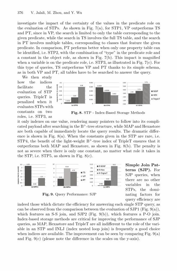
Fig. 8. STP - Index-Based Storage Methods

We then studyhow the indicesfacilitate theevaluation of STPqueries. TripleT ispenalized when itevaluates STPs withconstants on tworoles, i.e. STP3, asit only indexes on one value, rendering many pointers to follow into its compli-cated payload after searching in the B+-tree structure, while MAP and Hexastoreare both capable of immediately locate the query results. The dramatic differ-ence is shown in Fig. 8(a). When the constants given in the STP are rare, i.e.STP4, the benefit of the light-weight B+-tree index of TripleT ensures that itoutperforms both MAP and Hexastore, as shown in Fig. 8(b). The penalty isnot as severe when there is only one constant, no matter what role it takes inthe STP, i.e. STP5, as shown in Fig. 8(c).

Fig. 9. Query Performance: SJP

Simple Join Pat-terns (SJP). ForSJP queries, whenthere are no othervariables in theSTPs, the domi-nating factors forquery efficiency are

indeed those which dictate the efficiency for answering each single STP query, ascan be observed from the comparison between the evaluation of SJP1 (Fig. 9(a)),which features an S-S join, and SJP2 (Fig. 9(b)), which features a P-O join.Index-based storage methods are critical for improving the performance of SJPqueries, as MAP, Hexastore and TripleT are all indifferent to the role of the vari-able in an STP and INLJ (index nested loop join) is frequently a good choicewhen indices are available. The improvement can be seen by comparing Fig. 9(a)and Fig. 9(c) (please note the difference in the scales on the y-axis).


Fig. 10. Query Performance: CJP

Complex Join Patterns (CJP).As to the CJP queries, we focus onthe extended star and chain shapedpatterns (ESP and ECP) we iden-tified, especially the patterns thatwere not studied in the literature be-fore, for example, ESP1, a star pat-tern that join on predicate role, andECP2, a chain shaped pattern involving a P-P join.

As can be observed from Fig. 10(a), on ESP1, VP outperforms TS and PT.The reason is that when the predicate is unknown, in both TS and PT, all datahas to be searched then joined. However, in VP, to yield the final results, triplesin one table only need to join with other triples in the same table. In otherwords, the vertical partitioning serves as a pre-hashing. As it could be seen inFig. 10(b), VP and PT slightly outperform TS, as they both take advantage ofthe known predicate to narrow down the search in evaluating one STP. However,due to the uncertainty introduced by the variable in the predicate roles, theiradvantage over TS is not as obvious as if the query is a CSP with features onlyS-O joins. As the index-based storage methods are indifferent to the the rolesof the variable, adding more STPs and more joins only intensify what we haveobserved in the SJP cases.

4 Conclusion

Based on the in-depth study of the RDB-based RDF data storage and index-ing methods, we introduce a set of key data characteristics based on which wecompare the storage efficiency of these methods. We study SPARQL queries,introduce new ways to classify patterns based on the locations of the variables,and compare and analyze the query evaluation efficiency of the storage methods,focusing on the query patterns that were not in the RDF benchmarks and notreported in the literature.

Our empirical evaluation testify the law of engineering design: there is no one-size-fit-all method — each method is superb only for certain types of data andcertain types of queries. Our study also illustrates the insufficiency of existingRDF benchmarks for providing thorough and in-depth measurement of RDFdata management and query evaluation techniques. We believe that our anal-ysis and findings presented in this paper will serve as a guideline for designingbetter RDF benchmarks, which is indeed what we plan to pursue in the wake ofcompleting this project.

References

1. Librarything data-set, http://www.librarything.com/

2. LUBM data-set, http://swat.cse.lehigh.edu/projects/lubm/

http://www.librarything.com/

http://swat.cse.lehigh.edu/projects/lubm/


3. Resource Description Framework (RDF). Model and Syntax Specification. Techni-cal report, W3C

4. Abadi, D., et al.: Scalable Semantic Web Data Management Using Vertical Parti-tioning. In: VLDB, pp. 411–422 (2007)

5. Abadi, D., et al.: Using The Barton Libraries Dataset As An RDF Benchmark.Technical Report MIT-CSAIL-TR-2007-036, MIT (2007)

6. Brickley, D., et al.: Resource Description Framework (RDF) Schema Specification.W3C Recommendation (2000)

7. Broekstra, J., et al.: Sesame: A Generic Architecture for Storing and QueryingRDF and RDF Schema. In: Horrocks, I., Hendler, J. (eds.) ISWC 2002. LNCS,vol. 2342, pp. 54–68. Springer, Heidelberg (2002)

8. Fletcher, G., et al.: Scalable Indexing of RDF Graphs for Efficient Join Processing.In: CIKM, pp. 1513–1516 (2009)

9. Furche, T., et al.: RDF Querying: Language Constructs and Evaluation MethodsCompared. In: Barahona, P., Bry, F., Franconi, E., Henze, N., Sattler, U. (eds.)Reasoning Web 2006. LNCS, vol. 4126, pp. 1–52. Springer, Heidelberg (2006)

10. Harth, A., et al.: Optimized Index Structures for Querying RDF from the Web.In: LA-WEB, p. 71 (2005)

11. Neumann, T., et al.: RDF-3X: a RISC-style Engine for RDF. Proc. VLDB En-dow. 1(1), 647–659 (2008)

12. Neumann, T., et al.: Scalable Join Processing on Very Large RDF Graphs. In:SIGMOD, pp. 627–640 (2009)

13. Neumann, T., et al.: The RDF-3X engine for scalable management of RDF data.VLDB J. 19(1), 91–113 (2010)

14. Schmidt, M., et al.: SP 2 Bench: A SPARQL performance benchmark. In: ICDE,pp. 222–233 (2009)

15. Sidirourgos, L., et al.: Column-store Support for RDF Data Management: Not allSwans are White. Proc. VLDB Endow. 1, 1553–1563

16. Suchanek, F., et al.: YAGO: A Core of Semantic Knowledge - Unifying WordNetand Wikipedia. In: WWW, pp. 697–706 (2007)

17. Wang, Y., et al.: FlexTable: Using a Dynamic Relation Model to Store RDF Data.In: Kitagawa, H., Ishikawa, Y., Li, Q., Watanabe, C. (eds.) DASFAA 2010. LNCS,vol. 5981, pp. 580–594. Springer, Heidelberg (2010)

18. Weiss, C., et al.: Hexastore: Sextuple Indexing for Semantic Web Data Manage-ment. Proc. VLDB Endow. 1, 1008–1019 (2008)

19. Wilkinson, K., et al.: Jena Property Table Implementation. In: SSWS (2006)

a study of rdb-based rdf data management techniques

Documents