a study of semi-volatile toxic organic air pollutants · pdf filewe have read the thesis...
TRANSCRIPT

DOKUZ EYLÜL UNIVERSITY
GRADUATE SCHOOL OF NATURAL AND APPLIED
SCIENCES
A STUDY OF SEMI-VOLATILE TOXIC ORGANIC AIR POLLUTANTS IN ALİAĞA
HEAVY INDUSTRIAL REGION
by Ayşe BOZLAKER
July, 2008 İZMİR

A STUDY OF SEMI-VOLATILE TOXIC ORGANIC AIR POLLUTANTS IN ALİAĞA
HEAVY INDUSTRIAL REGION
A Thesis Submitted to the
Graduate School of Natural and Applied Sciences of Dokuz Eylül University
In Partial Fulfillment of the Requirements for the Degree of Doctor of
Philosophy in Environmental Engineering, Environmental Technology Program
by
Ayşe BOZLAKER
July, 2008 İZMİR

ii
Ph.D. THESIS EXAMINATION RESULT FORM
We have read the thesis entitled “A STUDY OF SEMI-VOLATILE TOXIC
ORGANIC AIR POLLUTANTS IN ALİAĞA HEAVY INDUSTRIAL
REGION” completed by AYŞE BOZLAKER under supervision of PROF. DR.
AYSEN MÜEZZİNOĞLU and we certify that in our opinion it is fully adequate, in
scope and in quality, as a thesis for the degree of Doctor of Philosophy.
Prof. Dr. Aysen MÜEZZİNOĞLU
Supervisor
Assoc. Prof. Dr. Mustafa ODABAŞI Assoc. Prof. Dr. Aysun SOFUOĞLU
Thesis Committee Member Thesis Committee Member
Prof. Dr. Gülen GÜLLÜ Prof. Dr. Abdurrahman BAYRAM
Examining Committee Member Examining Committee Member
Prof. Dr. Cahit HELVACI Director
Graduate School of Natural and Applied Sciences

iii
ACKNOWLEDGMENTS
I would like to express my sincere gratitude to my advisor Prof. Dr. Aysen
MUEZZINOGLU for her invaluable suggestions, guidance, and support during this
research and preparing thesis. I am also grateful to Assoc. Prof. Dr. Mustafa
ODABASI who has made a significant contribution to this study by giving advice,
guidance, and support. His encouragement and valuable advice often served to give
me a sense of direction during my studies. I would like to thank my other thesis
committee member Assoc. Prof. Dr. Aysun SOFUOGLU, and my examining
committee members, Prof. Dr. Abdurrahman BAYRAM and Prof. Dr. Gulen
GULLU, and Assoc. Prof. Dr. Sait SOFUOGLU for their helpful suggestions and
comments throughout this study.
I am thankful to Dr. Faruk DINCER (TUBITAK) for his assistance during air
sampling periods. I am also grateful to ENKA power station in Aliaga, Izmir for
allowing the use of their air pollution measurement station and meteorological data
generated at this site.
I would like to thank Dokuz Eylul University (Project No: 03.KB.FEN.101) for
the financial support to this study. I also thank all the members of Dokuz Eylul
University, Air Pollution Laboratory for their help during my laboratory studies.
Finally, I would like to express my deep appreciation to my family for their
understanding, support, patience, and encouragement during this study.
Ayse BOZLAKER

iv
A STUDY OF SEMI-VOLATILE TOXIC ORGANIC AIR POLLUTANTS IN
ALİAĞA HEAVY INDUSTRIAL REGION
ABSTRACT
Ambient air, dry deposition, and soil samples were collected during the summer
and winter periods at a sampling site close to the Aliaga industrial region in Izmir,
Turkey. Soil samples were also taken from additional 48 different sites around the
study area. All samples were investigated for SOCs (PAHs, PCBs, and OCPs).
Atmospheric PAH concentrations were higher in winter than in summer, indicating
that wintertime concentrations were affected by residential heating emissions. On the
contrary, increased atmospheric PCBs and OCP levels were observed in summer,
probably due to increased volatilization at higher temperatures and seasonal
agricultural applications of in-use pesticides. Low molecular weight PAHs
(phenanthrene, fluorene, fluoranthene) and PCBs (tri-, tetra-, penta-CBs) were the
most abundant compounds in air for both seasons. For OCPs, they were endosulfan-
I, endosulfan-II and chlorpyrifos in summer, and chlorpyrifos, α-HCH, and
endosulfan-I in winter, respectively. In contrast to PCBs, particulate fluxes of PAHs
and OCPs were generally higher in summer than in winter. Overall average
deposition velocities calculated for SOCs agree well with the literature values.
Calculated net gas fluxes at the soil-air interface indicated that the contaminated soil
is a secondary source to the atmosphere for lighter PAHs and PCBs and as a sink for
heavier ones. OCPs tending to volatilize were chlordane related compounds and p,p'-
DDT in summer, and in winter, they were α-CHL, γ-CHL, t-nonachlor, endosulfan
sulfate, and p,p'-DDT. All mechanisms were comparable for the studied compounds,
but their input was generally dominated by gas absorption, followed by dry and wet
deposition.
Keywords: Polycyclic aromatic hydrocarbons (PAHs), polychlorinated biphenyls
(PCBs), organochlorine pesticides (OCPs), ambient air concentrations, gas-particle
partitioning, dry deposition, deposition velocity, soil-air exchange.

v
ALİAĞA AĞIR SANAYİ BÖLGESİNDE YARI UÇUCU TOKSİK ORGANİK
HAVA KİRLETİCİLERİ ÜZERİNE BİR ÇALIŞMA
ÖZ
Dış hava, kuru çökelme ve toprak örnekleri, yaz ve kış örnekleme dönemleri
boyunca Aliağa endüstri bölgesine yakın bir noktadan toplanmış; ayrıca Aliaga
genelinde 48 farklı noktadan toprak örnekleri alınmıştır. Yarı uçucu toksik organik
hava kirleticileri (SOC’lar: PAH’lar, PCB’ler ve OCP’ler) tüm örneklerde
incelenmiştir. Dış havada ölçülen PAH seviyelerinin, evsel ısınmaya bağlı olarak kış
mevsiminde arttığı görülmektedir. Yaz mevsiminde artan PCB ve OCP seviyeleri,
önceden kirletilmiş olan yüzeylerden bu bileşiklerin sıcaklıkla orantılı olarak artan
buharlaşma oranlarına ve kullanımda olan pestisitlerin bu mevsimde artan tarımsal
uygulamalarına bağlı olabilir. Her iki mevsimde alınan dış hava örneklerinde düşük
molekül ağırlıklı PAH’lar (phenanthrene, fluorene, fluoranthene) ve PCB’ler (tri-,
tetra-, penta-CBs) baskındır. Yaz periyodu için dış havada ölçülen en yüksek
seviyeler sırasıyla endosulfan-I, endosulfan-II ve chlorpyrifos’a, kış periyodunda ise
chlorpyrifos, α-HCH ve endosulfan-I’e aittir. PCB’lerin tersine, partikül fazındaki
PAH’lar ve OCP’ler yaz mevsiminde daha yüksek kuru çökelme akılarına sahiptirler.
SOC’lar icin hesaplanan partikül çökelme hızları literatürdeki değerlerle tutarlıdır.
Dış hava-toprak arakesitindeki net gaz akısı hesaplanmış; önceden kirletilmiş olan
toprak yüzeyinin, düşük molekül ağırlıklı PAH’lar ve PCB’ler için atmosfere ikincil
bir kaynak gibi davrandığı, daha ağır bileşikler içinse deponi vazifesi gördüğü
gözlenmiştir. Chlordane grubundaki OCP’ler ve p,p'-DDT yaz mevsiminde; α-CHL,
γ-CHL, t-nonachlor, endosulfan sulfate ve p,p'-DDT ise kış mevsiminde toprak
yüzeyinden buharlaşma eğilimindedir. Çalışılan SOC’ların hava ile toprak arasındaki
geçişleri tüm olası mekanizmalar için önemli ise de, toprakta absorpsiyonun daha
baskın olduğu görülmüştür. Bunu, kuru ve yaş çökelme izlemektedir.
Anahtar Kelimeler: Polisiklik aromatik hidrokarbonlar (PAH’lar), poliklorlu
bifeniller (PCB’ler), organoklorlu pestisitler (OCP’ler), dış hava konsantrasyonları,
gaz-partikül dağılımı, kuru çökelme, çökelme hızı, hava/toprak arakesitinde taşınım.

vi
CONTENTS
Page
THESIS EXAMINATION RESULT FORM ........................................................... ii
ACKNOWLEDGEMENTS .................................................................................... iii
ABSTRACT ........................................................................................................... iv
ÖZ ............................................................................................................................v
CHAPTER ONE – INTRODUCTION ..................................................................1
1.1 Introduction....................................................................................................1
CHAPTER TWO – LITERATURE REVIEW......................................................6
2.1 Polycyclic Aromatic Hydrocarbons (PAHs)....................................................6
2.1.1 Chemical Structures, Properties, and Health Effects of PAHs..................7
2.1.2 Production and Uses of PAHs ...............................................................12
2.1.3 Sources of PAHs...................................................................................13
2.1.3.1 Natural Sources .............................................................................14
2.1.3.2 Anthropogenic Sources..................................................................14
2.2 Polychlorinated Biphenyls (PCBs)................................................................15
2.2.1 Chemical Structures, Properties, and Health Effects of PCBs ................16
2.2.2 Production and Uses of PCBs................................................................21
2.2.3 Sources of PCBs ...................................................................................23
2.3 Organochlorine Pesticides (OCPs)................................................................24
2.3.1 Chemical Structures, Properties, and Health Effects of OCPs ................25
2.3.1.1 Hexachlorocylclohexane (HCH) ....................................................26
2.3.1.2 Chlorpyrifos ..................................................................................31
2.3.1.3 Heptachlor.....................................................................................32
2.3.1.4 Chlordane......................................................................................33
2.3.1.5 Endosulfan ....................................................................................34
2.3.1.6 Aldrin and Dieldrin........................................................................36

vii
2.3.1.7 Endrin............................................................................................37
2.3.1.8 Dichlorodiphenyltrichloroethane (DDT) ........................................38
2.3.1.9 Methoxychlor ................................................................................40
2.3.2 Production and Uses..............................................................................41
2.3.2.1 Hexachlorocylclohexane (HCH) ....................................................41
2.3.2.2 Chlorpyrifos ..................................................................................42
2.3.2.3 Heptachlor.....................................................................................42
2.3.2.4 Chlordane......................................................................................43
2.3.2.5 Endosulfan ....................................................................................43
2.3.2.6 Aldrin and Dieldrin........................................................................43
2.3.2.7 Endrin............................................................................................44
2.3.2.8 Dichlorodiphenyltrichloroethane (DDT) ........................................45
2.3.2.9 Methoxychlor ................................................................................45
2.3.3 Sources of OCPs ...................................................................................46
2.4 Reported Levels of SOCs in Air, Dry deposition and Soil Samples...............47
2.4.1 Levels Measured in the Air ...................................................................47
2.4.1.1 Atmospheric PAH Levels ..............................................................48
2.4.1.2 Atmospheric PCB Levels...............................................................50
2.4.1.3 Atmospheric OCP Levels ..............................................................53
2.4.2 Levels Measured in Particle Dry Deposition Fluxes and Velocities .......56
2.4.3 Levels Measured in Soils ......................................................................60
2.4.3.1 PAH Levels in Soils ......................................................................61
2.4.3.2 PCB Levels in Soils.......................................................................62
2.4.3.3 OCP Levels in Soils.......................................................................64
CHAPTER THREE – MATERIALS AND METHODS.....................................67
3.1 Sampling Site and Program ..........................................................................67
3.2 Sampling Methods........................................................................................71
3.2.1 Ambient Air Samples............................................................................71
3.2.2 Dry Deposition Samples........................................................................72
3.2.3 Soil Samples .........................................................................................72

viii
3.3 Preparation for Sampling ..............................................................................72
3.3.1 Glassware .............................................................................................72
3.3.2 Quartz and Glass Fiber Filters ...............................................................73
3.3.3 PUF Cartridges .....................................................................................73
3.3.4 Dry Deposition Plates and Cellulose Acetate Strips...............................73
3.3.5 Sample Handling...................................................................................74
3.4 Preparation for Analysis ...............................................................................75
3.4.1 Sample Extraction and Concentration....................................................75
3.4.2 Clean Up and Fractionation...................................................................75
3.5 Determination of TSP and its OM Content ...................................................76
3.6 Determination of Water and OM Contents of Soil Samples ..........................77
3.7 Analysis of Samples .....................................................................................77
3.8 Quality Control and Assurance .....................................................................79
3.8.1 Procedural Recoveries..............................................................................79
3.8.2 Blanks...................................................................................................80
3.8.3 Detection Limits ...................................................................................82
3.8.4 Calibration Standards ............................................................................83
3.9 Data Analysis ...............................................................................................84
3.9.1 Influence of Meteorological Parameters on Gas-Phase Compounds.......84
3.9.2 Gas-Particle Partitioning .......................................................................85
3.9.1.1 Gas-Particle Partitioning Theory....................................................86
3.9.1.2 Absorption Model..........................................................................88
3.9.1.3 KOA Absorption Model ..................................................................88
3.9.2 Particle Dry Deposition Fluxes and Velocities.......................................90
3.9.3 Soil-Air Partitioning..............................................................................91
CHAPTER FOUR- RESULTS AND DISCUSSION...........................................95
4.1 Polycyclic Aromatic Hydrocarbons (PAHs)..................................................95
4.1.1 PAHs in Ambient Air............................................................................95
4.1.1.1 Ambient Air Concentrations of PAHs............................................95
4.1.1.2 Influence of Meteorological Parameters on PAH Levels in Air ....101

ix
4.1.1.3 Gas-Particle Partitioning of PAHs................................................102
4.1.2 Particle-Phase Dry Deposition Fluxes and Velocities of PAHs ............107
4.1.3 PAHs in Soil .......................................................................................111
4.1.3.1 Soil Concentrations of PAHs .......................................................111
4.1.3.2 Soil-Air Gas Exchange Fluxes of PAHs.......................................115
4.2 Polychlorinated Biphenyls (PCBs)..............................................................120
4.2.1 PCBs in Ambient Air ..........................................................................120
4.2.1.1 Ambient Air concentrations of PCBs ...........................................120
4.2.1.2 Influence of Meteorological Parameters on PCB Levels in Air ....128
4.2.1.3 Gas-Particle Partitioning of PCBs................................................129
4.2.2 Particle-Phase Dry Deposition Fluxes and Velocities of PCBs ............134
4.2.3 PCBs in Soil........................................................................................137
4.2.3.1 Soil Concentrations of PCBs........................................................137
4.2.3.2 Soil-Air Gas Exchange Fluxes of PCBs .......................................141
4.3 Organochlorine Pesticides (OCPs)............................................................. 147
4.3.1 OCPs in Ambient Air ..........................................................................147
4.3.1.1 Ambient Air Concentrations of OCPs ..........................................147
4.3.1.2 Influence of Meteorological Parameters on OCP Levels in Air ....154
4.3.1.3 Gas-Particle Partitioning of OCPs................................................155
4.3.2 Particle-Phase Dry Deposition Fluxes and Velocities of OCPs ............159
4.3.3 OCPs in Soil .......................................................................................161
4.3.3.1 Soil Concentrations of OCPs .......................................................161
4.3.3.2 Soil-Air Gas Exchange Fluxes of OCPs .......................................170
CHAPTER FIVE-CONCLUSIONS AND SUGGESTIONS.............................175
5.1 Conclusions................................................................................................175
5.2 Suggestions ................................................................................................179
REFERENCES ...................................................................................................180
APPENDIX .........................................................................................................206

1
CHAPTER ONE
INTRODUCTION
1. Introduction
Persistent organic pollutants (POPs) are a class of compounds that are
characterized by their physical/chemical properties including moderate vapor
pressure, low water solubility, and high lipid solubility. Because of their semi-
volatile nature, most POPs are capable of long-range transport through the
atmosphere. POPs also resist to photolytic, biological, and chemical degradation in
the environmental matrices at varying degrees (U.S. Environmental Protection
Agency [U.S. EPA], 2002a). Although some natural sources of POPs are known to
exist, most of them originate from anthropogenic sources. Some of these compounds
are carcinogenic and mutagenic at the environmental levels, and they are likely to
cause serious adverse human health or environmental effects (Park, Wade, & Sweet,
2002a; U.S. EPA, 2002a). It is the combination of persistence, bioaccumulation,
long-range environmental transport, and toxicity that makes POPs or their
breakdown products problematic.
In May 1995, the United Nations Environment Programme (UNEP) Governing
Council decided to investigate POPs by dividing them into three general categories:
• Pesticides: aldrin, chlordane, DDT, dieldrin, endrin, heptachlor, mirex,
toxaphene
• Industrial chemicals: PCBs (also a byproduct), hexachlorobenzene (HCB;
also a pesticide and byproduct)
• By-products: polychlorinated dibenzo-p-dioxins/furans (PCDD/F)
Since then, this list has generally been extended to include substances including
carcinogenic polycyclic aromatic hydrocarbons (PAHs), hexachlorocyclohexanes
(HCHs and lindane), certain brominated flame-retardants (e.g. hexabromobiphenyl),
as well as some organometallic compounds (e.g. chlordecone) (United Nations

2
Environment Programme [UNEP], 1999a). A treaty was signed by the United States,
90 other nations, and the European Community in Stockholm, Sweden, in May 2001,
and under the treaty, known as the Stockholm Convention, countries make an
agreement to reduce or eliminate the production, use, and/or release of the related
POPs that are of greatest concern to the global community (U.S. EPA, 2002a).
Many POPs including polycyclic aromatic hydrocarbons (PAHs), polychlorinated
biphenyls (PCBs), and organochlorine pesticides (OCPs) are classified as semi-
volatile. Thus, they are also named as semi-volatile organic compounds (SOCs).
SOCs coexist in the ambient air either as gases or attached to airborne particles. The
relative amounts in gaseous and particle associated forms are controlled by the vapor
pressure of the compound (roughly between 10-4-10-11 atm at ambient temperatures),
the meteorological conditions, as well as the type (i.e. the content of organic carbon,
surface area), size distribution, and concentration of total suspended particles (TSP)
in the air, and interactions between the compound and the aerosol (Cousins, Beck, &
Jones, 1999; Park, Wade, & Sweet, 2001a; Vardar, Tasdemir, Odabası, & Noll,
2004).
Temperature has a strong influence on the volatilization rates of SOCs by
affecting their vapor pressures (Backe, Cousins, & Larsson, 2004; Sofuoglu, Cetin,
Bozacioglu, Sener, & Odabasi, 2004). Less volatile SOCs tend to partition into
natural surfaces such as soil, vegetation, and water, where they may associate with
organic matter. Warmer temperatures favor their volatilization and residence in the
atmosphere as gases, while colder temperatures favor their deposition to the Earth’s
surface and their incorporation into airborne particles. Generally, the lower
molecular weight SOCs are expected to exist mainly in gas-phase and tend to have
the highest potential for long-range transport. However, the higher molecular weight
ones are expected to be found mainly attached to particles and tend to remain
concentrated around their sources (U.S. EPA, 2002a).

3
In the atmosphere, SOCs are subject to dispersion, transport over long distances,
chemical conversion, and removal from the atmosphere by deposition. Even under
the same meteorological conditions, gas- and particle-phase compounds are subject
to different transport and removal mechanisms into the atmosphere (Bidleman,
1999). For airborne SOCs in gas-phase, environmental transformation in the
atmosphere occurs principally from photo-chemical reaction with hydroxyl radicals.
Photo-degradation by solar ultraviolet radiation and reaction with other species such
as ozone and nitrogen are considered to be insignificant processes for their loss. If
SOCs are as attached to particles, their lifetimes in the atmosphere are determined by
particle removal mechanisms, in addition to reactions involving hydroxyl radicals or
other free radical species in the particles and photo-degradation by solar ultraviolet
radiation. However, the effectiveness of these processes for particle-phase has not
been extensively studied as well as for gas-phase (U.S. EPA, 2002a).
Hipplein & McLachlan (2000) proposed atmospheric deposition (i.e. exchange of
gaseous compounds between the air and the soil/vegetation/water surfaces, dry
particulate deposition, and wet deposition) as the responsible mechanism for
transferring of chemicals from air to the natural surfaces. Comparative loading
estimates indicated that gas exchange dominates in many cases, followed by the
respective contributions of dry and wet deposition (Asman et al., 2001; Gioia et al.,
2005).
Once deposited, SOCs tend to accumulate in soil for a long period of time and
they are subject to various partitioning, degradation, and transport processes.
Considering their large reservoir in soils, gas exchange between the air and soil
surfaces affects the fate and transport of SOCs into the environment (Meijer, Shoeib,
Jones, & Harner, 2003b) and depends mainly on the difference in concentration
between these compartments. If the concentration in the soil surface is higher than in
the air, net volatilization occurs. In the opposite case, net deposition occurs (Asman
et al., 2001). Other parameters affecting this mechanism are the soil physical-
chemical properties (i.e. texture, structure, porosity, water and organic matter
contents); the compound properties (i.e. vapor pressure, water solubility, phase

4
partitioning and diffusion coefficients); and meteorological conditions (i.e.
temperature and wind speed) (Backe et al., 2004).
Gas transport across the soil-air interface occurs via diffusion. Magnitude and
direction of the diffusive flux is determined by the concentration gradient in the soil-
air matrices and the soil-air equilibrium partition coefficient (KSA) (Hippelein &
McLachlan, 1998). There are limited investigations on KSA values, soil-air gas
exchange fluxes, and equilibrium status of PAHs (Cousins & Jones, 1998;
Demircioglu, 2008; Hippelein & McLachlan, 1998), PCBs (Backe et al., 2004;
Cousins & Jones, 1998; Cousins, McLachlan, & Jones, 1998; Harner, Mackay, &
Jones, 1995; Hippelein & McLachlan, 1998, 2000) and OCPs (Bidleman & Leone,
2004; Daly et al., 2007; Hippelein & Mclachlan, 1998, 2000; Kurt-Karakus,
Bidleman, Staebler, & Jones, 2006; Meijer, Shoeib, Jantunen, & Harner, 2003a;
Meijer et al., 2003b; Scholtz & Bidleman, 2006).
The main objectives of this study were to determine the ambient air and soil
concentrations of SOCs (i.e. PAHs, PCBs, and OCPs) for the summer and winter
sampling periods at an industrial site in Turkey and to describe the processes
governing the movement of these compounds between the soil and air. In this
respect, the following measurements and evaluations were aimed to:
• Measure atmospheric concentrations of PAHs, PCBs, and OCPs in both gas-
and particle-phases, and to examine their seasonal variations,
• Investigate influence of the meteorological parameters on their atmospheric
gas-phase concentrations,
• Calculate their particle-phase dry deposition fluxes and velocities,
• Measure soil concentrations of the studied compounds and to determine
magnitude and direction of gas exchange fluxes and fugacity gradient
between soil-air interface.
Particulate dry deposition and soil-air gas exchange fluxes were discussed together to
show the relative importance of the processes affecting the PAH, PCB, and OCP
levels in soil and air at the study site.

5
During the sampling periods, total suspended particulate matter (TSP) samples
were also collected at the sampling site. Finally, additional soil samples were taken
from the different points in Aliaga study area to see the contribution of the local
sources to the SOC levels in ambient air and soil. These measurements allowed us to
make additional assessments that can be summarized as:
• Determination of airborne total suspended particulate matter (TSP) levels and
its organic matter (OM) content at the sampling site,
• Estimation of the particle/gas partitioning for PAHs, PCBs, and OCPs in
ambient air,
• Determination of PAH, PCB, and OCP levels in soils at the study area, and
mapping their spatial distribution.
All results were compared with previously reported values elsewhere.
This study consists of five chapters. An overview and objectives of the study were
presented in Chapter 1. Chapter 2 reviews the concepts and previous studies related
to this work. Experimental work and data analysis procedures are summarized in
Chapter 3. Results and discussions are presented in Chapter 4. Chapter 5 includes the
conclusions and suggestions drawn from this study.

6
CHAPTER TWO
LITERATURE REVIEW
This chapter presents background information on chemical structures, physical-
chemical properties, health effects, production, uses, and sources of the studied
substance groups of PAHs, PCBs and OCPs. Recent studies on their ambient air and
soil concentrations, particle-phase dry deposition fluxes, and deposition velocities
are also summarized.
2.1 Polycyclic Aromatic Hydrocarbons (PAHs)
Polycyclic aromatic hydrocarbons (PAHs, also known as polynuclear aromatic
hydrocarbons) are a group of organic compounds that are generated primarily during
the incomplete combustion of organic materials including wood and fossil fuels such
as coal, oil, and gasoline (Vallack et al., 1998). There are hundreds of PAH
compounds in the environment, but only 16 of them are included in the priority
pollutants list of U.S. EPA based on a number of factors including toxicity, extent of
information available, source specificity, frequency of occurrence at hazardous waste
sites, and potential for human exposure (Agency for Toxic Substances and Disease
Registry [ATSDR], 1995).
PAHs can be divided into two groups based on their physico-chemical, and
biological characteristics: i) the low molecular weight PAHs with 2- to 3-rings, and
ii) the high molecular weight PAHs with 4- to 7-rings (Nagpal, 1993). Because of
their semi-volatile nature, PAH compounds may exist in the atmosphere both as
gaseous and attached to airborne particles by nucleation and condensation.
Atmospheric residence time and transport distance depend on the meteorological
conditions and the size of the particles onto which PAHs are sorbed (ATSDR, 1995).
During their residence time in the atmosphere, PAHs undergo photo-chemical
oxidation in the presence of sunlight. This photo-oxidation occurs much faster for

7
gaseous compounds than particulate bound ones. The most important atmospheric
decomposition mechanism for PAHs is the reaction with hydroxyl radicals. PAHs in
the air can also be oxidized by atmospheric pollutants such as ozone, nitrogen
oxides, and sulfur dioxide, too, to be transformed into diones, nitro- and dinitro-
derivatives, and sulfonic acids, respectively (Dabestani & Ivanov, 1999; Halsall,
Sweetman, Barrie, & Jones, 2001; Possanzini, Di Palo, Gigliucci, Sciano, &
Cecinato, 2004)
2.1.1 Chemical Structures, Properties, and Health Effects of PAHs
Chemical structures of the studied PAH compounds (U.S. EPA 16 plus carbazole)
are illustrated in Fig. 2.1. PAHs are composed of two or more aromatic (benzene)
rings which are fused together when a pair of carbon atoms is shared between them.
The resulting structure is a molecule where the benzenoid rings are fused together in
a linear fashion (e.g. anthracene) or in an angular arrangement (e.g. acenaphtylene)
(Dabestani & Ivanov, 1999). In some PAHs, named as heterocyclic aromatic
hydrocarbons, one carbon atom is substituted by an atom of another element, such as
nitrogen, oxygen, sulphur, or chlorine (Toxic Organic Compounds in the
Environment [TOCOEN], 2007).
The environmentally significant PAHs are the compounds which contain two (e.g.
naphthalene with a chemical formula of C10H8) to seven benzene rings (e.g. coronene
with a chemical formula of C24H12). Within this range, there is a large number of
PAHs which differ in number of aromatic rings; position at which aromatic rings are
fused to each other; and number, chemistry, and position of substituents on the basic
ring system (Nagpal, 1993). Trivial names are used for some of the simple PAHs
such as anthracene, phenanthrene, pyrene, fluoranthene, and perylene. More
complicated compounds are named by their substitution on their basic structure, such
as by benzo- dibenzo-, or naptho- groups (Odabasi, 1998).

8
Naphthalene Acenaphthylene Acenaphthene Fluorene
Phenanthrene Anthracene Carbazole Fluoranthene
Pyrene Benz[a]anthracene Chrysene
Benzo[b]fluoranthene Benzo[k]fluoranthene Benzo[a]pyrene
Dibenz[a,h]antracene Benzo[ghi]perylene Indeno[1,2,3-cd]pyrene
Figure 2.1 Chemical structures of the studied PAHs (National Library of Medicine [NLM], 2008a).

9
The distribution and partitioning of organic pollutants in various compartments of
the environment (e.g. air, water, soil/sediment, and biota) is determined by their
physical-chemical properties such as water solubility, vapor pressure, Henry’s law
constant, octanol-water partition coefficient (KOW), and organic carbon partition
coefficient (KOC) (ATSDR, 1995). Table 2.1 shows the some important properties of
the studied PAH compounds. The physical-chemical properties of PAHs vary with
molecular weight. For instance, PAH resistance to oxidation, reduction, and
vaporization increases with increasing molecular weight, whereas the aqueous
solubility of these compounds decreases (Nagpal, 1993). Pure PAHs generally exist
as colorless, white, or pale yellow-green solids at room temperature and most of
them have high melting and boiling points (ATSDR, 1995).
Since PAHs are non-polar and hydrophobic compounds, they are poorly soluble
in aqueous environments, but are soluble in organic solvents or organic acids. This
means that they are generally found adsorbed on particulates and on humic matter in
aqueous environments, or solubilized in any oily matter which may co-exist in water,
sediments and soil as contaminants (Dabestani & Ivanov, 1999). Temperature and
dissolved/colloidal organic fractions of water enhance the solubility of the PAH
compound in water (Nagpal, 1993), and solubility decreases as the molecular weight
and number of rings increases. Thus, the high molecular weight PAHs (≥ 4 rings) are
almost exclusively bound to particulate matter, while the lower molecular weight
ones (≤3 rings) can also be found dissolved in water (ATSDR, 1995).
PAHs tend to have low vapor pressures. As molecular weight and the number of
rings increase, their vapor pressure decreases. At a given temperature, substances
with higher vapor pressures vaporize more readily than substances with a lower
vapor pressure. As a result, the high molecular weight PAHs (≥ 4 rings) are found
predominantly in particle-phase, while the lower molecular weight ones (≤3 rings)
are present predominantly in gas-phase in the air (Dabestani & Ivanov, 1999).

9
10
Table 2.1 Selected physical-chemical properties of individual PAH compounds.
Molecular MWa TM
a TB
a SW
a (25°C) VPa (25°C) Ha (25°C) log KOAc
PAHs** Cas-Noa Formulaa (g mol-1) (°C) (°C) (mg L-1) (mm Hg) (atm m3 mol-1) (25°C) log KOWa
NAP 91-20-3 C10H8 128 80 218 31 8.50E-02 4.40E-04 - 3.36
ACL 208-96-8 C12H8 152 93 280 16.1 6.68E-03 1.14E-04 6.34 3.94
ACT 83-32-9 C12H10 154 93 279 3.9 2.15E-03 1.84E-04 6.52 3.92
FLN 86-73-7 C13H10 166 115 295 1.69 6.00E-04 9.62E-05 6.9 4.18
PHE 85-01-8 C14H10 178 99 340 1.15 1.21E-04 3.35E-05b 7.68b 4.46
ANT 120-12-7 C14H10 178 215 340 0.0434* 2.67E-06d 5.56E-05 7.71 4.45
CRB 86-74-8 C12H9N 167 246 355 1.8 7.50E-07e 1.16E-07b 8.03b 3.72
FL 206-44-0 C16H10 202 108 384 0.26 9.22E-06 8.86E-06 8.76 5.16
PY 129-00-0 C16H10 202 151 404 0.135 4.50E-06 1.19E-05 8.81 4.88
BaA 56-55-3 C18H12 228 84 438 0.0094 2.10E-07 1.20E-05 10.28 5.76
CHR 218-01-9 C18H12 228 258 448 0.002 6.23E-09 5.23E-06 10.30 5.81
BbF 205-99-2 C20H12 252 168 - 0.0015 5.00E-07 6.57E-07 11.34 5.78
BkF 207-08-9 C20H12 252 217 480 0.0008 9.70E-10d 5.84E-07 11.37 6.11
BaP 50-32-8 C20H12 252 177 495f 0.00162 5.49E-09d 4.57E-07 11.56 6.13
IcdP 193-39-5 C22H12 276 164 536 0.00019 1.25E-10 3.48E-07 12.43 6.7
DahA 53-70-3 C22H14 278 270 524 0.00249 1.00E-10 1.23E-07 12.59 6.75
BghiP 191-24-2 C22H12 276 278 >500 0.00026 1.00E-10 3.31E-07 12.55 6.63 ** Naphthalene (NAP), acenaphthylene (ACL), acenaphthene (ACT), flourene (FLN), phenanthrene (PHE), anthracene (ANT), carbozole (CRB), fuoranthene (FL), pyrene (PY), benz[a]anthracene (BaA), chrysene (CHR), benz[b]fluoranthene (BbF), benz[k]fluoranthene (BkF), benz[a]pyrene (BaP), indeno[1,2,3-cd]pyrene (IcdP), dibenzo[a,h]anthracene (DahA), benzo[g,h,i]perylene (BghiP).
MW: Molecular weight, TM: Melting point, TB: Boiling point, SW: Solubility in water, VP: Vapor pressure, H: Henry's law constant, log KOW: Octanol-water coefficient, log KOA: Octanol-air coefficient, * at 24°C. a NLM, 2008a, b Odabasi, Cetin, & Sofuoglu, 2006a, c Odabasi, Cetin, & Sofuoglu, 2006b, d NLM, 2008b, e Virtual Computational
Chemistry Laboratory [VCCL], 2007, f Estimation Program Interface [EPI], 2007.

11
The ratio of a chemical’s concentration in air and water at equilibrium can be
expressed by Henry’s law constant. This partition coefficient is used as a measure of
a compound’s volatilization. Henry’s law constants for low molecular weight PAHs
are in the range of 10-3-10-5 atm m3 mol-1 and for the high molecular weight PAHs
they are in the range of 10-5-10-8 atm m3 mol-1. Thus, significant volatilization can
take place for compounds with Henry’s law constant values ranging from 10-3-10-5
while PAHs with values <10-5 do not volatilize much (ATSDR, 1995; Dabestani &
Ivanov, 1999).
The KOW is used to estimate the potential for an organic chemical to move from
water into lipid, and has been correlated with bio-concentration in aquatic organisms.
For PAH compounds, the values of log KOW increase with increasing number of
rings. KOW values for PAHs are relatively high indicating a relatively high potential
for adsorption to suspended particulates in air and water, and for bio-concentration in
organisms (ATSDR, 1995).
The KOC indicates the chemical’s potential to bind to organic carbon in soil and
sediment. The log KOC values for PAHs increase with increasing number of rings.
The low molecular weight PAHs have KOC values in the range of 103-104 indicating a
moderate potential to be adsorbed to organic carbon in the soil and sediments. High
molecular weight PAHs have KOC values in the range of 105-106 indicating stronger
tendencies to adsorb to organic carbon (ATSDR, 1995). Persistence of the PAHs also
varies with their molecular weight. The low molecular weight PAHs are most easily
degraded. The reported half-lives of naphthalene, anthracene, and benzo[e]pyrene in
sediment are 9, 43, and 83 hours, respectively, while for higher molecular weight
PAHs, their half-lives are up to several years in soils/sediments (UNEP, 2002).
In human beings, systemic, immunological, neurological, reproductive,
developmental, genotoxic, and carcinogenic adverse health effects have been linked
to several PAHs (ATSDR, 1995). The International Agency for Research on Cancer
(IARC) has reported that benz[a]anthracene and benzo[a]pyrene are probably

12
carcinogenic to human (Group B2); benzo[b]fluoranthene, benzo[k]fluoranthene, and
indeno[1,2,3-c,d]pyrene are possibly carcinogenic to human (Group 2A). In the U.S.
EPA list, benz[a]anthracene, benzo[a]pyrene, benzo[b]fluoranthene,
benzo[k]fluoranthene, chrysene, dibenz[a,h]anthracene, and indeno[1,2,3-c,d]pyrene
are classified as Group B2, probable human carcinogens (ATSDR, 1995).
2.1.2 Production and Uses of PAHs
Among a large number of compounds, only a few PAHs (e.g. acenaphthene,
anthracene, fluorene, fluoranthene, naphthalene, and phenanthrene) are produced for
commercial use. They are mostly used as intermediaries in pharmaceutical,
photographic, and chemical industries. Limited uses in the production of fungicides,
insecticides, moth repellent, and surfactants have been also reported (ATSDR, 1995;
Nagpal, 1993).
Acenaphthene is used as a chemical intermediary in pharmaceutical and
photographic industries, and to a limited extent, in the production of soaps, pigments
and dyes, insecticides, fungicides, plastics, and processing of certain foods (ATSDR,
1995; Nagpal, 1993; Spectrum, 2003a)
Anthracene is used as a raw material for the manufacture of fast dyes, pigments,
and coating materials; as a chemical intermediary for dyes; and as a diluent for wood
preservatives. It is used in the manufacture of synthetic fibers, plastics, mono-
crystals, and scintillation counter crystals. Its uses in insecticides, smoke screens and
organic semiconductor researches have been also reported (ATSDR, 1995; Nagpal,
1993; Spectrum, 2003b).
Fluorene is used as a chemical intermediate in many chemical processes, in the
formation of poly-radicals for resins, and in the manufacture of resinous products
and dyestuffs. Derivatives of fluorene show activity as herbicides and growth
regulators (ATSDR, 1995; Spectrum, 2003d).

13
Fluoranthene is a constituent of coal tar and petroleum derived asphalt. This
compound is used as a lining material to protect the interior of steel and ductile-iron
drinking water pipes and storage tanks (ATSDR, 1995; Spectrum 2003c).
Naphthalene is the most abundant distillate of coal tar. Its most common use is
as a household fumigant against moths. In the past, it was used in the manufacture of
carbaryl insecticide and vermicide. Naphthalene is also an important hydrocarbon
raw material used in the manufacture of phthalic anhydride (intermediate for
polyvinyl chloride, PCV, plasticizers), celluloid and hydronapthalenes (used in
lubricants), and motor fuels. Naphthalene is also used in the production of beta-
naphthol, synthetic tanning agents, leather, resins, dyes, surfactants and dispersants.
Some uses as an antiseptic and as a soil fumigant have been reported as well
(ATSDR, 1995; Nagpal, 1993; U.S. EPA, 2002b; Spectrum, 2003e).
Phenanthrene is used in the manufacture of dyestuffs, explosives, and
phenanthrenequinone which is an intermediate for pesticides. It is also an important
starting material for phenanthrene based drugs. This leads directly to use in
biochemical research for the pharmaceutical industry. A mixture of phenanthrene
and anthracene tar is used to coat water storage tanks to keep them from rusting
(ATSDR, 1995; Spectrum, 2003f).
There are no known commercial uses for acenaphthylene, benz[a]anthracene,
benzo[b]fluoranthene, benzo[e]pyrene, benzo[j]fluoranthene, benzo[k]fluoranthene,
benzo[g,h,i]erylene, benzo[a]pyrene, chrysene, dibenz[a,h]anthracene, indeno(1,2,3-
c,d]pyrene, and pyrene except as research chemicals (ATSDR, 1995)
2.1.3 Sources of PAHs
The sources of PAHs can be divided into two categories: natural and
anthropogenic sources. Emissions from anthropogenic activities predominate, but
some PAHs in the environment originate from natural sources.

14
2.1.3.1 Natural Sources
In nature, PAHs may be formed by three ways: (i) high temperature pyrolysis of
organic materials, (ii) low to moderate temperature diagenesis of sedimentary
organic material to form fossil fuel, and (iii) direct biosynthesis by microbes and
plants (Nagpal, 1993).
Emissions from agricultural burning, forest and prairie fires contribute the largest
volumes of PAHs from a natural source to the environment. Volcanic activity and
biosynthesis by plants, algae/phytoplankton, and microorganisms are other natural
sources of PAHs. But compared to fires, these sources emit smaller amounts to the
environment (Nagpal, 1993; Odabası, 1998). PAHs occur naturally in bituminous
fossil fuels, such as coal and crude oil deposits, as a result of diagenesis (i.e. the low
temperature, 100-150 °C, decomposition of organic material over a significant span
of time) (Nagpal, 1993). Slow transformation of organic materials in lake sediments
by diagenesis is another minor natural source of PAHs to the environment
(Dabestani & Ivanov, 1999). They also form as significant components of petroleum
products such as some paints, creosote (used in wood preservation), and asphalt
(used for road paving) (U.S. EPA, 2002a).
2.1.3.2 Anthropogenic Sources
Anthropogenic emission sources include combustion and industrial production.
Incomplete combustion of organic matter at high temperature is one of the major
anthropogenic sources of environmental PAHs. Emissions into the atmosphere
during the production of some PAHs for commercial uses are not expected to be
significant (ATSDR, 1995).
Atmospheric PAH emissions from anthropogenic sources fall into two groups: (i)
stationary sources and (ii) non-stationary sources. Stationary sources include coal
and gas-fired boilers; coal gasification and liquefaction plants; carbon black, coal tar

15
pitch and asphalt production; aluminum production; coke-ovens; the iron-steel
industries; catalytic cracking towers; petroleum refineries and related activities;
electrical generating plants; industrial and municipal incinerators (waste burning);
residential heating; and any other industry that entails the use of wood, petroleum or
coal to generate heat and power (Dabestani & Ivanov, 1999; Nagpal, 1993).
Non-stationary sources of PAHs refer to automobiles or other vehicles which use
petroleum derived fuels. Temperatures within an internal combustion engine are
often sufficient enough to convert a fraction of the fuel or oil into PAHs via
incomplete combustion. These compounds are then emitted to the atmosphere
through exhaust fumes and then they sorb onto airborne particulates (Nagpal, 1993).
2.2 Polychlorinated Biphenyls (PCBs)
Polychlorinated biphenyls (PCBs) have no natural sources and have been
commercially prepared by chlorination of biphenyl (Park, 2000). Due to their
thermal stability, excellent dielectric properties, and resistance to oxidation, acids,
and bases, they were widely used in electrical equipment (mostly in capacitors and
transformers) and other industrial applications where chemical stability has been
required for safety, operation and durability until recently (UNEP, 1999b).
Because of their toxicity and resistance to degradation into the environment, the
production and use of PCBs have been banned in many countries for decades.
However, due to their persistence, PCB levels in the environmental matrices are
declining slowly, and this makes them ubiquitous. Breivik, Sweetman, Pacyna, &
Jones (2007) have estimated that PCB emissions during 2005 were approximately
10% of what was released in 1970.
In the atmosphere, PCBs may exist in both gas- and particle-phases and are
capable to long-range transport. Low molecular weight PCBs are more in the gas-
phase, and thus are easily transported further away from the sources compared to the

16
particle-phase ones. The heavier PCBs tend to be particle-phase and more readily
degraded in the atmosphere (ATSDR, 2000a).
Commercial PCBs consist of a mixture of PCB congeners. However, after release
into the environment, the composition of PCB mixtures changes over time through
processes such as volatilization, partitioning, chemical and biological transformation,
and preferential bioaccumulation (U.S. EPA, 1996). Generally, biodegradability
decreases with increasing degree of chlorination. Congeners with 3 or fewer chlorine
atoms are significantly biodegradable and are also more likely to evaporate to air.
However, PCBs having more than 5 chlorine atoms tend to sorb to suspended
particulates, sediments and soil, and resist biodegradation (Nagpal, 1992). In the air,
photo-chemical reaction with hydroxyl radicals is the dominant transformation
process for gaseous PCBs, but photolysis for particle-phase ones is not important
(ATSDR, 2000a)
2.2.1 Chemical Structures, Properties, and Health Effects of PCBs
PCBs is a group of aromatic, synthetic compounds formed by the addition of
chlorine atoms (Cl2) to biphenyl molecule (C12H10) which is a dual-ring structure
comprising two 6-carbon benzene rings (Nagpal, 1992). The general formula for
PCBs is C12H10-nCln, where n ranges from 1 to 10 (UNEP, 1999b).
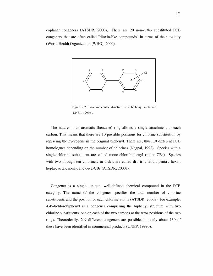
Fig. 2.2 shows the basic structure of a biphenyl molecule where the numbers 2-6
and 2’-6’ represent possible substitution locations for chlorine. Positions 2, 2', 6, and
6' are called ortho positions, positions 3, 3', 5, and 5' are called meta positions, and
positions 4 and 4' are called para positions. The benzene rings can rotate around the
bond connecting them. Their two extreme configurations are planar (i.e. two benzene
rings in the same plane) and non-planar (the benzene rings are at a 90° angle to each
other). The benzene rings of non-ortho substituted PCBs, as well as mono-ortho
substituted PCBs, may assume a planar configuration, referred to as planar or
17
coplanar congeners (ATSDR, 2000a). There are 20 non-ortho substituted PCB
congeners that are often called "dioxin-like compounds" in terms of their toxicity
(World Health Organization [WHO], 2000).
Figure 2.2 Basic molecular structure of a biphenyl molecule
(UNEP, 1999b).
The nature of an aromatic (benzene) ring allows a single attachment to each
carbon. This means that there are 10 possible positions for chlorine substitution by
replacing the hydrogens in the original biphenyl. There are, thus, 10 different PCB
homologues depending on the number of chlorines (Nagpal, 1992). Species with a
single chlorine substituent are called mono-chlorobiphenyl (mono-CBs). Species
with two through ten chlorines, in order, are called di-, tri-, tetra-, penta-, hexa-,
hepta-, octa-, nona-, and deca-CBs (ATSDR, 2000a).
Congener is a single, unique, well-defined chemical compound in the PCB
category. The name of the congener specifies the total number of chlorine
substituents and the position of each chlorine atoms (ATSDR, 2000a). For example,
4,4'-dichlorobiphenyl is a congener comprising the biphenyl structure with two
chlorine substituents, one on each of the two carbons at the para positions of the two
rings. Theoretically, 209 different congeners are possible, but only about 130 of
these have been identified in commercial products (UNEP, 1999b).
2 3
4
5 6
2' 3'
4'
5'
6'
Cl
X

18
18
Table 2.2 Selected physical-chemical properties of PCB congeners (1/2).
PCBs Cas-Noa Molecular Formulaa
Molecular Structurea
MWa
(g mol-1) TM
a (°C)
TBa
(°C) SW
b (25°C) (mg L-1)
VPb (25°C) (mm Hg)
Hc (at 25°C) (atm m3 mol-1)
log KOAd
(at 20°C) log KOWg
PCB-18 37680-65-2 C12H7Cl3 2,2',5 258 101 341 0.4 1.05E-03 2.52E-04 7.79 5.19
PCB-17 37680-66-3 C12H7Cl3 2,2',4 258 101 341 0.0833 4.00E-05 6.02E-04 7.74 5.33
PCB-31 16606-02-3 C12H7Cl3 2,4',5 258 101 341 0.143 4.00E-04 2.68E-04 8.4 5.66
PCB-28 7012-37-5 C12H7Cl3 2,4,4' 258 101 341 0.27 1.95E-04 3.63E-04 8.4 5.63
PCB-33 38444-86-9 C12H7Cl3 2',3,4 258 101 341 0.133* 1.03E-04 5.97E-04 8.52 5.46h
PCB-52 35693-99-3 C12H6Cl4 2,2',5,5' 292 122 360 0.0153 8.45E-06 3.11E-04 8.49 5.74
PCB-49 41464-40-8 C12H6Cl4 2,2',4,5' 292 122 360 0.0781* 8.48E-06 4.17E-04 8.63 5.91
PCB-44 41464-39-5 C12H6Cl4 2,2',3,5' 292 122 360 0.10* 8.45E-06 2.68E-04 8.71 5.62
PCB-74 32690-93-0 C12H6Cl4 2,4,4',5 292 122 360 0.00496 8.45E-06 4.17E-04 9.14 6.2
PCB-70 32598-11-1 C12H6Cl4 2,3',4',5 292 122 360 0.041 4.08E-05 2.77E-04 9.22 6.2
PCB-95 38379-99-6 C12H5Cl5 2,2',3,5',6 326 135 378 0.0211* 2.22E-06 6.29E-04 9.06 6.15
PCB-101 37680-73-2 C12H5Cl5 2,2',4,5,5' 326 135 378 0.0154 2.52E-05 4.29E-04 9.28 6.26
PCB-99 38380-01-7 C12H5Cl5 2,2',4,4',5 326 135 378 0.00366 2.20E-05 4.27E-04 9.38f 6.4
PCB-87 38380-02-8 C12H5Cl5 2,2',3,4,5' 326 135 378 0.0294* 1.70E-05 3.63E-04 9.25f 6.12
PCB-110 38380-03-9 C12H5Cl5 2,3,3',4',6 326 135 378 0.00731 2.22E-06 3.99E-04 9.58 6.22
PCB-82 52663-62-4 C12H5Cl5 2,2',3,3',4 326 135 378 0.0291* 2.22E-06 5.97E-04 9.16f 6.11
PCB-151 52663-63-5 C12H4Cl6 2,2',3,5,5',6 361 146 397 0.0136* 2.29E-06 1.35E-03 9.58 6.57
PCB-149 38380-04-0 C12H4Cl6 2,2',3,4',5',6 361 146 397 0.00424 8.43E-06 3.96E-04 9.74 6.46
PCB-118 31508-00-6 C12H5Cl5 2,3',4,4',5 326 135 378 0.0134* 8.97E-06 3.62E-04 10.04 6.72
PCB-153 35065-27-1 C12H4Cl6 2,2',4,4',5,5' 361 146 397 0.00095** 3.43E-06 5.40E-04 9.99 6.76
PCB-132 38380-05-1 C12H4Cl6 2,2',3,3',4,6' 361 146 397 0.00808 5.81E-07 2.83E-04 10.07 6.42
PCB-105 32598-14-4 C12H5Cl5 2,3,3',4,4' 326 135 378 0.0034 6.53E-06 3.39E-04 10.20 6.59
PCB-138 35065-28-2 C12H4Cl6 2,2',3,4,4',5' 361 146 397 0.0015* 3.80E-06 4.55E-04 10.20 6.68
PCB-158 74472-42-7 C12H4Cl6 2,3,3',4,4',6 361 146, 107b 397 0.00807* 1.55E-06a 8.11E-04 10.14 6.74
PCB-187 52663-68-0 C12H3Cl7 2,2',3,4',5,5',6 395 164 416 0.00451* 1.30E-07 6.64E-04 10.22 7.04
19
19
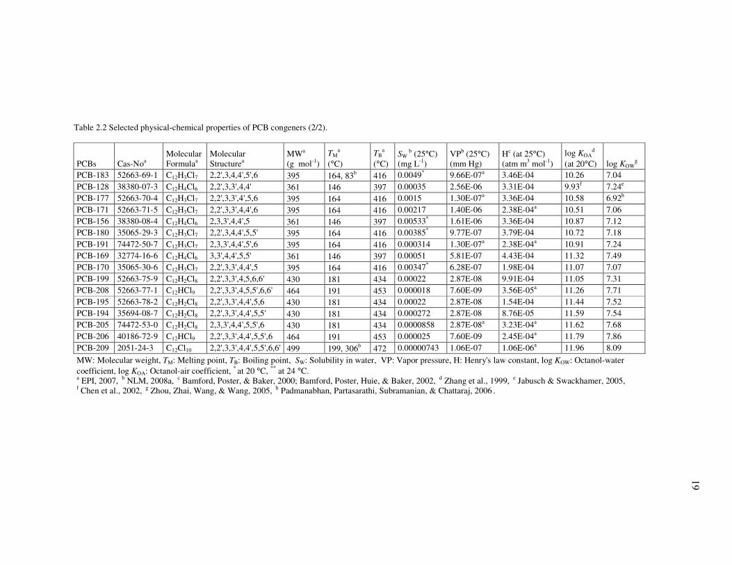
Table 2.2 Selected physical-chemical properties of PCB congeners (2/2).
PCBs Cas-Noa Molecular Formulaa
Molecular Structurea
MWa
(g mol-1) TM
a (°C)
TBa
(°C) SW
b (25°C) (mg L-1)
VPb (25°C) (mm Hg)
Hc (at 25°C) (atm m3 mol-1)
log KOAd
(at 20°C) log KOWg
PCB-183 52663-69-1 C12H3Cl7 2,2',3,4,4',5',6 395 164, 83b 416 0.0049* 9.66E-07a 3.46E-04 10.26 7.04
PCB-128 38380-07-3 C12H4Cl6 2,2',3,3',4,4' 361 146 397 0.00035 2.56E-06 3.31E-04 9.93f 7.24e
PCB-177 52663-70-4 C12H3Cl7 2,2',3,3',4',5,6 395 164 416 0.0015 1.30E-07a 3.36E-04 10.58 6.92h
PCB-171 52663-71-5 C12H3Cl7 2,2',3,3',4,4',6 395 164 416 0.00217 1.40E-06 2.38E-04a 10.51 7.06
PCB-156 38380-08-4 C12H4Cl6 2,3,3',4,4',5 361 146 397 0.00533* 1.61E-06 3.36E-04 10.87 7.12
PCB-180 35065-29-3 C12H3Cl7 2,2',3,4,4',5,5' 395 164 416 0.00385* 9.77E-07 3.79E-04 10.72 7.18
PCB-191 74472-50-7 C12H3Cl7 2,3,3',4,4',5',6 395 164 416 0.000314 1.30E-07a 2.38E-04a 10.91 7.24
PCB-169 32774-16-6 C12H4Cl6 3,3',4,4',5,5' 361 146 397 0.00051 5.81E-07 4.43E-04 11.32 7.49
PCB-170 35065-30-6 C12H3Cl7 2,2',3,3',4,4',5 395 164 416 0.00347* 6.28E-07 1.98E-04 11.07 7.07
PCB-199 52663-75-9 C12H2Cl8 2,2',3,3',4,5,6,6' 430 181 434 0.00022 2.87E-08 9.91E-04 11.05 7.31
PCB-208 52663-77-1 C12HCl9 2,2',3,3',4,5,5',6,6' 464 191 453 0.000018 7.60E-09 3.56E-05a 11.26 7.71
PCB-195 52663-78-2 C12H2Cl8 2,2',3,3',4,4',5,6 430 181 434 0.00022 2.87E-08 1.54E-04 11.44 7.52
PCB-194 35694-08-7 C12H2Cl8 2,2',3,3',4,4',5,5' 430 181 434 0.000272 2.87E-08 8.76E-05 11.59 7.54
PCB-205 74472-53-0 C12H2Cl8 2,3,3',4,4',5,5',6 430 181 434 0.0000858 2.87E-08a 3.23E-04a 11.62 7.68
PCB-206 40186-72-9 C12HCl9 2,2',3,3',4,4',5,5',6 464 191 453 0.000025 7.60E-09 2.45E-04a 11.79 7.86
PCB-209 2051-24-3 C12Cl10 2,2',3,3',4,4',5,5',6,6' 499 199, 306b 472 0.00000743 1.06E-07 1.06E-06a 11.96 8.09
MW: Molecular weight, TM: Melting point, TB: Boiling point, SW: Solubility in water, VP: Vapor pressure, H: Henry's law constant, log KOW: Octanol-water coefficient, log KOA: Octanol-air coefficient, * at 20 °C, ** at 24 °C. a EPI, 2007, b NLM, 2008a, c Bamford, Poster, & Baker, 2000; Bamford, Poster, Huie, & Baker, 2002, d Zhang et al., 1999, e Jabusch & Swackhamer, 2005, f Chen et al., 2002, g Zhou, Zhai, Wang, & Wang, 2005, h Padmanabhan, Partasarathi, Subramanian, & Chattaraj, 2006 .

20
Table 2.2 shows some physical-chemical properties of the studied PCB congeners
that vary widely depending on the degree of chlorination and the position of chlorine
atom on the biphenyl molecule. Although most PCB congeners are solids at room
temperature, the commercial mixtures are mobile oils, viscous fluids, or sticky resins
(Nagpal, 1992). Pure individual PCB congeners are colorless to light yellow and
have no known smell or taste (ATSDR, 2000a). They have extremely high boiling
points and are practically nonflammable. The important characteristics of PCBs that
have led to their widespread use are (i) thermal stability, (ii) high degree of chemical
stability, (iii) resistance to oxidation, acids, bases, and other chemical agents, and
(iv) excellent dielectric properties (i.e. low electrical conductivity) (UNEP, 1999b).
PCBs exhibit low vapor pressure (Nagpal, 1992) and their vapor pressures and
Henry’s law constants tend to decrease with increased chlorination. Thus, the more
chlorinated congeners are relatively non-volatile. PCBs with vapor pressures >10-4
mm Hg (mono- and di-CBs) appear to exist in the atmosphere almost entirely in the
gas-phase, while PCBs with vapor pressures <10-8 mm Hg appear to exist almost
entirely in the particle-phase, and PCBs with vapor pressures between 10-4 and 10-8
mm Hg (tri- to hepta-CBs) exist in both phases (ATSDR, 2000a).
PCBs are non-polar compounds. Their non-polar nature makes them only slightly
soluble in water, but they dissolve easily in fats, oils, and most organic solvents
(UNEP, 1999b). Generally, water solubility of PCBs decreases as the degree of
chlorine substitution increases. Within a homologue group, the solubility depends on
the positions of the chlorine atoms on the biphenyl ring (Nagpal, 1992).
PCBs are often associated with the solid fraction (e.g. particulate matter,
sediment, soil) of the aquatic and terrestrial environments. In general, sorption
tendency of PCBs increases with increasing degree of chlorination, the surface area
and the organic carbon content of the sorbents (Nagpal, 1992). The higher
chlorinated PCBs with lower water solubility and higher KOW values have a greater
tendency to bind to solids as a result of strong hydrophobic interactions. In contrast,

21
the low molecular weight PCBs with higher water solubility and lower KOW values
sorb to a lesser extent on solids and remain largely in the aquatic environments.
Therefore, in comparison with the lower chlorinated PCBs, volatilization of highly
chlorinated ones in the aquatic and terrestrial environments is reduced significantly
by binding these compounds to solids (ATSDR, 2000a).
Most PCB congeners are extremely persistent in the environment. They are
estimated to have half-lives ranging from three weeks to two years in air and more
than six years in aerobic soils and sediments, with the exception of mono- and di-
chlorobiphenyls (UNEP, 2002). Due to their stability and lipophilicity, PCBs bio-
accumulate in food chains and are stored in fatty tissues of exposed animals and
humans (ATSDR, 2000a).
In people, some acute (e.g. skin conditions, spasms, hearing and vision problems)
and chronic (e.g. irritation of nose and lungs, gastrointestinal discomfort, changes in
blood and liver, depression, fatigue, and possibly cancer) adverse health effects have
been linked to PCBs. The U.S. EPA and the IARC have determined that certain PCB
mixtures including Araclor-1016, -1242, -1254 and -1260 are probably carcinogenic
(Group B2) to humans (U.S. EPA, 2002b).
2.2.2 Production and Uses of PCBs
PCBs are synthetic chemical compounds and their production involves the
chlorination of biphenyl in the presence of a catalyst. Depending on the reaction
conditions, the degree of chlorination varies between 21 and 68% chlorine on a
weight-by-weight basis (Breivik, Sweetman, Pacyna, & Jones, 2002a).
Commercially produced PCBs are a complex mixture of individual PCB congeners,
and they were marketed under several trade names including Aroclor, Askarel,
Pyroclor, Santotherm, Kennechlor, Hyvol, Chlorextol, and Pyranol (Nagpal, 1992).
The most common trade name is Aroclor.

22
There are many types of Aroclors and each of them is characterized by a four digit
number that indicates the degree of chlorination. The first two digits generally refer
to the number of carbon atoms in the phenyl rings. For PCBs, this is 12. The last two
digits indicate the percentage of chlorine by mass in the mixture. For example, the
name Aroclor 1254 means that the mixture contains approximately 54% chlorine by
weight. Therefore, higher Aroclor numbers reflect higher chlorine content (ATSDR,
2000a; UNEP, 1999b).
The industrial and commercial uses of PCBs (ATSDR, 2000a; Breivik,
Sweetman, Pacnya, & Jones, 2002b; U.S. EPA & Oregon Department of
Environmental Quality [DEQ] 2005; UNEP, 1999b; Vallack et al., 1998) can be
classified based on their presence in closed, partially closed, and open systems as
follows:
• Closed system applications (as coolants and dielectric fluids in transformers,
capacitors, electric motors, and electrical household appliances such as
television sets, refrigerators, air conditioners, microwave ovens; in
fluorescent light ballast, and electromagnets),
• Partially closed system applications (as heat transfer fluids in mechanical
operations at the inorganic/organic chemicals, plastics and synthetics, and
petroleum refining industries; as hydraulic fluids in mining equipment,
aluminum, copper, steel, and iron forming industries; in gas turbines and
vacuum pumps; in electrical equipment such as voltage regulators, switches,
circuit breakers; as stabilizing additives in flexible PVC coatings of electrical
wiring and electronic components, in cable insulation materials), and
• Open system applications (as ink solvents in carbonless copy paper; as
plasticizers in polyvinyl chloride (PVC) plastics, rubber, synthetic resins, and
sealants; as additives in cement and plaster; in casting waxes; in paints,
textiles, surface coatings, de-dusting agents, asphalt, natural gas pipelines,
flame retardants; adhesives; in insulating materials; pesticide extenders; in
lubricating and cutting oils; in dyes and printing inks).

23
Products such as oil, carbonless copy paper and plastics made with recycled PCB
materials, and automobiles with PCB containing oil, fluids and cables have been also
reported (UNEP, 1999b; U.S. EPA & DEQ, 2005).
The production and use of PCBs have been banned for decades in many countries.
In Turkey, the uses of PCBs were banned in 1995, except for the closed system uses
such as capacitors and transformers that are already in-use (Acara et al., 2006).
2.2.3 Sources of PCBs
Generally, closed and partially closed systems contain PCB oils and fluids. PCBs
in closed systems can not readily escape into the environment. However, they may
be released during equipment servicing, repairing, or as a result of damaged
equipment. Also, the reclamation process for used out instruments and wasted
material is a possible source. PCBs in partially closed systems are not directly
exposed to the environment, but may be released periodically during typical use or
discharge. The PCBs in open systems take on the form of the product used in as a
component. Open systems are applications in which PCBs are in direct contact with
their surroundings and thereby, they may be easily transferred to the environment
(UNEP, 1999b).
Because their hazardous nature has only recently been understood, PCBs have
been routinely disposed of over the years without any precautions being taken. As a
result, large volumes of PCBs have been released into the environment from illegal
or improper dumping of PCB wastes into landfills; open burning; incineration of
industrial and municipal wastes (e.g. refuse, sewage sludge, products containing
PCBs); vaporization from contaminated surfaces and products containing PCBs;
accidental spills and leakage from products to soils; direct entry or leakage into
sewers and streams; leakage from older electrical equipment in use; the repair and
maintenance of PCB containing equipment (Breivik et al., 2002b; UNEP, 1999b;
U.S. EPA & DEQ, 2005; Vallack et al., 1998).

24
Recycling operations of PCB containing materials (e.g. oil, carbonless copy
paper, PVC plastic, and scrap metal) are the other PCB source to the environment. In
scrap metal recycling operation, PCBs are emitted from transformer shell salvaging;
heat transfer and hydraulic equipment; and shredding and smelting of waste
materials such as cars, electrical household appliances (e.g. refrigerators, air
conditioners, television sets, and microwave ovens) and other appliances used for
upholstery, padding, and insulation. In iron-steel industries, PCBs are also released
from non-ferrous metal salvaging as parts from PCB containing electrical equipment,
and oil/grease insulated electrical cable (UNEP, 1999b; U.S. EPA & DEQ, 2005).
PCBs emissions may be generated from various thermal processes in the
production of organic pigments, pesticides, chemicals (such as PVC manufacturing
and petroleum refining industries), cement, copper, iron-steel, and aluminum refining
industries. In these processes, they may be synthesized like dioxins. The forming of
PCBs as a by-product is possible when chlorine, hydrocarbon and elevated
temperatures together with catalysts (UNEP, 1999b).
PCBs are combustible liquids, and the products of combustion may be more
hazardous than the original material. Combustion by-products include hydrogen
chloride, polychlorinated dibenzodioxins/dibenzofurans (PCDD/DFs). The pyrolysis
of commercial PCB mixtures produces several PCDFs. PCDFs are also produced as
a by-product during the commercial production and handling of PCBs, and as
impurities in various commercial PCB mixtures (ATSDR, 2000a).
2.3 Organochlorine Pesticides (OCPs)
Organochlorine pesticides (OCPs) are mostly used as insecticides in agriculture.
Some OCPs have been banned for decades in many countries because of concerns
about environmental and human health impacts (Acara et al., 2006). However,
banned OCPs are still found in the environment, probably due to their persistence,
illegal uses or emissions from certain industrial sources. OCPs restricted/banned or

25
remained in-use are mainly released to the atmosphere by agricultural usage,
volatilization from contaminated soil, and particulate matter re-entrainment from the
surface cover by the wind at contaminated areas (Bidleman, 1999).
Once released, OCPs can be partitioned to all environmental matrices such as air,
water, soil, and sediment. Due to their semi-volatile nature, they can exist in the
atmosphere as a gas and/or attached to airborne particles, and can be transported over
long distances. Although their atmospheric lifetime is long, they can be degraded by
reacting with photo-chemically produced hydroxyl radicals or can be removed from
the air by wet and dry deposition (ATSDR, 2005).
OCPs are generally stable in the environmental matrices and undergo limited
decomposition and/or degradation. In soil, sediment, and water, they are broken
down to less toxic substances by algae, fungi, and bacteria, but this process can take
a long time. Biodegradation is believed to be the dominant decomposition process
for OCPs in soil and water, although hydrolysis and photolysis may also occur to a
lesser extent. The rates of degradation processes depend on the ambient
environmental conditions. Since most OCPs are bio-accumulative, they build up in
the food chain as well as in fatty tissues of animals and humans (ATSDR, 2005;
Regional Water Quality Control Plant [RWQCP], 1997).
2.3.1 Chemical Structures, Properties, and Health Effects of OCPs
Organochlorine pesticides vary in their chemical structures and mechanisms of
toxicity. Subcategories of this group include dichlorodiphenylethanes (e.g. DDT,
methoxychlor, dicofol, chlorobenzilate); cyclodienes (e.g. aldrin, dieldrin, endrin,
chlordane, heptachlor, endosulfan, mirex); chlorinated benzenes (e.g.
hexachlorobenzene [HCB]); and cyclohexanes (e.g. hexachlorocyclohexane [HCH],
lindane) (U.S. EPA, 2002a, 2002b; WHO, 1979). In this study, chlorpyrifos is the
only studied compound that belongs to the group of organophosphate insecticide.

26
Chemical structures of some pesticides and their degradation products are
illustrated in Fig. 2.3, and selected physical-chemical properties of studied pesticides
are given in Table 2.3. In this section, studied pesticides were evaluated according to
their related groups and metabolites. The structures and many physical-chemical
properties of related pesticides are very similar. For example, cyclodiene pesticides
are a large group of highly chlorinated cyclic hydrocarbons with characteristic
endomethylene bridged structures. They are highly persistent compounds, exhibiting
especially high resistance to degradation in soil (U.S. EPA, 2002a). DDT related
pesticides have a different type of structure, but they also share some properties with
other OCPs such as chlordane, dieldrin, and heptachlor (RWQCP, 1997).
2.3.1.1 Hexachlorocylclohexane (HCH)
Hexachlorocylclohexane (HCH) is an organochlorine insecticide consisting of
eight isomers. But, only alpha- (α), beta- (β), gamma- (γ), and delta- (δ) isomers are
of commercial significance. Different isomers are named according to the position of
the hydrogen atoms in the structure. Pure γ-HCH, commonly called lindane, is the
only isomer with insecticidal activity. Technical HCH mixture is comprised of
approximately 60-70% α-HCH, 5-12% β-HCH, 10-15% γ-HCH, 6-10% δ-HCH, and
other isomers. HCHs are brownish- to white-colored crystalline solids or fine plates
with a phosgene-like odor (ATSDR, 2005).
γ-HCH can be released into the atmosphere both as lindane and as a component of
technical HCH. Agricultural application of lindane constitutes the largest source of γ-
HCH to the environment. α-HCH has the highest proportion in technical HCH
mixtures, and it can be released into the atmosphere only as a component of technical
HCH. The main degradation of HCH isomers in the air occurs through the
photochemical reaction with hydroxyl radicals (ATSDR, 2005).

27
HCHs α-HCH β-HCH γ-HCH (Lindane) δ-HCH
Chlorpyrifos
Cyclodienes
(Heptachlor,
Chlordane and
metabolites)
Heptachlor Heptachlor epoxide α-Chlordane
γ-Chlordane c-Nonachlor t-Nonachlor
(Endosulfan
and
metabolites)
Endosulfan-I (α-Endosulfan) Endosulfan -II (β-Endosulfan) Endosulfan sulfate

28
(Aldrin
Dieldrin)
Aldrin Dieldrin
(Endrin and
metabolites)
Endrin Endrin aldehyde Endrin ketone
DDT related
pesticides
(DDT and
metabolites,
methoxychlor)
p,p'-DDT p,p'-DDD p,p'-DDE Methoxychlor
Figure 2.3 Chemical structures of the some related pesticides and their metabolites (NLM, 2008a).

29
29
Table 2.3 Selected physical-chemical properties of the studied pesticides.
OCPs** CAS-Noa Molecular Formulaa
MWa (g mol-1) TM
b (°C) TBb (°C)
SW a (25oC)
(mg L-1) VPa (25oC) (mm Hg )
Hc (25oC) (atm m3 mol-1)
log KOAe
(25oC) log KOWa
α-HCH 319-84-6 C6H6Cl6 291 57, 160a 304, 288a 2.0 4.50E-05 2.96E-06 7.61 3.80
β-HCH 319-85-7 C6H6Cl6 291 57, 315a 304 0.24 3.60E-07* 3.55E-07d 8.88 3.78
γ-HCH 58-89-9 C6H6Cl6 291 57, 113a 304, 323a 7.3 4.20E-05* 2.66E-06 7.85 3.72
δ-HCH 319-86-8 C6H6Cl6 291 57, 142a 304 10.0* 3.52E-05 4.29E-07a 8.84 4.14
CHLPYR 2921-88-2 C9H11Cl3NO3PS 351 83, 42a 377 1.12** 2.03E-05 3.55E-05 8.41f 4.96
HEP EPOX 1024-57-3 C10H5Cl7O 389 133, 160a 341 0.20 1.95E-05*** 2.27E-05 8.50f 4.98
α-CHL 5103-71-9 C10H6Cl8 410 133 351 0.056 3.60E-05 5.43E-05 8.92 6.10
γ-CHL 5103-74-2 C10H6Cl8 410 133 351 0.056 5.03E-05 1.57E-04 8.87 6.22
c-NONA 5103-73-1 C10H5Cl9 444 148 372 0.0104 9.00E-07 5.92E-06 9.66 6.08
t-NONA 39765-80-5 C10H5Cl9 444 148 372 0.0104 1.00E-06 1.06E-04 9.29 6.35
ESLF-I 959-98-8 C9H6Cl6O3S 407 166 401 0.51* 3.00E-06 8.09E-06 8.64 3.83
ESLF-II 33213-65-9 C9H6Cl6O3S 407 166 401 0.45* 6.00E-07 6.51E-07 9.28f 3.83
ESULFATE 1031-07-8 C9H6Cl6O4S 423 170, 181-182a 409 0.48* 2.80E-07 3.25E-07a 9.68f 3.66
p,p'-DDT 50-29-3 C14H9Cl5 354 123, 109a 368 0.0055 1.6E-07* 9.57E-06 9.82 6.91
p,p'-DDD 72-54-8 C14H10Cl4 320 114, 110a 367, 350a 0.09 1.35E-06 9.47E-06 10.10 6.02
DIELD 60-57-1 C12H8Cl6O 381 135, 176a 340, 330a 0.195 5.89E-06 9.77E-06 8.90 5.40
END 72-20-8 C12H8Cl6O 381 135, 226-230a 340 0.25 3.00E-06* 5.62E-06 8.13 5.20
END AL 7421-93-4 C12H8Cl6O 381 138 340 0.024 2.00E-07 4.18E-06a 9.47f 4.80
END KET 53494-70-5 C12H8Cl6O 381 146 357 0.222 5.51E-06 2.02E-08a 10.11f 4.99
MEOCL 72-43-5 C16H15Cl3O2 346 129, 87a 378, 346a 0.10 2.58E-06 2.03E-07a 10.57f 5.08 ** α,β,γ,δ-Hexachlorocyclohexane isomers (α,β,γ,δ-HCH), chlorpyrifos (CHLPYR), heptachlor epoxide (HEP EPOX), α-chlordane (α-CHL), γ-chlordane (γ-CHL), cis-nonachlor (c-NONA), trans-nonachlor (t-NONA), endosulfan-I (ESLF-I), endosulfan-II (ESLF-II), endosulfan sulfate (ESLF SUL), dichlorodiphenyl trichloroethane (p,p'-DDT), tetrachlorodiphenylethane (p,p'-DDD), dieldrin (DIELD), endrin (END), endrin aldehyde (END AL), endrin ketone (END KET), methoxychlor (MEOCL). MW: Molecular weight, TM: Melting point, TB: Boiling point, SW: Solubility in water, VP: Vapor pressure, H: Henry's law constant, log KOA: Octanol-air coefficient, log KOW: Octanol-water coefficient, * at 20 °C, ** at 24 °C, *** at 30 °C. a NLM, 2008a, b EPI, 2007, c Cetin, Ozer, Sofuoglu, & Odabasi, 2006, d Sahsuvar, Helm, Jantunen, & Bidleman, 2003, e Shoeib & Harner, 2002, f Odabasi , 2007a.

30
Among HCH isomers, α- and γ-HCH are more ubiquitous in the environment.
Although both isomers have relatively high vapor pressures, γ-HCH has a higher
value than that of α-HCH (Gioia et al., 2005). Thus, atmospheric lindane
concentrations tend to be more strongly correlated with temperature and more
influenced by volatilization from terrestrial surfaces. However, global atmospheric
background concentrations are higher for α-HCH than γ-HCH possibly because α-
HCH is more persistent (Wania, Haugen, Lei, & Mackay, 1998).
The occurrence of HCH isomers in water supplies is more important potential
problem than many other OCPs (e.g. DDT, endrin, aldrin, heptachlor) due to their
high water solubility. γ-HCH has a low residence time in the aquatic environment
and the principal dissipation routes are sedimentation, biodegradation, and
volatilization. Thus, γ-HCH is generally found to contribute less to aquatic pollution
than the other HCH isomers (U.S. EPA, 1980a).
HCHs are much less bio-accumulative than other OCPs because of their relatively
low liphophilic properties. Lindane and other HCH isomers are relatively persistent
in soils and water, with half-lives generally greater than 1 and 2 years, respectively
(UNEP, 2002). HCHs in soil or sediment are degraded primarily by biodegradation.
The biological transformation of HCHs results in the formation of various
cyclophenols including 2,3,5-, 2,4,5- and 2,4,6-trichlorophenol; 3,4-dichlorophenol;
2,3,4,5- and 2,3,4,6-tetrachlorophenol (U.S. EPA, 1980a). γ-HCH is also transformed
to tetrachlorohexene; tri-, tetra-, and penta-chlorinated benzenes; penta- and tetra-
cyclohexanes; and other isomers of HCH (ATSDR, 2005).
Several hepatic, immunological, hematological, neurological, reproductive, and
carcinogenic effects have been reported in humans exposed to HCHs. Among HCH
isomers, γ-HCH (lindane) has the highest acute toxicity (U.S. EPA, 1980a). The
World Health Organization (WHO) has determined that HCH and lindane are
classified as Class II, moderately hazardous chemicals (WHO, 2005). The IARC has
classified all HCH isomers as possibly carcinogenic to humans. The U.S. EPA has
31
determined technical HCH and α-HCH as Group B2, probable human carcinogens,
and β-HCH as Group C, possible human carcinogen. The U.S. EPA has also
classified lindane as having “suggestive evidence of carcinogenicity, but not
sufficient to assess its human carcinogenic potential” (ATSDR, 2005).
2.3.1.2 Chlorpyrifos
Chlorpyrifos, also known as chlorpyrifos ethyl, is an organophosphate pesticide.
However it is rather unusual in this group, since it has a high degree of chlorination.
This chlorination gives certain properties that are not typically noted for this general
class of compounds. The important properties are its low water solubility, more lipid
solubility, and adsorption tendency to particulate matter, soil or sediment. These
properties make it more persistent than most other pesticides in this general group
(U.S. EPA, 2002b).
Chlorpyrifos is a white crystalline solid that has a strong odor (U.S. EPA, 2002b).
Chemical hydrolysis, photo-degradation, and biodegradation are all important
processes for the transformation and degradation of chlorpyrifos (Miller, 1996).
Because of its low water solubility and its affinity for organics, it has little mobility
in most soils. When chlorpyrifos enters an aquatic system, it appears to be sorbed
readily to suspended organics and sediment, although some is removed by
volatilization and degradation. Its penetration into sediment appears to be shallow,
with most occurring in the upper layers. Although chlorpyrifos is hydrophobic, it
bio-concentrates or accumulate in living tissues to only a limited extent because of
its rapid metabolism (ATSDR, 1997; U.S. EPA, 1986). 3,5,6-trichloro-2-pyridinol
(TCP) is a major metabolite of this compound (ATSDR, 1997).
In people, short-term oral exposure to low levels of chlorpyrifos can cause
dizziness, fatigue, runny nose or eyes, salivation, nausea, intestinal discomfort,
sweating, and changes in heart rate. Much higher levels of chlorpyrifos may cause
paralysis, seizures, loss of consciousness, and death. Other effects of exposure to

32
chlorpyrifos include changes in behavior or sleeping pattern, mood changes, and
effects on the nerves and/or muscles in the limbs, which may appear as odd
sensations such as numbness, tingling, or muscle weakness. Chlorpyrifos is classified
as Class II, moderately hazardous chemical by WHO (2005). The U.S. EPA has not
classified chlorpyrifos for carcinogenicity (Class D) (ATSDR, 1997).
2.3.1.3 Heptachlor
Heptachlor is a cyclodiene insecticide that has a chemical structure and
mechanism of toxicity similar to that of chlordane. It is also both a breakdown
product and a minor component of chlordane (U.S. EPA, 2002b). Pure heptachlor is
a white powder that does not burn easily and does not explode. Technical product is
a tan powder and usually consists of 72% heptachlor and 28% impurities such as
trans-chlordane, cis-chlordane, and nonachlor (ATSDR, 2007).
Heptachlor epoxide is an oxidation breakdown product of heptachlor and
chlordane. It degrades more slowly, and thus, it is more persistent in the environment
than heptachlor. Heptachlor epoxide is also considered more toxic than its parent
compound. Although both of them do not dissolve easily in water, heptachlor
epoxide dissolves more easily in water than heptachlor does (ATSDR, 2007)
Both heptachlor and heptachlor epoxide have relatively high log KOC values that
suggest a high sorption tendency. This means that these compounds are not mobile in
soil and have a low potential to leach. However, they have some volatilization
potential from the contaminated surfaces to the air (Miller, 1996). The half-life of
heptachlor in soil is 0.75-2 years in temperate regions (UNEP, 2002). Based on their
high partition coefficient, both are bio-concentrated in aquatic and terrestrial
organisms. Because of its lipophilicity and its more persistent nature, bio-
magnification of heptachlor epoxide in food chain is significant (ATSDR, 2007).
33
In humans, heptachlor results in a variety of adverse health effects including liver
effects, neurological effects, reproductive system dysfunction, and developmental
effects. The U.S. EPA and the IARC have classified heptachlor as a possible human
carcinogen. The U.S. EPA also considers heptachlor epoxide as a possible human
carcinogen (ATSDR, 2007).
2.3.1.4 Chlordane
Chlordane belongs to the cyclodiene group of insecticides, and it is structurally
quite similar to heptachlor and heptachlor epoxide. Technical chlordane is a mixture
of various related chemicals with a typical composition of ~15% cis- (or α-)
chlordane, 15% of trans- (or γ-) chlordane, 9.7% of trans-nonachlor, 3.9% octa-
chlordane, 3.8% heptachlor, 2.7% cis-nonachlor and other compounds. The
composition of technical chlordane varies according to conditions during its
manufacture (U.S. EPA, 1997).
Chlordane is a thick liquid whose color ranges from colorless to amber,
depending on its purity. It may have no smell or a mild, irritating smell. The
physical-chemical properties of technical chlordane are difficult to specify, since the
technical product is a mixture of over 140 compounds. Properties of a mixture also
differ from the properties of the components. Compositional changes with time may
result from different rates of degradation and transport among the constituents of the
mixture (ATSDR, 1994).
Generally, chlordane and related compounds are insoluble in water, but soluble in
fat and bio-concentrate in fatty tissues. Especially cis- and trans-chlordane have high
Henry’s law coefficients which make them more volatile than other pesticides (Table
2.3). Combined with their persistence in the environment, they are likely to undergo
long-range transport (U.S. EPA, 2002b).

34
In the environment, chlordane is metabolized to oxy-chlordane and heptachlor.
Heptachlor is also metabolized to heptachlor epoxide as described above. Chlordane
is an unlikely source of exposure if heptachlor epoxide is found in the absence of
either oxy-chlordane or trans-nonachlor. The most persistent compounds in
biological tissue are oxy-chlordane and heptachlor epoxide which are of primary
toxicological significance (U.S. EPA, 1997).
Like most of the other cyclodiene pesticides, chlordane is highly immobile within
the soil, since it is both insoluble in water and rapidly binds to soil particles. It has a
half-life of about 4 years in soils depending on the environmental conditions (UNEP,
2002). Evaporation is the major route of removal from soils. Also, it has a low
potential for groundwater contamination (Miller, 1996; ATSDR, 1994).
Major health effects in humans that may be linked to chlordane exposure are on
the nervous system, the digestive system, and the liver. Large amounts of chlordane
taken by mouth can cause convulsions and death. Swallowing small amounts or
breathing air containing high concentrations of chlordane vapors can cause a variety
of nervous system effects, including headaches, irritation, confusion, weakness, and
vision problems, as well as upset stomach, vomiting, stomach cramps, diarrhea, and
jaundice (ATSDR, 1994). The WHO classified chlordane as Class II, moderately
hazardous (WHO, 2005). The IARC has determined that chlordane is not classifiable
as to its carcinogenicity to humans. However, the U.S. EPA lists chlordane in Group
B2, probable human carcinogen (ATSDR, 1994).
2.3.1.5 Endosulfan
Endosulfan belongs to the group of chlorinated cyclodiene insecticides (U.S.
EPA, 1980b). Technical endosulfan contains a mixture of its two different forms:
~70% of endosulfan-I (α-isomer) and 30% of endosulfan-II (β-isomer). Endosulfan is
a light to dark brown crystalline solid that does not burn. It has a distinct odor similar
to turpentine (ATSDR, 2000b).

35
Endosulfan sulfate is the main degradation product of endosulfan as a result of
oxidation, biotransformation or photolysis mechanisms (Hafner & Hites, 2003). Both
isomers of endosulfan are also metabolically converted by microorganisms, plants,
and animals to endosulfandiol, endosulfan ether, endosulfan hydroxyether, and
endosulfan lactone in the environment (U.S. EPA, 1980b). ATSDR (2000b) has
reported that the β-isomer (endosulfan-II) is also slowly converted to the more stable
α-isomer (endosulfan-I) at high temperatures.
In soil, endosulfan is most likely subjected to photolysis (on soil surfaces),
hydrolysis (under alkaline conditions), or biodegradation. Because of its very low
solubility, it does not easily dissolve in water. Based on the relationship between the
partition coefficients of KOW and KOC, endosulfan has a moderate capacity to adsorb
to soils and it is not likely to leach to groundwater. Thus, it is also moderately
persistent in the soil environment with a reported average field half-life of 50 days.
The α- and β-isomers have different degradation times in soil with half-lives of 35
and 150 days (in neutral conditions), respectively (UNEP, 2002). Due to their low
KOW values, endosulfan and metabolites do not bio-accumulate to high
concentrations in terrestrial or aquatic ecosystems (ATSDR, 2000b).
There is very little difference in toxicity between endosulfan and its metabolite,
endosulfan sulfate. However, the α-isomer has been shown to be about three times as
toxic as the β-isomer of endosulfan (ATSDR, 2000b). Exposure to very large
amounts of endosulfan for short periods can cause adverse effects on nervous system
such as hyper-excitability, tremors, convulsions, and dizziness. Chronic signs include
intermittent muscle twitching, psychological disorders, loss of consciousness, and
convulsions. In animal studies, long-term exposure to low levels of endosulfan has
been shown to affect the kidney, testes, and liver. Effects on the immune system, and
decreased weight gain were also noted (U.S. EPA, 2002b). The WHO classified
endosulfan as Class II, moderately hazardous substance (WHO, 2005). The IARC
and U.S. EPA have not classified endosulfan regarding its ability to cause cancer
(ATSDR, 2000b).

36
2.3.1.6 Aldrin and Dieldrin
Aldrin and dieldrin are structurally similar compounds that belong to cyclodiene
series of insecticides. Since aldrin is readily converted to dieldrin in the environment,
these two compounds are discussed together in this section. Technical aldrin contains
at least 85.5% aldrin, and technical dieldrin contains at least 85% dieldrin. Pure
aldrin and dieldrin are white powders, while technical-grade aldrin and dieldrin are
tan powders. Both insecticides have mild chemical odors (ATSDR, 2002b).
Aldrin is readily converted by natural processes into the more stable and
persistent compound of dieldrin. Thus, as a pesticide residue, aldrin is rarely detected
in its original chemical form into the environment (U.S. EPA, 2002b; RWQCP,
1997). Since dieldrin is more resistant to biotransformation and abiotic degradation,
it is found ubiquitously in all environmental media where aldrin and dieldrin were
originally released (ATSDR, 2002b).
Aldrin and dieldrin are non-polar compounds. Therefore, they have a strong
affinity for organic matter and sorbs tightly to soil particulates. Movement of dieldrin
through the soil column is extremely slow, indicating little potential for groundwater
contamination. Based on their physical properties, volatilization from soil or water
surfaces is expected, however, this may be decreased by adsorption to suspended
solids and sediment in the water column. Most aldrin and dieldrin found in surface
water are the result of runoff from contaminated soil (ATSDR, 2002b).
Aldrin undergoes photolysis to dieldrin which in turn may be degraded by
ultraviolet radiation or microbial action into the more persistent compound, photo
dieldrin (ATSDR, 2002b). Aldrin is classified as moderately persistent with half-life
in soil and surface waters ranging from 20 days to 1.6 years. Dieldrin is much more
resistant to biodegradation than aldrin. It is highly persistent in soils, with a half-life
of 3-4 years in temperate climates (UNEP, 2002). Both aldrin and dieldrin are bio-
concentrated by plants, animals, and aquatic organisms, and biomagnified in aquatic

37
and terrestrial food chains. Food chain bioaccumulation appears to be a more
important fate process for dieldrin than for aldrin, since aldrin is rapidly converted to
more stable form, dieldrin. Atmospheric aldrin and dieldrin compounds in gas-phase
are expected to react with hydroxyl radical. Gas-phase aldrin may also be degraded
in the air by reaction with ozone (ATSDR, 2002b). The persistence in air has been
estimated in 4-40 hrs (UNEP, 2002)
Aldrin and dieldrin affect human health in similar ways. Exposure to large
amount of both pesticides for short periods can cause convulsions or other nervous
system effects, and kidney damage. Some people who intentionally ate or drank
large amounts of aldrin or dieldrin died. In people exposed to smaller amounts of
aldrin or dieldrin, adverse health effects occur, because levels of the chemicals build
up in the body over time. Exposure to moderate levels of aldrin or dieldrin for a long
time causes headaches, dizziness, irritability, vomiting, or uncontrollable muscle
movements. They also can destroy the blood cells in human body. The IARC has
determined that aldrin and dieldrin are not classifiable as to their carcinogenicity to
humans. However, aldrin and dieldrin are both classified by the U.S. EPA as Group
2, probable human carcinogens (ATSDR, 2002b).
2.3.1.7 Endrin
Endrin is a stereoisomer of dieldrin, and a member of cyclodiene group of
pesticides (U.S. EPA, 2002b). Endrin is also a contaminant in dieldrin. Endrin
aldehyde and endrin ketone occurred as impurities of eldrin or as degradation
products. While technical-grade endrin is typically 95-98% pure, some chemicals are
found as impurities including aldrin, dieldrin, isodrin, heptachloronorbornadiene, and
heptachloronorborene in addition to endrin aldehyde and endrin ketone (ATSDR,
1996). Pure endrin is a white crystalline solid that is almost odorless, while the
technical compound is a light tan powder (U.S. EPA, 1980c).

38
Endrin is a highly persistent chemical in the environment, particularly in soils.
Because of its low solubility in water, leaching may be possible in some soils under
certain conditions. Half-lives of up to 12 years have been reported in some cases
(UNEP, 2002). Biodegradation and hydrolysis does not appear to be a significant
fate process for endrin in soils. In combination with losses from volatilization, photo-
degradation, and heat transformation (primarily to endrin ketone with minor amounts
of endrin aldehyde) account for the rapid decrease in endrin residues on soil surfaces
exposed to sunlight (ATSDR, 1996).
Endrin is the most acutely toxic compound among the cyclodiene group of
insecticides (U.S. EPA, 2002b). In humans, the primary toxic effect of acute
exposure to endrin is on the nervous system. Symptoms are headache, dizziness,
nervousness, confusion, nausea, vomiting, convulsions, hyper-excitability, and
seizures (ATSDR, 1996). Chronic signs of toxicity include intermittent muscle
twitching, psychological disorders, loss of consciousness, and convulsions (U.S.
EPA, 2002b). The U.S. EPA and the IARC have determined that endrin is not
classifiable for its human carcinogenety (ATSDR, 1996).
2.3.1.8 Dichlorodiphenyltrichloroethane (DDT)
Technical-grade DDT consists of different isomers with similar properties. Its
formulation mainly contains 65-80% of p,p'-DDT and other chemical forms of DDT
including o,o'-DDT, and o,p'-DDT. Isomers of p,p'-DDD and p,p'-DDE occurs as
impurities in technical DDT as well as its degradation product. Although both of the
degradation products are toxic, DDE is the more persistent and more toxic metabolite
of DDT (ATSDR 2002a).
Technical DDT is a white amorphous powder that is odorless or may have a slight
aromatic odor. It melts over the range of 80-94 °C. Pure p,p´-DDT is a colorless
crystalline solid or powder-like substance with weak aromatic odors. It is very
39
soluble in fats and most organic solvents, but insoluble in water. p,p´-DDT is a
flammable substance with a range of flash point 72-75 °C (UNEP, 2006).
Because of their semi-volatile nature, p,p'-DDT, p,p'-DDE, and p,p'-DDD are
found in the atmosphere both as gaseous or attached to airborne particulates, and
undergo long-range transport. Both p,p'-DDE and p,p'-DDD have higher vapor
pressures than p,p'-DDT, and thus, a smaller fraction of p,p'-DDE and p,p'-DDD are
adsorbed to particulate matter than p,p'-DDT (ATSDR, 2002a). Gas-phase p,p'-DDT
and its metabolites are subject to direct photo-degradation and reaction with photo-
chemically produced hydroxyl radicals (UNEP, 2006).
When deposited on soil, routes of loss and degradation include runoff,
volatilization, photolysis, and biodegradation. p,p'-DDT biodegrades primarily to
p,p'-DDE under un-flooded conditions (e.g. aerobic) and to p,p'-DDD under flooded
(e.g. anaerobic) conditions (ATSDR, 2002a). However, these processes generally
occur only very slowly. DDT is highly persistent in soils with a half-life of up to 15
years and of 7 days in air depending on conditions (UNEP, 2002). As a result of their
strong binding to soil (as reflected by their high KOC values), p,p'-DDT, p,p'-DDE,
and p,p'-DDT mostly remain on the surface layers of soil. They do not dissolve in
water, and are essentially immobile in soil. Thus, there is little leaching into the
lower soil layers and groundwater. As reflected by their high log KOW values (Table
2.3), p,p'-DDT and its degradation products adsorb strongly to particulate matter in
the water column and primarily partition into the sediment. But, some of them may
volatilize into the air. The persistence of DDT and its metabolites in combination
with their high lipophilicity have contributed to the bioaccumulation and bio-
magnification of these compounds in the environment (ATSDR, 2002a).
In humans, acute overdoses of DDT affect most likely the nervous system. People
who swallowed large amounts of DDT may become excitable and may have tremors
and seizures. Other symptoms are sweating, headache, nausea, vomiting, and
dizziness. The same types of effects are expected by breathing DDT particles in the
40
air or by contact of the skin with high amounts of DDT. People exposed for a long
time to small amounts of DDT have some minor changes in the levels of liver
enzymes in the blood. Studies in animals have shown that DDT, DDE, and DDD can
cause cancer, primarily in the liver (ATSDR, 2002a). The WHO classified DDT as
Class II, moderately hazardous substance (WHO, 2005). The IARC classifies DDT
(p,p'-DDT) as a possible human carcinogen. The U.S. EPA has determined that
DDT, DDE, and DDD are probable human carcinogens (ATSDR, 2002a).
2.3.1.9 Methoxychlor
Methoxychlor, also known as methoxy-DDT, belongs to an insecticide group of
dichlorodiphenylethanesis. It is essentially a less-toxic form of the DDT in which a
methoxy group replaces the more persistent and biologically active chlorine
molecule on one of the phenyl groups of the basic DDT molecule (U.S. EPA,
2002b). Pure methoxychlor is a pale-yellow powder with a slightly fruity or musty
odor. Technical-grade methoxychlor typically contains 88-90% of the pure chemical
and 10-12% of impurities including methoxychlor isomers and other reaction
products (ATSDR, 2002c).
In air, methoxychlor exists in both the particle- and, to a small degree, gas-phases.
Methoxychlor is rapidly degraded by photo-chemically produced hydroxyl radicals
in air, but most is probably removed from the atmosphere by wet and dry deposition
processes. The residence time for methoxychlor in the atmosphere is less than 1
month (ATSDR, 2002c).
Methoxychlor is moderately soluble in water and soluble in a variety of organic
solvents. Because of its relatively high KOC value, it binds tightly to soils, but most
does not persist due to degradation by microorganisms in the soil. Methoxychlor is
generally not detected in surface water or groundwater probably due to its
degradation and affinity for sediments and organic matter. Although methoxychlor is
not as persistent as DDT, it can persist in soils for more than a year after its

41
application. Methoxychlor in water and sediment is degraded to dechlorinated,
dehydrochlorinated, and demethylated products by chemical, photochemical, and
biological processes. Half-lives of metoxychlor are less than 30 days in anaerobic
soils and greater than 100 days in aerobic soils depending on the environmental
conditions. Methoxychlor can accumulate in living tissues. However, most fish and
animals change methoxychlor into other substances that are rapidly released from
their bodies. Thus, it does not usually build up in the food chain (ATSDR, 2002c).
Exposure to high levels of methoxychlor can cause effects on the nervous system
Symptoms include tremors, convulsions, and seizures. Some of the breakdown
products of methoxychlor cause effects similar to those produced by estrogen. WHO
has determined that metoxychlor is a substance, unlikely to present acute hazard in
normal use (WHO, 2005). According to the IARC and the U.S. EPA, methoxychlor
is not classifiable for its carcinogenicity to humans (ATSDR, 2002c).
2.3.2 Production and Uses
2.3.2.1 Hexachlorocylclohexane (HCH)
The manufacturing of technical-grade HCH involves the photo-chlorination of
benzene which yields an isomeric mixture consisting of α-HCH, β-HCH, γ-HCH, δ-
HCH, and impurities (IARC 1979). In the manufacture of technical-grade γ-HCH
(lindane), it is concentrated to 99.9% γ-HCH by treatment with methanol or acetic
acid followed by fractional crystallization (ARSDR, 2005).
Technical HCH was produced as an insecticide and used in agriculture as
exterminating agent of soil pest, beetle, human and animal parasites, and in forestry
and wood protection. Technical HCH mixture was also previously used as an
additive in plasticizer production (e.g. in PVC sheathing of electric cables) (Manz,
Wenzel, Dietze, & Schuurmann, 2001). In Turkey, the use of technical HCH was
restricted in 1978 and then it was banned in 1985 (Acara et al., 2006).

42
Lindane is an insecticide used on a wide variety of fruit and vegetable crops,
forestry, tobacco, greenhouse vegetables and ornamentals. The use of lindane as a
seed treatment for control of wireworms and other soil pests is also reported. It is
used in lotions, creams, and shampoos for the pharmaceutical treatment of scabies
and head lice in humans. Additionally, γ-HCH is used in veterinary products to
control external parasites like fleas, mites, lice, and other pests (ATSDR, 2005;
RWQCP, 1997; U.S. EPA, 2002b). In Turkey, the use of lindane was banned in 1979
(Acara et al., 2006), but it is currently used in Europe (Lee, Burnett, Harner, &
Jones, 2000; Sofuoglu et al., 2004).
2.3.2.2 Chlorpyrifos
Chlorpyrifos is an organophosphate pesticide that has been widely used to control
a variety of insects. It is effective in controlling cutworms, corn rootworms,
cockroaches, grubs, fleas, flies, termites, fire ants, ticks, and lice. Chlorpyrifos is also
an active ingredient in some pet flea and tick collars. It has additional uses as an
insecticide on grain, cotton, field, fruit, nut, and vegetable crops, as well as on lawns
and ornamental plants (ATSDR, 1997; Miller, 1996; U.S. EPA, 2002b). Chlorpyrifos
is a currently used pesticide in Turkey (Sofuoglu et al., 2004).
2.3.2.3 Heptachlor
Heptachlor was used extensively as a soil and seed treatment to protect cotton,
and some food crops like corn, grains, and sorghum from pests. It was used to
control ants, cutworms, maggots, termites, weevils, and wireworms in both
cultivated and uncultivated soils. Heptachlor was also used non-agriculturally to
control termites and household insects for homes, buildings, lawns, and gardens. The
other uses were to kill fire ants, to control disease vectors like mosquitoes, and to
combat malaria (ATSDR, 2007; U.S. EPA, 2002b; RWQCP, 1997). In Turkey, the
use of heptachlor was banned in 1979 (Acara et al., 2006).

43
2.3.2.4 Chlordane
Chlordane is an insecticide, produced by chlorinating cyclopentadiene to form
hexachlorocyclopentadiene and condensing the latter with cyclopentadiene to form
chlordene. The chlordene is further chlorinated at high temperature and pressure to
chlordane (ATSDR, 1994).
Chlordane was used on agricultural crops including vegetables, small grains,
potatoes, sugarcane, sugar beets, fruits, nuts, citrus, and cotton. It was also used
extensively to control termites and on home lawns and garden pests (RWQCP,
1997). In Turkey, the use of chlordane was banned in 1979 (Acara et al., 2006).
2.3.2.5 Endosulfan
Technical-grade endosulfan contains at least 94% endosulfan. The formulation
consists of mainly endosulfan-I and -II with a ratio of approximately 7:3, as well as a
few impurities or degradation products including endosulfan sulfate, endosulfan
ether, and endosulfan alcohol (ATSDR, 2000b).
Endosulfan is an insecticide that is used on a wide variety of food crops (e.g. tea,
fruits, vegetables, and grains) and nonfood crops (e.g. cotton, tobacco, ornamental
plants, and trees). It is also used as wood preservative (ATSDR, 2000b; RWQCP,
1997; U.S. EPA, 2002b). Endosulfan is a currently used pesticide in Turkey
(Sofuoglu et al., 2004).
2.3.2.6 Aldrin and Dieldrin
Aldrin is an insecticide that was used on crops such as corn and cotton. As a
termiticide, aldrin was also applied to soil to control root worms, beetles, and
termites. Two minor uses of this compound for mothproofing in manufacturing

44
processes, and dipping roots and tops of nonfood plants have been also reported
(RWQCP, 1997).
Dieldrin was manufactured by the epoxidation of aldrin (ATSDR, 2002b). It was
used to control insects on crops such as corn, cotton, and citrus. Dieldrin was also
used for termite control, soil and seed treatment, wood preservative, controlling
disease carrying vectors (e.g. mosquitoes), sheep dip (used prior to shearing), and
mothproofing in manufacturing of wool products (RWQCP, 1997).
Other past uses of aldrin and dieldrin included timber preservation, and termite-
proofing of plastic and rubber coverings of electrical and telecommunication cables,
and of plywood and building boards (ATSDR, 2002b). In Turkey, the uses of
dieldrin and aldrin were banned in 1971 and 1979, respectively (Acara et al., 2006).
2.3.2.7 Endrin
Endrin is produced by the reaction of vinyl chloride and
hexachlorocyclopentadiene to yield the intermediate product. This product is
dehydrochlorinated and condensed with cyclopentadiene to produce isodrin. Isodrin
is then epoxidized with peracetic or perbenzoic acid to yield endrin (ATSDR, 1996).
Endrin was used as an insecticide, rodenticide, and avicide. It was used to control
cutworms, voles, grasshoppers, borers, and other pest on various crops in food (e.g.
grains, sugarcane, citrus, potatoes, wheat, apples) and nonfood (e.g. cotton, tobacco,
flowers, bark treatment for ash and hackberry tree) commodities (RWQCP, 1997).
Endrin was also used to control nuisance birds, rodents, and pests including termites,
mice, and army worms (U.S. EPA, 1980c). In Turkey, the use of endrin was banned
in 1979 (Acara et al., 2006)

45
2.3.2.8 Dichlorodiphenyltrichloroethane (DDT)
Technical DDT is produced by condensing chloral hydrate with chlorobenzene in
concentrated sulfuric acid. The active ingredient is p,p’-DDT. It contains also trace
amounts of o,o’-DDT, o,p’-DDT, and p,p’-DDD. DDD was once manufactured and
used as an insecticide, but its use was a much lesser extent than DDT (ATSDR,
2002a).
DDT was introduced in 1946 and has found broad application all over the world
(RWQCP, 1997). It was used to control insects on crops, including cotton and
tobacco. It was also used to control tsetse flies and against mosquitoes carrying
diseases such as malaria, yellow fever, and typhus. DDT was used on animals and
humans to control ticks and lice, too (UNEP, 2006). It was reported that
DDT/lindane preparations were used to protect the copper cables from termites. The
sheeting of cable had been coated with the insecticides lindane for immediate toxic
effect and p,p'-DDT for long term effect (Manz et al., 2001; Wenzel et al., 2006).
DDT is used as a chemical intermediate in the production of the pesticide dicofol
(UNEP, 2006).
In Turkey, the usage of DDT was restricted in 1978, and then, it was banned in
1985 (Acara et al., 2006). However, in some countries, it is still used today under
restrictions for vector control to prevent malaria transmission, and for controlling
epidemics (UNEP, 2006).
2.3.2.9 Methoxychlor
Methoxychlor is produced commercially by the condensation of anisole with
chloral in the presence of an acidic condensing agent. Because of its low toxicity in
animals and humans, methoxychlor has been viewed as an attractive replacement for
DDT (ATSDR, 2002c).

46
Methoxychlor is an insecticide effective against a wide range of pests including
houseflies, mosquitoes, cockroaches, chiggers, and various arthropods. It is used on
agricultural crops, vegetables, fruits, ornamental plants, stored grain, livestock, and
domestic pets, and in forestry. This insecticide can be applied to large areas such as
beaches, estuaries, lakes, and marshes for controlling fly and mosquito larvae. Other
uses include the spray treatment of barns, grain bins, mushroom houses, and other
agricultural premises and the spraying or fogging of garbage containers, sewer
manholes, and sewage disposal areas. Methoxychlor is also registered for veterinary
use to kill parasites on dairy and beef cattle (ATSDR, 2002c; Miller, 1996).
2.3.3 Sources of OCPs
OCPs do not occur naturally in the environment. There is some debate regarding
the primary global emission source of many OCP compounds, since some countries
continue to use large quantities. Ongoing uses are referred to as new or current
sources, because they represent fresh emissions into the environment. Another
potential source is old pesticide used previously and continues to from previously
contaminated surfaces. Agricultural soils are suspected to be an important emission
source of old pesticides because of the historically large quantities that were applied
(Harner, Wideman, Jantunen, Bidleman, & Parkhurst, 1999).
OCPs restricted, banned or used can enter the environment through agricultural
uses; illegal uses; volatilization from contaminated soil; dry/wet deposition and
runoff; particulate matter re-entrainment by the wind at contaminated areas;
emissions from certain industrial sources; emissions from waste incinerators;
disposal of contaminated wastes into landfills; and releases from manufacturing
plants that produce these chemicals (ATSDR, 2005; Bidleman, 1999; Hafner &
Hites, 2003; RWQCP, 1997).
Due to the previous uses of HCHs, lindane, and DDT as an additive in plasticizer
production (e.g. in PVC sheathing of electric cables), these pesticides can also be
47
emitted by chemical production and formulating plants, hazardous waste dumps,
cable manufacturing, cable scrapping, and incineration in smelting plants (Manz et
al., 2001; Wenzel et al., 2006).
2.4 Reported Levels of SOCs in Air, Dry deposition and Soil Samples
Dry deposition fluxes, ambient air and soil concentrations of the studied groups of
compounds (i.e. PAHs, PCBs, and OCPs) have been previously measured at the
rural, coastal, suburban, urban, and industrial sites throughout the world. Although
there are numerous studies, they differ from each other in terms of effects of their
local sources, sampling method, sampling duration, sample preparation, and analysis
(Odabası, 1998). There is considerable interest in whether studied compounds
exhibit seasonality in air concentrations, because this provides clues as to the link
with sources (e.g. some combustion sources are greater in winter) and certain
atmospheric loss processes (e.g. photolysis) which may also vary seasonally. The
total number and the types of compounds studied also vary from one article to
another. This makes it difficult to compare results from different studies in the world.
2.4.1 Levels Measured in the Air
A summary of atmospheric total (gas+particle) concentrations of PAHs, PCBs,
and OCPs previously reported for the different sites through the world are presented
in Table 2.4, 2.5, and 2.6, respectively. To measure the atmospheric concentrations
of SOCs, high volume (Hi-Vol) air sampler has been used during this study and other
recent studies given in these tables. In this technique, ambient air is drawn through a
filter to retain the particle-phase and then through a sorbing medium such as
polyurethane foam (PUF), XAD resin or Tenax to trap the gas-phase (Temime-
Roussel, Monad, Massiani, & Wortham, 2004; Tsapakis & Stephanou, 2003).

48
2.4.1.1 Atmospheric PAH Levels
The results in Table 2.4 showed that atmospheric PAH levels measured at the
industrial and urban sites were relatively higher than those measured at the suburban,
rural, and coastal sites in the world. Since PAHs are byproducts of incomplete
combustion, their current sources including vehicle emissions, residential heating,
and industrial activities significantly contribute to the ambient PAH levels mainly at
the industrial and urban sites. According to the previously reported studies (Bae, Yi,
& Kim, 2002; Gevao, Hamilton-Taylor, & Jones, 1998; Kiss et al., 2001; Park, Kim,
& Kang, 2002b; Park et al., 2001a; Odabasi et al., 2006a; Schnelle-Kreis, Sklorz,
Peters, Cyrys, & Zimmermann, 2005; Vardar, Esen, & Tasdemir, 2007), higher
atmospheric PAH concentrations were generally observed during winter. This
increase in atmospheric concentrations of PAHs during winter was attributed to the
increasing emissions from residential heating.
There have been several studies on the atmospheric PAH levels measured in
Turkey (Table 2.4). At a study conducted by Demircioglu (2008), atmospheric Σ14-
PAH (fluorene through benzo[g,h,i]perylene) concentrations were measured at the
different sites in Izmir, and the highest level were found for urban Yesildere (a
residential/commercial site with heavy traffic), and was followed by urban Guzelyali
(a residential/coastal site with heavy traffic) and suburban Izmir. In urban Yesildere,
Odabasi et al. (2006a) found average total Σ13-PAH (fluorene through
benzo[g,h,i]perylene) concentrations of 143±163 ng m-3 that agreed well with the
other measurement in Izmir (Demircioglu, 2008). In an urban/industrial site of
Bursa, Tasdemir & Esen (2007a) measured relatively higher total Σ16-PAH
(naphthalene through benzo[g,h,i]perylene) levels in the air with an average of 456
ng m-3. This was ascribed to the heavy traffic and industrial activities in this site.
Vardar et al. (2007) also performed a study on atmospheric PAH levels for a
suburban site of Bursa and they reported average total Σ15-PAH (acenaphthene
through benzo[g,h,i]perylene) concentrations that were higher in winter (231 ng m-3)
than in summer (20 ng m-3). PAH concentrations measured at suburban Bursa were
relatively lower than those measured at urban Bursa (Tasdemir & Esen, 2007a).

49
49
Table 2.4 Average total concentrations (gas+particle, ng m-3) of PAHs* in the air.
Location Site Sampling Period ACT* FLN* PHE* ANT* CRB* FL* PY* BaA* CHR* BbF* BkF* BaP* IcdP* DahA* BghiP* ΣPAHs
Suburban A - 4.7 13.6 0.60 0.60 5.2 3.8 0.60 1.9 0.95 0.82 0.72 0.91 0.42 0.93 35.8 Urban (Yesildere) S-W - 12.6 41.8 5.7 1.1 30.1 23.3 3.6 7.8 3.4 3.6 3.1 3.4 1.3 3.4 144
Izmir, Turkeya
Urban (Guzelyali) S-W - 11.5 38.6 2.2 0.60 14.3 11.2 1.4 3.9 2.2 1.7 1.3 1.3 0.44 1.4 92.1 Bursa, Turkeyb Urban S-W 2.5 22.6 76.2 7.0 - 47.8 31.1 4.7 10.6 5.8 4.7 3.3 3.9 1.3 5.6 227 Heraklion, Greecec Urban A - 5.2 20 3.3 - 4.9 6.6 1.1 - 1.5 1.8 1.2 2.5 0.12 3.4 51.6
Industrial S-W 202 139 94.2 164 - 84.4 81.6 14.2 50.7 12.8 14.5 9.0 3.9 4.3 6.7 881 Taichung, Taiwand
Urban S-W 143 95.7 63.2 109 - 58.9 54.5 20.3 34.3 9.1 12.6 6.4 4.2 2.9 5.5 620 Romee Urban A 59.2 18.9 78.2 6.1 - 21.5 16.8 1.8 4.4 - - 2.7 1.6 - 2.9 214
S 6.4 9.8 26.3 0.4 - 4.6 3 0.1 0.4 0.5 0.2 0.2 0.2 - 0.3 52.4 Fuji, Japanf Industrial
W 2.9 5.8 12.6 0.9 - 3.2 2.9 1 1.6 1.5 0.7 1.1 1.1 0.1 1.3 36.7 S 3.5 5.6 17.3 0.3 - 1.9 1.5 0.1 0.1 0.1 0.1 0.1 - 0.1 30.7 Shimizu, Japanf Industrial
W 2.5 4.7 10.1 0.3 - 1.6 1.2 0.4 0.9 1.1 0.4 0.5 0.6 0.1 0.6 25.1 Urban - 1.4 6.5 1.0 - 3.0 2.1 0.27 - - - 0.17 0.45 0.08 0.44 15.4 Coastal - 1.3 7.5 0.95 - 1.3 1.4 0.20 - - - 0.02 0.05 0.01 0.05 12.8
Athens, Greeceg
Background
S
- 0.16 1.2 0.27 - 0.66 0.46 0.03 - - - 0.10 0.18 0.10 0.20 3.4 Baltimore, USAh Urban/Industrial S - 4.1 12.6 0.33 - 3.6 2.3 0.09 0.09 - - 0.12 0.29 0.01 0.32 23.8 Galveston Bay, USAi Coastal A 0.53 1.64 12.4 0.56 - 5.97 3.29 0.05 0.29 0.11 0.03 0.05 0.05 0.01 0.06 25.0 Chicago, USAj Urban S-F 76.9 74.8 200 14.1 6.1 44.1 24.6 2.1 3.6 2.3 1.9 1.6 1.2 - 1.1 454 S: Summer, W: Winter, F: Fall, A: Annual. a Demircioglu, 2008, b Tasdemir & Esen, 2007a, c Tsapakis & Stephanou, 2005, d Fang et al., 2004, e Possanzini et al., 2004, f Ohura, Amagai, Fusaya, & Matsushita, 2004, g Mandalakis, Tsapakis, Tsoga, & Stephanou, 2002, h Dachs et al., 2002, i Park et al., 2001a, j Odabasi, Vardar, Sofuoglu, Tasdemir, & Holsen 1999b.

50
Recent studies (Dachs et al., 2002; Demircioglu, 2008; Gevao et al., 1998;
Mandalakis et al., 2002; Odabasi, Sofuoglu, Vardar, Tasdemir, & Holsen, 1999a;
Ohura et al., 2004; Tasdemir & Esen, 2007a; Terzi & Samara, 2004; Vardar et al.,
2007) noted that gas-phase percentage of total PAH mass in the air was higher in
summer than in winter. Vardar et al. (2007) found gas-phase concentrations
accounting for 66% and 89% of total PAH mass in air for winter and summer
seasons, respectively. Sofuoglu, Odabasi, Tasdemir, Khalili, & Holsen (2001)
performed a study on the temperature dependent gas-phase PAH and OCP levels in
Chicago air, and they concluded that for three- to four- ring PAHs (acenaphtene
through chrysene), temperature accounted for 23-49% of the variability in their
atmospheric concentrations.
As shown in Table 2.4, total PAH mass in the air were dominated by low
molecular weight ones and this was attributed to their high vapor pressures
controlling gas-particle partitioning. Generally, phenanthrene was the most abundant
compound among PAHs in the air. Odabasi et al. (1999b) reported that the gas-phase
percentage for the individual PAHs generally decreased with increased molecular
weight, and ranged between 1.1-99.4%. Similar results were also reported by the
recent studies (Dachs et al., 2002; Gevao et al., 1998; Ohura et al., 2004; Tasdemir &
Esen, 2007a; Terzi & Samara, 2004).
2.4.1.2 Atmospheric PCB Levels
The results given in Table 2.5 showed that atmospheric PCB levels measured at
the industrial and urban sites were higher than those measured at the rural and
coastal sites through the world. Generally higher PCB concentrations were measured
during summer months in recent studies (Cetin, Yatkin, Bayram, & Odabasi, 2007;
Yeo, Choi, Chun, & Sunwoo, 2003; Cousins & Jones, 1998; Currado & Harrad,
2000; Hillery, Basu, Sweet, & Hites, 1997; Montone, Taniguchi, & Weber, 2003;
Lee & Jones, 1999; Odabasi, Cetin, Demircioglu, & Sofuoglu, 2008; Simcik, Franz,
Zhang, & Eisenreich, 1998; Stern et al., 1997). Since PCB production and uses have

51
been banned for decades in many countries, the current atmospheric levels are
mainly released by the volatilization from previously polluted surfaces (e.g. soil,
water, vegetation) or equipments containing PCBs.
The results reported by Gioia et al. (2005) and Odabasi et al. (2008) showed that
gas-phase percentage of individual OCPs was generally higher in summer than in
winter. Mandalakis & Stephanou (2006) performed a study on the atmospheric PCB
concentrations being influenced by temperature, and they found that air temperature
accounted for 5% (for octa-CBs) and 64% (for tetra-CBs) of the variability in gas-
phase concentrations of di- through octa-CBs.
There have been several studies on the atmospheric PCB levels measured at the
different sites in Turkey (Table 2.5). PCB concentrations measured by Odabasi et al.
(2008) at a coastal/urban site of Izmir was found relatively higher than the ones
reported for the other urban sites in Turkey. In Bursa, atmospheric PCB levels were
measured at an urban site (Cindoruk & Tasdemir, 2007a) and an urban/industrial site
(Cindoruk, Esen, & Tasdemir, 2007). The results are consistent with PCB levels
reported for urban areas in Table 2.5. In urban and industrial sites of Aliaga in Izmir,
Cetin et al. (2007) performed a study on atmospheric PCB levels. The results found
for urban Aliaga were similar to the ones observed for urban air. However, higher
PCB concentrations at sites of close proximity with the scrap iron smelters and steel
plants in Aliaga were found, and this was attributed to the emissions from stacks and
fugitive sources at the steel plants as well as volatilization and re-suspension from
the previously contaminated soils. In the same study conducted by Cetin et al.
(2007), sources of particle-phase PCBs were apportioned using factor analysis (FA)
and chemical mass balance (CMB) models. FA suggested that the steel industry, fuel
oil combustion or the nearby vinyl chloride process in the petrochemical plant, and
soil were significant PCB sources. CMB results showed that at the industrial site, the
contribution of steel industry and soil to particle-phase PCBs were 71 and 22%,
respectively, while at the urban site, the contributions were 33 and 49%, respectively
(Cetin et al., 2007).

52
52
Table 2.5 Average total ΣPCB concentrations (gas+particle, pg m-3) reported for the different sites throughout the world.
Location Site ΣPCB Concentrations * Sampling Period
No of PCBs Reference
1642±817** February-March, 2005 Izmir, Turkey Coastal/Urban
2078±1026** July, 2005
29 Odabasi, Cetin, Demircioglu, & Sofuoglu, 2008
3136±824 June, 2005 Industrial
1371±642 March-April, 2005
314±129 June, 2005
Aliaga, Izmir, Turkey
Urban
847±610 March-April, 2005
36 Cetin, Yatkin, Bayram, & Odabasi, 2007
Bursa, Turkey Urban 492±189 August, 2004-May, 2005 37 Cindoruk & Tasdemir, 2007a
Bursa, Turkey Urban/Industrial 287±175 July, 2004-May, 2005 28 Cindoruk, Esen, & Tasdemir, 2007
Melpitz, Germany Rural 110±80 April, 2001 54 Mandalakis & Stephanou, 2006
Chicago, IL, USA Urban 1900±1700 June-October, 1995 50 Tasdemir, Vardar, Odabasi, & Holsen, 2004a
Birmingham, UK Urban 252 April, 1999-July, 2000 41 Harrad & Mao, 2004
Ansung, Korea Rural 19.9 (6.13-71.9) July, 1999-January, 2000 22 Yeo, Choi, Chun, & Sunwoo, 2003
King George Island, Antarctica Pristine 37.4±27.0 December, 1995-February, 1996 10 Montone, Taniguchi, & Weber , 2003
Urban 349
Coastal 184
Athens, Greece
Background 80.5
July, 2000 38 Mandalakis, Tsapakis, Tsoga, & Stephanou , 2002
Baltimore, USA Urban 1180±420**
Chesapeake Bay, USA Coastal 550±220**
July, 1997 83 Brunciak et al., 2001a
Liberty Science Center, NJ, USA Urban/Industrial 1000±820 July, 1998; October, 1998-May,1999
New Brunciak, NJ, USA Suburban 546±400 October, 1997-May, 1999
Sandy Hook, NJ, USA Coastal 450±300 February, 1998-Februray, 199
83 Brunciak, Dachs, Gigliotti, Nelson, & Eisenreich, 2001b
Scania, Sweden Rural/urban areas (11 different sites)
7-983 July, 1992-July, 1993 51 Backe, Larsson, & Okla, 2000
Birmingham, UK Urban 290 (76-1000) August, 1997-August, 1998 57 Currado & Harrad, 2000
Lanchester, UK Semirural 164 March-October, December, 1994 30 Lee & Jones, 1999 * As average±SD, average, and/or range, ** Gas-phase.

53
According to the results of several other studies (Brunciak et al., 2001a, 2001b;
Cetin et al., 2007; Cindoruk & Tasdemir, 2007a; Cindoruk et al., 2007; Mandalakis
& Stephanou, 2006; Montone et al., 2003; Odabasi et al., 2008; Tasdemir et al.,
2004a; Yeo et al., 2003), total PCB mass in air were dominated by lower chlorinated
congeners. Low molecular weight congeners had higher percentages of gas-phase,
while higher molecular weight ones had greater percentages of particle-phase. The
contribution of gas-phase to the total PCB mass in air was reported between the
range of 85 and up to 98% (Cetin et al., 2007; Cindoruk & Tasdemir, 2007a;
Cindoruk et al., 2007; Mandalakis & Stephanou, 2006; Odabasi et al., 2008;
Tasdemir et al., 2004a). A tendency for atmospheric PCB concentrations to decrease
with increasing number of chlorine atoms was observed by Cetin et al. (2007),
Cindoruk & Tasdemir (2007a), Cindoruk et al. (2007), Odabasi et al. (2008), and
Yeo et al. (2003). They concluded that the concentration patterns in the air showed
the highest level for tri-CBs, and followed by tetra-CBs, penta-CBs, hepta-CBs,
hexa-CBs, and deca-CBs.
2.4.1.3 Atmospheric OCP Levels
Since many of the pesticides have been banned or restricted, the current
atmospheric levels of OCPs are mainly influenced by the temperature dependent
volatilization from soil. Increased summertime OCP concentrations in the air was
reported by Cortes, Hoff, Brice, & Hites (1999), Gioia et al. (2005), Halsall et al.
(1998), Harrad & Mao (2004), Lee et al. (2000), Odabasi et al. (2008), and Sun,
Blanchard, Brice, & Hites (2006). This was attributed to the enhanced local/regional
applications of in-use pesticides and enhanced volatilization rates of the compounds
during the warmer months. Sofuoglu et al. (2004) reported that the temperature
accounted for 0 (heptachlor epoxihe, endrin aldehyde, p,p'-DDT) to 21% (endosulfan
sulfate) of the variability in atmospheric concentrations of gas-phase OCPs measured
at a suburban site of Izmir.

54
54
Table 2.6 Average atmospheric concentrations (pg m-3) of individual OCPs reported recently.
Izmir, Turkeya Germanyb Chiapas, Mexicoc New Jersey, USAd
Izmir, Turkeye
Chicago, USAf
Galveston Bay, USAg
Alabama, Canadah
Febr.-March, 2005 July, 2005
July-Sept., 1995
Aug., 2000-June, 2001 Jan., 2000-May, 2001
May, 2003
June-Oct., 1995
Febr., 1995-Aug., 1996
Jan.-Oct., 1996 May, 1997
OCPs GP PP GP PP T T T GP GP GP T GP GP PP T
α-HCH 43 1.4 62 0.8 111 19.9 27 96 84 55 111 110 79.4 - 92
β-HCH - - - - 130 28.3 - - - - 320 - 4.1 0.3 -
γ-HCH 88 3 28 2 3900 121 76 158 65 48 117 150 135 0.6 50
δ-HCH - - - - 28.7 18.8 - - - - 38 - 47.1 0.1 -
CHLPYR 1154 10 864 379 - - - - - - 391 - - - -
HEP EPOX 91 5 9 1 - - 18 45 19 14 34 - 13.1 - 16
α-CHL 6 0.3 2 0.2 - - 42 518* 474* 127* - 120 29.6 0.2 25
γ-CHL 9 0.2 0.8 0.2 - - 56 - - - 158 130 38.2 0.4 47
c-NONA 0.2 0.1 0.4 0.1 - - 2 - - - - - 4.2 0.2 3.1
t-NONA 1.4 0.3 0.2 0.1 - - 35 - - - 50 80 25.6 0.4 23
ESLF I 80 4 4474 13 - - 367 102 168 59 171*** - - - -
ESLF II 11 2 879 77 - - - 1.8 10 10 20 - - - -
ESLF SUL 3 1.1 28 22 - - - - - 369 - - - -
p,p'-DDT 8 2 5 2 21.5 0.8 395 133** 237** 31** 29 70 7.6 1.4 -
p,p'-DDD - - - - 3.5 0.3 28 - - 5 100 2.1 0.8 -
DIELD - - - - - - 15 75 36 38 35 - 19 0.5 38
END - - - - - - - - - - 16 - 1.4 4.6 -
END AL - - - - - - - - - - 48 - - - -
END KET - - - - - - - - - - 41 - - - -
MEOCL - - - - - - - - - - 220 - - - -
GP: Gag-phase, PP: Particle-phase, T: Total (gas+particle), * ΣChlordanes, ** ΣDDTs (including 6 isomers of DDT), *** α-CHL+ESLF-I. a Odabasi et al., 2008 (Coastal/urban site), b Wenzel et al., 2006 (Industrial with metalworking/smelting plants and remote sites, respectively), c Alegria, Bidleman, & Figueroa, 2006 (Residential/agricultural site), d Gioia et al., 2005 (Urban/industrial, suburban, and rural/forested sites, respectively), e Sofuoglu et al., 2004 (Suburban site), f Sofuoglu et al., 2001 (Urban site), g Park, Wade, & Sweet, 2001b (Coastal site), h Jantunen, Bidleman, Harner, & Parkhurst, 2000 (Farmland).

55
Unlike PAHs and PCBs, OCP sources are expected to be associated with rural
agricultural regions rather than urban or industrial areas. Table 2.6 shows the average
atmospheric OCP concentrations measured at the different sites through the world.
Considerably high DDT level was observed at a residential/agricultural site in
Mexico, because DDT was widely used until recently in Mexico and was phased out
in 2002 (Alegria et al., 2006). High endosulfan and lindane (γ-HCH) levels found in
Mexico air were attributed to their current uses. Wenzel et al. (2006) found high
lindane and p,p'-DDT concentrations at an industrial site in Germany that was
ascribed to their direct sources from cable scrapping operations at the
metalworking/smelting plants located at this site. Gioia et al. (2005) also measured
high ΣDDT levels at urban/industrial and suburban sites in USA, and the results were
correlated with their past uses at the suburban site, and the presence of a DDT
manufacturing plant that was used in the past, close to the urban/industrial site.
In Turkey, some studies have been performed on the OCP levels in Izmir air
(Table 2.6). A study on atmospheric OCP concentrations at a coastal/urban site of
Izmir was investigated by Odabasi et al. (2008). In this study, chlorpyrifos and
endosulfan (currently used pesticides in Turkey) had relatively higher concentrations
among the studied OCPs, and was followed by α-HCH, γ-HCH, and endosulfan
sulfate (a degradation product of endolsulfan). At another study conducted by
Sofuoglu et al. (2004) in a suburban site of Izmir, relatively high ambient air
concentrations were obtained for pesticides excepting chlorpyrifos and heptachlor
epoxide. Similarly, chlorpyrifos had the highest atmospheric concentrations among
the studied OCPs, followed by endosulfan sulfate, and β-HCH.
It was reported by Murayama et al. (2003) and Lee et al. (2000) that α- to γ-HCH
ratio was close to 1 in areas where γ-HCH was used, and between 3-7 in areas where
α-HCH was used or in remote areas. Average α- to γ-HCH ratio was found as 0.38 in
Mexico air, indicating the continued use of lindane (Alegria et al., 2006). In the
studies performed in Izmir air, average α- to γ-HCH ratio was 1.1±0.3 (Odabasi et al,
2008) and 1.2±0.5 (Sofuoglu et al., 2004). The use of technical HCH and lindane has

56
been banned for decades in Turkey (Acara et al., 2006), but lindane is currently used
in Europe (Lee et al., 2000; Wania et al., 1998). Thus, the relatively low α- to γ-HCH
ratios in Izmir air were likely to be associated with the effect of regional sources.
2.4.2 Levels Measured in Particle Dry Deposition Fluxes and Velocities
Atmospheric deposition is a major source for SOCs in soils. Direct and indirect
methods are used to measure dry deposition flux. In the direct method, an artificial
surface (e.g. Teflon plates, various types of filters, Petri dishes, buckets, oil-coated
glass plates, greased strips and water surface) is employed to estimate experimental
dry deposition flux, while in the indirect method, measured ambient concentrations
are multiplied by an assumed or modeled deposition velocity to determine the dry
deposition flux (Odabasi et al., 1999a). Deposition velocity is affected by the
meteorological parameters, physical properties of the particle (i.e. size, shape and
density), and the type and roughness characteristics of the receptor surface (Golomb
et al., 2001). Thus, the selection of an appropriate deposition velocity is crucial since
it may introduce large uncertainties in the calculation of dry deposition fluxes.
Recently reported average particulate fluxes of PAHs and PCBs are presented in
Table 2.7 and 2.8, respectively. The results showed that lower dry deposition fluxes
were generally measured at the rural and coastal sites. This was attributed to both the
removal of large particles from the air close to their source and the low atmospheric
concentrations of PAH and PCB compounds at the rural sites in comparison with the
urban and industrial sites (Franz, Eisenreich, & Holsen, 1998).
There have been some studies on the particle-phase dry deposition fluxes of PAHs
measured in Turkey (Table 2.7). Demircioglu (2008) conducted a study on the
particulate PAH fluxes in urban and suburban sites of Izmir, and the results were
higher than the ones reported for urban Bursa (Tasdemir & Esen, 2007b) and for
rural Lake Michigan (Franz et al., 1998). In urban Bursa, PAH fluxes measured by
Tasdemir & Esen (2007b) were lower than the ones reported for the other urban sites

57
in Table 2.7. Tasdemir & Esen (2007b) reported phenanthrene, florene, and pyrene
as the dominant compounds in the particulate PAH fluxes. The dominance of low
molecular weight compounds in ΣPAH fluxes was also reported by the recent studies
(Demircioglu, 2008; Franz et al., 1998; Odabasi et al., 1999a), and this was ascribed
to their association with large airborne particles.
Table 2.7 Average particle-phase dry deposition fluxes (Fd, ng m-2 day-1) of individual PAHs reported
previously.
Izmir, Turkeya Bursa, Turkeyb Taichung, Taiwanc
Chicago, IL, USAd
Chicago, IL, USAe
Lake Michigan, USAe
PAHs Suburban Urban Urban Industrial Urban Rural Urban Urban Rural ACT - - - 860 900 560 3300 120 12
FLN 1338 622 140 3470 2480 2300 4200 110 5
PHE 3144 1492 710 1160 640 780 47100 1560 60
ANT 172 63 50 2370 1450 1660 1600 190 8
CRB 170 90 - - - - 1900 - -
FL 615 732 540 1620 1840 1090 25500 2710 106
PY 815 428 360 690 210 460 22900 2240 77
BaA 132 78 110 140 330 80 7000 1090 25
CHR 237 350 290 950 800 600 9100 1880 94
BbF 441 162 110 1720 1120 1140 9600 2910* 114*
BkF 170 94 100 1340 1090 880 8600 - -
BaP 154 66 80 350 550 230 7700 1100 49
IcdP 313 90 80 2040 1850 1340 6300 770 31
DahA 393 34 20 3190 1180 2100 - 330 17
BghiP 242 113 130 2820 1900 1850 5400 990 48
ΣPAHs 8160 4286 2720 22720 16340 15070 160200 16000 646 * Benzo[b]fluoranthene+ Benzo[k]fluoranthene. a Demircioglu, 2008 (May, 2003-May, 2004 and March, July, 2004, respectively; with dry deposition plates). b Tasdemir & Esen, 2007b (August, 2004-May, 2005; with a modified water surface sampler). c Fang, Chang, Lu, & Bai, 2004 (August-December, 2002; using a model). d Odabasi et al., 1999a (June-October, 1995; with dry deposition plates). e Franz et al., 1998 (November, 1993-October, 1995; with dry deposition plates).
At a study conducted by Franz et al. (1998), the particle-phase dry deposition
fluxes of PAHs and PCBs were measured at urban Chicago and rural Lake Michigan.
Similar conclusions were observed for PCBs as for PAHs. The increased fluxes of
PAHs and PCBs during winter were measured in urban Chicago. The result was
attributed to the higher wind speeds that suspended more soil particles and road dust
in winter than in summer. Dry deposition fluxes of PAHs and PCBs for urban

58
Chicago were higher than for rural Lake Michigan. The rapid decrease in the
deposition flux with distance from urban site supported the hypothesis that large
particles are efficiently removed from the urban plume in the coastal zone. Small
particles are also being deposited, but coarse particles with large settling velocities
(>0.5 cm s-1) contribute most of the deposition flux. It was suggested by Franz et al.
(1998) that the patterns of PAH and PCB compounds measured in particulate fluxes
were similar to the patterns measured in atmospheric particulate concentrations. This
verified that dry deposition to surrogate surface reflects atmospheric particulate
matter.
Table 2.8 Average particle-phase dry deposition fluxes (Fd, ng m-2 day-1) of ΣPCBs reported
previously (avg±SD or avg).
Location Site Fd for ΣPCB Sampling Period
No of PCBs Method
Bursa, Turkeya Suburban 46.3±40.6 July, 2004-May, 2005 29 WSS
Chicago, IL, USAb Urban 240±160 June-Oct., 1995 50 WSS
Chicago, IL, USAc Urban 190±80 June-Oct., 1995 50 DDP
C. Christi Bay, TX, USAd Mixed 2.7 Aug., 1998-Sept., 1999 22 Calculation*
Galveston Bay, TX, USAe Coastal 13.3 Febr., 1995-Aug., 1996 22 Calculation*
Chicago, IL, USAf Urban 210
Lake Michigan, USAf Rural 79
Nov., 1993-Oct., 1995 44 DDP
WSS: Water surface sampler, DDP: Greased dry deposition plate. * Vd is assumed as 0.34 cm s−1. a Cindoruk & Tasdemir, 2007b. b Tasdemir & Holsen, 2005. c Tasdemir et al., 2004b. d Park et al., 2002a. e Park et al., 2001b. f Franz et al., 1998.
Although dry deposition fluxes of particle-phase PAH and PCB compounds have
been measured experimentally at different sites through the world, no previous
measurement for OCPs obtained with experimental techniques is available. In some
studies, deposition fluxes of OCP were estimated using indirect method. Odabasi et
al. (2008) estimated particle dry deposition fluxes of OCPs in a coastal/residential
site of Izmir, using measured atmospheric particle-phase concentrations and assumed
deposition velocities of PAHs. Among the studied OCPs, chlorpyrifos had the
highest deposition flux (388 ng m-2 day-1), and was followed by endosulfan-II,

59
endosulfan-I, heptachlor epoxide, endosulfan sulfate, γ-HCH, and p,p'-DDT (79, 29,
21, 16, 15, and 10 ng m-2 day-1, respectively). In coastal Galveston Bay, Park et al.
(2001b) calculated the dry deposition fluxes of related OCPs by taking the dry
deposition velocity as 0.34 cm s-1 based on the literature survey. Deposition fluxes
for Σcyclodienes, ΣDDTs, Σchlordanes, and ΣHCHs were found to be 1.5, 1.2, 0.6,
and 0.3 ng m-2 day-1, respectively. Gioia et al. (2005) also assumed a deposition
velocity of 0.5 cm s-1 to calculate dry deposition fluxes of OCPs at the different sites
in New Jersey. The calculated fluxes for Σchlordanes, ΣDDTs, endosulfan-I, -II, and
endosulfan sulfate were 2.8, 1.5, 0.9, 1.8, and 0.7 ng m-2 day-1 for urban/industrial
site; 1.8, 1.2, 0.2, 0.9, and 0.4 ng m-2 day-1 for suburban site; and 0.5, 0.3, 0.4, 0.9,
and 0.6 ng m-2 day-1 for rural/forested site, respectively.
Table 2.9 Reported overall average particle dry deposition velocities (Vd, avg±SD or avg) for SOCs.
Location Parameter Vd (cm s-1) Sampling Period Reference
1.5±2.4 May, 2003-May, 2004 Izmir, Turkey PAHs
1.0±2.3 March, July, 2004
Demircioglu, 2008
Bursa, Turkey PAHs 0.45±0.35* July, 2004-May, 2005 Esen, Cindoruk, Tasdemir, 2008
Bursa, Turkey PAHs 0.39±0.33 Aug., 2004-May, 2005 Tasdemir & Esen, 2007b
Chicago, IL, USA PAHs 4.5±3.1 Winter, 1996-1997 Vardar, Odabasi, Holsen, 2002
Chicago, IL, USA PAHs 6.7±2.8 June-Oct., 1995 Odabasi et al., 1999a
0.64 July, 1994 Chicago, IL, USA PAHs
2.2 January, 1995
Franz et al., 1998
Bursa, Turkey PCBs 0.74±0.23* July, 2004-May, 2005 Esen et al., 2008
Bursa, Turkey PCBs 1.26±1.86 July, 2004-May, 2005 Cindoruk & Tasdemir, 2007b
Chicago, IL, USA PCBs 4.2±2.7 June-Oct., 1995 Tasdemir & Holsen, 2005
Chicago, IL, USA PCBs 5.2±2.9 June-Oct., 1995 Tasdemir et al., 2004b
PCBs 4.4 July, 1994 Chicago, IL, USA
PCBs 7.2 January, 1995
Franz et al., 1998
* Calculated from bulk deposition fluxes and particle-phase concentrations.
Table 2.9 shows the reported overall average dry deposition velocities for
particulate SOCs. They varied widely and ranged between 0.39-6.7 cm s-1 for
ΣPAHs and between 0.74-7.2 cm s-1 for ΣPCBs. These differences may be due to
different measurement techniques, artifacts related to the collection surfaces, and
affinity of SOCs to atmospheric particles and ground dust (Cindoruk & Tasdemir,
2007b).

60
The variation in the dry deposition velocities is a function of particle size
distributions and meteorological conditions including wind speed, air temperature,
and atmospheric stability. The seasonal difference in particle-phase PAH and PCB
deposition velocities were observed by Franz et al. (1998), and the higher wintertime
deposition velocities were related to the increased wind speed during this season.
Demircioglu (2008) found the difference in deposition velocities of PAHs measured
at suburban and urban sites of Izmir, and this was attributed to different size
distributions of urban and suburban particles.
2.4.3 Levels Measured in Soils
Once deposited, SOCs tend to accumulate in soils for a long period of time
depending on their physical-chemical properties and microbiological degradability.
As the soil is a main reservoir for SOCs in the terrestrial environment (Cousins &
Jones, 1998; Hippelein & McLachlan, 1998; Motelay-Massei et al., 2004), it is
important to monitor any long-term changes in its burden, and to determine whether
the soil is a sink for SOCs or a potential source through volatilization or wind driven
transport of polluted soil/dust particles back to the atmosphere (Cousins, Kreibich,
Hudson, Lead, & Jones, 1997).
Because anthropogenic activities are main sources of PAHs and PCBs, generally
the industrial site had the highest level in soils and was followed by the urban,
suburban, rural, and remote sites. However, the parameters affecting the OCP level
in soils are more specific. Besides the deposition from the air, the type of land-use
and the type of pesticide used for agricultural purposes mainly influence the OCP
concentrations and patterns in soils. However, it must be kept in mind that the
distinctions between the various land-use types may not be sharp. For example,
agricultural or forest soils may be located in an urban area.

61
2.4.3.1 PAH Levels in Soils
The reported PAH concentrations in soils are presented in Table 2.10. Motelay-
Massei et al. (2004) performed a study on PAH levels in soils at seven different sites
in France, and they found the highest PAH concentrations for the industrial sites
followed by suburban, urban and remote sites. Similarly, soil PAH concentrations
were measured by Nadal, Schuhmacher, & Domingo (2004), and the highest level
was found for the industrial 1 site (chemical industry) followed by residential,
industrial 2 (petrochemical complex) and unpolluted sites in Spain. Zhang, Luo,
Wong, Zhao, & Zhang (2006) also found relatively higher PAH concentrations in
soils for the urban site than those for the rural site in China.
Table 2.10 Average soil concentrations (µg kg-1, dry wt) of individual PAHs reported previously.
Hong Kong, Chinaa The Siene River basin, Franceb Tarragana, Spainc
Dec., 2000 Nov., 2000 Jan., 2002
PAHs Urban Rural Industrial 1, 2 Urban Suburbs 1, 2 Remote 1, 2 Industrial 1, 2 Residential Unpolluted
ACT 0.53 nd 20.1 35.9 nd 28.5 12.5 2.5 nd 1.3 <2.0 4.8 <2.0
FLN 4.6 2.4 nd 9.9 4.8 43.5 23.4 4.7 nd 23 2.1 13 1.1
PHE 16.7 2.1 239 254 132 216 173 38.0 21.9 131 16 114 7.9
ANT 3.6 1.1 31 9.8 16.8 9.4 26.5 3.9 1 51 3.1 17 <2.0
CRB - - - - - - - - - - - - -
FL 28.0 8.8 1496 834 292 437 510 144 282 180 21 97 5.6
PY 27.1 3.3 1178 581 219 527 334 160 151 159 20 96 2.5
BaA 9.0 1.5 222 244 127 70.4 217 30.9 43.5 137 12 68 1.9
CHR 16.2 0.35 253 319 196 68.1 343 31.7 61.6 120 14 68 3.7
BbF 26.7* 1.5* 261 313 161 76.5 321 24.7 76.6 9 2.9 2.4 2.3
BkF - - 115 139 72.7 25.3 143 8.9 1.3 9 13 47 1.2
BaP 9.9 3.4 246 249 126 38.5 284 14.4 0.4 100 18 56 22
IcdP 8.3 0.04 1409 145 116 36.9 223 9.8 296 16 9 60 5.3
DahA - - 14 21.2 16.4 1.86 28.7 0.4 5.2 6 1.8 21 <2.0
BghiP 9.8 2.2 158 239 166 92.3 351 21.1 2.5 41 17 40 50
ΣPAHs 160 26.6 5642 3394 1646 1671 2990 495 943 983 152 704 110
nd: Not detected, * For B(b+k)F. a Zhang et al., 2006. b Motelay-Massei et al., 2004. c Nadal et al., 2004.
In Turkey, soil PAH concentrations in a suburban site of Izmir were measured by
Demircioglu (2008). The average concentrations of individual PAHs ranged between

62
0.4±0.3 (benzo[a]pyrene) and 20±9 (phenanthrene) µg kg-1 dry weight (dry wt), and
the average Σ14-PAH concentration was found to be 56±14 µg kg-1 (dry wt). This
result was lower than the ones reported for the other sites in Table 2.10, except for
the rural site in Hong Kong (Zhang et al., 2006).
Demircioglu (2008) reported that the PAH profile in soils was dominated by
lower molecular weight compounds at suburban Izmir. The most abundant individual
PAHs were phenanthrene, fluoranthene, pyrene, and chrysene accounting for 34, 14,
11, and 11% of the Σ14-PAHs in soils, respectively. A variation in the soil PAH
profile at the different sites was observed by Motelay-Massei et al. (2004), Nadal et
al. (2004), and Zhang et al. (2006), and this was explained the nature of the sites and
their proximity to the sources.
2.4.3.2 PCB Levels in Soils
Table 2.11 shows the PCB levels in soils reported recently elsewhere. In Turkey,
soil Σ36-PCB concentrations at six different sites of Aliaga were reported by Cetin et
al. (2007) and the highest concentrations were observed for the industrial sites.
Based on the results of factor analysis and chemical mass balance modeling, Cetin et
al. (2007) concluded that the steel industries and local soil may be potential PCB
sources for urban and industrial sites in Aliaga, Izmir.
The reported range for average soil Σ7-PCB concentrations at 47 different sites in
Central and Southern Europe was between 2.3 (background sites) and 839 (heavily
polluted sites) µg kg-1 (dry wt) (Ruzickova, Klanova, Cupr, Lammel, & Holoubek,
2008). A large variation in average soil Σ69-PCB concentrations ranging between 2.6-
332 µg kg-1 (dry wt) was also found by Backe et al. (2004) for the 11 different sites
in Sweden. Harner et al. (1995) reported soil ΣPCB concentrations for four
congeners (28, 52, 138, and 153) between 10-670 µg kg-1 (dry wt) at 10 different
sites in England. According to Motelay-Massei et al. (2004), PCB concentrations at
the industrial sites were 100 times higher than at the remote sites. The variation in

63
soil PCB levels between the sites were explained by differences in soil properties and
other environmental conditions such as proximity to sources of pollutants, land use,
and the wind direction (Backe et al., 2004).
Table 2.11 Average soil concentrations (µg kg-1, dry wt) of ΣPCBs reported previously.
Location Site ΣPCB Conc.
Sampling Period
No of PCBs Reference
Industrial 1 66.0
Industrial 2 48.5
Industrial 3 44.0
Residential/Industrial 4.9
Suburban 1 15.9
Aliaga, Izmir, Turkey
Suburban 2 14.9
March-April, June, 2005
36 Cetin et al., 2007
Background 1.8
Residential/Urban 6.8
Industrial 27.2
Central and Southern Europe
Heavily Polluted 839
July-Dec., 2005
7 Ruzickova et al., 2008
Urban 9.9 Hong Kong
Rural 0.07
Dec., 2000 7 Zhang, Luo, Wong, Zhao, & Zhang, 2007
Industrial 1 342
Industrial 2 85.4
Urban 5.53
Suburban 1 40.1
Suburban 2 0.13
Remote 1 18.2
Seine River Basin, France
Remote 2 nd
Nov., 2000 22 Motelay-Massei et al., 2004
Coastal 1 332
Coastal 2 46.0
Rural 1 8.03
Rural 2 11.0
Rural 3 4.5
Rural 4 12.0
Rural 5 3.8
Grassy plain 3.7
Urban 1 4.3
Urban 2 7.1
Sweden
Urban 3 2.6
Sept., 1993 69 Backe et al., 2004
Industrial 21.9
Urban 13.0
Bayreuth, Germany
Rural 1.7
Not Given 12 Krauss & Wilcke, 2003
Backe et al. (2004) reported a large variation in the PCB patterns in soils taken
from different sites. It was observed that areas with the highest soil concentrations
had the higher degree of heavier congeners, explained by faster volatilization rates of

64
lighter congeners and a larger fraction of heavier congeners left in the soil. Motelay-
Massei et al. (2004) also reported that the soil ΣPCB concentrations dominated by
the high molecular weight PCBs at the urban sites, by many light congeners as well
as heavy ones for the industrial sites, and by a greater contribution of lightest
molecular weight PCBs for the remote sites. Background and remote areas are
probably subjected to long range transport of lighter molecular weight compounds
rather than short range transport from local sources.
2.4.3.3 OCP Levels in Soils
Average soil concentrations of individual OCPs previously reported for the
different sites through the world are presented in Table 4.12. Generally, the highest
pesticide level in agricultural soils was observed for DDT related compounds which
were once heavily used at these sites (Bidleman & Leone, 2004; Harner et al., 1999).
Meijer et al. (2003a) conducted a study at two agricultural sites in Canada, and they
also found the highest concentrations for dieldrin and the individual DDTs (except
o,p'-DDE). The concentration range for these compounds was between 10-10,000 µg
kg-1 (dry wt). But for the other studied pesticides (HCB, α- and γ-HCHs, aldrin,
endrin, heptachlorepoxide, t-nonachlor, α- and γ-chlordane), this range was between
0.1-10 µg kg-1 (dry wt). At agricultural/industrial sites in Brazil, the in-use pesticides
(endosulfan, dieldrin, and endrin) were reported as the most abundant compounds in
soils (Rissato et al., 2006).
It was reported by Harner et al. (1999) that insight to the aging process of
pesticides in soils can be gained by comparing isomer patterns in soils to the original
compositions in technical mixtures. According to the Harner et al. (1999), the ratio
of TC:CC:TN (t-chlordane:c-chlordane:t-nonachlor) in technical chlordane mixture
is 1.00:0.77:0.62 with a relative removal rates in the order TC>CC>TN. The average
ratios of TC:CC:TN was found to be 1.00:1.10:1.76 that were different from their
original ratios. A large variation in the TC:CC ratios (1.00:3.57-1.00:0.17) between
the sites was also reported and this was attributed to differences in degradation

65
preference among soils or to former application of technical heptachlor containing
chlordane isomers.
Table 2.12 Average soil concentrations (µg kg-1, dry wt) of OCP compounds reported previously.
Sao Paulo, Brezila Hong Kongb
Alabama, Luisiana, Texas, USAc Alabama, USAd
March-June, 2005 Dec., 2000 1999-2000 1996
OCPs Industrial/Agricultural 1, 2 Unpolluted Farmland Agricultural Agricultural
α-HCH 0.06 0.26 <0.03 0.14±0.08 0.17±0.14 (<0.05)* 0.10±0.12 (0.05)*
β-HCH <0.05 0.15 <0.05 6.37±0.24 - -
γ-HCH <0.05 0.15 nd 0.02±0.02 0.13±0.07 (<0.05) 0.13±0.11 (0.06)
δ-HCH nd 0.07 nd - - -
CHLPYR - - - - - -
HEP EPOX nd 0.05 nd - - 0.19±0.14 (0.10)
α-CHL - - - 0.29±0.40 (0.06) 0.54±0.59 (0.18)
γ-CHL - - - 0.30±0.35 (0.06) 0.49±0.49 (0.17)
c-NONA - - - 0.38±0.41 (0.06) -
t-NONA - - - 0.25±0.37 (0.09) 0.86±0.82 (0.25)
ESLF I 0.71 <0.05 <0.05 nd - -
ESLF II 1.77 0.12 <0.05 - - -
ESLF SUL 1.77 0.15 <0.05 - - -
p,p'-DDT 0.50 0.64 0.07 0.02±0.04 60±92 (11) 24.6±30.5 (6.61)
p,p'-DDD 0.48 0.10 0.07 0.05±0.12 2±2 (0.31) 2.40±2.41 (1.15)
DIELD <0.05 0.21 nd - 2.3±4.1 (0.33) 4.87±6.67 (1.46)
END 0.08 0.11 nd nd - -
END AL - - - - - -
END KET - - - - - -
MEOCL nd <0.10 nd - - - * Geometric mean, nd: Not detected. a Rissato et al., 2006. b Zhang et al., 2006. c Bidleman & Leone, 2004. d Harner et al., 1999.
Zhang et al. (2006) found high β-HCH level in Hong Kong soils and this was
ascribed its persistence in soil, due to higher KOW and lower vapor pressure values of
β-HCH in comparison with other HCH isomers. They found an average α-HCH to γ-
HCH ratio of 6 which was close to the original ratio of technical HCH. Since
technical HCH was banned in Hong Kong, estimated high α-HCH to γ-HCH ratio
was explained by higher volatilization rate of γ-HCH than α-HCH.

66
It was suggested by Harner et al. (1999) that for a soil-air system in equilibrium,
the concentration of a hydrophobic chemical in the soil is expected to be proportional
to the organic content of the soil because organic matter is the major reservoir for
these compounds. Pesticide concentrations in soils were correlated with percent
organic carbon by Harner et al. (1999) and a poor relationship for all compounds
were observed. They concluded that this indicates disequilibrium in the soil-air
system, since the soils are oversaturated with respect to the atmosphere for most of
the compounds, resulting net gas volatilization from the soil.

67
CHAPTER THREE
MATERIALS AND METHODS
Sampling site and program, sampling techniques and the experimental methods
used for the measurement of PAHs, PCBs and OCPs in this study are discussed in
Chapter 3. Data analysis methods are also presented in this chapter.
3.1 Sampling Site and Program
Sampling was performed at a site located at the Horozgedigi village in the Aliaga
industrial region, ~5 km south of the Aliaga town center and ~50 km north of the
metropolitan city of Izmir, Turkey. The site is located in the vicinity of significant
pollutant sources including a large petroleum refinery, a petrochemicals complex,
iron smelters with scrap iron storage and classification sites, steel rolling mills, a
natural gas-fired power plant (1500 MW), a chemical fertilizer plant, a very dense
transportation activity of scrap iron trucks, heavy road and rail traffic, ship
dismantling areas, busy ports with scrap iron and petroleum coke storage, and nearby
agricultural and residential areas (Fig. 3.1). Aliaga’s land surface area is 274 km2,
and according to the statistical data given for 2006, ~44% of total area has been used
for crop production (e.g. olive trees, vegetables, vineyard, cotton, corn, barley and
wheat) (Ministry of Agriculture and Rural Affairs [MARA], 2007).
Concurrent ambient air, total suspended particulate matter (TSP), and dry
deposition samples were collected during two sampling campaigns conducted
between August 2-17, 2004 and March 20-April 5, 2005. For all ambient air, TSP,
and dry deposition samples, average sampling duration was ~24 h. Both sampling
periods coincided with dry weather days. Meteorological data was provided from a
meteorological station located at the sampling site. Average air temperatures were
24°C and 9°C for the summer and winter sampling periods, respectively. Wind speed
ranged between 1.5-5.5 and 1.7-9.4 m s-1 during the summer and winter sampling
periods, respectively. Generally northerly winds (WNW, NW) have prevailed

68
Summer
0
80 N
NNE NE
ENE E
ESE SE
SSE S
SSW SW
WSW W
WNW NW
NNW
Winter
0
60 N
NNE NE
ENE E
ESE SE
SSE S
SSW SW
WSW W
WNW NW
NNW
(except for four days wind was from SE) during the sampling programs (Fig. 3.1).
Detailed sampling information, TSP and its organic matter (OM) data is given in
Table 3.1. Meteorological parameters (i.e. temperature, wind speed and direction)
measured during the sampling programs of the present study were not significantly
different than the seasonal averages (Table 3.1). This suggests that the measured
ambient PAH, PCB, and OCP concentrations during the sampling periods are
representative for the summer and winter seasons.
Figure 3.1 General layout of the study site. Wind roses show the frequency (%) of prevailing wind
directions during the sampling programs.
Seven soil samples (n=4 for summer and 3 for winter) were taken around the air
sampling site during the sampling campaigns. Additional soil samples were also
collected at 48 different points in the study area in March 2006 to determine the
spatial distribution of PAH, PCB, and OCP contaminations in soils that can be
related to the local sources. Locations of the sampling points are illustrated in Fig.
3.2 and the sampling information, and water and organic matter (OM) contents of all
soil samples (n=55) are summarized in Table 3.2.
Izmir-Canakkale Highway
Ship Dismantling Area
Aliaga Town
Railroad
Horozgedigi Village
Iron-Steel Industries
Yeni Foca Town
Power Plant
Air Sampling Site
Nemrut Bay AEGEAN SEA
Refinery
Petrochemical Industry
0 2 Km
N

69
Table 3.1 Summary of sampling information, TSP and its OM data obtained from the air sampling site
in Aliaga during two sampling periods.
Date Duration (min)
T (°C)
U (m s-1) WD
RH (%)
CTSP (µg m-3)
COM (µg m-3)
OM (%)
08/02-03/2004 1460 24.1 3.9 NW 62 71.1 30.5 43
08/03-04/2004 1426 23.9 2.4 WNW 66 63.3 34.0 54
08/04-05/2004 1412 24.4 1.8 WNW 61 - - -
08/05-06/2004 1490 24.1 1.9 WNW 70 65.0 30.1 46
08/06-07/2004 1423 25.1 1.5 W 64 92.5 43.5 47
08/07-08/2004 1301 24.1 2.5 WNW 76 69.2 32.6 47
08/08-09/2004 1394 24.3 3.3 WNW 71 67.9 33.1 49
08/09-10/2004 1316 24.7 2.5 WNW 67 54.5 22.2 41
08/10-11/2004 1607 23.3 2.9 WNW 72 74.6 27.6 37
08/11-12/2004 1302 23.4 4.1 NW 66 112 25.5 23
08/12-13/2004 1441 24.3 3.1 WNW 60 113 40.0 35
08/13-14/2004 1476 24.8 1.7 WNW 56 92.5 35.3 38
08/14-15/2004 1528 26.4 1.6 SSE 57 71.0 28.4 40
08/15-16/2004 1419 24.4 5.5 WNW 68 287 49.1 17 Sampling period Avg±SD
1428 24.4±0.8 2.8±1.1 WNW 66±6 94.9±58.2 33.2±7.2 40±10
Seasonal Avg±SD a
23.8±1.6 3.4±1.4 WNW 62±9
03/20-21/2005 1333 6.4 4.0 WNW 64 178 37.8 21
03/21-22/2005 1360 7.9 2.7 NW 46 82.5 30.4 37
03/22-23/2005 1433 8.0 3.1 NW 30 88.3 28.8 33
03/23-24/2005 1455 8.5 2.5 NW 37 135 50.3 37
03/24-25/2005 1384 9.9 2.3 NW 36 114 40.5 36
03/25-26/2005 1502 11.0 1.7 SSE 54 - - -
03/27-28/2005 1383 16.1 6.7 SE 60 - - -
03/28-29/2005 1340 16.2 6.1 SE 62 89.9 19.3 21
03/29-30/2005 1418 13.4 2.1 WNW 74 40.6 10.1 25
03/30-31/2005 1452 12.1 2.7 NW 77 149 44.3 30
04/01-02/2005 1243 5.0 9.4 NW 58 470 112 24
04/02-03/2005 1466 4.8 8.2 WNW 56 267 70.1 26
04/03-04/2005 1361 4.8 5.6 WNW 50 399 99.8 25
04/04-05/2005 1454 6.6 4.7 WNW 45 373 71.9 19 Sampling period Avg±SD
1399 9.3±3.9 4.4±2.5 NW 54±14 199±137 51.3±30.1 28±6
Seasonal Avg±SD b
7.8±3.7 3.7±2.1 NW 44±31
T: Air temperature, U: Wind speed, WD: Prevailing wind direction, RH: Relative humidity, CTSP: Concentration of total suspended particulate matter, COM: Concentration of organic matter content of TSP. a Refers to the average of a period from 06.01.2004 to 08.31.2004. b Refers to the average of a period from 12.01.2004 to 04.05.2005.

70
Table 3.2 Summary of sampling information, water and OM contents of soil samples.
Sampling Date SN Site
WC (%)
OM (%)
OM (%) (Dry S.)
Sampling Date SN Site
WC (%)
OM (%)
OM (%) (Dry S.)
08/05/2004 1 5.1 9.6 10.1 03/28/2006 21 23 10.9 3.9 4.4
08/08/2004 2 4.7 9.6 10 03/28/2006 22 24 8.5 5.1 5.5
08/10/2004 3 5.5 9.5 10 03/28/2006 23 25 8.3 9.1 9.9
08/17/2004 4 4.9 8.4 8.8 03/21/2006 24 26 19.4 7.0 8.7
03/24/2005 5 13.3 6.6 7.6 03/28/2006 25 29a 8.5 6.5 7.1
03/29/2005 6 7.7 7.2 7.9 03/21/2006 26 30 17.7 6.0 7.2
04/05/2005 7
29a
9.4 6.7 7.4 03/28/2006 27 32 10.9 4.9 5.5
Avg±SD 7.2±3.2 8.2±1.4 8.8±1.2 03/28/2006 28 33 11.7 6.7 7.5
03/28/2006 1 1 4.2 3.6 3.7 03/28/2006 29 34 8.0 4.2 4.6
03/28/2006 2 2 14.8 5.6 6.6 03/21/2006 30 35 19.8 5.9 7.4
03/21/2006 3 3 12.7 3.7 4.2 03/21/2006 31 36 18.1 8.6 10.5
03/28/2006 4 4 10.8 3.9 4.4 03/21/2006 32 37 11.6 2.7 3.0
03/21/2006 5 5 6.9 2.3 2.5 03/28/2006 33 39 11.8 5.2 5.8
03/28/2006 6 6 11.3 7.3 8.3 03/21/2006 34 42 13.1 7.1 8.2
03/28/2006 7 7 18.8 5.9 7.3 03/28/2006 35 43 4.1 2.7 2.8
03/21/2006 8 9 10.7 3.1 3.5 03/28/2006 36 44 7.2 4.3 4.7
03/21/2006 9 10 17.8 4.5 5.5 03/21/2006 37 45 13.6 3.6 4.2
03/28/2006 10 11 4.8 5.3 5.6 03/21/2006 38 46 14.9 5.7 6.7
03/28/2006 11 12 13.1 7.6 8.8 03/21/2006 39 47 13.1 5.8 6.7
03/28/2006 12 13 9.9 6.8 7.6 03/21/2006 40 48 9.6 4.0 4.5
03/21/2006 13 14 13.0 4.2 4.9 03/28/2006 41 49 7.0 3.4 3.7
03/21/2006 14 15 10.0 3.0 3.4 03/21/2006 42 50 16.1 7.2 8.6
03/28/2006 15 16 6.2 3.6 3.9 03/28/2006 43 53 7.8 4.0 4.3
03/28/2006 16 17 12.9 9.0 10.3 03/28/2006 44 54 4.9 3.7 3.9
03/28/2006 17 18 13.2 5.8 6.7 03/28/2006 45 55 5.6 5.1 5.4
03/28/2006 18 19 4.9 4.2 4.4 03/28/2006 46 58 6.5 6.7 7.2
03/21/2006 19 20 11.7 6.4 7.3 03/21/2006 47 59 18.4 4.6 5.6
03/21/2006 20 22 11.8 4.9 5.5 03/28/2006 48 60 10.3 5.8 6.5
SN: Sample number, WC: Water content, OM: Organic matter. a Air sampling site.
Spatial distributions of PAH, PCB and OCP levels in soils (n=48) were mapped
using MapInfo Professional with Vertical Mapper which is a GIS (geographic
information system) mapping software. The maps were created in MapInfo, and then
the point concentrations of the contaminants were displayed by creating thematic
maps of the contaminant concentration attribute. The contour maps were interpolated
from the point concentrations using Vertical Mapper. Interpolation method used in
this study was the triangulation with smoothing where the data points are connected
by a series of triangles.

71
Figure 3.2 Locations of the sampling points for the soil samples (n=48) in the
Aliaga study area. Sample 29 was taken from the air sampling site. ( : soil
sampling points, : residential areas).
3.2 Sampling Methods
3.2.1 Ambient Air Samples
Ambient air samples in particle- and gas-phases were collected using a modified
high-volume sampler (PS-1), Model GPS-11 (Thermo-Andersen Inc.). Particles were
collected on 10.5 cm diameter quartz filters while the gas-phase compounds were
collected using a modified cartridge containing XAD-2 resin placed between
polyurethane foam (PUF) plugs. Average sampling volumes for ambient air samples
were 257±22 and 309±21 m3 for the summer and winter periods, respectively.
N
0 2 Km
AEGEAN SEA

72
A second high volume sampler was deployed at the same sampling site to
determine total suspended particulate matter (TSP) and its organic matter (OM)
content in the ambient air. Particles were collected on 11 cm glass fiber filters
(GFFs). The average sampling volumes for TSP samples were 63.7±19 and
33.1±11.6 m3 for the summer and winter periods, respectively. Both high volume air
samplers were calibrated before sampling campaigns.
3.2.2 Dry Deposition Samples
The particle dry deposition flux was measured using a smooth deposition plate
(22x7.5 cm) with a sharp (<10°) leading edge mounted on a wind vane. Glass fiber
filter (GFF) sheets mounted with cellulose acetate strips on the plates were used to
collect the deposited particles. The dimensions of the GFF sheet’s deposition surface
were 5.5x12.5 cm. Five plates and sheets with a total collection area of 344 cm2 were
used for sampling.
3.2.3 Soil Samples
To represent each sampling site, multiple soil samples (n=3-4) were collected
from different points around the sampling site. For each site, soil samples were
collected over a ~100 m2 area. Approximately 0.5-1 kg of soil samples were taken
manually from the top 5 cm of the soil after removal of the large stones and pieces of
vegetation. After packing in aluminum foil, soil samples were placed in airtight
plastic bags.
3.3 Preparation for Sampling
3.3.1 Glassware
All glassware used for the sampling and analysis procedures was washed with hot
water and detergent, and then rinsed a number of times with water, distilled water,

73
and a series of polar and non-polar solvents (acetone, hexane), respectively.
Subsequently, they were dried in an oven at 105°C for several hours. The openings
of the glassware were wrapped with aluminum foil to remove any contamination.
3.3.2 Quartz and Glass Fiber Filters
After wrapping loosely with aluminum foils, quartz filters (used for ambient air
sampling) and glass fiber filters (GFFs, used for dry deposition sampling) were
baked in a muffle furnace at 450°C overnight to remove any organic residues. Then,
they were allowed to cool to room temperature in a desiccator, sealed in airtight
plastic bags, and stored frozen prior to sample collection.
Similarly, GFFs used for TSP sampling were wrapped loosely with aluminum foil
and baked in a muffle furnace at 450°C for 2 h to remove any organic residues.
Then, they were allowed to cool to room temperature in a desiccator and weighed
using a micro balance capable of weighing 0.1 mg.
3.3.3 PUF Cartridges
PUF cartridges were cleaned by Soxhlet extraction using a dichloromethane
(DCM): petroleum ether (PE) mixture (20:80, volumetric) for 24 h. After extraction,
they were wrapped loosely with aluminum foil, dried in an oven at 70°C overnight,
and stored frozen in glass jars capped with Teflon-lined lids.
3.3.4 Dry Deposition Plates and Cellulose Acetate Strips
Plates and cellulose acetate strips used for dry deposition sampling were cleaned
with detergent and hot water, and then rinsed several times with water, distilled
water, acetone, and hexane, respectively. Subsequently, they were wrapped with
aluminum foil. Before sampling, prepared glass fiber filter sheets (7.5x12.5 cm) were
mounted on dry deposition plates and both sides were covered with cellulose acetate

74
strips (1x12.5 cm) to prevent exposure to the deposited material during field
sampling.
3.3.5 Sample Handling
All cleaned and prepared sampling materials including GFFs, quarz filters, PUF
cartridges, and dry deposition plates were transported to the field in their containers
to avoid exposure to ambient air. After sampling, PUF cartridges, PS-1 and dry
deposition filters were wrapped with aluminium foil, placed back into their
containers, returned to the laboratory together with the field blanks, and stored in a
freezer at -20°C.
After sampling, GFFs used in TSP sampling were placed back into their storage
boxes and returned with the field blanks to the laboratory. They were placed in a
desiccator overnight, and reweighed.
Soil samples were packed in aluminum foil, put into airtight plastic bags, and
carried to the laboratory. At once, they were sieved through a 0.5 mm mesh sieve to
remove remaining large particles and organic debris. A number of soil samples
(usually n=3-4) collected at each sampling point were combined by taking equal
amounts for each, and then the mixture was homogenized to obtain one
representative sample for each site. From this soil mixture, approximately 30 g of
soil samples were used to determine their water and organic matter contents. The
remaining part was packed again in aluminum foil, put into airtight plastic bags, and
stored in a freezer at -4°C until the analysis. For the PAH, PCB, and OCP analysis
procedure, 15 g of soil samples were used.

75
3.4 Preparation for Analysis
3.4.1 Sample Extraction and Concentration
All ambient air and dry deposition samples were Soxhlet extracted with a
volumetric mixture of DCM: PE (20:80, volumetric) for 24 h. Prior to extraction, all
samples were spiked with 0.5 ml surrogate standard mixtures of PAHs and PCBs to
monitor the analytical recovery efficiency. The extracts were concentrated and
transferred into hexane using a rotary evaporator. The temperature of water bath was
maintained at 30°C. After volume reduction to ~5 ml, the extract was transferred into
hexane by adding 15 ml of hexane. Then, the mixture was evaporated again down to
~5 ml, and 10 ml of hexane were added to the flask. After volume reduction to ~5
ml, the sample was transferred into a 40 ml amber vial sealed with Teflon cap. The
flask used for evaporation was rinsed with 5 ml of hexane and this was added into
the same vial. The concentrated sample in the 10 ml of hexane was reduced to ~2 ml
by gentle flow of pure N2 (∼150-200 ml min-1).
For the PAH, PCB, and OCP analysis in soils, 15 g of sub-samples were placed in
glass jars capped with Teflon-lined lids. Samples were spiked with 0.5 ml of PAH
and PCB surrogate standards, and soaked in 50 ml of a 1:1 (volumetric) acetone:
hexane mixture overnight. Then, they were ultrasonically extracted for 30 min. For
the concentration and clean up steps, the same procedures used for the air and dry
deposition samples were applied.
3.4.2 Clean Up and Fractionation
To remove interferences before GC/MS analysis, the samples were cleaned up
and fractionated on an alumina-silicic acid column. Before use, Na2SO4 and alumina
were placed in ceramic plates covered loosely with aluminum foil, and then they
were baked in a muffle furnace at 450°C for 4 h. Silicic acid was placed in a flask

76
covered loosely with aluminium foil, dried in an oven at 105°C overnight to remove
moisture. Then, they were allowed to cool to room temperature in a desiccator.
In an amber vial, three grams of silicic acid was deactivated by adding 100 µL of
DI water (3% water), and then the mixture was shaken until homogenized. Similarly,
two grams of alumina was deactivated by adding of 120 µL of DI water (6% water)
and the mixture was homogenized by shaking. These mixtures were left at room
temperature at least 1 h before use, and used within 12 hours.
Alumina-silicic acid column was prepared by adding a piece of glass wool, 3 g of
silicic acid (3% water), 2 g of alumina (6% water), and ~1 cm column height of
anhydrous Na2SO4 in series. The column was pre-washed with 20 ml of DCM
followed by 20 ml of PE. Then, the sample in 2 ml of hexane was added to the top of
the column with a 2 ml rinse of PE, and eluent was collected in a vial at a rate of two
drops per second. After letting the sample pass through the column, 20 ml of PE was
added and eluent collected in the same vial (fraction 1). Fraction 1 contained PCBs.
Then the vial used for eluent collection was changed, 20 ml of DCM was added into
the column, and eluent was collected at the same rate (fraction 2). Fraction 2
contained PAHs and OCPs. For both fractions, the sample volume was reduced, and
the solvent was exchanged into hexane using a high purity stream of nitrogen (~150-
200 ml min-1). The sample was blown-down to ~5 ml, and 10 ml of hexane was
added to the vial. After volume reduction to ~5 ml, again 10 ml of hexane was added
into the sample volume. Then, the final sample volume was adjusted to exactly 1 ml
by N2 blow-down. All samples were stored in a freezer until analysis.
3.5 Determination of TSP and its OM Content
Before TSP sampling, prepared GFFs were weighed using a micro balance
capable of weighing 0.1 mg. After sampling, GFFs (samples and blank filters) were
kept in a desiccator overnight, and reweighed. TSP amount in ambient air was

77
calculated by subtracting the initial weight from the final weight. Then, GFFs were
baked in a muffle furnace at 450°C for 1 h. They were allowed to cool to room
temperature in a desiccator overnight, and again weighed to determine OM content
of total suspended particulates. OM content was calculated by subtracting the final
weight (after baking) from the initial weight (before baking). To minimize the
interference from weight loss of filters during baking at high temperatures,
concurrent blank filters were used for each sample. OM contents of particles were
corrected using the weight loss in blank filters.
3.6 Determination of Water and OM Contents of Soil Samples
Soil moisture content was determined by weighing sub-samples of soils before
and after drying at 103ºC in an oven for 24 h, and the organic matter content was
determined by loss on ignition in a muffle furnace at 600ºC for 4 h using Standard
Methods of 2540-B and 2540-E, respectively (Eaton, Clesceri, Rice, & Greenberg,
2005). Method 2540-E has been commonly used because it offers an approximation
of the amount of organic matter present in the solid fraction (Backe et al., 2004;
Nadal et al., 2004).
3.7 Analysis of Samples
All the sample and blank extracts (i.e. n=32 for PS-1 PUF, 32 for PS-1 filter, 32
for dry deposition filter, 59 for soil) were analyzed for PAH, PCB, and OCP
compounds with a gas chromatograph (GC) (Agilent 6890N) equipped with a mass
selective detector (Agilent 5973 inert MSD). They were analyzed with the same
capillary column (HP-5ms, 30 m, 0.25 mm, 0.25 µm).
For PAH analysis, the initial oven temperature was held at 50°C for 1 min, was
raised to 200°C at 25°C min-1 and from 200 to 300°C at 8°C min-1, and was held for
5.5 min. The injector, ion source, and quadrupole temperatures were 295, 300, and

78
180°C, respectively. High purity helium was used as the carrier gas at constant flow
mode (1.5 ml min-1, 45 cm s-1 linear velocity).
PCBs were analyzed at electron impact ionization mode. The initial oven
temperature was held at 70°C for 2 min and was raised to 150ºC at 25ºC min-1, to
200ºC at 3ºC min-1, to 280ºC at 8ºC min-1, and was held for 10 min. The injector, ion
source, and quadrupole temperatures were 250, 230, and 150°C, respectively.
Before the OCP analysis, all extracts were spiked with the internal standard
(BDE-77, 3,3´,4,4´-tetrabromodiphenyl ether). All OCPs except p,p'-DDE were
analyzed at electron capture negative chemical ionization (ECNI) mode. The carrier
gas (helium) was used at constant flow mode (1.0 ml min-1) with a linear velocity of
36 cm s-1. The initial oven temperature was held at 50°C for 1 min, was raised to
100ºC at 25ºC min-1, to 260ºC at 5ºC min-1, to 300ºC at 10ºC min-1, and was held for
2 min. The injector, ion source, and quadrupole temperatures were 250, 150, and
150°C, respectively. High-purity methane was the reagent gas. At the same GC/MS
conditions, analysis of p,p'-DDE for the soil samples collected around the study area
(n=48 sample plus 4 blanks) were carried out at electron impact ionization mode.
The injector, ion source, and quadrupole temperatures for p,p'-DDE analysis were
250, 230, and 150°C, respectively.
The MSD was run in selected ion-monitoring mode. Compounds were identified
on the basis of their retention times, target and qualifier ions. Qualification was
based on the internal standard calibration procedure.

79
3.8 Quality Control and Assurance
3.8.1 Procedural Recoveries
Prior to extraction, all sample and blank matrices were spiked with internal
standard mixtures of PAHs (naphthalene-d8, acenaphthene-d10, phenanthrene-d10,
chrysene-d12 and perlylene-d12) and PCBs (PCB-14, 65, and 166) to monitor the
analytical recovery efficiency. Each sample was checked for the recovery
efficiencies if they were in the range of 50-120%. The recoveries of the internal
standards were used to correct the amounts of the specific PAHs and PCBs found in
the samples, correspondingly.
Table 3.3 shows the average recovery efficiencies (%) of PAH and PCB internal
standards in all blank and sample matrices. Naphthalene and acenaphthylene were
identified but not quantified for all samples because of uncertainties with recoveries
(<50%) resulting in reduced precision.
Table 3.3 Average recovery efficiencies (%) of PAH and PCB internal standards (avg±SD) in all
blank and sample matrices.
Internal Standards PS-1 PUFs PS-1 Filters DD Filters Soil
Acenaphthene-d10 62±8 72±11 63±12 50±13
Phenanthrene-d10 85±12 92±20 88±14 68±12
Chrysene-d12 81±3 90±14 88±5 72±10
Perlylene-d12 77±10 94±17 87±7 75±14
PCB-14 96±14 80±13 84±15 88±10
PCB-65 103±16 86±17 98±11 90±14
PCB-166 94±30 90±34 86±31 104±10
Procedural recoveries of PAH, PCB, and OCP compounds were tested also by
spiking experiments (n=15, 12, and 6, respectively). Average recovery efficiencies
for PAHs ranged between 80±19% (dibenz[a,h]anthracene) and 120±6% (pyrene)
(Demircioglu, 2008). The range for PCB congeners was between 69±15% (PCB-18)
and 115±5% (PCB-49), and they were generally >85% (Cetin et al., 2007).

80
Procedural recoveries of OCPs were generally >70% with an overall average of
85±21% (Odabasi, 2007a). Since the recoveries were generally high, OCP amounts
in the samples were not corrected.
3.8.2 Blanks
Blank PUF cartridges, PS-1 and dry deposition filters were routinely placed in the
field. To determine the contribution of PAHs, PCBs, and OCPs from the sample
preparation, solvent blanks were processed for the soil samples. All blanks were
extracted and analyzed in the same manner as the samples to determine if there was
any contamination during sample handling and preparation.
Table 3.4 Average PAH amounts (ng, avg±SD) in blank matrices (n=4 for each).
PAHs PS-1 PUF PS-1 Filter DD Filter Soil
ACT 12±3.2 7.6±3.3 5.7±1.3 8.4±0.9
FLN 19±9.2 16±7.1 14±1.9 16±1.3
PHE 88±28 65±16 53±2.9 44±2.5 ANT 1.5±0.4 1.0±0.4 0.9±0.07 1.0±0.1
CRB 0.5±0.8 nd nd 0.5±0.04
FL 12±5.0 12±6.8 6.9±1.3 5.5±0.5 PY 13±5.7 9.4±4.9 6.5±0.7 4.2±0.4
BaA nd 0.2±0.4 nd 0.2±0.01 CHR 5.4±2.9 3.5±0.8 2.6±0.9 1.1±0.07
BbF nd 1.0±0.9 nd nd
BkF nd 0.7±0.6 nd nd
BaP nd 0.4±0.7 nd nd
nd: Not detected.
Average PAH amounts mostly detected in the blank matrices are presented in
Table 3.4. Indeno[1,2,3-cd]pyrene, dibenz[a,h]anthracene, and benzo[g,h,i]perylene
were not detected in any blanks (n=16). Phenanthrene had the largest amounts found
in blanks with an average of 88.1±28.3 ng for PUFs, 64.8±16.4 ng for PS-1 filters,
53.4±2.9 ng for dry deposition filters, and 44.3±2.5 ng for soil. Average blank
amounts for PS-1 PUFs, PS-1 filters, dry deposition filters, and soil were 3±2%,
9±12%, 26±12%, and 7±12% of the sample amounts for all analyzed PAHs,
respectively.

81
Table 3.5 shows the average PCB amounts mostly detected in the blank matrices.
PCB congeners from 44 to 209 were generally not detected in blanks (n=16). PCB-
18 had the highest amount in blanks with an average of 0.93±0.20 ng for PUFs,
0.58±0.10 ng for PS-1 filters, 0.58±0.05 ng for dry deposition filters, and 0.48±0.04
ng for soil. Average blank amounts for PUFs, PS-1 filters, dry deposition filters, and
soil were 1±2%, 5±9%, 9±14%, and 2±7% of the sample amounts for all analyzed
PCBs, respectively.
Table 3.5 Average PCB amounts (ng, avg±SD) in blank matrices (n=4 for each).
PCBs PS-1 PUF PS-1 Filter DD Filter Soil
PCB-18 0.93±0.20 0.58±0.10 0.58±0.05 0.48±0.04
PCB-17 0.62±0.10 0.38±0.06 0.36±0.04 0.28±0.03
PCB-31 0.38±0.29 0.29±0.02 0.27±0.04 0.16±0.02
PCB-28 0.37±0.27 0.35±0.05 0.31±0.05 0.17±0.03
PCB-33 0.16±0.20 0.05±0.08 0.03±0.07 0.14±0.10
PCB-52 0.17±0.22 0.06±0.09 0.05±0.09 nd
PCB-49 0.39±0.08 0.15±0.12 0.03±0.06 nd
PCB-95 0.09±0.12 0.05±0.08 0.03±0.06 nd
PCB-101 0.13±0.12 0.09±0.09 0.03±0.05 nd
PCB-110 0.05±0.09 nd nd nd
PCB-149 0.02±0.05 nd nd nd
nd: Not detected.
Table 3.6 Average OCP amounts (ng, avg±SD) in blank matrices (n=4 for each).
OCPs PS-1 PUF PS-1 Filter DD Filter Soil α-HCH 0.13±0.05 0.10±0.03 0.09±0.04 0.03±0.01 γ-HCH 0.17±0.07 0.18±0.02 0.19±0.06 0.07±0.02 CHLPYR 0.90±0.12 0.67±0.08 0.33±0.21 0.66±0.13 α-CHL 0.01±0.01 nd nd nd
γ-CHL 0.01±0.01 0.01±0.00 0.01±0.01 nd
t-NONA 0.01±0.01 0.01±0.00 0.01±0.01 nd
ESLF-I 0.54±0.24 0.33±0.11 0.18±0.09 0.05±0.01 ESLF-II 0.07±0.01 0.10±0.00 0.05±0.04 0.01±0.01 ESLF SUL 0.02±0.01 0.02±0.01 0.01±0.01 nd
p,p'-DDE na na na 0.64±0.04 nd: Not detected, na: not analyzed.
The average amounts of OCP compounds mostly detected in blank matrices
(n=16) are summarized in Table 3.6. Most OCPs were not detected in blanks.
Chlorpyrifos had the highest amount found in blanks with an average of 0.90±0.12

82
ng for PUFs, 0.67±0.08 ng for PS-1 filters, 0.33±0.21 ng for dry deposition filters,
and 0.66±0.13 ng for soil. Average blank amounts for PUFs, PS-1 filters, dry
deposition filters, and soil were 4±7, 12±15, 16±19, and 7±13% of the sample
amounts for all analyzed OCPs, respectively.
3.8.3 Detection Limits
Instrumental detection limits (IDL) were determined from linear extrapolation
from the lowest standard in calibration curve using the area of a peak having a
signal/noise ratio of 3. The quantifiable PAH and PCB amounts were approximately
0.15 and 0.10 pg for 1 µl injection, respectively. The quantifiable OCP amounts
ranged between 0.02 (c-nonachlor)-0.35 pg (p,p'-DDT) for 1 µl injection.
Instrumental detection limit was used for the compounds that were not detected in
blanks.
Table 3.7 LODs (ng) for individual PAH compounds.
PAHs PS-1 PUF PS-1 Filter DD Filter Soil ACT 21.6 17.3 9.7 11.2
FLN 47.0 37.4 20.0 20.3
PHE 173 114 62.1 51.7 ANT 2.7 2.1 1.1 1.3
CRB 3.0 nc nc 0.58 FL 27.2 32.3 10.6 7.2
PY 29.7 24.1 8.7 5.3
BaA nc 1.3 nc 0.21
CHR 13.9 5.9 5.2 1.3 BbF nc 3.6 nc nc BkF nc 2.6 nc nc BaP nc 2.6 nc nc
nc: Not calculated.
For the compounds detected in blanks, the limit of detection of the method (LOD,
ng) was defined as the mean blank mass plus three standard deviations. LOD values
for mostly detected PAHs, PCBs, and OCP compounds are presented in Table 3.7,
3.8, and 3.9 respectively. In general, the amounts of the studied compounds in the
samples were substantially higher than LODs. Sample quantities exceeding the LOD

83
were quantified and blank-corrected by subtracting the mean blank amount from the
sample amount for all samples.
Table 3.8 LODs (ng) for individual PCB congeners.
PCBs PS-1 PUF PS-1 Filter DD Filter Soil
PCB-18 1.5 0.86 0.71 0.61
PCB-17 0.92 0.55 0.48 0.36
PCB-31 1.2 0.36 0.39 0.22
PCB-28 1.2 0.51 0.46 0.25
PCB-33 0.75 0.30 0.23 0.43
PCB-52 0.83 0.31 0.32 nc
PCB-49 0.63 0.49 0.21 nc
PCB-95 0.44 0.28 0.21 nc
PCB-101 0.49 0.36 0.18 nc
PCB-110 0.31 nc nc nc
PCB-149 0.18 nc nc nc
nc: not calculated.
Table 3.9 LODs (ng) for OCP compounds.
OCPs PS-1 PUF PS-1 Filter DD Filter Soil
α-HCH 0.28 0.18 0.20 0.04
γ-HCH 0.39 0.25 0.36 0.13
CHLPYR 1.3 0.91 0.96 1.0
α-CHL 0.02 nc nc nc
γ-CHL 0.02 0.01 0.02 nc
t-NONA 0.02 0.01 0.02 nc
ESLF-I 1.3 0.65 0.46 0.09
ESLF-II 0.10 0.10 0.18 0.03 ESLF SUL 0.03 0.03 0.04 nc
p,p'-DDE nc nc nc 0.77 nc: Not calculated.
3.8.4 Calibration Standards
The PAH calibration standard solution contained 16 PAHs, carbazole, and five
deuterated PAHs (naphthalene-d8, acenaphthene-d10, phenanthrene-d10, chrysene-d12,
and perylene-d12) that were used to determine the analytical recoveries. Six levels of
calibration standards (0.04, 0.4, 1.0, 4.0, 6.0, 10.0 µg ml-1 for PAHs, and deuterated
PAHs at a fixed concentration of 8 µg ml-1) were used to calibrate the GC/MS
system.

84
The PCB calibration standard solution contained 41 PCB congeners and internal
standard mix (PCB-14, -65, and -166). Five point calibration curves were used to
calibrate the analytical system.
The OCP calibration standard solution contained a pesticide mix of 22
compounds, chlorpyrifos, and internal standard (BDE-77, 3,3´,4,4´-
tetrabromodiphenyl ether). Five point calibration curves were used to calibrate the
analytical system.
In every case, the r2 of the calibration curve was ≥0.999. System performance was
verified by the analysis of the mid-point calibration standard for every 12 h during
the analysis period.
3.9 Data Analysis
3.9.1 Influence of Meteorological Parameters on Gas-Phase Compounds
Temperature has a strong influence on the volatilization rates of SOCs affecting
their vapor pressures (Sofuoglu et al., 2004). As temperature rises, gas-phase air
concentrations increase as a result of volatilization from the contaminated surfaces.
The relationship between the air temperature and gas-phase partial pressure of SOCs
in the air is described by the Clausius-Clapeyron (CC) equation:
ln P = m (1 / T) + b (3.1)
where P is the gas-phase partial pressure (atm) of the compound, T is the mean
temperature (K), m is the slope, and b is the intercept of the curve. To apply the
measurement data to CC equation, gas-phase ambient air concentrations were
converted to partial pressures using the ideal gas law. The mean temperature was
obtained by averaging the ambient air temperatures measured in 15 min intervals

85
over the each sampling period. CC slopes were obtained from a linear regression of
ln P versus 1/T.
Wind speed and direction are the other important atmospheric variables
controlling gas-phase concentrations of SOCs in air. To assess the influence of wind
speed and direction on gas-phase concentrations in air, a modified equation was
obtained by inserting them into the CC equation (Sofuoglu et al., 2004; Brunciak et
al., 2001a). This modified form of CC equation is:
ln P = m1 (1 / T) + m2 U + m3 cos WD + b (3.2)
where U is the mean wind speed (m s-1), WD is the predominant wind direction
during the sampling period (deg), and m1, m2, m3, and b are the multiple linear
regression (MLR) parameters. Wind speed and cosine of wind directions in 15 min
intervals were averaged over each sampling period.
3.9.2 Gas-Particle Partitioning
Two different sorption models have been used to describe the partitioning of
SOCs between gas- and particle-phases, namely adsorption onto the aerosol surface
and absorption into the organic phase of aerosols (Dachs & Eisenreich, 2000).
Absorptive partitioning is believed to be the dominant mechanism when an organic
fraction exists on the aerosol. The sub-cooled liquid vapor pressure (PL) has been
used as descriptor of sorption process for both adsorption and absorption (Lohmann,
Harner, Thomas, & Jones, 2000). More recently, the octanol-air partition coefficient,
KOA has also been used as an alternative to vapor pressure for describing absorptive
partitioning of SOCs between the atmosphere and organic phases (Dachs &
Eisenreich, 2000; Harner & Bidleman, 1998).

86
3.9.1.1 Gas-Particle Partitioning Theory
It is common practice to describe the phase distribution using the dimensionless
particle/gas partition coefficient, KP' is:
KP' = Cp / Cg (3.3)
The fraction of compound in particle-phase (φ) is calculated from measured the
measured gas- (Cg, ng m-3) and particle-phase (Cp, ng m-3) concentrations using the
following equation:
φ = Cp / (Cg + Cp) (3.4)
Combining Eqs. (3.3) and (3.4), modified equation of φ is found as:
φ = KP'/ (1 + KP') (3.5)
When the total suspended particle concentration, CTSP (µg m-3) is known, it is further
possible to calculate a particle/gas partition coefficient, KP (m3 µg-1) as follows:
KP = KP' / CTSP = (Cp / CTSP) / Cg (3.6)
where (Cp/CTSP) is the concentration on particles (Cp', ng µg1) (Harner & Bidleman,
1998). Combining Eqs. (3.4) and (3.6), φ is also described as:
φ = Cp' CTSP / [Cg + (Cp' CTSP)] = KP CTSP / [1 + (Kp CTSP)] (3.7)

87
The extent of particle sorption is related to a chemical’s volatility that is often
expressed with the sub-cooled vapor pressure of the pure compound (PL, Pa) or the
octanol-air partition coefficient, KOA. The Junge-Pankow model is the most common
method for estimating adsorption of SOCs to aerosols as follows:
φ = c θ / [PL + (c θ)] (3.8)
This model relates the fraction of chemical adsorbed to particles (φ) to the sub-
cooled vapor pressure of the pure compound (PL, Pa) and the particle surface area
per unit volume of air (θ, cm2 cm-3). The parameter c (Pa cm) is related to the heat of
desorption from the particle surface (Qd, J mol-1), the heat of vaporization from the
liquid compound (Qv, J mol-1), and the moles of adsorption sites on the aerosol (Ns,
mol cm-2) (Falconer & Harner, 2000; Harner & Bidleman, 1998). The value of c is
usually taken as 17.2 Pa cm. Values for the surface area parameter (θ, cm2 cm-3) are
often assumed to be 1.1x10⁻⁵ for urban air, and 3.5x10⁻⁶ for rural air, and 4.2x10⁻⁷ for
continental background air corresponding to an average TSP concentrations of 140,
86, and 13 µg m-3 at these sites, respectively (Bidleman & Harner, 2000).
KP is also often correlated with PL using the following equation:
log KP = m log PL + b (3.9)
For equilibrium partitioning of a chemical between the gas- and particle-phases, the
expected slope (m) of Eq. (3.9) is -1. Interpretation of the intercept term (b) depends
on the assumed mechanism of particle-gas interaction. If compounds are adsorbed to
active sites on the particle surface, b is related to the specific surface area of the
particle and the excess heat of desorption of SOCs from the particle surface. If the
mechanism is absorption into a liquid-like film on the aerosol, b depends on the
fraction of organic matter in the particle (fOM) and the activity coefficient of the
compound in the organic film. Sampling artifacts, non-equilibrium conditions

88
between two phases or a lack of constancy in activities within a class of compounds
may lead to values of m≠1 (Harner & Bidleman, 1998; Vardar et al., 2004).
3.9.1.2 Absorption Model
It has been proposed by Pankow that absorption of gas-phase compounds into an
organic film coating the particle makes an important contribution to the overall
particle-gas partitioning process. Pankow’s expression for KP (m3 µg-1) based on
absorption is:
KP = 10-6 R T fOM / (MOM γOM PL) (3.10)
where fOM is the fraction of the particle mass that consist of absorbing organic matter
having molecular weight MOM (g mol-1) and activity coefficient, γOM, in the organic
film (Bidleman, 1999).
3.9.1.3 KOA Absorption Model
A logarithmic form of Eq. (3.10) is:
log KP = log fOM + log [10-6 R T/ (MOM γOM PL)] (3.11)
where the term [10-6 R T/ (MOM γOM PL)] is related to the partition coefficient of the
compound between the organic matter and air. This suggests using the octanol-air
partition coefficient, KOA, as an alternative to vapor pressure when predominant
distribution process is absorption.
The relationship of KP to KOA is:

89
KP = KOA fOM (γOCT/γOM) (MOCT/MOM)/ 1012 ρOCT (3.12)
where fOM is the fraction of organic matter in the aerosol involved in partitioning,
γOCT and γOM are the activity coefficients of the absorbing compound in octanol and
aerosol organic matter, MOCT and MOM are the molecular weights of octanol (130 g
mol-1) and the organic matter, and ρOCT is the density of octanol (0.82 kg L-1). With
the assumptions that γOCT/γOM and MOCT/MOM=1, following equation is obtained:
log KP = log KOA + log fOM - 11.91 (3.13)
The KOA absorption model (Eq. 3.13) can be used to predict values of KP from
knowledge of only KOA and the organic fraction of the aerosol, fOM, if it is further
assumed that all of the aerosol organic matter is available to absorb gaseous
compounds. A plot of log KP vs. log KOA has a theoretical slope of 1 for equilibrium
partitioning. The intercept depends on the value of fOM which determines the
absorptive capacity of the aerosol (Falconer & Harner, 2000; Harner & Bidleman,
1998; Lohmann & Lammel, 2004). The fraction of particles (φ) is then calculated
from KP and TSP by Eq. (3.7).
Strong association of PAHs with soot particles in soot-water systems suggests that
besides absorption, adsorption partitioning could also be an important sorption
mechanism in the atmosphere. Therefore, the following equation for the overall gas-
particle partition coefficient that accounts for both organic matter absorption and
soot carbon adsorption was derived by Dachs & Eisenreich (2000):
KP = [KOA fOM (γOCT/γOM) (MOCT/MOM)/1012ρOCT] + [(fEC aEC) KSootAir /1012 aAC] (3.14)
where fEC is the fraction of elemental carbon in the aerosol, aEC and aAC (m2 g-1) are
the specific surface areas of elemental carbon and activated carbon, respectively.
KSootAir is the soot-air partition coefficient. Elemental carbon and octanol are the

90
surrogates for the soot carbon in adsorptive partitioning, and organic matter in
absorptive partitioning, respectively.
Dachs, Ribes, Drooge, & Grimalt (2004) have suggested that the
thermodynamics-based model recently reported by van Noort (2003) can be used to
estimate KSootAir values for PAHs as a function of PL (Pa) and aEC (m2 g-1):
log KSootAir = -0.85 log PL + 8.94 - log (998 / aEC) (3.15)
The aEC value (62.7 m2 g-1) was taken from a recent study by Jonker, & Koelmans
(2002). It was assumed that aEC/aAC= 1, fOM=1.5 fOC, and fOC/fEC= 3 where fOC is the
fraction of total organic carbon (Dachs & Eisenreich, 2000; Ribes, Van Drooge,
Dachs, Gustafsson, & Grimalt, 2003).
Using models and measured values, gas-particle partitioning of PAHs, PCBs, and
OCPs at the air sampling site was investigated. Organic matter (OM) contents of
airborne particles were averaged as 40±10 and 28±6%, and average TSP
concentrations were 95±61 and 199±143 µg m-3 for the summer and winter periods,
respectively. In Junge-Pankow adsorption model (Eq. 3.8), the value of c was taken
as 17.2 Pa cm. The surface area parameter (θ, cm2 cm-3) was assumed to be 1.1×10⁻⁵
for urban air corresponding to a TSP concentration of 140 µg m-3 (Bidleman &
Harner, 2000). This value was scaled to seasonal TSP concentrations at the air
sampling site and was adjusted to 1.1×10⁻⁵ (95/140) = 7.5×10⁻⁶ for the summer
samples and 1.1×10⁻⁵ (199/140) = 1.6×10⁻⁵ for the winter samples.
3.9.2 Particle Dry Deposition Fluxes and Velocities
Using direct method, particle-phase dry deposition fluxes of SOCs (Fd, ng m-2
day-1) were calculated by dividing the amount of compound deposited on unit area of
the artificial surface per unit time of sampling as follows:

91
Fd = Md / (A TS) (3.16)
where Md is the particulate compound mass (ng), A is the total collection area of GFF
sheets (m2) and TS is the sampling time (day).
Particle-phase dry deposition velocities (Vd, cm s-1) were then calculated using the
measured particle-phase dry deposition fluxes and atmospheric particle-phase
concentrations (Cp, ng m-3) of SOCs as:
Vd = Fd / Cp (3.17)
3.9.3 Soil-Air Partitioning
Soil/air fugacity fractions of chemicals are used to indicate their equilibrium
status in the soil-air system. Fugacity is a measure of chemical potential or partial
pressure of a chemical in a particular medium that controls the transfer of chemicals
between media (i.e. soil, air). Chemicals strive to establish an equal fugacity
(equilibrium) in the soil-air system (Meijer et al., 2001). The equilibrium partitioning
of a chemical between soil and air is defined by the dimensionless soil-air partition
coefficient, KSA':
KSA' = CS ρS / Cg (3.18)
where CS is the soil concentration (ng kg-1, dry weight), ρS is the density of soil
solids (kg m-3), and Cg is the gas-phase air concentration (ng m-3). If the system is
not in equilibrium, the use of the term KSA' is not correct and the values obtained
from Eq. (3.18) are defined as soil-air quotients (QSA) (Meijer et al., 2003a).
Soil-air partition coefficient, KSA, is dependent on temperature, humidity and the
properties of the chemical and the soil (Meijer et al., 2003a). Sorption to the organic
carbon fraction is the main mechanism of partitioning of persistent organic pollutants

92
to soil. The octanol-air partition coefficient (KOA) is a key descriptor of chemical
partitioning between the atmosphere and organic phases (Harner et al., 2000).
Hippelein & McLachlan (1998) formulated a linear relationship that relates the KSA
to KOA and to the organic carbon fraction of the soil as follows:
KSA = 0.411 ρS φOC KOA (3.19)
where ρS is the density of the soil solids (kg L-1) and φOC is the fraction of organic
carbon on a dry soil basis. The factor 0.411 improves the correlation between the KSA
and KOA (Bidleman & Leone, 2004; Hippelein & McLachlan, 1998). Temperature
dependent KOA values can be measured directly for compounds of interest, but KSA is
soil-specific (Meijer et al., 2003a).
The net air-soil gas exchange flux is driven by the fugacity difference between air
and surface soil (Jaarsveld, Van Pul, & De Leeuw, 1997). The instantaneous net flux
(Fnet, ng m-2 day-1) is a function of KSA, the concentration gradient and the overall
mass transfer coefficient (MTC, cm s-1) as follows:
Fnet = MTC [Cg – (CS ρS / KSA)] (3.20)
In Eq. (3.20), first term (MTC Cg) indicates the gas flux towards the soil (deposition)
and second term (MTC [CS ρS / KSA]) indicates the gas flux towards the air
(volatilization).
The overall MTCs of gaseous pollutants can be predicted using the resistance
model developed by analogy to electrical resistance (Jaarsveld et al., 1997). In this
model, the atmosphere is considered to have three major resistances; aerodynamic
(Ra), quasi-laminar boundary layer (Rb), and canopy (Rc). The overall MTC is the
reciprocal of the overall resistance and can be expressed as:
93
MTC = 1 / (Ra + Rb + Rc) (3.21)
Aerodynamic resistance (Ra) accounts for turbulent diffusion transfer from the
bulk atmosphere to the canopy. It depends on the wind speed, atmospheric stability,
and surface roughness. The atmosphere is usually taken as unstable over the long
sampling periods, thus the following equation for unstable atmosphere is used to
calculate the aerodynamic resistance (Hicks, Baldocchi, Meyers, Hosker, & Matt,
1987):
Ra = 9 / (U10 σθ2) (3.22)
where U10 is the wind speed 10 m above the surface, and σθ is the standard deviation
of the wind direction in radians.
Boundary layer resistance (Rb) is the resistance in the laminar sub-layer and
depends on the molecular diffusion. It can be calculated from the following equation
developed by Wesely & Hicks (1977):
Rb = [2 / (κ u*)] [Sc / Pr]2/3 (3.23)
where Pr is Prandtl number of air (~0.72), Sc is the Schmidt number (ν/DA), ν is the
kinematic viscosity (cm2 s-1), DA is the molecular diffusion coefficient of the
contaminant in air (cm2 s-1), κ is the Karman’s constant (~0.4), u* is the friction
velocity (cm s-1). Canopy resistance (Rc) is not applicable to surface soils since it is
associated with deposition to vegetated land.
The direction of the net gas exchange at soil-air interface is determined by the
fugacity ratio. Concurrent air and soil concentrations are ideally used to assess the
fugacity gradients of SOCs between the soil-air interface. A soil to air fugacity ratio
[(fS/fA)=(CS ρS / KSA) / Cg)] greater than 1 indicates that the soil is a source with net
gas volatilization from soil to air, and a value less than 1 indicates the opposite that

94
the soil is a sink with net gas deposition from air to soil. For a system in equilibrium,
fS/fA value is approximately equal to 1 (Cousins & Jones, 1998).
The fugacity ratios and soil-air gas exchange fluxes for PAH, PCB, and OCPs
were calculated only at the air sampling site since both air (n=28) and soil (n=7)
concentrations corresponding to the same sampling seasons were available. The
average water and organic matter contents of soil samples (n=7) taken from the air
sampling site were 7.2 and 8.8% (in dry sample), respectively (Table 3.2). It was
assumed that the organic matter fraction is 1.5 times the organic carbon fraction and
the density of soil solids was 2.0 g cm-3 for all calculations.
The uncertainty of the calculated fS/fA ratios and soil-air gas net exchange fluxes
was assessed using a propagated error analysis. For each PAH, PCB, and OCP
compounds, measurement errors in Cg, CS, KSA and MTC values were taken into
account. The uncertainties of Cg, CS, and KOA (used to calculate KSA) were assumed
to be 15% (Harner & Bidleman, 1996; Meijer et al., 2003a) and uncertainty in the
overall average MTC was assumed as 40% (Cetin & Odabasi, 2007).

95
CHAPTER FOUR
RESULTS AND DISCUSSION
This chapter presents the results of ambient air concentrations in gas- and particle-
phases, influence of meteorological parameters on gas-phase concentrations, gas-
particle partitioning, particulate dry deposition fluxes, settling velocities, soil
concentrations, soil to air fugacity fractions, and gas exchange fluxes at the soil-air
interface for the studied groups of compounds (i.e. PAHs, PCBs, OCPs). All results
were compared with the values reported in the literature.
4.1 Polycyclic Aromatic Hydrocarbons (PAHs)
4.1.1 PAHs in Ambient Air
4.1.1.1 Ambient Air Concentrations of PAHs
Average atmospheric concentrations of individual PAHs measured in this study
are presented in Table 4.1. Total (gas+particle) Σ15-PAH (sum of 15 measured
individual compounds) concentrations in the air ranged between 7.3-45 ng m-3 with
an average of 25±8.8 ng m-3 in summer and between 10-72 ng m-3 with an average of
44±17 ng m-3 in winter (average±SD). Winter/summer concentration ratios for total
PAH compounds ranged between 0.8 (acenaphthene)-6.6 (benz[a]anthracene).
Higher PAH concentrations observed during winter were probably due to the
increasing emissions from residential heating. Different ratios for individual
compounds indicate that residential heating emissions create a different ambient
PAH profile compared to summertime. Similar increases in winter PAH
concentrations were recently reported (Bae et al., 2002; Gevao et al., 1998; Kiss et
al., 2001; Odabasi, Cetin, & Sofuoglu, 2006a; Park et al., 2002b, 2001a; Schnelle-
Kreis, Sklorz, Peters, Cyrys, & Zimmermann, 2005; Vardar et al., 2007).

96
96
nd: Not detected.
Table 4.1 Atmospheric concentrations (ng m-3) of individual PAHs measured at the air sampling site (1/2).
Summer
Particle-Phase Gas-Phase Total (Gas+Particle)
PAHs Min. Max. Geometric Mean Median Avg±SD Min. Max.
Geometric Mean Median Avg±SD Min. Max.
Geometric Mean Median Avg±SD
ACT 0.05 0.1 0.07 0.06 0.07±0.03 0.9 2.0 1.5 1.6 1.5±0.3 0.07 2.0 1.2 1.5 1.5±0.5
FLN 0.08 0.4 0.2 0.2 0.2±0.1 1.2 6.1 3.6 4.0 3.8±1.2 1.2 6.2 3.7 4.2 4.0±1.3
PHE 0.3 0.8 0.5 0.5 0.5±0.1 5.0 22 12 13 13±4.0 0.5 23 10 13 12.4±5.3
ANT 0.02 0.07 0.03 0.03 0.04±0.01 0.08 1.5 0.3 0.2 0.5±0.4 0.1 1.0 0.3 0.2 0.5±0.4
CRB 0.01 0.06 0.02 0.02 0.02±0.01 0.06 0.5 0.2 0.2 0.3±0.2 0.07 0.6 0.2 0.2 0.3±0.2
FL 0.09 0.3 0.2 0.2 0.2±0.1 0.9 5.7 2.4 2.7 2.7±1.3 1.1 5.9 2.6 2.9 2.9±1.4
PY 0.09 0.3 0.2 0.2 0.2±0.1 0.7 3.4 1.6 1.5 1.8±0.7 0.9 3.6 1.8 1.8 2.0±0.7
BaA 0.04 0.2 0.1 0.1 0.1±0.03 0.01 0.08 0.03 0.02 0.03±0.02 0.06 0.2 0.1 0.1 0.1±0.05
CHR 0.2 0.6 0.3 0.3 0.4±0.1 0.2 0.5 0.3 0.3 0.3±0.1 0.4 1.1 0.7 0.7 0.7±0.2
BbF 0.1 0.5 0.2 0.2 0.2±0.1 0.01 0.05 0.02 0.02 0.02±0.01 0.1 0.5 0.2 0.2 0.3±0.1
BkF 0.08 0.3 0.2 0.2 0.2±0.05 0.01 0.02 0.01 0.01 0.01±0.004 0.08 0.3 0.2 0.2 0.2±0.05
BaP 0.05 0.2 0.1 0.1 0.1±0.03 0.002 0.007 0.004 0.004 0.004±0.001 0.06 0.2 0.1 0.1 0.1±0.03
IcdP 0.07 0.2 0.1 0.1 0.1±0.04 0.002 0.005 0.003 0.003 0.003±0.001 0.07 0.2 0.1 0.2 0.1±0.05
DahA 0.03 0.1 0.07 0.08 0.07±0.03 nd nd nd nd nd 0.03 0.1 0.07 0.08 0.07±0.03
BghiP 0.08 0.3 0.2 0.2 0.2±0.1 0.002 0.008 0.005 0.005 0.005±0.002 0.08 0.3 0.2 0.2 0.2±0.05
ΣPAHs 0.9 3.6 2.3 2.5 2.4±0.79 4.8 42 21 24 23±8.8 7.3 45 23 27 25±8.8

97
97
Table 4.1 Atmospheric concentrations (ng m-3) of individual PAHs measured at the air sampling site (2/2).
Winter
Particle-Phase Gas-Phase Total (Gas+Particle)
PAHs Min. Max. Geometric Mean Median Avg±SD Min. Max.
Geometric Mean Median Avg±SD Min. Max.
Geometric Mean Median Avg±SD
ACT 0.02 0.07 0.03 0.02 0.03±0.02 0.3 1.8 1.1 1.3 1.2±0.4 0.3 1.8 1.1 1.3 1.2±0.4
FLN 0.06 0.1 0.07 0.07 0.08±0.01 1.3 7.5 4.7 5.3 5.2±1.8 1.3 7.6 4.8 5.4 5.2±1.9
PHE 0.4 0.9 0.7 0.7 0.7±0.1 4.6 31 15 17 17±6.7 4.6 31 16 17 17±7.1
ANT 0.01 0.1 0.08 0.1 0.09±0.04 0.2 3.3 1.1 1.3 1.4±0.8 0.2 3.4 1.2 1.4 1.5±0.8
CRB 0.001 0.05 0.01 0.02 0.02±0.02 0.04 0.6 0.2 0.1 0.2±0.1 0.04 0.6 0.2 0.1 0.2±0.2
FL 0.07 1.6 0.8 1.2 1.0±0.4 1.5 10 4.0 4.5 4.5±2.0 1.2 11 4.5 5.3 5.1±2.6
PY 0.07 1.6 0.8 1.1 1.0±0.4 0.9 9.8 2.8 2.9 3.3±2.2 1.0 11 3.7 4.1 4.3±2.5
BaA 0.05 1.6 0.7 0.8 0.8±0.4 0.004 0.1 0.04 0.05 0.05±0.04 0.1 1.6 0.7 0.9 0.9±0.4
CHR 0.2 6.1 1.9 2.3 2.5±1.6 0.2 1.2 0.4 0.4 0.5±0.3 0.5 7.2 2.4 2.6 3.0±1.9
BbF 0.1 3.7 1.0 1.1 1.3±0.9 0.003 0.02 0.009 0.009 0.01±0.01 0.02 3.7 0.7 1.1 1.2±0.9
BkF 0.1 2.2 0.8 0.9 1.0±0.6 0.002 0.01 0.01 0.01 0.01±0.002 0.004 2.2 0.6 0.9 1.0±0.6
BaP 0.06 1.5 0.6 0.6 0.7±0.4 0.001 0.003 0.001 0.002 0.002±0.001 0.06 1.5 0.6 0.6 0.7±0.4
IcdP 0.1 1.8 0.8 0.8 0.9±0.5 nd nd nd nd nd 0.1 1.8 0.8 0.8 0.9±0.5
DahA 0.02 0.9 0.2 0.3 0.3±0.2 nd nd nd nd nd 0.02 0.9 0.2 0.3 0.3±0.3
BghiP 0.1 2.4 0.9 0.9 1.1±0.6 0.001 0.005 0.002 0.001 0.002±0.002 0.1 2.4 0.9 0.9 1.1±0.6
ΣPAHs 0.9 20 9.2 11 11±5.3 9.3 53 30 34 33±12 10 72 40 47 44±17 nd: Not detected.

98
Atmospheric PAH concentrations from this study are within the range of
previously reported values in Table 2.4 for the other urban and industrial sites
through the world. Concentrations measured in this study were considerably lower
than those reported by Demircioglu (2008) for urban sites in Izmir, by Tasdemir &
Esen (2007a) for an urban/industrial site in Bursa, by Fang et al. (2004) for industrial
and urban sites in Taiwan, by Possanzini et al. (2004) for urban Rome, and by
Odabasi, Vardar, Sofuoglu, Tasdemir, & Holsen (1999b) for urban Chicago.
However, measured PAH levels at the air sampling site in Aliaga were similar to
those reported by Ohura et al. (2004) for industrial sites in Fuji and Shimizu, by
Tsapakis & Stephanou (2005) for urban Heraklion, by Dachs et al. (2002) for
urban/industrial Baltimore, and by Mandalakis et al. (2002) for urban Athens. In this
study, the emissions from major industries may affect the air sampling site if the
winds are from N and NE (Fig. 3.1). However, during the sampling programs, the
prevailing winds were WNW and NW and probably therefore, relatively low
concentrations were measured.
0
5
10
15
20
AC
T
FL
N
PH
E
AN
T
CR
B FL
PY
BaA
CH
R
BbF
BkF
BaP
IcdP
Dah
A
Bgh
iP
PAHs
Mas
s co
ntri
buti
on (
%)
Summer Winter
Figure 4.1 Contributions of individual PAHs to total PAH mass in air.
51 39

99
Fig. 4.1 shows the contribution of individual PAH compounds to total PAH mass
in air. During both sampling campaigns, atmospheric Σ15-PAHs concentrations were
dominated by more volatile compounds existing predominantly in gas-phase. The
results indicated that contribution of individual PAHs to total PAH mass in air
generally decreased with increasing molecular weight of the compounds.
Phenanthrene, fluorene, fluoranthene, and pyrene accounted for 51, 15, 11, and 7%
of Σ15-PAHs in summer, respectively while they were 39, 12, 12, and 10% of Σ15-
PAHs in winter. These contributions are similar to those reported by Gevao et al.
(1998), Demircioglu (2008), Odabası et al. (1999b), and Possanzini et al. (2004).
PAH compounds with similar physical properties such as molecular weight, vapor
pressure and solubility have similar distribution patterns in air samples. In this study,
correlations between the gas- and particle-phase concentrations of 15 measured
PAHs were analyzed and Pearson product correlation coefficients (r) were obtained.
As a result, statistically significant correlation factors were only found between low
molecular weight PAHs from acenaphthene to pyrene (r=0.50-0.98), and between
high molecular weight PAHs from benz[a]anthracene to benzo[g,h,i]perylene
(r=0.71-0.99). These findings are in parallel with the results previously reported by
Odabasi et al. (1999b).
Average gas- and particle-phase distributions of individual PAHs for the summer
and winter periods are illustrated in Fig. 4.2. The gas-phase percentage varied
between not detectable (dibenz[a,h]anthracene in summer) up to 99% for the
individual PAHs, and it decreased with increased molecular weight of the
compounds as a result of their vapor pressures which control the gas-particle
partitioning. As shown in Fig. 4.2, the 3-ring PAHs from acenaphthene to carbazole
were associated primarily with gas-phase, while 5- to 6- ring ones from
benz[b]flouranthene to benzo[g,h,i]perylene were associated primarily with particle-
phase. However, the 4-ring PAHs were found to be partitioned between the gas and
particle fractions. Partitioning between two phases of these medium volatility
compounds was more sensitive to the ambient air temperature than compounds

100
having lower and higher volatility. These results are consistent with those reported
previously by Dachs et al. (2002), Gevao et al. (1998), Odabasi et al. (1999a), Ohura
et al. (2004), and Poor et al. (2004).
Summer
0
20
40
60
80
100
120
Pha
se D
istr
ibut
ion
(%)
Gas Particle
Winter
0
20
40
60
80
100
120
AC
T
FL
N
PH
E
AN
T
CR
B FL
PY
BaA
CH
R
BbF
BkF
BaP
IcdP
Dah
A
Bgh
iP
PAHs
Pha
se D
istr
ibut
ion
(%)
Figure 4.2 Average phase distributions of individual PAHs for the summer and
winter periods. Error bars are 1 SD. ( : Not detected).

101
Average gas-phase Σ15-PAH concentrations were 23±8.8 and 33±12 ng m-3 in
summer and winter, respectively while they were 2.4±0.8 and 11±5.3 ng m-3 for
particle-phase. Gas-phase concentrations for summer and winter periods constituted
90 and 75% of total PAH mass in the air, respectively. Observed higher gas-phase
percentage during summer may be due to increasing temperature which increases the
volatilization rates of PAHs from the previously contaminated surfaces (Sofuoglu et
al., 2001). This result is in parallel with the finding of Vardar et al. (2007) that
reported gas-phase concentrations accounting for 89% and 66% of total PAH mass in
air for summer and winter seasons, respectively. Sofuoglu et al. (2001) reported
statistically more significant dependencies of volatile PAHs with ambient air
temperatures compared to less volatile ones.
4.1.1.2 Influence of Meteorological Parameters on PAH Levels in Air
Eq. (3.2) was used to assess the effect of meteorological parameters on
atmospheric total (gas+particle) concentrations of PAHs. Summary of the multiple
linear regression (MLR) parameters for this equation are presented in Table 4.2.
Table 4.2 Summary of regression parameters for Eq. (3.2).
PAHs m1 m2 m3 r2 n
ACT 0.01 -0.03 0.55a 0.26b 27
FLN -0.13a -0.37a 1.20b 0.48a 28
PHE -0.37a 0.23 6.01a 0.47a 28
ANT -0.06a 0.09a 0.61a 0.75a 28
CRB 0.007b 0.04a 0.22a 0.46a 28
FL -0.15a 0.01 1.63b 0.47a 28
PY -0.13a 0.34a 1.15b 0.64a 28
BaA -0.05a -0.001 0.05 0.80a 28
CHR -0.14a 0.19b 0.16 0.66a 28
BbF -0.07a -0.07 0.04 0.58a 27
BkF -0.05a 0.06b 0.13 0.77a 27
BaP -0.04a -0.05b -0.09 0.67a 28
IcdP -0.06a 0.006 -0.09 0.69a 28
DahA -0.02a 0.04a 0.05 0.64a 28
BghiP -0.06a 0.03 -0.04 0.68a 28 a p<0.05.
b p<0.10.

102
For the full dataset, temperature, wind speed, and wind direction together
accounted for 26% (acenaphthene) to 80% (benzo[a]anthracene) of the variability in
the atmospheric PAH concentrations (Table 4.2). The correlations and m1 values
were statistically significant for all PAHs (p<0.05-0.1) except for acenaphthene.
Generally negative m1 values were obtained for PAHs indicated that their
concentrations increased with decreasing temperature. This was probably due to
increased PAH emissions from combustion sources like residential heating with
decreased air temperature. For most of the compounds, m2 had positive values and
they were statistically significant for 8 compounds indicating that advection was also
a controlling parameter for the atmospheric PAHs. m3 values were generally positive
and statistically significant for 7 PAHs (acenaphthene through pyrene). Negative
values point southerly directions for build-up of high concentrations while positive
cosine values are associated with northerly winds. Different directions observed for
individual PAHs may be due to their different sources affecting the sampling site.
MLR analysis was repeated for the two subsets of data (winter and summer
samples). The results were similar for winter samples to those obtained from the full
dataset. However, m1 values were generally insignificant for the summer sampling
period probably due to the observed narrow air temperature range (23.3-26.4ºC).
Results of MLR analysis indicated that meteorological parameters have significant
effect on the ambient PAH concentrations.
4.1.1.3 Gas-Particle Partitioning of PAHs
Atmospheric concentrations in gas- and particle-phases measured at the air
sampling site were used to calculate the experimental gas-particle partition
coefficient (KP) values of PAHs (Eq. 3.6). Temperature dependent KOA and PL values
for individual PAHs were calculated using the regression parameters recently
reported by Odabasi et al. (2006a) and (2006b).

103
The plots of log KP (experimental) vs. log PL and log KP (experimental) vs. log
KOA were derived for the whole number of sampling events and good correlations
were found (r2=0.82, m=-0.64, b=-4.1 for PL and r2=0.84, m=0.66, b=-8.5 for KOA).
For individual samples, r2 values were between 0.83-0.97 for PL and between 0.85-
0.98 for KOA. The regression parameters, m and b were -0.50 to -0.99, and -3.3 to -
6.0 for PL, respectively while the same parameters were 0.52 to 1.0 and -6.8 to -12.7
for KOA. For some samples, the regression slopes of log KP vs. log PL and log KP vs.
log KOA were different from the expected value of -1 and 1 (equilibrium),
respectively. However, similar results were observed for PAHs in recent studies.
Demircioglu (2008) correlated log KP vs. log KOA values of PAHs for all samples and
found the regression parameters, m and b as 0.48 and -6.36 for suburban Izmir and
0.89 and -10.7 for urban Izmir. Regression parameters obtained at urban Izmir were
similar to the ones obtained at the present study. The variation in slopes between
suburban and urban sites was attributed to the different size distributions and sorbing
properties of atmospheric particles measured for different sites (Demircioglu, 2008).
Vardar et al. (2004) reported gas-particle partitioning results of PAHs for the lake
and land samples in Chicago. They expected that the lake samples were closer to
equilibrium than the land samples as they travel further from their source and had
higher residence time in the atmosphere (aged particles). However, more shallow
slopes for lake samples than the land samples were observed and this was attributed
to non-exchangeability and differences in activity coefficients of PAHs. Lohmann et
al. (2000) also reported the average slopes for PAHs in log Kp vs. log PL (-0.8, -0.7)
and log KP vs. log KOA (0.8, 0.7) correlations at the rural and urban/industrial sites,
respectively. As a result of higher m values observed for rural site, they concluded
that locally released PAHs need to equilibrate to the ambient temperature and
background particles which can result more shallow slopes than 1 or -1.
Log-log plots of overall average KP (experimental) vs. PL and KP (experimental)
vs. KOA values of PAHs (n=15) were illustrated in Fig. 4.3. Although two approaches
are essentially equivalent, slightly higher r2 value was observed in relationship with
log KP and log KOA. Harner & Bidleman (1998) reported relatively higher slope for
KOA (0.83) than for PL (-0.75) in log-log correlations of average KP vs. PL and KP vs.

104
KOA values of PAHs (n=4). As a result of observed good correlation between log KP
and log KOA, they suggested that KOA is a useful predictor for the partitioning of
PAHs into aerosol organic matter.
y = -0.58x - 3.62
r2 = 0.88
-8
-7
-6
-5
-4
-3
-2
-1
0
1
2
-8 -7 -6 -5 -4 -3 -2 -1 0 1 2
log P L
log
KP (
Mea
sure
d)
y = 0.58x - 7.66
r2 = 0.91
5 6 7 8 9 10 11 12 13 14 15
log K OA
Figure 4.3 Plots of log KP measured at the air sampling site vs. log PL and log KP vs. log KOA
for individual PAHs. The solid diagonal line represents a 1:1 relationship (equilibrium).
KOA model (absorptive partitioning) and soot model (both absorptive and
adsorptive partitioning) based KP values for PAHs were determined using Eq. (3.13)
and (3.14), respectively. For all sample events, the modeled results were compared
with the measured values of KP in Fig. 4.4. Although the agreement between the
measured and modeled values was good (r2=0.86, p<0.01), both models significantly
predicted lower partition coefficients than those experimental values especially for 3-
rings PAHs and higher partition coefficients for indeno[1,2,3-cd]pyrene and
benzo[g,h,i]perylene. However, predictions for PAHs obtained by soot model were
significantly better than those obtained by KOA model. The range of
measured/modeled KP values was between 0.3±0.2-341±158 for KOA model and
between 0.2±0.1-109±51 (benzo[g,h,i]perylene-acenaphthene) for soot model. Their
overall average ratios were 20±63 and 7±21, respectively. At a study conducted by
Odabasi et al. (2006a) in urban Izmir, the ratios of measured/modeled partition
coefficients varied from 1.1 (chrysene) to 15.5 (fluorene) for KOA model, and from
0.6 (chrysene) to 4.5 (fluorene) for soot model. Better predictions of KP values for

105
PAHs from soot model than those from KOA model were also reported by Dachs &
Eisenreich (2000), Demircioglu (2008), Lohmann & Lammel (2004) and Vardar et
al. (2004). High KP values for PAHs were related to the non-exchangeable fraction in
soot particles by Dachs & Eisenreich (2000) and Harner & Bidleman (1998). They
suggested that some of these PAHs may be extracted during analysis, and thus, non-
exchangeable effect usually causes curvature in log-log plots of KP vs. PL or KP vs.
KOA.
y = 0.72x - 0.41
r2 = 0.86, p <0.01, n =294
(Soot Model)
y = 0.67x - 0.30
r2 = 0.86, p <0.01, n =294
(K OA Model)
-7
-6
-5
-4
-3
-2
-1
0
1
2
3
-7 -6 -5 -4 -3 -2 -1 0 1 2 3
log K P (Modeled)
log
Kp (
Exp
erim
enta
l)
Koa Model Soot Model
Figure 4.4 Comparison of the measured and predicted log KP values by two
partitioning models. The solid diagonal line represents a 1:1 relationship
(equilibrium).
The fraction (φ) of individual PAHs in particle-phase was experimentally
calculated using Eq. (3.4). Fig. 4.5 compares the average percent on particles
(100×φ) as predicted by Junge-Pankow adsorption (Eq. 3.8) and KOA absorption
model (Eq. 3.7) with experimental values. The agreement between the measured and
predicted phase distribution of PAHs was good. Experimental φ was also correlated

106
with the ones predicted by Junge-Pankow adsorption and KOA absorption model for
all data set, and statistically significant relationships were found (r2=0.91, m=0.91,
p<0.01, n=325, and r2=0.95, m=0.93, p<0.01, n=294, respectively).
0
20
40
60
80
100
120
-7 -6 -5 -4 -3 -2 -1 0 1
log P L
Par
ticl
e F
ract
ion
(%)
Junge-Pankow
Experimental
6 7 8 9 10 11 12 13 14
log K OA
Koa-Based
Experimental
Figure 4.5 Comparison of measured particle fraction for PAHs with those obtained by Junge-
Pankow adsorption and KOA absorption model.
PAHs from acenaphthene through pyrene were predicted predominantly in gas-
phase (φ<1% and <13%). Benz[a]anthracene and chrysene were found in both phases
(φ=55-73%). But, PAHs from benzo[b]fluoranthene through benzo[g,h,i]perylene
were mostly particulate (φ>94%). The same trend for PAHs was observed previously
by Harner & Bidleman (1998) and Lohmann & Lammel (2004). However,
experimental proportion of PAHs from acenaphthene to carbazole in particle-phase
was higher than those predicted values. The ratio of measured/modeled φ values for
these compounds was between 134 (acenaphthene)- 4.4 (phenanthrene) for Junge-
Pankow adsorption model and between 118 (acenaphthene)- 4.2 (carbozole) for KAO
absorption model. Under-predicted φ values for the lower molecular weight PAHs
were also reported by Lohmann & Lammel (2004). Particulate fraction values of
PAHs from fluoranthene to benzo[g,h,i]perylene were generally good predicted
using models. The range of measured/modeled φ ratio was between 0.9 (chrysene)-
1.5 (benz[a]anthracene) and 1.0 (PAHs from chrysene to benzo[g,h,i]perylene)-1.6
(pyrene) for Junge-Pankow adsorption and KAO absorption models, respectively.
Generally, predictions using KOA model were better than those obtained using Junge-

107
Pankow model. This result was supported by Kaupp & McLachlan (1999a)
suggesting that absorption is the main mechanism for partitioning of SOCs to urban
particulate matter.
4.1.2 Particle-Phase Dry Deposition Fluxes and Velocities of PAHs
Table 4.3 shows the particle-phase dry deposition fluxes (Fd) and deposition
velocities (Vd) of individual PAH compounds measured with dry deposition plates.
Eq. (3.16) was used to calculate particle fluxes of individual PAHs, and their average
values ranged between 54±32 (dibenz[a,h]anthracene) to 3788±911 (phenanthrene)
ng m-2 day-1 in summer and between 9.7±7.1 (carbazole) to 1784±285
(phenanthrene) ng m-2 day-1 in winter. Average particle Σ15-PAHs fluxes measured in
summer and winter were 5792±3516 and 2650±1829 ng m-2 day-1, respectively.
Unlike the ambient PAH concentrations, dry deposition fluxes were higher in
summer than in winter. Due to the prevailing Mediterranean climate in this area, the
soil is dry with a weaker vegetation cover in summer. Since large particles dominate
the atmospheric dry deposition, higher summer fluxes can be attributed to larger
particles from enhanced re-suspension of polluted soil particles and road dust.
Dry deposition fluxes of particle-phase PAHs measured in this study were within
the range of previously reported values elsewhere in Table 2.7. The particle fluxes of
PAHs measured by Tasdemir & Esen (2007b) for urban Bursa and by Franz et al.
(1998) for rural Lake Michigan were relatively lower than the ones measured at the
sampling site in Aliaga. However, fluxes reported for the suburban and urban sites in
Izmir (Demircioglu, 2008), for urban Chicago (Bae et al., 2002; Odabasi et al.,
1999a), and for the industrial, urban, and rural sites in Taiwan (Fang et al., 2004)
were considerably higher than those reported values in this study.

108
108
Table 4.3 Particle-phase dry deposition fluxes (Fd) and deposition velocities (Vd) of individual PAHs measured at the air sampling site.
Fd (ng m-2 day-1) Vd (cm s-1)
Summer Winter Overall
PAHs Min. Max. Geometric Mean Median Avg±SD Min. Max.
Geometric Mean Median Avg±SD
Geometric Mean Median Avg±SD
ACT 231 1676 597 612 703±412 236 244 240 240 240±4.0 11 13 12±2.7
FLN 478 4808 1509 1797 1801±1135 424 776 632 702 645±121 8.1 11 8.8±3.3
PHE 2023 5315 3664 3847 3788±911 1526 2182 1762 1644 1784±285 6.1 6.3 7.4±4.8
ANT 39 435 141 178 181±121 72 203 120 115 124±35 2.9 2.2 4.6±4.8
CRB 23 179 65 71 75±39 3.7 33 8.2 7.7 9.7±7.1 1.7 1.9 3.4±3.6
FL 206 775 430 448 459±157 223 883 370 323 403±186 1.0 0.8 1.8±2.2
PY 262 890 403 369 435±189 185 599 312 250 343±153 1.0 1.4 1.7±1.6
BaA 46 215 104 96 124±90.7 67 437 135 127 162±109 0.5 0.7 0.9±0.8
CHR 99 542 213 235 236±110 125 1655 445 408 563±435 0.5 0.5 0.6±0.4
BbF 64 199 117 128 123±38 50 547 157 136 195±137 0.3 0.4 0.4±0.3
BkF 44 335 99 106 114±70 36 310 110 110 131±78 0.4 0.3 0.5±0.5
BaP 35 404 76 80 97±90 29 271 86 88 105±71 0.4 0.3 0.6±0.7
IcdP 37 305 85 90 100±65 9.3 119 35 28 48±37 0.2 0.2 0.5±0.6
DahA 18 133 45 45 54±32 21 157 39 28 51±43 0.4 0.5 0.6±0.6
BghiP 44 762 108 112 153±180 31 361 110 103 137±98 0.3 0.3 0.6±0.9
ΣPAHs 502 10252 4003 7310 5792±3516 430 7294 2115 1995 2650±1829 0.7 0.7 1.9±3.2

109
Low molecular weight PAHs had a larger fraction in the dry deposition flux
similar to their large contribution to the atmospheric concentrations (Table 4.3, Fig.
4.8). Phenanthrene, fluorene, acenaphthene, and fluoranthene accounted for 45, 21,
8, and 5% of Σ15-PAH fluxes in summer, while phenanthrene, fluorene, chrysene,
and fluoranthene accounted for 36, 13, 11, and 8% of Σ15-PAH fluxes in winter,
respectively.
Measured dry deposition fluxes were plotted against the atmospheric
concentrations of particle-phase PAHs to investigate their relationship. All
compounds analyzed and all samples collected in summer (n=175) and winter
(n=159) sampling periods were included. The correlations between the fluxes and the
concentrations were statistically significant for summer (r2=0.23, p<0.01) and winter
periods (r2=0.49, p<0.01).
Particle-phase dry deposition velocities (Vd, cm s-1) of PAHs were calculated
using the dry deposition fluxes measured with dry deposition plates and atmospheric
particle-phase concentrations, using Eq. (3.17). Vd values for PAHs ranged between
0.7±0.2 cm s-1 (benz[b]fluoranthene) and 12±2.7 cm s-1 (acenaphthene) with an
overall average of 2.8±3.6 cm s-1 in summer, and between 0.07±0.04 cm s-1
(indeno[1,2,3-cd]pyrene) and 9.1±2.5 cm s-1 (fluorene) with an overall average of
0.8±2.2 cm s-1 in winter. The seasonal differences in deposition velocities are
probably due to the variations of particle size distribution and the meteorological
conditions (i.e. wind speed, ambient air temperature, and atmospheric stability).
The overall Vd values for the individual PAHs are presented in Table 4.3. The
overall average Vd for Σ15-PAHs was 1.9±3.2 cm s-1. This value is higher than the
ones typically assumed to calculate PAH dry deposition, however, it agrees well with
the values determined using similar measurement techniques for dry deposition
fluxes, as reported in Table 2.9. Using greased dry deposition plates, Franz et al.
(1998) have reported that deposition velocities for the individual PAHs were
between 0.4-2.1 and 1.0-3.7 cm s-1 in summer and winter in Chicago, respectively.

110
Odabasi et al. (1999a) calculated Vd values between 4.3-9.8 cm s-1 with an average of
6.7 cm s-1 in urban Chicago for a summer/fall period. Similarly, Vardar et al. (2002)
have reported the mean overall dry deposition velocity of PAHs as 4.5 cm s-1 for
winter period in Chicago. Demircioglu (2008) found the difference in deposition
velocities of PAHs measured at suburban and urban sites of Izmir with an overall
average of 1.5±2.4 and 1.0±2.3 cm s-1, respectively. This was attributed to different
size distributions of urban and suburban particles.
0
2
4
6
8
10
12
14
16
AC
T
FL
N
PH
E
AN
T
CR
B FL
PY
BaA
CH
R
BbF
BkF
BaP
IcdP
Dah
A
Bgh
iP
PAHs
Vd
(cm
s-1
)
150
170
190
210
230
250
270
290
MW
(g
mol
-1)
Vd MW
Figure 4.6 Overall average particulate dry deposition velocities of PAHs. Error
bars are 1 SD.
Particle deposition velocity for individual PAHs generally decreased with
increasing molecular weight (Fig. 4.6). The overall average Vd values for PAHs with
molecular weights between 154-202 was 4.2±4.4 cm s-1 and for PAHs with
molecular weights between 228-276 it was 0.6±0.7 cm s-1. The overall dry deposition
velocity for individual PAHs were well correlated with molecular weight (r2=0.67,
p<0.01). This decrease in deposition velocity with increasing molecular weight is
supported by other experimental studies which have indicated that a greater fraction
of the higher molecular weight PAHs are associated with fine particles relative to the
lower molecular weight compounds (Allen et al., 1996; Kaupp & McLahlan, 1999b;

111
Kiss, Varga-Puchony, Rohrbacher, & Hlavay, 1998). A similar decrease in
deposition velocity with increasing molecular weight was previously reported for
PAHs (Demircioglu, 2008; Franz et al., 1998; Odabasi et al., 1999a; Shannigrahi,
Fukushima, & Ozaki, 2005; Vardar et al., 2002).
4.1.3 PAHs in Soil
4.1.3.1 Soil Concentrations of PAHs
Table 4.4 shows the Σ15-PAH levels in soils at the study area (n=48). Locations of
the sampling points are illustrated in Fig. 3.2. Σ15-PAH concentrations in soils ranged
between 11 (rural site) and 4628 (industrial site) µg kg-1 (dry wt). They were within
the range of previously reported values in Table 2.10. Soil Σ15-PAH concentrations
reported by Zhang et al. (2006) for the urban and rural sites in Hong Kong and Nadal
et al. (2004) for the industrial, residential, and unpolluted sites in Spain were lower
than the values obtained in this study while other investigations have reported similar
or higher Σ15-PAH values (Motelay-Massei et al., 2004).
Table 4.4 Σ15-PAH concentrations (µg kg-1, dry wt) in soils taken from the study area (n=48).
SN Site Σ15-PAHs SN Site Σ15-PAHs SN Site Σ15-PAHs
1 1 197 17 18 97 33 39 69
2 2 24 18 19 158 34 42 880
3 3 26 19 20 1109 35 43 23
4 4 56 20 22 56 36 44 1368
5 5 11 21 23 34 37 45 53
6 6 87 22 24 243 38 46 318
7 7 102 23 25 4628 39 47 89
8 9 15 24 26 133 40 48 95
9 10 13 25 29 144 41 49 29
10 11 2059 26 30 188 42 50 54
11 12 42 27 32 49 43 53 94
12 13 295 28 33 94 44 54 38
13 14 26 29 34 212 45 55 38
14 15 40 30 35 248 46 58 2316
15 16 140 31 36 137 47 59 447
16 17 279 32 37 33 48 60 185
SN: Sample number.

112
Soil concentrations of individual PAHs were analyzed for all sampling points
(n=48), and Pearson product correlation coefficients (r) were obtained. Statistically
significant correlation factors between all individual PAHs (r=0.75-1.0) were found
and this indicated that their concentrations in soils had similar distribution patterns
between the sites.
Figure 4.7 Spatial distribution of soil Σ15-PAH concentrations in the study area ( : soil sampling
points, : residential areas, : rural site, : industrial site).
Spatial distribution of Σ15-PAH concentrations in soils (n=48) was mapped out by
MapInfo Professional (Version 7.5) with Vertical Mapper (Version 3.0) (Fig. 4.7).
The highest Σ15-PAH concentrations were measured around the Aliaga town, steel
Color Scale Σ15-PAH conc. (µg kg-1 in dry wt)
Air Sampling Point
Aliaga Town
Refinery
Petrochemical Ind.
Iron-Steel Industries
AEGEAN SEA
Power Plant
N
Horozgedigi Village
0 2 Km
Ship Dismantling Area

113
plants, the petroleum refinery, and the petrochemical plant indicating that these are
the major PAH sources in the area.
The average PAH concentrations of the soil samples taken from the air sampling
site (n=4 for summer and n=3 for winter) and the sites having maximum and
minimum PAH concentrations are presented in Table 4.5. Seasonal PAH
concentrations in soils were only measured at the air sampling site. Average soil Σ15-
PAH concentrations were 354±164 and 317±32 µg kg-1 (dry wt) in summer and
winter, respectively. Results indicated that there were not large seasonal variations in
soil concentrations of individual PAHs (summer/winter concentration ratio was
between 0.75-1.4). The soil Σ15-PAH concentrations at the air sampling site was
relatively low than the ones at the industrial site. This site was not affected
significantly by the major sources in the area. Thus, the relatively low atmospheric
concentrations measured at the air sampling site can be attributed to its location and
the prevailing wind direction.
Table 4.5 Individual PAH concentrations in soils (µg kg-1, dry wt) at the air sampling site and at the
sites having minimum (rural) and maximum (industrial) PAH levels in the study area.
Air sampling Site (SN:29)
Summer (n=4) Winter (n=3) PAHs Min. Max. GM M Avg±SD Min. Max. GM M Avg±SD
Rural Site (SN:5)
Industrial Site (SN:25)
ACT 1.3 2.1 1.8 2.0 1.9±0.4 1.2 4.1 2.0 1.6 2.3±1.6 nd 29
FLN 2.0 3.6 2.6 2.6 2.7±0.7 2.2 3.3 2.9 3.2 2.9±0.6 nd 60
PHE 14 38 25 28 27±10 27 30 29 28 29±1.5 1.2 648
ANT 1.9 5.6 3.8 4.4 4.1±1.7 4.1 4.5 4.4 4.5 4.4±0.3 0.07 130
CRB 0.2 0.9 0.5 0.7 0.6±0.3 0.5 1.0 0.6 0.5 0.7±0.3 0.3 29
FL 13 45 29 36 32±14 32 38 35 36 35±2.9 2.3 504
PY 11 45 28 35 32±15 31 35 32 31 32±2.1 1.5 507
BaA 8.0 35 21 26 24±12 18 21 20 21 20±1.4 0.4 316
CHR 18 85 50 65 58±30 44 56 48 46 49±6.4 1.9 652
BbF 14 48 30 36 34±15 23 32 28 30 29±4.6 0.9 361
BkF 11 27 18 19 19±6.8 15 23 19 19 19±4.3 0.6 226
BaP 10 27 15 14 16±7.3 20 22 22 22 22±1.2 0.4 288
IcdP 10 33 22 25 24±10 17 23 20 22 21±3.0 0.5 209
DahA 7.5 49 23 29 28±18 12 22 16 16 17±5.0 0.2 196
BghiP 13 77 40 52 49±28 28 45 35 34 35±9.0 0.7 475
Σ15-PAHs 137 522 315 374 352±164 282 343 316 327 317±32 11 4628
SN: Site number, GM: Geometric Mean, M: Median, nd: Not detected.

114
0
10
20
30
40
50
AC
T
FL
N
PH
E
AN
T
CR
B
FL
PY
BaA
CH
R
Bb
F
Bk
F
BaP
Icd
P
Dah
A
Bg
hiP
PAHs
Mas
s C
on
trib
uti
on
(%
)
Soil Dry Deposition Air
Figure 4.8 Overall averages PAH profiles in soil, dry deposition, and ambient air samples.
Error bars are 1 SD.
Fig. 4.8 shows the overall average PAH profiles in soil (n=7), dry deposition
(n=28), and ambient air (n=28) samples. Unlike the air samples, the PAH profile in
soil was dominated by high molecular weight compounds. Chrysene,
benzo[g,h,i]perylene, fluoranthene, and pyrene accounted for 16, 13, 10, and 9% of
the Σ15-PAHs, respectively. Since the sampling point is relatively close to the local
sources, this can be explained by the 4-6-ring PAHs being deposited more easily
close to the point sources than the lower molecular weight ones which are mainly in
gaseous form and capable of long-range transport (Nadal et al., 2004). Although the
Σ15-PAH concentrations of ambient air were dominated by 3-ring PAHs, they
accounted for only 11% of the total PAHs in soil. The difference in air and soil PAH
profiles is also due to their different partitioning behaviors (i.e. low molecular weight
compounds have relatively low soil-air partition coefficients). Volatilization from the
previously polluted surfaces as a result of enhanced ambient air temperature and
wind speed was suggested to be the dominant loss mechanism especially for the low
molecular weight PAHs (Cousins, Beck, & Jones, 1999; Cousins & Jones, 1998).
Soil PAH profiles were also variable for different sites, probably due to the sources

115
having different profiles affecting those sites. Variable distances from the sources
may also have resulted in a change of PAH profiles during the transport.
4.1.3.2 Soil-Air Gas Exchange Fluxes of PAHs
The fugacity ratios (fS/fA) and soil-air gas exchange fluxes for PAHs were
calculated at the air sampling site using the air (n=28) and soil concentrations (n=7)
corresponding to the same sampling periods. KOA values of the individual PAHs used
for Eq. (3.19) were calculated as a function of temperature using the regression
parameters recently reported by Odabasi et al. (2006a) and (2006b). QSA values were
calculated using Eq. (3.18). A statistically significant correlation was found between
log KOA and log QSA values of all individual PAHs (r2=0.89, p<0.01, n=359)
indicating that the octanol is a good surrogate for soil organic matter (Fig. 4.9).
y = 0.70x + 1.29
r2 = 0.89, p <0.01, n =359
5
6
7
8
9
10
11
12
13
14
15
5 6 7 8 9 10 11 12 13 14 15
log K OA
log
QS
A
Figure 4.9 log KOA vs. log QSA for all individual PAHs.
For a system in equilibrium, fS/fA value is approximately equal to 1 (Harner,
Green, & Jones, 2000; Cousins & Jones, 1998). A propagation of the errors that are

116
associated with the calculation indicated that the equilibrium is represented by an
fS/fA of 1.0±0.26 (i.e. a range of 0.74-1.26). Generally, the fugacity ratios of all
compounds fell outside this uncertainty range and it can be concluded that for these
compounds the soil and ambient air were not in equilibrium. For some samples
(overall, 8% of the data set, n=360), the fugacity ratios especially for fluorene
through pyrene were in the equilibrium range of 1.0±0.26.
1.E-06
1.E-05
1.E-04
1.E-03
1.E-02
1.E-01
1.E+00
1.E+01
1.E+02
1.E-06 1.E-05 1.E-04 1.E-03 1.E-02 1.E-01 1.E+00 1.E+01 1.E+02
f air (ng m-3
)
fso
il (
ng
m-3
)
ACT FLN
PHE ANT
CRB FL
PY BaA
CHR BbF
BkF BaP
IcdP DahA
BghiP
Figure 4.10 Relationship between the PAH fugacities (f) in air and soil.
The solid diagonal line represents a 1:1 relationship (equilibrium).
The relationship between the PAH fugacities in air and soil determined for both
seasons is illustrated in Fig. 4.10. This figure indicated that the contaminated soil
acted as a secondary source to the atmosphere for low molecular weight PAHs
(acenaphthene-carbazole) for some samples. Similarly, Cousins & Jones (1998) have
reported fugacity ratios greater than 1 for the low molecular weight PAHs. Soil-air
partitioning of the medium volatility compounds (fluoranthene-benz[a]anthracene)
was more sensitive to the seasonal air concentration and ambient air temperature

117
changes than the compounds having lower and higher volatility as indicated by their
shift from volatilization to deposition from summer to winter. The heavier molecular
weight ones (chrysene-benzo[g,h,i]perylene) with fS/fA values of <1 had a tendency
to deposition. Once deposited, the heavier PAHs with high KSA values tend to
accumulate in soil for long periods. Thus, the soil acted as a sink for these
compounds during both seasons (Fig. 4.10).
BaA BaPBkFBbF BghiPIcdP
PYFL
DahACRB CHR
ANT
PHE
FLN
ACT
-16000
-12000
-8000
-4000
0
4000
8000
12000
PAHs
Fn
et (
ng
m-2
d-1
)
Summer Winter
Figure 4.11 Calculated instantaneous soil-air net gas exchange fluxes (Fnet) for two
sampling periods. Negative values indicate net gas volatilization from the soil. ( : Not
calculated).
For the samples that the soil and ambient air were not in equilibrium, the average
estimated uncertainty in the soil-air net gas exchange fluxes (Fnet) by error
propagation ranged between ±43% (indeno[1,2,3-cd]pyrene, benzo[g,h,i]perylene)
and ±57% (phenanthrene) with an overall average of ±50%. Relatively higher
uncertainty values for some PAHs (especially low molecular weight ones) were
probably due to their proximity to equilibrium.

118
Table 4.6 shows the calculated instantaneous soil-air net gas exchange fluxes
(Fnet) and MTCs for individual PAHs, using Eq. (3.20) and (3.21), respectively.
Negative values indicate a net gas volatilization from soil to air and positive ones
indicate a net gas deposition from air to soil. The ranges for the average net gas
fluxes of PAH compounds were between 1.7±0.96 (benz[a]pyrene) and 15375±3690
ng m-2 day-1 (acenaphthene) in summer and between 1.1±0.73 (benz[a]pyrene) and
10647±8610 ng m-2 day-1 (phenanthrene) in winter. Low to medium molecular
weight PAHs (acenaphthene-benz[a]anthracene) tended to volatilize in summer, but
only acenaphthene had a tendency to volatilize in winter (Fig. 4.11). This result is
consistent with the calculated soil/air fugacity ratios. Air temperature had a strong
influence on the direction and magnitude of the gas-phase fluxes. For some PAHs
(fluorine-benz[a]anthracene) a shift from volatilization to deposition was observed in
winter. Generally, summertime gas exchange fluxes were higher than the wintertime
ones, consistent with the measured higher gas-phase PAH concentrations in summer.
Table 4.6 Calculated MTCs (cm s-1) and instantaneous soil-air net gas exchange fluxes (Fnet, ng m-2
day-1) of individual PAHs.
Summer Winter
MTC Fnet MTC Fnet
PAHs Avg±SD Min. Max. Avg±SD Avg±SD Min. Max. Avg±SD
ACT 0.86±0.22 -11313 -25105 -15375±3690 1.06±0.25 -3226 -17445 -7944±3882
FLN 0.84±0.22 -4777 -12512 -7162±2148 1.03±0.25 1276 -7402 220±4181
PHE 0.83±0.22 -3939 -17058 -7397±3604 1.02±0.25 5214 24215 10647±8610
ANT 0.83±0.22 -998 -2895 -1855±480 1.02±0.25 362 2100 628±1301
CRB 0.84±0.22 -62 264 50±155 1.03±0.25 20 455 146±168
FL 0.81±0.21 -362 2755 506±1332 1.00±0.24 477 11627 3578±2894
PY 0.81±0.21 -231 1223 -79±692 1.00±0.24 712 7427 2633±2025
BaA 0.78±0.21 -6.3 25 -11±15 0.96±0.24 2.6 97 38±28
CHR 0.78±0.21 62 309 168±83 0.96±0.24 131 1284 381±301
BbF 0.76±0.21 2.8 38 9.9±9.3 0.95±0.24 2.2 25 8.1±6.2
BkF 0.76±0.21 1.3 18 4.3±4.0 0.95±0.24 1.4 12 4.6±2.8
BaP 0.76±0.21 0.7 4.0 1.7±1.0 0.95±0.24 0.3 2.8 1.1±0.7
IcdP 0.75±0.20 0.7 5.0 2.0±1.1 0.93±0.24 nc nc nc
DahA 0.74±0.20 nc nc nc 0.92±0.24 nc nc nc
BghiP 0.75±0.20 0.7 7.8 2.9±1.7 0.94±0.24 0.7 4.3 1.9±1.5
nc: Not calculated.
Negative values indicate net gas volatilization from the soil.

119
Table 4.7 Annual fluxes (ng m-2 year-1) and FSA/FAS ratios of PAH compounds.
PAHs Wet Depositiona
Dry Deposition
Gas Absorption
Gas Volatilization FSA/FAS
ACT 14,754 228,442 394,835 4,546,165 7.1
FLN 56,495 516,848 1,294,513 2,854,332 1.5
PHE 204,685 1,183,238 4,488,852 3,895,647 0.7
ANT 13,082 55,793 288,907 611,357 1.7
CRB 6,972 15,394 74,044 36,840 0.4
FL 43,000 156,869 1,178,097 330,852 0.2
PY 35,845 144,235 795,702 265,027 0.3
BaA 5,077 52,240 11,662 7,054 0.1
CHR 11,423 148,190 117,479 15,882 0.06
BbF 11,861 58,443 4,146 844 0.01
BkF 5,937 44,595 2,081 453 0.01
BaP 3,685 36,825 819 282 0.01
IcdP 6,564 27,023 803 73 0.002
DahA 2,813 19,110 nc nc nc
BghiP 5,689 52,838 1,056 94 0.002
ΣPAHs 427,882 2,740,082 8,652,998 12,564,902
nd: Not calculated. a Odabasi, 2007b.
Harner et al. (1995) have observed that the soil does not approach equilibrium
with the air. This is because there is a significant non-diffusive transport from the air
to the soil (e.g. wet and dry deposition) in addition to gas absorption onto the soil
particles with only relatively slow emission into the air by volatilization. Table 4.7
shows the annual average fluxes of individual PAHs and the ratios of total fluxes
representing soil to air (FSA, i.e. gas volatilization) and air to soil (FAS, i.e. gas
absorption, dry and wet deposition) processes. Gas absorption and volatilization
fluxes were calculated using Eq. (3.20). Wet deposition fluxes measured recently at a
suburban site of Buca in Izmir during autumn 2005-spring 2006 (Odabasi, 2007b)
were also used to estimate relative importance of different atmospheric processes.
Additional mechanisms (e.g. reaction and leaching in soil) were ignored since it is
not possible to estimate their magnitude and relative importance. All processes were
comparable for Σ15-PAHs but their input was dominated by gas absorption,
especially for the low molecular weight PAHs. Gas absorption had a contribution of
73% to the atmospheric Σ15-PAH inputs. Particle deposition was also significant
mechanism for PAHs with a contribution of 23%. However, wet deposition
accounted for only ~4%. The calculated FSA/FAS ratios of acenaphthene, florene, and

120
anthracene were above 1.0 suggesting that for these compounds, there was a net
volatilization through the atmosphere. For the remaining PAHs, there was a net
accumulation into the soil with FSA/FAS ratios less than 1.0 (Table 4.7).
4.2 Polychlorinated Biphenyls (PCBs)
4.2.1 PCBs in Ambient Air
4.2.1.1 Ambient Air Concentrations of PCBs
Total (gas+particle) Σ41-PCB (sum of the 41 individual congeners) concentrations
exhibited variability from 1024 to 7203 pg m-3 with an average of 3370±1617 pg m-3
in summer and from 288 to 2590 pg m-3 with an average of 1164±618 pg m-3 in
winter (average±SD). Elevated ambient air concentrations during the summer
months may be related to the increased volatilization rates of previously deposited
PCBs on terrestrial surfaces. Observed seasonal cycling of PCB levels in air is
supported by other recent studies that reporting similar observations (Cousins &
Jones, 1998; Currado & Harrad, 2000; Hillery et al., 1997; Montone et al., 2003; Lee
& Jones, 1999; Simcik et al., 1998; Stern et al. 1997; Yeo et al., 2003).
Σ41-PCB concentrations from this study are relatively high in comparison with
those previously reported values for other industrial and urban sites in Table 2.5.
Cetin et al. (2007) reported similar total Σ36-PCB concentrations of 3136±824 and
1371±642 pg m-3 at the same industrial site of Aliaga, and lower total Σ36-PCB
concentrations of 314±129 and 847±610 pg m-3 at urban Aliaga for summer and
winter periods, respectively. For another urban site in Turkey, annual total Σ37-PCB
concentration of 492±189 pg m-3 on the average was measured by Cindoruk &
Tasdemir (2006). Average total Σ50-PCB concentration for summer-fall period was
1900±1700 pg m-3 at urban Chicago (Tasdemir et al., 2004a). Brunciak et al. (2001a)
reported that the gas-phase average Σ83-PCB concentrations in summer were
1180±420 pg m−3 at urban Baltimore and 550±220 pg m−3 at coastal Chesapeake

121
Bay. Average total Σ83-PCB concentration at urban/industrial New Jersey was
1000±820 pg m−3 (Brunciak et al., 2001b). Simcik et al. (1998) also reported Σ40-
PCB concentrations of 2971 and 303 pg m-3 in summer and winter periods for urban
Chicago, respectively and 521 pg m-3 in summer for coastal Lake Michigan.
At the steel plants located close to the air sampling site, all kinds of scrap iron
materials are stored, classified, cut into parts, and melted. PCBs may be present in
the scrap, and emitted when the material is heated up during production or they may
form as a result of thermal processes (Integrated Pollution Prevention and Control
[IPPC], 2001). As a result, these industries may have a significant contribution to the
PCB pollution in the study area. A recent study by Cetin et al. (2007) has also shown
that these steel plants and polluted local soil significantly contribute to the particle-
phase PCBs in the area. Relatively high PCB concentrations measured in this study
were probably due to proximity of the sampling site to the steel plants as well as
volatilization and re-suspension from the previously contaminated soils.
Table 4.8 shows the PCBs concentrations in air measured at this study. PCB
congeners of 191, 205, and 208 were not detected at any of the ambient air samples
(n=28). Total (gas+particle) PCB concentrations varied from 5.1±3.6 (PCB-209) to
442±210 pg m-3 (PCB-28) in summer and from 3.4±2.7 (PCB-171) to 147±75 pg m-3
(PCB-18) in winter. All PCBs except PCB-82, -194, and-206 had higher atmospheric
concentrations in summer than in winter. Summer to winter ratios were between 0.9
(PCB-194) and 5.0 (PCB-17).

122
122
Table 4.8 Atmospheric concentrations (pg m-3) of individual PCB congeners measured at the air sampling site (1/4).
Summer
Particle-Phase Gas-Phase Total (Gas+Particle)
PCB Congeners Min. Max.
Geometric Mean Median Avg±SD Min. Max.
Geometric Mean Median Avg±SD Min. Max.
Geometric Mean Median Avg±SD
18 2.3 19 5.5 6.3 6.6±4.5 42 888 276 328 367±251 45 897 283 333 374±252
17 1.6 20 4.7 4.5 6.1±5.2 41 1932 186 186 318±479 44 1941 196 189 324±480
31 4.1 20 7.6 7.6 8.4±4.2 62 1061 343 351 414±257 73 1072 355 364 423±257
28 3.8 18 8.4 8.8 9.1±3.8 63 792 373 404 433±210 74 806 385 416 442±210
33 4.8 23 8.7 8.5 9.4±4.5 57 627 244 263 289±158 65 637 255 270 298±159
52 3.6 17 6.3 6.3 6.9±3.5 55 392 208 224 227±84 62 336 216 232 234±84
49 3.5 16 5.9 5.5 6.8±4.1 38 309 158 169 174±69 44 317 165 178 181±70
44 2.3 8.4 4.1 3.9 4.4±2.1 46 198 89 97 95±39 46 202 92 100 99±39
74 2.7 4.8 3.4 3.2 3.5±0.8 37 96 62 64 64±14 37 99 63 66 65±15
70 1.9 13 4.2 3.9 4.8±2.9 41 165 95 101 99±28 47 171 100 109 104±29
95 1.7 5.3 2.4 2.2 2.6±1.0 40 152 71 77 76±31 45 155 73 80 78±31
101 1.2 16 3.0 3.0 3.9±3.8 35 139 92 101 96±26 39 142 95 103 100±27
99 1.1 5.4 1.8 1.7 2.0±1.1 12 46 30 32 32±8.2 14 47 32 33 33±8.5
87 2.7 2.8 2.8 2.8 2.8±0.1 26 52 36 37 37±7.2 26 55 36 37 37±7.7
110 1.7 5.2 3.4 3.9 3.6±1.2 26 92 55 59 57±16 31 96 59 63 61±16
82 nd nd nd nd nd 6.2 9.2 7.6 7.7 7.7±2.2 6.2 9.2 4.2 6.2 5.6±4.0
151 1.4 2.2 1.7 1.6 1.7±0.4 11 38 26 28 28±7.8 11 38 27 29 28±8.0
149 1.4 11 3.5 3.6 4.1±2.5 29 103 72 80 75±20 34 106 76 84 79±20
118 1.6 11 4.2 3.7 4.7±2.5 21 64 43 46 45±12 28 69 48 50 50±12
153 2.0 18 4.7 4.8 5.6±4.1 34 96 71 76 74±17 41 107 77 81 79±19
132 0.9 6.4 2.9 2.4 3.6±2.5 9.3 38 17 18 18±7.6 12 38 19 19 20±7.0
105 1.9 16 4.1 3.4 5.6±5.7 10 48 16 15 17±9.6 10 48 17 15 18±9.3
nd: Not detected.

123
123
Table 4.8 Atmospheric concentrations (pg m-3) of individual PCB congeners measured at the air sampling site (2/4).
Summer
Particle-Phase Gas-Phase Total (Gas+Particle)
PCB Congeners Min. Max.
Geometric Mean Median Avg±SD Min. Max.
Geometric Mean Median Avg±SD Min. Max.
Geometric Mean Median Avg±SD
138 2.9 21 6.9 6.5 7.7±4.5 25 95 69 80 73±20 34 116 77 88 80±22
158 nd nd nd nd nd 6.5 48 9.8 8.5 12±12 6.5 48 10 8.5 12±12
187 1.3 3.6 2.7 3.0 2.8±0.7 17 35 25 27 26±6.6 18 36 27 27 27±6.6
183 1.4 2.6 2.1 2.5 2.1±0.6 8.6 19 14 15 14±3.7 9.4 21 14 15 15±4.0
128 nd nd nd nd nd 11 23 16 15 16±3.8 11 23 16 15 16±3.8
177 nd nd nd nd nd 6.5 15 12 12 12±2.6 6.5 15 12 12 12±2.6
171 nd nd nd nd nd 4.6 9.0 6.0 5.6 6.1±1.3 4.6 9.0 6.0 5.6 6.1±1.3
156 nd nd nd nd nd 4.1 10 7.6 8.0 7.8±2.0 4.1 10 7.6 8.0 7.8±2.0
180 3.0 8.4 5.8 5.5 6.1±1.8 13 52 33 32 35±11 21 59 40 38 41±11
191 nd nd nd nd nd nd nd nd nd nd nd nd nd nd nd
169 nd nd nd nd nd 8.8 17 12 13 13±3.2 10 17 13 13 13±2.8
170 2.5 7.4 4.8 5.0 5.0±1.7 11 25 18 17 19±4.5 11 29 18 19 19±7.0
199 nd nd nd nd nd 5.7 18 10 11 11±3.7 5.7 18 10 11 11.0±3.8
208 nd nd nd nd nd nd nd nd nd nd nd nd nd nd nd
195 nd nd nd nd nd 4.5 7.2 5.7 5.8 5.8±1.9 4.5 7.2 5.7 5.8 5.8±1.9
194 nd nd nd nd nd 5.5 12 8.4 8.6 8.7±2.8 5.5 12 8.4 8.6 8.7±2.8
205 nd nd nd nd nd nd nd nd nd nd nd nd nd nd nd
206 nd nd nd nd nd nd nd nd nd nd nd nd nd nd nd
209 1.7 5.1 2.9 3.4 3.4±2.5 3.5 10 6.0 6.8 6.8±4.6 3.5 10 4.2 4.3 5.1±3.6
∑PCBs 51 211 102 96 111±50 862 7041 2900 2833 3260±1618 1024 7203 3034 2982 3370±1617
nd: Not detected.

124
124
Table 4.8 Atmospheric concentrations (pg m-3) of individual PCB congeners measured at the air sampling site (3/4).
Winter
Particle-Phase Gas-Phase Total (Gas+Particle)
PCB Congeners Min. Max.
Geometric Mean Median Avg±SD Min. Max.
Geometric Mean Median Avg±SD Min. Max.
Geometric Mean Median Avg±SD
18 1.9 13 4.2 4.1 5.0±3.3 16 268 113 144 142±74 18 279 119 147 147±75
17 1.0 8.9 2.5 2.3 3.1±2.3 8.9 117 53 68 64±32 11 123 56 70 68±33
31 1.4 14 4.6 3.9 5.4±3.4 19 137 83 102 97±44 21 195 88 105 102±47
28 1.3 14 5.1 5.4 6.0±3.4 25 182 89 102 101±45 26 196 94 107 108±48
33 3.2 15 6.5 5.9 7.0±3.1 20 165 74 85 84±38 24 180 81 90 91±40
52 1.8 14 4.4 3.7 5.2±3.4 22 154 72 85 84±43 25 162 77 87 89±45
49 1.7 9.4 3.6 3.4 4.0±2.3 15 87 47 56 52±22 18 97 51 57 56±23
44 1.3 15 3.9 3.7 5.2±4.4 15 91 41 44 47±23 15 102 44 53 51±25
74 1.4 7.1 3.0 3.0 3.6±2.2 7.6 37 19 21 21±9.8 1.4 43 17 20 22±13
70 2.5 18 5.1 3.9 6.2±4.7 12 76 35 40 40±22 12 94 38 42 45±25
95 1.2 15 2.8 1.8 3.8±3.9 10 73 29 33 37±24 9.6 85 31 34 40±27
101 1.8 26 4.1 3.0 6.1±7.1 12 83 29 31 37±26 13 94 33 34 43±31
99 1.2 11 2.5 1.9 3.3±3.0 5.3 31 11 12 14±9.5 5.8 37 13 12 16±12
87 4.0 20 9.8 11 11±6.6 7.1 35 14 13 17±11 6.7 48 16 13 20±16
110 2.2 36 6.3 4.0 9.8±11 9.2 57 22 22 28±19 9.2 82 27 23 36±27
82 1.3 6.3 3.0 3.5 3.5±2.0 1.8 8.1 4.0 3.9 4.5±2.1 1.8 14 4.7 4.1 5.7±3.8
151 1.1 13 2.2 1.5 3.4±4.1 2.6 16 6.0 6.5 7.4±4.6 2.6 29 7.0 6.5 9.3±7.5
149 1.7 46 5.3 4.1 8.7±12 6.3 41 18 19 22±13 8.5 86 23 22 30±22
118 1.1 41 5.7 4.6 9.9±12 6.6 38 15 14 18±12 9.0 68 21 15 27±21
153 1.0 78 7.3 6.1 14±20 6.7 36 16 15 19±11 11 112 25 24 33±28
132 1.3 19 3.4 2.8 4.8±5.0 2.9 13 5.9 4.8 7.0±4.1 3.4 30 8.8 7.5 11±7.9
105 1.9 21 5.8 4.8 8.1±6.9 2.6 13 5.8 6.4 6.6±3.5 2.6 31 8.2 7.2 11±9.3
nd: Not detected.

125
125
Table 4.8 Atmospheric concentrations (pg m-3) of individual PCB congeners measured at the air sampling site (4/4).
Winter
Particle-Phase Gas-Phase Total (Gas+Particle)
PCB Congeners Min. Max.
Geometric Mean Median Avg±SD Min. Max.
Geometric Mean Median Avg±SD Min. Max.
Geometric Mean Median Avg±SD
138 4.8 111 15 13 24±30 5.9 41 16 17 20±12 9.1 143 29 26 41±37
158 4.6 10 6.1 5.4 6.4±2.5 1.2 5.1 2.6 2.8 2.9±1.4 1.2 14 3.3 2.8 4.7±4.2
187 0.9 23.2 3.1 2.7 4.6±6.0 1.7 8.1 3.7 3.7 4.0±1.8 1.7 29 6.4 6.4 8.0±6.6
183 1.2 14 2.5 2.3 3.4±3.8 1.3 4.9 2.2 2.2 2.4±1.0 1.3 17 3.8 4.4 4.8±3.9
128 6.9 14 9.9 9.7 10±3.8 3.1 6.2 4.3 4.3 4.5±1.6 3.1 14 6.5 6.6 7.4±4.1
177 2.0 16 3.7 2.7 5.0±5.2 1.4 5.0 2.4 2.3 2.6±1.1 1.4 19 4.2 4.4 5.6±4.8
171 0.7 7.6 1.9 1.9 2.8±2.8 1.2 2.1 1.6 1.6 1.6±0.4 1.4 8.8 2.8 2.7 3.4±2.7
156 4.3 8.9 5.6 5.1 5.8±2.2 1.7 2.7 2.1 2.2 2.2±0.7 1.7 8.9 4.0 4.3 4.6±2.5
180 1.7 73 8.3 7.7 13±18 2.4 14 3.7 3.5 4.3±3.1 2.4 76 12 12 17±18
191 nd nd nd nd nd nd nd nd nd nd nd nd nd nd nd
169 6.4 9.3 8.1 8.8 8.2±1.5 nd nd nd nd nd 6.4 9.3 8.1 8.8 8.2±1.5
170 1.9 43 7.0 6.8 9.9±11 1.7 6.9 3.1 3.1 3.7±2.5 1.7 43 7.1 7.4 10±11
199 4.9 18 7.8 5.3 9.4±7.5 2.1 2.3 2.2 2.2 2.2±0.1 2.1 18 6.2 6.2 8.2±6.9
208 nd nd nd nd nd nd nd nd nd nd nd nd nd nd nd
195 nd nd nd nd nd nd nd nd nd nd nd nd nd nd nd
194 5.6 19 8.4 7.0 9.6±6.2 nd nd nd nd nd 5.6 19 8.4 7.0 9.6±6.2
205 nd nd nd nd nd nd nd nd nd nd nd nd nd nd nd
206 7.2 12 9.2 9.3 9.4±2.3 nd nd nd nd nd 7.2 12 9.2 9.3 9.4±2.3
209 nd nd nd nd nd nd nd nd nd nd nd nd nd nd nd
∑PCBs 20 829 113 113 176±208 262 1775 865 1081 989±455 288 2590 994 1203 1164±618
nd: Not detected.

126
For both sampling periods, total PCB mass in air was dominated by lower
chlorinated congeners. The tri-, tetra-, penta-CBs and the fractions of hexa-CBs
through PCB-209 accounted for 55, 20, 11, and 14% of Σ41-PCBs in summer,
respectively. They were 44, 23, 17, and 16% in winter (Fig. 4.12). Seasonal
variations of the congener profiles may be due to differences in the source profiles.
Similar trends in the atmospheric mass contributions of PCB homologue groups were
reported recently (Brunciak et al., 2001a and 2001b; Mandalakis & Stephanou, 2006;
Montone et al., 2003; Yeo et al., 2003).
0
10
20
30
40
50
60
3 4 5 6 7 8 9 10
Homologue Groups
Mas
s C
on
trib
uti
on
(%
)
Summer Winter
Figure 4.12 Contributions of PCB homologue groups to total PCB mass
in air ( : Not detected).
Average gas- and particle-phase distributions of PCB homologue groups for the
summer and winter sampling periods are illustrated in Fig. 4.13. Particle-phase
percentage was higher during winter, especially for the heavier molecular weight
PCBs. This might be due to the decrease in vapor pressures of the PCB congeners at
lower temperatures. The average atmospheric concentrations of Σ41-PCBs in gas-
phase were 3260±1618 pg m-3 in summer and 989±455 pg m-3 in winter. For the

127
particle-phase, they were 111±50 and 176±208 pg m-3, respectively (Table 2.8). Gas-
phase concentrations constituted 96 and 79% of the total Σ41-PCBs in air for the
summer and winter periods, respectively. An increase in the gas-phase percentage of
PCBs during summer months was also reported by Holsen, Noll, Liu, & Lee (1991),
Mandalakis & Stephanou (2006), and Totten et al. (2004).
Summer
0
20
40
60
80
100
120
Pha
se D
istr
ibut
ion
(%)
Gas Particle
Winter
0
20
40
60
80
100
120
3 4 5 6 7 8 9 10
Homologue Groups
Pha
se D
istr
ibut
ion
(%)
Figure 4.13 Average phase distributions of PCB homologue groups for
both sampling periods. Error bars are 1 SD. ( : Not detected).

128
4.2.1.2 Influence of Meteorological Parameters on PCB Levels in Air
The gas-phase ambient PCB concentrations depend on atmospheric variables such
as wind speed, wind direction, and air temperature (Brunciak et al., 2001a). Eq. (3.1)
was used to evaluate the relationship between the air temperature and the
atmospheric concentrations of PCBs in gas-phase. For all of the studied PCB
congeners, the temperature dependency of gas-phase concentrations was statistically
significant (p<0.05-0.10) except PCB-82. The variation in temperature explained 4 to
91% (for PCB-82 and PCB-171, respectively) of the variability in gas-phase PCB
concentrations. The regression slopes between -3252 (PCB-44) and -11044 (PCB-
180) were relatively steep, and are consistent with those derived from other
experimental studies (Brunciak et al., 2001b; Currado & Harrad, 2000; Mandalakis
& Stephanou, 2006; Lee & Jones, 1999; Wania et al., 1998).
Table 4.9 Summary of regression parameters for Eq. (3.2).
PCBs m1 m2 m3 r2 n PCBs m1 m2 m3 r
2 n
18 -2116 -0.21a 0.67 0.34 28 149 -7407a 0.03 0.63a 0.56 28
17 -4150b -0.20a 0.73 0.39 28 118 -5956a 0.06 0.56b 0.48 28
31 -5727a -0.13b 0.84a 0.53 28 153 -8073a 0.04 0.63a 0.62 28
28 -6070a -0.12 0.78a 0.56 28 132 -5339a 0.01 0.43 0.44 28
33 -4640a -0.13b 0.63b 0.48 28 105 -5706a 0.05 0.43 0.47 27
52 -4526a -0.07 0.72a 0.46 28 138 -7698a 0.02 0.54b 0.57 28
49 -5293a -0.08 0.74a 0.55 28 158 -7500a 0.05 0.51 0.56 26
44 -3363a -0.04 0.48b 0.37 28 187 -9541a -0.04 0.78a 0.79 28
74 -6695a 0.03 0.83a 0.70 27 183 -8865a -0.07 0.69a 0.83 28
70 -4957a -0.001 0.65a 0.48 28 128 -7813a -0.18 0.22 0.88 13
95 -4098a -0.006 0.62b 0.32 28 177 -7108a -0.09a 0.43a 0.86 24
101 -5842a 0.03 0.69a 0.45 28 171 -6852a -0.02 -0.03 0.92 17
99 -5238a 0.04 0.57b 0.42 28 156 -7935a -0.10 0.23 0.76 12
87 -5299a 0.06 0.56a 0.45 27 180 -10576a -0.12a 0.62a 0.84 28
110 -4630a 0.03 0.56b 0.36 28 170 -6387a -0.23a 0.62a 0.92 17
82 -3772 0.08 0.37 0.20 16 199 -9602a -0.36 0.47 0.79 14
151 -7674a 0.02 0.78a 0.58 28 a p<0.05.
b p<0.10.

129
Multiple linear regression (MLR) analysis was performed using Eq. (3.2) to
investigate the effect of temperature, wind speed and direction on gas-phase
atmospheric concentrations of individual PCBs. A summary of the MLR parameters
is presented in Table 4.9. PCB congeners of 191, 169, 208, 195, 194, 205, 206 and
209 were detected in limited number of the samples. Therefore, MLR analysis results
for these congeners were not reported. Temperature, wind speed and wind direction
altogether accounted for 20 to 92% of the variability in gas-phase concentrations.
Negative m1 and m2 values indicated that their gas-phase levels in air increased with
temperature and decreased with wind speed, respectively. Relatively steep slopes
(m1) suggested that their ambient concentrations were influenced by short range or
regional transport, and air-surface exchange from contaminated surfaces controlled
the atmospheric levels in this area. Positive m3 values showed that relatively higher
gas-phase concentrations were observed when the wind was from northerly
directions while the negative value points southerly directions. Based on statistically
significant m3 values, north of the sampling site might be an important source sector
for most of the PCBs.
4.2.1.3 Gas-Particle Partitioning of PCBs
Partitioning between the gas- and particle-phases of PCBs in the air was assessed
from models and measured values. Eq. (3.6) was performed to calculate the
experimental partition coefficient (KP) for PCBs measured at the air sampling site.
Because the KOA values as a function of temperature were not available for all PCBs,
temperature dependent KOA values of only 9 congeners (PCB-49, -95, -101, -105, -
118, -138, -153, -171, and -180) were calculated using the regression parameters
reported by Harner & Bidleman (1996). The KOA values of PCB-82, -87, -99, and -
128 at 20°C were taken from Chen et al. (2002), and the KOA values of the remaining
PCB congeners at 20°C were taken from Zhang et al. (1999). They were adjusted for
temperature using the experimentally determined slopes of these 9 congeners. The
adjustment was done based on the assumption of “similar compound” that was
assessed using the chromatographic retention times of PCB congeners. Temperature

130
dependent PL values for all of the studied PCBs were calculated using the regression
parameters previously reported by Falconer & Bidleman (1994).
Plots of log KP (experimental) vs. log PL and log KP (experimental) vs. log KOA
were derived for all samples and the resulting correlations were good (r2=0.57
m=0.41, b=4.23 for PL and r2=0.60 m=0.41, b=6.97 for KOA). For individual samples,
r2 values were between 0.22-0.97 for PL and between 0.24-0.98 for KOA. The
regression parameters, m and b were -0.15 to -0.84, and -3.4 to -5.9 for PL,
respectively, while the same parameters were 0.15 to 0.82 and -4.4 to -11.2 for KOA.
Although good correlations were observed, regression slopes for PL and KOA were
different from the expected value of -1 and 1 (equilibrium), respectively. Similar
slope variations in log KP vs. log PL values of PCBs amongst samples were also
observed by Tasdemir et al. (2004a) from the lake and land samples in Chicago, and
this was attributed to the variations in ambient air concentrations and particulate
characteristics (e.g. size, number of adsorption sites, water and OM content) during
the sampling period. They found higher average slope for lake samples (-0.47±0.35)
than for land samples (-0.34±0.22) due to aged particles carried over Lake Michigan.
In the present study, measured atmospheric PCB concentrations fluctuated during the
sampling periods probably due to proximity of sampling site to the Aliaga industrial
region and meteorological variables (e.g. wind direction). The non-equilibrium
conditions can also be considered as an important parameter for the shallow slopes
for PCBs as a result of freshly emitted pollutions from the iron-steel plants located in
the industrial region.
At a study conducted by Bidleman & Harner (2000), values of log KP
(experimental) were plotted against log PL and log KOA for PCBs, and three distinct
lines for non-ortho (PCB-77, -126), mono-ortho (PCB-105, -118) and multi-ortho
(PCB-49, -101, -138, -171) congeners were seen in the plot of log KP vs. log PL.
Differences among the ortho-chlorine groups were largely resolved when KOA was
used as a fitting parameter. This indicated that partitioning of co-planar congeners
from the air into octanol is enhanced compared to the non-planar ones. Fig. 4.14
shows the average values of log KP plotted vs. log PL and log KOA for the studied

131
mono-ortho (co-planar) congeners (PCB-28, -31, -33, -70, -74, -105, and -118) and
multi- ortho (non-planar) congeners. Resulting slopes and r2 values in regression of
log KP vs. log KOA and log KP vs. log KOA were almost same and no considerable
difference was observed between non-planar and co-planar congeners in this study.
y = -0.46x - 4.16
r2 = 0.90
-5
-4
-3
-2
-1
0
-6 -5 -4 -3 -2 -1 0
log P L
log
KP (
Mea
sure
d)
y = 0.45x - 7.28
r2 = 0.88
7 8 9 10 11 12 13
log K OA
Non-planar Co-planar
Figure 4.14 log-log plots of average KP measured at the air sampling site vs. PL and KP vs.
KOA for PCB congeners. The solid diagonal line represents a 1:1 relationship (equilibrium).
Fig. 4.15 shows the log-log correlation between experimental and modeled KP
values. The overall agreement between the experimental and modeled partition
coefficients was good (r2=0.58, p<0.01). However, KOA based model under-predicted
the experimental KP values especially for tri-CBs while over-predicted for hexa-CBs
through PCB-209. The range of average measured/modeled KP values for individual
PCBs was from 0.10±0.05 (PCB-170) to 30±54 (PCB-17), and for all of the studied
PCBs, overall average ratio was 3±15.

132
y = 0.42x - 1.84
r2 = 0.58, p <0.01, n =533
-6
-5
-4
-3
-2
-1
0
-6 -5 -4 -3 -2 -1 0
log K P (Modeled)
log
KP (
Exp
erim
enta
l)
Figure 4.15 Correlation between the measured and predicted log
KP values of PCBs. The solid diagonal line represents a 1:1
relationship (equilibrium).
0
20
40
60
80
100
-6 -5 -4 -3 -2 -1
log P L
Par
ticl
e F
ract
ion
(%)
Experimental
Junge-Pankow
8 9 10 11 12 13
log K OA
Experimental
Koa-Based
Figure 4.16 Comparison of measured particle fraction of PCBs with Junge-Pankow adsorption and
KOA absorption model.

133
The fraction (φ) of PCBs in particle-phase was experimentally calculated using
Eq. (3.4). The comparison of the average measured particle fraction (100×φ) of PCB
congeners with the ones predicted by Junge-Pankow adsorption (Eq. 3.8) and KOA
absorption model (Eq. 3.7) was illustrated in Fig. 4.16. These models were in a good
agreement with experimental values. Experimental φ was correlated with the ones
predicted by Junge-Pankow adsorption and KOA absorption model for all data set and
statistically significant relationships were found (r2=0.72, p<0.01, n=590, and
r2=0.74, p<0.01, n=533, respectively).
The range for the average fraction of PCBs in particle-phase for the ones
predicted by Junge-Pankow adsorption and by KOA absorption model was between
1.1±1.1 (PCB-18)- 96±3.5 (PCB-206) and between 0.8±1.1 (PCB-17)- 97±2.1 (PCB-
209), respectively. The tri- through penta-CBs were predicted predominantly in gas-
phase (φ=1-53%), hexa- and hepta-CBs were partitioned between two phases (φ=27-
83%), and octa-through PCB-209 were mostly particulate (φ=51-97%). However,
PCB particulate fractions were under-estimated for low molecular weight PCBs and
over-estimated for higher molecular weight ones. The range for the
measured/modeled φ ratios was between 0.4±0.2 (PCB-149, -153, -170, -187) and
15±31 (PCB-17) for Junge-Pankow adsorption model and between 0.4±0.3 (PCB-
170) and 25±39 (PCB-17) for KOA absorption model. Their overall average ratios
were 3±8 and 3±11, respectively. Similar results were observed for PCBs by
Tasdemir et al. (2004a) and the overall average measured/modeled ratio of
particulate fraction for all samples was reported to be 4. The difference between the
measured and modeled φ values was attributed to assumed c and θ values that might
not be constant for the sampling sites (Tasdemir et al., 2004a). This difference
between the measured and modeled φ values was also related to the sampling artifact
(blow-off) which results in loss of SOCs from filtered particulates (Harner &
Bidleman, 1998).

134
4.2.2 Particle-Phase Dry Deposition Fluxes and Velocities of PCBs
Table 4.10 shows the average particle-phase dry deposition fluxes and velocities
of individual PCBs. Eq. (3.16) was performed to calculate dry deposition fluxes.
PCB congeners of 128, 156, 158, 169, 171, 177, 183, 191, 194, 195, 199, 205, 206,
208, and 209 were not detected at any of the dry deposition samples (n=28). The
range for measured average particle-phase fluxes of individual PCBs was between
7.6±3.6 (PCB-99) and 50±27 (PCB-33) ng m-2 day-1 in summer and between 8.6±6.6
(PCB-151) and 42±34 (PCB-138) ng m-2 day-1 in winter (Table 4.10).
Table 4.10 Particle-phase dry deposition fluxes (Fd) and velocities (Vd) of PCB congeners.
Fd (ng m-2 day-1) Vd (cm s-1)
Summer Winter Overall
PCBs Min. Max. GM M Avg±SD Min. Max. GM M Avg±SD GM M Avg±SD
18 9.1 113 39 44 47±29 14 113 32 31 38±26 6.5 6.8 7.6±4.0
17 11 56 23 26 26±13 9.9 47 18 16 20±12 5.9 6.1 7.4±4.6
31 18 76 27 25 30±16 10 52 20 20 23±14 4.6 4.7 5.5±3.4
28 12 63 27 25 30±15 11 61 23 22 26±15 4.4 4.1 5.6±4.3
33 26 127 46 44 50±27 21 73 36 34 38±14 6.3 6.1 7.1±3.7
52 13 98 27 25 31±21 20 67 32 30 34±13 6.2 6.2 7.2±4.0
49 12 62 28 28 31±16 23 54 35 36 36±9.1 8.0 10 9.4±4.6
44 11 66 20 17 24±21 18 71 27 24 29±16 5.3 5.6 6.1±3.0
74 nd nd nd nd nd 18 44 24 20 26±12 9.4 9.7 9.7±3.5
70 8.2 13 10 10 10±1.9 12 68 21 19 25±18 3.8 4.2 4.5±2.4
95 8.8 14 11 11 11±2.0 6.9 53 14 13 17±12 5.2 4.5 5.7±2.7
101 6.6 23 9.2 8.9 9.9±4.7 6.8 76 19 18 24±19 4.5 4.5 5.1±2.4
99 4.6 14 7.1 6.8 7.6±3.6 4.4 33 10 9.0 12±8.0 4.6 4.4 5.1±2.6
87 nd nd nd nd nd 12 64 23 15 30±29 2.7 2.9 2.9±1.3
110 7.8 40 13 12 14±8.1 9.4 79 21 21 25±19 4.2 4.1 4.6±2.1
82 nd nd nd nd nd 15 18 16 16 16±2.7 nc nc nc
151 nd nd nd nd nd 4.7 23 7.3 5.5 8.6±6.6 3.7 4.2 4.0±1.6
149 6.9 20 12 12 13±3.9 6.3 74 19 18 24±20 3.9 4.4 4.3±1.7
118 7.6 26 15 16 16±5.9 5.4 73 18 18 22±18 3.6 3.4 4.0±1.9
153 8.1 37 15 15 16±7.3 7.2 100 20 18 28±28 3.4 3.6 3.9±2.0
132 7.0 17 11 11 12±4.6 9.1 28 16 15 17±8.2 3.4 3.1 3.9±2.4
105 7.6 11 9.0 9.0 9.0±1.3 14 29 21 24 22±7.5 2.3 2.4 2.4±0.7
138 27 43 32 31 33±7.2 15 133 34 30 42±34 2.9 2.6 3.4±2.0
187 nd nd nd nd nd 4.4 27 11 11 14±10 2.7 2.5 2.9±1.4
180 8.9 54 22 20 24±12 7.3 70 18 15 24±22 3.1 3.4 3.6±1.9
170 nd nd nd nd nd 14 40 23 27 27±19 1.1 1.1 1.1±0.1
∑PCBs 174 856 317 308 349±183 136 1593 405 393 469±328 4.5 4.6 5.5±3.5
nd: Not detected, nc: Not calculated, GM: Geometric mean, M: Median.

135
Like air samples, particle fluxes of Σ41-PCBs dominated by low molecular weight
PCBs. The tri-, tetra-, penta-CBs and the fractions of hexa-CBs through PCB-209
accounted for 52, 18, 12, and 18% of Σ41-PCB fluxes in summer, respectively. The
same homologue groups were 31, 24, 21 and 24% in winter (Fig. 4.19).
Average particulate dry deposition fluxes of Σ41-PCBs in summer and winter
periods were 349±183 and 469±328 ng m-2 day-1, respectively (Table 10). Measured
average particulate concentrations of Σ41-PCBs in air were 1.6 times higher in winter
than in summer (Table 4.8). Also, average total suspended particulate matter (TSP)
concentrations measured in this study were higher in winter (199±137 µg m-3) than
in summer (95±58 µg m-3) (Table 3.1). Thus, increased wintertime particulate fluxes
of PCBs may be due to the increase in TSP concentrations and increased partitioning
of PCBs to particle-phase at lower temperatures.
Particle deposition fluxes of PCBs at this study were higher than the previously
reported values measured with similar techniques (Table 2.8). At a study conducted
by Cindoruk & Tasdemir (2007b) at suburban Bursa, average particle flux of Σ29-
PCBs was reported as 46±41 ng m-2 day-1 using a water surface sampler. Tasdemir &
Holsen (2005) and Tasdemir et al. (2004b) reported an average particle-phase Σ43-
PCB dry deposition flux of 240 and 190 ng m-2 day-1 for urban Chicago using a
water surface sampler and deposition plates, respectively. Using deposition plates,
Franz et al. (1998) also measured average Σ44-PCB dry deposition fluxes that were
210 ng m-2 day-1 at urban Chicago and 79 ng m-2 day-1 at rural Lake Michigan.
Particle-phase dry deposition velocities (Vd, cm s-1) were calculated using the
measured dry deposition fluxes (Fd, ng m-2 day-1) and atmospheric particle-phase
concentrations (Cp, pg m-3), by Eq. (3.17). Average Vd values for the individual
PCBs ranged from 2.1±0.5 (PCB-70) to 7.3±5.0 cm s-1 (PCB-49) in summer and
from 1.1±0.1 (PCB-170, -171) to 11±3.2 cm s-1 (PCB-49) in winter. The average Vd
values for Σ44-PCBs were 5.0±3.0 and 5.9±3.8 cm s-1 for the summer and winter
periods, respectively. The seasonal differences in deposition velocities are probably
due to variations in the particle size distribution and the meteorological conditions

136
(i.e. wind speed, air temperature, and atmospheric stability). The deposition velocity
increases with wind speed (Zhang, Gong, Padro, & Barrie, 2001). Thus, elevated
wintertime deposition velocities measured in this study might be related to the
average wind speed that was higher in winter (4.4±2.5 m s-1) than in summer
(2.8±1.1 m s-1).
For both sampling periods, the correlation between the dry deposition fluxes and
ambient particulate concentrations was statistically significant (for individual
congeners r2=0.25-0.89, overall r2=0.33, p<0.01, n=430). The overall average Vd for
Σ41-PCBs was 5.5±3.5 cm s-1 (Table 4.10). This value agrees well with the values
determined using similar measurement techniques for dry deposition fluxes in other
studies (Table 2.9). The overall average Vd value of 1.3±1.9 cm s-1 was reported by
Cindoruk & Tasdemir for urban Bursa. Tasdemir & Holsen (2005) and Tasdemir et
al. (2004b) have reported overall average Vd values of 4.2 and 5.2 cm s-1 for urban
Chicago, respectively. Franz et al. (1998) also calculated overall average Vd values as
4.4 cm s-1 in summer and 7.2 cm s-1 in winter for urban Chicago.
0
2
4
6
8
10
12
3 4 5 6 7 8 9 10
Homologue Groups
Vd (
cm s
-1)
Figure 4.17 Overall average particle-phase dry deposition velocities
(Vd) for PCB homologue groups. Error bars are 1 SD. ( : Not
calculated).

137
Overall average dry deposition velocities of particulate PCB homologue groups
are illustrated in Fig. 4.17. Dry deposition velocities of PCB congeners generally
decreased with increasing molecular weight and chlorine content. A statistically
significant correlation was found between the overall Vd values and molecular
weights of PCB congeners (r2=0.53, p<0.01, n=25). The overall average dry
deposition velocities of tri-, tetra-, penta-, hexa-, and hepta-CBs were 6.6±1.0,
7.4±2.2, 4.3±1.2, 3.9±0.3, and 2.6±1.3 cm s-1, respectively. Tasdemir & Holsen
(2005) also found the highest Vd for tetra-CBs ranging between 3.6 and 7.8 cm s-1 for
the homologue groups. This suggests that lower chlorinated PCBs have the higher
deposition velocities probably due to their association with coarse particles in air.
4.2.3 PCBs in Soil
4.2.3.1 Soil Concentrations of PCBs
The soil Σ41-PCB concentrations measured at 48 different points in the study area
were highly variable, and varied from 0.2 (rural site, 10) to 805 (industrial site, 25)
µg kg-1 (dry wt) (Table 4.11). They are within the range of previously reported
values elsewhere in Table 2.11. At a study conducted by Cetin et al. (2007), Σ36-PCB
concentrations in soils were between 4.9 and 66 µg kg-1 (dry wt) for the suburban
and industrial sites (n=6) in Aliaga, Izmir. A large variation in soil Σ69-PCB
concentrations ranging between 2.6-332 µg kg-1 (dry wt) has been found by Backe et
al. (2004) for the 11 different urban, rural, and coastal sites in Sweden. Harner et al.
(1995) have reported soil ΣPCB concentrations for four congeners (28, 52, 138, and
153) between 10-670 µg kg-1 (dry wt) at ten different sites in England.
To evaluate the effects of local sources contributing to the air pollution in Aliaga
region, spatial distribution of Σ41-PCB levels in soils (n=48) was mapped out by
MapInfo Professional with Vertical Mapper (Fig. 4.18). The highest Σ41-PCB
concentrations were measured around the iron-steel plants, Aliaga town, ship
dismantling area, refinery and petrochemicals complex suggesting that they are the

138
major PCB sources in the study area. This result was supported by another recent
study conducted at the same site in Aliaga. Based on the results of factor analysis
and chemical mass balance modeling, Cetin et al. (2007) concluded that the steel
industry, fuel oil combustion or the vinyl chloride process in the petrochemical plant,
and soil were significant PCB sources in Aliaga industrial site.
Figure 4.18 Spatial distribution of soil Σ41-PCB concentrations in the study area ( : soil sampling
points, : residential areas, : rural site, : industrial site).
Fig. 4.7 and 4.18 demonstrated that Σ15-PAHs and Σ41-PCBs distributions in soils
around the Aliaga study area were very similar to each other. A regression of Σ15-
Color Scale Σ41-PCB conc. (µg kg-1, dry wt)
Aliaga Town
Refinery
Petrochemical Industry
Power Plant
Iron-Steel Industries Air
Sampling Site
Horozgedigi Village
N
0 2 Km
AEGEAN SEA
Ship Dismantling Area
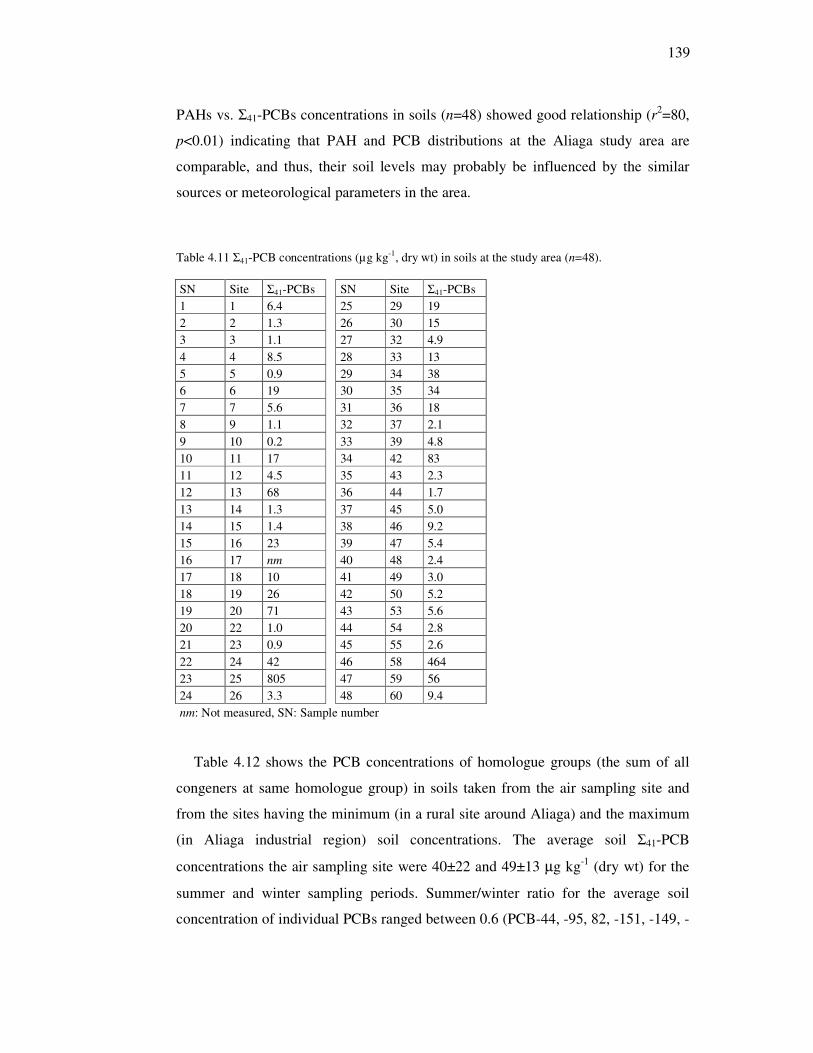
139
PAHs vs. Σ41-PCBs concentrations in soils (n=48) showed good relationship (r2=80,
p<0.01) indicating that PAH and PCB distributions at the Aliaga study area are
comparable, and thus, their soil levels may probably be influenced by the similar
sources or meteorological parameters in the area.
Table 4.11 Σ41-PCB concentrations (µg kg-1, dry wt) in soils at the study area (n=48).
SN Site Σ41-PCBs SN Site Σ41-PCBs
1 1 6.4 25 29 19
2 2 1.3 26 30 15
3 3 1.1 27 32 4.9
4 4 8.5 28 33 13
5 5 0.9 29 34 38
6 6 19 30 35 34
7 7 5.6 31 36 18
8 9 1.1 32 37 2.1
9 10 0.2 33 39 4.8
10 11 17 34 42 83
11 12 4.5 35 43 2.3
12 13 68 36 44 1.7
13 14 1.3 37 45 5.0
14 15 1.4 38 46 9.2
15 16 23 39 47 5.4
16 17 nm 40 48 2.4
17 18 10 41 49 3.0
18 19 26 42 50 5.2
19 20 71 43 53 5.6
20 22 1.0 44 54 2.8
21 23 0.9 45 55 2.6
22 24 42 46 58 464
23 25 805 47 59 56
24 26 3.3 48 60 9.4
nm: Not measured, SN: Sample number
Table 4.12 shows the PCB concentrations of homologue groups (the sum of all
congeners at same homologue group) in soils taken from the air sampling site and
from the sites having the minimum (in a rural site around Aliaga) and the maximum
(in Aliaga industrial region) soil concentrations. The average soil Σ41-PCB
concentrations the air sampling site were 40±22 and 49±13 µg kg-1 (dry wt) for the
summer and winter sampling periods. Summer/winter ratio for the average soil
concentration of individual PCBs ranged between 0.6 (PCB-44, -95, 82, -151, -149, -

140
132) and 2.3 (PCB-191). The overall average soil Σ41-PCB concentration at the air
sampling site (44±17 µg kg-1, dry wt) was relatively low as compared to the highest
soil concentration measured at the industrial site (805 µg kg-1, dry wt). This can be
attributed to its location with respect to the prevailing wind direction.
Table 4.12 Soil concentrations of PCB homologue groups (µg kg-1, dry wt) at the air sampling site and
at the sites having minimum (rural) and maximum (industrial) PCB levels in the study area.
Air Sampling Site (SN:29)
Summer (n=4) Winter (n=3) Homologue Groups Min. Max. GM M Avg±SD Min. Max. GM M Avg±SD
Rural Site (SN:10)
Industrial Site (SN:25)
Tri-CBs 2.0 5.3 3.2 3.2 3.4±1.4 2.5 5.1 3.7 3.9 3.9±1.3 0.09 133
Tetra-CBs 1.7 7.8 4.3 5.0 4.9±2.5 4.9 8.1 6.2 6.0 6.3±1.6 0.07 144
Penta-CBs 2.7 18 9.3 12 11±6.3 13 20 15 14 16±3.7 0.04 215
Hexa-CBs 2.7 20 10 14 13±7.2 14 22 17 15 17±4.3 0.03 234
Hepta-CBs 1.3 9.2 4.9 7.0 6.1±3.4 3.5 6.1 4.4 3.8 4.5±1.4 nd 69
Octa-CBs 0.3 2.0 1.1 1.7 1.4±0.8 0.8 1.5 1.0 0.9 1.1±0.3 nd 9.6
Nona-CBs 0.2 0.7 0.4 0.5 0.5±0.2 0.2 0.5 0.3 0.4 0.4±0.1 nd 1.0
PCB-209 0.1 0.2 0.1 0.1 0.1±0.05 0.06 0.07 0.07 0.1 0.07±0.004 nd 0.2
∑41-PCBs 11 63 34 44 40±22 41 63 48 42 49±13 0.2 805
nd: Not detected, SN: Site number, GM: Geometric mean, M: Median.
PCB homologue profiles in soil samples taken from the industrial site and air
sampling site were similar (r2=0.87, p<0.01) because both sampling points are
relatively close to the steel plants. However, like the PCB profiles in ambient air
samples at remote sites, the PCB profiles in rural soil were dominated by the lower
chlorinated PCBs. A statistically significant correlation was found between the PCB
homologue profiles for the air samples and rural soil (r2=0.89, p<0.01). This
suggested that the lower chlorinated PCBs are transported to relatively longer
distances since they are found mainly in the gas-phase.
The overall average PCB homologue profiles in ambient air, dry deposition and
soil samples are illustrated in Fig. 4.19. The tri-, tetra-, penta-, hexa-CBs, and the
fractions of hepta-through PCB-209 accounted for 8, 13, 30, 33 and 16% of Σ41-PCB
concentration in soil taken from the air sampling site. Despite their large contribution
in air samples, the tri- and tetra-CBs accounted for only a small part of the total PCB

141
mass in soil. The difference in air and soil PCB profiles may be due to their gas-
particle distributions and their different partitioning behaviors (i.e. low molecular
weight compounds have relatively low soil-air partition coefficients).
0
10
20
30
40
50
60
3 4 5 6 7 8 9 10
Homologue Groups
Mas
s C
on
trib
uti
on
(%
)
Soil Dry Deposition Air
Figure 4.19 Overall average PCB homologue profiles in air, dry deposition, and soil
samples. Error bars are 1 SD. ( : Not detected).
4.2.3.2 Soil-Air Gas Exchange Fluxes of PCBs
The fugacity ratios and soil-air gas exchange fluxes were calculated at the air
sampling site using the air (n=28) and soil PCB concentrations (n=7) corresponding
to the same sampling periods. For all individual PCBs, QSA values were calculated
using Eq. (3.18) and KOA values used to calculate KSA (Eq. 3.19) was taken from the
literature (discussed above in Section 4.2.1.3). A statistically significant correlation
was found between log KOA and log QSA values of PCB congeners (r2=0.71, p<0.01,
n=844) indicating that the octanol is a good surrogate for soil organic matter (Fig.

142
4.20). Correlations between the log KOA and log QSA values for non-planar and co-
planar congeners (PCB-28, -31, -33, -70, -74, -105, -118, and -156 at mono-ortho
position) were also determined separately. Both correlations were statistically
significant, however the agreement between the log KOA and log QSA values
determined for co-planar congeners was relatively stronger (r2=0.96, m=0.63,
p<0.01, n=8) than those determined for non-planar ones (r2=0.80, m=0.45, p<0.01,
n=25). This was probably due to the enhanced partitioning of co-planar PCBs into
the soil organic matter compared to non-planar ones.
y = 0.57x + 2.37
r2 = 0.71, p <0.01, n =844
5
6
7
8
9
10
11
12
13
5 6 7 8 9 10 11 12 13
log K OA
log
QS
A
Figure 4.20 log KOA vs. log QSA for all PCB congeners.
A propagation of the errors that are associated with the calculation indicated that
the equilibrium is represented by an fS/fA of 1.0±0.26 (i.e. a range of 0.74-1.26). The
fugacity ratios especially for the lower chlorinated congeners including PCB-17, 18,
44, 49, 52, 87, 95, and 110 were inside this uncertainty range for some samples (i.e.
32, 36, 43, 32, 46, 56, 43, and 32%, respectively). For all PCB congeners, 16% of the
data set (n=847) fell inside this equilibrium range. For the rest, the soil and ambient
air were not in equilibrium.

143
Fig. 4.21 shows the relationship between fugacity in air and soil for all congeners.
Estimated fS/fA ratios showed that generally lighter congeners (tri- to penta-CBs) had
a tendency to volatilize from the soil for some samples while the heavier ones (hexa-
to deca-CBs) had a deposition tendency for all samples. Average fugacity ratios
indicated volatilization for the congeners 17, 18, 52, and 82 in summer and 17, 18,
52, 95 in winter. For the rest, soil is a sink with net gas deposition. Cousins & Jones
(1998) reported fugacity ratios slightly above one for PCB-28, -52, -101, -138, and -
153 and lower than one for PCB-180. Backe et al. (2004) also reported fugacity
ratios between 0.3 and 40 for PCB-28, -101, -138, -153 and -180.
1.E-06
1.E-05
1.E-04
1.E-03
1.E-02
1.E-01
1.E+00
1.E+01
1.E-06 1.E-05 1.E-04 1.E-03 1.E-02 1.E-01 1.E+00 1.E+01
f air (ng m-3
)
fso
il (
ng
m-3
)
PCB-18 PCB-17PCB-31 PCB-28PCB-33 PCB-52PCB-49 PCB-44PCB-74 PCB-70PCB-95 PCB-101PCB-99 PCB-87PCB-110 PCB-82PCB-151 PCB-149PCB-118 PCB-153PCB-132 PCB-105PCB-138 PCB-158PCB-187 PCB-183PCB-128 PCB-177PCB-171 PCB-156PCB-180 PCB-170PCB-199 PCB-208PCB-195 PCB-194PCB-206 PCB-209
Figure 4.21 Relationship between the PCB fugacities (f) in air and soil. The solid
diagonal line represents a 1:1 relationship (equilibrium).
For the samples that soil and ambient air were not in equilibrium, the average
estimated uncertainty in the soil-air net gas exchange fluxes (Fnet) by error
propagation ranged between ±43% (PCB-156, -170, -171, -177, -194, -195, -199, -

144
206, -208, -209) and ±65% (PCB-17, -44, -87) with an overall average of ±52%.
Relatively higher uncertainty values for some PCBs (especially lower chlorinated
ones) were probably due to their proximity to equilibrium.
Table 4.13 shows the instantaneous soil-air net gas exchange fluxes (Fnet) and
MTCs for PCB congeners calculated using Eq. (3.20) and (3.21), respectively.
Negative values indicate a net volatilization from soil to air and positive ones
indicate a net deposition from air to soil. The ranges for the average net gas fluxes of
PCB congeners were between -2.5±1.0 (PCB-82) and 148±176 ng m-2 day-1 (PCB-
31) in summer and between 1.1±0.2 (PCB-171) and 44±51 ng m-2 day-1 (PCB-33) in
winter. PCB congeners of 17, 18, 44, 52, 82, 87, and 95 tended to volatilize in
summer but only PCB-17 and -18 had a tendency to volatilize in winter (Fig. 4.22).
This result is consistent with the calculated soil/air fugacity ratios. Air temperature
had a strong influence on the direction and magnitude of the gas-phase fluxes. For
some PCB congeners, a shift from volatilization to deposition was observed in
winter. Generally, summertime gas exchange fluxes were higher than the wintertime
ones, consistent with the increased air concentrations of gas-phase PCB in summer.
171
180209199
194170156
187128
177
18
17
31
3328
52
49
44
74
95
99
101
87 82
151
118
149
132
153
110
70
105
138
158 183
-150
-100
-50
0
50
100
150
PCB Congeners
Fn
et (
ng
m-2
day
-1)
Summer Winter
Figure 4.22 Net gas exchange fluxes (Fnet) of PCBs between soil-air interface. ( : Not detected).

145
Table 4.13 Calculated MTCs (cm s-1) and instantaneous soil-air net gas exchange fluxes (Fnet, ng m-2
day-1) for PCB congeners.
Summer Winter
MTC F net MTC Fnet PCB Congeners Avg±SD Min. Max. Avg±SD Avg±SD Min. Max. Avg±SD
18 0.78±0.21 -70 -383 -142±188 0.96±0.24 -35 -305 -38±189
17 0.78±0.21 -72 1094 -36±381 0.96±0.24 -12 -186 -41±84
31 0.78±0.21 49 580 148±176 0.96±0.24 22 179 36±64
28 0.78±0.21 -55 345 105±164 0.96±0.24 19 173 30±67
33 0.78±0.21 31 265 112±88 0.96±0.24 29 173 44±51
52 0.76±0.21 -50 -240 -102±61 0.94±0.24 -17 -135 11±106
49 0.76±0.21 -25 -96 18±61 0.94±0.24 10 77 13±44
44 0.76±0.21 -14 41 -8.7±29 0.94±0.24 7.8 84 15±43
74 0.76±0.21 11 47 28±8.8 0.94±0.24 -3.1 37 12±12
70 0.76±0.21 17 58 37±11 0.94±0.24 8.4 79 22±26
95 0.74±0.20 6.0 51 -4.2±27 0.93±0.24 -4.5 64 16±39
101 0.74±0.20 -12 48 20±20 0.93±0.24 9.8 68 25±37
99 0.74±0.20 -3.5 15 5.7±6.5 0.93±0.24 3.3 27 9.9±14
87 0.74±0.20 -5.7 -11 -8.1±2.5 0.93±0.24 -2.6 29 6.5±17
110 0.74±0.20 9.3 30 14±11 0.93±0.24 4.2 51 19±26
82 0.74±0.20 -1.8 -3.2 -2.5±1.0 0.93±0.24 -0.4 6.8 1.3±4.2
151 0.73±0.20 7.4 20 14±3.4 0.91±0.24 1.1 17 4.2±5.1
149 0.73±0.20 21 59 37±9.8 0.91±0.24 2.3 43 14±14
118 0.74±0.20 5.7 47 20±10 0.93±0.24 3.3 34 13±12
153 0.73±0.20 7.5 64 34±15 0.91±0.24 2.9 36 14±11
132 0.73±0.20 2.4 21 8.2±4.9 0.91±0.24 1.6 12 5.2±4.0
105 0.74±0.20 2.5 28 7.8±6.8 0.93±0.24 1.2 12 4.6±3.8
138 0.73±0.20 5.9 58 32±14 0.91±0.24 1.7 33 12±12
158 0.73±0.20 1.8 29 6.1±7.5 0.91±0.24 0.7 5.1 2.0±1.5
187 0.71±0.20 5.6 19 13±3.7 0.89±0.24 0.5 6.3 2.6±1.5
183 0.71±0.20 3.0 10 7.1±1.9 0.89±0.24 0.7 3.0 1.6±0.7
128 0.73±0.20 2.6 6.3 3.9±1.1 0.91±0.24 1.3 3.0 2.0±0.9
177 0.71±0.20 3.6 10 6.5±1.8 0.89±0.24 1.0 3.0 1.9±0.6
171 0.71±0.20 1.9 4.7 3.2±0.8 0.89±0.24 0.8 1.3 1.1±0.2
156 0.73±0.20 2.1 9.3 4.4±1.9 0.91±0.24 0.8 1.6 1.2±0.6
180 0.71±0.20 9.0 26 19±5.4 0.89±0.24 1.3 8.1 2.7±1.7
191 0.71±0.20 nc nc nc 0.89±0.24 nc nc nc
169 0.73±0.20 nc nc nc 0.91±0.24 nc nc nc
170 0.71±0.20 6.3 15 10±2.8 0.89±0.24 1.0 4.1 2.1±1.4
199 0.70±0.19 3.1 11 5.8±2.0 0.88±0.24 0.9 1.3 1.1±0.3
208 0.69±0.19 nc nc nc 0.87±0.23 nc nc nc
195 0.70±0.19 nc nc nc 0.88±0.24 nc nc nc
194 0.70±0.19 2.9 5.8 4.1±1.2 0.88±0.24 nc nc nc
205 0.70±0.19 nc nc nc 0.88±0.24 nc nc nc
206 0.69±0.19 nc nc nc 0.87±0.23 nc nc nc
209 0.68±0.19 1.5 6.6 4.0±3.6 0.86±0.23 nc nc nc
nc: Not calculated.
Negative values indicate net gas volatilization from the soil.

146
Table 4.14 Annual fluxes (ng m-2 year-1) and FSA/FAS ratios of PCB congeners.
PCB Congeners
Wet Depositiona
Dry Deposition
Gas Absorption
Gas Volatilization FSA/FAS
18 2,483 15,495 62,758 99,879 1.2
17 991 8,351 49,256 63,150 1.1
31 1,974 9,701 63,801 32,629 0.4
28 1,731 10,222 60,367 38,614 0.5
33 706 16,195 46,766 19,307 0.3
52 572 11,713 37,929 55,835 1.1
49 710 12,366 26,734 21,092 0.5
44 110 9,976 17,663 15,890 0.6
74 nd 9,365 11,171 3,916 0.2
70 198 7,682 18,026 7,384 0.3
95 245 5,554 14,839 12,512 0.6
101 303 6,224 19,972 11,901 0.5
99 91 3,818 6,863 4,174 0.4
87 593 11,086 6,373 5,329 0.3
110 255 7,107 12,921 7,046 0.4
82 5.9 6,018 1,595 1,374 0.2
151 54 3,150 4,303 1,169 0.2
149 295 6,547 12,191 3,194 0.2
118 120 7,099 8,090 1,945 0.1
153 84 8,151 11,709 2,748 0.1
132 2.3 5,247 3,213 719 0.08
105 nd 5,356 2,912 663 0.08
138 20 14,325 11,452 3,448 0.1
158 nd nd 1,714 265 0.2
187 28 4,497 3,359 523 0.07
183 2.3 nd 1,844 261 0.1
128 nd nd 3,011 1,780 0.6
177 nd 3,842 1,829 168 0.03
171 nd nd 1,092 115 0.1
156 nd nd 1,534 133 0.09
180 5.9 8,776 4,281 389 0.03
170 nd 9,821 3,210 173 0.01
199 nd nd 1,921 59 0.03
194 nd nd 1,504 20 0.01
209 nd nd 1,472 1.6 0.001
ΣPCBs 11,577 227,682 537,678 417,804
nd: Not detected. a Odabasi, 2007b.
Table 4.14 shows the annual average fluxes of PCB congeners and the ratios of
total fluxes representing soil to air (FSA, i.e. gas volatilization) and air to soil (FAS,
i.e. gas absorption, dry and wet deposition) processes. Gas absorption and
volatilization fluxes were calculated using Eq. (3.20). Wet deposition fluxes
147
measured recently at a suburban site of Buca in Izmir during autumn 2005-spring
2006 (Odabasi, 2007b) were also used to estimate relative importance of different
atmospheric processes. All processes were comparable for Σ35-PCBs but their input
was dominated by gas absorption with a contribution of 69%. Dry deposition
accounted for 29% of the atmospheric Σ35-PCB inputs and was followed by wet
deposition with a contribution of only 1%. The calculated ratios of PCB-17, -18, and
-52 were slightly above 1.0 suggesting that for these congeners, soil and air may be
approaching a steady state condition. For the remaining congeners, there was a net
accumulation into the soil.
4.3 Organochlorine Pesticides (OCPs)
4.3.1 OCPs in Ambient Air
4.3.1.1 Ambient Air Concentrations of OCPs
Atmospheric pesticide concentrations measured at this study are summarized in
Table 4.15. Dieldrin, endrin, endrin aldehyde, endrin ketone, and methoxychlor in
the air samples (n=28) were under their detection limits for both sampling periods.
For the rest, average total (gas+particle) concentrations ranged between 0.2±0.05 (c-
nonachlor) and 2152±2974 pg m-3 (endosulfan-I) in summer, and between not
detected (nd) (δ-HCH, c-nonachlor) and 121±160 pg m-3 (chlorpyrifos) in winter
(average±SD).
Endosulfan-I had the highest average total concentration in summer, and was
followed by endosulfan-II, and chlorpyrifos. In winter, major OCPs in air were
chlorpyrifos, α-HCH, and endosulfan-I, respectively (Table 4.15). Measured high
endosulfan and chlorpyrifos levels may probably due to their current uses in Turkey.

148
148
Table 4.15 Atmospheric concentrations (pg m-3) of OCP compounds at the air sampling site (1/2).
Summer
Particle-Phase Gas-Phase Total (Gas+Particle)
OCPs Min. Max. Geometric Mean Median Avg±SD Min. Max.
Geometric Mean Median Avg±SD Min. Max.
Geometric Mean Median Avg±SD
α-HCH 1.8 8.3 3.5 3.5 4.0±2.0 28 190 93 94 102±43 34 193 97 99 106±43
β-HCH 2.0 10 4.5 6.2 6.2±6.0 3.5 20 10 12 12±6.0 3.5 31 11 12 14±9.1
γ-HCH 1.4 8.0 3.7 3.6 4.2±2.1 21 76 42 41 44±16 26 82 46 44 49±16
δ-HCH 0.6 4.8 1.4 1.3 1.8±1.3 1.5 4.0 2.5 2.6 2.6±0.8 1.0 8.8 2.4 2.4 2.8±1.9
CHLPYR 2.8 17 6.3 6.8 7.1±3.7 16 689 80 75 135±178 21 706 89 80 143±181
HEP EPOX 0.2 3.9 1.0 1.0 1.3±1.1 2.2 10 4.6 4.6 5.0±2.3 2.2 13 5.4 5.9 6.0±3.0
α-CHL 0.1 0.4 0.2 0.2 0.2±0.1 1.3 5.7 2.7 3.0 2.9±1.3 1.3 6.2 2.8 3.0 3.0±1.4
γ-CHL 0.03 0.3 0.1 0.2 0.1±0.07 0.8 2.6 1.6 1.6 1.6±0.5 0.8 2.8 1.7 1.7 1.7±0.6
c-NONA nd nd nd nd nd 0.1 0.2 0.2 0.2 0.2±0.05 0.1 0.2 0.2 0.2 0.2±0.05
t-NONA 0.03 0.1 0.05 0.04 0.05±0.04 0.7 2.1 1.2 1.2 1.3±0.4 0.7 2.1 1.2 1.2 1.3±0.4
ESLF-I 3.5 22 8.5 8.1 9.9±5.8 481 11704 1325 950 2142±2970 487 11726 1336 961 2152±2974
ESLF-II 5.5 109 19 13 29±31 66 1362 186 154 271±338 76 1422 213 201 300±351
ESLF SUL 1.6 12 3.4 3.1 4.2±3.1 4.8 60.9 10.0 9.3 13±14 6.4 73 14 14 17±16
p,p'-DDT 3.8 32 9.5 8.9 12±8.5 21 81 43 44 46±17 30 87 56 56 58±16
p,p'-DDD 1.0 5.1 2.6 2.6 2.8±1.1 6.9 26 16 17 17±5.3 10 27 19 20 19±4.7
nd: Not detected.
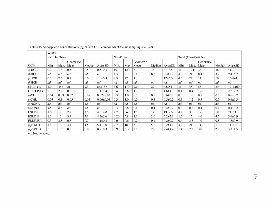
149
149
Table 4.15 Atmospheric concentrations (pg m-3) of OCP compounds at the air sampling site (2/2).
Winter
Particle-Phase Gas-Phase Total (Gas+Particle)
OCPs Min. Max. Geometric Mean Median Avg±SD Min. Max.
Geometric Mean Median Avg±SD Min. Max.
Geometric Mean Median Avg±SD
α-HCH 0.2 1.3 0.5 0.5 0.5±0.3 10 123 33 36 41±32 11 124 33 36 41±32
β-HCH nd nd nd nd nd 4.3 21 8.4 8.2 9.4±5.2 4.3 21 8.4 8.2 9.4±5.2
γ-HCH 0.3 2.6 0.7 0.6 1.0±0.8 4.3 27 11 10 12±6.3 4.3 27 11 10 13±6.4
δ-HCH nd nd nd nd nd nd nd nd nd nd nd nd nd nd nd
CHLPYR 1.9 457 21 9.3 86±137 3.6 170 22 22 42±54 11 481 53 39 121±160
HEP EPOX 0.3 2.9 0.6 0.3 1.1±1.4 0.4 5.6 1.3 1.2 1.6±1.3 0.4 8.4 1.6 1.3 2.2±2.2
α-CHL 0.04 0.09 0.07 0.08 0.07±0.03 0.3 1.0 0.5 0.5 0.6±0.2 0.3 1.0 0.5 0.5 0.6±0.2
γ-CHL 0.03 0.1 0.05 0.04 0.06±0.04 0.3 1.0 0.5 0.5 0.5±0.2 0.3 1.2 0.5 0.5 0.6±0.3
c-NONA nd nd nd nd nd nd nd nd nd nd nd nd nd nd nd
t-NONA nd nd nd nd nd 0.3 0.8 0.4 0.4 0.4±0.2 0.3 0.8 0.4 0.4 0.4±0.2
ESLF-I 1.0 12 2.7 2.5 4.0±4.0 4.7 36 17 17 19±9.3 4.7 38 19 18 21±11
ESLF-II 1.3 13 3.4 3.1 4.3±3.6 0.20 5.8 1.1 2.0 2.2±2.1 1.6 15 4.6 4.5 5.6±3.9
ESLF SUL 0.3 2.8 0.8 0.7 1.1±0.8 0.04 0.6 0.2 0.1 0.2±0.2 0.4 3.3 1.0 0.8 1.3±0.9
p,p'-DDT 1.4 13 4.4 4.5 5.1±3.0 2.7 18 5.3 5.2 6.2±4.1 4.9 21 11 11 11±4.6
p,p'-DDD 0.3 1.6 0.8 0.8 0.9±0.3 0.9 6.3 2.1 2.0 2.4±1.4 1.4 7.2 3.0 2.9 3.3±1.5
nd: Not detected.

150
Total (gas+particle) atmospheric concentrations of individual OCPs measured at
this study were within the range of those previously reported values in Table 2.6.
Atmospheric OCP levels that were found at a remote site in Germany (Wenzel et al.,
2006), at the Arctic atmosphere (Hung et al., 2005), and at a rural/forested site in
USA (Gioia et al., 2005) were lower than the obtained results. At a coastal/urban site
of Izmir, Odabasi et al. (2008) reported generally higher atmospheric OCP
concentrations in the summer and winter sampling periods, excepting p,p'-DDT, p,p'-
DDD, and α, β, δ isomers of HCH which were measured higher at this study.
Sofuoglu et al. (2004) also reported higher values of OCPs in spring at a suburban
site of Izmir, except for endosulfan-I, endosulfan-II, p,p'-DDT and p,p'-DDD which
were found higher in the summer sampling period of this study. Similarly,
chlorpyrifos and endosulfan had the highest atmospheric concentrations among the
OCPs measured in Izmir air (Odabasi et al., 2008; Sofuoglu et al., 2004).
γ-HCH released into the atmosphere both as lindane (pure γ-HCH) and as a
component of technical HCH comprised of 60-70% α-HCH, 5-12% β-HCH, 10-15%
γ-HCH, 6-10% δ-HCH, and other isomers (ATSDR, 2005). The uses of technical
HCH and lindane have been banned for decades in Turkey (Acara et al., 2006).
However, lindane is currently used in Europe (Lee et al., 2000; Wania et al., 1998). It
was reported by Murayama et al. (2003) and Lee et al. (2000) that α- to γ-HCH ratio
was close to 1 in areas where γ-HCH was used, and between 3-7 in areas where α-
HCH was used or in remote areas. In this study, the average α- to γ-HCH ratio was
2.1±0.4 in summer and 3.1±0.9 in winter, indicating the effect of remote sources on
the ambient HCH levels at the study site. Lower α- to γ-HCH ratio in summer may
be related to the elevated atmospheric concentrations of γ-HCH during this period
(Table 4.15). At the other studies performed in Izmir, relatively low average α- to γ-
HCH ratios were found to be 1.1±0.3 for the coastal/urban site (Odabasi et al, 2008)
and 1.2±0.5 for the suburban site (Sofuoglu et al., 2004). This may be due to higher
atmospheric γ-HCH levels measured at coastal/urban and suburban sites in Izmir
than those measured at the air sampling site in Aliaga (Table 2.6). Manz et al. (2001)
reported that HCHs can be emitted by hazardous waste dumps, cable scrapping and
incineration in smelting plants because of the previous usage of HCHs as an additive

151
in plasticizer production (e.g. in PVC sheathing of electric cables). At the iron-steel
plants located in the Aliaga industrial region, all kinds of scrap iron materials are
stored, classified, cut into parts, and melted. Therefore, relatively high α- to γ-HCH
ratios in the air may also be due to high α-HCH levels at the air sampling site
released from nearby iron-steel plants smelting of scrap materials contained PVC
sheathed cables.
Technical endosulfan contains 70% of endosulfan-I and 30% of endosulfan-II.
Endosulfan sulfate is their main degradation product (Hafner & Hites, 2003).
Sofuoglu et al. (2004) reported the usage of endosulfan/chlorpyrifos ratio in Izmir
area was 7.5. The average ratio of endosulfan-I and -II to chlorpyrifos in air was
23±16 in summer and 1.0±1.3 in winter. When endosulfan sulfate was included,
seasonal ratios were almost not changed because of its little contribution (~3%) to
Σendosulfan (endosulfan-I, -II, and endosulfan sulfate) mass in air for both seasons.
Observed high Σendosulfans/chlorpyrifos ratio in summer can be attributed to the
high regional and local applications of endosulfan during the summer months.
Relatively low atmospheric Σendosulfans/chlorpyrifos ratio in winter may be due to
different properties of these compounds (i.e. vapor pressure, octanol-air partition
coefficient, and reactivity in the air) and their different seasonal uses for the
agricultural purposes.
γ(trans)- to α(cis)-CHL ratio of ~1.2 in the technical chlordane and <1 in the
Arctic atmosphere were reported by Hung et al. (2005). In Turkey, the use of
chlordane was banned in 1979. The average ratio of atmospheric γ-/α-CHL at the air
sampling site was found to be 0.7±0.2 in summer and 1.0±0.5 in winter suggesting
that there was no fresh usage of chlordane-based pesticides in this area.
The correlations between the atmospheric total concentrations of related
pesticides are illustrated in Fig. 4.23. Statistically significant correlation (p<0.01)
was found between α- and γ-HCH isomers; γ-chlordane and other chlordane related
compounds (heptachlorepoxide, α-chlordane, c-nonachlor, t-nonachlor); endosulfan-I

152
and other endosulfan related compounds (endosulfan-II, endosulfan sulfate); p,p'-
DDT and p,p'-DDD in air samples (n=28). This indicates that the related OCPs in air
are possibly affected by the same source and/or local processes in the ambient
environment under the given meteorological conditions. However, there was a
relatively weak correlation (p<0.05-0.10) between α-HCH and β, δ isomers. This
might be because of their remote sources.
y = 0.41x + 0.71
r2 = 0.85, p <0.01
y = 0.06x + 6.45
r2 = 0.23, p <0.05
y = 0.02x + 0.34
r2 = 0.26, p <0.10
0
10
20
30
40
50
60
70
80
90
0 50 100 150 200 250
a-HCH
CA (
pg m
-3)
b-HCH
g-HCH
d-HCH
y = 0.12x + 20.95
r2 = 0.98, p <0.01
y = 0.01x + 2.99
r2 = 0.92, p <0.01
0
200
400
600
800
1000
1200
1400
1600
0 2000 4000 6000 8000 10000 12000 14000
ESLF-I
C A (pg m-3)
CA (
pg m
-3)
ESLF-II
ESLF SUL
y = 3.01x + 0.06
r2 = 0.71, p <0.01
y = 1.54x - 0.21
r2 = 0.85, p <0.01
y = 0.67x + 0.09
r2 = 0.82, p <0.01
y = 0.08x + 0.03
r2 = 0.76, p <0.01
0
2
4
6
8
10
12
0 1 2 3 4g-CHL
HEP EPOX
a-CHL
t-NONA
c-NONA
y = 0.32x + 0.43
r2 = 0.87, p <0.01
0
5
10
15
20
25
30
0 20 40 60 80 100
p-p'-DDT
C A (pg m-3)
p-p'-DDD
Figure 4.23 Correlations between the atmospheric total concentrations (CA) of related pesticides.
Summertime average total concentrations for all of the studied OCPs in air were
higher than the wintertime ones (Table 4.15). The summer/winter ratios were
between 1.1 (chlorpyrifos) and 93 (endosulfan-I). Measured high atmospheric OCP
levels in summer may be related to the enhanced local/regional applications of in-use
pesticides and enhanced volatilization rates of the compounds during hot summer

153
months. Similar increases in atmospheric pesticide concentrations during summer
were also reported by Cortes et al. (1999), Gioia et al. (2005), Halsall et al. (1998),
Harrad & Mao (2004), Lee et al. (2000), Odabasi et al. (2008), and Sun et al. (2006).
Summer
0
20
40
60
80
100
120P
hase
Dis
trib
utio
n (%
)
Gas Particle
Winter
0
20
40
60
80
100
120
α-H
CH
β-H
CH
γ-H
CH
δ-H
CH
CH
LP
YR
HE
P E
PO
X
α-C
HL
γ-C
HL
c-N
ON
A
t-N
ON
A
ES
LF
-I
ES
LF
-II
ES
LF
SU
L
p,p'
-DD
T
p,p'
-DD
D
OCPs
Pha
se D
istr
ibut
ion
(%)
Figure 4.24 Average phase distributions of individual pesticides for the summer and
winter periods. Error bars are 1 SD. ( : Not detected).
Average OCP concentrations measured in particle-phase ranged between nd (c-
nonachlor) and 29±31 pg m-3 (endosulfan-II) in summer, and between nd (β-HCH, δ-

154
HCH, c-nonachlor, t-nonachlor) and 86±137 pg m-3 (chlorpyrifos) in winter. For the
gas-phase, they ranged between 0.2±0.05 (c-nonachlor) and 2142±2970 pg m-3
(endosulfan-I) in summer, and between nd (δ-HCH, c-nonachlor) and 42±54 pg m-3
(chlorpyrifos) in winter (Table 4.15). Generally, gas-phase percentages for individual
pesticides were higher in summer than in winter, probably due to increased
partitioning of compounds to gas-phase with temperature (Fig. 4.24).
4.3.1.2 Influence of Meteorological Parameters on OCP Levels in Air
The relationship between the air temperature and gas-phase partial pressure of
individual pesticides in the air was evaluated using Eq. (3.1). The temperature
dependency of gas-phase concentrations was statistically significant (p<0.01) for all
of the studied pesticides except β-HCH, and changes in temperature accounted for 7
(β-HCH) to 94% (endosulfan-II) of the variability in gas-phase concentrations. The
regression slopes between -1458 (β-HCH) and -32944 (endosulfan-II) were found to
be rather steep and were consistent with those derived from other recent studies
(Halsall et al., 1998; Harrad & Mao, 2004; Lee et al., 2000; Yeo et al., 2003).
Among the studied pesticides, endosulfan-I, -II, and endosulfan sulfate had the
highest slopes and r2 values, supporting their seasonal variations in gas-phase
concentrations. The slopes and r2 values for α- and γ-HCH were found to be -5154,
0.39 and -6707, 0.61, respectively. This result is supported by Wania et al. (1998)
indicating that gas-phase γ-HCH concentrations in air display stronger temperature
dependencies than those of α-HCH and r2 value of γ-HCH often exceeds 0.5.
Eq. (3.2) was performed to assess the influence of wind speed and wind direction
on gas-phase OCP concentrations in air. Temperature, wind speed, and wind
direction, altogether, accounted for 20 to 94% of the variability in the atmospheric
concentrations of gas-phase OCPs (Table 4.16). Negative m1 and m2 values indicated
that the gas-phase concentrations increased with temperature and decreased with
wind speed, respectively. Steep slopes (m1) suggested that the gas-phase
concentrations were influenced by regional or short-range transport and by

155
volatilization from contaminated surfaces. Positive m3 values are associated with
northerly winds while negative values point southerly directions for relatively higher
gas-phase concentrations. The low significance (p>0.10) of the MLR analysis for m1,
m2, m3 parameters indicated the lack of correlation between the meteorological
parameters and the gas-phase air concentrations of β-HCH. This indicates that its
gas-phase concentrations might be transported from remote areas.
Table 4.16 Summary of regression parameters for Eq. (3.2).
OCPs m1 m2 m3 r2 n
α-HCH -3674a -0.22a 0.60a 0.71 28
β-HCH -1533 -0.07 0.73 0.20 18
γ-HCH -6083a -0.14a 0.69a 0.81 28
CHLPYR -6416a 0.01 0.18 0.23 28
HEP EPOX -7663a 0.09 0.44 0.59 28
α-CHL -8558a -0.05 0.21 0.86 26
γ-CHL -5775a -0.08a 0.47a 0.78 28
c-NONA -22511b 0.22 -0.06 0.76 11
t-NONA -5801a -0.06a 0.06 0.85 28
ESLF-I -24116a 0.09 0.73b 0.89 28
ESLF-II -32458a -0.10 0.20 0.94 22
ESLF SUL -22751a 0.04 0.49 0.92 28
p,p'-DDT -11016a -0.05 0.22 0.88 28
p,p'-DDD -10674a -0.05 0.34 0.87 28 a p<0.05.
b p<0.10.
4.3.1.3 Gas-Particle Partitioning of OCPs
Temperature dependent KOA values for individual pesticides were calculated using
the regression parameters reported by Shoeib & Harner (2002). The parameters that
were not available for chlorpyrifos, heptachlorepoxide, endosulfan-II, and endosufan
sulfate were taken from Odabasi (2007a). PL values for OCPs as a function of
temperature were also calculated using the regression parameters given by Hlnckley,
Bidleman, Foreman, & Tuschall (1990). The parameters that were not available for
heptachlorepoxide and chlorpyrifos were taken from Odabasi (2007a).

156
The experimental KP values for OCPs were determined using Eq. (3.6) and they
were plotted against log PL and log KOA. For individual samples, r2 values were
between 0.03-0.72 for PL and 0.07-0.62 for KOA. Regression parameters, m and b,
were -0.10 to -0.81 and -3.04 to -5.39 for PL and 0.15 to 0.84 and -4.10 to -10.73 for
KOA, respectively. The variation in slopes indicated that atmospheric particles for
different samples have different sorbing properties (Sofuoglu et al., 2004). Observed
slopes and r2 values in regression of log KP vs. log KOA and log KP vs. log KOA for
OCPs were almost the same suggesting that both PL and KOA values can be used to
describe the partitioning of OCPs between gas- and particle-phases. Figure 4.25
shows the plots of measured log KP vs. log PL and log KP vs. log KOA values of
pesticides for all sample events. Statistically significant correlation was found for PL
(r2=0.28, p<0.01, n=229) and for KOA (r2=0.28, p<0.01, n=230). However, the slopes
of regression lines, -0.41 and 0.41, were different from the expected value of -1 and
1, respectively. Similarly, Sofuoglu et al. (2004) conducted a study on gas-particle
partitioning of OCPs at suburban Izmir and found the regression slope of 0.46 in log
KP vs. log KOA correlation for all samples.
y = -0.41x - 3.88
r2 = 0.28
-6
-5
-4
-3
-2
-1
0
1
-6 -5 -4 -3 -2 -1 0 1
log P L
log
KP (
Mea
sure
d)
y = 0.41x - 6.66
r2 = 0.28
6 7 8 9 10 11 12 13
log K OA
Figure 4.25 Plots of log KP measured at the air sampling site vs. log PL and log KP vs. log KOA for
all samples. The solid diagonal line represents a 1:1 relationship (equilibrium).

157
Fig. 4.26 compares the experimentally determined (Eq. 3.6) and modeled (Eq.
3.13) log KP values of OCPs for all samples. The relationship between the modeled
and measured partition coefficients was good (r2=0.27, p<0.01, n=230). However,
the results indicated that KOA based model under-predicts the experimental KP values
for α-HCH, γ-HCH, chlorpyrifos, heptachlorepoxide, endosulfan-II, and endosulfan
sulfate while over-predicts for t-nonachlor and p,p'-DDD. Generally, predicted
partition coefficients for endosulfan-I, p,p'-DDT, α-chlordane, and γ-chlordane were
good. The range of average measured/modeled KP values for individual pesticides
was from 0.3±0.2 (p,p'-DDD) to 30±27 (γ-HCH), and for all OCP compounds,
overall average ratio was 10±22.
y = 0.42x - 1.53
r2 = 0.27, p <0.01, n =230
-6
-5
-4
-3
-2
-1
0
-6 -5 -4 -3 -2 -1 0
log K P (Modeled)
log
KP (
Exp
erim
enta
l)
Figure 4.26 Correlation between the measured and predicted
log KP values of OCPs. The solid diagonal line represents a
1:1 relationship (equilibrium).
The fraction (φ) of OCPs in particle-phase was calculated experimentally using
Eq. (3.4). Fig. 4.27 compares the average measured particle fraction (100×φ) of
pesticides with the ones predicted by Junge-Pankow adsorption (Eq. 3.8) and KOA

158
absorption models (Eq. 3.7). Experimental φ values were correlated with the ones
predicted by Junge-Pankow adsorption and KOA absorption model for all data set,
and statistically significant relationships were found (r2=0.35, p<0.01, n=253, and
r2=0.34, p<0.01, n=230, respectively).
0
10
20
30
40
50
60
-4 -3.5 -3 -2.5 -2 -1.5 -1 -0.5
log P L
Par
ticl
e F
ract
ion
(%)
Experimental
Junge-Pankow
7.5 8 8.5 9 9.5 10 10.5 11
log K OA
Experimental
Koa-Based
Figure 4.27 Comparison of measured particle fraction of OCPs with Junge-Pankow adsorption
and KOA absorption model.
Generally, all of the studied pesticides were mainly in gas-phase with a range of
average predicted particulate fractions (100×φ) between 0.33 (α-HCH) and 55%
(p,p'-DDD). Although the relationship between the measured and predicted φ values
was good, particulate fractions were predicted lower than their experimental results
for α-HCH, γ-HCH, chlorpyrifos, heptachlorepoxide, γ-chlordane, endosulfan-II, and
endosulfan sulfate. Good predictions were generally observed for α-chlordane, t-
nonachlor, p,p'-DDT, and p,p'-DDD from Junge-Pankow adsorption model, and for
α-chlordane, endosulfan-I, and p,p'-DDT from KOA absorption model. The average
ratio of measured/predicted φ values for individual OCPs ranged from 0.5±0.4
(endosulfan-I) to 44±61 (α-HCH) for Junge-Pankow model, and from 0.4±0.2 (t-
nonachlor, p,p'-DDD) to 26±22 (γ-HCH) for KOA model. For all of the studied OCPs,
it was 10±25 and 7±13, respectively. Sofuoglu et al. (2004) used KOA model to
estimate the particulate percentages of OCPs at suburban Izmir and they reported
good predictions for β-HCH, endosulfan-I, and p,p'-DDT, and under-predicted
particulate percentages for α-HCH, γ-HCH, chlorpyrifos, and dieldrin.

159
4.3.2 Particle-Phase Dry Deposition Fluxes and Velocities of OCPs
Particle-phase OCP dry deposition fluxes (Fd, ng m-2 day-1) were measured
experimentally using dry deposition plates, and calculated using Eq. (3.16). The
range for the average Fd values of individual pesticides was between 1.1±1.2 (t-
nonachlor) and 503±455 ng m-2 day-1 (endosulfan-I) in summer and between 0.3±0.3
(t-nonachlor) and 110±157 ng m-2 day-1 (chlorpyrifos) in winter (Table 4.17).
Generally, particle fluxes were higher in summer than in winter. Summer/winter
ratios for the average Fd values of individual pesticides were between 0.4
(chlorpyrifos) and 32 (endosulfan-I). This result is consistent with particle-phase
concentrations of OCPs (except chlorpyrifos) that were measured higher in summer
than in winter (Table 4.15).
Table 4.17 Particle-phase dry deposition fluxes (Fd) and velocities (Vd) of individual OCPs.
Fd (ng m-2 day-1) Vd (cm s-1)
Summer Winter Overall
OCPs Min. Max. GM M Avg±SD Min. Max. GM M Avg±SD GM M Avg±SD
α-HCH 2.5 14 5.5 5.5 6.3±3.5 2.0 20 6.0 5.3 7.7±6.0 3.4 3.6 5.8±5.8
γ-HCH 3.8 29 8.2 7.6 9.7±6.9 4.1 16 6.2 5.3 6.9±3.9 3.8 5.1 4.8±3.1
CHLPYR 7.4 207 30 27 47±57 13 573 53 36 110±157 3.9 3.6 5.4±4.5
HEP EPOX 3.7 46 9.7 10 14±14 1.2 23 5.3 6.0 9.5±9.3 4.4 4.3 4.6±1.4
α-CHL 0.9 4.5 2.0 2.0 2.3±1.5 0.3 1.0 0.6 0.6 0.6±0.2 9.7 11 10±3.3
γ-CHL 0.1 11 0.8 0.7 1.7±3.3 0.1 1.5 0.6 0.5 0.7±0.5 6.1 6.7 8.1±5.3
t-NONA 0.4 2.8 0.8 0.6 1.1±1.2 0.1 0.5 0.3 0.3 0.3±0.3 11 11 11±5.1
ESLF-I 184 1715 375 265 503±455 4.5 38 12 9.1 16±13 6.7 6.7 8.2±5.3
ESLF-II 36 435 99 76 138±133 1.1 29 4.1 3.1 6.5±7.6 3.0 3.8 4.4±3.9
ESLF SUL 4.7 37 11 9.1 13±10 0.3 4.6 1.2 1.4 1.6±1.1 2.4 2.2 2.8±1.6
p,p'-DDT 9.7 210 19 16 31±52 4.1 164 14 11 23±41 2.7 2.5 3.3±2.5
p,p'-DDD 2.1 51 5.8 5.0 8.4±12 3.0 6.8 4.3 4.3 4.4±1.2 3.8 4.1 4.6±3.0
ΣOCPs 3.5 3.6 4.9±4.1
GM: Geometric mean, M: Median.
No previous measurement of particle-phase OCP dry deposition fluxes obtained
with experimental techniques was available for comparison. However, there have
been several studies on OCP dry deposition fluxes that were calculated using indirect
method. At a coastal/urban site in Izmir, Odabasi et al. (2008) estimated particle
fluxes of pesticides taking dry deposition velocities of OCPs that were determined

160
recently for urban and suburban sites in Izmir. They reported Fd values ranging
between 0.6 (c-nonachlor) and 388 (chlorpyrifos) ng m-2 day-1. Gioia et al. (2005)
also assumed a deposition velocity of 0.5 cm s-1 to calculate Fd values of OCPs at the
different sites in New Jersey. The calculated fluxes for Σchlordanes, ΣDDTs,
endosulfan-I, -II, and endosulfan sulfate were 2.8, 1.5, 0.9, 1.8, and 0.7 ng m-2 day-1
for urban/industrial site; 1.8, 1.2, 0.2, 0.9, and 0.4 ng m-2 day-1 for suburban site; and
0.5, 0.3, 0.4, 0.9, and 0.6 ng m-2 day-1 for rural/forested site, respectively.
Currently used pesticides in Turkey, endosulfan and chlorpyrifos, had a large
fraction in particle fluxes of OCPs at the air sampling site, like their large
contributions to total OCP mass in air. Among the studied pesticides, endosulfan-I
had the highest average deposition flux in summer and was followed by endosulfan-
II and chlorpyrifos. In winter, they were chlorpyrifos, p,p'-DDT, and endosulfan-I,
respectively. Similarly, Odabasi et al. (2008) reported the highest particle fluxes for
in-use pesticides of chlorpyrifos and endosulfan in coastal/urban Izmir.
Particle-phase dry deposition velocities (Vd, cm s-1) for individual pesticides were
calculated using measured dry deposition fluxes and atmospheric particle-phase
concentrations (Eq. 3.17). The range for the Vd values was between 2.3±1.4 (α-HCH)
and 11±5.1 (t-nonachlor) cm s-1 in summer, and between 1.6±1.0 (endosulfan-II) and
13±4.7 (α-HCH) cm s-1 in winter. The overall average deposition velocities were
4.6±3.6 and 5.3±4.6 cm s-1 for the summer and winter sampling periods,
respectively. The seasonal difference in Vd values may be due to different size
distributions and meteorological variables observed for both seasons.
For both sampling periods, the correlation between the dry deposition fluxes and
atmospheric particulate concentrations was statistically significant (r2=0.73, p<0.01,
n=112 for summer; r2=0.88, p<0.01, n=98 for winter; and overall r2=0.63, p<0.01,
n=210). The overall average Vd values for individual pesticides varied from 2.8±1.6
(endosulfan sulfate) to 11±5.1 cm s-1 (t-nonachlor). This value was 4.9±4.1 cm s-1 for
all of the studied pesticides (Table 4.17).

161
Particulate deposition velocities for other SOCs have been studied extensively.
Reported overall average Vd values in Table 2.9 ranged between 0.4-6.7 cm s-1 for
PAHs (Demircioglu, 2008; Esen et al., 2008; Tasdemir & Esen, 2007b; Vardar et al.,
2002; Odabasi et al., 1999a; Franz et al., 1998) and between 0.7-7.2 cm s-1 for PCBs
(Esen et al., 2008; Cindoruk & Tasdemir 2007b; Tasdemir & Holsen, 2005;
Tasdemir et al., 2004b; Franz et al., 1998). Thus, the overall average Vd value in this
study (4.9±4.1 cm s-1) is consistent with those reported values for other SOCs.
4.3.3 OCPs in Soil
4.3.3.1 Soil Concentrations of OCPs
Among the collected sample matrices (i.e. soil, ambient air, dry deposition), p,p'-
DDE was only analyzed for the soil samples taken from 48 different points in the
study area. γ-HCH, α- CHL, γ-CHL, t-nonachlor, endosulfan-I, endosulfan-II,
endosulfan sulfate, p,p'-DDT, p,p'-DDD, and p,p'-DDE were the most abundant
compounds found in 100% of the soil samples (n=48), and they were followed by α-
HCH (%98), c-nonachlor (%96), chlorpyrifos (%92), heptachlorepoxide (%77), β-
HCH (%27), δ-HCH and dieldrin (%15), and endrin (%2). Endrin aldehyde, endrin
ketone, and methoxychlor were under their detection limits (n=48).
Table 4.18 shows the related pesticide concentrations in soils (n=48) at the study
area. These values are relatively high in comparison with those previously reported
in Table 4.12. Soil concentrations of related pesticides showed a large variation
between the sampling points, probably due to differences in pesticide application
histories and dissipation rates. They ranged between 0.3-4157 µg kg-1 (dry wt) for
ΣDDX, 0.09-26 µg kg-1 (dry wt) for Σendosulfans, 0.008-35 µg kg-1 (dry wt) for
Σchlordanes, nd-6.8 µg kg-1 (dry wt) for chlorpyrifos and 0.007-2.3 µg kg-1 (dry wt)
for ΣHCHs (Table 4.18). The highest levels in soils were generally found for ΣDDX,
in agreement with the recent studies (Bidleman & Leone, 2004; Meijer et al., 2003a;
Harner et al., 1999). The formulation of technical DDT mainly contains 65-80% of

162
p,p'-DDT. p,p'-DDD and p,p'-DDE are impurities in technical DDT as well as its
degradation products. Because of their extremely low water solubility and their high
organic carbon partition coefficients (KOC), DDT and its metabolites are essentially
immobile in soil, becoming strongly absorbed onto the surface layer of soils (UNEP,
2006). In Turkey, the use of DDT was restricted in 1978, and then, it was prohibited
in 1985 (Acara et al., 2006). Therefore, high ΣDDX concentrations in soils may
probably due to their persistence in soil as a result of their heavy historical usage in
the study area, assuming that illegal usage has really been stopped.
Related pesticide concentrations in soils taken from the study area (n=48) were
correlated between each other, and statistically significant relationships (p<0.01)
were found between the α-HCH and other HCHs (r2=0.73 for β-HCH, 0.59 for γ-
HCH); γ-CHL and other chlordane related compounds (r2=1.0, 0.90, 0.82, and 0.54
for α-CHL, c-nonachlor, t-nonachlor, and heptachlorepoxide, respectively); p,p'-
DDT and other DDT related compounds of p,p'-DDD and p,p'-DDE (r2=0.99 for
each). The results indicated that their soil concentrations in the study area were
affected by similar factors such as local ongoing or regional sources and
meteorological parameters. However, there was a weak correlation between α-HCH
and δ-HCH (r2=0.39, p>0.10), probably because of their remote sources.
Correlations between endosulfan-I and other endosulfans were comparable (r2=0.15,
p<0.01 for endosulfan-II, r2=0.10, p<0.05 for endosulfan sulfate). This can be
attributed to different application histories of endosulfan between the sites and
variation in their transportation/degradation rates in soils.
The α- to γ-HCH ratio in soils ranged between 0.2 (urban site-13) and 2.9
(industrial site-58). At the air sampling site, overall average α- to γ-HCH ratio in soil
and air was found as 1.0±0.2 and 2.6±0.8, respectively. Different ratios obtained at
the air and soil matrices at the air sampling site might be due to differences in
degradation rates and partitioning behaviors of these compounds.

163
163
Table 4.18 Soil concentrations of related pesticides (ng kg-1, dry wt) at the study area (n=48).
SN Sites ΣHCHs CHLPRF ΣChlordanes ΣESLFs ΣDDX DIELD and END SN Sites ΣHCHs CHLPRF ΣChlordanes ΣESLFs ΣDDX
DIELD and END
1 1 26 nd 89 298 1075 nd 25 29 67 302 227 124 53226 nd
2 2 15 23 18 276 997 nd 26 30 34 77 161 466 6272 617
3 3 28 13 24 140 837 nd 27 32 211 79 16 181 2258 nd
4 4 23 35 16 157 297 nd 28 33 231 212 11 159 1598 nd
5 5 22 nd 1040 18054 257784 nd 29 34 454 4245 155 222 232099 nd
6 6 20 18 16 252 432 nd 30 35 154 392 95 1196 107399 nd
7 7 128 864 86 382 1115 nd 31 36 26 161 33 443 35300 nd
8 9 6.9 14 11 388 414 nd 32 37 19 45 31 231 7464 nd
9 10 12 10 9.7 89 272 nd 33 39 111 648 49 397 1441 nd
10 11 74 299 63 123 573 nd 34 42 24 nd 23 119 2275 nd
11 12 29 53 21 232 332 nd 35 43 9.2 nd 111 152 2583 nd
12 13 149 409 322 574 88671 nd 36 44 179 33 22322 134 4156822 1069
13 14 21 65 35 140 1265 116 37 45 23 28 25 1182 709 nd
14 15 75 431 70 274 618 nd 38 46 608 750 3079 25762 217685 2092
15 16 61 94.2 185 217 677 nd 39 47 17 37 23 634 2279 nd
16 17 47 197 27 360 1786 nd 40 48 24 75 274 509 16227 nd
17 18 62 34 61 276 1743 nd 41 49 9.5 19 7.9 142 510 nd
18 19 106 573 35 175 903 nd 42 50 14 13 38 387 1830 nd
19 20 75 1696 28 187 5937 nd 43 53 25 456 216 1058 93619 nd
20 22 13 28 214 223 17759 nd 44 54 18 33 25 2285 1415 nd
21 23 29 42 782 86 4136 nd 45 55 132 30 48 296 11247 35
22 24 154 668 69 328 4551 nd 46 58 2291 6811 120 760 5032 nd
23 25 1731 671 265 258 6632 nd 47 59 370 226 1444 495 103668 3966
24 26 1080 235 34898 3567 115512 92013
48 60 69 243 75 1718 5027 nd
nd: Not detected, SN: Sample number, ΣHCHs: Sum of the α, β, γ, and δ isomers of HCH, ΣChlordanes: Sum of HEP EPOX, α- and γ-CHL, c- and t-NONA, ΣESLFs: Sum of ESLF-I, -II, and ESLF SUL, ΣDDX: Sum of p,p'-DDT, -DDD, and DDE.

164
Spatial distribution of related pesticide levels in soils (n=48) at Aliaga study area
was mapped out by MapInfo Professional with Vertical Mapper which is a GIS
(geographic information system) mapping software. The maps (Fig. 4.28-4.32)
showed that Aliaga soils are a potential source for regional recycling of pesticides in
the study area and are likely to contribute to ambient air concentrations of these
compounds.
Figure 4.28 Spatial distribution map of ΣHCH levels in soils (n=48). ( : soil sampling points,
: industrial site, : rural site).
Color Scale ∑HCHs (ng kg-1, dry wt)
Aliaga Town
Refinery
Petrochemical Industry
Power Plant
Iron-Steel Industries
Air Sampling Site
Horozgedigi Village
N
0 2 Km
AEGEAN SEA
Ship Dismantling Area

165
Spatial distribution map of ΣHCH levels in soils (n=48) are illustrated in Fig.
4.28. The highest soil concentrations for ΣHCHs were measured around the iron-
steel plants in Aliaga industrial region (sites 25, 34, 58) and agricultural/rural areas
(sites 24, 26, 46) suggesting that they are the major HCH sources in the study area
(Table 4.18). Manz et al. (2001) reported that besides their agricultural uses, HCHs
can also be emitted by hazardous waste dumps, cable scrapping, and incineration in
smelting plants because of the previous usage of HCHs as an additive in plasticizer
production (e.g. in PVC sheathing of electric cables). At the iron-steel plants located
close to the air sampling site, all kinds of scrap iron materials are stored, classified,
cut into parts, and melted. Therefore, high HCH levels in soils collected at the
industrial region may be due to the emissions from iron-steel plants processing scrap
materials with PVC sheathed cables. The overall average ΣHCH concentration
(0.3±0.1 µg kg-1, dry wt) in soils taken from the air sampling site (n=7) was
relatively low in comparison with the highest soil concentration (2.3 µg kg-1, dry wt)
measured at the industrial site (site 58). This can be attributed to its location with
respect to the prevailing wind direction.
Fig. 4.29 showed that the highest chlorpyrifos concentrations in soils were
measured around the industrial region (sites 25, 34, 58), rural/agricultural areas (sites
24, 39, and 46), and Aliaga town (sites 7, 20) (Table 4.18). In Aliaga study area,
chlorpyrifos is currently used for the different kinds of crop production such as corn,
barley, oats, vineyard, and olive grove (MARA, 2008). Therefore, high chlorpyrifos
levels at these sites may be because of its agricultural applications. The overall
average chlorpyrifos level in soils (n=7) at the air sampling site (0.1±0.09 µg kg-1,
dry wt) was relatively low in comparison with the highest level (6.8 µg kg-1, dry wt)
measured at the industrial site (site 58). The highest chlorpyrifos level at the
industrial site may be related to nearby agricultural areas.

166
Figure 4.29 Spatial distribution map of chlorpyrifos levels in soils (n=48) ( : soil sampling
points, : industrial site, : rural site ).
Fig. 4.30 shows the spatial distribution of Σendosulfan levels in soils (n=48) at the
study area. The highest endosulfan concentrations in soils were measured at the
rural/agricultural sites (sites 5, 26, 35, 45, 46, 53, 54) and Aliaga town (site 60).
Endosulfan is currently used for the vegetable production in the study area (MARA,
2008). Thus, high soil concentrations of Σendosulfans can be attributed to its current
applications at these sites. The overall average Σendosulfan level in soils (n=7) at the
air sampling site (0.3±0.1 µg kg-1, dry wt) was relatively low as compared with the
highest soil level at the rural/agricultural site (site 46) (26 µg kg-1, dry wt).
Color Scale Chlorpyrifos (ng kg-1, dry wt)
Aliaga Town
Refinery
Petrochemical Industry
Power Plant
Iron-Steel Industries
Air Sampling Site
Horozgedigi Village
N
0 2 Km
AEGEAN SEA
Ship Dismantling Area

167
Figure 4.30 Spatial distribution map of Σendosulfan levels in soils (n=48) ( : soil sampling
points, : agricultural site, : rural site ).
Fig. 4.31 showed that the highest soil levels of Σchlordanes were measured at the
rural/agricultural areas (sites 5, 26, 44, 46) and around the industrial region (site 59).
This may probably due to their historical usage at the study area. The overall average
Σchlordane concentration in soils (n=7) collected at the air sampling site was 0.4±0.2
µg kg-1 (dry wt). The highest soil concentration of 35 µg kg-1 (dry wt) was observed
at the rural/agricultural site (site 26).
Color Scale ∑Endosulfans (ng kg-1, dry wt)
Aliaga Town
Refinery
Petrochemical Industry
Power Plant
Iron-Steel Industries
Air Sampling Site
Horozgedigi Village
N
0 2 Km
AEGEAN SEA
Ship Dismantling Area

168
Figure 4.31 Spatial distribution map of Σchlordane levels in soils (n=48) ( : soil sampling
points, : agricultural site, : rural site ).
Fig. 4.32 showed that Aliaga soil were highly polluted with DDT related
compounds, especially at the rural/agricultural areas (sites 5, 22, 26, 35, 36, 37, 44,
46, 48, 53, 55), around the industrial region (sites 25, 30, 32, 34, 58, 59), at the air
sampling site (site 29), around the petrochemical complex (site 18) and Aliaga town
(site 13, 20, 60). This suggests that they are the major p,p'-DDT, p,p'-DDD, and
p,p'-DDE sources in the study area. The highest soil concentration of ΣDDX (4157
µg kg-1, dry wt) was measured at the rural/agricultural area (site 44), probably due to
their historical usage and persistence in Aliaga soil.
Color Scale ∑Chlordanes (ng kg-1, dry wt)
Aliaga Town
Refinery
Petrochemical Industry
Power Plant
Iron-Steel Industries
Air Sampling Site
Horozgedigi Village
N
0 2 Km
AEGEAN SEA
Ship Dismantling Area

169
Figure 4.32 Spatial distribution map of ΣDDX levels in soils (n=48) ( : soil sampling points, :
agricultural site, : rural site, : residential areas, : power plant, : iron-steal industries, :
refinery and petrochemical industry, : air sampling site).
The average soil concentrations of individual pesticides at the air sampling site
are presented in Table 4.19. p,p'-DDT had the highest soil concentrations for both
sampling periods. p,p'-DDT was followed by p,p'-DDD and endosulfan-I in summer,
and by p,p'-DDD and β-HCH in winter. Summer/winter ratio for the average OCP
concentrations in soils varied from 0.3 (δ-HCH) and 2.1 (endosulfan-II).
Color Scale ΣDDX (ng kg-1, dry wt)
N
0 2 Km
AEGEAN SEA
Ship Dismantling Area

170
Table 4.19 Individual OCP concentrations in soils (ng kg-1, dry wt) at the air sampling site (SN: 29).
Summer (n=4) Winter (n=3)
OCPs Min. Max. GM Median Avg±SD Min. Max. GM Median Avg±SD
α-HCH 20 43 32 37 34±9.8 52 94 65 56 68±23
β-HCH 31 155 94 123 107±47 150 258 191 178 196±56
γ-HCH 30 48 35 33 35±7.4 58 86 68 64 69±15
δ-HCH 6.7 14 9.5 9.4 9.9±3.5 26 38 33 35 33±6.0
CHLPYR 38 76 59 67 61±15 80 315 131 90 162±133
HEP EPOX 60 77 68 65 68±7.3 35 68 46 41 48±18
α-CHL 4.5 121 39 81 63±47 78 130 106 116 108±27
γ-CHL 3.8 115 34 67 55±44 65 104 83 84 84±20
c-NONA 1.7 48 20 44 33±22 46 63 55 57 56±8.6
t-NONA 12 163 64 142 100±75 139 191 168 178 169±27
ESLF-I 27 225 96 96 119±75 52 118 72 62 77±36
ESLF-II 16 125 60 69 72±40 24 52 32 26 34±16
ESLF SUL 57 144 75 60 80±37 122 244 163 145 171±65
p,p'-DDT 710 19738 5744 13059 10071±8202 8828 10473 9555 9435 9579±832
p,p'-DDD 50 2279 521 1310 1062±942 754 832 801 819 802±42 GM: Geometric mean.
Although endosulfan and chlorpyrifos had the highest atmospheric concentrations
at the air sampling site, they were only a small part of total pesticide mass in soil.
However, on the contrary their low atmospheric levels, DDT related compounds had
the highest soil concentrations. The difference between air and soil OCP profiles
may be because of gas-particle distributions, different partitioning and degradation
behaviors of the compounds in air and soil matrices.
4.3.3.2 Soil-Air Gas Exchange Fluxes of OCPs
The fugacity ratios and soil-air gas exchange fluxes of OCPs were calculated at
the air sampling site using air (n=28) and soil (n=7) concentrations representing the
same sampling season. KOA values for individual OCPs as a function of temperature
were calculated using the regression parameters given by Shoeib & Harner (2002).
The parameters that were not available for chlorpyrifos, heptachlorepoxide,
endosulfan-II, and endosufan sulfate were taken from Odabasi (2007a). The log KOA
and log QSA values of all OCPs correlated well (r2=0.64, p<0.01, n=367) indicating
that the octanol is a good surrogate for soil organic matter (Fig. 4.33).

171
y = 1.06x - 2.25
r2 = 0.64, p <0.01, n =367
4
5
6
7
8
9
10
11
12
4 5 6 7 8 9 10 11 12
log K OA
log
QS
A
Figure 4.33 log KOA vs. log QSA for all OCP compounds.
A propagation of the errors associated with the calculation of fS/fA indicated that
the equilibrium is represented by 1.0±0.26 (i.e. within a range of 0.74-1.26). The
fS/fA ratios especially for p,p-DDT, γ-HCH, t-nonachlor, γ-CHL, and α-CHL were
inside this uncertainty range constituting 25, 29, 39, 43, and 50% of the samples
(n=26 for α-CHL, n=28 for the rest), respectively. For all individual pesticides, 19%
of the fugacity ratio data set (n=366) fell inside this range, thus referring to
equilibrium. For the rest, soil and adjacent air were not in equilibrium.
Relationship between the air and soil fugacity values of individual OCPs are
illustrated in Fig. 4. 34. HCHs, chlorpyrifos, endosulfan-I, endosulfan-II and p,p'-
DDD with fS/fA ratios <1 were mainly deposited from the atmosphere to the soil.
Therefore, the soil acted as a sink for these compounds. However, all chlordane
related OCPs (i.e. heptachlorepoxide, α-CHL, γ-CHL, c-nonachlor, t-nonachlor),
endosulfan sulfate, and p,p'-DDT with fugacity ratios >1 were mainly volatilized
during both seasons (Fig. 4.34) and the contaminated soil acted a secondary source to
the atmosphere for these pesticides. Bidleman & Leone (2004) reported average

172
fugacity ratios representing near equilibrium for α-CHL, γ-CHL, t-nonachlor, and
dieldrin, and net volatilization for γ-HCH, and p,p'-DDT.
0
0
1
10
100
1000
10000
100000
0 0 1 10 100 1000 10000 100000
f air (pg m-3
)
fso
il (
pg
m-3
)
a-HCHb-HCHg-HCHd-HCHCHLPYR HEP EPOX a-CHLg-CHLc-NONAt-NONAESLF-I ESLF-IIESULFATEp,p'-DDTp,p'-DDD
Figure 4.34 Relationship between the OCP fugacities (f) in air and soil. The
solid diagonal line represents a 1:1 relationship (equilibrium).
For the samples that the soil and ambient air were not in equilibrium (1.0±0.26),
the average estimated uncertainty in the net gas fluxes by error propagation ranged
between ±43 (endosulfan-I) and ±67% (α-CHL and p,p'-DDT) with an overall
average of ±53% (n=297). Relatively higher uncertainty values estimated for some
OCPs were probably due to their proximity to equilibrium.
The calculated instantaneous soil-air net gas exchange fluxes and MTCs for
OCPs are presented in Table 4.20. Negative values indicate a net volatilization from
soil to air and positive ones indicate a net deposition from air to soil. The average net
gas fluxes for individual pesticides ranged from -0.07±0.02 (c-nonachlor) to

173
1287±1506 ng m-2 day-1 (endosulfan-I) in summer and from -0.03±0.1 (endosulfan
sulfate) to 42±62 ng m-2 day-1 (chlorpyrifos) in winter. All chlordane related
compounds and p,p'-DDT tended to volatilize in summer, and in winter, pesticides
tending to volatilize were α-CHL, γ-CHL, t-nonachlor, endosulfan sulfate, and p,p'-
DDT. This result is consistent with the calculated fS/fA ratios. In winter period, a shift
from volatilization to deposition was observed for heptachlorepoxide while this
observation was in contrast for endosulfan sulfate. Magnitudes of the gas fluxes in
summer were higher than in winter as the atmospheric concentrations of OCPs in
gas-phase.
Table 4.20 Calculated MTCs (cm s-1) and instantaneous soil-air net gas exchange fluxes (Fnet, ng m-2
day-1) for OCP compounds.
Summer Winter
MTCs Fnet MTCs Fnet
OCPs Avg±SD Min. Max. Avg±SD Avg±SD Min Max. Avg±SD
α-HCH 0.78±0.21 12 145 52±38 0.96±0.24 5.3 52 15±21
β-HCH 0.78±0.21 -0.9 16 5.9±5.8 0.96±0.24 1.3 17 6.6±4.5
γ-HCH 0.78±0.21 6.7 61 20±16 0.96±0.24 3.0 -14 0.6±9.1
δ-HCH 0.78±0.21 0.5 3.7 1.6±1.1 0.96±0.24 nc nc nc
CHLPYR 0.74±0.20 5.6 310 71±84 0.92±0.24 -0.7 175 42±62
HEP EPOX 0.72±0.20 -1.3 -4.9 -2.6±1.0 0.91±0.24 -0.2 5.4 0.3±1.8
α-CHL 0.71±0.20 -0.3 1.0 -0.2±0.8 0.89±0.24 -0.1 -1.1 -0.3±0.6
γ-CHL 0.71±0.20 -0.2 -1.8 -0.8±0.4 0.89±0.24 -0.07 -1.1 -0.2±0.8
c-NONA 0.75±0.20 -0.05 -0.1 -0.07±0.02 0.93±0.24 nc nc nc
t-NONA 0.75±0.20 -0.3 -1.2 -0.6±0.2 0.93±0.24 0.07 -0.5 -0.06±0.3
ESLF-I 0.77±0.21 328 5560 1287±1506 0.95±0.24 2.7 32 15±9.0
ESLF-II 0.77±0.21 45 647 165±173 0.95±0.24 -0.05 3.8 1.4±1.6
ESLF SUL 0.76±0.21 2.7 28 7.3±6.5 0.95±0.24 -0.05 0.2 -0.03±0.1
p,p'-DDT 0.71±0.20 -8.3 -27 -12±10 0.89±0.24 -1.2 -14 -3.9±5.6
p,p'-DDD 0.72±0.20 3.2 14 8.0±3.3 0.90±0.24 0.4 3.2 1.4±0.8
nc: Not calculated.
Negative values indicate net gas volatilization from soil to air.
Table 4.21 shows the annual average fluxes of individual pesticides and the ratios
of total fluxes representing soil to air (FSA, including gas volatilization) and air to
soil (FAS, including gas absorption, dry and wet deposition) mechanisms. Gas
absorption and volatilization fluxes were calculated using Eq. (3.20). Wet deposition
fluxes measured recently at a suburban site of Buca in Izmir during autumn 2005-
spring 2006 were taken from Odabasi (2007b) to estimate relative importance of

174
different processes. Additional mechanisms (e.g. reaction and leaching in soil) were
ignored since it is not possible to estimate their magnitude and relative importance.
Comparison of the estimated particle and gas deposition fluxes (wet and dry)
indicated that these mechanisms might be significant inputs of OCPs to the soil
surfaces in the study area. However, gas absorption for α, δ, γ isomers of HCH,
endosulfan-I and-II and dry deposition for β-HCH, chlorpyrifos, heptachlorepoxide,
α-CHL, endosulfan sulfate, p,p'-DDT, and -DDD were dominating. The contribution
of wet deposition was important especially for chlorpyrifos and chlordane related
OCPs. The calculated FSA/FAS ratios suggested that there was a net accumulation
into the soil for all pesticides. At Guzelyali Port in Izmir Bay, Odabasi et al. (2008)
conducted a study to determine the relative contributions of different atmospheric
mechanisms to the pollutant inventory of the Bay water column and they reported
similar results for OCPs.
Table 4.21 Annual fluxes (ng m-2 year-1) and FSA/FAS ratios of individual pesticides.
OCPs Wet Depositiona
Dry Deposition
Gas Absorption
Gas Volatilization FSA/FAS
α-HCH 351 2,536 18,471 6,600 0.3
β-HCH nd 3,258 3,017 685 0.1
γ-HCH 408 3,116 8,622 4,195 0.3
δ-HCH nd nd 707 135 0.2
CHLPYR 18,885 29,639 23,090 1,866 0.03
HEP EPOX 2,998 4,458 711 1,129 0.1
α-CHL 361 477 366 460 0.4
γ-CHL 463 462 299 531 0.4
c-NONA 89 nd 32 61 0.5
t-NONA 335 308 188 328 0.4
ESLF-I 820 105,208 239,150 1,475 0.004
ESLF-II 632 27,335 37,120 234 0.004
ESLF SUL 348 2,747 1,681 121 0.03
p,p'-DDT 477 9,847 5,578 8,603 0.5
p,p'-DDD nd 2,404 2,161 441 0.1
nd: Not detected. a Odabasi, 2007b.

175
CHAPTER FIVE
CONCLUSIONS AND SUGGESTIONS
5.1 Conclusions
Atmospheric concentrations, particle fluxes, and the magnitude and direction of
soil-air gas exchange were investigated for the studied groups of compounds (i.e.
PAHs, PCBs, and OCPs) to determine the relative importance of the mechanisms for
their movement between the air and soil at the air sampling site. Additionally, SOCs
concentrations in soils taken from the 48 different points in the study area were
measured and their spatial distributions that can be related to the local sources were
mapped out using a GIS mapping software of MapInfo with Vertical Mapper.
Atmospheric total (particulate+gas) Σ15-PAH concentrations were 25±8.8 and
44±17 ng m-3 (average±SD) in summer and winter, respectively. Winter/summer
individual total PAH concentration ratios ranged between 0.8 (acenaphthene) and 6.6
(benz[a]anthracene) indicating that wintertime concentrations were affected by
residential heating emissions. The more volatile PAHs existing predominantly in
gas-phase (i.e. phenanthrene, fluorene, fluoranthene, and pyrene) were the most
abundant compounds for both seasons. Gas-phase concentrations for the summer and
winter periods constituted 90 and 75% of total Σ15-PAHs in air, respectively.
Atmospheric total Σ41-PCBs concentrations were higher in summer (3370±1617
pg m-3) than in winter (1164±618 pg m-3), probably due to increased volatilization at
higher temperatures. Summer/winter ratios of individual PCBs were between 0.9
(PCB-194) and 5 (PCB-17). For both sampling periods, lower chlorinated congeners
(i.e. tri-, tetra-, penta-CBs) dominated total PCB mass in air. Particle-phase
percentage was higher during winter, especially for the heavier congeners as a result
of the decrease in vapor pressures of PCBs at lower temperatures. Similar to PAHs,
higher gas-phase percentage for atmospheric total Σ41-PCBs was observed in summer
(96%) than in winter (79%).

176
Dieldrin, endrin, endrin aldehyde, endrin ketone, and methoxychlor in all samples
were under their detection limits. Among the studied OCPs, endosulfan-I had the
highest atmospheric level in summer, followed by endosulfan-II and chlorpyrifos. In
winter, they were chlorpyrifos, α-HCH, and endosulfan-I. Summertime total OCP
concentrations (0.2±0.05 to 2152±2974 pg m-3) (range, average±SD) were higher
than the wintertime ones (nd to 121±160 pg m-3) with summer/winter ratios between
1.1 (chlorpyrifos) and 93 (endosulfan-I). This is probably due to the increased
local/regional applications of in-use pesticides (endosulfan, chlorpyrifos) and
increased volatilization rates of the OCPs during this season.
Particulate fluxes (ng m-2 day-1, average±SD) for Σ15-PAHs were higher in
summer (5792±3516) than in winter (2650±1829). For the individual OCPs, they
varied from 1.1±1.2 (t- nonachlor) to 503±455 (endosulfan-I) in summer and from
0.3±0.3 (t- nonachlor) to 110±157 (chlorpyrifos) in winter. Generally PAH and OCP
fluxes were higher in summer than in winter, probably due to large particles from
enhanced re-suspension of polluted soils and road dust under warm, dry and windy
summer conditions in the area. However, higher particulate fluxes for Σ41-PCBs were
measured in winter (469±328) than in summer (349±183). Measured average
atmospheric concentrations of particle-phase Σ41-PCBs were 1.6 times higher in
winter than in summer. Thus, increased wintertime fluxes for PCBs may be related to
the increased partitioning of PCBs to particle-phase at lower temperatures.
Calculated overall average particle deposition velocities for PAHs, PCBs, and OCPs
were 2.9±3.5, 5.5±3.5, and 4.9±4.1 cm s-1, respectively. They agree with the
previously reported values for SOCs.
Soil concentrations of PAHs, PCBs, and OCPs showed a large variation between
the sampling points (n=48). This can be explained by differences in dissipation rates
of compounds, soil properties and other environmental conditions such as proximity
to sources of pollutants, land use, and the wind direction. The soil concentrations (µg
kg-1, dry wt) ranged between 11 (rural site) and 4628 (industrial site) for Σ15-PAHs,
and between 0.2 (rural site) and 805 (industrial site) for Σ41-PCBs. Soil
concentrations of Σ15-PAHs and Σ41-PCBs at the industrial site were 421 and 2516

177
times higher than those measured at the rural sites, respectively. This indicates that
Aliaga industrial region with many iron-steel plants is an important source especially
for PCBs. High PAH and PCB levels were also measured around the petroleum
refinery, petrochemical plant, ship dismantling area, and Aliaga town. Thus, these
sites are the major PAH and PCB sources in the area. The overall average soil
concentrations at the air sampling site were relatively low (337±119 and 44±17 µg
kg-1, dry wt for Σ15-PAHs and Σ41-PCBs, respectively) as compared to the highest
soil concentrations at the industrial site. This can be attributed to its location with
respect to the prevailing wind direction.
A comparison of atmospheric PAH concentrations with the literature values
showed that PAH levels at the air sampling site are in the lower range of the
previously reported values for the other industrial and urban sites. The emissions
from major industries may affect the air sampling site if the winds are from N and
NE. But during the sampling programs, the prevailing winds were WNW and NW
and it might be why relatively low concentrations were measured. However,
comparatively high PCB levels measured at this site suggest that ambient PCB levels
are likely to be influenced by the nearby industrial region.
Endrin aldehyde, endrin ketone, and methoxychlor were under their detection
limits in soils taken from 48 different points in the study area. The range of soil
concentration (µg kg-1, dry wt) was between 0.06-1533 for ΣDDX, 0.09-26 for
Σendosulfans, 0.01-35 for Σchlordanes, nd-6.8 for chlorpyrifos and 0.01-2.3 for
ΣHCHs. The highest pesticide levels in soils (n=48) were generally found for ΣDDX,
probably due to their persistence as a result of heavy historical usage in the study
area, assuming that illegal usage does not take place. Spatial distribution map of
ΣDDX also shows that Aliaga soil was highly polluted by DDT related compounds,
especially at the rural/agricultural areas; around the industrial region, the
petrochemical complex and Aliaga town. The highest level for ΣHCHs was
measured at the industrial site. The emissions from iron-steel smelters using scrap
iron including PVC sheathed cables may be the reason of high ΣHCHs levels at this
site. For endosulfan, the highest levels were measured at the rural/agricultural sites

178
and Aliaga town while other in-use pesticide of chlorpyrifos was measured at high
levels around the industrial region. The rural/agricultural areas and the industrial
region are also likely to have been contaminated with Σchlordane and are sources of
pollution in the area.
Calculated fugacity ratios and net gas fluxes at the soil-air interface indicated that
low molecular weight PAHs (acenaphthene-benz[a]anthracene) tended to volatilize
in summer, but only acenaphthene tended to volatilize in winter. Similar results were
found for PCBs. The contaminated soil was a secondary source to the air for lighter
PCBs and a sink for heavier ones. PCB congeners of 17, 18, 44, 52, 82, 87, and 95
tended to volatilize in summer, but only PCB-17 and -18 had a tendency to volatilize
in winter. All processes affecting atmospheric inputs of Σ15-PAHs and Σ35-PCBs
were comparable importance, but their inputs were dominated by gas absorption with
a contribution of 73% and 69%, respectively. Dry particle deposition accounted for
23% and 29%. The contribution of wet deposition was only ~4% and 1% of the total
atmospheric inputs of Σ15-PAHs and Σ35-PCBs, respectively.
Calculated fugacity ratios and net gas fluxes for OCPs showed that all chlordane
related compounds and p,p'-DDT tended to volatilize in summer, and in winter,
OCPs tending to volatilize were α-CHL, γ-CHL, t-nonachlor, endosulfan sulfate, and
p,p'-DDT. All mechanisms were comparable for pesticides. However, gas absorption
for α, δ, γ isomers of HCH, endosulfan-I and -II and dry deposition for β-HCH,
chlorpyrifos, heptachlorepoxide, α-CHL, endosulfan sulfate, p,p'-DDT, and -DDD
were the dominant mechanisms. The contribution of wet deposition was important
especially for chlorpyrifos and chlordane related OCPs.
The calculated FSA/FAS ratios of acenaphthene, florene, and anthracene were
above 1.0 suggesting that for these compounds, there was a net volatilization through
the atmosphere. However, the ratios of PCB-17, -18, and -52 were slightly above 1.0
suggesting that for these congeners, soil and air may be reaching a steady state
condition. For the rest (all OCPs and the remaining PAHs, and PCBs), there was net
accumulation into the soil as the FSA/FAS ratios were less than 1.0.

179
5.2 Suggestions
Possible artifacts during the ambient air and dry deposition sampling including
adsorption of the gaseous fraction by the filter material itself should be further
investigated and quantified for SOCs.
Wet deposition fluxes were taken from Odabasi (2007b) to estimate the relative
importance of different processes, and additional mechanisms (e.g. reaction and
leaching in soil) were ignored. Comparison of the estimated particle and gas fluxes
(wet and dry) showed that these mechanisms might make significant inputs of SOCs
to the soil surfaces in the study area. Therefore, a more comprehensive study
including wet deposition fluxes should be carried out at this site.
Soil-air gas exchange fluxes were only determined at the sampling site since both
ambient air and soil samples representing the same sampling period were available
for this site. To enrich the data and compare the results, additional studies can be
carried out at the different sites (e.g. rural, urban, and remote sites) in the study area.
Ambient air and soil data suggested that the Aliaga industrial region,
petrochemical complex, petroleum refinery, and ship dismantling areas are potential
PAH and PCB sources in the study area. Therefore, further ambient air, soil, water,
and dry/wet deposition sampling should be performed around these sites to
determine the contributions of individual local sources. The degree of contributions
of the iron-steel plants on the measured high levels of PCBs, PAHs, and some OCPs
(such as HCHs and chlordanes) around the industrial site should be investigated.
To identify the origin of PAHs, PCBs and OCPs in ambient air and soil, their
distribution patterns or the ratios of certain species in individual source emissions
can be employed. Ambient air and soil concentrations measured at the present study
should be further evaluated together with source data for this aim.

180
REFERENCES
Acara, A., Balli, B., Yeniova, M., Aksu, P., Duzgun, M., & Dagli, S., (2006).
Türkiye’nin kalici organik kirletici maddelere (pop’ler) ilişkin Stockholm
özleşmesi için taslak ulusal uygulama plani, UNIDO-POP’ler projesi. Proje No.
GF/TUR/03/008. From, http://www.cevreorman.gov.tr/belgeler3/nip_plan.doc.
Agency for Toxic Substances and Disease Registry (ATSDR). (2007). Toxicological
profile for heptachlor and heptachlor epoxide. U.S. Department of Health and
Human Services, Public Health Service. Retrieved November 2007, from
http://www.atsdr.cdc.gov/toxprofiles/tp12.pdf.
Agency for Toxic Substances and Disease Registry (ATSDR). (2005). Toxicological
profile for alpha-, beta-, gamma-, and delta-hexachlorocyclohexane. U.S.
Department of Health and Human Services, Public Health Service. Retrieved
August 2005, from http://www.atsdr.cdc.gov/toxprofiles/tp43.pdf.
Agency for Toxic Substances and Disease Registry (ATSDR). (2002a).
Toxicological profile for DDT, DDE, and DDD. U.S. Department of Health and
Human Services, Public Health Service. Retrieved September 2002, from
http://www.atsdr.cdc.gov/toxprofiles/tp35.pdf.
Agency for Toxic Substances and Disease Registry (ATSDR). (2002b).
Toxicological profile for aldrin/dieldrin. U.S. Department of Health and Human
Services, Public Health Service. Retrieved September 2002, from
http://www.atsdr.cdc.gov/toxprofiles/tp1.pdf.
Agency for Toxic Substances and Disease Registry (ATSDR). (2002c).
Toxicological profile for methoxychlor. U.S. Department of Health and Human
Services, Public Health Service. Retrieved September 2002, from
http://www.atsdr.cdc.gov/toxprofiles/tp47.pdf.
181
Agency for Toxic Substances and Disease Registry (ATSDR). (2000a).
Toxicological profile for polychlorinated biphenyls (PCBs). U.S. Department of
Health and Human Services, Public Health Service. Retrieved November 2000,
from http://www.atsdr.cdc.gov/toxprofiles/tp17.html.
Agency for Toxic Substances and Disease Registry (ATSDR). (2000b).
Toxicological profile for endosulfan. U.S. Department of Health and Human
Services, Public Health Service. Retrieved September 2000, from
http://www.atsdr.cdc.gov/toxprofiles/tp41.pdf.
Agency for Toxic Substances and Disease Registry (ATSDR). (1997). Toxicological
profile for chlorpyrifos. U.S. Department of Health and Human Services, Public
Health Service. Retrieved September 1997, from
http://www.atsdr.cdc.gov/toxprofiles/tp84.pdf.
Agency for Toxic Substances and Disease Registry (ATSDR). (1996). Toxicological
profile for endrin. U.S. Department of Health and Human Services, Public Health
Service. Retrieved August 1996, from www.atsdr.cdc.gov/toxprofiles/tp89.pdf.
Agency for Toxic Substances and Disease Registry (ATSDR). (1995). Toxicological
profile for polycyclic aromatic hydrocarbons (PAHs). U.S. Department of Health
and Human Services, Public Health Service. Retrieved August 1995, from
http://www.atsdr.cdc.gov/toxprofiles/tp69.pdf.
Agency for Toxic Substances and Disease Registry (ATSDR). (1994). Toxicological
profile for chlordane. U.S. Department of Health and Human Services, Public
Health Service. Retrieved May 1994, from www.atsdr.cdc.gov/toxprofiles/tp31.pdf.
Alegria, H., Bidleman, T.F., & Figueroa, M.S. (2006). Organochlorine pesticides in
the ambient air of Chiapas, Mexico. Environmental Pollution, 140, 483-491.
Allen, J. O., Dookeran, N. M., Smith, K. A., Sarofim, A. D., Taghizadeh, K., &
Lafleur, A. L. (1996). Measurement of polycyclic aromatic hydrocarbons

182
associated with size-segregated atmospheric aerosols in Massachusetts.
Environmental Science and Technology, 30, 1023-1031.
Asman, W.A.H., Felding, G., Kudsk, P., Larsen, J., Mathiassen, S., & Spliid, N.H.
(2001). Pesticides in air and in precipitation and effects on plant communities.
Pesticides Research No. 57. Danish Environmental Protection Agency.
Bae, S.Y., Yi, S.M., & Kim, Y.P. (2002). Temporal and spatial variations of the
particle size distribution of PAHs and their dry deposition fluxes in Korea.
Atmospheric Environment, 36, 5491-5500.
Backe, C., Cousins, I.T., & Larsson, P. (2004). PCB in soils and estimated soil-air
exchange fluxes of selected PCB congeners in the south of Sweden.
Environmental Pollution, 128, 59-72.
Backe, C., Larsson, P., & Okla, L. (2000). Polychlorinated biphenyls in the air of
southern Sweden - spatial and temporal variation. Atmospheric Environment, 34
(9), 1481-1486.
Bamford, H.A., Poster, D.L., Huie, R.E., & Baker, J.E. (2002). Using
extrathermodynamic relationships to model the temperature dependence of
Henry’s law constants of 209 PCB congeners. Environmental Science and
Technology, 36, 4395-4402.
Bamford, H.A., Poster, D.L., & Baker, J.E. (2000). Henry’s law constants of
polychlorinated biphenyls and their variation with temperature. Journal of
Engineering Data, 45, 1069-1074.
Bidleman, T.F., & Leone, A.D. (2004). Soil-air exchange of organochlorine
pesticides in the Southern United States. Environmental Pollution, 128, 49-57.

183
Bidleman, T.F., & Harner, T. (2000). Sorption to aerosols. Part II, Chapter 10.
Handbook of Property Estimation Methods for Chemicals: Environmental and
Health Sciences. Edited by Boethling, R.S. and Mackay, D. Boca Raton: CRC
Press LLC, 2000.
Bidleman, T.F. (1999). Atmospheric transport and air-surface exchange of
pesticides. Water, Air and Soil Pollution, 115, 115-166.
Breivik, K., Sweetman, A., Pacyna, J.M., & Jones, K.C. (2007). Towards a global
historical emission inventory for selected PCB congeners-A mass balance
approach-3. An update. Science of the Total Environment, 377, 296-307.
Breivik, K., Sweetman, A., Pacnya, J.M., & Jones, K.C. (2002a). Towards a global
historical inventory for selected PCB congeners –a mass balance approach
1.global production and consumption. The science of the Total Environment, 290,
181-198.
Breivik, K., Sweetman, A., Pacnya, J.M., & Jones, K.C. (2002b). Towards a global
historical inventory for selected PCB congeners –a mass balance approach 2.
emissions. The science of the Total Environment, 290, 199-224.
Brunciak, P.A., Dachs, J., Franz, T.P., Gigliotti, C.L., Nelson, E.D., Turpin, B.J., &
Eisenreich, S.J. (2001a). Polychlorinated biphenyls and particulate
organic/elemental carbon in the atmosphere of Chesapeake Bay, USA.
Atmospheric Environment, 35, 5663-5677.
Brunciak, P.A., Dachs, J., Gigliotti, C.L., Nelson, E.D., & Eisenreich, S.J. (2001b).
Atmospheric polychlorinated biphenyl concentrations and apparent degradation in
coastal New Jersey. Atmospheric Environment, 35, 3325-3339.

184
Cetin, B., & Odabasi, M. (2007). Particle-phase dry deposition and air-soil gas
exchange of polybrominated diphenyl ethers (PBDEs) in Izmir, Turkey.
Environmental Science and Technology, 41, 4986-4992.”
Cetin, B., Yatkin, S., Bayram, A., & Odabasi, M. (2007). Ambient concentrations
and source apportionment of PCBs and trace elements around an industrial area in
Izmir, Turkey. Chemosphere, 69, 1267-1277.
Cetin, B., Ozer, S., Sofuoglu, A., & Odabasi, M. (2006). Determination of Henry’s
law constants of organochlorine pesticides in deionized and saline water as a
function of temperature. Atmospheric Environment, 40, 4538-4546.
Chen, J., Xue, X., Schramm, K.W., Quan, X., Yang, F., & Kettrup, A. (2002).
Quantitative structure-property relationship for octanol-air partition coefficients of
polychlorinated biphenyls. Chemosphere, 48, 535-544.
Cindoruk, S.S., & Tasdemir, Y. (2007a). Characterization of gas/particle
concentrations and partitioning of polychlorinated biphenyls (PCBs) measured in
an urban site of Turkey. Environmental Pollution, 148, 325-333.
Cindoruk, S.S., & Tasdemir, Y. (2007b). Deposition of atmospheric particulate PCBs
in suburban site of Turkey. Atmospheric Research, 85, 300–309.
Cindoruk, S.S., Esen, F., & Tasdemir, Y. (2007). Concentration and gas/particle
partitioning of polychlorinated biphenyls (PCBs) at an industrial site at Bursa,
Turkey. Atmospheric Research, 85, 338–350.
Cindoruk, S.S., & Tasdemir, Y. (2006). Characterization of gas/particle
concentrations and partitioning of polychlorinated biphenyls (PCBs) measured in
an urban site of Turkey. Environmental Pollution, 148, 325-333.

185
Cortes, D.R., Hoff, R.M., Brice, K.A., & Hites, R.A. (1999). Evidence of current
pesticide use from temporal and clausius-clapeyron plots: a case study from the
integrated atmospheric deposition network. Environmental Science and
Technology, 33, 2145-2150.
Cousins I.T., Beck, A.J., & Jones, K.C. (1999). A review of the process involved in
the exchange of semi-volatile organic compounds (SVOC) across the air-soil
interface. The Science of the Total Environment, 228, 5-24.
Cousins I.T., & Jones, K.C. (1998). Air-soil exchange of semi-volatile organic
compounds (SOCs) in the UK. Environmental Pollution, 102, 105-118.
Cousins I.T., McLachlan, M.S., & Jones, K.C. (1998). Lack of an aging effect on the
soil-air partitioning of polychlorinated biphenyls. Environmental Science and
Technology, 32, 2734-2740.
Cousins, I.T., Kreibich, H., Hudson, L.E., Lead, W.A., & Jones, K.C. (1997). PAHs
in soils: contemporary UK data and evidence for potential contamination
problems caused by exposure of samples to laboratory air. The Science of the
Total Environment, 203, 141-156.
Currado, G.M., & Harrad, S. (2000). Factors influencing atmospheric concentrations
of polychlorinated biphenyls in Birmingham, U.K. Environmental Science and
Technology, 34, 78-82.
Dabestani, R., & Ivanov, I.N. (1999). A compilation of physical, spectroscopic and
photophysical properties of polycyclic aromatic hydrocarbons. Photochemistry
and Photobiology, 70(1), 10-34.
Dachs, J., Ribes, S., Drooge, B. V., & Grimalt, J. (2004). Response to the comment
on “Influence of soot carbon on the soil-air partitioning of polycyclic aromatic
hydrocarbons”. Environmental Science and Technology, 38, 1624-1625.

186
Dachs, J., Glenn IV, T.R., Gigliotti, C.L., Brunciak, P., Totten, L.A., Nelson, E.D.,
Franz, T.P., & Eisenreich, S.J. (2002). Processes driving the short-term variability
of PAHs in the Baltimore and northern Chesapeake Bay atmosphere, USA.
Atmospheric Environment, 36, 2281-2295.
Dachs, J., & Eisenreich, S.J. (2000). Adsorption onto aerosol soot carbon dominates
gas-particle partitioning of polycyclic aromatic hydrocarbons. Environmental
Science and Technology, 34, 3690-3697.
Daly, G.L., Lei, Y.D., Teixeira, C., Muir, D.C.G., Castillo, L.E., Jantunen, L.M.M.,
& Wania, F. (2007). Organochlorine pesticides in the soils and atmosphere of
Costa Rica. Environmental Science and Technology, 41, 1124-1130.
Demircioglu, E. (2008). An investigation on atmospheric polycyclic aromatic
hydrocarbons (PAHs) in Izmir. PhD Thesis. Dokuz Eylul University, Izmir,
Turkey.
Eaton, A.D., Clesceri, L.S., Rice, E.W., & Greenberg, A.E. (2005). Standard
Methods for the Examination of Water and Wastewater. 21st ed., Centennial
Edition, American Public Health Association (APHA), American Water Works
Association (AWWA), Water Environment Federation (WEF).
Esen, F., Tasdemir, Y., & Vardar, N. (2008). Atmospheric concentrations of PAHs,
their possible sources and gas-to-particle partitioning at a residential site of Bursa,
Turkey. Atmospheric Research, 88, 243-255.
EPI Suite V3.20 Software. (2007). The estimation program interface (EPI)
developed by U.S. Environmental Protection Agency. Retrieved September 2007,
from http://www.epa.gov/opptintr/exposure/pubs/episuitedl.htm.
Falconer, R.L., & Harner, T. (2000). Comparison of the octanol-air partition
coefficient and liquid-phase vapor pressure as descriptors for particle/gas

187
partitioning using laboratory and field data for PCBs and PCNs. Atmospheric
Environment, 34, 4043-4046.
Falconer, R.L., & Bidleman, T.F. (1994). Vapor pressures and predicted particle/gas
distributions of polychlorinated biphenyl congeners as a functions of temperature
and ortho-chlorine substitution. Atmospheric Environment, 28 (3), 547-554.
Fang, G.C., Chang, K.F, Lu, C., & Bai, H. (2004). Estimation of PAHs dry
deposition and BaP toxic equivalency factors (TEFs) study at urban, Industry Park
and rural sampling sites in central Taiwan, Taichung. Chemosphere, 55, 787-796.
Franz, T.P., Eisenreich, S.J., & Holsen, T.M. (1998). Dry deposition of particulate
polychlorinated biphenyls and polycyclic aromatic hydrocarbons to Lake
Michigan. Environmental Science and Technology, 32, 3681-3688.
Gevao, B., Hamilton-Taylor, J., & Jones K.C. (1998). Polychlorinated biphenyl and
polycyclic aromatic hydrocarbon deposition to and exchange at the air-water
interface of Esthwaite Water, a small lake in Cumbria, UK. Environmental
Pollution, 102, 63-75.
Gioa, R., Offenberg, F.H., Gigliotti, C.L., Totten, L.A., Du, S., & Eisenreich, S.J.
(2005). Atmospheric concentrations and deposition of organochlorine pesticides
in the US Mid-Atlantic region. Atmospheric Environment, 39, 2309-2322.
Golomb, D., Barry, E., Fisher, G., Varanusupakul, P., Koleda, M., & Rooney, T.
(2001). Atmospheric deposition of polycyclic aromatic hydrocarbons near New
England coastal waters. Atmospheric Environment, 35, 6245-6258.
Hafner, W.D., & Hites, R.D. (2003). Potential sources of pesticides, PCBs, and
PAHs to the atmosphere of Great Lakes. Environmental Science and Technology,
37, 3764-3773.

188
Halsall, C.J., Sweetman, A.J., Barrie, L.A., & Jones, K.C. (2001). Modelling the
behaviour of PAHs during atmospheric transport from the UK to the Arctic.
Atmospheric Environment, 35, 255-267.
Halsall, C.J., Bailey, R., Stern, G.A., Barrie, L.A., Fellin, P., Muir, D.C.G.,
Rosenberg, B., Rovinsky, F.Ya., & Pastukhov, B. (1998). Multi-year observations
of organochlorine pesticides in the Arctic atmosphere. Environmental Pollution,
102, 51-62.
Harner, T., Green, N.J.L., & Jones, K.C. (2000). Measurements of octanol-air
partition coefficients for PCDD/Fs: a tool in assessing air-soil equilibrium status.
Environmental Science and Technology, 34, 3109-3114.
Harner, T., Wideman, J.L., Jantunen, L.M.M., Bidleman, T.F., & Parkhurst, W.J.
(1999). Residues of organochlorine pesticides in Alabama soils. Environmental
Pollution, 106, 323-332.
Harner, T., & Bidleman, T.F. (1998). Octanol-air partition coefficient for describing
particle/gas partitioning of aromatic compounds in urban air. Environmental
Science and Technology, 32, 1494-1502.
Harner, T., & Bidleman, T.F. (1996). Measurements of octanol-air partition
coefficients for polychlorinated biphenyls. Journal of Chemical and Engineering,
Data 41, 895-899.
Harner, T., Mackay, D., Jones, K.C. (1995). Model of the long-term exchange of
PCBs between soil and the atmosphere in the southern U.K. Environmental
Science and Technology, 29, 1200-1209.
Harrad, S., & Mao, H. (2004). Atmospheric PCBs and organochlorine pesticides in
Birmingham, UK: concentrations, sources, temporal and seasonal trends.
Atmospheric Environment, 38, 1437-1445.

189
Hicks, B.B., Baldocchi, D.D., Meyers, T.P., Hosker Jr., R.P., Matt, D.R. (1987). A
preliminary multiple resistance routine for deriving dry deposition velocities from
measured quantities. Water, Air and Soil Pollution, 36, 311-330.
Hillery, B.R., Basu, I., Sweet, C.W., & Hites, R.A. (1997). Temporal and spatial
trends in a long-term study of gas-phase PCB concentrations near the Great lakes.
Environmental Science and Technology, 31, 1811-1816.
Hippelein, M., & McLachlan, M.S. (2000). Soil/air partitioning of semivolatile
organic compounds. 2. Influence of temperature and relative humidity,
Environmental Science and Technology, 34, 3521-3526.
Hippelein, M., & Mclachlan, M.S. (1998). Soil/air partitioning of semivolatile
organic compounds. 1. Method development and influence of physical-chemical
properties. Environmental Science and Technology, 32, 310-316.
Hlnckley, D.A., Bldleman, T.F., Foreman, W.T., & Tuschall, J.R. (1990).
Determination of vapor pressures for nonpolar and semipolar organic compounds
from gas chromatographic retention data. Journal of Chemical and Engineering
Data, 35, 232-237.
Holsen, T.M., Noll, K.E., Liu, S.P., & Lee, W.J. (1991). Dry deposition of
polychlorinated biphenyls in urban areas. Environmental Science and Technology,
25, 1075-1081.
Hung, H., Blanchard, P., Halsall, C.J., Bidleman, T.F., Stern, G.A., Fellin, P., Muir,
D.C.G., Barrie, L.A., Jantunen, L.M., Helm, P.A., Ma, J., & Konoplev, A. (2005).
Temporal and spatial variables of atmospheric polychlorinated biphenyls (PCBs),
organochlorine (OC) pesticides and polycyclic aromatic hydrocarbons (PAHs) in
the Canadian Arctic: Results from a decade of monitoring. Science of the Total
Environment, 342, 119-144.

190
IPPC (European Commission, Integrated Pollution Prevention and Control). (2001).
Best Available Techniques Reference Document on the Production of Iron and
Steel. Retrieved December 2001, from http://eippcb.jrc.es/pages/FActivities.htm.
Jaarsveld, J.A., Van Pul, W.A.J., & De Leeuw, F.A.A.M. (1997). Modelling,
transport and deposition of organic pollutants in the European Region.
Atmospheric Environment, 31, 1011-1024.
Jabusch, T.M., & Swackhamer, D.L. (2005). Partitioning of polychlorinated
biphenyls in octanol/water, triolein/water, and membrane/water systems.
Chemosphere, 60, 1270-1278.
Jantunen, L.M.M., Bidleman, T.F., Harner, T., & Parkhurst, W.J. (2000). Toxaphene,
chlordane, and other organochlorine pesticides in Alabama air. Environmental
Science and Technology, 34, 5097-5105.
Jonker, M.T.O., & Koelmans, A.A. (2002). Sorption of polycyclic aromatic
hydrocarbons and polychlorinated biphenyls to soot and soot-like materials in the
aqueous environment: mechanistic considerations. Environmental Science and
Technology, 36, 3725-3734.
Kaupp, H., & McLahlan, M. S. (1999a). Gas/particle partitioning of PCDD/Fs,
PCBs, PCNs and PAHs. Chemosphere, 38 (14), 3411-3421.
Kaupp, H., & McLahlan, M. S. (1999b). Atmospheric particle size distributions of
polychlorinated dibenzo-p-dioxins and dibenzofurans (PCDD/Fs) and polycyclic
aromatic hydrocarbons (PAHs) and their implications for wet and dry deposition.
Atmospheric Environment, 33, 85-95.
Kiss, G., Varga-Puchony, Z., Tolnai, B., Varga, B., Gelencser, A., Krivacsy, Z., &
Hlavay, J. (2001). The seasonal changes in the concentration of polycyclic

191
aromatic hydrocarbons in precipitation and aerosol near Lake Balaton, Hungary.
Environmental Pollution, 114, 55-61.
Kiss, G., Varga-Puchony, Z., Rohrbacher, G., & Hlavay, J. (1998). Distribution of
polycyclic aromatic hydrocarbons on atmospheric particles of different sizes.
Atmospheric Research, 46, 253-261.
Krauss, M. & Wilcke, W. (2003). Polychlorinated naphthalenes in urban soils:
analysis, concentrations, and relation to other persistent organic pollutants.
Environmental Pollution, 122, 75-89.
Kurt-Karakus, P.B., Bidleman, T.F., Staebler, R.M., & Jones, K.C. (2006).
Measurement of DDT fluxes from a historically treated soil in Canada.
Environmental Science and Technology, 40, 4578-4585.
Lee, R.G.M., Burnett, V., Harner, T., & Jones, K.C. (2000). Short-term temperature-
dependent air-surface exchange and atmospheric concentrations of
polychlorinated naphthalenes and organochlorine pesticides. Environmental
Science and Technology, 34, 393-398.
Lee, R.G.M., & Jones, K.C. (1999). The influence of meteorology and air masses on
daily atmospheric PCB and PAH concentrations at a UK location. Environmental
Science and Technology, 33, 705-712.
Lohmann, R., & Lammel, G. (2004). Adsorptive and absorptive contributions to the
gas-particle partitioning of polycyclic aromatic hydrocarbons: state of knowledge
and recommended parameterization for modeling. Environmental Science and
Technology, 38 (14), 3793-3803.
Lohmann, R., Harner, T., Thomas, G.O., & Jones, K.C. (2000). A comparative study
of the gas-particle partitioning of PCDD/Fs, PCBs, and PAHs. Environmental
Science and Technology, 34, 4943-4951.

192
Mandalakis, M., & Stephanou, E.G. (2006). Atmospheric concentration
characteristics and gas-particle partitioning of PCBs in a rural area of eastern
Germany. Environmental Pollution, 147, 211-221.
Mandalakis, M., Tsapakis, M., Tsoga, A., & Stephanou, E.G. (2002). Gas-particle
concentrations and distribution of aliphatic hydrocarbons, PAHs, PCBs and
PCDD/Fs in the atmosphere of Athens (Greece). Atmospheric Environment, 36,
4023-4035.
Manz, M., Wenzel, K.D., Dietze, U., & Schuurmann, G. (2001). Persistent organic
pollutants in agricultural soils of central Germany. The Science of the Total
Environment, 277, 187-198.
Ministry of Agriculture and Rural Affairs (MARA). (2008). Working Reports for the
years between 2005-2007. Republic of Turkey, Ministry of Agriculture and Rural
Affairs, Provincial Directorate of Aliaga/Izmir.
Ministry of Agriculture and Rural Affairs (MARA). (2007). Statistical report for
2006. Republic of Turkey, Ministry of Agriculture and Rural Affairs, Provincial
Directorate of Izmir.
Meijer, S.N., Shoeib, M., Jantunen, L.M.M., Jones, K.C., & Harner, T. (2003a). Air-
soil exchange of organochlorine pesticides in agricultural soils. 1. Field
measurements using a novel in situ sampling device. Environmental Science and
Technology, 37, 1292-1299.
Meijer, S.N., Shoeib, M., Jones, K.C., & Harner, T. (2003b). Air-soil exchange of
organochlorine pesticides in agricultural soils. 2. Laboratory measurements of the
soil-air partition coefficients. Environmental Science and Technology, 37, 1300-
1305.

193
Meijer, S.N., Harner, T., Helm, P.A., Halsall, C.J., Johnston, A.E., & Jones, K.C.
(2001). Polychlorinated naphthalenes in U.K. soils: Time trends, markers of
source, and equilibrium status. Environmental Science and Technology, 35, 4205-
4213.
Miller, T.L. (1996). Extension toxicology network pesticide information profiles
(EXTOXNET). Retrieved June 1996, from
http://extoxnet.orst.edu/pips/ghindex.html.
Montone, R.C., Taniguchi, S., & Weber, R.R. (2003). PCBs in the atmosphere of
King George Island, Antarctica. The Science of the Total Environment, 308, 167-
173.
Motelay-Massei, A., Ollivon, D., Garban, B., Teil, M.J., Blanchard, M., &
Chevreuil, M. (2004). Distribution and spatial trends of PAHs and PCBs in soils
in the Seine River basin, France. Chemosphere, 55, 555-565.
Murayama, H., Takase, Y., Mitobe, H., Mukai, H., Ohzeki, T., Shimizu, K., &
Kitayama, Y. (2003). Seasonal change of persistence organic pollutant
concentrations in air at the Nigata area, Japan. Chemosphere, 52, 683-694.
Nadal, M., Schuhmacher, M., & Domingo, J.L. (2004). Levels of PAHs in soil and
vegetation samples from Tarragona County Spain. Environmental Pollution, 132,
1-11.
Nagpal, N.K. (1993). Ambient water quality criteria for polycyclic aromatic
hydrocarbons (PAHs). Ministry of Environment, Lands and Parks, Province of
British Columbia, Technical Appendix, Water Quality Branch, Water
Management Division. Retrieved February 1993, from
http://www.env.gov.bc.ca/wat/wq/BCguidelines/pahs.
194
Nagpal, N.K. (1992). Water quality criteria for polychlorinated biphenyls (PCBs).
Ministry of Environment, Lands and Parks, Province of British Columbia,
Technical Appendix, Water Quality Branch, Water Management Division.
Retrieved January 1992, from
http://www.env.gov.bc.ca/wat/wq/BCguidelines/pcbs.
National Library of Medicine (NLM). (2008a). Specialized Information Services
(SIS), Toxnet, ChemIDplus Advanced. Retrieved April 10, 2008, from
http://chem.sis.nlm.nih.gov/chemidplus.
National Library of Medicine (NLM). (2008b). Specialized Information Services
(SIS), Toxnet, Hazardous Substance Data Bank (HSDB). Retrieved April 10,
2008, from http://toxnet.nlm.nih.gov.
Odabasi, M., Cetin, B., Demircioglu, E., & Sofuoglu, A. (2008). Air–water exchange
of polychlorinated biphenyls (PCBs) and organochlorine pesticides (OCPs) at a
coastal site in Izmir Bay, Turkey. Marine Chemistry, 109, 115–129.
Odabasi, M. (2007a). OCPs. Department of Environmental Engineering, Dokuz
Eylul University, Izmir, Turkey. Unpublished results.
Odabasi, M. (2007b). Wet deposition. Department of Environmental Engineering,
Dokuz Eylul University, Izmir, Turkey. Unpublished results.
Odabasi, M., Cetin E., & Sofuoglu A. (2006a). Determination of octanol-air partition
coefficients and supercooled liquid vapor pressures of PAHs as a function of
temperature: Application to gas/particle partitioning in an urban atmosphere.
Atmospheric Environment, 40, 6615-6625.
Odabasi, M., Cetin, B., & Sofuoglu, A. (2006b). Henry’s law constant, octanol-air
partition coefficient and supercooled liquid vapor pressure of carbazole as a

195
function of temperature: Application to gas/particle partitioning in the
atmosphere. Chemosphere, 62, 1087-1096.
Odabasi, M., Sofuoglu A., Vardar N., Tasdemir Y., & Holsen T.M. (1999a).
Measurement of dry deposition and air-water exchange of polycyclic aromatic
hydrocarbons with the water surface sampler. Environmental Science and
Technology, 33, 426-434.
Odabasi, M., Vardar N., Sofuoglu A., Tasdemir Y., & Holsen T.M. (1999b).
Polycyclic aromatic hydrocarbons (PAHs) in Chicago air. The Science of the
Total Environment, 227, 57-67.
Odabasi, M. (1998). The measurement of PAH dry deposition and air-water
exchange with the water surface sampler. Ph.D. Thesis, Illinois Institute of
Technology, Chicago.
Ohura, T., Amagai, T., Fusaya, M., & Matsushita, H. (2004). Spatial distributions
and profiles of atmospheric polycyclic aromatic hydrocarbons in two industrial
cities in Japan. Environmental Science and Technology, 38, 49-55.
Oregon Department of Environmental Quality (DEQ) & U.S. Environmental
Protection Agency (U.S. EPA). (2005). Portland Harbor joint source control
strategy. Final-December, 2005. .http://www.deq.state.or.us/nwr/PortlandHarbor.
Padmanabhan, J., Partasarathi, R., Subramanian, V., & Chattaraj, P.K. (2006). QSPR
models for polychlorinated biphenyls: n-Octanol/water partition coefficient.
Bioorganic and Medicinal Chemistry, 14, 1021-1028.
Park, J.S., Wade, T.L., & Sweet, S.T. (2002a). Atmospheric deposition of PAHs,
PCBs and organochlorine pesticides to Corpus Christi Bay, Texas. Atmospheric
Environment, 36, 1707–1720.

196
Park, S.S., Kim, Y.J., & Kang, C.H. (2002b). Atmospheric polycyclic aromatic
hydrocarbons in Seoul, Korea. Atmospheric Environment, 36, 2917-2924.
Park, J.S., Wade, T.L., & Sweet, S.T. (2001a). Atmospheric distribution of
polycyclic aromatic hydrocarbons and deposition to Galveston Bay, Texas, USA.
Atmospheric Environment, 35, 3241-3249.
Park, J.S., Wade, T.L., & Sweet, S.T. (2001b). Atmospheric deposition of
organochlorine contaminants to Galveston Bay, Texas. Atmospheric Environment,
35, 3315-3324.
Park, J.S. (2000). Atmospheric deposition of PAHs, PCBs, and pesticides to the south
Texas bays, Galveston Bay and Corpus Christy Bay. Ph.D. Dissertation. Texas A
& M University, College Station, TX, USA.
Poor, N., Tremblay, R., Kay, H., Bhethanabotla, V., Swartz, E., Luther, M.,
Campbell, S. (2004). Atmospheric concentrations and dry deposition rates of
polycyclic aromatic hydrocarbons (PAHs) for Tempa Bay, Florida, USA.
Atmospheric Environment, 38, 6005-6015.
Possanzini, M., Di Palo, V., Gigliucci, P., Sciano, M.C.T., & Cecinato, A. (2004).
Determination of phase-distributed PAH in Rome ambient air by denuder/GC-MS
method. Atmospheric Environment, 38, 1727-1734.
Rissato, S.R., Galhiane, M.S., Ximenes, V.F., Andrade, R.M.B., Talamoni, J.L.B.,
Libanio, M., Almeida, M.V., Apon, B.M., & Cavalari, A.A. (2006).
Organochlorine pesticides and polychlorinated biphenyls in soil and water
samples in the Northeastern part of Sao Paulo State, Brazil. Chemosphere, 65,
1949-1958.

197
Regional Water Quality Control Plant (RWQCP). (1997). Organochlorine pesticides
source identification. Palo Alto Regional Water Quality Control Plant. EIP
Associates. October 28, 1997.
Ribes, S., Van Drooge, B., Dachs, J., Gustafsson, Q., & Grimalt, J. O. (2003).
Influence of soot carbon on the soil-air partitioning of polycyclic aromatic
hydrocarbons. Environmental Science and Technology, 37, 2675-2680.
Ruzickova, P., Klanova, J., Cupr, P., Lammel, G., & Holoubek, I. (2008). An
assessment of air soil exchange of polychlorinated biphenyls and organochlorine
pesticides across Central and Southern Europe. Environmental Science and
Technology, 42, 179-185.
Sahzuvar, L., Helm, P.A., Jantunen, L.M:, Bidleman, T.F. (2003). Henry’s law
constants for α-, β-, γ-hexachlorocyclohexanes (HCH) as a function of
temperature and revised estimates of gas exchange in Arctic region. Atmospheric
Environment, 37, 983-992.
Schnelle-Kreis, J, Sklorz, M., Peters, A., Cyrys, J., & Zimmermann, R. (2005).
Analysis of particle associated semi-volatile aromatic and aliphatic hydrocarbons
in urban particulate matter on a daily basis. Atmospheric Environment, 39, 7702-
7714.
Scholtz, M.T., & Bidleman, T.F. (2006). Modelling of the long term fate of pesticide
residues in agricultural soils and their surface exchange with the atmosphere: Part
1 Model description and evaluation. Science of the Total Environment, 368, 823-
838.
Shannigrahi, A.S., Fukushima, T., & Ozaki, N. (2005). Comparison of different
methods for measuring dry deposition fluxes of particulate matter and polycyclic
aromatic hydrocarbons (PAHs) in the ambient air. Atmospheric Environment, 39,
653-662.

198
Shoeib, M., & Harner, T. (2002). Using measured octanol-air partition coefficients to
explain environmental partitioning of organochlorine pesticides. Environmental
Toxicology and Chemistry, 21 (5), 984-990.
Simcik, M.F., Franz, T.P., Zhang, H., & Eisenreich, S.T. (1998). Gas-particle
partitioning of PCBs and PAHs in the Chicago urban and adjacent coastal
atmosphere: states of equilibrium. Environmental Science and Technology, 32,
251-257.
Sofuoglu, A., Cetin, E., Bozacioglu, S.S., Sener, G.D., & Odabasi, M. (2004). Short-
term variation in ambient concentrations and gas-particle partitioning of
organochlorine pesticides in Izmir, Turkey. Atmospheric Environment, 38, 4483-
4493.
Sofuoglu A., Odabasi, M., Tasdemir Y., Khalili, N.R., & Holsen T.M. (2001).
Temperature dependence of gas-phase polycyclic aromatic hydrocarbon and
organochlorine pesticide concentrations in Chicago air. Atmospheric
Environment, 35, 6503-6510.
Spectrum (2003a). Chemical fact sheet for acenaphthene. Retrieved 2003, from
http://www.speclab.com/compound/c83329.htm.
Spectrum (2003b). Chemical fact sheet for anthracene. Retrieved 2003, from
http://www.speclab.com/compound/c120127.htm.
Spectrum (2003c). Chemical fact sheet for fluoranthene. Retrieved 2003, from
http://www.speclab.com/compound/c206440.htm.
Spectrum (2003d). Chemical fact sheet for fluorene. Retrieved 2003, from
http://www.speclab.com/compound/c86737.htm.

199
Spectrum (2003e). Chemical fact sheet for naphthalene. Retrieved 2003, from
http://www.speclab.com/compound/c91203.htm.
Spectrum (2003f). Chemical fact sheet for phenanthrene. Retrieved 2003, from
http://www.speclab.com/compound/c85018.htm.
Stern, G.A., Halsall, C.J., Barrie, L.A., Muir, D.C.G., Fellin, P., Rosenberg, B.,
Rovinsky, F.Y., Kononov, E.Y., & Pastuhov, B. (1997). Polychlorinated
biphenyls in Arctic air. 1. Temporal and spatial trends: 1992-1994. Environmental
Science and Technology, 31, 3619-3628.
Sun, P., Blanchard, P., Brice, K., & Hites, R.A. (2006). Atmospheric organochlorine
pesticide concentrations near the Great Lakes: Temporal and spatial trends.
Environmental Science and Technology, 40 (21), 6587-6593.
Tasdemir, Y., & Esen, F. (2007a). Urban air PAHs: Concentrations, temporal
changes and gas/particle partitioning at a traffic site in Turkey. Atmospheric
Research, 84, 1–12.
Tasdemir, Y., & Esen, F. (2007b). Dry deposition fluxes and deposition velocities of
PAHs at an urban site in Turkey. Atmospheric Environment, 41, 1288–1301.
Tasdemir, Y., & Holsen, T.M. (2005). Measurement of particulate phase dry
deposition fluxes of polychlorinated biphenyls (PCBs) with a water surface
sampler. Atmospheric Environment, 39, 1845-1854.
Tasdemir, Y., Vardar, N., Odabasi, M., & Holsen, T.M. (2004a). Concentrations and
gas/particle partitioning of PCBs in Chicago. Environmental Pollution, 131, 35-
44.

200
Tasdemir, Y., Odabasi, M., Vardar, N., Sofuoglu, A., Murphy, T.J., & Holsen, T.M.
(2004b). Dry deposition fluxes and velocities of polychlorinated biphenyls
(PCBs) associated with particles. Atmospheric Environment, 38, 2447-2456.
Temime-Roussel, B., Monad, A., Massiani, C., & Wortham, H. (2004). Evaluation of
a denuder tubes for atmospheric PAH partitioning studies- 1: evaluation of the
trapping efficiency of gaseous PAHs. Atmospheric Environment, 38, 1913-1924.
Terzi, E., & Samara, C., (2004). Gas-particle partitioning of polycyclic aromatic
hydrocarbons in urban, adjacent coastal, and continental background sites of
western Greece. Environmental Science and Technology, 38, 4973-4978.
Toxic Organic Compounds in the Environment (TOCOEN). (2007). Persistent,
Bioaccumulative and Toxic Chemicals in Central and Eastern European
Countries, State of the Art Report. TOCOEN report no: 150a. Retrieved May
2000, from
http://www.recetox.muni.cz/res/file/reporty/tocoen-report-150a-id431.pdf.
Totten, L.A., Gigliotti, C.L., Vanry, D.A., Offenberg, J.H., Nelson, E.D., Dachs, J.,
Reinfelder, J.R., & Eisenreich, S.J. (2004). Atmospheric concentrations
deposition of polychlorinated biphenyls to the Hudson River estuary.
Environmental Science and Technology, 38, 2568-2573.
Tsapakis, M., & Stephanou, E.G. (2005). Occurrence of gaseous and particle
polycyclic aromatic hydrocarbons in the urban atmosphere: study of sources and
ambient temperature effect on the gas/particle concentration and distribution.
Environmental Pollution, 133, 147-156.
Tsapakis, M. & Stephanou, E.G. (2003). Collection of gas and particle semi-volatile
organic compounds: use of an oxidant denuder to minimize polycyclic aromatic
hydrocarbons degradation during high-volume air sampling. Atmospheric
Environment, 37, 4935-4944.

201
United Nations Environment Programme (UNEP). (2006). Draft technical guidelines
for environmentally sound management of wastes consisting of, containing or
contaminated with 1,1,1-trichloro-2,2-bis(4-chlorophenyl)ethane (DDT).
UNEP/CHW/OEWG/5/INF/9/Rev.1. Retrieved March 2006, from
http://www.basel.int/meetings/oewg/oewg5/docs/i09r1e.doc.
United Nations Environmental Program (UNEP) Chemicals. (2002). Regionally
based assessment of persistent toxic substances. Mediterranean regional report.
Retrieved December 2002, from
http://www.chem.unep.ch/Pts/regreports/Mediterranean.pdf.
United Nations Environment Programme (UNEP). (1999a). Inventory of information
sources on chemicals, persistent organic pollutants. Retrieved November 1999,
from http://www.chem.unep.ch/pops/pdf/invsrce/inventpopscomb.pdf.
United Nations Environment Programme (UNEP). (1999b). Guidelines for the
identification of PCBs and materials containing PCBs. Prepared by UNEP
chemicals. First issue. Retrieved August 1999, from
http://www.chem.unep.ch/pops/pdf/PCBident/pcbid1.pdf.
U.S. Environmental protection Agency (U.S. EPA) & Oregon Department of
Environmental Quality [DEQ]. (2005). Portland harbor joint source control
strategy. Final Report. Retrieved December 2005, from
http://yosemite.epa.gov/R10/CLEANUP.NSF/6d62f9a16e249d7888256db4005fa
293/31ae45c9c90a674988256e470062ced9/$FILE/Final%20PH%20JSCS_Decem
ber%202005%20with%20Appendices%20compacted.pdf.
U.S. Environmental Protection Agency (U.S. EPA). (2002a). The foundation for
global action on persistent organic pollutants: A United States perspective.
EPA/600/P-01/003F, NCEA-I-1200. Retrieved March 2002, from
http://www.epa.gov/NCEA/pdfs/pops/POPsa.pdf.

202
U.S. Environmental Protection Agency (U.S. EPA) (2002b). Columbia River basin
fish contaminant survey. Region 10. Volume I, Appendix C, Toxicity Profiles.
Retrieved January 2002, from
http://yosemite.epa.gov/r10/oea.nsf/af6d4571f3e2b1698825650f0071180a/17210
25f37881ac788256c59007e2ac1/$FILE/V1_App_C.pdf.
U.S. Environmental Protection Agency (U.S. EPA). (1997). Toxicological review of
chlordane (technical) (Cas No. 12789-03-6). In support of summary information
on the integrated risk information system (IRIS). Retrieved December 1997, from
http://www.epa.gov/iris/toxreviews/0142-tr.pdf.
U.S. Environmental Protection Agency (U.S. EPA). (1996). PCBs: Cancer Dose-
Response Assessment and Application to Environmental Mixtures. EPA/600/P–
96/001F. Retrieved September 1996, from http://www.epa.gov/pcb/pubs/pcb.pdf.
U.S. Environmental Protection Agency (U.S. EPA). (1986). Ambient water quality
criteria for Chlorpyrifos. EPA 440/5-86-005. Retrieved September 1986, from
http://www.epa.gov/waterscience/criteria/library/ambientwqc/chlorpyrifos86.pdf.
U.S. Environmental Protection Agency (U.S. EPA). (1980a). Ambient water quality
criteria for hexachlorocyclohexane. EPA 440/5-80-054. Retrieved October 1980,
from
http://www.epa.gov/waterscience/criteria/library/ambientwqc/hexachlorocyclohex
a80.pdf.
U.S. Environmental Protection Agency (U.S. EPA). (1980b). Ambient water quality
criteria for endosulfan. EPA 440/5-80-046. Retrieved October 1980, from
http://www.epa.gov/waterscience/criteria/library/ambientwqc/endosulfan80.pdf.
U.S. Environmental Protection Agency (U.S. EPA). (1980c). Ambient water quality
criteria for endrin. EPA 440/5-80-047. Retrieved October 1980, from
http://www.epa.gov/waterscience/criteria/library/ambientwqc/endrin80.pdf.

203
Vallack, H.W., Bakker, D.J., Brandt, I., Lunden, E.B., Brouwer, A., Bull, K.R.,
Gough, C., Guardans, R., Holeubek, I., Jansson, B., Koch, R., Kuylenstierna, J.,
Lecloux, A., Mackay, D., McCutcheon, P., Mocarelli, P., & Taalman, R.D.F.
(1998). Controlling persistent organic pollutants- what next? Environmental
Toxicology and Pharmacology, 6, 143-175.
van Noort, P.C.M. (2003). A thermodynamics-based estimation model for adsorption
of organic compounds by carbonaceous materials in environmental sorbents.
Environmental Toxicology and Chemistry, 22, 1179-1188.
Vardar, N., Esen, F., & Tasdemir, Y. (2007). Seasonal concentrations and
partitioning of PAHs in a suburban site of Bursa, Turkey. Environmental
Pollution, Article in press.
Vardar, N., Tasdemir, Y., Odabası, M., & Noll, K.E. (2004). Characterization of
atmospheric concentrations and partitioning of PAHs in the Chicago atmosphere.
Science of the Total Environment, 327, 163-174.
Vardar, N., Odabasi, M., & Holsen, T.M. (2002). Particulate dry deposition and
overall deposition velocities of polycyclic aromatic hydrocarbons. Journal of
Environmental Engineering, 128, 269-274.
Virtual Computational Chemistry Laboratory (VCCL). (2007). ALOGPS 2.1
program. Retrieved 2007, from http://146.107.217.178/lab/alogps/start.html.
Wania, F., Haugen, J.E., Lei, Y.D., & Mackay, D. (1998). Temperature dependence
of atmospheric concentrations of semivolatile organic compounds. Environmental
Science and Technology, 32, 1013-1021.
Wenzel, K.D., Hubert, A., Weissflog, L., Kuhne, R., Popp, P., Kindler, A.,
Schuurmann, G. (2006). Influence of different sources on atmospheric
organochlorine patterns in Germany. Atmospheric Environment, 40, 943-957.

204
Wenzel, K.D., Manz, M., Hubert, A., & Shuurmann, G. (2002). Fate of POPs (DDX,
HCHs, PCBs) in upper soil layers of pine forest. The Science of the Total
Environment, 286, 143-154.
Wesely, M.L., & Hicks, B.B. (1977). Some factors that affect the deposition rates of
sulfur dioxide and similar gases on vegetation. APCA Journal, 27, 1110-1116.
World Health Organization (WHO). (2005) The WHO recommended classification of
pesticides by hazard and guidelines to classification 2004. International
Programme on Chemical Safety (IPCS). ISBN 92 4 154663 8. Retrieved April
2005, from http://www.inchem.org/documents/pds/pdsother/class.pdf.
World Health Organization (WHO). (2000). Air quality guidelines for Europe. 2nd
edition. WHO Regional Office for Europe, Copenhagen, Denmark. WHO
Regional Publications, European Series, No. 91. ISBN 92 890 1358 3. Retrieved
2000, from http://www.euro.who.int/document/e71922.pdf.
World Health Organization (WHO). (1979). International programme on chemical
safety. Environmental health criteria 9. DDT and its derivatives. ISBN
9241540699. From http://www.inchem.org/documents/ehc/ehc/ehc009.htm.
Yeo, H.G., Choi, M., Chun, M.Y., & Sunwoo, Y. (2003). Concentration distribution
of polychlorinated biphenyls and organochlorine pesticides and their relationship
with temperature in rural air of Korea. Atmospheric Environment, 37, 3831-3839.
Zhang, H.B., Luo, Y.M., Wong, M.H., Zhao, Q.G., & Zhang, G.L. (2007).
Concentrations and possible sources of polychlorinated biphenyls in the soils of
Hong Kong. Geoderma, 138, 244-251.
Zhang, H.B., Luo, Y.M., Wong, M.H., Zhao, Q.G., & Zhang, G.L. (2006).
Distributions and concentrations of PAHs in Hong Kong soils. Environmental
Pollution, 141, 107-114.

205
Zhang, L., Gong, S., Padro, J., & Barrie, L. (2001). A size-segregated particle dry
deposition scheme for an atmospheric aerosol module. Atmospheric Environment,
35, 549-560.
Zhang, X., Schramm, K.W., Henkelmann, B., Klimn, C., Kaune, A., Kettrup, A., &
Lu, P. (1999). A method to estimate the octanol-air partition coefficient of
semivolatile organic compounds. Analytical Chemistry, 71, 3834-3838.
Zhou, W., Zhai, Z., Wang, Z., & Wang, L. (2005). Estimation of n-octanol/water
partition coefficients (KOW) of all PCB congeners by density functional theory.
Journal of Molecular Structure: THEOCHEM, 755, 137-145.

206
APPENDIX
LIST OF SYMBOLS
A Total collection area of GFF sheets
aEC Specific surface areas of elemental carbon
aAC Specific surface areas of activated carbon
b Intercept of the curve
CA Atmospheric total concentrations of the compound
Cg Gas-phase air concentration of the compound
Cp Particle-phase air concentration of the compound
CS Soil concentration of the compound
COM Concentration of organic matter content of TSP
CTSP Concentration of TSP
DA Molecular diffusion coefficient of the compound in air
Fd Particle-phase dry deposition fluxes
Fnet The net soil-air gas exchange flux
FAS Total fluxes representing air to soil
FSA Total fluxes representing soil to air
fA Fugacity in air
fEC Fraction of elemental carbon in the aerosol
fOC Fraction of total organic carbon
fOM Fraction of organic matter in the particle
fS Fugacity in soil
H Henry's law constant
KOA Octanol-air partition coefficient
KOC Organic carbon partition coefficient
KOW Octanol-water partition coefficient
KP' Dimensionless particle/gas partition coefficient
KP Particle/gas partition coefficient
KSootAir Soot-air partition coefficient
KSA' Dimensionless soil-air partition coefficient

207
KSA Soil-air partition coefficient
m Regression slope
Md Particulate compound mass
MOCT Molecular weight of the organic matter
MOM Molecular weight of octanol
P Gas-phase partial pressure of the compound
PL Sub-cooled liquid vapor pressure
Pr Prandtl number of air
QSA Soil-air quotients
Ra Aerodynamic resistance
Rb Boundary layer resistance
Rc Canopy resistance
Sc Schmidt number
SW Solubility in water
T Air temperature
TB Boiling point
TM Melting point
TS Sampling time
U Wind speed
U10 Wind speed 10 m above the surface
u* Friction velocity
ν Kinematic viscosity
Vd Particle-phase dry deposition velocities
φ Fraction of compound in particle-phase
θ Particle surface area per unit volume of air
γOCT Activity coefficient in octanol
γOM Activity coefficient in aerosol organic matter
ρOCT Density of octanol
ρS Density of soil solids
φOC Fraction of organic carbon on a dry soil basis
σθ Standard deviation of the wind direction
κ Karman’s constant