A STUDY OF STATE FINANCES AND FISCAL REFORMS IN

ASSAM: POST REFORM EXPERIENCES AND

CHALLENGES

A thesis submitted to Indian Institute of Technology Guwahati

in partial fulfilment of the requirements for the degree of

Doctor of Philosophy

By

Parag Dutta

Roll No. 06614108

Department of Humanities and Social Sciences

Indian Institute of Technology Guwahati

Guwahati 781039

September 2012

TH-1121_06614108

A STUDY OF STATE FINANCES AND FISCAL REFORMS IN

ASSAM: POST REFORM EXPERIENCES AND

CHALLENGES

A thesis submitted to Indian Institute of Technology Guwahati in

partial fulfilment of the requirements for the degree of

Doctor of Philosophy

By

Parag Dutta

Roll No. 06614108

Department of Humanities and Social Sciences

Indian Institute of Technology Guwahati

Guwahati-781039

September 2012

TH-1121_06614108

TH-1121_06614108

TH-1121_06614108

TH-1121_06614108

Dedicated to My Family Members and Teachers

TH-1121_06614108

iv

Indian Institute of Technology Guwahati Department of Humanities and Social Sciences

Guwahati 781039

Assam, India

Declaration

I, hereby, declare that the thesis entitled “A Study of State Finances and Fiscal

Reforms in Assam: Post Reform Experiences and Challenges” is the result of

investigation carried out by me in the Department of Humanities and Social Sciences,

Indian Institute of Technology Guwahati, India under the supervision of Dr. M.K Dutta.

In keeping with the general practice of reporting observations, due acknowledgement has

been made wherever the work described is based on the findings of other investigations.

Parag Dutta

September, 2012

TH-1121_06614108

v

Indian Institute of Technology Guwahati Department of Humanities & Social

Sciences North Guwahati, Guwahati - 781 039

Assam, INDIA

Phone: +91-361-2582558

Dr. Mrinal Kanti Dutta Fax: +91-361-2582599

Associate Professor (Economics) Email: mkdutta@iitg.ernet.in

Certificate

This is to certify that the thesis entitled “A Study of State Finances and Fiscal Reforms in

Assam: Post Reform Experiences and Challenges” submitted by Mr. Parag Dutta for the

degree of Doctor of Philosophy in Economics in the Department of Humanities and Social

Sciences of Indian Institute of Technology Guwahati, embodies bonafide record of research

work carried out under my supervision and guidance. The collection of materials from the

secondary sources has also been done by Mr Parag Dutta himself.

The present thesis or any part thereof has not been submitted to any other University for

award of any degree or diploma.

All assistance received by the researcher has been duly acknowledged.

Dr. M. K. Dutta

Supervisor

TH-1121_06614108

vi

Acknowledgement

First of all I offer my sincere gratitude to my supervisor, Dr. Mrinal Kanti Dutta, of Indian

Institute of Technology Guwahati for his help in pursuing my research at Indian Institute of

Technology Guwahati. He has made his precious time generously available to me for

questions and discussions. His valuable inputs and comments have been immensely helpful

over the period of this research work. The data collection and analysis work too would not

have been possible without his encouragement.

My sincere thanks are also due to the management of the libraries of National Institute of

Public Finance and Policy, New Delhi; Ratan Tata Library, Delhi University; Indian Institute

of Technology Delhi; Jawaharlal Nehru University, New Delhi; Indian Council of Social

Science Research, New Delhi; North Eastern Hill University, Shillong; Indian Institute of

Technology Guwahati; Gauhati University, Guwahati; Omeo Kumar Das Institute of Social

Change and Development, Guwahati; North Eastern Council, Shillong; University of

Hyderabad, Hyderabad, Assembly Library, Government of Assam for their necessary

guidance and help.

I would also like to express my gratitude to a few eminent scholars for their advice and

comments in various stages of my research work. These include Prof. M. Govinda Rao,

Director, National Institute of Public Finance and Policy; Prof. M.P. Bezboruah, Gauhati

University; Dr. Nissar Ahmed Barua, Gauhati University; Dr. Joydeep Baruah, Omeo Kumar

Das Institute of Social Change and Development, Professsor Saundarjya Borbora, Indian

Institute of Technology Guwahati; Dr. Debarshi Das, Indian Institute of Technology

Guwahati; Dr. Sambit Mallick, Institute of Technology Guwahati; Dr. Bodhisattva Sengupta,

Indian Institute of Technology Guwahati; Rajshree Bedamatta, Indian Institute of

Technology Guwahati.

I am thankful to some of the research scholars of Dept. of HSS, IIT Guwahati namely Pankaj,

Ashimaba, Ira baideu, Gopalda, Jituda, Jnana, Baban, Pallaviba and my colleagues and

principal of Bapujee College, Barpeta for their encouragement and support in pursuing my

TH-1121_06614108

vii

research work. I am particularly indebted to my parents and elder brother for inspiring me to

carry out this work. Last, but not the least, I would also like to thank my wife for her support,

help and understanding over all the years while I was pursing my research work.

Parag Dutta

Research Scholar

Department of HSS, IIT Guwahati

TH-1121_06614108

viii

Contents

Page No.

I. Declaration iv

II. Certificate v

III. Acknowledgement vi

IV. Contents viii

V. List of Tables xii

VI. List of Figures xvi

VII. Abstract xviii

Chapter 1 Introduction 1

1.1 Background of the Study 1

1.2 Statement of the Problem 7

1.3 Objectives of the Study 8

1.4 Hypotheses of the Study 8

1.5 Data Source and Methodology 9

1.6 Layout of the Dissertation 10

Chapter 2 Review of Literature 13

2.1 Experiences of Fiscal Crisis and Reform Measures 13

2.2 Expenditure Implications of the Fiscal Crisis and Reform Measures 25

2.3 Revenue Efforts of the Government 31

2.4 Fiscal and Debt Sustainability of the State 39

2.5 Conclusion 45

Chapter 3 Pattern of Revenue Generation 49

and Revenue Efforts of Government of Assam

3.1 Assignment of Revenue Sources in India 50

3.2 Composition and Trend of Total Revenue of the State 51

TH-1121_06614108

ix

3.2.1 Composition of Revenue of the State 51

3.2.2 Share of Different Sources of Revenue of the State 53

3.2.3 Ratio between Own Resources and Revenue Receipt 56

3.3 Different Channels of Central Transfers of the Government of India 58

3.3.1 Transfer through Finance Commissions 59

3.3.2 Transfer through Planning Commission 65

3.3.3 Grants for Central Sector, Centrally Sponsored and 67

Special Plan Schemes

3.4 Total Own Resources of the State 69

3.4.1. Own tax Revenue 69

3.4.1.1 Land Revenue 71

3.4.1.2 Agricultural Income Tax 72

3.4.1.3 State Excise 73

3.4.1.4 Stamps and Registration 74

3.4.1.5 Transport Taxes 75

3.4.1.6 Sales Tax and VAT 76

3.4.1.7: Taxes and Duties on Electricity 78

3.4.1.8 Other taxes and duties 79

3.4.2 State’s Own non-tax revenue 80

3.5 Revenue Effort of the Government of Assam 82

3.5.1 Buoyancy of Revenue Sources 85

3.5.2 Cost of Collection 89

3.5.3 Arrears of Revenue 92

3.5.4 Cost Recovery of Social and Economic Services 94

3.6 Panel Regression Analysis of Revenue Effort 99

of the State Government

3.7 Composition Index of Resource Mobilization 103

3.8 Conclusion 106

TH-1121_06614108

x

Chapter 4 Pattern of Public Expenditure and 109

Expenditure Implications of Fiscal Reform Measures

4.1 Expenditure Responsibilities of the State 110

and Central Government in India

4.2 Trend and Pattern of Total Expenditure of the State 111

4.3 Pattern of Total Expenditure in Assam 114

4.3.1 Pattern of Revenue Expenditure 121

4.3.1.1 Pattern of Revenue Expenditure, General Services 123

4.3.1.2 Pattern of Revenue Expenditure, Social and

Community Services 125

4.3.1.3 Pattern of Revenue Expenditure, Economic Services 127

4.3.2 Pattern of Capital Expenditure 129

4.3.2.1 Composition of Capital Outlay on Different Services 131

4.4 Quality of expenditure of the State 134

4.4.1 Adequacy of Public Expenditure 134

4.4.2 Efficiency of Government Expenditure 141

4.5 Expenditure Implication of Different Fiscal Reform Measures 145

4.5.1 Agreements with the Central Government 146

4.5.2 Fiscal Responsibility Legislation 146

4.5.3 New Pension Scheme 146

4.5.4. Consolidated Sinking Fund 147

4.6 Composite Expenditure Management Index 147

4.7 Conclusion 151

Chapter 5 Fiscal and Debt Sustainability of the State 155

5.1 Theoretical Framework for Examining Fiscal and Debt Sustainability 157

5.2 Fiscal Sustainability of the State 161

5.2.1 Trend and Pattern of Revenue Deficit in Assam 162

5.2.2 Composition and Trend of Fiscal Deficit in Assam 165

5.2.3 Financing Pattern of Gross Fiscal Deficit 168

5.2.4 Trend and Composition of Primary Deficit and

TH-1121_06614108

xi

Primary Revenue Deficit 171

5.3 Sustainability of Public debt in Assam 174

5.3.1 Fiscal Reforms and Debt Status of the Government 177

5.3.2 Primary Deficit and Sustainability of the Public Debt in Assam 178

5.4: Long term Analysis of Fiscal and Debt Sustainability of the State 181

5.5 Conclusion 187

Chapter 6 Summary of Findings, Conclusion and 189

Policy Suggestions

6.1 Principal Finding 189

6.2 Conclusion 198

6.3 Policy Suggestions 199

Bibliography 203

List of Publications on the Present Work 221

TH-1121_06614108

xii

List of Tables

Table Title Page No.

Table 3.1 Composition of Different Sources of Revenue Receipts

of Assam during 1990-91 to 20009-2010 (` in crore) 52

Table 3.2 Percentage Contribution of Different Sources of Revenue

Receipt of the State during 1990-91 to 2009-10 54

Table 3.3 Own Resources-Revenue Receipt Ratio of Assam

vis-a-vis other States in India (in percentage) 57

Table 3.4 Criteria for Inter-State Sharing of Income Tax and Union

Excise Duties by Finance Commission of India (in percentage) 61

Table 3.5 Deviation of Assam’s Share of Finance Commission

Transfers from the Mean Share 63

Table 3.6 Recent Finance Commission Transfer to Assam in terms of

Shared Taxes and Grants-in-Aid (` in crore) 65

Table: 3.7 Grants for State Plan Scheme during the 66

period of study (` in lakhs)

Table 3.8 Grants-in-aid for Central Plan Scheme, Centrally Sponsored 68

Scheme and Special Plan Scheme (` in lakhs)

Table 3.9 A Comparative position of the Pre-VAT and Post-VAT 78

Collection of sales tax in the State (` in crore)

Table 3.10 Contribution of Different Sources of Non-tax Revenue 81

towards Total Non-tax Revenue in Assam (` in Lakhs)

Table 3.11 A Comparison Position of Tax-GSDP ratio of Assam and 84

other States of India during 1990-91 to 2007-2008

Table 3.12 Year wise Buoyancy coefficients of Own Revenue, 86

Own tax, Sales tax and Own non-tax revenue of Assam

Table 3.13 Buoyancy of State’s Own Tax, Non Tax, and 88

Sales Tax during 1990-91 to 2009-10

Table 3.14 Cost of collection of Taxes and Duties in Assam (` in crore) 89

Table 3.15 Cost of collection of Different State Taxes during 91

TH-1121_06614108

xiii

the time period 1999-00 and 2008-09

Table 3.16 Arrears on Revenue Receipt of the State (` in crore) 93

Table 3.17 Cost Recovery of Social and Economic Services 95

of Assam and all States

Table 3.18 Cost Recovery of Irrigation, Education and 97

Public Health of the State and all States

Table 3.19 Results of the Random Effect Model on 102

Revenue Effort of the Government

Table 3.20 Calculated Values of the Estimated Error for the State 103

Table 3.21 Resource Mobilization Index of the State 105

for the Period 1990-91 to 2009-10

Table 4.1 Pattern of Growth and Buoyancy of Total expenditure 112

of the State during 1990-91 to 2009-2010 (` in crore)

Table 4.2 Composition of Total Expenditure of Government of Assam 116

during 1990-91 to 2009-10 (` in crore)

Table 4.3 Annual and Compound Growth rate of Components

of Total Expenditure of the State (in percentage) 119

Table 4.4 Composition of Revenue Expenditure of 122

Government of Assam (` in lakhs)

Table 4.5 Revenue Expenditure of Government of Assam on 124

General Services (` in Lakhs)

Table 4.6 Revenue Expenditure of Government of Assam on 126

Social and community Services (` in lakhs)

Table 4.7 Composition of Revenue Expenditure on Economic 128

Services (` in crore)

Table 4.8 Amount of Capital Expenditure and Capital Outlay 129

of the State Government (` in crore)

Table 4.9 Composition of Capital Outlay of Government 131

of Assam (` in lakh)

Table 4.10 Capital Outlay on Economic Services of the State (` in lakh) 133

TH-1121_06614108

xiv

Table 4.11 Amount and Growth of Developmental Expenditure 135

of the State (` in crore)

Table 4.12 Per-capita Expenditure on Social Services, Economic Services 138

and Developmental Services (In `)

Table 4.13 Results of the Regression Analysis of Impact of Total 140

Expenditure on Developmental Expenditure

Table 4.14 Results of the Regression Analysis of Impact of 141

Aggregate Expenditure on Developmental Expenditure

Table: 4.15 Outstanding Guarantees of the Assam Government 143

during the Study Period (` in crore)

Table 4.16 Amount of Committed Expenditure and its Share to 144

Revenue Receipt and Expenditure of Assam (` in crore)

Table 4.17 Expenditure Management Index for the Time Period 2000-05 149

Table 4.18 Expenditure Management Index for the Time Period 2005-10 150

Table 5.1 Revenue Deficit of Assam during 1990-2010 (` in crore) 163

Table 5.2 Amount and Composition of Gross Fiscal Deficit of Assam 166

during 1990-2010 (` in crore)

Table 5.3 Financing Pattern of the Gross Fiscal Deficit 170

of the State (` in crore)

Table 5.4 Trend and Composition of Primary Deficit and 172

Primary Revenue Deficit of the State (` in crore)

Table 5.5 Debt-GSDP and Interest payments-Revenue 175

Receipts ratio of the State (` in crore)

Table 5.6 Debt Sustainability of Assam in terms of 180

Quantum spread and Primary Deficit (` in crore)

Table 5.7 Dickey Fuller test for Unit Root for Revenue Receipt and 184

Revenue Expenditure (For the Time Period 1980-81 to 2009-10)

Table 5.8 Engle-Granger test of Cointegration between 185

Revenue Receipts and Revenue Expenditure

TH-1121_06614108

xv

Table 5.9 Engle-Granger Test of Cointegration between 185

Revenue Receipt and Total Expenditure

Table 5.10 Regression result of the Error Correction Variable (Ut-1) 186

for the Time Period 1980-81 to 2009-10

Table 5.11 Regression result of the Error Correction Variable (Vt-1) 187

for the Time Period 1980-81 to 2009-10

List of Figures

TH-1121_06614108

xvi

Figure Title Page No.

Figure 3.1 Percentage Contributions of Different Sources 55

of Revenue Receipt

Figure: 3.2 Percentage Contribution of Own Revenue and 55

Central Transfers in Total Revenue

Figure 3.3 Percentage Contribution of Land Revenue to State Taxes 71

Figure 3.4 Percentage Contribution of Agricultural Income Tax 72

to State Taxes

Figure 3.5 Percentage Contribution of State Excise to State Taxes 73

Figure 3.6 Percentage Contributions of Stamps and Registration 74

to State Taxes

Figure 3.7 Percentage contribution of Motor Vehicle Tax to State Taxes 75

Figure 3.8 Percentage contribution of Sales tax to State Taxes 77

Figure 3.9 Percentage Contribution of Taxes & Duties on 79

Electricity to State Taxes

Figure 3.10 Percentage Contribution of other Taxes and 79

Duties to State Taxes

Figure 3.11 Cost of Collection of Taxes and Duties as a percentage 90

of Total Collection

Figure3.12 Arrears of Revenue as a percentage of Own Revenue 94

of the State

Figure 3.13 Cost Recovery of Social Services of Assam and All States 96

Figure 3.14 Cost Recovery of Economic Services of Assam and All States 96

Figure 3.15 Cost Recovery of Irrigation of Assam and All States 98

Figure 3.16 Cost Recovery of Education of Assam and All States 98

Figure 3.17 Cost Recovery of Medical and Public Health 98

of Assam and All States

Figure 4.1 Ratio of Total Expenditure to GSDP of the State 114

TH-1121_06614108

xvii

during the Study Period

Figure 4.2 Composition of Total Expenditure of the 117

Government of Assam

Figure 4.3 Annual Growth Rate of the Components of Total Expenditure 121

Figure 4.4 Percentage of Capital Outlay to Capital Expenditure 130

Figure 4.5 Development Expenditure of the State as a percent of GSDP,

Total Expenditure and Aggregate Expenditure of the State 137

Figure 4.6 Per-capita Expenditure of the State on Social Services, 139

Economic Services and Per-capita Development Expenditure

Figure 5.1 Revenue Deficit as percent of GSDP of the State 164

Figure 5.2 Fiscal Deficit as a Percent of GSDP of the State 168

Figure 5.3 Primary Deficit as a Percentage of GSDP of the State 173

Figure 5.4 Debt-GSDP ratio of the State over the Years 177

***

TH-1121_06614108

xviii

Abstract

Fiscal policy plays an important role both in fostering economic growth and in ensuring

human development through a number of channels such as macroeconomic (influence of the

budget deficit on growth) and microeconomic (influence on the efficiency of resource use).

The significance of fiscal policy has increased in the post Keynesian period and has remained

so as government intervention through appropriate fiscal policy is still considered as an

instrument of economic development particularly in developing countries.

The issue of fiscal reform and stability has assumed importance particularly in developing

countries in recent decades for overall economic development of those countries. The

worldwide changes in fiscal policy in recent decades such as reduced importance of trade

taxes, well known spread of VAT and broad based trend reduction of direct taxes reflect the

willingness of the governments to carry out those reforms. Government of India also

undertook a series of fiscal reform measures in 1990s to revive the national economy plagued

by massive deficit in the balance of payments and subsequent pressure from international

organisations for economic reforms. The significance of fiscal reforms at the sub-national

level in India has increased in the later part of 1990s when state governments faced massive

deterioration in their fiscal indicators due to greater expenditure commitments for meeting

the increased revenue expenditure. The recent Finance Commissions of India also stressed on

the importance of fiscal reforms both at the centre and in the states.

For an economically backward state like Assam in North Eastern region of India, any

imbalance between the revenue and expenditure responsibilities may further push the state

into deep fiscal crisis resulting in slowing down the process of economic growth in the state.

As fiscal reforms to restore or maintain fiscal balance is a complex issue, the government

needs to design an appropriate fiscal policy to discharge its obligations efficiently taking into

considerations both present and future implications. Based on secondary data, the present

study is an attempt to make a detailed analysis of the state finance encompassing all the

above issues during the time period from 1990-91 to 2009-10.

TH-1121_06614108

xix

The study has mainly dealt with three dimensions of the state finance, namely, the pattern of

revenue generation and revenue effort of the government; the pattern of expenditure and

expenditure performance; and fiscal and debt sustainability of the state. While the pattern and

composition of revenue scenario of the state is analysed with the help of simple statistical

tools like ratio and proportion, etc., the revenue effort of the state government has been

examined with the help of the indicators such as buoyancy of different fiscal variables,

accumulated arrear of revenue, cost of collection of different taxes and duties and cost

recovery of different social and economic services. A panel regression analysis is carried out

to examine the impact of GSDP and other factors on tax revenue of the state. Composite

revenue and expenditure indices have been computed to examine overall revenue and

expenditure performance of the state. To determine the sustainable level of debt and deficits

of the state, Domar model of sustainability has been applied. Both co-integration and error

correction mechanism have been used to examine the relationship between crucial fiscal

variables such as revenue receipt, revenue expenditure and total expenditure etc.

The study has empirically established the dependence of the state government on central

transfers. Asymmetries in the contribution of different taxes have been noticed as sales tax is

found to be the only significant source of revenue during the period of study. The

contribution of non-tax revenue is found to be negligible except the royalty on petroleum.

Large arrears of uncollected tax and non-tax revenue during the period of study confirm low

revenue effort on the part of the state government. Cost of collection of different taxes and

duties are also found to be high compared to all-states average. Low cost recovery of

different services implies that there is a need for rationalization of the user charges of

different services. The panel regression analysis has established a significant and positive

relationship between per-capita GSDP and per-capita tax revenue implying that growth in

GSDP has led to an increase in tax revenue of the state. But the coefficient of the variable,

per-capita GSDP is found to be less than 1 indicating that extra effort is needed to mobilise

more tax revenue. The coefficient of the variable, revenue expenditure of the previous year

is found to be positive and significant implying that the state has taken immediate measures

to control the excessive growth of expenditure in a particular year to prevent frequent fiscal

imbalances. The value of the revenue mobilization index is found to be high during the later

TH-1121_06614108

xx

part of the first decade of the present century indicating an improvement in revenue position

of the state in recent years. The composition of total expenditure reveals that revenue

expenditure has a dominant share in total expenditure of the state leaving fewer resources

available for capital expenditure and for advancement of loans and advances for

developmental purposes. The average ratio of revenue expenditure to total expenditure of the

state is found to be higher than all states average during the period under study. But the

average ratio of capital outlay to total expenditure as well as loans and advances to total

expenditure of the state is found to be low compared to all states average during the study

period. Low fiscal priority towards developmental expenditure has been noticed as

compound growth of development expenditure is found to be lower than the compound

growth of total and aggregate expenditure of the state during the period of study. The low

expenditure management index of the state vis-à-vis other developed states and all-state

average shows that the state is not yet prudent in its expenditure management.

High and fluctuating fiscal deficit with higher proportion of revenue deficit noticed in later

part of 1990s shows reduction in loan repayment capacity of the state resulting in fiscal

imbalances. The debt-GSDP ratio of the state is found to decline during the period of study

due to positive rate spread between GSDP growth rate and growth rate of average interest

payments on public debt. Cointegration has been noticed between revenue receipt and

revenue expenditure as well as revenue receipt and total expenditure implying that there is a

long run association between various fiscal variables which helped the state to maintain fiscal

sustainability during the period of study.

Based on the above findings, the study argues for creation of a monitoring agency to identify

revenue leakages, framing of stringent rules for proper prioritisation of expenditure, more

market discipline in lending operations and use of the borrowing options for investment in

infrastructure in the state.

***

TH-1121_06614108

1

Chapter 1

Introduction

1.1 Background of the Study:

Fiscal policy plays an important role in economic development and stability of a country. It

can foster growth and human development through a number of different channels. These

channels include the macroeconomic (for example, through the influence of the budget

deficit on growth) as well as the microeconomic (through its influence on the efficiency of

resource use) (Clements et al., 2004). A well designed fiscal strategy helps to move an

economy towards a higher growth path without high inflation or intergenerational transfers of

the burden of public debt. Appropriate and timely framed fiscal policy measures can promote

growth by setting efficient and effective use of scarce resources and by creating the right

incentive signals (Heller and Rao, 2006). Perhaps the most fundamental achievement of

Keynesian revolution was the re-orientation of the way the economists view the influence of

government activity in the private economy. Before Keynes, it was believed that government

spending and taxation were powerless to affect the aggregate level of spending and

employment in the economy (Blinder and Solow, 1973). The renewed importance of fiscal

policy has been continued in the post Keynesian period as government intervention through

appropriate fiscal policy is still considered as an instrument of economic development

particularly in developing countries (Bagchi, 2002).

Fiscal policy of the government assumes importance in policy deliberations as continuous

fiscal imbalances and rising levels of public debt pose risks to the prospects for accelerating

and sustaining growth. Deterioration in the fiscal health disrupts the normal functioning of

the economy and creates macroeconomic instability (Cashin et al., 1998; Lledoh, 2009).

Frequent fiscal imbalances result in reduction of expenditure on development activities and

social sector. Weak financial acumen, inaccurate forecasting and complete failure to set

realistic targets lead to deterioration in the fiscal health of the governments. Again, poor tax

administration in the form of tax evasion, low tax base, low buoyancy of tax and inadequate

non-tax revenue due to inappropriate user charges lead to fiscal deterioration. A sudden

increase in expenditure in the form of pay revision, war expenditure, natural calamities, etc.

TH-1121_06614108

2

may also lead to deterioration in fiscal health. To restore sound fiscal health, governments

have to adopt fiscal consolidation measures. Fiscal consolidation measures may be in the

form of revenue maximization or expenditure reduction. A fiscal strategy based on revenue

maximization provides the necessary flexibility to shift the pattern of expenditure towards

developmental purposes. Revenue maximisation may be in the form of improvement in tax

administration, reduction in tax distortion and appropriate user charges for public goods.

Expenditure reduction may be in the form of placing limits on certain expenditure, reducing

non-productive expenditure and prioritization of expenditure. Prudent fiscal management

requires that durable fiscal consolidation is attempted through fiscal empowerment, i.e., by

expanding the scope and size of revenue flows (RBI, 2008).

Considering the importance of fiscal reforms, all the countries around the world (including

developed, developing and transitional countries) laid emphasis on fiscal reforms particularly

since the eighties of the previous century. Several global fiscal development has taken place

over the last three decades such as reduced importance of trade taxes, well known spread of

value added taxes (VAT) and broad based trend towards reduction in direct tax rates to

attract foreign investment (Nooreguard, 2007). These changes affect the developing countries

more as trade taxes constitute major portion of the developing countries’ total revenue.

According to Bird and Zolt (2003), trade taxes accounted for about 24 percent of tax revenue

of developing countries, compared to only 1 percent in the higher income countries. The

problem was further aggravated by the worldwide trend towards deregulation of interest rate

due to economic reforms. As domestic markets liberalized, the cost of domestic borrowing

increased (Cashin et al., 1998). Among the developing countries in Asia, Indonesia realized

the importance of fiscal reforms quite early. It could sense that high import tariff rates had to

be scaled down and in that context there would be need to make domestic taxes more

productive to compensate for the loss of revenue through reduction of import duties.

Indonesia was perhaps the only country in Asia that undertook and carried out

comprehensive tax reform programmes according to a well thought out blueprint, and within

a fairly short period of time. The three major elements of tax reforms in Indonesia initiated in

1989 were introduction of value added tax (VAT), the restructuring of direct taxes broadly in

conformity with current international thinking on this matter and plan to improve tax

TH-1121_06614108

3

administration and enforcement (Chelliah, 2002). Among the other Asian countries, fiscal

reforms in Thailand were unique in the sense that tax reforms in the country were undertaken

at a time when the treasury of the country was in a strong position and the rate of growth was

fairly high. The Government of India also undertook a series of fiscal reform programmes in

the nineties of the previous century when there was massive external deficit followed by

pressure from international organisations for economic reforms (Rao, 1999; Lahiri, 2000).

By common consent, the most serious weakness of the Indian macroeconomics in recent

decades consisted of the continuing and growing imbalances in the fiscal sphere (Rao, 2002).

This view is also reiterated by the recent Finance Commissions of Government of India,

which under their terms of reference have given importance on fiscal adjustment and fiscal

restructuring for fiscal stability of both central and sub-national governments. India is a

federal country with constitutional demarcation of financial powers and responsibilities

between the centre and the states. Fiscal federalism is a popular form of organization of

governments for the provision of public goods. It entails the provision of public goods by

sub-national governments so that public consumption levels are tailored to suit the

preferences of a heterogeneous population (Rangarajan and Srivastava, 2011). In federal

forms of government, ensuring and sustaining economic development of a country at a higher

level requires improvement in government effectiveness not only at the centre but also at the

state level (Lahiri, 2000; Lahiri and Kannan, 2003). To perform its function effectively, state

governments need sufficient amount of revenues which depend on the fiscal health of the

states. This is more relevant in developing countries, where governments have to incur large

expenditure on developmental activities and social sector.

State Governments in India have extensive expenditure responsibilities particularly for

infrastructure and human development. The Constitution has given a pre-eminent role to

states in agricultural development, poverty alleviation and human development and co-equal

position in the provision of physical infrastructure. The predominant role in allocation and

cooperative role in distribution make states’ fiscal operation critical for macroeconomic

stabilization (Rao, 1999). Indian states are responsible for a higher proportion of government

spending than any other developing country except China. In 2000-01, 57 percent of India’s

TH-1121_06614108

4

total government capital expenditure was financed by the states, as was 97 percent of

irrigation maintenance, 39 percent of road maintenance, 90 percent of public health

expenditure and 86 percent of public education expenditure (World Bank, 2005).

Deterioration in the fiscal health weakens the developmental effectiveness of the states.

There was not much concern about fiscal health of states in India up to the eighties of the

previous century. This was because, in three decades between 1951-52 to 1981-82, only in

three years i.e., 1955-56, 1971-72 and 1972-73, current expenditure of the state governments

exceeded current revenues (Srinivasan, 2006). It was only in the late nineties of the previous

century that sharp deterioration in the fiscal health of the states took place. The fiscal deficit,

which was around 3 per cent of GDP until 1997-98, increased sharply to 4.2 per cent in

1998-99 and further to 4.6 per cent in 1999-2000 (Rao, 1999). It was noticed that revenue

and primary deficit of the states had shown a sharp deterioration, since 1998-99. The fiscal

adjustment programme succeeded in reducing revenue deficits till 1995-96. After that,

revenue deficits started increasing gradually till the year 1997-98, but thereafter, it increased

sharply to 2.5 per cent in 1998-99 (Lahiri, 2000). It implied that even borrowed funds were

used for current consumption leaving little fiscal space for developmental activities. This

crisis was termed as fiscal crisis because India had never experienced fiscal deterioration of

such magnitude. The main contributing factor to this was the implementation of the Fifth

Central Pay Commission recommendations (Rao, 2002; Srivastava, 2003; Lahiri, 2000). The

additional fiscal burden for all the states on account of pay revision was roughly estimated at

about ` 20,000 crores per year. Some of the major states in India faced an uphill task of

paying wages to their employees as entire state revenues were not enough for the purpose.

Several states indeed became “government of the employees, by the employees and for the

employees only” (Saxena, 1999). States were left with very little fund and there was

deceleration in central assistance. All the states were also hit by the high interest rates on two

counts: the interest rate on loans from the government of India to the states was raised to the

level of market rates and states started becoming increasingly dependent on small savings

loan, a relatively expensive form of debt. As a result, interest burden on the states started

mounting (Sawhney, 2005). Again, there was competition among the states for private

investments in the wake of economic reforms. This had led to competitive tax concessions

and incentives leading to huge revenue loss to the states without commensurate gains in

TH-1121_06614108

5

terms of private investment and associated economic gains. Along with that, populist policies

like free power and irrigation further compounded the problem (Lahiri, 2000). The states

were neither able to increase the tax ratio nor improve the productivity of non-tax revenue.

The aggregate guarantees outstanding for seventeen major states in India was ` 40,318 crore

in 1992, which rose to ` 1,05,739 crores by March 2000, an average annual growth of 12.2

per cent (Thorat, 2004). There was increase in state budgetary subsidies since 1994-95

because of revised salary payments in public sector undertakings (PSUs) without any

increase in user charges (Rao, 2004). All these factors led to deterioration in the fiscal health

of the states. As a result, state governments had to rely more and more on public debt to meet

the ongoing obligations. State governments were able to increase their borrowings largely by

drawing on sources over which Government of India exercises no active control such as

small savings collections. This resulted in increase in the public debt at an unprecedented

proportion. All the states in India were affected by this fiscal crisis. The state governments

even struggled to pay the salary they had agreed to. The Reserve Bank of India undertook

emergency overdraft facility for state governments. In 1997-98, the average number of days

in overdraft for a state was 32. This rose to 88 in 2000-01 and 117 in 2001-02. There were

numerous reports in the late 1990s of state governments ‘closing the treasuries’ since they no

longer had the cash to pay bills. The distress of the state governments was also evident from

their borrowings from their employees through the impounding of salary increase to

provident fund. Borrowings from this provident funds tripled in nominal terms between

1997-98 and 1999-00 (reaching 0.9 percent of GDP). Just as the balance of payments crisis

of 1991 gave rise to decade of central government reforms push, so the state level fiscal crisis

gave an enormous impetus to reforms at the state level (World Bank, 2005). Many

governments issued white paper informing the people about the financial conditions of the

states as the Tamil Nadu Government did in August 2001, to inform the legislators and the

public ‘of the extent and causes of the serious financial crises confronting the state’.

Considering the gravity of the situation, the central government stressed on fiscal

consolidation measures. Being a federal country, fiscal reform in India needs to be

introduced both at central and sub-national level. To bring the state government to the path of

fiscal reforms, the central government introduced different incentive schemes provided that

TH-1121_06614108

6

state governments undertook fiscal reforms. The idea was to encourage the fiscally efficient

states and penalize the inefficient ones. The central government was willing to help the states

provided that states were ready to introduce reform measures. The Fiscal Responsibility and

Budget Management Bill, 2000 was introduced in Lok Sabha in December; 2000. The

purpose of the Bill was to provide impetus to the process of attaining fiscal consolidation by

reduction in key fiscal indicators such as revenue deficit and fiscal deficit which were critical

for controlling the mounting level of debt of the states. The act was influenced by Maastricht

Treaty1 and U. K. Golden rule

2 (RBI, 2007). As an incentive scheme for fiscal reforms, the

Eleventh Finance Commission had introduced the “fiscal reform facility”, available to all the

states over a five year period. It was conditional on achieving an average 5 percentage points

per year reduction in the ratio of revenue deficits to revenue receipts. The Twelfth Finance

Commission introduced ‘Debt Swap Scheme’ and ‘Debt Relief Scheme’ conditional upon the

fact that states enact the Fiscal Responsibility and Budget Management Act with required

features. All the states except West Bengal and Tripura enacted the Fiscal Responsibility and

Budget Management Act (RBI, 2008).

Following the above fiscal consolidation measures, fiscal indicators of the state governments

had witnessed improvement in the later part of the first decade of the present century.

However, the problem is far from over. Implementation of the recommendations of the Sixth

Pay Commission has imposed additional fiscal burden on the state governments and deficit

targets are likely to again come under pressure in near future. The problem with the states

was that instead of implementing the reform measures in true spirit, they wanted to achieve

the fiscal targets somehow to get benefits from the central government’s incentive schemes.

They had even taken the help of off-budget liabilities to achieve the targets. The exclusion of

off-budget liabilities in the budgetary process helped the states to contain the fiscal targets

artificially. This was possible through creative accounting3

on the part of the government in

the budget making process (Rao and Amarnath, 2000). There was lack of transparency on the

part of the state governments. No serious attempt was made to introduce competitive

environment in public sector enterprises. There was not much attempt to reduce subsidies and

increase user charges as well (Rajaraman, 2005). Under the circumstances, the state

governments require a long term analysis of their fiscal policy. There is a need to make an

TH-1121_06614108

7

assessment of fiscal sustainability and solvency of the states in near future and if possible for

a long period. It can help the states to make future projection and accordingly steps can be

taken in advance.

1.2 Statement of the Problem:

Assam in the North Eastern part of India is an economically backward state. The state’s fiscal

needs and responsibilities are very much governed by the exogenous factors such as difficult

geographical terrain, long international border, turbulent rivers, etc. (Sarma, 1971; Srivastava

et. al, 1999). The per-capita income of the state is one of the lowest among all the states in

India. In fact, it has the dubious distinction of having the lowest per-capita income among the

North Eastern states in the year 2009-10 (CSO, 2011). At the time of independence, per

capita income of Assam was marginally above the All India average as the state’s per capita

income was 4 percent higher than the national average. It came down below the national

average by 1960-61 and has persisted with the downward trend since then. In the year 2009-

10, per capita income of Assam became only 58.5 percent of the national average

(Government of Assam, 2011). In other words, instead of narrowing down, the

developmental deficit of the state has been widening over the years. Had the pace of

economic development in Assam in post independence period been the same as the rest of

the country, the GSDP (at current price) of Assam in 2006-07 would have been ` 1,00,024

crore in stead of ` 65,033 crore. The difference, i.e., ` 34,991 crore can be considered as a

measure of the development deficit in terms of GSDP (Government of Assam, 2008).

Similarly, development deficit persists and is growing in terms of various other indicators

like infrastructure, human development index, etc. (Government of Assam, 2009). The

economic plight of Assam was recognized by the Central Government when it declared the

state as a special category state in 1991 (Srivastava et al., 1999). Due to economic

backwardness and poor infrastructural facilities, private investors are reluctant to invest in

the state. As such, economic development of the state is very much dependent on government

investment. As a result, state government has to invest in all those crucial sectors that are

considered significant for the state. But as is the case with economically backward states,

Assam has limited resources to discharge its expenditure responsibilities. Any imbalance

between the revenue and expenditure responsibilities may push the state into deep fiscal

TH-1121_06614108

8

crisis. Fiscal deterioration is not the result of fiscal operation in one or two years, but is a

culmination of problems accumulated over the years. The occurrence of fiscal crisis may

force the state to undertake different reform measures. Fiscal reforms as undertaken by

different governments to restore fiscal balance is not a simple issue of enhancing revenues

and controlling expenditure, rather it is a much more complex issue. Reforms or

commitments on the part of the governments need to be considered - not just in the current

year, but in future years as well. Thus, a road-map for corrective measures will have to be

drawn up carefully in the medium term or long term. These issues are very relevant for a

state like Assam as reduction of expenditure in priority sectors may have serious implications

on quality of expenditure of the state. At the same time, continuation of fiscal imbalances

may create the problem of fiscal and debt unsustainability. The government of Assam has to

design an appropriate fiscal plan to discharge its obligations efficiently considering both

present and future implications. Under these circumstances, there is a need to make a detailed

analysis of the state finances encompassing all the above issues. With this objective in mind,

the present study is taken up to examine the overall fiscal health of the state during the time

period from 1990-91 to 2009-10.

1.3 Objectives of the Study:

The specific objectives of the study are:

1. To assess the fiscal scenario of Assam for the period from 1990-91 to 2009-10. The

selection of the period was guided by the fact that Assam was declared as a special category

state in 1990-91 which resulted in drastic change in the grant to loan composition of plan

assistance from 30: 70 to 90: 10. Special attention has been given to examine

(a) The revenue generation efforts of the government during this period.

(b) The pattern of public expenditure and expenditure implications of fiscal reform measures

in the state.

2. To make an assessment of fiscal and debt sustainability of the state.

3. To suggest measures for improving revenue collection as well as utilization of funds.

1.4 Hypotheses of the Study:

The Hypotheses of the study are formulated as,

TH-1121_06614108

9

H1: Low own revenue in Assam is due to inefficient and improper fiscal administration.

H2: Massive increase in government expenditure during the period 1990-91 to 2009-10 has

not led to proportionate increase in development expenditure.

H3: Fiscal consolidation measures adopted by the State Government to correct fiscal

imbalances have ensured fiscal stability in the state.

1.5 Data Source and Methodology:

The study is based on secondary data. Data pertaining to the study are collected from various

reports and publications of different government and other organisations such as the

Directorate of Economics and Statistics, Government of Assam, Central Statistical

Organisation, Comptroller and Auditor General, Government of India, National Income

Statistics, Reserve Bank of India, Ministry of Finance, Government of India, Budget Reports

of the Government of the Assam, Office of the Registrar General and Census Commissioner,

India etc. While collecting secondary data, due attention has been given on reliability and

authenticity of the data. Reliability of the data is tested by applying suitable statistical tools.

In studying the fiscal health of the states, comparison is made with other state governments

as well as states as aggregates. Selective comparison with some of the advanced states of the

country has been made so as to have a better idea of fiscal health and fiscal management. The

annual and compound growth rates of different variables have been computed for the study

period. Decade wise compound growth rates of variables concerned have been computed to

have an idea about the relative performance of the state in the two decades. It also gives an

idea about the impact of the reform measures on performance of the state which was carried

out in the later part of the 1990s.The buoyancy coefficients of selected revenue and

expenditure categories have been computed by dividing the growth rate of total expenditure

by growth rate of GSDP. A panel regression analysis has been carried out to study the

revenue effort of the state government including the relevant capacity factors that are likely

to have an impact on revenue generation of the state. To analyse the relative growth of

development expenditure with respect to both total and aggregate expenditure of the state,

two regression analyses have been carried out by regressing development expenditure to total

and aggregate expenditure of the state.

TH-1121_06614108

10

For studying fiscal and debt sustainability, trend and composition of different deficit

indicators have been analysed for the study period. The Domar gap and debt stabilisation

index are computed to study the stability of the debt-GSDP ratio of the state. Suitable

econometric techniques such as cointegration technique have been used to examine the long

term association between different relevant fiscal variables. Other suitable econometric and

mathematical methods are applied as per requirement of the study. The detailed methodology

has been provided in respective chapters.

1.6 Layout of the Dissertation:

The dissertation is comprised of six chapters including the present one.

The second chapter is a review of available literature on different issues of state finances.

Several instances of fiscal crisis and reforms as experienced by different governments have

been reviewed to observe the reasons of fiscal crisis and expenditure implication of fiscal

reform measures. The chapter has also made an attempt to review the available literature on

revenue effort and fiscal and debt sustainability of the different tiers of governments.

The core of the dissertation begins with the third chapter which examines the pattern and

nature of revenue receipts of the state. A proper revenue effort on the part of the government

is essential for sufficient revenue mobilization which provides the necessary flexibility to

increase expenditure on priority sectors. Keeping this fact in mind, revenue effort of the

government is examined by encompassing the factors such as arrears of own revenue receipt,

cost of collection of different taxes, cost recovery of different social and economic services

and buoyancy of different taxes, etc. A panel regression model is incorporated in this chapter

to study the relative revenue effort of the state government. Along with that, a composite

revenue mobilization index is computed by including the variables such as own tax-GSDP

ratio, own non-tax GSDP ratio, own revenue receipt to total revenue receipt and per-capita

revenue receipt etc.

The quantum and the quality of government expenditure have significant impact on

economic development of a state. The changing pattern of state government expenditure on

TH-1121_06614108

11

different sectors has been studied in the fourth chapter to know the allocation and

prioritization of expenditure. As the occurrences of fiscal crisis or imbalances and subsequent

reform measures have a profound influence on expenditure reallocation, the expenditure

implication of fiscal crisis and reforms has been examined in this chapter. An expenditure

management index is also computed for the state to have an idea about the comparative

picture of the state vis-à-vis other states.

The fifth chapter of the dissertation examines the issues of both fiscal and debt sustainability

of the state. Any mismatch of the state finances in terms of low and inadequate revenue and

excessive expenditure has implication for future fiscal stability of the state. This brings the

issue of fiscal and debt sustainability. The variation in the deficit indicators and their

composition is analysed to have an idea about the sustainability of the state. The year wise

debt-GSDP ratio is computed to analyze the burden of public debt of the state. The famous

Domar model is used to analyse the issues of fiscal and debt sustainability. A cointegration

analysis is also carried out in this chapter to examine the long run relationship between the

variables which may have impact on fiscal sustainability of the state.

In the concluding chapter of the dissertation, findings have been summarised, conclusions

have been inferred and on the basis of the findings and conclusions, some policy suggestions

have been outlined.

Notes:

1. The Maastricht Treaty which was signed on 7 February, 1992 has two convergence conditions for

the members of the European Monetary Union. A country’s stock of public debt must be equal to or

less than 60 percent of the GDP and the country’s overall budget deficit for each fiscal year must be

equal to or less than 3 percent of GDP.

2. The U.K. has been operating a Golden rule since 1997 whereby borrowing has been made only to

finance capital spending.

3. Creative accounting means manipulation of accounts to show the most favourable results.

***

TH-1121_06614108

12

TH-1121_06614108

13

Chapter 2

Review of Literature

Review of literature plays a significant role in any kind of scientific research. It assumes

importance in formulating the research gap and research problem. Any kind of scientific

research requires a detailed review of existing literature. Keeping this fact in mind, a review

of existing literature on government finances and policies for fiscal stability and growth has

been made in this chapter. An attempt is also made here to explore the reasons for fiscal

crisis and implications of different reforms measures on expenditure. This includes the

studies on fiscal crisis and resultant fiscal reforms, revenue efforts of different tiers of

government, expenditure implications of fiscal reform measures and fiscal and debt

sustainability of the government. With the help of existing literature, the chapter has been

arranged in four sections. The first section deals with different experiences and reasons of

fiscal crisis and reform measures adopted by different tiers of government. The second

section of the review of literature deals with implication of the fiscal crisis and reform

measures on reallocation and prioritization of expenditure. Literature relating to revenue

efforts of the government has been included in third section of the chapter. In the fourth

section, literature relating to the fiscal and debt sustainability of the governments has been

incorporated.

2.1 Experiences of Fiscal Crisis and Reform Measures:

As different studies on experiences of fiscal crisis and reforms provide a good insight into the

reasons of the crisis and required reform measures, a detailed review of various works on

fiscal crisis and resultant fiscal reforms measures has been carried out in this section.

World Bank (2005) had compiled a number of studies on international experiences with

fiscal reforms. The review of those studies provides guidelines about types of fiscal reform

required to bring fiscal stability in a state. These include studies by Alesina and Perotti

(1995), Alesina and Ardagna (1998) etc. According to them, fiscal-reform strategies used to

TH-1121_06614108

14

bring fiscal stability could be broadly divided into two categories; type I primarily relies on

cuts in recurrent spending and type II primarily relies on tax increase with spending cuts

mostly limited to public investments. They found that type I reform measures were more

effective in fiscal adjustment compared to the type II. Following Alesina and Perotti (1995),

in a study of 20 OECD countries for the period of 1960-94, 60 episodes of fiscal

consolidation were identified. Of these episodes, only 16 were lasting, and, among these

successful cases, 73 percent were based at least in part on recurrent spending cuts. They

came out with the conclusion that, although most fiscal adjustment efforts relied on tax

increases to lower the deficit and debt burden, those successful in addressing fiscal

imbalances relied heavily on cuts in current expenditure than increase in taxes.

McDermott and Westcott (1996) carried a study on effectiveness of fiscal reforms in 20

industrial countries during 1970-95. Before carrying out fiscal reforms, it is necessary to

examine the effectiveness of different kinds of reform strategy. In this aspect, this study has

its importance in devising appropriate fiscal policy. They were of the view that industrial

countries with serious deficit and debt problems should pursue a strict fiscal consolidation

strategy, with focus on expenditure cuts. If policies were credible, interest rate could decline,

economic growth could be maintained, and public debt could be reduced. New Zealand was a

success case that seemed to confirm their message as the country’s fiscal position improved

from a deficit of 5 percent of GDP in 1992 to a surplus of 3 percent of GDP in 1997 due to

reduction of selected expenditure. The revenue position of the country remained more or less

stable and expenditure as a share of GDP dropped by 10 percentage points over these years.

They had also provided the example of Denmark and Ireland. Denmark resorted to same

fiscal consolidation measures in 1980s and as a result of which structural primary deficit (as

a share of GDP) of the country fell by 10 percentage points during the time period 1992-

1997. Ireland had resorted to both types of fiscal adjustment and found that both measures

were effective in reducing deficits. But their results showed it clearly that fiscal adjustment

through expenditure reduction resulted in expansionary boost to output while the fiscal

consolidation through increased taxation resulted in fall in output. Although their study

revealed that expenditure reduction was more effective than revenue enhancement, but

TH-1121_06614108

15

reduction of expenditure may create problem particularly in developing countries due to

social responsibility of the respective governments.

Allan (2003) found that the Australian Government had faced the problem of fiscal crisis in

the early part of 1990s mainly due to unsustainable long term fiscal commitments of previous

policies. Australia is a federal country with demarcation of financial power and

responsibilities among the constituent states. As India also has a federal structure, the

experiences of the fiscal reforms in Australia may be useful for formulating the fiscal policies

in India. The economic recession in Australia in 1991-92 reduced the revenues of the state

governments, especially stamp duty receipt from real estate transactions. Several state-owned

banks ran up huge bad debts and had to be bailed out by the Central Government. His study

found that the crisis was mainly due to financial mis-management, losses of the public

trading enterprises and lack of competitiveness of the public sector enterprises. The people of

the country ousted the governments that mismanaged their finances and thus provide a green

signal to the governments to carry out economic reforms. Newly elected state governments

had stressed on the need for lower deficits and debt, and better financial reporting and

enshrined these objectives in their Fiscal Responsibility Act. He observed a significant

improvement in state finances, which according to him, was not just the result of restraint on

expenditure. Several other factors such as strong surge in tax revenues, increased demands on

public trading enterprises to become efficient and privatizing selected public enterprises

(especially those engaged in banking, insurance, and funds management) helped significantly

towards the improvement of fiscal position of the states.

Edward (2003) based on his study on England found that the country had experienced serious

fiscal imbalances in 1970s. As reforms introduced by the government at that time became the

conventional wisdom and were found to be imitated by other countries, it is necessary to

review the measures taken by the government to deal with the crisis. The crisis cropped up

mainly due to large public borrowings and inefficient public enterprises. The adoption of

restrictive practices by the trade unions such as closed shops and frequent strikes also

contributed towards deterioration in fiscal health. Deficits of the country due to large and

accumulated public borrowings were found to be unsustainable and prices and wages were

TH-1121_06614108

16

also found to be out of control of the government. They also observed crisis in foreign

exchange market and the country came to be known as the sick man of Europe. As a reform

measure, the economy, efficiency and effectiveness campaign was extended to all tiers of

governments. Along with that, the government came out with lots of reforms such as reduced

frontiers of public sector, reorganized slimmed public sector on private sector lines, reduction

of public ownership and borrowings and reduction of tax rate on higher incomes.

Botman and Danninger (2007) in their paper concentrated on fiscal reform measures adopted

by the German government that was initiated in the year 2005. This study has special

significance as it highlights a very special issue, i.e. age related fiscal liabilities. The authors

observed that chronic fiscal deficits and rising aging related future liabilities posed a serious

threat to the welfare system of the government. In the year 2005, Germany violated the

Maastricht deficit target for the fourth consecutive years, and the public debt had grown to

almost 70 percent of GDP. The fiscal pressure from population aging was found to be very

high for the government. Again, international competition and domestic adjustment had kept

the growth of employment and income at a low level and eroded the main tax base. Under

those circumstances, the German coalition government reached an agreement on three tax

reforms in the form of a VAT increase from 16 to 19 percent, partly offset by a reduction in

payroll taxes for unemployment insurance and a reduction in corporate income tax. From

their study, they found that the government planned tax policy measures in 2007-08 helped

the government to develop an efficient tax system that significantly improved the debt

position of the country. But to achieve fiscal stability, they were in favour of more extensive

reform measures on the part of the government. They were of the view that the proposed tax

reform would create labour demand and the incentive to save and investment by moving

from direct to indirect taxation. They found that expenditure cuts and entitlement reforms in

combination with the measures to broaden the tax base and raising indirect taxes were more

effective than raising direct taxes.

Ahmed and Brosio (2008) based on their study on Latin American countries found that less

importance on taxation at sub-national level was the main reason for fiscal imbalances in

those countries. This study has special implication as less revenue raising power of the sub-

TH-1121_06614108

17

national governments is considered to be a reason for fiscal imbalances of Indian states. They

were of the view that the main weakness of decentralization and overall fiscal reform in Latin

American countries was the lack of attention to adequate taxation at the sub-national level.

They were of the view that reliance on shared taxes with extensive earmarking led to weak

sub-national accountability and created soft budget constraints at the sub-national level. They

found that problems with the sub-national finances were two-fold. The main problem was the

rigidity in macro-fiscal management. The sharing rates between the central and local

governments were determined by law or constitution and cannot be easily adjusted. The

second problem was the reduced incentives for the central government to exert effort to

collect shared taxes such as Brazilian federal government had focused its collection effort on

taxes not shared with the states and municipalities. The inefficient taxation on exports in

Argentina was another example. The authors were of the view that, although there was

extensive decentralization of political power and expenditure responsibilities in most Latin

American countries, the issue of assignment of new taxing power to sub-national

governments was generally neglected and it resulted fiscal imbalances at the sub-national

level. They gave importance on adequate collection of revenue by the sub-national

governments through expanding the tax base.

Lledoh (2005) was of the view that reducing macro-economic instability through fiscal

reform was one of the main issues that influence the tax system in Latin American countries

over the last two decades. Reforms in taxation during the eighties and early nineties of the

previous century helped those counties to raise tax revenue and tax-GDP ratio through

efficiency enhancing changes in the tax structure, such as replacement of taxes on

international trade by value added taxes etc.

Gupta (2003) opined that the reallocation of public expenditure towards more productive

uses was important for achieving more sustained fiscal adjustment. The author was in favour

of fiscal consolidation through cuts in selected current expenditure, while protecting or

increasing capital expenditure. His study also found that poor governance and high

unemployment were some of the obstacles to achieve sustained fiscal adjustment.

TH-1121_06614108

18

Prakash and Cabezon (2008) based on their study on poor sub-Saharan African countries

found that countries having improved public financial management (PFM) led those

countries to better fiscal outcomes, as measured by the overall fiscal balance and external

debt level. A reform measure emphasizing public financial management has always an

advantage as it allow to continuing the existing expenditure of the government on different

sectors. A well functioning PFM system had a good impact on the use of aid as well as

overall budget performance, and thus contributed towards macroeconomic stability and

growth. Good PFM also contributed to overall governance in those countries through

protection of public resources against the risk of appropriation and corruption. The authors

were of the view that PFM and fiscal policy were inter-related as good PFM helped in

achieving the fiscal policy goals. At the same time, sound fiscal policies were likely to

contribute to a better PFM through the allocation of resources for development of the same.

As India is a developing country, the fiscal experiences of developing countries are always

useful in devising appropriate fiscal strategies. Chelliah (1996) based on his study on Asian

developing countries during 1980s found that fiscal reforms through revenue enhancement

were more successful than financial sector reform. The author found that in almost all the

Asian countries except India, the reform of the tax structure had been carried out from the

mid to late eighties of the previous century. Chelliah had investigated as many as 25 tax

reform programmes from the year 1984 to 1990 and observed the desire among the countries

to adjust tax policies to cope with globalization and to attract foreign investment.

As different states of India have many similar features, the studies of other states are crucial

for a state like Assam for formulating its fiscal strategies. In Indian context, Rao (2002) had

made a critical analysis of the state level fiscal crisis that took place in India in the later part

of the nineties of the previous century. According to him, there was sharp deterioration in

state finances which was mainly due to spill over of central policy on pay revision of state

governments and low buoyancy of central transfers. There had been a steady deterioration in

states’ own tax revenue, significant drain on state resources due to losses from public

enterprises and proliferation of explicit and implicit subsidies. The author, however, found

variation in the severity of fiscal deterioration among the states. The deterioration was found

to be most severe for West Bengal with both revenue and fiscal deficit as percentages of

TH-1121_06614108

19

NSDP had worsened by about 5 points between the periods 1995-96 to 1999-2000. For the

same period, the deterioration in revenue deficit was very high for Punjab (4.4%), Rajasthan

(4.2%) and Maharashtra (3.7%). Marked deterioration in fiscal deficit was also noticed in

case of Bihar (5.3), Punjab (3.9%), Orissa (3.4%), Gujarat (3.3%) and Maharashtra (3.1%).

Lahiri (2000) had made a review of the severity of fiscal crisis in India. In his study, he found

that among the twenty five countries in terms of high central budgetary deficit, India ranked

tenth in the year 1997. High deficits at the state governments’ level had further compounded

the problem. He emphasized the importance on fiscal discipline both at central and state level

to restore fiscal stability. The author was very critical about lack of hard budget constraint

which he found to be responsible for large deficit of the states. In his study, Lahiri found four

major sources of financing that tend to relax the constraints such as public account, ways and

means advances (WMA), overdrafts from the Reserve Bank of India and guarantees of the

public sector enterprises (PSEs). He was of the view that changes in contingent liabilities or

outstanding amount of guarantees were not the part of fiscal deficits which actually

contributed towards deterioration of the deficit indicators of the states. But such a guarantee

could act as a substitute for government expenditure in some cases such as public sector

enterprises of doubtful commercial viability could be given a guarantee to raise funds from

the market instead of a grant or loan from the budget.

Rao and Amarnath (2000) were very critical about the fiscal reforms adopted by the

governments in India to deal with fiscal crisis in the later part of 1990s. Their view was that

the crisis did initiate the reforms in right earnest, but once the immediate problems were

solved, the attempt in successive budgets had been to create the illusion of achieving fiscal

correction rather than really achieving it. They had found that impetus to economic reforms

in Indian states seemed to come only from serious economic crisis. However, once the

immediate concerns were dealt with, the momentum was lost and ‘business as usual’

continued. Under such circumstances, there was a need to make a proper long term

sustainability analysis of the state level fiscal policies.

Srivastava (2003) in his study recommended for strong and effective borrowings rules to

solve the problem of soft budget constraint. He opined that the genesis of the fiscal crisis

TH-1121_06614108

20

emanated from the fact that governments’ debt and borrowing programmes for the central as

well as the state governments in India were managed without any explicit targets or rules

except for the constitutional provisions under articles 292 and 293. He found these

constitutional provisions inadequate for controlling state governments’ debt. Despite central

government control over state governments’ borrowings under article 292 and 293, state

governments were able to increase their borrowings largely by drawing on sources over

which Government of India exercises no active control. After 1999-00, states were allowed

to take loans against small savings collection within the jurisdiction of the states. The

availability of this borrowing option which was not constitutionally controlled by the centre

under 293(3) was found to be a clear enabling factor for fiscal profligacy of the states.

Pant (2004) had made a critical analysis of the state level crisis of Indian states. In his study,

he found that there was tremendous stress on the states with fiscal health of the states

deteriorated in later part of 1990s. In a number of states, the current revenues were not

sufficient to meet wages and salaries, pensions and debt service obligations, leaving little

fund for development expenditure. Pant emphasized on both revenue and expenditure aspects

of fiscal consolidation. On expenditure side, he gave importance on elimination of non-merit

subsidies by ensuring that these were transparent and closely targeted. He was in favour of

periodically revising the user charges of power, irrigation, and other major economic and

social infrastructure services. On the revenue side, his study found considerable scope for

increasing tax revenue of the state governments by rationalizing tax rates, plugging

loopholes, improving tax administration and tax compliance. He was of the view that reforms

must be initiated to ensure that state level public enterprises make their due contribution to

the resource mobilization efforts of the states. The smooth implementation of the

harmonization of the sales tax rates across the country was a testimony to the desire among

the states to abandon the earlier self-defeating policies of tax wars and competitive populism.

The decision to implement value-added tax was a positive step in this direction. At the same

time, he was in favour of modernizing the prevailing tax system to remove the discretionary

effects, increase its buoyancy and make it more transparent and tax-payer friendly. He was

of the view that the main problem of the power sector was the financial health of the state

TH-1121_06614108

21

electricity board which was deteriorated over the years due to low tariff, large subsidies in

the agricultural and domestic sectors, and poor operational efficiency.

Joshi (2003) had made an analysis of the fiscal adjustment programme in Uttar Pradesh. The

author found that the state emphasized on enhancement of revenue, reprioritisation of

expenditure and reforming in public expenditure management. Given that there was no room

for introduction of new tax, their main revenue enhancement measures became issues around

reforming the tax administration to improve recovery and plug pilferage and revising the user

charges. For reprioritizing expenditure, the Government gave importance on the need to

compress expenditure on subsidies, salaries and wages, and budgetary support to the loss-

making public enterprises.

Prasad (2003) had made a study on fiscal development of Andhra Pradesh during the reform

period. He found that the government gave importance on electronic governance that brought

transparency in their administrative operation. Andhra Pradesh was found to be the first state

in India to create a department of information technology. The state government was found

to reverse the legacy of populist policies that usually lead to large fiscal deficit. With the

support of Britain’s Department for International Development, the Centre for Good

Governance (CGG) was established under the direct charges of the chief minister for

providing analysis, advice, and assistance on many aspects of the governance, ranging from

fiscal management to administrative and procedural reforms. The author found these

measures were effective in smooth operation of the different functions of the government.

Khuntia (2003) had made an analysis of fiscal reform programmes in Karnataka. His study

revealed the government carried out their reform programmes within a broader analytical

framework. The analytical framework of the reform programmes was provided by the

medium term fiscal plan as adopted by the state government in the year 2000-01. Reforms

were launched in many areas including key infrastructure, social sectors and in the area of

governance. The government had stressed on enhancing revenue and controlling expenditure

in their first medium term fiscal plan (MTFP) that was introduced in the year 2000-01.

TH-1121_06614108

22

Desai (2004) was of the view that while undertaking fiscal reforms, the state governments in

India should set realistic targets. His study found that many fiscal reform programmes in

India were not successful because their objectives were too broad and unfocussed. He was of

the view that highly ambitious fiscal plan was one of the reasons for its failure to achieve the

desired goals. Thus, one useful method for introducing reforms at the state level was to set

achievable targets.

Anand et al. (2004) opined that fiscal indiscipline of Indian states was exacerbated by the

absence of credible hard budget constraint, as evidenced by the instances of bailouts

extended by the centre or its agencies from time to time. They cited the instance of the

reported proposal in 2001 by the Central Government which allows one time “write-off” to

state electricity board dues to central agencies. This instance provided an example of how

states can count on the centre to come to their rescue. To remove this kind of tendency and

introduce reforms in true sense, they advocated for hard budget constraint through market

based discipline. They were of the view that there must be well-developed and well regulated

capital market and public sector lending institutions should be allowed to function

autonomously.

Vittal (2004) had made an analysis of the role of transparency as a fiscal reform measures.

His view was that the way to bring greater transparency in government operations was to

make it a legal right to the citizen to have access to information held by the government. It

helps to reduce corruption in government operations and proper utilization of public

resources. Lack of transparency provides an opportunity for public servants to extract bribes

from the misled citizen who has to transact business with them. The attempt of Central

Vigilance Commission (CVC) when it published the names of the officers charged with

violation of conduct rules (under the prevention of corruption act or departmental action) on

its web-site in January 2000, was a revelation of how transparency could bring lots of

unintended benefits.

Sawhney (2005) had made an assessment of fiscal reforms in Punjab. On the basis of his

study, he found that a decade of political strife in the 1980s, followed by the populist

economic policies in 1990s led to massive fiscal deterioration and hampered the overall

TH-1121_06614108

23

economic growth of the state. The deteriorated fiscal situation was further worsened by

massive increase in salaries and wage bills of the employees due to the pay revision,

mounting debt burden, heavily subsidized social and economic services, slow growth of

revenue and loss making public sector undertakings (PSUs). Punjab had the dubious

distinction of having highest fiscal deficit among all the states in 1990-91. The inefficient

and unmanageable state electricity boards continued to be a major financial burden for the

state. From the assessment of the entire fiscal reforms in the state, the author came out with

the conclusion that the government had failed to honour its own commitments from time to

time and had also shown utter disregard for constitutional provisions. To bring stability in

fiscal operation, the author gave importance on reducing revenue and fiscal deficit by

compressing non-developmental expenditure, prudent debt management, and transparency in

fiscal operation.

Pethe and Lalvani (2005) in their study on Maharashtra found that all the fiscal indicators of

the state showed sharp worsening in the later part of 1990s. The state was found to register a

huge revenue deficit in the year 2000-01 constituting 87 percent of the gross fiscal deficit.

There was increase in committed expenditure in the form of salaries, pensions and interest

payment. On the basis of their study, they came out with the conclusion that fiscal reform

measures were not implemented in true sense by the state government as power sector alone

constituted budgetary support of ` 1122 cores in 2003-04. The power sector in Maharashtra,

as in many parts of the country was found to be characterised by lack of commercial

orientation and no major steps were taken by the government to introduce commercial

orientation. They were of the view that government should infuse greater transparency,

efficiency and accountability in their operation and if reform commitments were to be

institutionalised, it must be made mandatory that relevant documents were to be put in public

domain. Such publicly made commitments had a greater chance of tying the hands of the

political parties, and ushering accountability on the part of the government.

The RBI (2007), while giving importance on fiscal adjustment emphasized that fiscal

consolidation should be attempted through fiscal empowerment. A fiscal strategy based on

revenue maximization provides the necessary flexibility to shift the pattern expenditure

towards developmental purposes. On the other hand, fiscal adjustments predominantly based

TH-1121_06614108

24

on cut in expenditure may result in welfare losses and risks the danger of triggering a

downturn in overall economic activity. In this context, the international experiences indicate

about wide variety of methods such as placing limits on certain expenditure, prioritization of

expenditure, greater decentralization of executive function, improved cash management and

greater accountability in the service against specified targets. The adoption of some of these

principles could facilitate a qualitatively superior process of fiscal consolidation.

Ravishankar et al. (2008) based on their study on Indian states, gave importance on fiscal

discipline. According to them, substantial increase in states’ own revenue was possible

through reforms in tax policy and administration, which would expand the tax base (by

reducing evasion) as well as enhance tax buoyancy. Fiscal discipline can enhance output and

outcomes of the public spending. They were of the view that fiscal discipline was possible

even without political stability, provided that finance department uses the regime of

performance linked central transfers effectively. The important lesson for the states was that

following the Twelfth Finance Commission’s award, it was possible for all the major states,

including the poorest and most indebted ones, to meet the recommended targets of

maintaining golden rule plus a sustainable overall deficit of not more than 3 percent of

GSDP. Their view was that turning this possibility into reality and sustaining such a fiscal

stance require strong political commitments.

Chowdhury and Das Gupta (2012) have found that present poor fiscal situation of West

Bengal is a reflection of two independent factors such as low own revenue receipts and high

effective interest rate. Their study have pointed out that low own revenue of the state is due

to low manufacturing base and high tax concessions as provided to the private sector. The

high effective interest rate paid by the state is mainly due to high interest rate on National

Small Savings Fund (NSSF) as charged by the Central Government. As the share of NSSF

loans constitutes a major portion of the state’s debt, it leads to high interest liability of the

state government.

Srivastava et al. (1999) carried out a study on Assam covering the period from 1986-87 to

1996-97. They pointed out that critical imbalance developed in the fiscal profile of the state

was due to shifting of expenditure towards non-capital and non-discretionary expenditure.

TH-1121_06614108

25

They found that non-discretionary expenditure constituted about 17 percent of GSDP in

1996-97 leaving little room for development expenditure of the state. On the revenue side,

their study pointed out three features that were mainly responsible for decline in revenue

such as growing dependence on central funds, a significant fall in the growth rate of sales tax

and serious decline in the contribution of non-tax revenue. They found a near zero rate of

return on capital invested on the State Level Public Enterprises. The study suggested for

extra assistance from the centre provided that state government initiates the reform process.

Choudhury (2002) based on her study on budgetary expenditure in Assam found that revenue

sources were quite insufficient to meet the large expenditure responsibilities. Due to large

growth of budgetary expenditure, the state had to depend on borrowings. The state was not

able to explore the limited revenue sources efficiently as evident from the fact that revenue

expenditure on collection of revenue and interest payments was much high in Assam

compared to other states.

Government of India (2002) in its report on Assam had made some observations regarding

the state’s fiscal situation. Persisting fiscal deficit was found to be one of the most significant

weakness of the state economy with public sector borrowings crowded out private sector

borrowings which created macroeconomic risk. Along with that, fiscal crisis with diversion

and inefficient utilisation of funds did not allow the state to invest for strengthening the

foundation for economic growth and improving social achievement. They were in favour of

changing the spending priorities of the government towards growth and development

enhancing activities such as capital expenditure and expenditure on infrastructure.

From the above review of literature, it is clear that both enhancement of revenue as well as

reduction of expenditure have been used extensively as a fiscal reform measure for restoring

or maintaining fiscal stability. Although, measures aimed at reduction of expenditure are

found to be more effective, it may have serious implications if not properly implemented.

Considering the above fact, it is necessary to review the literature relating to expenditure

implication of the fiscal reform measures which has been carried out in the next section.

2.2 Expenditure Implications of the Fiscal Crisis and Reform Measures:

TH-1121_06614108

26

Fiscal crisis or imbalance of a government compels the respective governments to adopt

different fiscal reform measures which may have serious implication in terms of reduction

and shifting of expenditure from priority sectors. At the same time, it is equally true that any

successful reform measures require some kind of adjustments of the government expenditure.

This section of review of literature has been carried out to know the expenditure implication

of fiscal reform measures as well as role of efficient expenditure management towards

successful fiscal reform campaign.

Gillingham et al. (2008) based on their study on Honduras found that public expenditure

programme such as energy subsidies, university education and public pension programme

provided disproportionate benefits to the higher income households. They were of the view

that progressivity of the public policy could be increased by reducing those expenditure that

were poorly targeted.

Endersby and Towle (1997) were of the view that different government had employed

various statutory and constitutional devices to limit government spending. Many of these

devices intended to increase executive control over expenditures. The authors found that such

efforts were ineffective or counterproductive. They were of the view that state legislatures

controlled by a single party were more likely than divided legislature to limit government

spending and minimize debt. Thus, political and electoral influences appear to explain the

state expenditure better than legal restrictions on the appropriation process.

Mathur (2001) was of the view that public expenditure management has an important role in

containment of fiscal deficit as effective and efficient public expenditure management helps

to contain fiscal deficit. Therefore, public expenditure management should be the main

instrument of states’ fiscal policy in India.

Howes et al. (2004) was of the view that state governments in India have significant

developmental expenditure responsibilities. The “fiscal crisis” which engulfed Indian states

in 1990s led to a rapid increase in expenditure. But increase in expenditure was not able to

increase in development effectiveness of the state governments. They were of the view that

the fiscal crisis weakened the developmental and poverty impact of state governments

TH-1121_06614108

27

especially in the poor states. Real growth of expenditure in health and education was found to

be slowed down or halted. The efficiency of government expenditure was also found to be

less as liquidity constraints tightened and non-salary expenditures were crowded out.

Howes et al. (2005) observed that at the time of fiscal crisis in the later part of 1990s, all the

state governments in India faced the difficult task of increasing expenditure in priority areas

while reducing deficits to a sustainable level. The option available for the states was to

explore the viable methods to improve expenditure allocation. The problem was same for all

the states. Different states had undergone fiscal adjustment according to the intensity of the

crisis. They advocated for reduction of expenditure on non-priority sectors.

Howes and Jha (2004) had made an assessment of expenditure implication of the state level

fiscal crisis and found that fiscal crisis not only slowed down growth in key areas, but also

worsened the quality or efficiency of spending. Fiscal deficit was also associated with a rapid

increase in expenditure level and it was usually assumed that the rising expenditure increases

the development effectiveness of the state governments. However, their study made a closer

look and found that this was not the case. It had weakened the development and poverty

impact of public expenditure. Efficiency of government expenditure was also found to be

affected due to crowding out of non-salary expenditure.

Gupta and Sarkar (1994) were of the view that fiscal reform measures should give

importance on human resource development. From their study, they found that human

resource development had been adversely affected by the macro-economic and policy

reforms undertaken by the Government of India from time to time. It may have very serious

implication. Their study covers public expenditure of central and state governments on

human resource development during the time period 1988 to 1993. They were of the view

that economic cost of fiscal adjustment imposed heavy social cost in terms of reduction of

human resource development for the above mentioned time period. This was mainly due to

the fact that the main emphasis of economic reforms since 1991 was to adopt market oriented

policies and instruments. But there was a need to protect the vulnerable sections of the

society under these circumstances. The absolute reduction in expenditure on social services

TH-1121_06614108

28

both at the central and state level might raise the social cost which ultimately undermines the

purpose of entire economic reform programme and its acceptance by the political system.

World Bank (2005) in their study which was carried out on the backdrop of state level fiscal

crisis of India in 1990s suggested various expenditure control measures for maintaining the

quality of expenditure. Their study found that although associated with an increase in public

spending, the fiscal deterioration weakened the developmental and poverty impact of state

governments. For controlling salaries and pensions, they advocated for restraint on wages of

the public sector employees. The World Bank was of the view that to maintain a policy of

wage restraint was to avoidance of another Pay revision. They justified the policy of hiring

restraint, even though India’s civil service was small by international standards. They found

that targeted retrenchment programmes had not been successful in India. Regarding subsidy,

the Bank found that subsidies had proved difficult to cut, largely for reasons of political

economy. The power subsidies which constituted large portion of subsidies were found to be

large and growing during the time period 1980-81 to 1999-00. But compared to the cost of

power subsidy, it had brought few benefits. The biggest problem facing the power sector was

the lack of commercial discipline that permeates the sector. There had been some progress in

reducing power losses, but not in agriculture. Reform of the Public Enterprises was another

area which required significant changes. They were of the view that closure and privatization

would not provide large and immediate fiscal gains. The quality of spending must be

improved through spending on priority sectors such as health, education and infrastructure

etc. Their view was that agency specific reforms, including an increased role for the private

sector, can improve service delivery.

Mukherjee (2007) highlighted the importance of government expenditure on social sector

such as education in the process of development. He was against any reform measures which

curtails the expenditure on education. He was of the view that the role of education in

economic development had been recognized in mainstream economic literature. Divergence

between the private and social rate of return from education is the rationale for intervention

by the states in ensuring equity in opportunity across the population. He opined that higher

levels of schooling and better quality of workforce will lead to an increase in the rate of

TH-1121_06614108

29

growth and thus strengthening the case for public expenditure on education. However, the

effectiveness and efficiency of resource allocation by the government has generated

considerable debate, both from ideological and technical points of view.

Sen and Karmakar (2007) were against any reform measures that reduces expenditure on

human resource development. They were of the view that in the urgent and substantial task of

raising the level of human development of their citizens, the basic challenge faced by most of

the states of India was to break the 'vicious circle of poverty’, low human development and

low income. Low level of income across the population also limits the ability of the state

governments to finance human development through their own resources. This is clearly

indicated by the strong association between public expenditures and per capita incomes often

noticed by researchers, both across states and over time. Moreover, within the framework of

fiscal responsibility legislation which have been enacted by the centre as also by several

states (after the strong support it got from the Twelfth Finance Commission), it is not feasible

to vigorously push for public expenditures financed by deficits, and consequent borrowings.

The state governments in India faced the dilemma of maintaining human development

without deteriorating deficit indicators.

Jagannathan (1986) in his study which includes the states such as Andhra Pradesh, Bihar,

Madhya Pradesh, Maharashtra, Tamil Nadu and West Bengal found that the budgetary

format was not able to highlight the growing indebtedness and increasing share of wage bill.

He was of the view that although revenue accounts of state governments had been increasing

during 1970s and first half of 1980s, maintenance expenditure was gradually squeezed out by

the other components. He was in favour of reallocation of expenditure for proper

development of an economy.

Shariff et al. (2002) in their study on India observed considerable decline in the share of the

state governments’ expenditure on social sector and poverty alleviation as central share was

gradually increasing over time. The state governments seemed to be easing out of the

constitutional commitment to sustain programme in the social sectors. They found this trend

as undesirable as state governments seem to have better knowledge of their expenditure

priorities.

TH-1121_06614108

30

Srivastava and Rao (2004) had made a critical analysis of huge subsidies obligation of the

Indian states and its effect on deficit indicators. They were of the view that subsidies were

justified if they provided positive externalities in the public provision of non-public goods.

They found that state budgetary subsidies had increased in the later part of 1990s due to

payment of revised salary to the employees of the State Public Enterprises. But there was no

corresponding increase in user charges. Considering the huge financial burden of subsidies,

they advocated for reduction of government subsidies through subsidy reforms. Additionally,

they were of the view that, since primary objective of reform would be to construct a subsidy

regime that was small and promotes equity as well as efficiency, it was important for both

central and state governments to periodically review subsidies and weed out unnecessary

ones. Governments should withdraw from certain sectors where government did not need to

run public sector enterprises and where the government did maintain a presence, it should

drastically cut costs, particularly salary bills, close down inefficient units and reduce input

costs through better management. Their analysis found that best way to control subsidies was

to make them transparent and explicitly stated in budgets. The increase in user charges may

also contribute towards reduction of subsidies.

Thorat and Roy (2004) had made an analysis of use of contingent liabilities which imposed a

huge financial burden on the respective governments in India. They found that guarantees

became a source of financing and the rising guarantees and assured payments arrangements

at the state level posed the issue of sustainability. The prevalent accounting system of

government finances in India does not consider guarantees or contingent liabilities as debt

obligation. So, they advocated for fixing ceiling on guarantees provided by the state

governments.

Das Gupta (2012) has found that share of development expenditure to GSDP of state

governments in India declines in the post-liberalisation period compared to the same in the

1980s. The constraint in independent policy making of the state governments is found to be

responsible for this decline in developmental expenditure of the states. He is in favour of

increase in developmental expenditure of the states at least to the level of the 1980s.

TH-1121_06614108

31

Choudhury (2002) in her study on Assam gave importance on proper expenditure

management. Regarding quality of expenditure, the researcher found lots of mismanagement

and irregularity in budgetary expenditure. Subsidy expenditure of the state was found to be

very large compared to its revenue earnings. From her study, the writer found that the quality

of expenditure in the state was very poor as evident from the facts that Assam had very poor

medical services, low literacy rate and the urbanization process was very slow. The author

was in favour of proper reform measures to improve the quality of expenditure.

Thus, it is clear that reduction of selective expenditure such as subsidies and salary and

wages etc. may help to release resources for other productive uses. This can be materialized

by reducing poorly targeted public expenditure. It can also bring progressivity in public

policy. But unplanned reduction of expenditure may deteriorate existing quality of

expenditure. Proper expenditure management with emphasis on reduction of unproductive

expenditure is considered to be a better fiscal strategy. But it should be supported by

appropriate revenue effort on the part of the governments. Under these circumstances, it is

necessary to review the studies on revenue efforts of different tiers of government.

2.3 Revenue Efforts of the Government:

Any fiscal reform measures accomplished through reduction of expenditure may have serious

social and economic cost as discussed in the previous section of the chapter. Available

theoretical literature such as Wagner (1833), Peacock and Wiseman (1961), Gupta (1967),

Goffman (1968), Pryor (1969), Musgrave (1969) argued that emphasis should be given on

economic growth which leads to increase in public expenditure. The best option available to

a government is to increase the revenue effort so that economic growth leads to more

generation of revenues. Sufficient revenue generation enables a government to provide

uninterrupted flow of funds for different expenditure responsibilities. This section of the

review of literature has been carried out to analyze revenue efforts of different tiers of

government to explore the possible ways to increase revenue of a government. This section

also highlights the theoretical issues related to revenue effort of a government.

Rose (1955) emphasized on increase in tax revenue through proper tax effort which

according to him was a function of law and administration as well as economic activity. He

TH-1121_06614108

32

was very critical about the non-decision making approach by the politicians towards tax

policy. He found that the strategy to rely primarily upon revenue-buoyant taxes authorized by

past legislation rather than risk the political blame for introducing new taxes restricts the

generation of additional revenue.

Davoodi and Grigorian (2007) were of the view that mere high economic growth might not

lead to more collection of revenue. They gave the example of Armenia where despite the

double digit growth since the year 2000, the country’s tax-GDP ratio had been fairly stable at

about 14½ percent. They identified that persistence of Armenia’s low tax GDP ratio could be

traced to persistence of weak institutions and a large shadow economy. The gap between the

potential and actual tax collection in Armenia was as high as 6½ percent of GDP. They

advocated for increase the tax-GDP ratio of the country by broadening the base, removing

exemptions, and improving its VAT refund mechanism to boost tax morale and reduce the

willingness to stay in the informal shadow economy.

Bird and Zolt (2003) based on their study found that inappropriate fiscal policies of the

developing countries were due to their complex economic and political environment. They

pointed out various factors that actually determine the tax system of a country such as level

of development, the need and desire for increased public services, and capacity to levy taxes

effectively. In their study taking 168 countries as sample, they found wide variations in tax

ratio among the countries ranging from 10 percent in few countries such as Myanmar, Chad,

Guatemala and Central African Republic to well over 40 percent in a few high income

countries in Western Europe such as France and Sweden. Surprisingly, they found some

lower income transitional countries such as Belarus, Ukraine, Algeria and Sudan which had a

very high tax ratio. Their view was that both opportunity and choice affect the tax ratio and

tax ratios in higher income countries seem to reflect more choice than opportunity. They

observed a positive correlation between the tax-ratio and per-capita income which they found

to be significant in poor countries.

Nooregaard and Khan (2007) in their study provided key economic factors that shape tax

policy reforms in many high income countries, developing countries and transitional

countries over the last 20 years. They found some commonalities of tax policy reform across

TH-1121_06614108

33

the countries such as well known spread of value added tax (VAT) and broad based trend

towards reduction in direct tax rates etc. At the same time, it was found that all the countries

attempted to preserve at least some degree of fiscal autonomy by devising individual

approach to domestic tax policies that addresses the forces of globalization and other

concerns reflecting differences in the political environment across countries. The writers

opined that continuation of the trade liberalization would put low income countries in

particular under increased budgetary pressure and require further reform in domestic tax

system to mobilise more revenue. Regarding VAT, they were of the view that VAT should

be further scrutinized to find ways to limit the “fractious” it causes for cross border

movement of goods and services and closely related to substantial revenue loss from

fraudulent trade operation.

Botman et al. (2008) had made a comparison of the general tax provisions and investment

incentives in Philippines to six other East Asian economies such as Malaysia, Indonesia,

Laos, Vietnam, Cambodia, and Thailand. Reforming tax incentive was the major fiscal policy

agenda for the country after successful implementation of the VAT. They had calculated the

effective tax rates and found that general effective tax rates were relatively high in

Philippines, while investment incentives were comparable to those in neighboring countries.

Surprisingly, they had found that investment climate of Philippines was more or less same

compared to those six countries in spite of practicing high effective tax rate. They were of the

view that with the help of reforming in tax incentives, the government should reduce

redundancy, i.e., the provision of tax incentives for activities that would have been

undertaken anyway. The estimated cost for redundancy was about 1 percent of GDP for those

six countries. They came out with the conclusion that if the profits are firm or location

specific, an average effective tax rate in line with neighboring countries would be essential to

attract investment. Another important finding of their study was that tax holidays were more

effective in providing incentive for foreign direct investment and new investment rather than

incremental investment.

Chai and Goyal (2008) based on their study on small island states comprising Eastern

Caribbean Currency Union found same type of findings that tax concession had not been able

to show desired results. They computed both the cost in terms of revenue forgone and the

TH-1121_06614108

34

benefits in terms of foreign direct investment. They found that the cost in terms of tax

concessions was very large, while benefits appeared to be marginal at best. Forgone tax

revenue stood between 12 to 16 percent of GDP per year, whereas total foreign direct

investment did not actually depend on concessions. They were in favour of rethinking of the

use of tax concessions.

Chelliah (1996) based on his study on Asian countries found that a major objective of the tax

reform in those countries was to create a simple and effective administrative system that

would increase revenue buoyancy. While practices of tax reforms in different countries vary

from each other, the author found some common elements. There was an increasing

acceptance of VAT in Asia and Pacific countries except for Hong Kong and Brunei. There

had been a considerable reduction of top marginal rate of individual income tax and in

corporate taxes. The author found that the individual tax brackets had been considerably

reduced during 1980s. There had been increasing acceptance of partial integration of

company and individual income taxes to avoid double taxation of dividends.

Panda (2009) gave importance on tax effort on the part of the sub-national governments in

India to increase their own revenue and reduce the dependence on central transfers. He

applied the panel data model to examine the revenue effort of the government and found that

tax efforts of many state governments were not sufficient compared to their revenue

potential. There was always a gap between the revenue potential and actual collection of

revenue of a state. The author was of the view that higher central transfers had a disincentive

effect on the tax efforts of the state governments in India. There is a need on the part of the

Finance Commission of India to put more weightage on revenue effort while distributing

funds to the states.

Kumar et al. (2007) had made a study on the role of tax administrative machinery for

enhancement of revenue. They were of the view that effective tax administration requires an

environment in which citizen were induced to comply with tax laws voluntarily. From their

study on Indian states, they came out with the conclusion that if non-compliance cost more,

people would comply with tax laws voluntarily. They were of the view that the effectiveness

TH-1121_06614108

35

of tax administration relied upon perceived ability to detect and bring tax offenders, namely

unregistered tax payers, stop filers and tax evaders.

Rao (2002) emphasized on allowing the state governments to tax service sector. He was of

the view that as service sector in India had grown at a high rate, states could gain substantial

revenue by taxing service sector. Along with that, he recommended for widening the base of

the agricultural income tax. Simplifying the tax system and strengthening tax administration

could also act as a revenue enhancement strategy.

Rao and Rao (2005) were of the view that tax policy should be employed as a principal

instrument to correct severe budgetary pressure. Their view was that the wave of tax reforms

across the world that began in the mid-eighties of the previous century actually accelerated in

the 1990s. It was motivated by number of factors such as transition from planned to market

economies, pressing fiscal imbalances and need for minimizing both efficiency and

compliance cost etc. The transition from plan to market economies necessitated wide ranging

tax reforms both at the central and state level.

Soni (2007) found that developmental responsibilities of the Indian states had increased

manifolds during the post reform period. Compared to that, the devolution of funds was

found to be insufficient. As a result, the states had been alienated from the federal set-up and

were demanding greater financial autonomy. The author was of the view that a large part of

the unrest in different parts of the country was related to inability of the state to ensure

economic growth due to paucity of funds. In order to augment their financial resources, the

author suggested larger devolution of resources to the states and allowed the states to have

their planning priorities in accordance with their developmental needs. Similarly, grants

should be given to the states not on the basis of political consideration, but in accordance

with their developmental needs. As central transfer constitutes the dominant source of

revenue of the special category states, changes in the composition of central transfers plays

an important role in revenue position of those states.

Bagchi et al. (2005) found that despite extensive tax reforms during 1990s, tax-GDP ratio of

India was yet to reach the level registered in the late 1980s. The challenge before the states

was to explore the ways in which tax ratio could be pushed up without raising the rates or

TH-1121_06614108

36

resorting to distortionary taxation. Given this types of restrictions, they were in favour of

tightening the administration and widening the base. The authors were of the view that with

the help of modern information network, tax administration should be geared up to face the

challenges of enforcing the tax laws in an increasingly complex and sophisticated

environment. They suggested that to improve the revenue productivity of the tax system in

the short run without tinkering with tax rates was to widen the bases of the major taxes. The

main task of such an exercise was to weed out unnecessary tax break both in direct and

indirect taxes. They found tax break as used to attract foreign investment were inefficient and

costly instrument in terms of loss of revenue which often remains unquantified. By eroding

the tax base, tax break forces a government to rely on high rate of taxes which leads to tax

evasion and generate pressure for more tax break.

Purohit and Purohit (2009) in their study found that non-tax may be a significant source of

revenue for special category states that were generally revenue deficient. Given the revenue-

expenditure gaps in the states’ budgets, they were of the view that economically viable non-

tax revenue sources could play a significant role in reducing the gap. From their study, they

found that growth rate of this source of revenue was not able to keep pace with the other

sources of revenue receipts. They suggested that non-tax revenue could be a major source of

budgetary receipts if proper attention was paid towards pricing of services. As education

plays a vital role in promoting socio-economic development of the country, it is of utmost

importance that primary education should fully subsidised and user charges for secondary

and higher education are so designed that these are progressive according to the income-

group of the user. They were of the view that credit market should be regulated for financing

higher education and it should be accessible to both poor and non-poor. Regarding medical

services, it is essential to differentiate between poor and non-poor people availing the

medical facilities. One way, could be to locate more facilities closer to the rural areas, as

most of the poor people live in rural areas and charge low fees from them. On the other hand,

insurance status is a good indicator of those people who can afford the medical care and so

full cost should be charged from insured people. Water rate structure should be rationalised

for the better recovery of cost. A reasonably accurate metering system must be installed and

maintained for direct water users, and a timely billing and metering system has to be in place.

TH-1121_06614108

37

Also, there should be a lower water rate structure for non-domestic user as compared to

domestic user. In irrigation projects, the government should review and adjust rates in every

five years. To improve the maintenance of roads, it was recommended that government

should start a system of electronic toll collection either through microwave technology or

through infrared technology. This would able to solve the problem of congestion due to toll

collection considerably.

Sarma (1991) in his paper gave importance on proper measurement of tax effort while

distributing funds from the central government to the sub-national governments in India. He

was of the view that due to non-availability of appropriate methods to measure inter-state tax

effort, the Finance Commissions of India were not able to give due weightage on tax effort in

their distribution formula. This may act as a laxity on tax effort of the state governments.

Reddy (1975) gave importance on tax effort while distributing fund to the states. He

emphasized on improving the tax effort of the state governments in India. The author opined

for considering tax effort as a criteria for inter-state distribution of central transfers in India.

He was of the view that ignoring interstate differences in tax-effort was to put a premium on

low tax-effort and to promote laxity on the part of the states. The author examined various

measures of tax-effort with a view to arrive at a reliable indicator of tax effort and found that

multiple regression analysis was the most suitable method for computing the tax effort of a

state. He also opined that as long as Finance Commissions’ award ignores tax-effort, there

was greater need on the part of the Planning Commission to put weightage to this criterion in

their distribution of funds.

Jha et al. (1999) based on their study on fifteen major states in India identified the moral

hazard problem in the design of the central grants as higher grants by the central government

to the states reduce the efficiency in revenue collection.

Dholakia et al. (2004) in their study on Indian states suggested that central transfers should

be based on states’ own account primary deficit. It would provide the most crucial incentive

to generate own resources.

TH-1121_06614108

38

Todi (1995) based on his study on North East India found that revenue from sales taxation

was very less in this region compared to other region. The writer was of the view that lack of

uniformity in the taxation system and lack of sound administrative set-up resulted low sales

tax revenue in this region. Without effective and suitable administration, even the best

designed sales tax structure to raise maximum revenue might prove to be ineffective. He was

of the view that laws relating to levy and collection of sales tax should be unambiguous and

the tax administration should be organized one. From his study, the writer found that there

was enough scope for additional revenue from forest and mineral resources if additional steps

were taken in this regard. Again, due to peculiar geographical location of the region

surrounded by international borders like Burma, China and Bangladesh, a considerable

quantity of forest product were found to be smuggled out of these regions which deprived the

region of their share.

Sarma (1971) had made a comprehensive study on revenue generation of Assam covering the

period from 1947-48 to 1965-66. The writer was of the view that notwithstanding the

predominantly rural character of the state, there was considerable scope for expanding yields

under different taxes by streamlining and tightening the tax administration machinery. In a

state like Assam, state’s taxation power relating to property and income was found to be

mainly confined to land base. The writer was of the view that in a thickly populated state like

Assam, the volume of land assessable to tax was more or less static. Hence, land as a source

of revenue would generally depend on enhanced rates. It was largely political consideration

that has stood in the way of introducing elements of progressivity into the land base taxes and

thus mobilizing revenue from them. In the case of commodity taxes, the author found that

industrially developed states enjoyed a differential advantage over their relatively backward

counterparts. The replacement of sales tax on certain commodities by additional excise duties

seemed to impose further restrictions on revenue collection of the state. The base of the

agricultural income tax could perhaps be widened so as to include non-plantation agricultural

income. Regarding shared taxes, the author found that distribution pattern was biased in

favour of relatively advanced states.

The above review of literature reflects the importance of proper revenue effort which may

generate more revenues. The revenue enhancement strategies are mainly concentrated on

TH-1121_06614108

39

widening the tax base, reducing the loopholes and increasing the productivity of non-tax

revenue. Proper emphasis on revenue effort by the state governments in India may help them

to generate more revenues. Considering the above fact, various studies recommended for

incentive based transfers from Finance and Planning Commission of India. Reduction of

unnecessary tax breaks or tax concessions may also help a government to generate more

revenues as tax concessions or tax breaks as used by various countries to attract foreign

investment are not found to be beneficial for the respective governments.

2.4 Fiscal and Debt Sustainability of the State:

As different countries around the world have been experiencing fiscal deterioration, the issue

of fiscal and debt sustainability is emerged as issue of discussion in recent decades. The

persistent increase in the deficit indicators of both the central and state governments in recent

two decades increases the relevance of the issue in India. The present section is an attempt to

make a review of existing literature on fiscal and debt sustainability.

Flavin and Hamilton (1986) was of the view that in order to issue interest-bearing debt, a

government must promise to balance its budget in present value terms. Debt Sustainability,

according to them, was the main instrument for overall sustainability of a government.

Gupta (2003) found that implementing durable fiscal reform and controlling public debt had

been a major challenge for policy makers around the globe particularly for emerging market

economies during 1990s. His study highlighted the potential fiscal risk of increasing public

debt as it had risen since the mid-nineties of the previous century and stood above 70 percent

of the GDP for those countries. The increase was found to be more noteworthy in Asia and

Latin American countries.

Wyplosz (2007) was of the view that any policy conclusions drawn from debt sustainability

exercises must be considered with care. This is because sacrificing growth in the short and

even in the long run to imprecisely known risks can be very costly. In his paper, the author

made a critical analysis of IMF’s definition of sustainability which implies that for debt

sustainability, current debt plus the present discounted value of all expenditures should not

exceed the present discounted value of all revenues (or, equivalently, that the current debt

TH-1121_06614108

40

does not exceed the present discounted value of future revenues net of non-interest

expenditures). Wyplosz found this approach of debt sustainability to be sophisticated, but he

pointed out that any debt sustainability assessment was valid within limited time period due

to uncertainty of future.

Buiter and Patel (1992) in their study on Central Government in India which covers the

period from 1970 to 1990 came out with two principal conclusions. First, continuation of the

same fiscal behaviour would eventually threaten the solvency of the government and in turn

sustainability. Second, the option of using the seignorage or inflation tax to bridge part of the

budgetary gap was limited and as a result, small sustained increase in the share of the

seigniorage in GDP had a high cost in terms of additional long term inflation, and even

maximal use of inflation tax would insufficient to close the solvency gap.

Gulati (1993) in his study found that during 1980s, the combined debt of the central and state

governments in India grew at the rate of 18 per cent per annum as against the GDP growth

rate of 14 per cent. The increase in internal public debt was almost six times (5.84) during the

period which was a matter of concern for both the central and state governments. Gulati was

aware of the adverse impact of excess public borrowing and gave importance on fiscal

consolidation. But according to him, restriction of public borrowing should not be at the cost

of social obligations and economic growth. He was of the view that to reduce the burden of

public debt by reducing the government’s required expenditures may well amount to

reneging on its obligations. Instead of that, government should explore different ways of

mobilizing additional current revenues such as larger recoveries in the form of interest

receipts, dividends, and reduce the net outgo on account of interest on public debt. He was of

the view that government should give importance on economic growth which leads to more

generation of revenue even at a lower tax rate to meet the larger magnitude of the debt.

Chelliah (1996) was of the view that the uninterrupted and rapid growth of public debt in

India during 1980s and early 1990s was only a manifestation of the deepening fiscal crisis.

The writer was of the view that public debt grew very rapidly both in absolute and in relation

TH-1121_06614108

41

to GDP. He was in favour of urgent steps on the part of governments for reduction of deficits

and interest burden.

Olekalns and Cashin (2000) had made a study on sustainability of Indian Fiscal policy

covering a period from 1951-52 to 1997-98 by using conintregration and stationarity test.

Their study found that India had a long history of running fiscal deficits and magnitude of

these deficits had violated the intertemporal budget constraint. There was no evidence of

cointegration between central government’s tax revenues and expenditures implying a

violation of intertemporal solvency and sustainability. Based on their study, they concluded

that fiscal policies of the central government were unlikely to be sustainable in the long-run

and need to be altered to prevent the adverse response from the lenders.

Kopits (2001) carried out his study at the time of state-level fiscal crisis in the later part of

nineties of previous century. He observed that India’s public deficit bias and indebtedness

cannot be sustained for a long time. Thus, he was in favour of adopting fiscal responsibility

legislation with a high degree of transparency and well designed fiscal policy rules.

Gurumurthi (2002) in his paper found that debt relief schemes as provided by Tenth and the

Eleventh Finance Commission of India were insufficient to deal with the magnitude of the

debts of state governments. He was in favour of addressing the issue more seriously while

drafting the terms of reference of the Finance Commissions.

Moorthy (2004) in his paper on state governments in India found that despite the existence of

primary deficit in the later half of the 1990s, interest rates were favourable. The initiative by

central government to swapped high cost debt of state governments to low cost debt was

found to be the main contributing factor for favourable interest trend during that period. The

author was of the view that this should not be considered as long term solution as for long

term sustainability; both the central and state governments must give importance on primary

surplus.

TH-1121_06614108

42

Prasad et al. (2003) in their study showed that given high level of contingent liabilities of the

state governments in India, some sorts of corrective measures were inevitable. They were

against the policies of central public sector undertakings and central government to provide

bailouts though write-off and waivers of loans and interest to avoid moral hazard problem.

The favourable interest rate environment of the state governments in the recent decades,

according to them, was not likely enough to offset the worsening primary deficit. They were

in favour of giving more emphasis on primary surplus to reduce interest payments, fiscal

deficit and revenue deficit. Their view was that fiscal responsibility legislation was not

adequate enough to offset the fiscal disabilities because emphasis was not given on primary

deficit. If the priority was to resort to borrowing to incur capital expenditure, then the Fiscal

responsibility legislation should aim to keep the primary deficit under control.

Rangarajan and Srivastava (2004) in their paper had examined the long term profile of fiscal

deficit and debt relative to GDP in India, with a view to analyze the sustainability issues

along with the considerations relevant for determining suitable medium and short-term fiscal

policy. They opined that the impact of fiscal deficit and debt on growth and interest rates that

arises from their effect on saving and investment was critical in any examination of fiscal

sustainability. They argued that large structural primary deficits and interest payments

relative to GDP have had an adverse effect on growth. Along with that, large revenue deficits

amount to reduction in government savings, which may not be fully offset by a

corresponding rise in the private savings, lead to a fall in the overall saving rate. They studied

the impact of fiscal deficit on both private and public investments. They opined that the

adverse effects on private investment occur if fiscal deficits put pressure on interest rates, and

if private investors are sensitive to the interest rate. The effect on government capital

expenditure is through committed interest payments, which rise if the debt-GDP ratio rises.

They were in favour of two phases to bring stability in the fiscal stance of both centre and

states. In the adjustment phase, fiscal deficit should be reduced in each successive year until

revenue deficit, and correspondingly, government dissaving, is eliminated. In the second

phase, fiscal deficit could be stabilised at some percent of GDP or GSDP. The debt-GDP

ratio would eventually stabilise and in this process, the ratio of interest payments to revenue

TH-1121_06614108

43

receipts will fall, enabling a progressively larger amount of primary revenue expenditure to

be incurred on social sectors.

Lahiri and Kannan (2004) were of the view that there was a widespread unanimity about the

unsustainability of the Indian fiscal stance at the later part of 1990s. They identified the

crucial issues relating to debt such as the composition of the deficit, the growing debt which

is nothing but the accumulated deficit over the past, the growing interest burden on public

debt and financing a part of the deficit through borrowings from the Reserve Bank of India.

The author was of the view that inability to garner more revenue and contain unproductive

expenditure created the burden of adjustment on capital expenditure and critical items such

as operation and maintenance expenditure.

Rajaraman et al. (2005) had made a state level fiscal sustainability analysis in India. On the

basis of their study on Indian states, they concluded that excessive borrowings by state

governments by utilizing the sources such as borrowings from financial institution and

National Small Savings Fund led to unsustainable debt at the state level. To deal with the

problem, they recommended for inclusion of the entire borrowing by the state governments

under article 293(3). They were of the view that, as public debt accumulated, there was

legitimate concern over whether the governments were in a position to service its debt.

Ultimately, when financial markets perceived that the debt stock of any government was

unsustainable, further lending to that government had ceased. Proper debt sustainability

approach helped a government to prevent such a situation. They opined that assessment of

fiscal sustainability analysis has to be carried out through multiple dimensions such as

primary deficit GSDP ratio, interest payments revenue receipts ratio etc.

Rath (2005) had made a debt sustainability assessment of Orissa with the help of Domar

model. The study which covers the period from 1990-91 to 2002-03 found that the fiscal

position of the state was insolvent during that period. This was due to the fact that the

although growth rate of GSDP was found to be greater than growth rate of average interest

payments on public debt, but was less than growth rate of public debt. It implied that the state

had fulfilled the sustainability condition but did not able to fulfill the solvency condition. On

the basis of these findings, he came out with the conclusion that debt sustainability of Orissa

TH-1121_06614108

44

was uncertain in future, as solvency condition was not satisfied. This might lead to excessive

debt GSDP ratio and weaken the fiscal sustainability aspect of the state.

Rajaraman and Mukhopadhyay (2005) in their paper had examined the time series properties

of debt GDP ratio of India in undiscounted terms using structural time series model. Their

study which covered the period 1952-97 found that there was an immediate need for fiscal

correction in India to preserve public solvency.

Rakshit (2005) reported that the most serious weakness of the Indian macroeconomy in

recent decades lies in the large and persistent fiscal deficits. He was of the view that large

deficit and interest payments stand in the way of provision of essential public goods and

development expenditure. The author found that the macroeconomic role of the budget

deficit underwent radical changes by the early 1970s. Along with the sustainability issues,

economists were increasingly worried about crowding out and other adverse consequences of

fiscal deficit. The author was of the view that Domar condition of sustainability rather than

solvency criteria or Ricardian equivalence provided a better approach to analyze the

consequences of budget deficits or sustainability of debt financing.

Srivastava (2009) in his study found that the indebtedness of Indian states grew sharply

during the later part of 1990s. His study revealed that the overall debt GSDP ratio had

increased from 21 percent in 1997 to 33.5 percent in 2005 implying an increase of 12.5

percent in a period of seven years. The author was of the view that the rising debt in the

1990s was mainly due to the implementation of the Fifth Central Pay Commission’s

recommendations, a sharp rise in nominal interest rates towards the end of 1990s, and slow

growth in the first three years of the 1990s. The author observed that overall environment for

states’ borrowings had been considerably changed after the recommendation of the Twelfth

Finance Commission as states had been asked to raise their loans directly from the market

through the RBI. Along with that, the states had been given a major one-time debt relief by

consolidating and rescheduling their outstanding debt to the central government provided that

they enact fiscal responsibility legislation with given conditionalities. These

recommendations, according to him, have implications for the future debt path of the states.

TH-1121_06614108

45

Ramesh and Shanbhogue (2010) had made a critical analysis of debt sustainability of Goa.

They have found a positive relationship between the ratios of primary deficit and GSDP and

debt and GSDP. The favourable difference between the rate of growth of GSDP and interest

payments on public debt helped the state to achieve fiscal sustainability. They found that the

role of the central government is crucial in determining the debt position of the state during

the study period.

Thus, the issue of fiscal and debt sustainability has been a matter of concern for all tiers of

governments in recent decades. Governments have to ensure a sustainable fiscal policy while

discharging their expenditure responsibilities. But to control the burden of public debt by

cutting down necessary expenditures may well amount to renege their obligations. At the

same time, an unsustainable fiscal policy may lead to further deterioration of state’s

economy. Under these circumstances, there is a need to design an appropriate fiscal strategy

encompassing all the above issues. A proper assessment of fiscal sustainability helps in

smooth functioning of the economy as it can determine the sustainable level of debt and

deficits.

2.5 Conclusion

The above theoretical and empirical literature shows the importance of proper fiscal policy

for smooth functioning of the economy. It also highlights the macroeconomic implications of

fiscal policy in terms of its effects on savings and investments and overall stability of the

economy.

It can be easily inferred from the above discussion that countries around the world have faced

the problem of fiscal instability during the last three decades. Considering the implication of

fiscal instability, they have given importance on fiscal reforms particularly from eighties of

the previous century. The worldwide changes in recent decades such as reduced importance

of trade taxes, deregulation of the financial sector, worldwide acceptance of VAT, broad

based trend towards reduction in direct tax rates etc. reflect the desire of the respective

governments to carry out those fiscal reforms. Economic development of a country depends

on the ability to carry out those reform measures.

TH-1121_06614108

46

While undertaking different reform measures, all the governments have faced the problem of

selection of proper fiscal strategies. Compared to revenue enhancement, strategy on

reduction of expenditure is found to be more effective in controlling fiscal imbalances. But

too much emphasis on reduction of expenditure may lead to scarcity of resources for priority

sectors. It may also deteriorate the existing quality of expenditure. A comprehensive set of

reform measures is required to overcome this problem. The problem in India is found to be

more severe as most of the state governments in India faced the problem of fiscal instability

in later part of 1990s. All the state governments in India faced the difficult task of increasing

expenditure in priority areas while reducing deficits to sustainable level. The state

governments in India faced the dilemma of maintaining human development without

deteriorating deficit indicators. In this respect, the above literature suggests that the states

should infuse greater efficiency, transparency, and greater accountability in their functions.

State governments have to improve their revenue raising capacity through widening of tax

base, reducing tax evasion and tax avoidance, charging appropriate tax rate and user charges.

They have to put ceiling on contingent liabilities which imposes a future debt burden. It is

also necessary to review subsidies periodically to remove the unnecessary ones. Along with

that, an assessment of the fiscal sustainability has to be made to have an idea about future

liabilities. Otherwise, it will disrupt the normal functioning of the economy and ultimately

the whole economy will be affected.

Various state specific studies have been carried out in India which emphasize the importance

of a comprehensive reform strategy. State governments in India undertook different fiscal

reform measures in terms of revenue enhancement and expenditure reduction. But it was

found that human resource development had been adversely affected by the policy reforms

undertaken by the Government of India from time to time. The maintenance expenditure was

found to be gradually squeezed out by the other components such as salary and wages and

interest payments etc. Although some studies have been carried out on different aspects of

the fiscal problems of Assam, no recent study is found which addresses the issues such as

revenue effort, expenditure prioritization and fiscal and debt sustainability etc. As evident

from the above review of literature, these issues are very crucial for sub-national government

TH-1121_06614108

47

particularly in recent decades. The relevance of the above issues has increased enormously

during the first decade of the present century due to the deterioration of the fiscal indicators

of the state governments which forced them to adopt various fiscal reform measures.

Therefore, a systematic study on the problem of fiscal imbalances and the remedial reform

measures is required to have an idea about the fiscal stability of the state. The enhancement

of revenue through proper revenue effort is necessary for overall economic development of

the state. It is imperative to look into the revenue scenario of the state from the perspective of

sufficiency and adequacy of funds which is carried out in the next chapter.

***

TH-1121_06614108

48

TH-1121_06614108

49

Chapter 3

Pattern of Revenue Generation and Revenue Efforts of Government of

Assam

The available literature on different issues of state finances as discussed in the previous

chapter has pointed out that the fiscal position of a state is mainly dependent on total

resources generated from different sources. The revenue receipts of the sub-national

governments consist of own revenue generated from different tax and non-tax revenue

sources and central transfers. The own revenue generation of the states in India, in turn,

depends on the assignment of revenue sources by the Constitution of India. The theoretical

framework of fiscal federalism provides the first principle for addressing this assignment

issue. Musgrave (1969) and Oates (1972), among others, provide the basic arguments on this

issue. The theory of assignment argues that as monetary and external sectors are best handled

by the central government, it should have the basic responsibility for macro-economic

stabilization and income redistribution function. The central government is also in ideal

position to provide the national public goods having economy wide reach such as defence or

issuance of currency. There is corresponding problem of assignment of revenue sources for

determining the vertical structure of taxes known in the literature as ‘tax-assignment

problem’ (Mclure, 1983). It is a difficult task of determining the taxation power of each

jurisdiction in a federal system. The basic issue here is the selection of taxes that are suitable

at different levels of government to prevent distortions in resource allocations. These

distortions take the form of locational inefficiency as taxed units seek out jurisdictions where

they can obtain favourable tax treatment. The available literatures on this issue are of the

view that, the sub-national government should refrain from non-benefit taxation of mobile

economic units. It helps to avoid inefficiencies involving exporting the tax burdens, external

congestion effects, and impact on level of revenue in other jurisdictions (Rangarajan and

Srivastava, 2011; Gordon, 1983). The solution lies in the fact that resident-based taxes rather

than source-based taxes are more suitable for a state that can lessen tax-induced distortion by

reducing the scope of tax exporting (Inman and Rubinfeld, 1996; McKinnon and Nechyba,

1997).

TH-1121_06614108

50

3.1 Assignment of Revenue Sources in India:

As a federal country, both the central and state governments in India have revenue raising

power. The seventh schedule (article 246) of the Indian Constitution determines the revenue

sources of each jurisdiction by specifying the subject matter of different tiers of government

as Union List (List I), State List (List II) and Concurrent List (List III). With regard to the

Concurrent List, both the Parliament and a State Legislature can make laws, but the laws

made by the parliament will prevail. The residuary functions, that is, those not listed in I and

II, are vested with the Union. Thus, the Central Government in India has supremacy over a

wide range of legislature field including the power of taxation also (Vithal and Sastry, 2000;

Heller and Rao, 2004). The Union List includes, among others, taxes on income other than

agricultural income, excise duties, custom and corporation tax. The State List includes land

revenue, tax on agricultural Income, estate duty, taxes on sale or purchase of goods, taxes on

vehicles, on professions, on luxuries, on entertainment, and stamp duties etc. Taxes that are

assigned to the central government are found to be more elastic and productive compared to

the state taxes. As a result, imbalances occur in the finances of the state governments

requiring transfer of revenue from the central government (Rangarajan and Srivastava, 2008).

The transfer mechanism through different channels has been designed by the Constitution to

correct the imbalances arising out of asymmetries in tax assignment between the central and

state governments in India. In other words, the revenue receipts of the state governments

consist of both own revenue generated from different sources and central transfers. But

revenue generation capacities of the state governments in India are found to be widely

diversified due to various factors such as geographical location, infrastructure facilities,

availability of natural resources and pace of industrialization etc. Unlike the rich states in

India, the poor states have low revenue raising capacities which force them to depend on

central transfers. Assam, in the North Eastern part of India is a poor state with lots of

infrastructural bottlenecks. The difficult geographical terrain also acts as a constraint to the

revenue generation capacities of the state government. Under these circumstances, it is

necessary to study the overall revenue scenario of the state.

TH-1121_06614108

51

3.2 Composition and Trend of Total Revenue of the State:

As discussed in the previous section, revenue receipts of the state governments consist of

both own revenue and central transfers. The own revenue of the state governments includes

both tax and non-tax revenue. On the other hand, allocations from Finance and Planning

Commission of India and various ministries of the Central government comprise the central

transfers of the state governments. This section has been presented in the following sub-

sections.

3.2.1 Composition of Revenue of the State:

As the study period includes two decades, decade wise compound growth rate of different

sources of revenue of the state has been computed. This gives an idea about comparative

performance of the state in the two decades taken for the analysis. The time series data on

composition of revenue receipts of the state provides information on the revenue generation

capacities of the state and also the dependence of the state on central transfers. The share and

compound growth rate of different sources of revenue of Government of Assam has been

provided in table 3.1.

TH-1121_06614108

52

Table 3.1

Composition of Different Sources of Revenue Receipts of Assam during 1990-91 to

2009-10 (`̀̀̀ in crore)

Year State Taxes Non-Tax

Revenue

Share in Central

Taxes Grants-in-aid Total

1 2 3 4 5 6

1990-91 420

278

488

591

1777

1991-92 512

263

531

1112

2418

1992-93 518

461

590

1045

2613

1993-94 613

349

777

578

2317

1994-95 632

327

821

1182

2962

1995-96 702

336

914

1424

3376

1996-97 767

322

1176

1591

3856

1997-98 882

381

1475

1587

4325

1998-99 983

452

1349

1723

4506

1999-00 1225

445

1449

1722

4841

2000-01 1410

527

1680

2018

5635

2001-02 1557

533

1697

2169

5956

2002-03 1934

693

1814

2352

6793

2003-04 2071

946

2162

2587

7765

2004-05 2713

1070

2584

3570

9937

2005-06 3232

1459

3057

4297

12046

2006-07 3483

1859

3899

4425

13667

2007-08 3360

2135

4918

4913

15326

2008-09 4150

2272

5190

6465

18077

2009-10 4987

2753

5339

6805

19884

CAGR*

1990-91 to 1999-00 12.63 5.37 12.85 12.62 11.78

CAGR

2000-01 to2009-10 15.07 20.16 13.71 14.46 15.04

CAGR

1990-91 to 2009-10 13.91 12.83 13.42 13.72 13.55

Source: Report of the Comptroller and Auditor General of India, Government of Assam,

various issues

Handbook of Statistics of State Government Finances, Reserve Bank of India,

various issues

*Compound Annual Growth Rate

It is evident from table 3.1 that total revenue of the state government has increased from `

1777 crore in 1990-91 to ` 19884 crore in 2009-10. The compound growth rate of total

revenue is found to be 13.55 percent for the above time period. The own tax revenue of the

state government has increased from ` 420 crore in 1990-91 to ` 4987 crore in 2009-10. The

compound annual growth rate of own tax revenue during the study period is found to attain

TH-1121_06614108

53

the highest value of 13.91 percent among the all categories of revenue. For the same time

period, non-tax revenue of the state has increased from ` 278 crore in 1990-91 to ` 2753

crore in 2009-10 with a compound growth rate of 12.83 percent. Similarly, shared taxes and

grants-in-aid have increased from ` 488 and ` 591 crore in 1990-91 to ` 5339 and ` 6805

crore respectively in 2009-10. The compound growth rate of these two sources of revenue is

found to be 13.42 percent and 13.72 percent respectively during the above mentioned period.

Improvements in the performance of the state has been observed during the time period

2000-01 to 2009-10 compared to the time period 1990-91 to 1999-00 as compound growth of

total revenue is found to be higher in the first decade of the present century than the previous

decade. The compound growth rate of tax and non-tax revenue of the state is found to be

15.07 percent and 20.16 percent during the time period 2000-01 to 2009-10 compared to

12.63 and 5.37 percent respectively in the previous decade. Similarly, the growth rate of

central transfers in terms of shared taxes and grants-in-aid has experienced a growth rate of

13.71 and 14.46 percent during the time period 2000-01 to 2009-10 compared to 12.85 and

12.62 percent respectively during 1990-91 to 1999-00. It is also necessary to examine the

percentage contribution of different revenue sources towards state government’s exchequer

to examine the significance of each sources of revenue.

3.2.2 Share of Different Sources of Revenue of the State:

The composition and percentage contribution of the above mentioned revenue sources speak

about the dependence of the state on central transfers. The higher proportion of own

resources compared to central transfers gives the state the required flexibility to undertake

different developmental works at its own discretion. The percentage contribution of different

components of revenue of the state has been provided in table 3.2.

TH-1121_06614108

54

Table 3.2

Percentage Contribution of Different Sources of Revenue Receipt of the State during

1990-91 to 2009-10

Year State Taxes Non-Tax

Revenue

Total own

Revenue

Share in

Central

Taxes

Grants-in-aid Total central

Transfers

1 2 3 4 = (2+3) 5 6 7 = (5+6)

1990-91 23.65 15.62 39.26 27.46 33.28 60.74

1991-92 21.18 10.86 32.04 21.96 46.00 67.96

1992-93 19.81 17.62 37.43 22.58 39.99 62.57

1993-94 26.45 15.06 41.51 33.53 24.96 58.49

1994-95 21.34 11.02 32.37 27.72 39.91 67.63

1995-96 20.81 9.94 30.75 27.07 42.18 69.25

1996-97 19.89 8.35 28.24 30.50 41.26 71.76

1997-98 20.39 8.81 29.20 34.10 36.70 70.80

1998-99 21.80 10.03 31.83 29.94 38.23 68.17

1999-00 25.30 9.19 34.49 29.93 35.58 65.51

2000-01 25.02 9.35 34.37 29.82 35.82 65.63

2001-02 26.14 8.95 35.09 28.49 36.41 64.91

2002-03 28.48 10.20 38.68 26.71 34.62 61.32

2003-04 26.67 12.18 38.85 27.84 33.31 61.15

2004-05 27.31 10.77 38.07 26.00 35.92 61.93

2005-06 26.83 12.11 38.95 25.38 35.67 61.05

2006-07 25.49 13.60 39.09 28.53 32.38 60.91

2007-08 22.14 13.89 36.03 32.00 31.97 63.97

2008-09 22.96 12.57 35.53 28.71 35.76 64.47

2009-10 25.08 13.84 38.92 26.85 34.22 61.07

Source: Report of the Comptroller and Auditor General of India, Government of Assam, various

issues during 1991-2010.

Statistical Handbook, Government of Assam, various issues during 1991-2010

Handbook of Statistics of State Government Finances, Reserve Bank of India, various issues

It is evident from table 3.2 that central transfers constitute a major portion of the state’s total

revenue during the study period. It has been noticed that the central transfers, on an average,

constitute more than 64 percent of the total revenue receipt during of period of study. The

dependence of the state on central transfers remains more or less same during the study

period. In the year 2009-10, central transfers contributed 61.07 percent of the total revenue

compared to 60.74 percent in the year 1990-91. Over-dependence of the state on central

transfers reflects the inability of the state to undertake developmental activities with its own

TH-1121_06614108

55

resources. The percentage contribution of each sources of revenue is also shown in figure

3.1. Figure 3.2 shows percentage contribution of own revenue and central transfers to total

revenue at an aggregate level.

Figure 3.1 Percentage Contribution of Different Sources of Revenue Receipt

Figure 3.2 Percentage Contribution of Own Revenue and Central Transfers in Total

Revenue

It can be seen from figure 3.1 that grants-in-aid has been a significant source of state’s total

revenue during the study period. Among the own revenue, tax revenue is found to be major

contributor for the period taken for the analysis. It is clearly evident from figure 3.2 that

TH-1121_06614108

56

central transfers constitute the major portion of total revenue of the state for the period

considered for the analysis. A fall in central transfers may lead the state in to fiscal

imbalances. Under these circumstances, it is necessary to examine the dependence of the

state on central allocation in comparison to other states in India.

3.2.3 Ratio between Own Resources and Revenue Receipt:

To have an idea about the comparative position of the state on dependence on central

transfers, the whole time period is divided into four sub-periods by taking five year average

of the parameter. The improvement index is computed as a percentage of change over the

previous sub-period to know the improvement of the state in a particular sub-period

compared to the previous one. The improvement indices in the three sub-periods are

represented as A, B and C. A indicates the improvement in the sub-period 1995-00 over the

sub-period 1990-95. Similarly, B and C indicate improvement in the sub-period 2000-05 and

2005-10 compared to the sub-period 1995-00 and 2000-05 respectively. The relative

dependence of the state on central transfers compared to other states of India has been

provided in table 3.3.

TH-1121_06614108

57

Table 3.3

Own Resources-Revenue Receipt Ratio of Assam vis-a-vis other States in India (in

percentage)

Own Resources-Revenue Receipt Ratio

(Per Cent) Improvement Index

1990-95 1995-00 2000-05 2005-10 A B C

Andhra Pradesh 64.00 64.26 68.65 66.66 0.41 6.83 -2.90

Bihar 40.42 39.92 27.55 19.63 -1.24 -30.99 -28.75

Goa 65.41 85.51 88.94 81.15 30.73 4.01 -8.76

Gujarat 79.95 80.12 78.11 73.77 0.21 -2.51 -5.56

Haryana 85.71 85.25 87.39 83.68 -0.54 2.51 -4.25

Karnataka 72.87 73.82 74.15 72.27 1.30 0.45 -2.54

Kerala 66.94 71.89 73.79 69.97 7.39 2.64 -5.18

Madhya Pradesh 58.27 60.78 58.06 50.27 4.31 -4.48 -13.42

Maharashtra 79.47 82.92 85.51 76.48 4.34 3.12 -10.56

Orissa 40.42 43.04 37.06 42.27 6.48 -13.89 14.06

Punjab 82.02 84.37 87.61 79.48 2.87 3.84 -9.28

Rajasthan 56.10 61.59 58.81 57.44 9.79 -4.51 -2.33

Tamil Nadu 69.80 74.54 76.60 72.93 6.79 2.76 -4.79

Uttar Pradesh 47.92 50.84 50.20 44.80 6.09 -1.26 -10.76

West Bengal 56.70 56.41 53.37 50.77 -0.51 -5.39 -4.87

Major States 63.36 66.72 67.05 62.77 5.30 0.49 -6.38

Special Category States

Assam 33.40 31.07 37.37 31.90 -6.98 20.28 -14.64

Arunachal Pradesh 13.42 8.91 11.05 15.44 -33.61 24.02 39.73

Himachal Pradesh 28.18 39.41 57.33 38.58 39.85 45.47 -32.71

Jammu and Kashmir 15.79 14.83 18.78 22.39 -6.08 26.64 19.22

Manipur 9.38 8.50 8.37 9.16 -9.38 -1.53 9.44

Meghalaya 15.95 17.69 20.37 19.03 10.91 15.15 -6.58

Mizoram 12.06 7.09 7.28 9.99 -41.21 2.68 37.23

Nagaland 9.81 7.32 6.95 8.41 -25.38 -5.05 21.01

Sikkim 38.44 72.81 59.36 52.63 89.41 -18.47 -11.34

Tripura 9.11 10.44 15.45 13.62 14.60 47.99 -11.84

Special Category States 18.55 21.80 24.23 22.11 17.52 11.15 -8.75

All States 60.13 63.19 62.37 57.55 5.09 -1.30 -7.73

Source: Handbook of Statistics of State Government Finances, Reserve Bank of India, various Issues

It appears from table 3.3 that the own resources-revenue receipt ratio of the state is found to

be low compared to other developed states such as Goa, Andhra Pradesh, Maharashtra for all

the sub-periods considered for the analysis. The comparative performance of the state to that

of major states average has been found to be much low for each of the sub-periods. Among

TH-1121_06614108

58

the special category states, the performance of Sikkim and Himachal Pradesh are found to be

better than Assam for the last three sub-periods taken for the analysis. But compared to the

rest of the special category states, the performance of the state is found to be better for the all

the sub-periods considered for the analysis. The own resources-revenue receipt ratio of the

special category states was 18.55 in the sub-period 1990-95 compared to Assam’s ratio of

33.40. The ratio for the state is also found to be higher than the average ratio of the special

category states for the rest of the sub periods. But deterioration in the ratio of the state has

been noticed during the time period 1995-2000 compared to 1990-95 as well as during 2005-

10 compared to 2000-05. On the other hand, improvement in the ratio of the state has been

noticed in the time period 2000-05 compared to the time period 1995-00.

The above discussion reveals that the dependence of the state on central transfers is

comparatively more than other developed states and the states as aggregates. But the amount

transferred to the state government depends upon various factors such as revenue earned by

the Central Government and various formulas adopted by various Commissions and

ministries of the government. As central transfers constitute the major portion of the state’s

total revenue, it is necessary to analyze the different sources of central transfers. It is also

necessary to examine the guiding principles which actually determine the central allocation

to the state governments. The following section examines the guidelines, volume and pattern

of central transfers to Assam through different channels of Government of India.

3.3 Different Channels of Central Transfers of the Government of India:

Central transfers through different channels such as Planning Commission, Finance

Commission and different ministries of the Government of India have played a significant

role in solving the problem of vertical and horizontal imbalances between central and state

governments in India. The difference in the fiscal capacities of the states is considered to be

chief reason for horizontal imbalance among the states governments in India (Fan et al.,

2000; Bagchi, 2002). The transfers designed for this purpose are known as general-purpose

transfers provided to the state governments to countervail the fiscal disabilities arising from

low revenue raising capacities and higher unit cost of providing services for reasons beyond

their control. The theoretical literature advances rationale for intergovernmental transfers on

TH-1121_06614108

59

horizontal equity grounds or merit goods grounds (Buchanan 1950, Broadway and Flatter

1982). The transfers for providing merit goods are made to ensure that every state spends the

prescribed minimum outlay on meritorious services with significant inter-state spillovers.

The provision of these services is supposed to equalize the standard of social and physical

infrastructure across different states. Additionally, given their generalized externalities, it

provides a level playing field to the disadvantaged states (Rangarajan and Srivastava, 2011).

The main purpose of reducing the vertical and horizontal imbalances through fiscal transfers

in India is to allow the state governments to provide comparable level of services if they

undertake comparable efforts to raise revenues (TFC, 2009). The transition of Indian

economy from plan to market during 1990s puts even greater burden on the transfer system

as it accentuated the imbalances between the poor and rich state governments. In addition, a

globalizing environment requires the creation of competitive level of infrastructure to prevent

skewed regional distribution of economic activities (Rao, 2010). The transfer mechanism of

the federal system in India needs to address all the above mentioned issues. A notable feature

of transfer system in India is the existence of multiple channels such as

a) Statutory transfers through Finance Commission.

b) Plan transfers through Planning Commission.

c) Discretionary transfers for Central Sector Schemes and Centrally Sponsored

Schemes.

3.3.1 Transfer through Finance Commissions:

The Finance Commission of India is a constitutional body constituted for recommendation of

the devolution of proceeds from central taxes to states and grants for their non-plan revenue

requirements. All the Finance Commissions in India are basically entrusted with the task of

a) Distribution between the Union and the States of the net proceeds of taxes which are

to be, or may be, divided between them and allocation of respective shares of such

proceeds among the states.

b) Devising principles which should govern the grants-in-aid of the revenues of the

states out of the Consolidated Fund of India and the sums to be paid to the States

which are in need of assistance by way of grants-in-aid of their revenues under article

TH-1121_06614108

60

275 of the Constitution for purposes other than those specified in the provisos of

clause (1) of that article.

Finance Commissions in India have adopted different criteria for devolution of shared taxes.

Up to the Seventh Finance Commission, the criteria used for determining the income tax

shares were clearly distinct from those for the Union excise duties and were given under two

separate articles of the constitution, that is, Article 270 and 272. Article 270 had provided for

mandatory sharing of income tax while article 272 had provided for sharing of the Union

excise duties at the discretion of the centre. After that, a process of convergence between the

two sets of formula began. A full convergence was arrived with the introduction of 80th

amendment of the Constitution as recommended by the Eleventh Finance Commission. The

Constitution (Eightieth Amendment) Act, 2000, significantly changed the manner of

distribution of central tax collections between the Central and State governments. Following

this amendment, all central taxes were brought in to sharable pool and it becomes mandatory

to assign a share from each central tax to the States. The objectives of the Constitution

(Eightieth Amendment) Act, 2000 was to construct a pool of all central taxes for sharing so

that a holistic view can be taken and both sides could share in aggregates buoyancy of the

central tax revenues (Sury, 2010). On the other hand, grants provided by the Finance

Commissions in India are basically for non-plan revenue requirement.

As the study pertains to the time period from 1990-91 to 2009-10, the analysis has been

confined to the recent Finance Commissions such as Ninth, Tenth, Eleventh, Twelfth and

Thirteenth Finance Commission. The Ninth Finance Commission of India was asked to

submit two reports covering the time period 1989-95 to make it comparable with the time

period of the Planning Commission. The first report of the Ninth Finance Commission was

for the year 1989-90 and the second for the subsequent five years. The Finance Commissions

which are considered for analysis are unique in the sense that unlike the previous Finance

Commissions, they have applied the same formula for distribution of both Income tax and

Union excise duties. The Finance Commissions of India use different criteria such as

population, income (distance method), area, index of infrastructure, tax effort, fiscal

discipline and fiscal capacity distance etc. for distribution of resources among the states in

India. The criteria used by the recent Finance Commissions for devolution of shared taxes

TH-1121_06614108

61

among the states have been given in table 3.4. The two reports submitted by the Ninth

Finance Commission have been shown separately in the table as Ninth (1) and Ninth (2).

Table 3.4

Criteria for Inter-State Sharing of Income Tax and Union Excise Duties by Finance

Commissions of India (in percentage)

Finance

Commission

Criteria

Ninth(1)* Ninth(2)* Tenth** Eleventh Twelfth Thirteenth

1 2 3 4 5 6 7

Population(1971) 25 25 20 10 25 25

Income Distance 50 50 60 62.5 50 -

Inverse Income 12.5 12.5 - - - -

Poverty Ratio 12.5 - - - - -

Index of backwardness - 12.5 - - - -

Area - - 5 7.5 10 10

Index of Infrastructure - - 5 7.5 -

Tax Effort - - 10 5 7.5 -

Fiscal Discipline - - - 7.5 7.5 17.5

Fiscal Capacity Distance - - - - - 47.5

Total 100 - 100 100 100 100

Source: Reports of the various Finance Commissions, Government of India

*Sharing of 90 percent of divisible pool of Income tax and 37.575 percent of Union excise Duties

according to Common Criteria

**100 percent of sharable Income tax and 40 percent of Union Excise duties

From the table 3.4, it is evident that the recent Finance Commissions of India have applied

different criteria for devolution of shared taxes between the states in India. The weight

assigned to the above criteria has a profound impact on the revenue transfer to the states. The

Ninth and Tenth Finance Commission of India brought two changes compared to the

previous Commissions. First, there was a move towards unifying the formulae for inter-state

distribution of both Income tax and Union excise duties and, secondly, a portion of the Union

excise duties was kept aside for distribution according to ‘assessed deficits’. The Eleventh,

Twelfth and Thirteenth Finance Commission of India adopted a unified formula for the

distribution of Income tax and Union excise duties. The above criteria as given in table 3.4

jointly reflect four considerations: (a) vertical transfers; (b) horizontal equity, (c) incentives

for efficiency, (d) cost disadvantages. The criteria which have been used by the Finance

Commissions for horizontal equity are income distance, inverse-income formula, poverty

TH-1121_06614108

62

ratio and index of backwardness etc. The Thirteen Finance commission has used the criteria

of fiscal capacity distance for horizontal equity replacing the above mentioned criteria. Cost

variations are brought into considerations through the criteria based on population, area and

index of infrastructure: larger the area (per crore populations), higher the per-capita cost;

similarly, lower the index of infrastructure, higher is the per-capita cost. In the case of area,

which is introduced by the Tenth Finance Commission, a ‘censored’ distribution of area is

used where a floor and ceilings are prescribed. The recent Finance Commission of India also

has brought a structure of incentives through the criteria such as tax effort and fiscal

discipline. If the tax effort and fiscal discipline of a state is considered to be higher than the

other states, the particular state is likely to benefit more from the Finance Commissions’

devolution of funds. The Tenth Finance Commission has put a weightage of 5 percent to tax

effort. The Eleventh Finance Commission utilized both the index of fiscal discipline and tax

effort by assigning a weightage of 5 and 7.5 percent respectively. The Twelfth Finance

Commission has assigned an equal weight of 7.5 percent to tax effort and fiscal discipline.

The Thirteen Finance Commission of India has used the criteria of Fiscal Discipline by

assigning a weight of 17.5 percent.

In view of the economic backwardness of Assam, factors such as poverty ratio, index of

infrastructure, fiscal capacity distance could have helped the state to gain more transfers from

the centre (Government of Assam, 2008). However, the recent Finance Commissions of India

have given more importance on efficiency factors such as tax effort and fiscal discipline

along with the cost-disability factors. As such it is necessary for the state to increase the tax

effort and maintain fiscal discipline. The state needs to put more revenue effort and maintain

fiscal discipline to gain more revenue from the central government. Under these

circumstances, it is necessary to examine the share of the state government of the total

Finance Commissions’ transfers. Here, percentage share of the state government under each

Finance Commission is compared with the mean share of the state considering the all the

twelve Finance Commissions. The mean share of the state is found to be 3.92 percent of the

total central transfer to the state through all the Finance Commissions till Twelfth (TFC,

2009). Deviation from the mean share is computed by deducting the mean share from the

state’s share under each Finance Commission. The share of the Government of Assam in

TH-1121_06614108

63

total transfers (tax devolution + grants) as recommended by different Finance commission

and its deviation from the mean share has been given in table 3.5.

Table 3.5

Deviation of Assam’s Share of Finance Commission Transfers from the Mean Share

Finance Commission

Period for which

Recommendation was

Implemented

Assam’s Share Deviation from the

Mean Share

1 2 3 4

First 1952-53 to 1956-57 4.60

0.67

Second 1957-58 to 1961-62 4.33

0.4

Third 1962-63 to 1965-66 4.47

0.55

Fourth 1966-67 to 1968-69 5.04

1.12

Fifth 1969-70 to 1973-74 3.65

-0.27

Sixth 1974-75 to 1978-79 4.58

(0.65)

Seventh 1979-80 to 1983-84 2.49

-1.44

Eighth 1984-85 to 1988-89 4.07

0.15

Ninth (1) 1989-90 4.12

0.19

Ninth (2) 1990-91 to 1994-95 3.73

-0.19

Tenth 1995-96 to 1999-00 3.67

-0.25

Eleventh 2000-01 to 2004-05 3.05

-0.87

Twelfth 2005-06 to 2009-10 3.22

-0.71

Source: Report of the Thirteen Finance Commission, page no. 28

Figures in parentheses represent deviation of the state’s share from the mean share

Table 3.5 reveals that during the period of recent Finance Commissions (1990-2010),

deviation of the state’s share from the mean share has been found to be negative. During the

period of Ninth Finance Commission (2) covering the period 1990-91 to 1994-95, the share

of the state was found to be less than the mean share of the state. In other words, the state

experienced a negative deviation from the mean share during that period. The same trend

continued during the period of Tenth, Eleventh and Twelfth Finance Commission when the

TH-1121_06614108

64

state experienced a negative deviation from the mean share amounting to (-) 0.25 percent, (-)

0.87 percent and (-) 0.71 percent respectively implying that share of the state under the above

Finance Commissions’ is lower than the mean share of the state considering all the Finance

Commissions. Although population and income distance are some of the factors which

determine the Finance Commission transfers to the state, however, this may not be

significant for reduction of the state’ share compared to state’ mean share during the period

of study. As population of 1971 has been considered for devolution of Finance Commission

funds to the states, this factor is not responsible for negative deviation of the state’s share

from mean share. Similarly, as divergence between the per-capita income of the state and

average income of the other states has been found to be widening during the period of study,

income distance criteria cannot be considered as a factor for this reduction. In other words, it

is difficult to determine the exact reason for this negative deviation during the period of

study.

As discussed in the previous sections, transfer to states through Finance Commission

includes both shared taxes and grants-in-aid. Grants-in-aid are important components of

Finance Commission transfers in India. Grants-in aid has been a matter of debate among the

states since its inception. States have aired conflicting views on the principles that govern the

grants-in-aid to the revenues of the states. The relatively better off states like Karnataka,

Tamil Nadu, Goa, Maharashtra and Gujarat have suggested an incentive based grants-in-aid

for better fiscal management. The less developed states like Madhya Pradesh and Orissa have

suggested that the grants-in-aid should be given to meet the deficits in both the plan and non-

plan revenue expenditure and should not be confined only to meet the deficit on non-plan

revenue account (TFC, 2004). The different Finance Commissions suggested several

categories of Grants-in-aid. The first such grant is the post-devolution non-plan revenue

deficit (NPRD) grant. NPRD grants have ranged from a maximum of 100 percent of total

grants as recommended by the Fourth and Fifth Finance Commission to 33.1 percent, as

recommended by the Ninth Finance Commission. The amount recommended by the Twelfth

Finance Commission was 16.26 percent of total grant, the lowest ever in Finance

Commission recommendations. Assam has benefitted from the NPRD grants under all the

Finance Commissions except under Seventh and Thirteenth Finance Commission. The

TH-1121_06614108

65

Thirteenth Finance Commission is of the view that Assam has graduated from that level and

the state does not require that grant anymore. The state will not get any non-plan revenue

deficit grants during the time period 2010-2015. Instead, the state will get a performance

grants of ` 300 crore for the years 2010-2013. The amount and percentage of shared taxes

and grant-in-aid as provided by the recent Finance Commissions to the state has been

provided in table 3.6.

Table 3.6

Recent Finance Commission Transfer to Assam in terms of Shared Taxes and Grants-in-Aid (`̀̀̀

in crore)

Finance Commission Tax Sharing Grants-in-Aid Total

1 2 3 4

Ninth (2) 2969.57

(75.06)

986.73

(24.94)

3956.3

1

Tenth 7064.14

(84.84)

1263.91

(15.18)

8328.0

5

Eleventh 12362.05

(93.08)

918.81

(6.92)

13280.

86

Twelfth 19850.69

(81.60)

4478.71

(18.41)

24329.

40

Thirteenth 52620.6

(90.99)

5212.1

(9.01)

57832.

7

Source: Reports of the Recent Finance Commissions, Government of India

Figures in parentheses represent percentage of these variables to respective Finance Commissions’

transfers to the state

Table 3.6 reveals that compared to grants-in-aid, tax sharing constitutes a higher proportion

of Finance Commission transfers to Assam. It constituted 75.06 percent of the total Finance

Commission transfer under the period of Ninth Finance Commission. On an average, it

constituted 85.11 percent of the total Finance Commission transfers during the period under

consideration. The reduced share of NPRD grant received by the state is found to be the main

factor for declining share of grants-in-aid compared to shared tax. It has been found that

during the period of Eleventh Finance Commission, the state received a NPRD grants of only

` 111.68 crore for the year 2000-01. Similarly, during the period of Twelfth Finance

Commission, the state received NPRD grants of ` 305.67 crore for the year 2005-06.

3.3.2 Transfer through Planning Commission:

The assistance given by the Planning Commission comprises both grants and loans.

However, after the recommendation of the Twelfth Finance Commission, the assistance is

TH-1121_06614108

66

confined to grants and the central government fresh loans given to states for plan purpose

have been discontinued since 2005-06. Planning Commission gives assistance for

implementing various plans and projects in the states. In earlier years, both the volume and

composition of plan transfers were project based, but since 1969, the assistance had been

allocated on the basis of a National Development Council formula, popularly known as

Gadgil formula1. A notable feature of Planning Commission transfer is that 30 percent of the

total transfer is kept aside for distribution among the special category states on the basis of

plan project formulated by them. Out of these 30 percent funds, 90 percent of the assistance

is given by way of grants and the remainder as loans. The year wise grants provided by the

Planning Commission for the state plan schemes have been given in table 3.7.

Table 3.7

Grants for State Plan Scheme during 1990-91 to 2009-10 (`̀̀̀ in lakhs)

Year Grants for State Plan

Scheme

1 2

1990-91 24755 (41.86)

1991-92 72528 (65.22)

1992-93 74085 (70.88)

1993-94 100003 (63.36)

1994-95 73686 (63.33)

1995-96 84219 (59.13)

1996-97 102076 (64.15)

1997-98 108888 (68.60)

1998-99 119570 (69.41)

1999-00 132765 (77.08)

2000-01 146644 (72.66)

2001-02 143466 (66.15)

2002-03 171839 (73.08)

2003-04 184715 (71.40)

2004-05 261938 (73.38)

2005-06 267301 (62.20)

2006-07 275419 (62.24)

2007-08 296749 (60.41)

2008-09 419073 (64.82)

2009-10 399509 (58.70)

Source: Directorate of Economics and Statistics, Government of Assam, various issues

Figures in parentheses represent percentage of these variables to total grants provided to the

state

TH-1121_06614108

67

It is evident from table 3.7 that, grants from Planning Commission constitute a significant

proportion of the grants-in-aid to the state during the period under study. Assam was declared

as a special category state in 1990-91 which resulted in drastic change in the grant to loan

composition of plan assistance from previous 30: 70 to 90: 10. As a result, share of grants for

the state plans jumped from 41.86 percent of total grants in the year 1990-91 to 65.22 percent

in the 1991-92. In other words, declaration of the state as a special category state in 1990-91

actually helped the state to receive more grants from the Planning Commission in the

subsequent years.

3.3.3 Grants for Central Sector, Centrally Sponsored and Special Plan Schemes:

This component of transfers is given for specified purposes with and without matching

requirements. Grants for Central sector schemes are given to the states to execute central

projects and are entirely funded by it. Centrally Sponsored schemes, on the other hand, are

shared cost programmmes falling within the States’ ambit with the uniform matching ratio

across the states, varying with the projects. The schemes have attracted sharpest criticism in

recent years due to their discretionary nature and conditionality attached to them (Chowdhury

and Das Gupta, 2012). Additionally, there is a provision of special plan scheme for

development of North Eastern states. The amount and percentage share of above mentioned

grants-in-aid as provided by the central government to the state has been provided in table

3.8.

Table 3.8 reveals that these three components of transfers together, on an average, have

constituted 17.35 percent of the total grants-in-aid during the study period. Among these

three components, share of centrally sponsored scheme is found to be dominant as it

constitutes, on an average, 76.34 percent of the total transfers through the above schemes

during the period of study. As a North Eastern state, Assam gets additional share of the

grants provided for implementation of the infrastructure projects of the region under the aegis

of North Eastern Council. It constituted almost 4.35 percent of the total grants in the year

2008-09 compared to 1.95 percent of the total grants in the year 1990-91 (Government of

Assam, 2009-10).

TH-1121_06614108

68

Table 3.8

Grants-in-Aid for Central Plan Scheme, Centrally Sponsored Scheme and Special Plan Scheme

(`̀̀̀ in lakhs)

Year

Grants for

Central Plan

Scheme

Grants for Centrally

Sponsored Scheme

Grants for Special

Plan Scheme(NEC) Total

Total Grants-in-

Aid

1 2 3 4 5 = (2+3+4) 6

1990-91 885

(7.23)*

10209

(83.35)

1155

(9.43)

12249

(20.71)** 59134

1991-92 2838

(19.54)

11639

(80.12)

50

(0.34)

14527

(13.06) 111207

1992-93 5444

(39.13)

8432

(60.61)

36

(0.26)

13912

(13.31) 104517

1993-94 10239

(26.69)

26223

(68.36)

1897

(4.95)

38359

(24.30) 157828

1994-95 5369

(15.60)

27982

(81.28)

1076

(3.13)

34427

(29.12) 118219

1995-96 5112

(27.29)

13597

(72.58)

25

(0.13)

18734

(13.15) 142420

1996-97 3138

(16.91)

13402

(72.20)

2022

(10.89)

18562

(11.67) 159122

1997-98 2641

(16.96)

11841

(76.03)

1093

(7.02)

15575

(9.81) 158725

1998-99 1959

(8.89)

18135

(82.28)

1946

(8.83)

22040

(12.79) 172268

1999-00 1560

(6.41)

20958

(86.12)

1817

(7.47)

24335

(14.13) 172248

2000-01 3018

(10.88)

22263

(80.23)

2468

(8.89)

27749

(13.75) 201825

2001-02 429

(1.17)

33442

(90.88)

2927

(7.95)

36798

(16.97) 216880

2002-03 538

(1.38)

32987

(84.68)

5428

(13.93)

38953

(16.57) 235150

2003-04 505

(1.11)

27433

(60.31)

17548

(38.58)

45486

(17.58) 258691

2004-05 1931

(3.91)

39630

(80.33)

7771

(15.75)

49332

(13.82) 356960

2005-06 3971

(5.87)

52486

(77.65)

11135

(16.47)

67592

(15.73) 429712

2006-07 18828

(19.56)

72050

(74.86)

5369

(5.58)

96247

(21.75) 442536

2007-08 13426

(12.67)

82496

(77.87)

10025

(9.46)

105947

(21.57) 491263

2008-09 70323

(36.97)

99323

(52.22)

20545

(10.80)

190191

(29.42) 646503

2009-10 3964

(3.26)

103226

(84.82)

14514

(11.93)

121704

(17.88) 680500

Source: Directorate of Economics and Statistics, Government of Assam, various issues

*Figures in parentheses represent the percentage contribution of individual component to

total transfers through above schemes

**Figures in parentheses represent percentage contribution of total transfers through above

schemes to total grants-in-aid

TH-1121_06614108

69

The above discussed transfers which constituted a major portion of the state’s total revenue

are determined by the central government upon which state governments have no active

control. The only thing the state governments can do is to fulfill the conditions attached to

the transfers. In other words, the central transfers are exogenous in nature. But own revenue

generation of the state depends on the effort of the state government to collect more

revenues. The different sources of own tax and non-tax revenue of the state has been

discussed in the next section.

3.4 Total Own Resources of the State:

Total own receipts of a state consist of both revenue receipts and capital receipts. As non-

debt capital receipt comprises only a small fraction of total receipt of the state, this section

concentrates mainly on the revenue receipt of the state. Other receipts of the state which

includes borrowings from different sources have been included in the fifth chapter of the

dissertation as borrowings have repayment obligations which raise the issue of fiscal and

debt sustainability. The composition and adequacy of the own revenue sources of the state

tells about the fiscal autonomy and sufficiency of funds for discharging expenditure

responsibilities. Own resources of the state can be divided into two categories.

(a) Own Tax Revenue

(b) Own Non-tax Revenue

3.4.1 Own tax Revenue:

Following are the various sources of own tax revenue of the state government of Assam.

1) Land Revenue

2) Agricultural Income Tax

3) State Excise

4) Stamps and Registration

5) Receipts on Motor Vehicle Taxation Act

6) Sales Tax

7) Transmission and Distribution on electricity

8) Other Taxes and Duties

TH-1121_06614108

70

The amount and percentage contribution of different sources of tax revenue towards total

own tax revenue of the state has been discussed below. Sales tax has contributed the major

portion of the state’s own tax revenue during the period under consideration. On the other

hand, taxes such as agricultural income tax and land revenue have lost their significance and

their contribution has declined during the time period 1990-91 to 2009-10 (Government of

Assam, 2009-10). It is necessary to explore the reasons for change in contribution of the

different taxes towards state tax revenue in Assam. A detailed discussion on each source of

the state’s own tax revenue has been provided in the next sub-sections.

TH-1121_06614108

71

3.4.1.1 Land Revenue:

The land revenue in Assam is collected from 770 sq. km of urban land, 2310 sq. km. of tea

garden and 53137 sq. km. of rural land (Government of Assam, 2009). The rate of land

revenue in rural areas depends on the use and type of land and factors like fertility and

productivity of soil, with a minimum rate fixed at ` 5 per bigha. In the case of tea garden

land, the rate is ` 10 per bigha in Barak valley and ` 15 per bigha in Brahmaputra Valley. In

the case of urban land the rate is ` 6 per bigha (Government of Assam, 2009; Sarma, 2004).

These rates suggest that there is a considerable scope for upward revision of these rates. The

contribution of Land revenue towards total own revenue of the state has been provided in

figure 3.3.

Figure 3.3 Percentage Contribution of Land Revenue to State Taxes

It is evident form figure 3.3 that significance of land revenue has receded for the state during

the period under consideration. The increased contribution of land revenue in the year 1991-

92, 1992-93 and 1993-94 was due to the introduction of Assam Taxation (on specified lands)

Act, 1990 (Government of Assam, 1997). Under this Act, every tea estate owner is liable to

pay tax on the quantity of green tea leaves produced in the estate where the aggregate area of

specified land exceeds forty hectares. But after that, land revenue as a tax has lost its

relevance as contribution has declined particularly during the first decade of the present

century. At present, proceeds from this tax has contributed only 2.35 percent of the state tax

revenue in the year 2009-10. The compound growth rate of this source of revenue during the

TH-1121_06614108

72

period 1990-91 to 2009-10 is found to be 12.2 percent which is much less than the growth

rates of other taxes such as sales tax, state excise, stamps and registration etc.

3.4.1.2 Agricultural Income Tax:

The right to tax agricultural income rests with the states but very few actually collect any

revenue on this count. As of today, only five states receive some revenue from agricultural

income tax such as Assam, Karnataka, Kerala, Tamil Nadu and West Bengal. In each of

these states, the collections have been declining in nominal terms in recent decades

(Government of Assam, 2009). Agricultural income tax in Assam depends mainly on income

from tea which, in turn, depends on a wide range of endogenous and exogenous factors like

volume of production, cost variations, climatic conditions and international prices. Hence,

collections of agricultural income tax in the state have been subject to considerable

fluctuations over the years. Further, the sale of Assam’s tea was also significantly affected

owing to the disintegration of the USSR (Srivastava et al., 1999). These factors have

contributed towards reduced importance of agricultural income tax in the state during the

study period. The contribution of Agricultural income tax towards total own tax revenue of

the state has been provided in figure 3.4.

Figure 3.4 Percentage Contribution of Agricultural Income Tax to State Taxes

It can be inferred from figure 3.4 that importance of agricultural income tax has declined

significantly during the period of study. Average contribution of the agricultural income tax

TH-1121_06614108

73

to the state taxes is found to be 5.60 percent during the period of study. While it contributed

more than 20 percent of the state tax revenue in the year 1990-91 and 1991-92, the

contribution of agricultural income tax has declined drastically since then. In the first decade

of the present century, proceeds from agricultural income contributed less than 1 percent of

the total taxes except in the year 2000-01.

3.4.1.3 State Excise:

The revenue from state excise is generated from the levy of duties on the production and

import of alcohol in the state and through a number of license fees for wholesale and retail

permits for registering brands and so on. All the levies tend to be specific duties, with an

effort to bring progressivity through variation in the duty depending on specific features such

as alcohol content. Excise duty in the state is imposed on items like India made foreign liquor

(IMFL), beer, country spirit etc. (Government of Assam, 2008). The contribution of State

Excise towards total own revenue of the state has been provided in figure 3.5.

Figure 3.5 Percentage Contribution of State Excise to State Taxes

The average contribution of state excise is found to be 5.85 percent during the period of

study. The proceeds of excise duties in Assam have experienced erratic fluctuations with

periodic increase in its share. The later part of 1990s witnessed an increase in the share of

these components to over 10 percent of total own tax revenue followed by reduction it its

share in subsequent years. The compound growth rate of this source of revenue is found to be

16.5 percent during the study period. Assam is one of the states along with Tripura, Tamil

TH-1121_06614108

74

Nadu, Orissa and Arunachal Pradesh which exhibits an increasing trend in terms of proceeds

of excise duty (Rao, 2011).

3.4.1.4 Stamps and Registration:

The Constitution of India segregates stamp duties and registration fees into two categories:

those that are to be imposed by the union government (entry 91 of List I in Seventh

Schedule) and those that are to be imposed by the state governments (entry 63 of the list 2 of

the Seventh Schedule). For the former, Union government sets the rates, while the states

collect and retain the receipt. This ensures that the rates are uniform across states. For the

latter, states have their own Acts and items covered may vary from state to state. While

stamp duty is a tax on the value of instruments used in various business transactions,

registration fees are payments made for a specific services provided by the government. The

revenue from stamps and registration fees depend heavily on the value of the properties

transacted. The contribution of Stamp and Registration towards total own revenue of the state

has been provided in figure 3.6.

Figure 3.6 Percentage Contribution of Stamps and Registration to State Taxes

It is evident from figure 3.6 that the contribution of the stamps and registration to state tax

has remained within the range of 2 to 3 percent for most of the years during the period of

study. In other words, it is not a significant source of state’s revenue. The computed

TH-1121_06614108

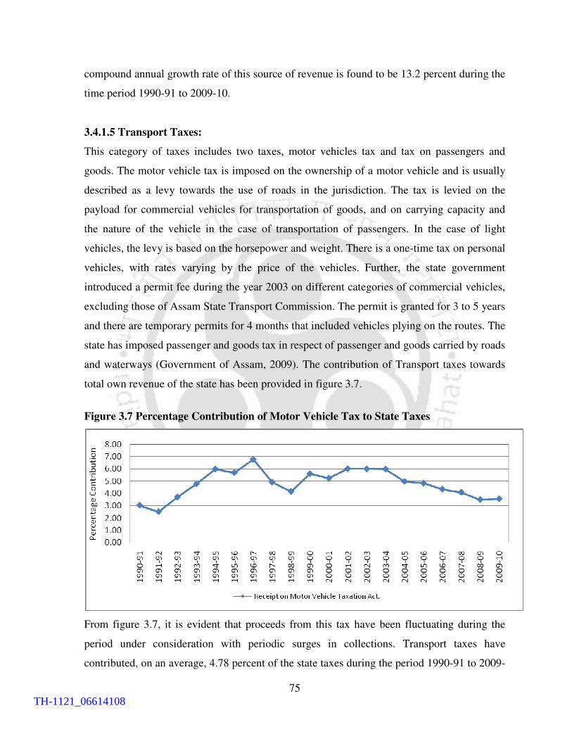
75

compound annual growth rate of this source of revenue is found to be 13.2 percent during the

time period 1990-91 to 2009-10.

3.4.1.5 Transport Taxes:

This category of taxes includes two taxes, motor vehicles tax and tax on passengers and

goods. The motor vehicle tax is imposed on the ownership of a motor vehicle and is usually

described as a levy towards the use of roads in the jurisdiction. The tax is levied on the

payload for commercial vehicles for transportation of goods, and on carrying capacity and

the nature of the vehicle in the case of transportation of passengers. In the case of light

vehicles, the levy is based on the horsepower and weight. There is a one-time tax on personal

vehicles, with rates varying by the price of the vehicles. Further, the state government

introduced a permit fee during the year 2003 on different categories of commercial vehicles,

excluding those of Assam State Transport Commission. The permit is granted for 3 to 5 years

and there are temporary permits for 4 months that included vehicles plying on the routes. The

state has imposed passenger and goods tax in respect of passenger and goods carried by roads

and waterways (Government of Assam, 2009). The contribution of Transport taxes towards

total own revenue of the state has been provided in figure 3.7.

Figure 3.7 Percentage Contribution of Motor Vehicle Tax to State Taxes

From figure 3.7, it is evident that proceeds from this tax have been fluctuating during the

period under consideration with periodic surges in collections. Transport taxes have

contributed, on an average, 4.78 percent of the state taxes during the period 1990-91 to 2009-

TH-1121_06614108

76

10. The receipt on Motor Vehicle Taxation Act experienced a compound annual growth rate

of 14.9 percent during the period 1990-91 to 2009-10.

3.4.1.6 Sales Tax and VAT:

Sales tax revenue in Assam consists of three components, general sales tax act applicable to

local sales, central sales tax applicable on inter-state sales and an entry tax applicable on

selected goods imported into the state from other states in India. In addition to these taxes,

the state also collects luxury tax on the sale of tobacco products and some textiles. The

general sales tax is basically first point tax. Some commodities prone to evasion are taxed at

two points – first point and last point. The government of Assam conforms to the floor rate

regimes agreed upon by all the states in November, 1999. Taxable commodities are

categorized mainly into four rate slabs, 0, 4, 8 and 12. Regarding concessions, there are no

concessions granted for the purchase of raw materials for manufacturing within the state,

except as a part of the industrial incentives package, accessible to new and expanding

industrial units as well as small scale units. Central sales tax is levied on inter state sales, the

maximum rate being 4 percent. The state had also started levying an entry tax from the year

2001. This is levied on the entry of selected goods into the state, intended for consumption or

use by the importing dealer (Government of Assam, 2010). In order to prevent perceived

inconveniences to the local dealers, the entry tax is levied if the goods brought in are not for

resale, thus obviating the need for providing a set-off against taxes on subsequent sales. The

goods covered include sugar and textiles, cereals and motor vehicles. The commodities that

include the bulk of the sales tax revenue to the state are petroleum products, medicines,

motor vehicles, coal gas, coal and coke, tinned and packet food, electronic goods, iron and

steel materials, cement, edible oil and India made foreign liquor (IMFL) etc. Of these goods,

petroleum products contributed over 45 percent of the total sales tax collections in the state

during the year 2001-02 (Government of Assam, 2003). The Government of Assam has

developed a Value Added Tax (VAT) Act, which is being reviewed for ensuring conformity

with the national consensus. The design of the VAT is restricted to goods alone and allows

for a set-off only for taxes paid within the state. In other words, it does not address the

problem of taxation of inter-state trade. Value Added Tax was introduced in the state after a

delay of one month i.e. May 2005 from the date of implementation of VAT throughout the

TH-1121_06614108

77

country i.e. April 2005. The contribution of sales tax towards total own revenue of the state

has been provided in figure 3.8.

Figure 3.8 Percentage Contribution of Sales Tax to State Taxes

It can be inferred from figure 3.8 that, sales tax is the most important source of own tax

revenue for the state as it contributes a major portion of the state’s taxes during the study

period. Average contribution of this source of revenue towards total state taxes is found to be

68.80 percent during the period under consideration. The corresponding figure for all states

average is found to be 59.23 percent during the period of study (RBI, 2011). It implies that

the dependence of the state on sales tax is comparatively more than the average of all states.

As sales tax is the most significant source of tax revenue, it is necessary to examine the

impact of the new structure of sales tax on revenue collection and volatility in the growth

rate. The comparative position of pre-VAT sales tax collection (2000-01 to 2004-05) and

post VAT (2005-06 to 2009-10) tax collection including VAT and growth rate in each of the

years is furnished in table 3.9.

TH-1121_06614108

78

Table 3.9

A Comparative Position of the Pre-VAT and Post-VAT Collection of Sales Tax in the

State (` ` ` ` in crore)

Pre-VAT Post-VAT

Year Actual

Collection

Annual

Percentage of

Growth

Year Actual

Collection

Annual

Percentage of

Growth

2000-01 918 23.72 2005-06 2568 22.34

2001-02 1073 16.88 2006-07 2783 8.37

2002-03 1441 34.30 2007-08 2727 -2.01

2003-04 1551 7.63 2008-09 3111 14.08

2004-05 2099 35.33 2009-10 3535 13.63

Avergae annual growth rate

(2000-01 to 2004-05) 23.57

Avergae annual growth rate

(2000-01 to 2004-05) 11.28

Source: Reports of the Comptroller and Auditor General of India, 2010

Note: Assam Entry Tax not included.

It is clearly evident from table 3.9 that the average growth rate of sales tax during the period

2000-01 to 2004-05 was found to be 23.57 per cent while the growth rate for the period

2005-06 to 2009-10 was 11.28 per cent. Thus, the average growth rate in the post VAT

period registered a decrease of 12.29 per cent implying that implementation of VAT in the

state is not as productive as expected by the government. The decline in the growth rate

during the post-VAT period may suggest that VAT is not beneficial for importing states

where value addition is lower relative to the exporting states. As Assam is a net importing

state, this may imply that not much value addition has taken place in the state. Also, no

improvement has been observed in the volatility of revenue collection in the post-VAT

period. The state even experienced negative growth of sales tax revenue in the year 2007-08.

3.4.1.7 Taxes and Duties on Electricity:

This Act on taxes and duties on electricity provides for levy of duty on the generation and

consumption of electrical energy in the State. The legislative power of the State Legislature

is, however, subject to the restriction imposed by Articles 287 and 288 of the Constitution of

India. The general rate of duty is 5 paise per unit of electricity generated or sold subject to

such concessions as are provided in Section 12 of the Act. The concessional rate of duty is

applicable in respect of industrial consumption only which extends from 1 paise per unit to 3

paise per unit depending on the quantity of energy consumed. The percentage contribution of

this tax has been provided in figure 3.9.

TH-1121_06614108

79

Figure 3.9 Percentage Contribution of Taxes & Duties on Electricity to State Taxes

It is evident from figure 3.9 that taxes and duties on electricity is not a significant source of

revenue for the state government. On an average, it contributes less than one percent of the

state taxes during the period under study.

3.4.1.8 Other Taxes and Duties: The taxes which are not included in the above categories of

taxes experienced a compound annual growth rate of 14.9 percent during the period 1990-91

to 2009-10. These include taxes such as Amusement and betting tax, Luxury tax (Hotels and

Lodging) and Assam Entry tax etc. The contribution of other taxes and duties has been

provided in figure 3.10.

Figure 3.10 Percentage Contribution of Other Taxes and Duties to State Taxes

TH-1121_06614108

80

It can be seen from figure 3.10 that other taxes and duties contributes a significant portion of

the state tax during the study period. On an average, other taxes and duties have contributed

7.89 percent of the state taxes of the government during the period of study. Increase in the

share of other taxes and duties towards own tax revenue of the state government is mainly

contributed by taxes such as Amusement and Betting tax, Luxury tax (Hotels and Lodging)

etc. (Government of Assam, 2010)

3.4.2 State’s Own Non-Tax Revenue:

Own non-tax revenue of Assam comprises of royalty on petroleum, interest receipts,

dividends and profits, and receipts from different general, social, fiscal and economic

services. The contribution of different components of non-tax revenue and their compound

growth rate has been provided in table 3.10.

It is evident from table 3.10 that proceeds from royalty on petroleum are the major

contributor of the non-tax revenue for the study period. On an average, royalty on petroleum

has contributed 75 percent of the total non-tax revenue of the state for the period taken for

analysis. As far as the royalty rates are concerned, the state government can do very little

except persuade the central government to increase the rate from time to time. Proceeds from

interest receipts and dividends and profits have gained their significance during the period of

study. The compound growth rate of interest receipts and dividends and profits is found to be

36.17 and 33.69 percent respectively during the period 1990-91 to 2000-10. Significant

increase in the contribution of interest receipts has been observed during the time period

2004-05 to 2009-10. The increased share of interest receipt during this period is mainly due

to large cash balance of the state government in Reserve Bank of India during that period

(Government of Assam, 2010). The contribution of other sources of non-tax revenue is found

to be insignificant during the study period.

TH-1121_06614108

81

Table 3.10

Contribution of Different Sources of Non-tax Revenue towards Total Non-tax Revenue in Assam (` ` ` ` in lakhs)

Year Interest Receipts Dividends and

Profits General Services Social Services

Fiscal

Services

Economic Services

excluding Petroleum

Petroleu

m Total

1 2 3 4 5 6 7 8 9

1990-91 140 (0.50) 6 (0.02) 774 (2.79) 626 (2.26) – 5442 (19.61) 20765 (74.82) 27753

1991-92 209 (0.80) 23 (0.09) 1624 (6.19) 593 (2.26) – 4397 (17.05) 19405 (73.92) 26251

1992-93 248 (0.54) 9 (0.02) 1363 (2.96) 675 (1.47) – 5380 (11.69) 38376 (83.33) 46051

1993-94 238 (0.68) 8 (0.02) 1934 (5.54)) 675 (1.93) – 6812 (19.52) 25232 (72.30) 34899

1994-95 215 (0.66) 5 (0.02) 1902 (5.83) 611 (1.87) 1 (0.003) 4160 (12.74) 25756 (78.89) 32649

1995-96 244 (0.73) 3 (.01) 2521 (7.51) 681 (2.03) – 4665 (13.90) 25445 (75.82) 33560

1996-97 215 (0.67) 37 (0.11) 1872 (5.81) 641 (1.99) – 5069 (15.74) 24380 (75.68) 32213

1997-98 214 (0.56) 35 (0.09) 3357 (8.81) 665 (1.74) – 3655 (9.59) 30196 (79.21) 38122

1998-99 218 (0.48) 2 (.001) 5811(12.86) 914 (2.02) – 8017 (17.74) 30236 (66.90) 45197

1999-00 247(0.56) 44(0.10) 5204(11.70) 949(2.13) – 6075(13.66) 31973 (71.86) 44492

2000-01 427(0.81) 73(0.14) 4270(8.11) 1154(2.19) – 9949 (18.88) 36804 (69.87) 52677

2001-02 309 (0.58) 83 (0.16) 1698 (3.18) 1323 (2.48) 1 (0.002) 4449 (8.34) 45458 (85.26) 53319

2002-03 307 (0.44) 593 (0.86) 2483 (3.58) 1308 (1.89) 1 (.001) 7323 (10.57) 57283 (82.66) 69296

2003-04 589 (0.62) 688 (0.73) 3435 (3.63) 4996 (5.28) 1 (.001) 12769 (13.50) 72103 (76.23) 94580

2004-05 1006 (0.94) 929 (0.87) 6383 (5.97) 2117 (1.98) – 7980 (7.46) 88587 (82.79) 107001

2005-06 3641 (2.50) 1547 (1.06) 3474 (2.38) 3858 (2.64) – 11790 (8.08) 121616 (83.34) 145927

2006-07 16749 (9.01) 1854 (1) 3274(1.76) 13526 (7.27) – 11942 (6.42) 138582 (74.54) 185927

2007-08 24072 (11.28) 2400 (1.12) 14029 (6.57) 3089 (1.45) – 15080 (7.07) 154788 (75.51) 213458

2008-09 43316(19.07) 1945(0.86) 13977(6.15) 2088 (0.92) – 22852 (10.06) 143012 (62.95) 227189

2009-10 49363 (17.93) 1492 (0.54) 35150 (12.77) 2496 (0.91) – 29376 (10.67) 157418 (57.18) 275295

CAGR (1990-91 to 1999-00) 6.51 24.78 23.58 4.73

6.93 4.91 5.38

CAGR (2000-01 to 2009-10) 69.52 39.83 26.39 8.95

12.78 17.52 20.17

CAGR (1991-91 to 2009-10) 36.17 33.69 22.24 7.55

9.28 11.25 12.84

Source: Directorate of Economics and Statistics, Government of Assam, Various issues

Figures in parentheses represent the percentage contribution of different sources of non-tax revenue towards total non-tax revenue

TH-1121_06614108

82

The above analysis gives an idea about contribution and pattern of own tax and non-tax

revenue of the state. The contribution of the tax and non-tax revenue of the state depends to a

great extent on the revenue effort of the government. The next section of the chapter is

concentrated on the revenue effort of the state government.

3.5 Revenue Effort of the Government of Assam:

Revenue effort may be defined as the difference between revenue potential of the state and

actual collection of revenue. It is basically related to more collection of revenue through

optimum utilization of tax and non-tax bases. The importance of revenue effort lies in the

fact that it leads to enhancement of state’s own revenue in terms of increase in collection of

own tax or non-tax revenue. Apart from that, Central transfers to the state increase

automatically as the tax effort and fiscal discipline are important criterion for inter-state

devolution of central transfers as recommended by the recent Finance Commissions. The

recent Finance Commissions of India namely Tenth, Eleventh, Twelfth and Thirteenth

Finance Commission have given importance to tax effort and fiscal discipline of the states

by assigning due weightage as shown in table 3.4. The Finance Commission of India

measures tax effort as the ratio of per-capita own tax revenue of a state to its per-capita

income. Fiscal discipline is measured by the improvement in the ratio of own revenue receipt

of the state to its total revenue expenditure, related to similar ratio of all states. As own tax

revenue is the main source of total own revenue of the state, increase in tax effort is very

essential for overall fiscal scenario of the state. Tax effort is a process that seeks to mobilize

more revenue as the economy expands and taxable capacity increases (Oommen, 1987). It

takes several forms such as introduction of new taxes, changes in the rates and basis of

existing taxes, improvement in administration etc. Any measure of tax effort has to be related

to taxable capacity. The need to compare tax effort was felt particularly in the context of

fiscal transfers to the states under the various articles of the Constitution; particularly article

275 and 282 (Reddy, 1975). The First Finance Commission was supposed to consider tax

effort as criteria while recommending grants-in-aid under article 275, but was not clearly

indicated by the Commission about the operational technique that was employed by it to

measure the tax effort. The Second Finance Commission too conceded the relevance of tax

effort as a consideration worth keeping in mind, but avoided measuring inter-state tax effort.

TH-1121_06614108

83

The Third Finance Commission did not try to measure the tax potential, on the ground that

determination of inter-state tax effort had to be related to their tax potential and required

special study. The Fourth Finance Commission agreed the principles of considering how far

the state had made efforts to raise resources in relation to their tax potential. It was only in

the report of Fifth Finance Commission that an attempt was made for measurement of tax

effort. The Fifth Finance Commission measure of tax effort is a comprehensive measure of

tax effort. But it ignores the distribution of income (wealth which back it up) which may

differ from state to state. Along with that, the structure of income may differ from state to

state that may affect the relative capacities (Reddy, 1975). Again, it is not clear how actually

the Commissions used the results obtained in determining its award with respect to

devolution of central resources among the states. The Sixth Finance Commission had come

out against the use of tax effort as criteria. It was the Ninth Finance Commission came out

with a specific model for assessment of tax effort of states. The Ninth Finance Commission,

in its report, employed a regression approach derived in a certain manner for making

normative tax revenue projections. Although, it is not easy to find a unique method for

measuring taxable capacity or the tax effort of states, different Finance Commissions and

Planning Commissions adopt a simple measure of tax-GSDP ratio to evaluate tax effort and

assign the required weight in the transfer design (Reddy, 1975). An inter-state comparison of

tax-GSDP ratio gives an idea about the performance of the state in terms of tax effort.

Keeping that fact in mind, an inter-state comparison of the tax-GSDP ratio of Assam with

that of other states and all state average have been made during the time period 1990-91 to

2007-08. An Improvement index has been computed as a percentage change over the

previous sub-period to know the improvement of the state in a particular sub-period

compared to the previous one. A, B and C indicate improvement in the sub-period 1995-00,

2000-05 and 2005-10 compared to the sub-period 1990-95, 1995-00 and 2000-05

respectively. Table 3.11 as provided below gives a comparative picture of the tax-GSDP ratio

of Assam in relation to other general and special category states for four sub-periods taken

into consideration.

TH-1121_06614108

84

Table 3.11

A Comparison of Tax-GSDP ratio of Assam and other States of India during 1990-91 to

2007-08

States Tax - GSDP ratio Improvement Index

1990-95 1995-00 2000-05 2005-08 A B C

Andhra Pradesh 6.79 6.54 7.65 8.11 -3.68 16.97 6.01

Bihar 4.32 4.11 4.89 4.67 -4.86 18.98 -4.50

Goa 7.38 7.01 7.22 8.06 -5.01 3.00 11.63

Gujarat 7.9 7.29 7.25 7.16 -7.72 -0.55 -1.24

Haryana 7.34 6.77 8.24 9.01 -7.77 21.71 9.34

Karnataka 9.04 8.52 9.28 10.61 -5.75 8.92 14.33

Kerala 8.48 8.6 8.68 8.29 1.42 0.93 -4.49

Madhya Pradesh 5.19 5.53 6.75 7.60 6.55 22.06 12.59

Maharashtra 7.26 6.88 7.89 7.97 -5.23 14.68 1.01

Orissa 4.66 4.42 6.1 6.16 -5.15 38.01 0.98

Punjab 7.12 6.3 7.54 7.87 -11.52 19.68 4.38

Rajasthan 5.61 5.59 6.93 7.39 -0.36 23.97 6.64

Tamil Nadu 8.67 8.6 9.12 9.89 -0.81 6.05 8.44

Uttar Pradesh 4.97 4.9 6.04 6.78 -1.41 23.27 12.25

West Bengal 5.69 4.59 4.37 4.62 -19.33 -4.79 5.72

Major States 6.54 6.35 7.14 7.62 -2.91 12.44 6.72

Special Category States

Assam 3.89 3.86 4.92 5.33 -0.77 27.46 8.33

Arunachal Pradesh 0.54 0.74 1.69 2.06 37.04 128.38 21.89

Himachal Pradesh 5.17 5.24 5.66 - 1.35 8.02

Jammu and Kashmir 3.66 3.70 5.60 - 1.09 51.35

Manipur 1.59 1.36 1.66 1.92 -14.47 22.06 15.66

Meghalaya 3.39 3.15 3.42 3.80 -7.08 8.57 11.11

Mizoram 0.69 0.70 1.18 1.88 1.45 68.57 59.32

Nagaland 1.58 1.39 1.38 1.91 -12.03 -0.72 38.41

Sikkim 3.97 5.28 7.61 5.79 33.00 44.13 -23.92

Tripura 2.12 2.19 2.72 3.08 3.30 24.20 13.24

Special Category 3.36 3.43 4.30 5.23 2.08 25.36 21.63

Source: Handbook of Statistics of State Government Finances, Reserve Bank of India, various Issues

Central Statistical Organization, Government of India

It is evident from table 3.11 that the state exhibited better performance in tax-GSDP ratio in

the first decade of the present century compared to the previous decade. In fact, the state

experienced deterioration in the tax-GSDP ratio in the second half of the 1990s compared to

the first half. The performance of the state is found to be poor compared to the other non-

special category states such as Karnataka, Kerala, Maharashtra, Tamil Nadu etc for all the

sub-period considered for the study. Although the ratio is found to be higher than the special

TH-1121_06614108

85

category states as aggregates, but it is found to be less than some special category states such

as Himachal Pradesh and Sikkim etc. As tax-GSDP ratio of the state is found to be poor

compared to the other developed states, it is necessary to find out the reasons behind the low

tax GSDP ratio of the state. It is necessary to examine the efforts on the part of the

government to exploit the revenue potential of the state.

It is very difficult to provide a quantitative measurement of revenue potential and

subsequently prescribe policy suggestion on the basis of it. The buoyancy coefficient of the

state revenue particularly with respect to GSDP is a good statistical tool for measuring

revenue effort of a state. Along with that, arrears of tax and non-tax revenue and cost of

collection of different revenue sources provide an idea about the efficiency of the

administrative machinery of the state. Cost recovery of different services is also considered

as an indicator for measuring revenue effort of the government. So, revenue effort is a multi-

dimensional concept which encompasses all the issues such as buoyancy, cost of collection

of different sources of revenue, arrear of revenue and cost recovered from different services

etc.

3.5.1 Buoyancy of Revenue Sources:

Two factors can give rise to growth in tax or non-tax revenues: (1) the rules or rates of tax or

non-tax can be changed to raise more revenue from the same base or (2) the base on which it

is imposed may grow. The growth of revenue in response to GDP or GSDP can therefore be

broken down into two components: the automatic growth as the base on which the tax or

non-tax is charged grows in relation to GDP, and the growth resulting from discretionary

changes in rates and rules. The combined effect of the above mentioned factors on tax or

non-tax revenue is known as the buoyancy of tax or non-tax revenue of the state. The

simplest method for measuring buoyancy for individual year is to calculate growth rate of the

parameter divided by growth rate of GSDP. The year wise buoyancy coefficients of the own

revenue, own tax revenue and own non-tax revenue of Assam has been provided in table

3.12.

TH-1121_06614108

86

Table 3.12

Year wise Buoyancy Coefficients of Own Revenue, Own tax, Sales tax and Own Non-

tax Revenue of Assam*

Year Own

Revenue

Own Tax

Revenue Sales Tax

Own Non-tax

Revenue

1 2 3 4 5

1990-91 1.59 1.54 0.31 1.66

1991-92 0.95 1.90 1.78 -0.47

1992-93 2.59 0.12 1.01 7.40

1993-94 -0.10 1.14 0.89 -1.50

1994-95 -0.02 0.19 0.66 -0.40

1995-96 0.78 1.04 1.29 0.26

1996-97 0.59 1.12 1.38 -0.50

1997-98 1.88 1.76 -0.20 2.15

1998-99 1.13 0.95 0.69 1.54

1999-00 0.45 0.68 0.96 -0.04

2000-01 2.84 2.70 4.17 3.24

2001-02 2.01 2.66 4.15 0.28

2002-03 1.90 1.77 2.58 2.26

2003-04 1.64 0.78 0.85 4.07

2004-05 1.97 2.41 2.74 1.02

2005-06 2.14 1.71 1.99 3.24

2006-07 1.55 0.87 0.94 3.07

2007-08 0.29 -0.36 -0.33 1.50

2008-09 1.18 1.65 1.09 0.45

2009-10 1.48 1.46 0.98 1.53

Source: Author’s own calculation based on the data on Handbook of statistics of State

Government Finances, Various issues

*Fiscal variables which are used for measuring buoyancy are in current prices. So, GSDP at

current prices are used for computation

It is evident from table 3.12 that the buoyancy coefficients have shown a better performance

in the first decade of the present century than the 1990s. During the year 1992-93, the

buoyancy of non-tax revenue was found to be 7.40, the highest among the period covered for

analysis. The huge increase of non-tax revenue in the above year over the previous year was

mainly due to more collection of cess on indigenous crude oil and other receipt (Government

of Assam, 1993). But for rest of the years in 1990s, the state attained moderate or negative

buoyancy of non-tax revenue. The non-tax revenue of the state has shown better performance

particularly between the time periods 2000-01 to 2009-10. This was mainly due to increased

TH-1121_06614108

87

royalty on petroleum due to rise in international price on crude oil (Government of Assam,

2011).

A wide variation was observed in the buoyancy coefficient of the own revenue of the state

during the period of study. The computed buoyancy coefficient was found to be 1.59, 0.95

and 2.59 in the year 1990-91, 1991-92 and 1992-93 respectively. This was followed by

negative buoyancy in the year 1993-94 and 1994-95. After that, the buoyancy coefficients

were found to be positive for rest of the years implying that growth of GSDP had a positive

impact on own revenue of the state. The buoyancy coefficient of the tax revenue was found

to be positive for most of the years during the time period 1990-91 to 2009-2010. The sales

tax of the state is also taken for analysis as most of own tax revenue of the state is found to

be contributed by sales tax. In other words, sales tax is the major contributor of the total own

tax revenue of the state. The buoyancy of the sales tax of the state during the time period

2000-01 to 2009-10 was found to be comparatively better than the previous decade.

To have a clear idea about the buoyancies of the above taxes, it is necessary to calculate the

coefficients for a longer time period. The above discussed method is not suitable in this case

as it can be heavily influenced by unusually high or low (or negative) measures of buoyancy

for some of the years, and so is the least satisfactory approach. The alternative and most

elegant approach is to regress the log of tax revenue on the log of the base (e.g. GSDP). The

coefficient on the log of the base is a measure of the tax buoyancy (Haughton, 1998). The

buoyancy of state own tax, non-tax revenue and sales tax of the state for the two decade has

been calculated by regressing the variables to GSDP. The results presented in table 3.13.

TH-1121_06614108

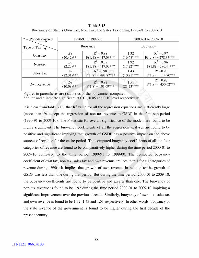
88

Table 3.13

Buoyancy of State’s Own Tax, Non Tax, and Sales Tax during 1990-91 to 2009-10

Periods covered

Type of Tax

1990-91 to 1999-00 2000-01 to 2009-10

Buoyancy Buoyancy

Own Tax .88

(20.42)***

R2 = 0.98

F(1, 8) = 417.03***

1.32

(16.68)***

R2 = 0.97

F(1, 8) = 278.37***

Non-tax .33

(2.23)**

R2 = 0.38

F(1, 8) = 417.03***

1.92

(17.22)***

R2 = 0.96

F(1,8) = 296.44***

Sales Tax .89

(22.31)***

R2 =0.98

F(1, 8) = 497.87***

1.43

(10.71)***

R2 =0.93

F(1,8) = 114.70***

Own Revenue .68

(10.08)***

R2 = 0.92

F(1,8) = 101.69***

1.51

(21.23)***

R2 =0.98

F(1,8) = 450.62***

Figures in parentheses are t statistics of the buoyancies computed

***, ** and * indicate significant at 0.01, 0.05 and 0.10 level respectively

It is clear from table 3.13 that R2 value for all the regression equations are sufficiently large

(more than .9) except the regression of non-tax revenue to GSDP in the first sub-period

(1990-91 to 2009-10). The F-statistic for overall significance of the models are found to be

highly significant. The buoyancy coefficients of all the regression analyses are found to be

positive and significant implying that growth of GSDP has a positive impact on the above

sources of revenue for the entire period. The computed buoyancy coefficients of all the four

categories of revenue are found to be comparatively higher during the time period 2000-01 to

2009-10 compared to the time period 1990-91 to 1999-00. The computed buoyancy

coefficient of own tax, non tax, sales tax and own revenue are lees than 1 for all categories of

revenue during 1990s. It implies that growth of own revenue in relation to the growth of

GSDP was less than one during that period. But during the time period, 2000-01 to 2009-10,

the buoyancy coefficients are found to be positive and greater than one. The buoyancy of

non-tax revenue is found to be 1.92 during the time period 2000-01 to 2009-10 implying a

significant improvement over the previous decade. Similarly, buoyancy of own tax, sales tax

and own revenue is found to be 1.32, 1.43 and 1.51 respectively. In other words, buoyancy of

the state revenue of the government is found to be higher during the first decade of the

present century.

TH-1121_06614108

89

3.5.2 Cost of Collection:

In a underdeveloped economy state like Assam, where optimum collection of revenue is an

important prerequisite of economic development, cost of collection of different taxes play a

very significant role. Minimization of the cost of tax collection is considered to be an

important objective of taxation policy (Ahmed, 1968). But all taxes do not have similar cost

implications. Moreover, a given tax structure implies a certain level of fixed costs, and any

addition to the cost of collection would naturally be determined by the type of changes in the

existing structure. The above mentioned factors have to be taken into consideration while

estimating the cost of collection. It is generally expected that average cost of collection of all

types of taxes falls with increase in total tax yield in a comprehensive manner (Dhawan,

1968). The cost of collection of different taxes and duties of the state has been provided in

table 3.14.

Table 3.14

Cost of Collection of Taxes and Duties in Assam (`̀̀̀ in crore)

Year Gross

Collection

Expenditure

on Collection

Percentage of Expenditure

to Gross Collection for

Assam

Percentage of Expenditure

to Gross Collection for All

States

1 2 3 4 5

1990-91 420 31.58 7.52 5.14

1991-92 512 36.45 7.12 4.71

1992-93 518 36.1 6.97 4.64

1993-94 613 42.6 6.95 4.60

1994-95 632 48.65 7.70 4.33

1995-96 702 53.26 7.59 4.19

1996-97 767 57.48 7.49 4.13

1997-98 882 59.89 6.79 4.11

1998-99 983 67.14 6.83 7.41

1999-00 1225 96.06 7.84 6.41

2000-01 1413 97.06 6.87 6.76

2001-02 1566 92.27 5.89 7.31

2002-03 1935 100.52 5.19 6.49

2003-04 2070 100.33 4.85 6.12

2004-05 2713 159.65 5.88 5.80

2005-06 3232 119.32 3.69 4.28

2006-07 3483 134.63 3.87 3.93

2007-08 3360 133.73 3.98 2.86

2008-09 4039 260.22 6.57 3.04

2009-10 4333(RE) 294 6.78 3.67

Source: Report of Comptroller and Auditor General of India, Government of Assam, various Issues

TH-1121_06614108

90

It is evident from table 3.14, till 1997-98, the cost of collection of taxes as a percentage of

total collection for the state was found to be higher than the all states of India. However, the

all states’ average figure was found to be higher than the state’s figure for most of the years

during 1998-99 to 2005-06. After 2006-07, the cost of collection of taxes and duties for the

state again was found to be higher than the corresponding figure of all states. The cost of

collection of taxes and duties of the state in comparison to all states’ average has been shown

in figure 3.11.

Figure 3.11 Cost of Collection of Taxes and Duties as a percentage of Total Collection

The above analysis shows the cost of collection of different taxes on an aggregate basis. It is

always better if we analyze the cost of collection of major taxes of Assam to that of all India

average. The costs of collection of major taxes in Assam during the period 1990-00 and

2008-09 have been provided in table 3.15.

TH-1121_06614108

91

Table 3.15

Cost of Collection of Different State Taxes during the Time Period 1999-00 and 2008-09

Sl No. Type of Tax Year Gross

Collection

Expenditure

on Collection

Percentage of

Expenditure to Gross

Collection

All India

Average Cost

of Collection

during 2000-09

1 Sales Tax

1999-00 742.32 25.56 3.44

0.83

2000-01 917.89 13.02 1.42

2001-02 1072.76 13.61 1.27

2002-03 1440.90 13.22 0.92

2003-04 1551.06 16.14 1.04

2004-05 2098.58 14.70 0.70

2005-06 2568.41 19 0.74

2006-07 2783.24 34.93 1.26

2007-08 2691.43 23.39 0.87

2008-09 3110.58 39.49 1.27

2 State Excise

1999-00 - - -

3.24

2000-01 137.56 6.49 4.72

2001-02 150.91 7.32 4.85

2002-03 121.67 7.18 5.90

2003-04 - - -

2004-05 - - -

2005-06 - - -

2006-07 174.88 9.70 5.55

2007-08 188.71 10.37 5.50

2008-09 198.68 11.62 5.85

3 Taxes on

Vehicles

1999-00 68.69 4.58 6.67

2.58

2000-01 73.77 5.20 7.05

2001-02 93.59 4.91 5.25

2002-03 116.28 5.21 4.48

2003-04 124 5.29 4.75

2004-05 134.72 6.33 4.70

2005-06 155.91 8.15 5.23

2006-07 151.15 8.08 5.35

2007-08 138.62 8.36 6.18

2008-09 145.21 9.03 6.22

4 Stamps and

registration

1999-00 - - -

2.08

2000-01 38.33 6.82 17.65

2001-02 41.97 5.83 13.89

2002-03 50 6.49 12.98

2003-04 62.12 5.30 8.53

2004-05 - - -

2005-06 - - -

2006-07 97.32 3.91 6.07

2007-08 109.91 6.27 3.71

2008-09 111.17 10.28 9.23

Source: Report of the Comptroller and Auditor General of India, Government of Assam, various

issues

TH-1121_06614108

92

From table 3.15, the cost of collection of different taxes of Assam as measured by the

percentage of expenditure to gross collection is found to be higher than all India figures for

most of the years taken under consideration. The cost of collection of sales tax is found to be

comparatively lower for Assam than other taxes such as State Excise, Taxes on vehicles and

Stamps and Registration. Tax on Stamp and Registration is found to be most expensive in

terms of cost of collection as cost of collection of stamp and registration is higher than all

other taxes taken for the analysis. The cost of collection of stamp and registration was found

to be 17.65 percent in the year 2000-01. But gradually it declined and in the year 2007-08,

the figure came down to 3.71 percent of the gross collection. On a comparative basis, the

taxes on vehicles and stamps and registration exhibit very high cost of collection than the all

India average. This needs to be rectified by enforcing more efficiency in the tax

administrative machinery.

3.5.3 Arrears of Revenue:

Another important indicator of revenue effort is the arrears of own revenue accumulated over

the years. The Finance or Administrative department of the state furnishes the year wise data

on arrears of revenue. Arrears of revenue are defined as the outstanding amount of

uncollected tax and non-tax revenue of the state during a year. This tells about the

inefficiency of the tax administrative machinery of a particular state. The arrears on the

revenue receipt as a percentage of own revenue of the state has been provided in table 3.16.

TH-1121_06614108

93

Table 3.16

Arrears on Revenue Receipt of the State (`̀̀̀ in crore)

Year Arrears of revenue

Receipt

Arrears of Revenue Receipt as

Percentage of Own Revenue Receipt

1 2 3

1992-93 111.17 11.37

1993-94 111.17 11.56

1994-95 137.76 14.36

1995-96 160.50 15.46

1996-97 229.52 21.08

1997-98 208.40 16.50

1998-99 NA* -

1999-00 NA -

2000-01 NA -

2001-02 2784 133.11

2002-03 2757 105.12

2003-04 745 25.54

2004-05 725 19.67

2005-06 768 16

2006-07 755 14.11

2007-08 756 14.32

2008-09 756 12.12

2009-10 722 12.56

Source: Report of Comptroller and Auditor General of India, Government of Assam, various issues

during 1998-2010.

*Finance/Administrative Departments did not furnish year-wise position of arrears of revenue during

1999-2000 to 2001-2002

It is clearly evident from table 3.16 that the state has been incurring huge arrears of revenue

for most the years taken for discussion. However, figures on arrears of revenue for the years

1998-99, 1999-00 and 2000-01 were not made available by the concerned department. There

was a sudden jump in the arrear of revenue in the year 2001-02 and 2002-03. It constituted

around 133.11 and 105.12 percent of total own revenue receipt of the state in the year 2001-

02 and 2002-03 respectively. After that, there was sudden decline of the arrears of revenue in

the year 2003-04 when it constituted 25.54 percent of the total revenue compared to 133.11

and 105.12 percent in the year 2001-02 and 2002-03 respectively. In other words, the

government was able to collect revenue amounting to 2012 crore as an arrear in the year

2003-04. This signifies the importance of the administrative machinery for proper fiscal

management. The improvement in the administrative machinery was particularly due to

introduction of computerization of tax administrative machinery in the state. The “Fiscal

TH-1121_06614108

94

Reform Facility” as adopted by the Government of Assam also forced the government to

tighten the tax or non-tax administrative machinery. The report of the Comptroller and

Auditor General of India in their report on 31 March, 1999 pointed out that Finance and

Administrative Department did not furnish the figures on arrears and there was huge arrears

of state’s revenue. All the above factors forced the government to take immediate measures

for reduction of arrears. But in spite of measures to reduce inefficiency in revenue collection,

the arrears of revenue still constitute 12.56 percent of the total own revenue of the state. The

arrears of revenue of the state as s percentage of total own revenue has been shown in figure

3.12.

Figure 3.12 Arrears of Revenue as a percentage of Own Revenue of the State

It is clearly seen from figure 3.12 that arrear of revenue constitutes a major portion of the

state’s own revenue over the study period. A sharp increase in the in the arrear of revenue

was observed in the year 2001-02 and 2002-03 followed by decline in the subsequent years.

3.5.4. Cost Recovery of Social and Economic Services:

An important indicator of revenue effort is the cost recovery of different social and economic

services provided by the governments. Cost recovery on account of public services has been

a critical issue for state finances (RBI, 2011). The cost recovered from different social and

economic services of the state depends upon various factors such as appropriate user charges,

proper effort of the administrative machinery etc. It is measured as a ratio of revenue receipts

from a particular service to non-plan revenue expenditure incurred on that service. The cost

TH-1121_06614108

95

recovery of social and economic services of Assam vis-à-vis all states has been shown in

table 3.17.

Table 3.17

Cost Recovery of Social and Economic Services of Assam and all States

Year Assam All States Assam All States

Social Services Economic Services

1990-91 1.15 2.61 19.58 33.29

1991-92 0.89 3.13 11.36 25.60

1992-93 1.01 3.05 15.86 32.32

1993-94 0.85 2.97 20.64 32.08

1994-95 0.76 2.82 10.26 34.18

1995-96 0.73 2.70 8.42 33.46

1996-97 0.63 2.69 12.32 26.13

1997-98 0.62 3.31 8.60 24.99

1998-99 0.73 2.84 15.02 26.38

1999-00 0.63 2.96 9.69 30.71

2000-01 0.61 2.84 13.99 24.48

2001-02 0.74 3.11 6.40 26.57

2002-03 0.66 3.29 10.86 29.59

2003-04 2.02 3.58 12.42 25.45

2004-05 0.66 3.67 6.25 38.08

2005-06 1.33 4.18 7.80 31.53

2006-07 3.63 5.78 8.11 30.95

2007-08 0.76 5.86 8.52 30.51

2008-09 0.38 3.91 12.29 31.04

2009-10 0.58 3.47 8.17 32.29

Source: State Finances: A study of Budgets, Reserve Bank of India, Various issues

It has been observed that cost recovered from various social and economic services in Assam

is much lower than the all states average during the period of study. No improvement in the

performance of the state has been observed during the period of study implying that there is a

need for rationalization of the user charges on different social and economic services of the

state. The cost recovered from social services is found to be lower than cost recovery of

economic services for the state as well as for all states. The recovery rate of social and

economic services of the state in comparison to all states has been shown in figure 3.13 and

3.14.

TH-1121_06614108

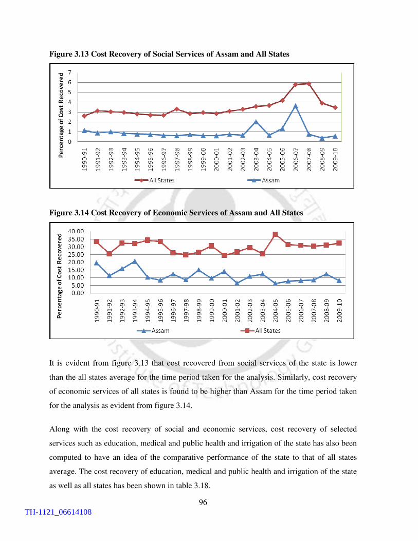
96

Figure 3.13 Cost Recovery of Social Services of Assam and All States

Figure 3.14 Cost Recovery of Economic Services of Assam and All States

It is evident from figure 3.13 that cost recovered from social services of the state is lower

than the all states average for the time period taken for the analysis. Similarly, cost recovery

of economic services of all states is found to be higher than Assam for the time period taken

for the analysis as evident from figure 3.14.

Along with the cost recovery of social and economic services, cost recovery of selected

services such as education, medical and public health and irrigation of the state has also been

computed to have an idea of the comparative performance of the state to that of all states

average. The cost recovery of education, medical and public health and irrigation of the state

as well as all states has been shown in table 3.18.

TH-1121_06614108

97

Table 3.18

Cost Recovery of Irrigation, Education and Public Health of the State and all States

Year Assam All States Assam All States Assam All States

Irrigation Education

Medical and Public

Health

1990-91 0.93 - 0.47 1.28 2.76 5.79

1991-92 0.97 - 0.43 1.22 1.99 6.35

1992-93 0.59 - 0.31 1.31 2.83 5.79

1993-94 0.65 - 0.23 1.12 2.86 6.78

1994-95 0.75 - 0.22 1.11 2.56 5.86

1995-96 0.57 9.79 0.24 1.09 1.98 5.17

1996-97 0.33 8.04 0.22 1.01 1.66 4.71

1997-98 0.68 5.95 0.18 1.25 1.97 5.73

1998-99 0.21 6.43 0.20 0.99 2.89 5.07

1999-00 0.65 6.14 0.16 1.32 3.14 5.30

2000-01 0.20 8.12 0.15 1.25 2.62 4.72

2001-02 0.29 7.53 0.20 1.25 4.41 6.29

2002-03 0.44 8.38 0.19 1.61 3.62 5.54

2003-04 0.26 15.29 1.95 1.76 2.06 4.86

2004-05 0.33 16.36 0.24 2.12 1.79 6.17

2005-06 0.17 14.48 1.24 2.82 1.27 4.53

2006-07 0.23 14.95 4.87 2.64 1.19 4.91

2007-08 0.24 15.55 0.22 2.78 1.44 4.78

2008-09 0.19 15.83 0.19 1.63 0.81 6.17

2009-10 0.17 15.15 0.18 1.61 0.74 4.67

Source: Handbook of Statistics of State Government Finances, Reserve Bank of India,

various Issues

It is evident from table 3.18 that cost recovery of irrigation in the state is much lower than the

all state average for the time period considered for the analysis. Similarly, the cost recovery

of medical and public health of the state is found to be less than all states average for the

study period. The cost recovery of education of the state is lower than all states average

except in the year 2003-04 and 2006-07. The cost recovery of these selected services of the

state as well as all states has been provided in figure 3.15, 3.16 and 3.17.

TH-1121_06614108

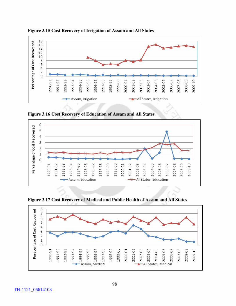
98

Figure 3.15 Cost Recovery of Irrigation of Assam and All States

Figure 3.16 Cost Recovery of Education of Assam and All States

Figure 3.17 Cost Recovery of Medical and Public Health of Assam and All States

TH-1121_06614108

99

It is evident from figure 3.15, 3.16 and 3.17 that cost recovery of selected services of the

state is much less than all states average. Urgent steps are required on the part of the

administrative machinery for realisation of larger revenue from these services through

appropriate user charges.

The above discussion gives an idea about the efforts of the state government to mobilise

more revenues. As discussed in the previous sections, revenue effort of the government

depends upon revenue potential of the government which in turn is determined by growth of

GSDP of the state. Under these circumstances, it is necessary to study the impact of the

GSDP and other relevant factors on the revenue effort of the government which is carried out

in the next section.

3.6 Panel Regression Analysis of Revenue Effort of the State Government:

It may be recalled that some broad conclusions regarding revenue effort of the government

were drawn from the previous discussions as indicated by the simple tools such as ratios,

averages, etc. But these conclusions based on ratios, averages, etc. may not be rigorous

enough and may sometime be misleading too. This is due to the fact that while comparing

averages and ratios, other influencing factors are not necessarily kept constant or controlled.

The apparent differences in averages or ratios, therefore, may be because of configuration of

values of other factors. To be able to draw inferences in a more rigorous manner, a two-

variate panel regression analysis has been carried out to analyze the impact of the relevant

variables on revenue effort of the state. Panel models are considered to perform better than

the conventional models based on a single dimension of either time-series or cross-section of

data as panel data techniques controlled for those relevant variables along time as well as

cross section dimensions. In these models, the substantial increase in degrees of freedom

helps to increase the reliability of estimates. Further, the quality of the parameter might be

better as the pooled sample permits the incorporation of specificities of individual groups or

states in the model (Wooldridge, 2007).

In this model, per-capita own tax revenue (Y) is used as a proxy for overall revenue effort

of the government. Non-tax revenue is not considered for this regression model as non-tax

TH-1121_06614108

100

revenue of the government is mainly contributed by royalty on petroleum which in turn

depends on the international prices on crude oil. The royalty on petroleum, on an average,

has contributed 75 percent of the total non-tax revenue of the state government. The

contribution of the other sources of non-tax revenue is found to be insignificant during the

period of study. In other words, major portion of the non-tax revenue is found to be

independent of revenue effort of the government. Considering the above fact, per-capita own

tax revenue is taken as a dependent variable of the model.

Available literature on revenue effort has identified various relevant variables which have an

impact on revenue generation of the state government such as GSDP, rate of urbanization,

literacy rate and revenue expenditure of the previous year etc. As year wise data on

urbanization and literacy rate are not available for all the states, these two variables are not

considered for the analysis. The explanatory variables which have been considered initially

for the analysis are given below:

i. Per-Capita GSDP (X1): GSDP is considered to be main determinant of the tax revenue

of a government. An increase in GSDP is expected to increase the tax revenue of the state

government if proper effort is put up by the government. In this regression model, GSDP

is considered in terms of per-capita basis as states with higher per-capita income have

more revenue potential with same level of GSDP. Considering the above fact, the

Finance Commissions of India also use per-capita GSDP as a proxy for revenue potential

while measuring the tax effort of the state governments.

ii. Per-capita Revenue Expenditure of the Previous Year (X2): Another variable, per-

capita revenue expenditure of the previous year is also considered to observe the sense of

urgency of the state government to control revenue expenditure for fiscal stability. It also

represents the state’s fiscal situation and the need for augmenting resources. Available

literature on government finances states that excessive increase in revenue expenditure is

one of the reasons for fiscal imbalances. High revenue expenditure in the previous year

should generally compel the states to augment revenue in the current year. This indicates

the demand side of increasing the tax effort (Panda, 2009).

TH-1121_06614108

101

The time period taken for the analysis was from 1990-91 to 2009-10. To have a comparative

analysis with other states, 15 major states have been considered along with Assam. Data on

Gross Domestic Product of the states at current and constant prices in the series 1980-81,

1993-94, 1999-00 and 2004-05 are obtained from the Central Statistical Organization. All the

data are converted into 2004-05 prices by splicing to make it comparable with the above

mentioned series. Mid-year population figures have been taken from CSO and price deflators

have been computed from the ratio of current to constant price GSDP figures. This is used to

convert the fiscal data into constant price term (with 2004-05 prices as base) and per-capita

term whenever necessary. On initial estimation of the model, the value of the coefficient of

the variable ‘revenue expenditure of the previous year’ has come out positive as expected but

insignificant. Therefore, to facilitate better treatment of the model, the analysis has been

reworked by dropping the above variable. Thus, a panel regression analysis is constructed as

follows:

Yit = α0 + α1 Xit + uit................................ (1)

Here,

Y is the per-capita own tax revenue of the states.

X is the per capita GSDP of the states.

i stands for the ith

cross sectional unit and t for the tth

time period.

u is random disturbance or error term.

α0 and α1 are the parameters to be estimated in the model.

To decide between fixed or random effects, Hausman test is used where the null hypothesis is

that the preferred model is random effect versus the alternative the fixed effect (Greene,

2008). By applying this test, it has been ascertained that a random effect model will be more

appropriate for the present data set. Accordingly, the panel regression analysis has been

carried out by applying random effect model. Presence of autocorrelation and

heteroscedascity has been checked by using Pearson cross sectional dependence test and

Modified Wald test for group wise heteroscedasticity respectively. The panel regression is

estimated by using the econometric software STATA 11. The results of the panel regression

are provided in table 3.19.

TH-1121_06614108

102

Table 3.19

Results of the Random Effect Model on Revenue Effort of the Government

Variables Estimated

Coefficients t-statistic

Per- capita GSDP .0849279

(.001582)*** 53.68

Constant -244.2238

(74.05468)*** -3.30

Hausman test

(p-value)

0.4873***

(.000531)

Wald chi2 2881.80***

R2 within 0.8946

R2 between 0.9561

R2 overall 0.9395

Figures in parentheses represent standard error of the estimated coefficients

***, ** and * indicate significant at 0.01, 0.05 and 0.10 level respectively

The value of the coefficient of determination (R2) of the model is found to be very high

suggesting a good fit of the model. The coefficient estimates obtained from the above panel

data model reflects the average relationship across states. It implies that, on an average, 8.5

percent of the per capita GSDP has been mobilised by the states governments as tax revenue

during the period under study. However, to evaluate the performance of Assam in relation to

the other Indian states, the errors have been estimated as the difference between the observed

and estimated values of ‘per capita own tax revenue’ of the state. The estimated errors for the

state for the period under study are presented in table 3.20.

TH-1121_06614108

103

Table 3.20

Calculated Values of the Estimated Errors for the State

Year

Actual Per Capita

Own Tax Revenue

(1)

Fitted Per Capita

Own Tax Revenue

(2)

Estimated Error

(1-2)

1990-91 503 958 -456

1991-92 559 983 -424

1992-93 515 969 -454

1993-94 546 989 -443

1994-95 490 1001 -510

1995-96 497 1006 -508

1996-97 508 1013 -505

1997-98 534 1013 -479

1998-99 519 989 -470

1999-00 570 1011 -441

2000-01 631 1028 -397

2001-02 678 1036 -359

2002-03 778 1092 -314

2003-04 799 1153 -354

2004-05 965 1181 -216

2005-06 1051 1204 -153

2006-07 1074 1249 -175

2007-08 975 1292 -317

2008-09 1069 1363 -294

2009-10 986 1471 -485

It has been found from table 3.20 that the error terms for the state are negative for all the

years taken for the analysis. It implies that Assam has been underperforming as compared to

the other (average) states during the period taken for the analysis. Thus, it suggests that state

has to put more effort for mobilization of additional revenue.

3.7 Composite Index of Resource Mobilisation:

From the above discussion, it is clear that a single indicator of revenue is not sufficient to

assess the overall revenue scenario of the state. For a particular year, the state may perform

well in one aspect, but in rest of the aspects, the performance may not be satisfactory. The

TH-1121_06614108

104

current approach to study the revenue pattern of a state is to use either a single or couple of

ratios relating to different aspects of revenue. Such an approach is too simplistic and does not

encompass all aspects of revenue mobilisation. The revenue mobilization index is the

combination of the important dimensions of the revenue scenario of the state. Considering

the above aspect, a composite index of revenue has been computed on the basis of the

following parameters –

(a) Own Tax-GSDP ratio.

(b) Non-tax-GSDP ratio.

(c) Own Resources-Revenue Receipt ratio.

(d) Real Per-capita Revenue Receipt.

The methodology adopted for construction of the index is same as for the Human

Development Index of UNDP. In all the parameters no normal or goal post value has been

defined. The observed maximum value of the parameters during the study period has been

taken as the maximum or goal post value. As, geometric mean is used for aggregation,

natural zeros are used as a minimum value of the parameters.

The dimension of each parameter is expressed by applying the following formula.

Actual Value - Minimum ValueDimension Index =

Maximum Value - Minimum Value

From the above dimension index, it is clear that the year in which the performance of the

state is found to be maximum gets the highest value of 1. But as natural zeros are used as

minimum values, the year in which the state’s performance is found to be the worst, gets the

minimum value which is greater than 0. The dimension index for each of the parameter has

been computed by applying the above formula. The dimension indices for real per-capita

revenue receipt, ratio of own revenue to total revenue, own tax to GSDP and non-tax to GSDP are

TH-1121_06614108

105

represented by D1, D2, D3 and D4 respectively. The computed revenue mobilization index has

been given in table 3.21.

Table 3.21

Resource Mobilization Index of the State for the Period 1990-91 to 2009-10

Year

Real Per-capita

Revenue

Receipt (in `)

Own

revenue/Total

Revenue

Own

tax/GSDP

Non-

tax/GSDP D1 D2 D3 D4 RMI

1 2 3 4 5 6 7 8 9 10

1990-91 2089 0.236 0.032 0.021 0.334 0.830 0.584 0.700 0.580 1991-92 2605 0.212 0.035 0.018 0.416 0.743 0.638 0.594 0.585 1992-93 2535 0.198 0.032 0.028 0.405 0.696 0.586 0.943 0.628 1993-94 2924 0.185 0.033 0.019 0.467 0.649 0.615 0.634 0.586 1994-95 2271 0.213 0.030 0.015 0.363 0.749 0.547 0.513 0.525 1995-96 2361 0.208 0.030 0.014 0.377 0.730 0.549 0.476 0.518 1996-97 2517 0.199 0.030 0.013 0.402 0.698 0.554 0.422 0.506 1997-98 2587 0.204 0.032 0.014 0.413 0.716 0.587 0.460 0.532 1998-99 2366 0.218 0.032 0.015 0.378 0.766 0.584 0.487 0.536 1999-00 2261 0.253 0.035 0.013 0.361 0.888 0.636 0.418 0.541 2000-01 2525 0.251 0.038 0.014 0.403 0.880 0.694 0.469 0.583 2001-02 2585 0.263 0.040 0.014 0.413 0.922 0.739 0.456 0.598 2002-03 2736 0.285 0.044 0.016 0.437 1.000 0.806 0.523 0.655 2003-04 2999 0.267 0.043 0.020 0.479 0.936 0.791 0.655 0.694 2004-05 3535 0.273 0.051 0.020 0.565 0.958 0.934 0.667 0.762 2005-06 3929 0.268 0.054 0.025 0.628 0.942 1.000 0.818 0.834 2006-07 4225 0.255 0.054 0.029 0.675 0.895 0.989 0.957 0.869 2007-08 4460 0.219 0.047 0.030 0.713 0.770 0.869 1.000 0.831 2008-09 6259 0.173 0.050 0.028 1.000 0.608 0.914 0.921 0.846 2009-10 5806 0.175 0.044 0.022 0.928 0.613 0.800 0.736 0.761

Source: Calculated by the author (basic data from various issues of Handbook of Statistics of State

Government Finances, Reserve Bank of India and CSO reports)

From table 3.21, the value of the index is found to be comparatively less during 1990s than

the first decade of the present century. Gradual improvement of the index has been observed

during the first half of the present decade of the twenty-first century. The performance of the

state is found to be high during the time period 2004-05 to 2009-10. In fact, the state has

achieved maximum value amounting to .869 in the year 2006-07 followed by .830 and .845

in the year 2007-08 and 2008-09 respectively. This result confirms improvement in revenue

mobilization of the state in the first decade of the present century compared to the previous

decade.

TH-1121_06614108

106

3.8 Conclusion:

The foregoing analysis has established the fact that the state is heavily dependent on the

central transfers. The ratio of own revenue to total revenue of the state is found to be

comparatively low than the other developed states and all states average. The state has not

been able to improve the ratio during the period under study. In other words, own revenue

generation of the state is not adequate and the state has to depend on the central transfers for

major part of the developmental activities.

Among the central transfer, grants-in-aid are found to be the major contributor of the total

revenue followed by the shared taxes. The increased contribution of grants-in-aid is the result

of declaration of the state as a special category state. This initiative by the central

government has helped the state to receive more grants from the Planning Commission.

Regarding shared taxes, the introduction of the efficiency factors by the Finance Commission

in their devolution formula has incentivized the state government to bring more efficiency in

revenue collection.

The own tax revenue of the state is basically contributed by the proceeds from the sales tax.

Dependence of the state on sales tax is found to be comparatively higher than all states

average during the period of study. The introduction of VAT is not found to be as effective as

expected. Although, no decline of revenue is noticed after introduction of VAT, but average

growth rate of sales tax in the post VAT period registered a decrease of 9.66 percent in the

first three years compared to the previous three years. The non-tax revenue of the state is

found to be totally dependent on royalty on petroleum. But the royalty on petroleum is in turn

dependent on the international price on crude oil. The contribution of other sources of non-

tax revenue is found to be minimal during the period of study.

Both own tax and non-tax revenue of the state have achieved a higher buoyancy in the first

decade of the present century compared to the previous decade. The non-tax revenue of the

state has maintained very high buoyancy during the time period of 2000-01 to 2009-10. It

implies that growth of GSDP has a positive and significant impact on own revenue of the

state in recent years. But increased arrear of revenue is an area of concern for the state

government. The large arrear of revenue in the later part of 1990s implies inefficiency of tax

TH-1121_06614108

107

administrative machinery. The average costs of collection of different taxes of the state are

also found to be higher than the all India average. The cost recovery of social and economic

services of the state is found to be much lower than all states average. Similarly, cost

recovery of irrigation, medical and public health of the state has been much lower than the all

states average. The cost recovery of education is also found to be low for the state than all

state average for most of the years considered for the analysis. In other words, there is scope

for improvement of the revenue administrative machinery.

The panel regression analysis implies that Assam has been underperforming as compared to

the other (average) states during the period taken for the analysis. The value of the revenue

mobilization index is found to be relatively better during first decade of the present century

compared to the previous decade. Overall, the revenue scenario of the state is found to be

satisfactory in recent years. But it is necessary to examine whether improvement in the

revenue scenario of the state is sufficient enough to discharge the state’s expenditure

responsibilities.

Note:

1. The Gadgil formula was formulated during Fourth Five Year Plan for distribution of

plan transfers amongst the states. It was named after the then Deputy Chairman of the

Planning Commission, Dr. D R Gadgil.

***

TH-1121_06614108

108

TH-1121_06614108

109

Chapter 4

Pattern of Public Expenditure and Expenditure Implications of

Fiscal Reform Measures

In the previous chapter, the nature and pattern of revenue scenario of the state is analysed for

examining the availability of funds for expenditure needs of the state. Improvements have

been noticed in the revenue scenario of the state during the first decade of the present century

compared to the previous decade. The improved revenue scenario of state government is

found to be mainly due to increase in own revenue collection and higher allocation from the

central government. The fiscal reform measures adopted during the time period are found to

be one of the main reasons which has helped the state government to receive more funds

from the central government as well as to increase the state’s own revenue collection. As

fiscal reforms encompass both the aspects of revenue and expenditure, it is necessary to

examine the impact and implication of those expenditure reform measures on pattern and

quality of government expenditure. At the same time, it is also pertinent to study whether

improvements in the revenue scenario of the state are sufficient to discharge the expenditure

responsibilities of the state.

Availability of fund or lack of it for different expenditure obligations actually determines the

economic growth and development of a state. Available literature on public expenditure

states that there is a close relationship between growth of GSDP and growth of public

expenditure (Wagner, 1983; Peacock and Wiseman, 1961; Musgrave, 1969). Mention may be

made of Wagner’s hypothesis which states that an increase in GSDP leads to more than

proportionate increase in public expenditure. In other words, higher public expenditure is a

result of economic growth. In Federal forms of government, states as sub-national level

entities have a vital role in economic development of a country. State governments in India

have to incur different kinds of expenditure either for the satisfaction of the collective needs

of the citizens or for promoting their economic and social welfare. The minimal function of

the state governments in India is to address the problem of market failure and to improve

equity among the people (Gupta, 2001; Dholakia and Dholakia, 2004). Governments have to

undertake those activities where market cannot provide maximal outcome such as providing

TH-1121_06614108

110

pure public goods, maintaining law and order and property rights, providing public health

care facilities and macroeconomic management etc. It is also necessary to improve equity

among the people through such activities such as anti-poverty measures, disaster relief and

public distribution etc. (World Bank, 2005; Government of India, 2002). As public

investment is the main instrument of economic development in India, it is necessary to

analyse the specific expenditure responsibilities of each tier of government.

4.1 Expenditure Responsibilities of the States and Central Government in India:

The Constitution of India has assigned specific expenditure responsibilities to each tier of the

Government under separate list. The Seventh Schedule (Article 246) of the Constitution lays

down the respective financial resources of the Union and State governments in India. It has

been found that most of the developmental and normal administrative functions such as

public order, police, local government, public health and sanitation, hospitals and

dispensaries, agriculture, water, fisheries, public debt etc. are assigned to the states, which

increase their expenditure obligations relative to the Union Government (Heller and Rao,

2006). The responsibility of the central government is to provide the national public goods

such as defence, atomic energy and mineral resources, foreign affairs, diplomatic relations,

railways, airways, posts and telegraph, and currency and coinage etc. In other words, state

governments in India have to play a significant role in a number of areas critical for

enhancing growth and development of the state. They have the responsibility of both

maintaining law and order and providing most of the economic and social infrastructure.

They are closer to the people and have direct interface with them which makes them prone to

comments on governance, quality of expenditure, applications of resources and performance

of the services provided (Lahiri, 2000; Shariff et al. 2002). As a result, proper allocation and

prioritisation of the expenditure of the state governments have been an issue of discussion in

recent times. This is more significant in a state like Assam where public investment plays a

significant role in economic development. Due to its difficult geographical terrain and poor

infrastructure, private sectors are not willing to invest in the state. State government through

its investment on social and physical infrastructure has to remove those bottlenecks that

hinder the development of the state. At the same time, state government has to judiciously

use its limited resources to maintain fiscal stability. The growth of public expenditure on

TH-1121_06614108

111

priority sectors is expected to lead the state in to the path of economic development. Under

these circumstances, it is necessary to analyse the trend and pattern of public expenditure of

the state during the period under consideration.

4.2 Trend and Pattern of Total Expenditure of the State:

Total expenditure of the state includes revenue expenditure, capital outlay and loans and

advances provided by the state government for different activities. The trend and buoyancy

of the total expenditure during the study period provides vital information about the growth

of total expenditure with respect to overall growth of the economy. The ratio of total

expenditure to GSDP has been computed to observe the relative growth of expenditure with

respect to GSDP of the state. As done in the previous chapter, decade wise compound growth

rate has been computed to have an idea about the relative growth of total expenditure in the

two decades. The growth and buoyancy of total expenditure and ratio of total expenditure

with respect to GSDP of the state during the study period has been provided in table 4.1.

TH-1121_06614108

112

Table 4.1

Pattern of Growth and Buoyancy of Total Expenditure of the State during 1990-91 to 2009-10

(`̀̀̀ in crore)

Year Total

Expenditure

Annual Growth of

Total Expenditure

Total Expenditure as a

Percentage of GSDP

Buoyancy of Total

Expenditure

1 2 3 4 5

1990-91 2350

- 17.77 -

1991-92 2678

13.96 18.16 1.10

1992-93 2828

5.59 17.41 0.50

1993-94 3305

16.89 18.04 1.18

1994-95 3679

11.30 17.32 0.72

1995-96 4036

9.72 17.18 0.86

1996-97 3938

-2.44 15.49 *

1997-98 4477

13.69 16.22 1.80

1998-99 4856

8.47 15.70 0.64

1999-00 6461

33.05 18.25 2.68

2000-01 7196

11.37 19.23 2.00

2001-02 7442

3.42 19.11 0.84

2002-03 7749

4.13 17.56 0.31

2003-04 9199

18.72 19.13 2.08

2004-05 13384

45.49 25.06 3.53

2005-06 11727

-12.38 19.75 *

2006-07 12990

10.77 20.08 1.21

2007-08 14575

12.20 20.51 1.24

2008-09 16705

14.61 20.57 1.02

2009-10 23960

43.43 25.91 3.14

CAGR

1990-91 to 1999-00

11.89 - - -

CAGR

2000-01 to2009-10 14.30 - - -

CAGR

1990-91 to 2009-10 13 - - -

Source: Handbook of Statistics on State Government Finances, Reserve Bank of India, various issues

State Finances: A Study of Budgets, Reserve Bank of India, various issues

* Growth of total expenditure is negative in those years

It is clear from table 4.1 that total expenditure of the state government has increased from `

2350 crore in 1990-91 to ` 23960 crore in the year 2009-10 and registering a compound

annual growth rate of 13 percent during that period. This rate, however, is lesser than the

compound growth rate of total expenditure of all states during the same period (14.01 percent

TH-1121_06614108

113

as per RBI, 2011). Similarly, the aggregate expenditure of the government has increased

from ` 2689 crores in 1990-91 to ` 24968 crores in 2009-10 and thus registering a growth

rate of 12.44 percent during that period. The average ratio of aggregate expenditure to GSDP

of the state during the study period is found to be higher compared to the ratio in 1980s (RBI,

2011). The growth rate of total expenditure of the state in the second sub-period (2000-01 to

2009-10) is found to be much higher than the growth rate of total expenditure in the first sub-

period under consideration. While the annual compound growth rate of total expenditure in

2000-01 to 2009-10 was 14.30 percent, the same was found to be 11.89 percent in the

previous sub-period. Additionally, a wide fluctuation has been noticed in the annual growth

rate of total expenditure during the study period. High and unusual increase in total

expenditure of the state has been noticed in some years such as 1999-00, 2004-05, and 2009-

10. The significant increase in total expenditure in 1999-00 and 2009-10 was mainly due to

implementation of the revised pay scale to the government employees. The significant

increase in total expenditure in 2004-05 was due to increase in non-plan revenue expenditure

by ` 1187 crore and capital expenditure under economic services by ` 1545 crore which

were nearly 36 percent and 46 percent respectively of the net increase of total expenditure

over the previous year (Government of Assam, 2005). The state also experienced negative

growth of total expenditure in the year 1996-97 and 2005-06. Decline in revenue expenditure

on economic services and grants-in-aid as well as decline in capital expenditure on general

services contributed towards negative growth of total expenditure in the year 1996-97. The

negative growth of total expenditure in the year 2005-06 was mainly due to decrease in non-

plan capital expenditure by ` 1333 crore and less disbursement of loans by ` 869 crore over

the previous year (Government of Assam, 2005). It is necessary to unearth the reasons for

these fluctuations in total expenditure of the state. The classification of the total expenditure

into different components provides the reasons for such wide fluctuation in total expenditure

which is carried out in the next sub-sections. The average ratio of total expenditure to GSDP

of the state during the period of study is found to be 20.53 percent which is higher than the

ratio in 1980s (which was only 18.84 percent). The total expenditure-GSDP ratio of the state

was found to be more or less stable during 1990s which ranged from 15.70 percent in 1998-

99 to 18.25 percent in 1999-00. After that, the ratio was found to increase and attained a high

of 25.06 percent in 2004-05 which was followed by decline in the subsequent years. A

TH-1121_06614108

114

sudden increase in the ratio was observed in the year 2009-10 as total expenditure-GSDP

ratio of the state jumped from 20.57 percent in 2008-09 to 25.91 percent in 2009-10. As

discussed above, this was due to payment of revised pay scale to the government employees

which led to sudden increase in total expenditure. During the first decade of the present

century, the average ratio of total expenditure-GSDP of the state was found to be

comparatively higher than the previous decade. The year wise buoyancy of total expenditure

of the state has been found to be positive and more than one for most of the years implying

that there was a significant increase in total expenditure with respect to growth of GSDP

during the study period. The total expenditure-GSDP ratio of the state during the period of

study has been provided in figure 4.1.

Figure 4.1 Ratio of Total Expenditure to GSDP of the State during the Study Period

It is evident from figure 4.1 that, during 1990s, the ratio was within the range of 15.70

percent in 1998-99 to 18.25 percent 1990-00. Increase in the ratio was noticed during the

time period 2000-01 to 2009-10, particularly in the year 2004-05 and 2009-10. As increase in

total expenditure has been observed during the period of study, it is necessary to unearth the

reasons for such increase in expenditure during the period under study. The pattern of public

expenditure over the years gives detail information regarding the nature and composition as

well as reasons for increase in expenditure of the state.

4.3 Pattern of Total Expenditure in Assam:

The pattern of expenditure basically implies the allocation of expenditure under different

heads such as revenue expenditure, capital outlay and disbursement of loans and advances

TH-1121_06614108

115

etc. Capital outlay represents net of capital expenditure after repayment of public debt (RBI,

2007). Capital outlay is that part of capital expenditure which is actually spent for creation of

assets. The composition of total expenditure in Assam in terms of revenue expenditure,

capital outlay and disbursement of loans and advances has been provided in table 4.2.

It is quite evident from table 4.2 that revenue expenditure constitutes the major portion of the

total expenditure of the state during the period of study ranging from 80.21 percent in 1991-

92 to 92 percent in 2001-02. On an average, revenue expenditure has constituted 87.86

percent of the total expenditure of the state during the period under study. Compared to that,

revenue expenditure of all states has constituted, on an average, 84.55 percent of the total

expenditure for the above mentioned period (RBI, 2011). The higher proportion of revenue

expenditure to total expenditure of the state compared to all states average implies that fewer

resources are available for other productive uses such as capital outlay and advancement of

loans and advances. This may hamper the overall economic development of the state.

Similarly, capital outlay is found to constitute, on an average, 9.01 percent of the total

expenditure of the state compared to all states average of 11.52 percent during the period of

study. The average expenditure on loans and advances is found to constitute 3.06 percent of

the total expenditure of the state compared the all states average of 3.92 percent during the

period taken for the analysis (RBI, 2011). The low average expenditure of the state on capital

outlay and loans and advances indicates that fewer resources are available for meeting those

expenditure.

TH-1121_06614108

116

Table 4.2

Composition of Total Expenditure of Government of Assam during 1990-91 to 2009-

2010 (`̀̀̀ in crore)

Year Revenue Expenditure Capital Outlay Disbursement of Loans

and Advances

Total

Expenditure

1 2 3 4 5

1990-91 1920

(81.7)

247

(10.51)

183

(7.77) 2350

1991-92 2148

(80.21)

285

(10.65)

245

(9.14) 2678

1992-93 2451

(86.67)

237

(8.39)

140

(4.34) 2828

1993-94 2901

(87.77)

251

(7.59)

153

(4.64) 3305

1994-95 3271

(88.90)

277

(7.53)

131

(3.56) 3679

1995-96 3576

(88.59)

301

(7.45)

160

(3.96) 4036

1996-97 3571

(90.69)

242

(6.15)

124

(3.16) 3938

1997-98 4039

(90.21)

329

(7.36)

109

(2.43) 4477

1998-99 4416

(90.95)

364

(7.49)

76

(1.56) 4856

1999-00 5846

(90.48)

482

(7.46)

133

(2.06) 6461

2000-01 6417

(89.18)

561

(7.80)

217

(3.01) 7196

2001-02 6846

(92)

513

(6.90)

82

(1.10) 7442

2002-03 7113

(91.79)

506

(6.52)

131

(1.69) 7749

2003-04 8450

(91.85)

622

(6.76)

128

(1.39) 9199

2004-05 10229

(76.43)

2181

(16.29)

974

(7.28) 13384

2005-06 10536

(89.84)

1085

(9.25)

106

(0.90) 11727

2006-07 11457

(88.19)

1453

(11.19)

81

(0.62) 12990

2007-08 12744

(87.44)

1688

(11.58)

143

(0.98) 14575

2008-09 14243

(85.3)

2373

(14.2)

89

(0.5) 16705

2009-10 21332

(89.03)

2629

(10.97)

99

(0.41) 23960

Figures in parentheses represent percentage of these variables to total expenditure

Source: Report of the Comptroller and Auditor General of India, Government of Assam,

various issues

TH-1121_06614108

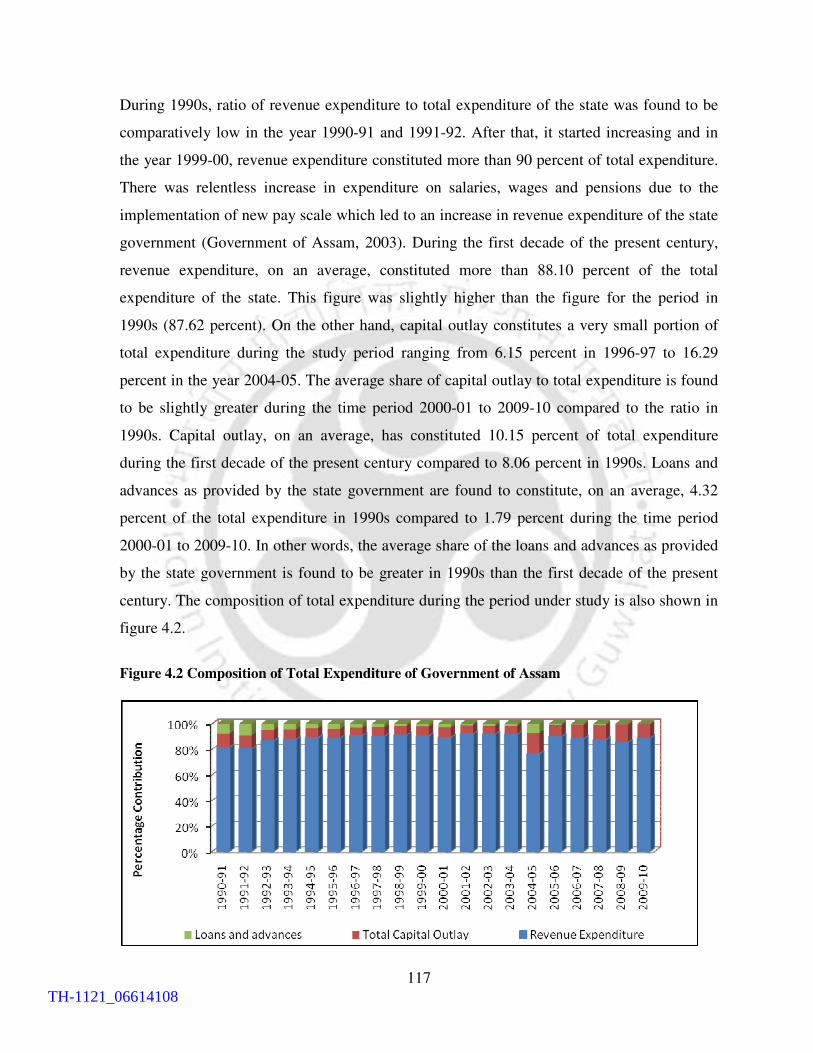
117

During 1990s, ratio of revenue expenditure to total expenditure of the state was found to be

comparatively low in the year 1990-91 and 1991-92. After that, it started increasing and in

the year 1999-00, revenue expenditure constituted more than 90 percent of total expenditure.

There was relentless increase in expenditure on salaries, wages and pensions due to the

implementation of new pay scale which led to an increase in revenue expenditure of the state

government (Government of Assam, 2003). During the first decade of the present century,

revenue expenditure, on an average, constituted more than 88.10 percent of the total

expenditure of the state. This figure was slightly higher than the figure for the period in

1990s (87.62 percent). On the other hand, capital outlay constitutes a very small portion of

total expenditure during the study period ranging from 6.15 percent in 1996-97 to 16.29

percent in the year 2004-05. The average share of capital outlay to total expenditure is found

to be slightly greater during the time period 2000-01 to 2009-10 compared to the ratio in

1990s. Capital outlay, on an average, has constituted 10.15 percent of total expenditure

during the first decade of the present century compared to 8.06 percent in 1990s. Loans and

advances as provided by the state government are found to constitute, on an average, 4.32

percent of the total expenditure in 1990s compared to 1.79 percent during the time period

2000-01 to 2009-10. In other words, the average share of the loans and advances as provided

by the state government is found to be greater in 1990s than the first decade of the present

century. The composition of total expenditure during the period under study is also shown in

figure 4.2.

Figure 4.2 Composition of Total Expenditure of Government of Assam

TH-1121_06614108

118

It can be seen from figure 4.2 that revenue expenditure constitutes a major portion of the total

expenditure during the period of study with periodic changes in the ratio. Decline in the ratio

was observed in the year 2004-05 when revenue expenditure constituted 76.43 percent of

total expenditure. Decline in the share of revenue expenditure in that year was due to increase

in the share of capital expenditure and loans and advances as seen in figure 4.2. Improvement

in the share of capital outlay in the year 2004-05 can be explained by the fact that the state

experienced sharp increase in capital expenditure under economic services. The sharp

increase in capital expenditure under economic services during 2004-05 was mainly due to

investment of ` 1350 crore in public sector undertakings in the energy sector (Government of

Assam, 2005).

To have a clearer idea about the changing composition of total expenditure, it is necessary to

compute growth rate of these variables over the time period. The annual growth of each

components of total expenditure of the state government has been computed for the study

period. Additionally, decade wise compound growth rate has also been computed to have an

idea about the comparative performance of the state in the two decades. The annual and

compound growth rate of these variables has been provided in table 4.3.

TH-1121_06614108

119

Table 4.3

Annual and Compound Growth rate of Components of Total Expenditure of the State

(in percentage)

Year Revenue Expenditure Total Capital

Outlay Loan and Advances Total Expenditure

1 2 3 4 5

1991-92 11.86 15.48 34.05 13.96

1992-93 14.10 -16.82 -42.98 5.59

1993-94 18.37 5.72 9.89 16.89

1994-95 12.74 10.52 -14.56 11.30

1995-96 9.33 8.49 22.01 9.72

1996-97 -0.12 -19.46 -22.32 -2.44

1997-98 13.08 35.97 -12.27 13.69

1998-99 9.35 10.47 -30.36 8.47

1999-00 32.36 32.62 75.26 33.05

2000-01 9.78 16.38 63.05 11.37

2001-02 6.69 -8.61 -62.11 3.42

2002-03 3.89 -1.48 59.38 4.13

2003-04 18.80 23.04 -2.61 18.72

2004-05 21.06 250.57 663.53 45.49

2005-06 3.00 -50.23 -89.16 -12.38

2006-07 8.73 33.88 -23.66 10.77

2007-08 11.24 16.17 77.22 12.20

2008-09 11.76 40.58 -37.71 14.61

2009-10 49.77 10.79 11.24 44.03 CAGR

1990-91 to 1999-00 13.17 7.72 -3.46 11.89

CAGR

2000-01 to 2009-10 14.28 18.71 -8.35 14.30

CAGR

1990-91 to 2009-10 13.51 13.26 -3.17 13.00

Source: Report of the Comptroller and Auditor General of India, Government of Assam, various

issues

Handbook of Statistics of State Government Finances, Reserve Bank of India, various

issues

From table 4.3, the growth rate of revenue expenditure of the state is found to be positive or

moderately negative for most of the year during the period of study. But revenue expenditure

has experienced very high annual growth rate in the year 1999-00 and 2009-10 amounting to

32.36 percent and 49.77 percent respectively. As discussed above, the state government

revised the salary of its employees in the above mentioned year in line with the

TH-1121_06614108

120

recommendations of the Fifth and Sixth Pay Commission of India. It implies that increase in

salary and wages of state government employees has played a significant role in increasing

the revenue expenditure of the state government during the study period. In the year 2004-05,

the capital outlay and loans and advances as provided by the state government registered the

highest ever growth rate amounting to 250.57 percent and 663.53 percent respectively. As

discussed above, the sharp increase in capital outlay in the year 2004-05 was mainly due to

investment of ` 1350 crore in the energy sector. The high increase in loans and advances of

the state government in 2004-05 can be assessed from the fact that state assembly election

was held in 2005-06 which might lead to increase in government expenditure on loans and

advances. Available literature on this issue points out that growth rate of government

expenditure increases during the time of election (Srivastava, 2003; Srivastava, 2009). After

the year 2004-05, the growth rate of these two components of total expenditure was found to

decline in the subsequent years. The compound growth rate of revenue expenditure in the

first decade of the present century is found to be comparatively lower than the previous

decade. The positive development for the state is that it experienced a compound growth rate

of capital expenditure of 18.71 percent during 2000-01 to 2009-10 compared to 7.72 percent

during 1990s. The comparatively high annual compound growth rate of capital expenditure

in the first decade of the present century is mainly contributed by the high growth rate of this

component of expenditure in the year 2004-05. The high growth of capital expenditure may

increase the developmental effectiveness of state government. But compound growth rate of

the loans and advances provided by the state government is found to be negative for both the

time period considered for discussion. This may be due to change in government policy

whereby they stopped providing fresh loans to co-operative societies, corporations and

different companies etc. The trend in the growth rate of different components of total

expenditure is also shown in figure 4.3.

TH-1121_06614108

121

Figure 4.3 Annual Growth Rate of the Components of Total Expenditure

It is evident from figure 4.3 that the growth of revenue expenditure is comparatively uniform

except in the year 1999-00 and 2009-10. But growth rate of capital outlay and state

government’s lending is found to be erratic with sudden surges in some year such as 1999-00

and 2004-05 etc. It is necessary to unearth the reasons for such variations in the growth rate.

A detailed analysis of the sub-components of these broad categories of expenditure gives a

better idea of such variation in the growth rate.

4.3.1 Pattern of Revenue Expenditure:

Generally speaking, revenue expenditure is an amount that is expensed immediately—

thereby being matched with revenues of the current accounting period. Revenue expenditure

is incurred to maintain the current level of services and does not represent any addition to the

state’s service network. The importance of the revenue expenditure lies in the fact that it

helps to maintain and continue the existing level of services. For this, there should be proper

allocation of expenditure on general services, social and community services, economic

services and grants-in-aid (GIA) and contribution etc. The composition of revenue

expenditure of the state of Assam for the period under consideration has been provided in

table 4.4.

TH-1121_06614108

122

Table 4.4

Composition of Revenue Expenditure of Government of Assam (` ` ` ` in lakhs)

Year General Services

Social and Community

Services

Economic

Services

GIA and

Contributions Total

1 2 3 4 5 6

1990-91 59583 (31.03) 78185 (40.71) 53480 (27.85) 792 (0.41) 192040

1991-92 53498 (24.90) 95111 (44.28) 65350( 30.42) 850 (0.40) 214810

1992-93 86564 (35.32) 98525 (40.20) 59364 (24.22) 639 (0.26) 245093

1993-94 103705 (35.75) 121563 (41.90) 63901 (22.03) 948 (0.33) 290117

1994-95 121321(37.09) 131203 (40.11) 73963 (22.61) 584 (0.18) 327071

1995-96 122135 (34.16) 145674 (40.74) 88811 (24.84) 956 (0.27) 357576

1996-97 131639 (36.86) 155334 (43.49) 69751 (19.53) 407 (0.11) 357131

1997-98 155820 (35.58) 174527 (43.22) 73508 (18.20) - 403855

1998-99 159355 (36.58) 196208 (44.43) 85060 (19.26) 1010 (0.23) 441634

1999-00 246190 (42.11) 237755 (40.67) 99959 (17.10) 663 (0.11) 584567

2000-01 254785 (39.70) 281460 (43.86) 104583(16.30) 883 (0.14) 641711

2001-02 292552 (42.73) 270162 (39.46) 121522(17.75) 388 (0.06) 684624

2002-03 311219 (43.76) 289801 (40.75) 109475(15.39) 754 (0.11) 711250

2003-04 352912 (41.77) 336149 (39.78) 154683 (18.31) 1235 (0.15) 844979

2004-05 368891 (36.06) 426242 (41.67) 226470 (22.14) 1311 (0.13) 1022914

2005-06 420161 (39.88) 398710 (37.84) 233671 (22.18) 1089 (0.10) 1053631

2006-07 430236 (37.55) 447748 (39.08) 266889 (23.30) 780 (0.07) 1145653

2007-08 492442 (38.64) 495675 (38.89) 285405 (22.39 894 (0.07) 1274416

2008-09 536133 (37.64) 558225 (38.19) 269330 (18.91) 60613 (4.26) 1424331

2009-10 835688 (39.35) 789128 (37.16) 341418 (16.08) 156988 (7.39) 2123200

CAGR(1990-91 to 1999-00) 17.07 13.15 7.20 -1.96 13.17

CAGR (2000-01 to2009-10) 14.11 12.14 14.05 77.82 14.22

CAGR (1990-91 to 2009-10) 14.91 12.94 10.25 32.10 13.48

Figures in parentheses represent percentage of these variables to total

Source: Directorate of Economics and Statistics, Government of Assam, various issues

It is evident from table 4.4 that major portion of the revenue expenditure of the state has been

incurred on general and social and community services during the time period 1990-91 to

2009-10. During the period of study, revenue expenditure on general services is found to be

comparatively higher than the expenditure on social and community services and economic

services. The compound annual growth rate of general services was found to be 14.91

percent during the time period 1990-91 to 2009-10. For the same time period, expenditure on

TH-1121_06614108

123

social and community services and economic services registered a compound growth rate of

12.94 percent and 10.25 percent respectively implying that growth rate of these components

of expenditure is not compatible with growth rate of general services. Grants-in-aid provided

by the state government constituted less than 1 percent of the total revenue expenditure

during 1990s and registered a compound growth rate of (-) 1.96 percent during that period.

Significant increase in revenue expenditure on grants-in-aid was noticed during the first

decade of the present century which registered a compound growth rate of 77.82 percent. But

increased allocation for grants-in-aid was found to be mainly contributed by the high growth

rate of this component of expenditure in the year 2009-10 amounting to 346.21 percent.

4.3.1.1 Pattern of Revenue Expenditure, General Services:

As expenditure on general services has constituted a major portion of the revenue

expenditure, it is necessary to analyse the composition of revenue expenditure on general

services. The composition of revenue expenditure on general services during the study period

has been provided in table 4.5.

TH-1121_06614108

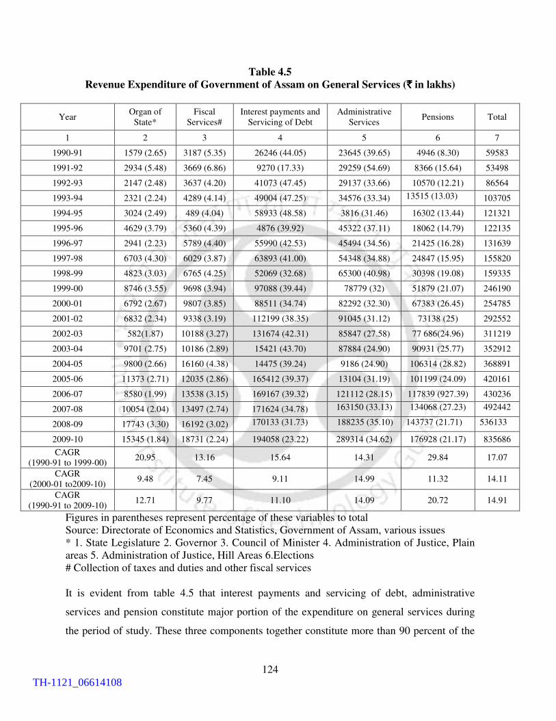
124

Table 4.5

Revenue Expenditure of Government of Assam on General Services (`̀̀̀ in lakhs)

Year Organ of

State*

Fiscal

Services#

Interest payments and

Servicing of Debt

Administrative

Services Pensions Total

1 2 3 4 5 6 7

1990-91 1579 (2.65) 3187 (5.35) 26246 (44.05) 23645 (39.65) 4946 (8.30) 59583

1991-92 2934 (5.48) 3669 (6.86) 9270 (17.33) 29259 (54.69) 8366 (15.64) 53498

1992-93 2147 (2.48) 3637 (4.20) 41073 (47.45) 29137 (33.66) 10570 (12.21) 86564

1993-94 2321 (2.24) 4289 (4.14) 49004 (47.25) 34576 (33.34) 13515 (13.03)

103705

1994-95 3024 (2.49) 489 (4.04) 58933 (48.58) 3816 (31.46) 16302 (13.44) 121321

1995-96 4629 (3.79) 5360 (4.39) 4876 (39.92) 45322 (37.11) 18062 (14.79) 122135

1996-97 2941 (2.23) 5789 (4.40) 55990 (42.53) 45494 (34.56) 21425 (16.28) 131639

1997-98 6703 (4.30) 6029 (3.87) 63893 (41.00) 54348 (34.88) 24847 (15.95) 155820

1998-99 4823 (3.03) 6765 (4.25) 52069 (32.68) 65300 (40.98) 30398 (19.08) 159335

1999-00 8746 (3.55) 9698 (3.94) 97088 (39.44) 78779 (32) 51879 (21.07) 246190

2000-01 6792 (2.67) 9807 (3.85) 88511 (34.74) 82292 (32.30) 67383 (26.45) 254785

2001-02 6832 (2.34) 9338 (3.19) 112199 (38.35) 91045 (31.12) 73138 (25) 292552

2002-03 582(1.87) 10188 (3.27) 131674 (42.31) 85847 (27.58) 77 686(24.96) 311219

2003-04 9701 (2.75) 10186 (2.89) 15421 (43.70) 87884 (24.90) 90931 (25.77) 352912

2004-05 9800 (2.66) 16160 (4.38) 14475 (39.24) 9186 (24.90) 106314 (28.82) 368891

2005-06 11373 (2.71) 12035 (2.86) 165412 (39.37) 13104 (31.19) 101199 (24.09) 420161

2006-07 8580 (1.99) 13538 (3.15) 169167 (39.32) 121112 (28.15) 117839 (927.39) 430236

2007-08 10054 (2.04) 13497 (2.74) 171624 (34.78) 163150 (33.13)

134068 (27.23)

492442

2008-09 17743 (3.30) 16192 (3.02) 170133 (31.73)

188235 (35.10)

143737 (21.71)

536133

2009-10 15345 (1.84) 18731 (2.24) 194058 (23.22) 289314 (34.62) 176928 (21.17) 835686

CAGR

(1990-91 to 1999-00) 20.95 13.16 15.64 14.31 29.84 17.07

CAGR

(2000-01 to2009-10) 9.48 7.45 9.11 14.99 11.32 14.11

CAGR

(1990-91 to 2009-10) 12.71 9.77 11.10 14.09 20.72 14.91

Figures in parentheses represent percentage of these variables to total

Source: Directorate of Economics and Statistics, Government of Assam, various issues

* 1. State Legislature 2. Governor 3. Council of Minister 4. Administration of Justice, Plain

areas 5. Administration of Justice, Hill Areas 6.Elections

# Collection of taxes and duties and other fiscal services

It is evident from table 4.5 that interest payments and servicing of debt, administrative

services and pension constitute major portion of the expenditure on general services during

the period of study. These three components together constitute more than 90 percent of the

TH-1121_06614108

125

revenue expenditure on general services during the study period. The compound growth rate

of expenditure on interest payments, administrative services and pension during the time

period 1990-91 to 2009-10 is found to be 11.10, 14.09 and 20.72 percent respectively. The

growth rate of revenue expenditure on administrative services in the first decade of the

present century was found to be slightly higher than in 1990s. On the other hand, compound

growth rate of revenue expenditure on interest payments and servicing of debt and pensions

was declined during the first decade of the present century compared to the time period 1990-

91 to 1999-00. The initiative by the recent Finance Commissions of India to reduce the

interest burden of the state governments may contribute towards reduction of growth rate of

interest payments of the state during the time period 2000-01 to 2009-10.

4.3.1.2 Pattern of Revenue Expenditure, Social and Community Services:

Apart from the expenditure on general services, it is necessary to analyse the composition of

revenue expenditure on social and community services and economic services which has a

positive impact on the economic development of the state. The composition of expenditure

on social and community services has been provided in table 4.6.

It is evident from table 4.6 that the expenditure on education, sports, art and culture has

constituted the major portion of the revenue expenditure on social and community services

during the time period 1990-91 to 2009-10. On an average, it constitutes almost 64 percent of

the total revenue expenditure on social services during the period of study. But decline in the

share of expenditure on education, sports, art and culture has been noticed during the period

of study. In the year 2009-10, the expenditure on education, sport, art and culture constituted

51.85 percent of the total expenditure on social and community services compared to 57.42

percent in the year 1990-91. The expenditure on medical, family plan, public health and

sanitation constitutes, on an average, 21.36 percent of the total revenue expenditure on social

and community services during the study period. The compound growth rate of medical,

family plan, public health and sanitation is found to be slightly lower than the compound

growth rate of expenditure on education, sports, art and culture during the period taken for

the analysis.

TH-1121_06614108

126

Table 4.6

Revenue Expenditure of Government of Assam on Social and Community Services (`̀̀̀ in

lakhs)

Year Education, Sports, Art

and Culture

Medical, Family Plan,

Public Health and

Sanitation

Others* Total

1 2 3 4 5

1990-91 44894 (57.42) 22448 (28.71) 10753 (13.75) 78185

1991-92 55990 (58.87) 25980 (27.32) 13141 (13.82) 95111

1992-93 64623 (65.59) 22559 (22.90) 11343 (11.51) 98525

1993-94 79191 (65.14) 25768 (21.20) 16604 (13.66) 121563

1994-95 87003 (66.31) 28860 (22.00) 15340 (11.69) 131203

1995-96 97438 (66.89) 32712 (22.46) 15524 (10.66) 145674

1996-97 103462 (66.61) 33999 (21.89) 17873 (11.51) 155334

1997-98 116250 (66.61) 3817 (21.87) 20106 (11.52) 174527

1998-99 136198 (69.42) 36906 (18.81) 23103 (11.77) 196208

1999-00 166437 (70) 47714 (20.07) 23604 (9.93) 237755

2000-01 194116 (68.97) 56751 (20.16) 30593 (10.87) 281460

2001-02 187137 (69.27) 52548 (19.45) 30477 (11.28) 270162

2002-03 199706 (68.91) 51964 (17.93) 38131 (13.16) 289801

2003-04 236248 (70.28) 56438 (16.79) 43463 (12.93) 336149

2004-05 250251 (58.71) 82398 (19.33) 93593 (21.96) 426242

2005-06 251560 (63.09) 82123 (20.60) 65027 (16.31) 398710

2006-07 275112 (61.44) 89728 (20.04) 82908 (18.52) 447748

2007-08 304705 (61.47) 96441 (19.46) 94529 (19.07) 495675

2008-09 329138 (58.96) 123624 (22.14) 105495 (18.90) 558257

2009-10 409194 (51.85) 190086 (24.09) 189848 (24.06) 789128

CAGR

(1990-91 to 1999-00) 15.67 8.74 9.13 13.15

CAGR

(2000-01 to 2009-10) 8.64 14.37 22.49 12.14

CAGR

(1990-91 to 2009-10) 12.33 11.90 16.31 12.94

Figures in parentheses represent percentage of these variables to total

Source: Directorate of Economics and Statistics, Government of Assam, various issues

*includes expenditure on urban development, welfare of SC, ST and OBCs, labour

welfare, social security and welfare, nutrition

TH-1121_06614108

127

4.3.1.3 Pattern of Revenue Expenditure, Economic Services:

As the state suffers from lots of bottlenecks particularly in infrastructure sector, it is

necessary that the state should spend sufficiently on economic services to remove those

bottlenecks. The amount of revenue expenditure on different economic services of the state

has been provided in table 4.7.

It is evident from figure 4.7 that agriculture and allied activities has constituted the major

portion of the revenue expenditure on economic activities during the period of study.

Although the share of this sector has declined due to low growth rate compared to the other

components, but still it constitutes 29.75 percent of the revenue expenditure on economic

services in 2009-10. Increase in the share of rural development has been observed during the

period of study. The share of expenditure on rural development has increased from 15.15

percent in the year 1990-91 to 22.64 percent in the year 2009-10. The compound growth rate

of this component of expenditure during the time period 2000-01 to 2009-10 is found to be

25.20 percent compared to 5.29 percent in 1990s. The compound growth rate of energy is

found to be the highest among the all categories of expenditure as it registered a compound

growth rate of 25.83 percent during the period of study. Transport and communication is

found to be another significant component which shares, on an average, 17.30 percent of the

revenue expenditure on economic services during the study period.

TH-1121_06614108

128

Table 4.7

Composition of Revenue Expenditure on Economic Services (`̀̀̀ in crore)

Year Agriculture and

Allied Activities

Rural

Development

Special Area

Programme

Irrigation and

Flood Control Energy

Industry and

Mineral

Transport &

Communication

General Economic

Services

Science, Technology

and Environment

1 2 3 4 5 6 7 8 9 10

1990-91 24337 (45.51) 8101 (15.15) 570 (1.07) 4409 (8.24) 15 (0.03) 4999 (9.35) 8870 (16.59) 2050 (3.83) 129 (0.24)

1991-92 27831 (42.59) 8864 (13.56) 666 (1.02) 5570 (8.52) 35 (0.05) 8187 (12.53) 11826 (18.10) 2196 (3.36) 175 (0.27)

1992-93 23966 (40.37) 8849 (14.91) 535 (0.90) 5286 (8.90) 22 (0.04) 5974 (10.06) 12485 (21.03) 2098 (3.53) 149 (0.25)

1993-94 25362 (39.69) 10963 (17.16) 712 (1.11) 4455 (6.97) 44 (0.07) 6717 (10.51) 11596 (18.15) 3816 (5.97) 236 (0.37)

1994-95 28600 (38.67) 11492 (15.54) 1196 (1.62) 5060 (6.84) 45 (0.06) 9091 (12.29) 13496 (18.25) 4742 (6.41) 241 (0.33)

1995-96 45782 (51.55) 9855 (11.10) 1417 (1.60) 5069 (5.71) 48 (0.05) 8341 (9.39) 12927 (14.56) 5070 (5.71) 302(0.34)

1996-97 29408 (42.16) 10491 (15.04) 536(0.77) 6025(8.64) 12 (0.02) 5891 (8.45) 13029 (18.68) 4234 (6.07) 125 (0.18)

1997-98 30775 (41.87) 9181 (12.49) 1163 (1.58) 6792 (9.24) 52 (0.07) 6962 (9.47) 13398 (18.23) 5132 (6.98) 53 (0.07)

1998-99 32937 (38.72) 10173 (11.96) 1831 (2.15) 9099 (10.70) 5 (0.01) 9011 (10.59) 16518 (19.42) 5407 (6.36) 80 (0.09)

1999-00 40751 (40.77) 12878 (12.88) 919 (0.92) 10716 (10.72) 14(0.01) 9088 (9.09) 19237 (19.24) 6258 (6.26) 98 (0.10)

2000-01 40622 (38.84) 10178 (9.73) 1302 (1.24) 14718 (14.07) 12 (0.01) 9424 (9.01) 20818 (19.91) 7398 (7.07) 111 (0.11)

2001-02 42542 (35.01) 27424 (22.57) 1872 (1.54) 12628 (10.39) 1816 (1.49) 8040 (6.62) 20451 (16.83) 6593 (5.43) 156 (0.13)

2002-03 36221 (33.09) 21896 (20) 941 (0.86) 12878 (11.76) 508 (0.46) 8716 (7.96) 22238 (20.31) 5980 (5.46) 97 (0.09)

2003-04 47814 (30.91) 26462 (17.11) 2124 (1.37) 17718 (11.45) 14202 (9.18) 9647 (6.24) 24691 (15.96) 11886 (7.68) 139 (0.09)

2004-05 48791 (21.54) 43616 (19.26) 1998 (0.88) 20784 (9.18) 31225(13.79) 12956 (5.72) 30900 (13.64) 35876 (15.84) 324 (0.14)

2005-06 54779 (23.44) 37683 (16.13) 2177 (0.93) 21866 (9.36) 32259(13.81) 13390 (5.73) 34662 (14.83) 36683 (15.70) 172 (0.07)

2006-07 61358 (22.99) 56136 (21.03) 2701 (1.01) 26922 (10.09) 29094 (10.90 11274 (4.22) 38665 (14.49) 40537 (15.19) 201

2007-08 67232 (23.56) 78576 (27.53) 5322 (1.86) 29205 (10.23) 3082 (1.08) 17792 (6.23) 50372 (17.65) 33255 (11.65) 568

2008-09 80349 (29.83) 6515 (24.19) 10596(3.93) 29483(10.95) 8 (.0030) 16908 (6.28) 40339 (14.98) 24601 (9.13) 1894 (0.70)

2009-10 10107 (29.75) 7693 (22.64) 2111 (6.22) 3206 (9.44) 1181 (0.35) 21771(6.41) 51557(15.17) 183(0.05) 33883(9.97)

CAGR (1990-91 to 1999-00) 5.89 5.29 5.45 10.37 -0.76 6.87 8.98 13.20 -3.01

CAGR (2000-01 to2009-10) 10.66 25.20 36.29 9.04 66.51 9.75 10.60 -33.70 88.83

CAGR (1990-91 to 2009-10) 7.78 12.58 20.94 11.01 25.83 8.05 9.71 -11.94 34.07

Source: Figures in parentheses represent percentage of these variables to total

Directorate of Economics and Statistics, Government of Assam, various issues

Handbook of Statistics of State Government Finances, Reserve Bank of India, various issues

TH-1121_06614108

129

4.3.2 Pattern of Capital Expenditure:

Capital expenditure is the amount spent to acquire or improve long-term asset such as

equipment or buildings. For a proper analysis of capital expenditure, it is necessary to

differentiate between capital expenditure and capital outlay. Capital outlay is that part of the

capital expenditure which is used for different activities of the state government which are of

capital nature (RBI, 2007). As mentioned in the section 4.3, capital outlay excludes

expenditures such as discharge of internal debt and repayment of loans to centre. Actually, it

is capital outlay that leads to creation of long term assets (Sarma, 2004). The higher

proportion of capital outlay to capital expenditure helps in development of social and

economic infrastructure of a state. The amount and percentage of capital outlay to total

capital expenditure of the state government has been provided in table 4.8.

Table 4.8

Amount of Capital Expenditure and Capital Outlay of the State Government (` ` ` ` in crore)

Year Capital

Expenditure

Capital

Outlay

Percentage of capital Outlay to

Capital Expenditure 1 2 3 4

1990-91 769 247 32.12

1991-92 615 285 46.34

1992-93 685 237 34.60

1993-94 719 251 34.91

1994-95 727 277 38.10

1995-96 815 301 36.93

1996-97 695 242 34.82

1997-98 984 329 33.43

1998-99 788 364 46.19

1999-00 1240 483 38.95

2000-01 1214 562 46.29

2001-02 1704 513 30.11

2002-03 1824 506 27.74

2003-04 2146 622 28.98

2004-05 4516 2181 48.29

2005-06 1551 1085 69.95

2006-07 2028 1453 71.65

2007-08 2406 1688 70.16

2008-09 3243 2373 73.17

2009-10 5666 4716 83.23

Source: Directorate of Economics and Statistics, Government of Assam, various issues

TH-1121_06614108

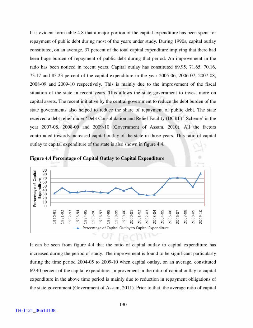
130

It is evident form table 4.8 that a major portion of the capital expenditure has been spent for

repayment of public debt during most of the years under study. During 1990s, capital outlay

constituted, on an average, 37 percent of the total capital expenditure implying that there had

been huge burden of repayment of public debt during that period. An improvement in the

ratio has been noticed in recent years. Capital outlay has constituted 69.95, 71.65, 70.16,

73.17 and 83.23 percent of the capital expenditure in the year 2005-06, 2006-07, 2007-08,

2008-09 and 2009-10 respectively. This is mainly due to the improvement of the fiscal

situation of the state in recent years. This allows the state government to invest more on

capital assets. The recent initiative by the central government to reduce the debt burden of the

state governments also helped to reduce the share of repayment of public debt. The state

received a debt relief under ‘Debt Consolidation and Relief Facility (DCRF) 1

Scheme’ in the

year 2007-08, 2008-09 and 2009-10 (Government of Assam, 2010). All the factors

contributed towards increased capital outlay of the state in those years. This ratio of capital

outlay to capital expenditure of the state is also shown in figure 4.4.

Figure 4.4 Percentage of Capital Outlay to Capital Expenditure

It can be seen from figure 4.4 that the ratio of capital outlay to capital expenditure has

increased during the period of study. The improvement is found to be significant particularly

during the time period 2004-05 to 2009-10 when capital outlay, on an average, constituted

69.40 percent of the capital expenditure. Improvement in the ratio of capital outlay to capital

expenditure in the above time period is mainly due to reduction in repayment obligations of

the state government (Government of Assam, 2011). Prior to that, the average ratio of capital

TH-1121_06614108

131

outlay to capital expenditure of the state was found to be 36.39 percent during the time

period 1990-91 to 2004-05.

4.3.2.1 Composition of Capital Outlay on Different Services:

The composition of capital outlay on different services provides information about the

quality of capital outlay of a state (Das Gupta, 2012). The composition of capital outlay in

terms of general services, social services and economic services has been provided in table

4.9.

Table 4.9

Composition of Capital Outlay of Government of Assam (` ` ` ` in lakh)

Year General services Social Services Economic Services Total Capital Outlay

1 2 3 4 5

1990-91 487 (1.97) 3058 (12.38) 21152 (85.6) 24697

1991-92 666 (2.34) 2509 (8.80) 25346 (88.87) 28521

1992-93 740 (3.12) 2248 (9.48) 20735 (87.40) 23723

1993-94 664 (2.65) 2695 (10.75) 21720 (86.61) 25079

1994-95 986 (3.56) 3330 (12.01) 23402 (84.43) 27718

1995-96 1574 (5.23) 3995 (13.29) 24501 (81.48) 30070

1996-97 484 (2) 1635 (6.75) 22100 (91.25) 24219

1997-98 607 (1.84) 2800 (8.50) 29524 (89.65) 32931

1998-99 340 (0.93) 4643 (12.76) 31397 (86.30) 36380

1999-00 1054 (2.18) 5152 (10.68) 42041 (87.14) 48247

2000-01 787 (1.40) 3469 (6.18) 51892 (92.42) 56148

2001-02 980 (1.91) 3433 (6.69) 46902 (91.0) 51315

2002-03 1125 (2.23) 2195 (4.34) 47233 (93.43) 50553

2003-04 1762 (2.83) 3947 (6.35) 56490 (90.82) 62199

2004-05 2320 (1.06) 4740 (2.17) 210993 (96.76) 218052

2005-06 1041 (0.96) 4507 (4.15) 102984 (94.89) 108532

2006-07 2317 (1.59) 15514 (10.68) 127469 (87.73) 145300

2007-08 4328 (2.56) 26561 (15.73) 137922 (81.70) 168811

2008-09 3564 (1.50) 49438 (20.83) 184299 (77.64) 237301

2009-10 7186 (2.73) 45084 (17.15) 210665 (80.12) 262935

CAGR (1990-91 to 1999-00) 8.96 5.97 7.93 7.72

CAGR (2000-01 to2009-10) 27.86 32.97 16.85 18.71

CAGR (1990-91 to 2009-10) 15.22 15.21 12.86 13.26

Figures in parentheses represent percentage of these variables to total

Source: Directorate of Economics and Statistics, Government of Assam, various issues

TH-1121_06614108

132

From table 4.9, it is evident that expenditure on economic services constitutes the major

portion of total capital outlay during the study period. The compound growth rate of this

component of expenditure is found to be 12.86 percent during the period 1990-91 to 2009-10.

For the same time period, the compound growth rate of general and social services is found

to be 15.22 percent and 15.21 percent respectively implying that the growth rate of these

components of expenditure is comparatively higher than the growth rate of capital

expenditure on economic services. As economic services constitutes major portion of the

capital outlay, it is necessary to analyse the pattern and composition of expenditure on

economic services. The composition and pattern of capital expenditure on economic services

has been provided in table 4.10.

From table 4.10, increase in the capital outlay on economic services has been noticed during

the time period from 2000-01 to 2009-10 compared to the previous decade. The state

registered a compound growth of 16.85 percent on capital expenditure on economic services

during the time period 2000-01 to 2009-10 compared to 7.93 percent in the previous decade.

Water and power development constitute the major portion of the capital outlay of the state

during the period of study. It contributed, on an average, 42 percent of the total capital

expenditure on economic services during the study period. Expenditure on transport and

communication constituted, on an average, 35 percent of the total capital outlay on economic

services for the study period. Capital outlay on industry and minerals is found to be

comparatively low for the entire time period taken for the study. Although it registered a high

growth rate in the first decade of the present century compared to the previous decade, it

shared only 4.81 percent of the capital expenditure on economic services during the period of

study. But the share of agriculture and allied activities has been increasing during the period

under consideration indicating that greater importance is assigned to this sector.

TH-1121_06614108

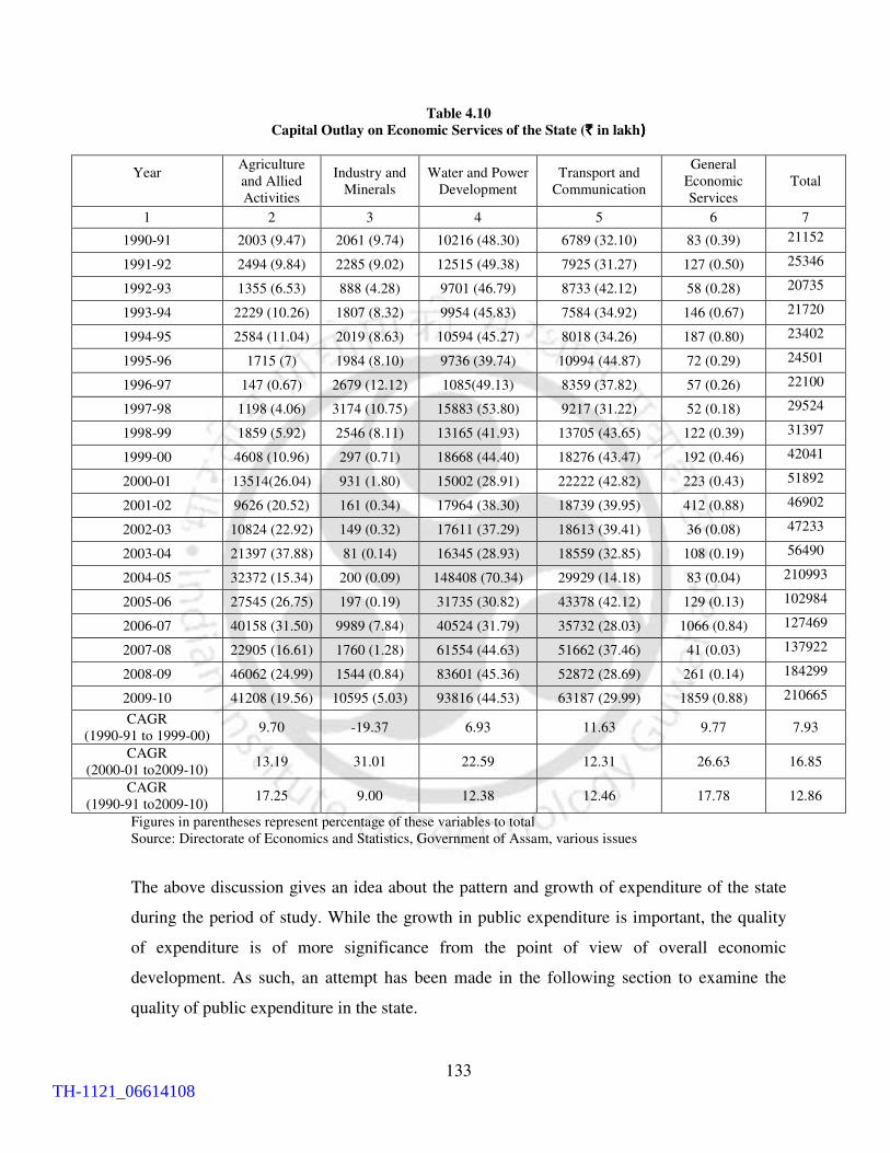
133

Table 4.10

Capital Outlay on Economic Services of the State (` ` ` ` in lakh))))

Year

Agriculture

and Allied

Activities

Industry and

Minerals

Water and Power

Development

Transport and

Communication

General

Economic

Services

Total

1 2 3 4 5 6 7

1990-91 2003 (9.47) 2061 (9.74) 10216 (48.30) 6789 (32.10) 83 (0.39) 21152

1991-92 2494 (9.84) 2285 (9.02) 12515 (49.38) 7925 (31.27) 127 (0.50) 25346

1992-93 1355 (6.53) 888 (4.28) 9701 (46.79) 8733 (42.12) 58 (0.28) 20735

1993-94 2229 (10.26) 1807 (8.32) 9954 (45.83) 7584 (34.92) 146 (0.67) 21720

1994-95 2584 (11.04) 2019 (8.63) 10594 (45.27) 8018 (34.26) 187 (0.80) 23402

1995-96 1715 (7) 1984 (8.10) 9736 (39.74) 10994 (44.87) 72 (0.29) 24501

1996-97 147 (0.67) 2679 (12.12) 1085(49.13) 8359 (37.82) 57 (0.26) 22100

1997-98 1198 (4.06) 3174 (10.75) 15883 (53.80) 9217 (31.22) 52 (0.18) 29524

1998-99 1859 (5.92) 2546 (8.11) 13165 (41.93) 13705 (43.65) 122 (0.39) 31397

1999-00 4608 (10.96) 297 (0.71) 18668 (44.40) 18276 (43.47) 192 (0.46) 42041

2000-01 13514(26.04) 931 (1.80) 15002 (28.91) 22222 (42.82) 223 (0.43) 51892

2001-02 9626 (20.52) 161 (0.34) 17964 (38.30) 18739 (39.95) 412 (0.88) 46902

2002-03 10824 (22.92) 149 (0.32) 17611 (37.29) 18613 (39.41) 36 (0.08) 47233

2003-04 21397 (37.88) 81 (0.14) 16345 (28.93) 18559 (32.85) 108 (0.19) 56490

2004-05 32372 (15.34) 200 (0.09) 148408 (70.34) 29929 (14.18) 83 (0.04) 210993

2005-06 27545 (26.75) 197 (0.19) 31735 (30.82) 43378 (42.12) 129 (0.13) 102984

2006-07 40158 (31.50) 9989 (7.84) 40524 (31.79) 35732 (28.03) 1066 (0.84) 127469

2007-08 22905 (16.61) 1760 (1.28) 61554 (44.63) 51662 (37.46) 41 (0.03) 137922

2008-09 46062 (24.99) 1544 (0.84) 83601 (45.36) 52872 (28.69) 261 (0.14) 184299

2009-10 41208 (19.56) 10595 (5.03) 93816 (44.53) 63187 (29.99) 1859 (0.88) 210665

CAGR

(1990-91 to 1999-00) 9.70 -19.37 6.93 11.63 9.77 7.93

CAGR

(2000-01 to2009-10) 13.19 31.01 22.59 12.31 26.63 16.85

CAGR

(1990-91 to2009-10) 17.25 9.00 12.38 12.46 17.78 12.86

Figures in parentheses represent percentage of these variables to total

Source: Directorate of Economics and Statistics, Government of Assam, various issues

The above discussion gives an idea about the pattern and growth of expenditure of the state

during the period of study. While the growth in public expenditure is important, the quality

of expenditure is of more significance from the point of view of overall economic

development. As such, an attempt has been made in the following section to examine the

quality of public expenditure in the state.

TH-1121_06614108

134

4.4 Quality of expenditure of the State:

Quality of expenditure is basically related to proper allocation of expenditure on different

heads. The availability of resources for improvement in social and physical infrastructure of

the state generally reflects the quality of expenditure (Howes and Jha, 2004; Sen and

Karmakar, 2007). The improvement in the quality of expenditure basically involves two

aspects, viz., adequacy of expenditure (adequate provision for providing public services) and

efficiency of expenditure use. Getting the right size and right composition of government

expenditure to achieve the highest attainable growth rates after meeting the government’s

obligations is known as the adequacy of expenditure. The efficiency of public expenditure

relates to both size and sectoral allocations aimed at removing inefficiencies arising from

misallocations, and implementation of the schemes and delivery of services. In view of the

importance of these factors, the Thirteen Finance Commission gave importance on the need

to improve the quality of public expenditure to obtain better outputs and outcomes (TFC,

2009). It is necessary to determine whether the public expenditure of the state government is

adequate enough to meet the social and economic responsibilities of the government.

4.4.1 Adequacy of Public Expenditure:

The amount of fund available for social and economic services after meeting the expenditure

on general services actually implies the adequacy of expenditure of a state, which is

popularly known as developmental expenditure (Gupta and Sarkar, 1994; Das Gupta, 2012).

The quality of expenditure in terms of adequacy can be assessed by the total developmental

revenue and capital expenditure of the state government during the period of study. The

development expenditure as a ratio of to total and aggregate expenditure as well as GSDP of

the state has been computed to examine the relative growth of development expenditure with

respect to the above mentioned variables. Apart from the components of total expenditure,

aggregate expenditure includes expenditure on repayment of public debt. The amount and

growth of developmental revenue and capital expenditure as well as development

expenditure (DE) of the state has been provided in 4.11.

TH-1121_06614108

135

Table 4.11 Amount and Growth of Developmental Expenditure of the State (`̀̀̀ in crore)

Year Total Developmental

Revenue Expenditure

Total

Developmental

Capital

Expenditure

Developmental

Expenditure(DE)

DE as

percentage of

Total

expenditure

DE as a

percentage of

Aggregate

Expenditure

DE as a

percentage

of GSDP

1 2 3 4 5 6 7

1990-91 1317

(84.47)

242

(15.53) 1559 66.33 57.97 14.68

1991-92 160

(85.21)

279

(14.79) 1883 70.31 68.16 15.89

1992-93 1579

(87.29)

230

(12.71) 1809 63.96 57.68 13.86

1993-94 1855

(88.37)

244

(11.63) 2099 63.50 57.98 13.86

1994-95 2052

(88.47)

267

(11.53) 2319 63.03 58.00 13.21

1995-96 2345

(89.16)

285

(10.84) 2630 65.15 59.90 13.55

1996-97 2251

(90.46)

237

(9.54) 2488 63.19 58.31 11.84

1997-98 2480

(88.47)

323

(11.53) 2804 62.62 55.83 12.29

1998-99 2813

(88.64)

360

(11.36) 3173 65.34 60.97 12.41

1999-00 3377

(87.74)

472

(12.26) 3849 59.57 54.32 11.05

2000-01 3860

(87.46)

554

(12.54) 4414 61.34 57.84 11.99

2001-02 3917

(88.61)

503

(11.39) 4420 59.40 51.70 11.54

2002-03 3993

(88.98)

494

(11.02) 4487 57.90 50.21 10.34

2003-04 4908

(89.04

604

(10.96) 5513 59.92 52.03 11.65

2004-05 6527

(75.16)

2157

(24.84) 8684 64.89 58.90 16.26

2005-06 6324

(85.47)

1075

(14.53) 7399 63.09 61.21 12.46

2006-07 7146

(83.33)

1430

(16.67) 8576 66.02 63.60 13.26

2007-08 7811

(82.60)

1645

(17.40) 9456 64.88 62.41 13.30

2008-09 8276

(77.98)

2337

(22.02) 10613 63.53 60.70 13.07

2009-10 11305

(81.55)

2557

(18.45) 13862 57.85 55.30 14.99

Figures in parentheses represent percentage of this variable to total developmental expenditure

Source: Handbook of Statistics of State Government Finances, Reserve Bank of India, various issues

TH-1121_06614108

136

It is evident from table 4.11 that developmental revenue expenditure of the state government

has increased from ` 1317 crore in 1990-91 to ` 11305 crore in 2009-10 and thus registering

a compound growth rate of 11.98 percent. The compound growth rate of developmental

capital expenditure of the state during the study period is found to be 13.28 percent as it has

increased from ` 242 crore in 1990-91 to ` 11305 crore in 2009-10. The high growth rate of

developmental capital expenditure compared to developmental revenue expenditure implies

that the state has put more effort on creation of capital asset during the period of study.

Compared to this, the compound growth rate of developmental revenue and capital

expenditure of all states is found to be 12.74 and 15.72 percent respectively during the above

mentioned period (RBI, 2011). Again, the compound growth rate of developmental

expenditure of the state during the period of study is found to be 12.19 percent compared to

all states compound growth rate of 13.31 percent (RBI, 2011). Thus, it implies that growth of

development expenditure of the state is not compatible with that of all states average during

the period of study.

Developmental expenditure constituted a major portion of total expenditure of the state

ranging from 70.31 percent in the year 1991-92 to 57.85 percent in 2009-10. On an average,

the developmental expenditure has constituted 62.99 percent of the total expenditure of the

state during the period of study. Compared to this, average ratio of developmental

expenditure to total expenditure of all states during the period of study is found to be 61.54

percent. But the average ratio development expenditure to total expenditure of the special

category states is found to be greater than the state’s average during the period of study. The

average ratio special category state is found to be 65.68 percent compared to the state’s

average of 62.99 percent during the study period. Sudden decline in the ratio of development

expenditure to total and aggregate expenditure of the state is noticed in the year 2009-10.

This is due to the fact that there was a significant increase in total and aggregate expenditure

in the year 2009-10 amounting to 44.03 and 43.37 percent respectively without

commensurate increase in developmental expenditure. Increase in total expenditure in that

year was mainly contributed by increase in revenue expenditure on general services. The

ratio of developmental expenditure as a ratio of GSDP, total expenditure and aggregate

expenditure of the state has been shown in figure 4.5.

TH-1121_06614108

137

Figure 4.5 Development Expenditure as a percentage of GSDP, Total Expenditure and

Aggregate Expenditure of the State

As evident from figure 4.5, development expenditure has maintained a stable ratio with

GSDP for the time period taken for the analysis. The divergence between the ratio of

development expenditure to total and aggregate expenditure of the state is found to decline

during the period of study.

The growth in the absolute value of development expenditure itself is not enough to explain

the process of development, as population is also on the rise. As such, it is necessary to

analyse the per-capita development expenditure in terms of per-capita expenditure on social

services and per-capita expenditure on economic services. The classification of the

developmental expenditure on per-capita basis actually reflects the quality of expenditure

(Shariff et al. 2002; Choudhury, 2002). Here, real per-capita expenditure is used. For doing

this, as done in the previous chapter, the variables are converted into constant 2004-05 prices

by splicing to make it comparable for the whole time period taken for the analysis. Mid-year

population figures have been taken from CSO and price deflators have been computed from

the ratio of current to constant price GSDP figures. The per-capita expenditure on social,

economic and per-capita developmental expenditure of the state has been provided in table

4.12.

TH-1121_06614108

138

Table 4.12

Per-capita Expenditure on Social Services, Economic Services and Developmental

Services (In `)`)`)`)

Year Per-capita Expenditure on

Social Services

Per-capita Expenditure

on Economic Services

Per-capita Development

Expenditure

1 2 3 4

1990-91 955 877 1833

1991-92 1052 977 2029

1992-93 978 777 1755

1993-94 1095 755 1850

1994-95 1032 747 1778

1995-96 1047 792 1839

1996-97 1025 600 1624

1997-98 1061 616 1677

1998-99 1054 611 1666

1999-00 1135 663 1798

2000-01 1276 701 1977

2001-02 1185 730 1915

2002-03 1176 631 1807

2003-04 1313 816 2129

2004-05 1533 1556 3089

2005-06 1315 1098 2413

2006-07 1432 1219 2651

2007-08 1520 1232 2752

2008-09 1632 1218 2850

2009-10 2100 1388 3488

Source: A Handbook of Statistics of State Government Finances, Reserve Bank of India,

various issues

It is evident from table 4.12 that per-capita developmental expenditure has increased from `

1833 in 1990-91 to ` 3488 in 2009-10 and thus registered a compound growth rate of 4.23

percent during that period. Similarly, per-capita expenditure on economic and social services

has increased from ` 955 and ` 877 in 1990-91 to ` 2100 and ` 1388 in 2009-10

respectively. The compound growth rate of these two components of expenditure is found to

be 4.23 and 2.44 percent respectively during the above mentioned period. During 1990s, per-

capita developmental expenditure has declined from ` 1833 in 1990-91 to ` 1798 in 1999-00

and thus registering negative compound growth rate of (-) 0.21 percent. After that, increase

was observed in per-capita development expenditure during the first decade of the present

TH-1121_06614108

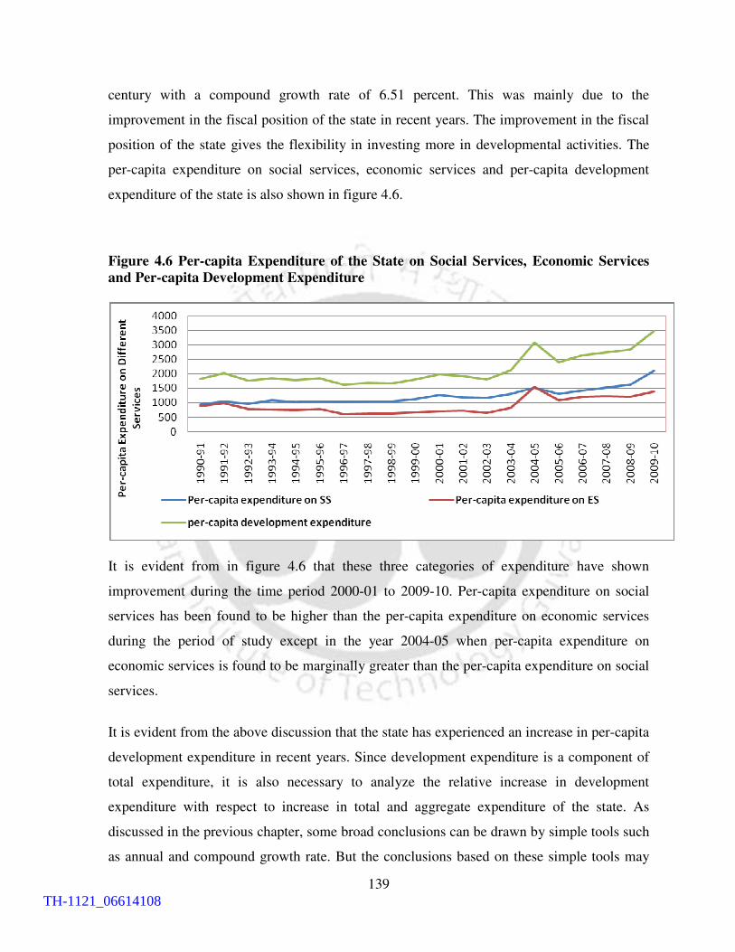
139

century with a compound growth rate of 6.51 percent. This was mainly due to the

improvement in the fiscal position of the state in recent years. The improvement in the fiscal

position of the state gives the flexibility in investing more in developmental activities. The

per-capita expenditure on social services, economic services and per-capita development

expenditure of the state is also shown in figure 4.6.

Figure 4.6 Per-capita Expenditure of the State on Social Services, Economic Services

and Per-capita Development Expenditure

It is evident from in figure 4.6 that these three categories of expenditure have shown

improvement during the time period 2000-01 to 2009-10. Per-capita expenditure on social

services has been found to be higher than the per-capita expenditure on economic services

during the period of study except in the year 2004-05 when per-capita expenditure on

economic services is found to be marginally greater than the per-capita expenditure on social

services.

It is evident from the above discussion that the state has experienced an increase in per-capita

development expenditure in recent years. Since development expenditure is a component of

total expenditure, it is also necessary to analyze the relative increase in development

expenditure with respect to increase in total and aggregate expenditure of the state. As

discussed in the previous chapter, some broad conclusions can be drawn by simple tools such

as annual and compound growth rate. But the conclusions based on these simple tools may

TH-1121_06614108

140

not be rigorous enough and may sometime be misleading too. To be able to draw inferences

in a more rigorous manner, some sophisticated statistical tools should be incorporated.

Keeping this fact in mind, two regression analyses have been carried out to observe the

relative growth of development expenditure with respect to both total and aggregate

expenditure of the state. The time period from 1990-91 to 2009-10 is considered to carry out

this analysis. As the variables are in current prices, they are converted into constant prices by

using appropriate price deflator. The GSDP price deflator is calculated as a ratio of current to

constant prices as done in chapter 3. Gross domestic product data at current and constant

prices in the series 1980-81, 1993-94, 1999-00 and 2004-05 are obtained from the Central

Statistical Organization. All the data are converted into 2004-05 prices by splicing to make it

comparable with the above mentioned series. All the variables are found to be integrated of

order 1. The Dickey Fuller and Philips-Perron unit root test are applied to determine the order

of integration. The regression diagnosis test, called Ljung-Box or Portmanteau test is also

used to test if the residuals of the regression are white noise or it has some autocorrelation

still left. The variables have been transformed in to stationary state before carrying out the

regression analyses. The results of the regression have been provided in table 4.13 and table

4.14.

Table 4.13

Results of the Regression Analysis of Impact of Total Expenditure on Developmental

Expenditure

Variable Coefficient t statistic

Total Expenditure .5899371***

(.0532362)

11.08

Constant -34.53817

(85.13003)

-0.41

R2 0.8009

LB statistic = 7.9126 F( 1, 18) 122.77***

Figures in parentheses represent standard error of the estimated coefficients

***, ** and * indicate significant at 0.01, 0.05 and 0.10 level respectively

TH-1121_06614108

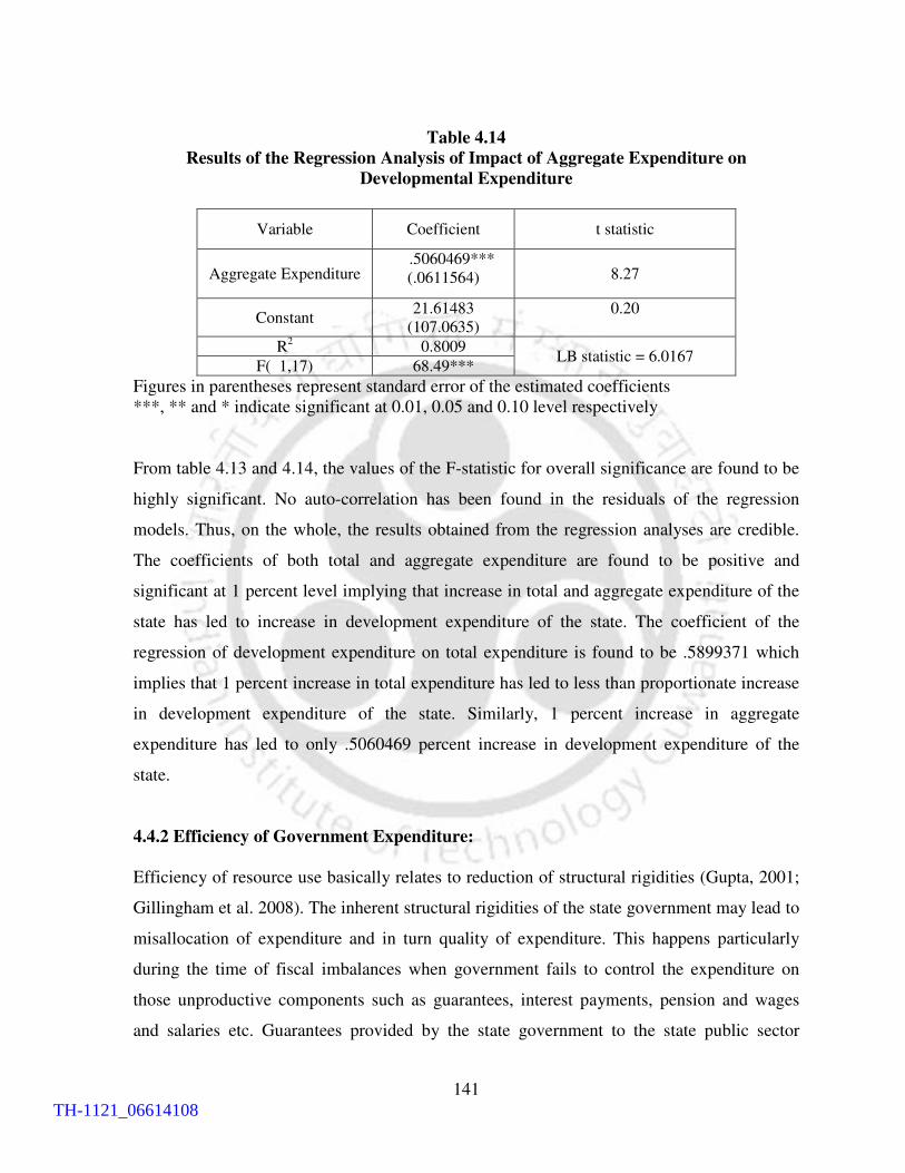
141

Table 4.14

Results of the Regression Analysis of Impact of Aggregate Expenditure on

Developmental Expenditure

Variable Coefficient t statistic

Aggregate Expenditure .5060469***

(.0611564)

8.27

Constant 21.61483

(107.0635)

0.20

R2 0.8009

LB statistic = 6.0167 F( 1,17) 68.49***

Figures in parentheses represent standard error of the estimated coefficients

***, ** and * indicate significant at 0.01, 0.05 and 0.10 level respectively

From table 4.13 and 4.14, the values of the F-statistic for overall significance are found to be

highly significant. No auto-correlation has been found in the residuals of the regression

models. Thus, on the whole, the results obtained from the regression analyses are credible.

The coefficients of both total and aggregate expenditure are found to be positive and

significant at 1 percent level implying that increase in total and aggregate expenditure of the

state has led to increase in development expenditure of the state. The coefficient of the

regression of development expenditure on total expenditure is found to be .5899371 which

implies that 1 percent increase in total expenditure has led to less than proportionate increase

in development expenditure of the state. Similarly, 1 percent increase in aggregate

expenditure has led to only .5060469 percent increase in development expenditure of the

state.

4.4.2 Efficiency of Government Expenditure:

Efficiency of resource use basically relates to reduction of structural rigidities (Gupta, 2001;

Gillingham et al. 2008). The inherent structural rigidities of the state government may lead to

misallocation of expenditure and in turn quality of expenditure. This happens particularly

during the time of fiscal imbalances when government fails to control the expenditure on

those unproductive components such as guarantees, interest payments, pension and wages

and salaries etc. Guarantees provided by the state government to the state public sector

TH-1121_06614108

142

enterprises have been considered as one of the unproductive expenditures of the states in

India (Thorat and Roy, 2004). Guarantees are liabilities contingent on the consolidated fund

of the state in case of default by the borrower from whom the guarantees have been extended.

But when the public sector fails to pay the guarantees, ultimately the state governments have

to repay it. Most of the Public Sector Undertakings in Assam failed to repay the government

guaranteed loans and it became liability of the respective governments. Many enterprises in

Assam work under the psychology that if the state government provides a guarantee, it no

longer is the responsibility of the enterprise to service the debt (Srivastava et al., 1999). To

sort out this problem, the state government laid down the procedure for issues of guarantees

and fixed a ceiling of ` 1,500 crore on guarantees to be given with effect from April 2000

(Government of Assam, 2003). After that, the Government of Assam revised the targets on

guarantees under Assam Fiscal Responsibility and Budget Management Act (AFRBM). As

per AFRBM Act, state government guarantees should be equal to or less than 50 percent of

state’s own tax and non-tax revenues of the second preceding year (Government of Assam,

2010). The outstanding guarantees of the state government during the study period have been

provided in table 4.15.

It is evident from table 4.15 that the outstanding guarantees of the state government increased

from ` 1430 crore in 1998-99 to ` 1883 crore in 2003-04. The Government of Assam failed

to meet the norms on guarantees (a ceiling of ` 1,500 crore) for consecutive years for the

period from 2001-02 to 2003-04. This was a clear case of fiscal indiscipline. The compound

annual growth rate of guarantees provided by the state government was 5.65 percent during

this period. It implied that instead of reducing the amount of guarantees, state government

provided more guarantees to the State Public Sector Enterprises. As most of the Public Sector

Enterprises were not viable, the state government had to repay the guaranteed amount along

with the interest. It ultimately created pressure on revenue expenditure of the state

government. The state was able to meet the revised target on guarantees prescribed by

AFRBM Act for consecutive years during 2004-05 to 2009-10. The outstanding amount of

the guarantees of the state government was found to be below 50 percent of state’s own

revenues of the second preceding year during the above mentioned time period.

TH-1121_06614108

143

Table 4.15

Outstanding Guarantees of the State during the Study Period (`̀̀̀ in crore)

Year Outstanding

Guarantees

As a percentage of State’s Own

Resources of the Second

Preceding year

1 2 3

1991-92 1028 186.91

1992-93 1094 156.73

1993-94 1230 158.71

1994-95 1384 141.51

1995-96 1250 129.94

1996-97 1150 119.92

1997-98 1430 137.76

1998-99 1430 131.31

1999-00 1477 116.94

2000-01 1583 110.31

2001-02 1853 110.96

2002-03 1881 96.96

2003-04 1883 89.71

2004-05 711 27.05

2005-06 1273 42.21

2006-07 904 23.90

2007-08 951 20.27

2008-09 796 14.90

2009-10 299 5.44

Source: Handbook of Statistics of State Government Finances, Reserve Bank of

India, various issues

Report of the Comptroller and Auditor General of India, Government of Assam,

various issues

To have a proper idea about efficiency of public expenditure, it is also necessary to observe

the expenditure on interest payments, pension and salary and wages which are popularly

known as committed expenditure. The higher proportion of committed expenditure to

revenue expenditure reduces the expenditure on maintenance activities which in turn may

deteriorate the existing infrastructure of a state (Jagannathan, 1986). The expenditure on

these three items constitutes a major portion of the revenue expenditure of the state

government. Due to the nature of downward rigidity of these components of expenditure, the

government fails to reduce committed expenditure particularly during the time of fiscal

imbalances. The factors which normally contribute towards enhancement of those

TH-1121_06614108

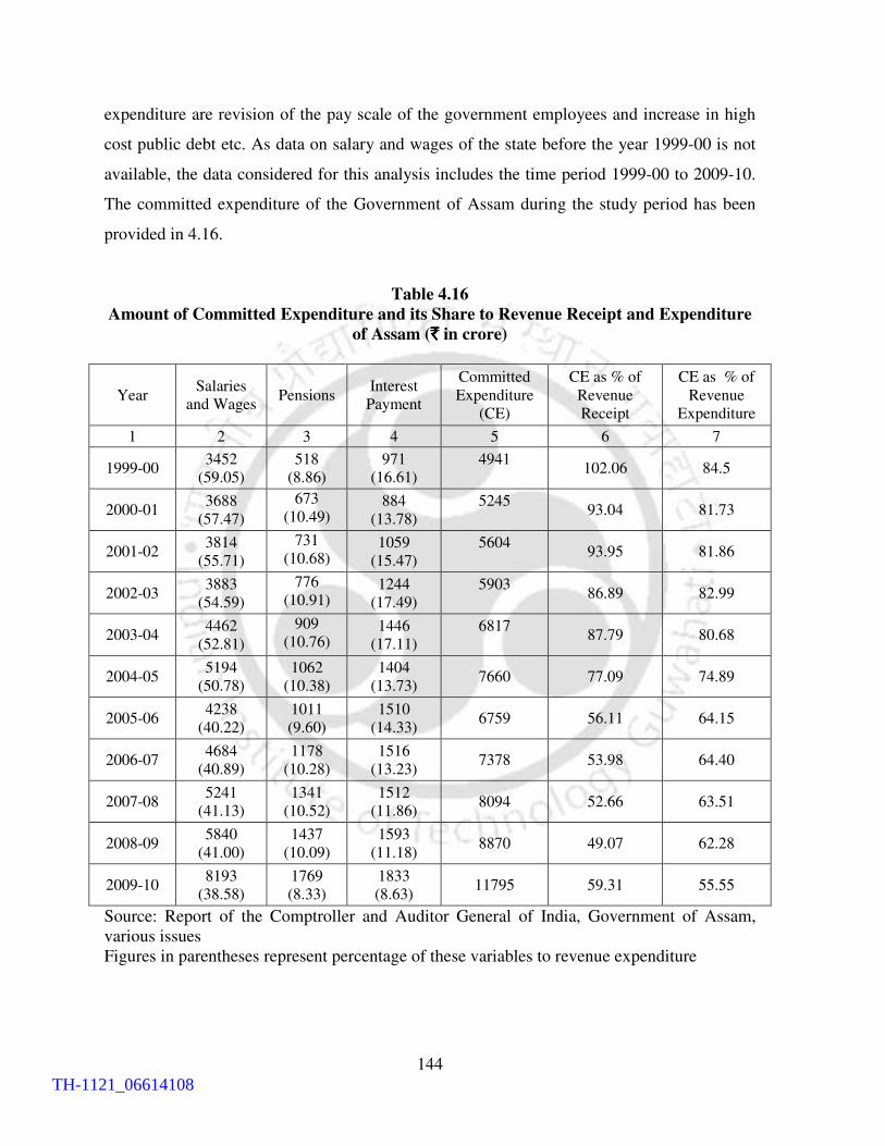
144

expenditure are revision of the pay scale of the government employees and increase in high

cost public debt etc. As data on salary and wages of the state before the year 1999-00 is not

available, the data considered for this analysis includes the time period 1999-00 to 2009-10.

The committed expenditure of the Government of Assam during the study period has been

provided in 4.16.

Table 4.16

Amount of Committed Expenditure and its Share to Revenue Receipt and Expenditure

of Assam (`̀̀̀ in crore)

Year Salaries

and Wages Pensions

Interest

Payment

Committed

Expenditure

(CE)

CE as % of

Revenue

Receipt

CE as % of

Revenue

Expenditure

1 2 3 4 5 6 7

1999-00 3452

(59.05)

518

(8.86)

971

(16.61)

4941

102.06 84.5

2000-01 3688

(57.47)

673

(10.49)

884

(13.78)

5245

93.04 81.73

2001-02 3814

(55.71)

731

(10.68)

1059

(15.47)

5604

93.95 81.86

2002-03 3883

(54.59)

776

(10.91)

1244

(17.49)

5903

86.89 82.99

2003-04 4462

(52.81)

909

(10.76)

1446

(17.11)

6817

87.79 80.68

2004-05 5194

(50.78)

1062

(10.38)

1404

(13.73) 7660 77.09 74.89

2005-06 4238

(40.22)

1011

(9.60)

1510

(14.33) 6759 56.11 64.15

2006-07 4684

(40.89)

1178

(10.28)

1516

(13.23) 7378 53.98 64.40

2007-08 5241

(41.13)

1341

(10.52)

1512

(11.86) 8094 52.66 63.51

2008-09 5840

(41.00)

1437

(10.09)

1593

(11.18) 8870 49.07 62.28

2009-10 8193

(38.58)

1769

(8.33)

1833

(8.63) 11795 59.31 55.55

Source: Report of the Comptroller and Auditor General of India, Government of Assam,

various issues

Figures in parentheses represent percentage of these variables to revenue expenditure

TH-1121_06614108

145

It is evident from table 4.16 that during the period 1999-2004, committed expenditure, on an

average, constituted more than 80 percent of revenue expenditure leaving little fund available

for developmental activities. Similar to this, committed expenditure constituted, on an

average, more than 92 percent of revenue receipt during the same period implying that

revenue earned by the government was used mainly to pay salaries and wages, pension and

interest payments. The percentage share of committed expenditure to revenue receipt was

found to be the highest in the year 1999-00 when it constituted more than 100 percent

(102.06%) of revenue receipt. It implies that even the entire revenue earned by the state was

not sufficient to meet the committed expenditure and borrowed funds were used to meet that

expenditure in that year. But significant improvement was noticed during the time period

2005-06 to 2008-09 as government was able to reduce the ratio in the above mentioned years.

In the year 2008-09, committed expenditure constituted 49.07 percent of the revenue receipt

and 62.28 percent of the revenue expenditure of the state. This reflects better efficiency of

government expenditure as more funds are available for the state after meeting the committed

expenditure. As improvement in quality of expenditure has been observed in recent years, it

is necessary to analyse the reasons for such improvement in expenditure quality of the state.

Actually, the state has undertaken different reform measures in recent years particularly

aimed at reduction of government expenditure. Under these circumstances, it is necessary to

analyse the role of those reform measures in controlling expenditure of the state government.

4.5 Expenditure Implication of Different Fiscal Reform Measures:

As existing review of literature indicates that although revenue enhancement is a desirable

instrument for fiscal adjustment, but fiscal consolidation attempted through reduction of

expenditure are found to be more successful. But in a state like Assam, where state

government has to play a significant role in economic development, cuts in expenditure may

have serious consequences in terms of reduction of expenditure in desired areas. The

continuing fiscal imbalances of the state in the 1990s forced the Assam government to

undertake various expenditure reform measures. A few of them are outlined below:

TH-1121_06614108

146

4.5.1 Agreements with the Central Government:

In pursuance of the decision taken by the Committee of the National Development Council,

an agreement was signed (13 January, 2000) between Ministry of Finance, Government of

India and the State Government regarding measures to be adopted to deal with the fiscal

imbalances arising out of the revenue deficits and resultant recurring overdrafts of the State

Government (Government of Assam, 2001). A Memorandum of Understanding (MoU) was

signed by the State Government with the Central Government on March 26, 2003. The key

performance indicator as detailed in the MoU was to reduce the ratio of revenue deficit to

revenue receipts by five percentage points every year from an estimated 14.54 percent in

2000-01 to 0.84 percent in 2004-05. The state government was not able to achieve this target

as the ratio declined from 13.82 percent in 2000-01 to 2.92 percent in 2004-05 (Government

of Assam, 2003).

4.5.2 Fiscal Responsibility Legislation: A major fiscal development of the state of Assam in

terms of fiscal reforms was the adoption of the Assam Fiscal Responsibility and the Budget

Management Act (AFRBM) in line with the recommendation of the Twelfth Finance

Commission. The act was influenced by Maastricht Treaty and U. K. Golden rule

(Srivastava, 2003). The AFRBM Act was enacted in May 2005 to ensure fiscal stability,

sustainability, improve efficiency and transparency in public finances. The Act prescribed

different fiscal targets for the state government such as elimination of revenue deficit, reduce

the fiscal deficit to 3 percent of GSDP, expenditure on account of salary and wages of the

employees of the State Government to be contained within 60 percent of the total tax and

non-tax revenue of the State Government and restrict the total debt stock of the state

government including the government guarantees to 45 percent of the GSDP etc.

4.5.3 New Pension Scheme: The expenditure on pension is one of the biggest liabilities of

the state government. Pension expenditure has been increasing at a very high rate during

nineties of the previous century as discussed in the above sections. Considering the gravity of

the problem, the Central government urged the state government to impose new pension

scheme. Karnataka was the first state to implement the new pension scheme in September

2002. The Government of Assam introduced the New Pension Scheme in September 2002.

TH-1121_06614108

147

4.5.4. Consolidated Sinking Fund: Another important fiscal development for the state was

that in line with the recommendations of the Twelfth Finance Commission, the state

government set up the Sinking fund for amortization of the market borrowings as well as

other loans and debt obligations. As on 31 March 2009-10, the balance in the sinking fund

was ` 1056.75 crore. During the year 2009-10, ` 108 crore was invested in the sinking fund.

All the above mentioned reform measures have helped the state to achieve the target on

expenditure as particularly set by the Assam Fiscal Responsibility and Budget Management

Act (RBI, 2010; Government of Assam, 2009). As discussed above, significant decline in

percentage of revenue expenditure on salaries and wages, pension and interest payments has

been observed during the time period 2005-06 to 2008-09. Similarly, decline in percentage of

revenue expenditure on guarantees has been observed in the first decade of present century

compared to the previous decade. But reduction of expenditure is not the only objective of

the state government. The reform measures must ensure that there is no lack of fund for

different expenditure responsibilities of the state. Additionally, quality of expenditure should

be comparable to other states of the country. Considering the above fact, a composite

expenditure management index has been computed including some of the important

dimensions of management of expenditure.

4.6 Composite Expenditure Management Index (EMI):

From the above analysis, it is quite clear that expenditure management is a multi-dimensional

concept which cannot be explained with the help of a single indicator. As a single indicator is

unable to explain the quality of expenditure, it is required to construct a composite index

capturing the important components of expenditure. The following parameters have been

selected for construction of the expenditure management index.

1. Ratio of Development Expenditure to Total Expenditure (DE/TE)

2. Ratio of Capital Expenditure to Total Expenditure (CE/TE)

3. Ratio of Revenue Expenditure being met by Own Resources in terms of Own tax and

Non-tax (OW/RE)

4. Ratio of Interest Payments to Revenue Receipt (IP/RR)

TH-1121_06614108

148

As used in the revenue chapter, the methodology applied for construction of this index is

similar to the Human Development Index of UNDP. In all the parameters, no normal or goal

post value has been defined. The observed maximum value of the parameters during the

study period has been taken as the maximum or goal post value. In case of the parameters

where a decline in the value would indicate an improvement, inverse of the observed values

have been used in computing the index. For aggregation of the different dimensions,

geometric mean is used as it gives more weightage to the lower values. The index is

computed for two sub-periods. As, geometric mean is used for aggregation, natural zeros are

used as a minimum value of the parameters. The dimension of each parameter is expressed as

a value between 0 and 1 by applying the following formula.

Actual Value - Minimum ValueDimension Index =

Maximum Value - Minimum Value

From the above dimension index, it is clear that the state whose performance is found to be

the best gets the maximum value of 1. But in case of the interest payments-revenue receipts

ratio, the state whose performance is found to be the worst gets the maximum value of 1. As

natural zeros are used as minimum values, the lowest performer among all the states gets the

minimum value which is greater than 0. The time period taken for the analysis is from 2000-

01 to 2009-10. Although the study period covers the time period 1990-91 to 2009-10, the

dimension index includes only the first decade of the present century. This is due to lack of

data on each of the state during 1990s. The index is computed for two sub-periods with five

year average so that it is not highly influenced by the value of a particular year. The

dimension indices of development expenditure to total expenditure, capital expenditure to

total expenditure, revenue expenditure to own resources and interest payments to revenue

expenditure have been computed separately by applying the above discussed formula. D1, D2,

D3, and D4 are used to represent the value of the dimension index for the parameters

development expenditure to total expenditure, capital expenditure to total expenditure,

revenue expenditure to own resources and interest payments to revenue expenditure

respectively. The computed expenditure management index has been given in table 4.17 and

4.18.

TH-1121_06614108

149

Table 4.17

Expenditure Management Index for the Time Period 2000-05

States DE/TE CE/TE RE/OW IP/RE D1 D2 D3 D4 EMI

1 2 3 4 5 6 7 8 9 10

Assam 0.607 0.241 0.341 6.541 0.839 0.569 0.391 0.406 0.525

Andhra Pradesh 0.655 0.274 0.609 4.898 0.905 0.648 0.699 0.304 0.594

Bihar 0.513 0.224 0.244 4.717 0.709 0.530 0.280 0.293 0.419

Chhattisgarh 0.663 0.217 0.596 6.370 0.916 0.513 0.684 0.396 0.597

Goa 0.617 0.198 0.806 6.060 0.852 0.468 0.924 0.376 0.610

Gujarat 0.650 0.261 0.617 4.911 0.898 0.618 0.707 0.305 0.588

Haryana 0.570 0.234 0.816 4.967 0.787 0.554 0.936 0.309 0.596

Jharkhand 0.658 0.257 0.456 8.512 0.909 0.607 0.523 0.529 0.625

Karnataka 0.614 0.234 0.681 6.389 0.848 0.554 0.781 0.397 0.618

Kerala 0.532 0.155 0.558 4.872 0.735 0.367 0.640 0.303 0.478

Madhya Pradesh 0.622 0.249 0.520 5.911 0.859 0.589 0.596 0.367 0.577

Maharashtra 0.580 0.213 0.677 5.919 0.802 0.503 0.776 0.368 0.583

Orissa 0.507 0.262 0.376 3.665 0.701 0.619 0.431 0.228 0.454

Punjab 0.533 0.260 0.872 3.408 0.737 0.615 1.000 0.212 0.556

Rajasthan 0.591 0.246 0.480 4.073 0.817 0.582 0.551 0.253 0.507

Tamil Nadu 0.564 0.211 0.681 6.165 0.779 0.500 0.781 0.383 0.584

Uttar Pradesh 0.534 0.236 0.394 4.282 0.738 0.559 0.453 0.266 0.472

West Bengal 0.462 0.227 0.346 3.325 0.638 0.538 0.397 0.207 0.410

Arunachal 0.724 0.302 0.114 9.057 1.000 0.714 0.130 0.563 0.478

Manipur 0.618 0.423 0.080 6.391 0.855 1.000 0.091 0.397 0.420

Meghalaya 0.637 0.244 0.207 8.634 0.880 0.576 0.237 0.536 0.504

Mizoram 0.680 0.227 0.067 8.344 0.940 0.537 0.077 0.518 0.377

Nagaland 0.577 0.261 0.075 7.057 0.797 0.616 0.086 0.438 0.369

Sikkim 0.428 0.175 0.627 16.099 0.591 0.414 0.720 1.000 0.648

Tripura 0.617 0.289 0.172 6.965 0.853 0.684 0.197 0.433 0.472

Himachal Pradesh 0.616 0.276 0.241 4.317 0.851 0.654 0.277 0.268 0.451

Jammu and

Kashmir 0.591 0.243 0.205 6.409 0.817 0.576 0.235 0.398 0.458

Uttarakhand 0.664 0.239 0.381 7.038 0.917 0.565 0.437 0.437 0.561

All States 0.572 0.234 0.520 4.952 0.790 0.553 0.638 0.308 0.541

Source: Calculated by the author (basic data from various issues of Handbook of Statistics of

State Government Finances, Reserve Bank of India and CSO reports)

TH-1121_06614108

150

Table 4.18

Expenditure Management Index for the Time Period 2005-10

States DE/TE CE/TE RE/OW IP/RE D1 D2 D3 D4 EMI

1 2 3 4 5 6 7 8 9 10

Assam 0.627 0.163 0.369 9.612 0.761 0.447 0.423 0.562 0.533

Andhra Pradesh 0.701 0.284 0.687 6.862 0.851 0.779 0.789 0.401 0.677

Bihar 0.654 0.258 0.224 6.869 0.794 0.707 0.257 0.402 0.491

Chhattisgarh 0.824 0.288 0.775 9.372 1.000 0.788 0.889 0.548 0.787

Goa 0.701 0.231 0.826 2.936 0.851 0.634 0.948 0.172 0.544

Gujarat 0.665 0.247 0.745 4.642 0.808 0.678 0.855 0.272 0.597

Haryana 0.701 0.190 0.871 7.709 0.851 0.520 1.000 0.451 0.668

Jharkhand 0.665 0.268 0.442 9.871 0.807 0.735 0.507 0.577 0.646

Karnataka 0.680 0.230 0.775 8.181 0.826 0.629 0.889 0.479 0.686

Kerala 0.480 0.132 0.606 5.483 0.583 0.362 0.695 0.321 0.466

Madhya Pradesh 0.634 0.270 0.555 6.492 0.769 0.739 0.637 0.380 0.609

Maharashtra 0.647 0.217 0.794 5.851 0.786 0.595 0.912 0.342 0.618

Orissa 0.589 0.178 0.464 5.311 0.716 0.489 0.533 0.311 0.491

Punjab 0.477 0.192 0.686 5.126 0.579 0.527 0.787 0.300 0.518

Rajasthan 0.657 0.223 0.577 4.966 0.798 0.612 0.663 0.291 0.554

Tamil Nadu 0.585 0.220 0.765 7.902 0.711 0.603 0.878 0.462 0.646

Uttar Pradesh 0.611 0.257 0.471 6.313 0.741 0.703 0.540 0.369 0.568

West Bengal 0.525 0.200 0.380 3.719 0.637 0.549 0.436 0.218 0.427

Arunachal 0.780 0.326 0.189 12.478 0.947 0.893 0.217 0.730 0.605

Manipur 0.665 0.365 0.120 8.489 0.807 1.000 0.138 0.497 0.485

Meghalaya 0.703 0.196 0.218 11.700 0.853 0.537 0.250 0.684 0.529

Mizoram 0.712 0.250 0.109 8.212 0.865 0.685 0.125 0.480 0.434

Nagaland 0.613 0.310 0.098 8.640 0.744 0.848 0.113 0.505 0.436

Sikkim 0.474 0.220 0.618 17.095 0.575 0.603 0.709 1.000 0.704

Tripura 0.603 0.294 0.167 7.927 0.733 0.806 0.192 0.464 0.478

Himachal Pradesh 0.629 0.263 0.398 4.745 0.764 0.720 0.457 0.278 0.514

Jammu and Kashmir 0.658 0.319 0.275 7.585 0.799 0.874 0.315 0.444 0.559

Uttarakhand 0.644 0.255 0.458 6.798 0.782 0.698 0.526 0.398 0.581

All States 0.639 0.216 0.538 7.191 0.776 0.592 0.618 0.421 0.588

Source: Calculated by the author (basic data from various issues of Handbook of Statistics of

State Government Finances, Reserve Bank of India and CSO reports)

TH-1121_06614108

151

From table 4.17 and 4.18, it has been found that the value of expenditure management

indices is low compared to most of the other states in India as well as all states average.

Slight improvement of the value of the indices has been observed in the sub-period 2005-10

compared to the previous sub-period. The value of the indices has increased from 0.525 in

2000-05 to 0.533 in 2005-10. The poor performance of the state was due to the fact that the

ratio of development expenditure to total expenditure, capital expenditure to total expenditure

and own resources to revenue expenditure was low compared to other states. In other words,

the quality of expenditure of Assam is not comparable to other developed states in India.

4.7 Conclusion:

From the above discussion, it is quite clear that there has been significant increase in total

expenditure of the state during the period of study. Wide fluctuations have been observed in

annual growth rate of total expenditure during the study period. The total expenditure-GSDP

ratio of the state is found to increase during the period of study with the increase in GSDP

implying the applicability of Wagner law in the state. The composition of total expenditure

reveals that revenue expenditure has a dominant share in total expenditure of the state leaving

fewer resources available for capital expenditure and for advancement of loans and advances

for developmental purposes. The average ratio of revenue expenditure to total expenditure of

the state is found to be higher than all states average during the period of study. The capital

outlay constitutes, on an average, less than 10 percent of the total expenditure of the state

during the study period. The average ratio of capital outlay to total expenditure of the state is

found to be less compared to all states average during the period of study. Similarly, the

average ratio of loans and advances to the total expenditure of the state is found to be low

compared to the all states average during the period taken for the analysis. The loan and

advances provided by the state government, on an average, comprises less than 1 percent of

the total expenditure for the study period.

Among the constituents of revenue expenditure, expenditure on general services has been

found to accounts for the major portion of revenue expenditure during the period of study.

The administrative services, pension and interest payments constitute the major portion of the

revenue expenditure on general services. The increase in salaries and wages of the employees

TH-1121_06614108

152

due to implementation of Fifth and Sixth Pay Commission’s recommendations in the year

1999-00 and 2009-10 also contributes towards increased expenditure on general services.

The positive fiscal development for the state during the study period is that there has been

increase in the share of capital outlay to total capital expenditure which provides opportunity

for allocation of resources for creation of social and physical assets instead of repayment of

public debt. The composition of capital outlay reveals that expenditure on economic services

constitutes major portion of the expenditure on capital outlay.

Increase in developmental expenditure of the state government during the study period

implies that more resources are available for social and economic services. But decline in the

ratio of development expenditure to total expenditure as well as development expenditure to

aggregate expenditure of the state has been observed during the period of study. The

compound growth rate of developmental expenditure of the state is found to be less than total

and aggregate expenditure of the state. The average ratio of development expenditure to total

expenditure of the state is found to be greater than all states average during the study period.

But the ratio is found to be lower than the average value of the special category states. The

regression results show less than proportionate growth of development expenditure with

respect to both total and aggregate expenditure of the state.

The expenditure on guarantees has been declining significantly as guarantees outstanding

constitute only 5.44 percent of the state’s own resources of the second preceding year in the

year 2009-10. Decline in the ratio of commuted expenditure to revenue receipts and revenue

expenditure has been observed during the time period 2005-06 to 2008-09. The decline is

found to be significant in case of interest payments as payments of interest constitutes only

8.63 percent of the revenue expenditure in the year 2009-10. It is well below the target of the

Twelfth Finance Commission.

Different fiscal reform measures adopted by the state government particularly during the time

period 2005-06 to 2009-10 has helped to control the total expenditure of the state. But recent

increase in total expenditure in the year 2009-10 is matter of concern for the state

government. The computed value of the expenditure management index of the state is found

TH-1121_06614108

153

to be low compared to the other developed states and all states average for both the time

period taken for the analysis. It implies that overall management of expenditure of the state is

comparatively low than other developed states in India. But slight improvement of the

indices has been observed during the time period 2005-06 to 2009-10 compared to 2000-01

to 2004-05. The state government has to put effort for better management of public

expenditure. At the same time, efforts are required to maintain the existing quality of

expenditure through fiscal stability. To ensure fiscal stability, state government has to

maintain a sustainable fiscal policy. An unsustainable fiscal policy may lead to deterioration

of the deficit indicators of the state. Under these circumstances, there is need to have a

detailed analysis of fiscal and debt sustainability of the state.

Note:

1. DCRF: In Pursuance of the recommendations of the Twelve Finance Commission (TFC) for

fiscal consolidation and elimination of revenue deficit of the State, Government of India

formulated this scheme (2005-06 to 2009-10) under which general debt relief is provided by

consolidating and rescheduling at substantially reduced rates of interest, the Central loans

granted to the States on enacting the FRBM Act and debt waiver is granted based on fiscal

performance, linked to reduction in revenue deficits of States.

****

TH-1121_06614108

154

TH-1121_06614108

155

Chapter 5

Fiscal and Debt Sustainability of the State

In the previous chapter, the pattern and composition of government expenditure has been

studied to see the growth and quality of public expenditure of the state. Implication of recent

fiscal reform measures on government expenditure has also been examined to know the

allocation and prioritization of expenditure. Available literature states that proper allocation

of resources with emphasis on developmental expenditure is the main requirement for overall

development of the states (Howes et al, 2004; Dasgupta, 2012). The state needs sufficient

amount of revenues to discharge those expenditure responsibilities. Otherwise, there will be

imbalances between total resources of the government and their expenditure obligations.

Under these circumstances, it is pertinent to study whether total receipts of the state

government are sufficient to meet the expenditure responsibilities of the government.

Available literature on this issue opines that while revenue receipts of the governments

should be adequate to meet the revenue expenditure, capital expenditure could be incurred

out of the borrowed funds (Srivastava, 2009; Rao, 2002; Lahiri, 2000). The above two rules

are basically influenced by the Maastricht Treaty and U.K. Golden rule. The Maastricht

Treaty which was signed in February 1992 by the members of the European community in

Maastricht, Netherlands stated that country’s overall budget deficit for each fiscal year must

be equal to or below 3 percent of GDP. The U.K. has been operating a Golden rule since

1997 whereby borrowing should be made only to finance capital spending. Fiscal imbalances

of a state generally occur mainly due to excessive growth of expenditure and inability of the

state government to meet that expenditure out of their revenue and capital receipts. The

theoretical underpinning of the budget deficit lies in the fact that until the Keynesian

revolution (Keynes, 1936), budget deficits were considered as signs of profligacy.

Governments were often forced to incur large deficits in times of war or natural calamities;

but the prudent ones used to pay off debt by running surplus budget when normalcy had

returned (Rajaraman and Mukhopadhyay, 2005). With the advent of Keynesian economics,

budget deficit was even considered essential for macro stabilization. Counter-cyclical fiscal

policies require the government to run budget deficits in times of demand deficiency and

fiscal squeeze during booms. If the business cycle is symmetrical around the economy’s full

TH-1121_06614108

156

employment growth path, such policies help to keep the budget balance over a typical cycle

and there is no tendency for a secular increase in public debt. But if the budget deficit is

chronic instead of cyclical, then resulting accumulation of debt make the budgetary process

unsustainable. Debt financing is problematic in the demand deficient economy when the

deficiency is chronic or structural rather than cyclical (Rakshit, 2005).

There is a growing awareness among the states in India in recent decades to contain fiscal

imbalances which has led to accumulation of debt and deterioration in the fiscal indicators

(Rao, 2002; Srivastava, 2009). Earlier, most Indian economists were of the view that the

growth of public debt in planned magnitude was normal and desirable in a developing

country like India where borrowing represents the absorption by the government of a part of

domestic savings and the inflow of capital from abroad to finance and promote capital

formation in the public sector and priority areas in the private sector (Chelliah, 1996). But

this view was based on the assumption that borrowed funds would be used only for capital

purposes and the resultant investment would yield adequate direct and or indirect returns. But

these assumptions were not often fulfilled in case of both central and state governments in

India. The fiscal crisis and the resultant exponential growth of public debt in India in later

part of 1990s was not merely because of rising revenue expenditure ahead of current

revenues, but also because capital expenditure financed by borrowings did not yield adequate

returns (Chelliah, 1996). The deterioration in the fiscal indicators and rising public debt of

the state governments in India during that period disrupted the normal functioning of the

economy (Rao, 2005). Deterioration in the fiscal indicators of the state governments

contributed towards macroeconomic instability of the whole nation. Considering that fact, the

recent Finance Commissions of Government of India in their terms of reference have given

importance on fiscal and debt sustainability (TFC, 2009). A sustainable fiscal policy helps a

state to maintain a stable fiscal position without undertaking drastic and painful reforms

measures. The significance of fiscal sustainability is more for poor and backward states as

deterioration in their fiscal position may hamper the overall economic development of those

states. As Assam is a poor state with lots of deficiencies particularly in the infrastructure

sector, it is necessary to study the sustainability of the fiscal position of the state. Considering

TH-1121_06614108

157

the significance of fiscal and debt sustainability on state finances, issue of fiscal and debt

sustainability of the state has been carried out in this chapter.

5.1 Theoretical Framework for Examining Fiscal and Debt Sustainability:

The issue of fiscal sustainability and solvency is usually addressed by analyzing the variables

such as growth rate of GSDP, average interest rate on public debt and growth rate of public

debt etc. The concept of solvency and sustainability are closely related in the sense that an

unsustainable time path will ultimately threaten the solvency of a state (Rajaraman et al.,

2005). The earlier statement of debt dynamics by Domar (1944) remains the simplest guide

for the policy maker for fiscal and debt sustainability which states that “If the government

finances a part of the expenditure (amounting to a given fraction of full employment output)

through borrowings, in a growing economy, public debt and the government interest outgo as

a proportion of GDP will be stable in the long run provided that growth rate exceeds the

interest rate.” Subsequent restatements in terms of infinite horizon constraint on the present

discounted value (PDV) of debt have not changed the fundamental Domar condition for

stabilization of debt as a ratio to GDP (Rajaraman, 2005; Rakshit, 2005; Rath, 2005). Fiscal

and debt sustainability of the state have been analysed with the help of the following

equations as provided below.

According the Domar’s model for solvency of public debt,

t0 t

PDD - .............................(i)

(1+r)= ∑

Here, D0 = Present stock of outstanding debt

PDt = Primary deficit for the time period t

r = interest rate on public debt

The above equation implies that for solvency, present outstanding stock of public debt must

be equal to the summation of discounted primary surplus of future years expressed in terms

of present value. Primary deficit incurred in a particular year can be expressed as,

t t t-1PD D -(1+r)D ....................................(ii)=

TH-1121_06614108

158

Equation (ii) simply states that primary deficit plus interest on past debt (rDt-1) has to be

financed by a built-up debt itself (Dt –Dt-1) (Lahiri and Kannon, 2004).

Now, equation (i) can be rewritten by replacing the value of PDt as obtained from equation

(ii)

t t-10 t

D -(1+r)D D - ............................(iii)

(1+r)= ∑

Let us, consider that the variable Dt is growing at the rate of k, so that

t t-1D = (1+k)D

Replacing the value of Dt in equation (iii)

t-1 t-10 t

t-10 t

t-10 t

t-1

00 t

t-1

0 0

(1+k) D - (1+r)D D = -

(1+r)

(k-r)D D = -

(1+r)

D D = (r-k) ............................(iv)

(1+r)

(1+k) D D =(r-k)

(1+r)

(r-k) (1+k) D = D ..............(v)

(1+r) (1+r)

⇒

⇒

⇒

⇒

⇒

∑

∑

∑

∑

∑

0 D = 0 if r = k ...............................(vi)⇒

The above equation implies that for solvency of public debt, the interest rate on public debt

must be equal to growth rate of public debt. Apart from solvency, it is also necessary to

examine the conditions for sustainability of public debt.

To examine sustainability, the equation (ii) can be expressed as

t t-1 tD = (1+r)D PD ........................................(1)+

Dividing both sides by Yt

TH-1121_06614108

159

t t-1 t

t t t

t t-1 t

D (1+r)D PD = .........................(2)

Y Y Y

D 1+r D PD = ....................(3)

Y 1+g Y Y

+

⇒ +

Writing dt = t

D

Y

as the debt-GSDP ratio and tpd = t

PD

Y

t t-1 t

1+rd = d + pd .............................(4)

1+g

⇒

Now, pdt can be assumed as pd as the ratio of primary deficit to GSDP is targeted to a

constant value (Rath, 2005). Now, equation (4) can be rewritten as

t t-1

1+rd = d + pd.............................(5)

1+g

⇒

Equation 5 is a first order difference equation. On solving the equation, it is found,

t

t 0

1+g 1+r 1+gd = [d - pd] + pd..................(6)

g-r 1+g g-r

dt tends to 1+g

PDg-r

if and only if

t

1+r

1+g

tends to zero as t tends to infinity.

This is possible if

1+r0 < < 1

1

(1+r) < (1+g)

r < g

g

+

⇒

⇒

i.e., interest rate on public debt must be less than the annual growth rate of GSDP. Domar

model concludes that for solvency and sustainability of public debt, the following condition

must be satisfied, i.e., growth rate of public debt (k) ≤ interest rate on public debt (r) <

growth rate of GSDP (g) when an economy is running by the accumulation of primary

deficit.

TH-1121_06614108

160

It is also necessary to determine the conditions for sustainability of public debt when the rate

of interest on public debt is greater than the growth rate of GSDP. For doing this, equation

(4) can also be expressed as

t t-1 td = (r-g)d + pd ......................................(7)

From the above equation, it is evident that when r > g, for the sustainability of public debt,

i.e., to keep dt = dt-1 or for achieving a stable constant debt-GSDP ratio for the future, there

must be targeted primary surplus to GSDP ratio. This can be derived in the following

manner:

t t-1 t

1+rd = d + pd

1+g

t t-1 t

1+rd = d - pd

1+g

if there is primary surplus

1+rps = d - d

1+g

in static sense

r-gps = d ............................................(8)

1+g

Therefore, when r > g, for an economy to achieve debt sustainability, the following

conditions must be satisfied

r-g debtps = ....................................(9)

1+g GSDP

From equation (9), it is possible to determine amount of primary surplus required when r > g.

It is also necessary to determine the amount of fiscal deficit for debt sustainability. The

sustainability condition can also be derived from the concept of fiscal deficit (Rajaraman et

al. 2005). Fiscal deficit is nothing but total net borrowings of the government as given in

equation 10 as produced below:

t t t-1

t t-1 t

(Fiscal Deficit) = D - D .......................(10)

D = D + (FD) .................................(11) ⇒

Diving both side by Yt

TH-1121_06614108

161

t t-1 t

t t t

t t-1 t

t t-1 t

D D (FD) = + ..........................(12)

Y Y Y

D D (FD) = + ..................(13)

Y (1+g)Y Y

D D FD - = ...........................(14) in static sense

Y (1+g)Y Y

D 1 D 1- =

Y 1+g Y

⇒

⇒

⇒

⇒

g FD = fd.........(15) where fd =

1+g GSDP

It implies for debt sustainability;

Debt 1+g Fiscal Deficit = ...........(16)

GSDP g GSDP

The above equation gives the relationship between the fiscal deficit and debt-GSDP ratio. It

tells about the amount of fiscal deficit an economy can incur with a given growth rate. To

illustrate, if there is a 3 percent limit on the fiscal deficit as a percent of GSDP, following the

Maastricht Treaty imposed by the consensus on EU member countries, and if g is 10 percent,

d will stabilize at 33 percent of GSDP.

The above theoretical framework provides an idea about the crucial variables and their

relationship which are used for studying the fiscal and debt sustainability of the state. It is

found from the above discussion that deficit indicators have a significant impact on the

sustainability of fiscal position of a state. The next section of the chapter is carried out to

examine fiscal sustainability of the state with the help of the deficit indicators.

5.2 Fiscal Sustainability of the State:

Fiscal sustainability is a concept that refers to the ability of a government to sustain its

current spending, tax and other policies in the long run without threatening government

solvency or defaulting some of its liabilities or promised expenditures. There is no precise or

exact definition of fiscal sustainability (Chalk and Hemming, 2000). The trend and

composition of the deficit indicators provide vital inputs towards sustainability status of a

government. The deterioration of the fiscal indicators may push the state into deep fiscal

crisis which ultimately may lead to the overall deterioration of the state‘s economy.

Considering the above fact, sustainability of fiscal position of the state government has been

TH-1121_06614108

162

carried out with the help of those deficit indicators. Deficits are customarily categorized as

revenue deficit, fiscal deficit and primary deficit.

5.2.1 Trend and Pattern of Revenue Deficit in Assam:

Revenue deficit is excess of revenue expenditure of the government over revenue receipts. It

represents dis-saving of a government and shift to present consumption. The revenue deficit

has an adverse impact on the capital formation of the government and as such considered as

the most undesirable of all such deficits. Revenue deficit also does not have any asset back

up as it is incurred to meet the current expenditure. The revenue deficit incurred by the state

governments over the study period has been given in table 5.1.

It is evident from table 5.1 that the state has been experiencing fluctuations in revenue deficit

during the period under study. During the first half of the 1990s, the state experienced

revenue surplus in the year 1991-92, 1992-93 and 1993-94 followed by moderate revenue

deficit in the year 1994-95. This trend continued with moderate revenue deficit or surplus up

to the year 1998-99 when the state experienced a revenue surplus amounting to ` 90 crore.

But in the year, 1999-2000, the state experienced an increase in revenue expenditure of 32.36

percent compared to the increase in revenue receipt of 7.43 percent. In fact, the state incurred

a huge revenue deficit of ` 1005 (3.34 percent of GSDP) crore in 1999-2000. The growth

rate of revenue expenditure was found to decline in subsequent years. But the amount of

revenue expenditure remained greater than revenue receipt up to the year 2004-05. The

continuous revenue deficit during the period 1990-00 to 2004-05 pushed the state into a deep

fiscal crisis (Government of Assam, 2003; Government of India, 2002). As discussed in the

previous chapter, principal factors responsible for the burgeoning revenue expenditure in that

period were the relentless increase in expenditure on salaries, wages and pension, known as

committed expenditure and growing debt servicing obligations on account of a significant

increase in borrowings mostly to meet revenue expenditure requirements. The increase in

revenue expenditure on salaries and wages was mainly due to implementation of the new pay

scale in line with the recommendations of the Fifth Central Pay Commission which imposed

an additional fiscal burden on the state government. Moreover, high level of financial support

to Public Sector Undertakings necessitated by their inability to meet their obligations led to

increase in revenue expenditure during that period (Government of India, 2002).

TH-1121_06614108

163

Table 5.1

Revenue Deficit of Assam during 1990-2010 (` ` ` ` in crore)

Year Revenue Receipt Revenue

Expenditure

Revenue

Deficit

Revenue Deficit or Surplus as

a percent of GSDP*

1 2 3 4 5

1990-91 1777 (15.76) 1920 (15.06) 143 1.35

1991-92 2418 (36.05) 2148 (11.86) -270 (-) 2.27

1992-93 2613 (8.09) 2451 (14.10) -162 (-)1.24

1993-94 2317 (-11.34) 2901 (18.37) -416 (-) 2.82

1994-95 2962 (27.83 3271 (12.74) 309 1.87

1995-96 3376 (13.99) 3576 (9.33) 200 1.07

1996-97 3856 (14.22) 3571 (-0.12) -285 (-) 1.72

1997-98 4325 (12.17) 4039 (13.08) -287 (-) 1.72

1998-99 4506 (4.18) 4416 (9.35) -90 (-).54

1999-00 4841 (7.43) 5846 (32.36) 1005 3.34

2000-01 5635 (16.39) 6417 (9.78) 780 2.47

2001-02 5956 (5.70) 6846 (6.69) 881 2.63

2002-03 6793 (14.05) 7113 (3.89) 319 .87

2003-04 7765 (14.05) 8450 (18.80) 685 1.61

2004-05 9937 (27.97) 10229 (21.06) 292 .67

2005-06 12046(21.22) 10536 (3) -1509 (-) 2.60

2006-07 13667 (13.46) 11457 (8.73) -2210 (-) 3.43

2007-08 15325 (12.45) 12744 (11.24) -2581 (-) 3.60

2008-09 18077 (17.62) 14243 (11.76) -3834 (-) 4.72

2009-10 19884 (10) 21232 (49.06) 1348 1.92

*As both revenue deficit and GSDP are in current prices, GSDP at current prices is used to compute the revenue

deficit-GSDP ratio

Minus sign (-) indicates surplus in the deficit indicators

Figures in parentheses represent annual growth rate of the variables

Source: Directorate of Economics and Statistics, Government of Assam, various issues

Report of the Comptroller and Auditor General of India, Government of Assam, various issues

The continuing imbalances between revenue receipt and expenditure had a severe fall out on

the cash flows of the state government, compelling it to rely heavily on the ways and means

and overdraft facility indicating greater and greater reliance on high cost bank finance. With

the state government taking the overdraft repeatedly, payments on the state government’s

account were suspended by the Reserve Bank of India. In fact, in the year 2001-02 and 2002-

03, the state government was on overdraft for 312 and 315 days respectively (Government of

TH-1121_06614108

164

Assam, 2003). Consequently, payments of salaries and pensions had often been delayed. But

during 2005-06 to 2008-09, the state was able earn revenue surplus for consecutive years. It

was found that fall in the relative growth of revenue expenditure compared to revenue

receipts contributed towards improvement in the revenue position of the state. The growth

rate of revenue receipts remained higher than the revenue expenditure during the time period

2003-04 to 2008-09. But in the year 2009-10, the state again incurred huge revenue deficit of

` 1348 crore which constitute 1.92 percent of GSDP. This was mainly due to high growth of

revenue expenditure amounting to 49.06 percent compared to growth rate of revenue receipt

which was found to be only 10 percent. Such a high increase in revenue expenditure was

mainly contributed by the implementation of the Assam Pay Commission’s (2008)

recommendations. The implementation of the recommendations of the Pay Commission

imposed an additional annual fiscal burden of ` 4500 crore in terms of salary and wages,

pensions and other allowances (Government of Assam, 2009). The time series data on

revenue deficit as a percent of GSDP of the state over the years is also shown in figure 5.1.

Figure 5.1 Revenue Deficit as Percent of GSDP of the State

It is evident from figure 5.1 that the state has been incurring revenue deficit in some years

during the period of study. The recent increase in revenue deficit in the year 2009-10 implies

that the state government violated the norms of Assam Fiscal Responsibility and Budget

Management Act on revenue deficit in the year 2009-10. It may have serious implication for

TH-1121_06614108

165

Assam in terms of increase in fiscal deficit which in turn may increase the debt to GSDP

ratio the state.

5.2.2 Composition and Trend of Fiscal Deficit in Assam:

Fiscal deficit is defined as the excess of aggregate expenditure over non-debt receipt1. It,

therefore, represents net incremental liabilities of the government. The Reserve Bank of India

worked out fiscal deficit as -

Gross Fiscal Deficit = Total expenditure (Revenue + Capital + Loans and Advances) –

Revenue Receipt- Non Debt Creating Capital Receipt-Recovery of Loans and Advances

Fiscal deficit results in creation of fiscal liabilities which makes the issue of debt

sustainability critically dependent on fiscal deficit and application of resources so arranged.

The rising fiscal deficit may lead to an increase in debt-GSDP ratio. Increasing debt and

resultant interest payments reduces the flexibility of the governments in the matter of

expenditure and also increases its committed obligations. This is due to the fact that the debt

stock is added to by the fiscal deficit incurred in every year as shown in equation 8 and 9 of

the theoretical model. Again, even if debt financing is sustainable, large interest payments on

public debt stands in the way of provision of essential public goods and rising developmental

expenditure. The expenditure on interest payments of the state constituted, on an average, 17

percent of the total revenue expenditure during 1990s. Although it has declined in recent

years, but still interest payments constitute 14 percent of the total revenue expenditure of the

state for the year 2008-09 (RBI, 2010). Larger fiscal deficit and resultant increase in public

debt and interest payments may compel the state to play ponzi game2 of borrowing more for

repayments of past debt. So, the nature of the fiscal deficit is an indicator of the prudence of

fiscal management of the government. Further, the ways deficit is financed; the resources

raised and applied are the important pointers to its fiscal health. These borrowings incurred to

meet the fiscal deficit are applied for meeting the revenue deficit, for making the capital

expenditure and for giving loans to various developmental and other purposes. The

composition of the gross fiscal deficit in terms of the above mentioned components has an

implication for fiscal stability of the state. The use of borrowed funds for revenue deficit is

TH-1121_06614108

166

not considered as an ideal fiscal policy for a government. On the other hand, the higher share

of capital outlay and loans and advances in total fiscal deficit of the state is expected to

increase the repayment capacity of the economy (Rajaraman, 2005). The fiscal deficit of the

Government of Assam in terms of revenue deficit, capital outlay and net lending has been

provided in table 5.2.

Table 5.2

Amount and Composition of Gross Fiscal Deficit of Assam during 1990-2010 (`̀̀̀ in crore)

Year Fiscal deficit Revenue

Deficit Capital Outlay Net Lending*

As a percentage of Fiscal Deficit

1990-91 568 (2.13) 25.35 43.49 31.16

1991-92 255 (2.15) -106.3 112.2 94.1

1992-93 208 (1.59) -77.88 113.94 63.94

1993-94 -17 (.12) -2447.1 1476.47 870.63

1994-95 711 (4.31) 43.52 39.02 17.46

1995-96 652 (3.49) 30.63 46.09 23.28

1996-97 74 (.45) -390.41 331.51 158.9

1997-98 142 (.85) -202.11 231.69 70.42

1998-99 338 (2.03) -26.55 107.37 19.18

1999-00 1606 (5.48) 62.54 30.06 7.4

2000-01 1540 (4.89) 50.62 36.47 12.91

2001-02 1448 (4.33) 60.84 35.43 3.73

2002-03 928 (2.54) 34.38 54.53 11.09

2003-04 1394 (3.47) 49.14 44.62 6.24

2004-05 2057 (4.76) 14.19 105.98 -20.17

2005-06 -356 (.61) -423.88 304.78 19.1

2006-07 -711 (1.10) -310.83 204.36 6.47

2007-08 -790 (1.10) -326.71 213.67 13.04

2008-09 (-)1407 (1.52) -272.49 168.66 3.83

2009-10 4043 (5.78) 33.34 65.02 1.64

(-) implies surplus

* Net lending is equal to disbursement of loans and advances by the government minus

recovery of loans and advances.

**As fiscal deficit is in current prices and used as a ratio of GSDP, figures in parentheses

represent percentage of this variable to GSDP at current prices

Source: Report of the Comptroller and Auditor General of India, Government of Assam,

various issues during 1990-2010

TH-1121_06614108

167

It is evident from table 5.2 that the state has been experiencing the problem of fluctuations of

fiscal deficit in recent decades. The composition of fiscal deficit reveals that during first half

of the 1990s, the state experienced revenue surplus in some years such as 1991-92, 1992-93

and 1993-94 to meet some portion of the capital outlay and for extending loans for

developmental purposes. This was mainly due to the fact that Assam was declared as a

special category state in the year 1990-91 which resulted in drastic change in the grants to

loan composition ratio of plan assistance from 30:70 to 90:10 (Srivastava et al., 1999). The

grants from Central Government rose from ` 591.35 crore in 1990-91 to ` 1112.06 crore in

1991-92 and thus registered an increase of 88 percent (Government of Assam, 2003). The

state experienced a moderate fiscal deficit of ` 255 (2.15 percent of GSDP) crore in 1991-92.

The trend of moderate fiscal deficit or surplus continued up to the year 1998-99 when the

state experienced a fiscal deficit of ` 338 crore constituting 2.03 percent of the GSDP. Since

then, fiscal deficit of the state was found to increase at an unprecedented proportion mainly

due to the increase in revenue deficit. During the period, 1999-2000 to 2004-2005, borrowed

funds were used for financing revenue deficit as evident from the fact that, on an average, 50

percent of the borrowed funds were used to meet revenue expenditure of the state. To bring

stability in the fiscal position of the state, the Government of Assam had adopted lots of

reform measures which resulted in improvement in the fiscal position of the state. This was

evident from the fact that the state had experienced fiscal surplus in the year 2005-06, 2006-

07 and 2007-08 and 2008-09. But, in the year 2009-10, the state again incurred huge fiscal

deficit mainly due to the implementation of the Assam Pay Commission recommendation

2008. The implementation of the recommendations imposed additional fiscal burden as

discussed in the previous sub-section. In fact, the fiscal deficit of the state in the year 2009-

10 is found to be the highest among all the years taken for the analysis. This may create a

huge future fiscal burden for the Government of Assam in terms of increase in borrowings of

the government. The fiscal deficit as a percent of GSDP of the state over the study period is

also shown in figure 5.2.

TH-1121_06614108

168

Figure 5.2 Fiscal Deficit as a percent of GSDP of the State

It is evident from figure 5.2 that the state has been incurring fiscal deficits for most of the

years during the period of study. The state is found to violate the target of Assam Fiscal

Responsibility and Budget Management Act on Fiscal Deficit in 2009-10 for the first time

after the introduction of the Act in 2005. The fiscal deficit incurred by the state government

in the year 2009-10 is found to be greater than the revised target on fiscal deficit of the state

as set by the above Act. The state could not achieve the fiscal deficit target of 4 per cent of

GSDP as prescribed in the AFRBM Act, 2005 for the year 2009-10. Under these circumstances,

it is necessary to examine the financing pattern of such huge fiscal deficit of the state.

5.2.3 Financing Pattern of Gross Fiscal Deficit:

While the composition of gross fiscal deficit assumes significance, it is also equally

important to analyse the source of financing of the gross fiscal deficit. It has two implications

for a state. First, it helps a state to make developmental plans in advance. Unless there is

certainty about availability of fund, it is not possible for a state to make developmental plans.

This issue becomes very relevant particularly after the recommendations of the Twelfth

Finance Commission which states that the Planning Commission should not provide loans to

the state governments. After this recommendation, the centre’s intermediation in state debt is

being discontinued. States have been asked to raise subscriptions of their loans from the

market itself (Srivastava, 2009). This recommendation has implications for a poor state like

Assam with low credibility in the loan market. The second important factor relevant in this

TH-1121_06614108

169

aspect is the issue of interest payments. The interest rates are different for various sources of

financing which ultimately determine the total interest obligations of the state. The different

sources of financing the gross fiscal deficit of the state have been provided in table 5.3. The

amounts shown under each source of borrowings are the net of outflows or disbursement

during that year.

TH-1121_06614108

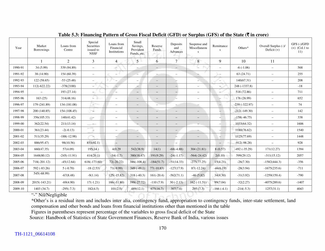
170

Table 5.3: Financing Pattern of Gross Fiscal Deficit (GFD) or Surplus (GFS) of the State (`̀̀̀ in crore)

Year Market

Borrowings

Loans from

Centre

Special

Securities

issued to

NSSF

Loans from

Financial

Institutions

Small

Savings,

Provident

Funds, etc.

Reserve

Funds

Deposits

and

Advances

Suspense and

Miscellaneou

s

Remittance

s Others*

Overall Surplus (-)/

Deficit (+)

GFS (-)/GFD

(+) (Col.1 to

11)

1 2 3 4 5 6 7 8 9 10 11

1990-91 34 (5.99) 539 (94.89) – – – – – – – -6 (-1.06) – 568

1991-92 38 (14.90) 154 (60.39) – – – – – – – 63 (24.71) – 255

1992-93 122 (58.65) -53 (25.48) – – – – – – – 140(67.31) – 208

1993-94 112(-622.22) -378(2100) – – – – – – – 248 (-1337.8)

-18

1994-95 – 193 (27.14) – – – – – – – 518 (72.86) – 711

1995-96 163 (25) 314(48.16) – – – – – – – 176 (26.99) – 652

1996-97 179 (241.89) 134 (181.08) – – – – – – – -239 (-322.97) – 74

1997-98 200 (140.85) 154 (108.45) – – – – – – – -212(-149.30) – 142

1998-99 356(105.33) 140(41.42) – – – – – – – -158(-46.75) – 338

1999-00 362(22.54) 211(13.14) – – – – – – – 1033(64.32) – 1606

2000-01 361(23.44) -2(-0.13) – – – – – – – 1180(76.62) – 1540

2001-02 511(35.29) -188(-12.98) – – – – – – – 1125(77.69) – 1448

2002-03 886(95.47) 98(10.56) 855(92.1) – – – – – – -912(-98.28) – 928

2003-04 660(47.35) 57(4.09) 195(14.) 4(0.29 542(38.9) 14(1) -68(-4.88) 304 (21.81) 8 (0.57) -492 (-35.29) 171(12.27) 1394

2004-05 1648(80.12) -245(-11.91) 414(20.1) -34(-1.7) 380(18.47) 191(9.29) -24(-1.17) -564(-24.42) 2(0.10) 599(29.12) -311(15.12) 2057

2005-06 718(-201.12) -45(12.64) 618(-173.60) 72(-20.22) 386(-108.4) -184(51.7) -51(14.33) -275(77.25) 15(4.21) -26(7.30) -1582(444.3) -356

2006-07 592 (-83.26) 5 (-0.70) -18 (2.53) 71(-9.99) 349 (-49.1) 77(-10.83) -127(17.9) 87(-12.24) -44(6.19) -28(3.94) -1675(235.6) -711

2007-08 545(-68.99)

-67(8.48) -9(1.14) 125(-15.82) 318 (-40.3) 161(-20.4) -562(71.1) -46 (5.82) 34(4.30) -31(3.92) -1259(159.4) -790

2008-09 2015(-143.21) -69(4.90) 17(-1.21) 166(-11.80) 390(-27.72) -110 (7.9) 30 (-2.13) 162 (-11.51) 99(7.04) -32(2.27) -4075(289.6) -1407

2009-10 1403 (34.7) -295(-7.3) 182(4.5) 101(2.5) 489(12.1) 675(16.7) 307(7.6) 295 (7.3) –166 (-4.1) -214(-5.3) 1257(31.1) 4043

“-” Nil/Negligible

*Other’s is a residual item and includes inter alia, contingency fund, appropriation to contingency funds, inter-state settlement, land

compensation and other bonds and loans from financial institutions other than mentioned in the table

Figures in parentheses represent percentage of the variables to gross fiscal deficit of the State

Source: Handbook of Statistics of State Government Finances, Reserve Bank of India, various issues

TH-1121_06614108

171

It is evident from table 5.3 that net loans available from the centre were the main sources of

financing gross fiscal deficit of the state during 1990s. The share of the net loans provided by

the central government has declined during the period of study which is found to be replaced

by market borrowings. The decline in the share of central government’s loans was mainly

due to declaration of the state as a special category state which helped it to acquire more plan

assistance in the form of grants which were earlier provided as loans (Srivastava et al., 1999).

The automatic entitlement of states to loans against small savings is also found to be

responsible for the declining share of central loans (Rajaraman et al., 2005). With the change

in the accounting system with effect from 1999-2000, states’ share in small savings which

was earlier included under loans from the Centre was included under internal debt and shown

as special securities issued to National Small Savings Fund (NSSF) of the Central

Government (RBI, 2011). As discussed above, the recommendation of the Twelfth Finance

Commission to prevent the Planning Commission from providing loans to the state

government also contributed towards reduction of central loans (Government of Assam,

2010). As a result of those changes, market borrowings have emerged as a significant source

of financing fiscal deficit of the state in recent times. During the first decade of the present

century, market borrowing was found to be the major source of financing the gross fiscal

deficit. Another significant source of borrowing for the government in recent years is the

small savings and provident funds of the state government. It can be inferred from the above

table that the existence of fiscal surplus has helped the states to repay the loans which in turn

lead to decline in the debt-GSDP ratio of the state. This happened in the year 2006-07, 2007-

08 and 2008-09. But the huge fiscal deficit in the year 2009-10 has again raised the question

of fiscal and debt sustainability of the state. As in any study of fiscal sustainability, primary

deficit is always the key policy variable, it is necessary to study the trend and composition of

primary deficit in the state which is carried out in the next sub-section.

5.2.4 Trend and Composition of Primary Deficit and Primary Revenue Deficit:

Primary deficit is that part of fiscal deficit which is net of interest payments. It represents the

gap in resources for meeting the current obligations. The decomposition of primary deficit

into primary revenue deficit and capital expenditure (including loans and advances) would

indicate the quality of deficit and sustainability of the fiscal stance of a state. The primary

TH-1121_06614108

172

revenue deficit which is calculated by deducting interest payments from revenue deficit

measures the extent to which the additional debt build-up in the current year, independent of

interest on inherited debt, is going towards current expenditures rather than towards build up

of assets through the capital account. Primary revenue deficit is considered as the first

sustainability indicator as it constitutes the floor of the overall primary deficit. The time

series data on trend and composition of primary deficit and primary revenue deficit of the

state are shown in table 5.4.

Table 5.4

Trend and Composition of Primary Deficit and Primary Revenue Deficit of the

State (`̀̀̀ in crore)

Year Non Debt

Receipt

Primary Revenue

Expenditure

Loans &

Advances

Capital

Outlay

Primary

Expenditure

Primary Revenue

Deficit Primary Deficit

1 2 3 4 5 6

(3+4+5) 7

8

(6-2)

1990-91

1783 1657 183 247 2087 -120 304 (2.86)

1991-92 2424 2055 245 285 2585 -363 161 (1.35)

1992-93 2619 2040 140 237 2417 -573 -202 (-1.54)

1993-94 3324 2411 153 251 2815 -907 -509 (3.36)

1994-95 2968 2682 131 277 3090 -279 122 (.78)

1995-96 3384 3088 160 301 3549 -288 165 (1.03)

1996-97 3864 3011 124 242 3377 -845 -487 (2.95)

1997-98 4335 3400 109 329 3838 -926 -497 (2.98)

1998-99 4518 3895 76 364 4335 -612 -183 (1.10)

1999-00 4855 4890 133 483 5506 49 651 (1.86)

2000-01 5656 5552 217 562 6331 -86 675 (1.83)

2001-02 5994 5784 82 513 6379 -181 385 (1)

2002-03 6821 5868 131 506 6505 -925 -316 (.72)

2003-04 7805 7004 128 622 7754 -761 -51 (.10)

2004-05 11326 8825 974 2181 11980 -1112 654 (1.24)

2005-06 12083 9026 106 1085 10217 -3019 -1866 (3.22)

2006-07 13702 9941 81 1453 11475 -3726 -2227 (3.45)

2007-08 15365 11232 143 1688 13063 -4093 -2302 (3.21)

2008-09 18112 12650 89 2373 15112 -5427 -3000 (3.24)

2009-10 19917 19399 99 2629 22127 -485 2210 (3.16)

Figures in parentheses represent percentage of these variables to GSDP at current prices.

(-) implies surplus

Source: Report of the Comptroller and Auditor General of India, Government of Assam, Various issues

TH-1121_06614108

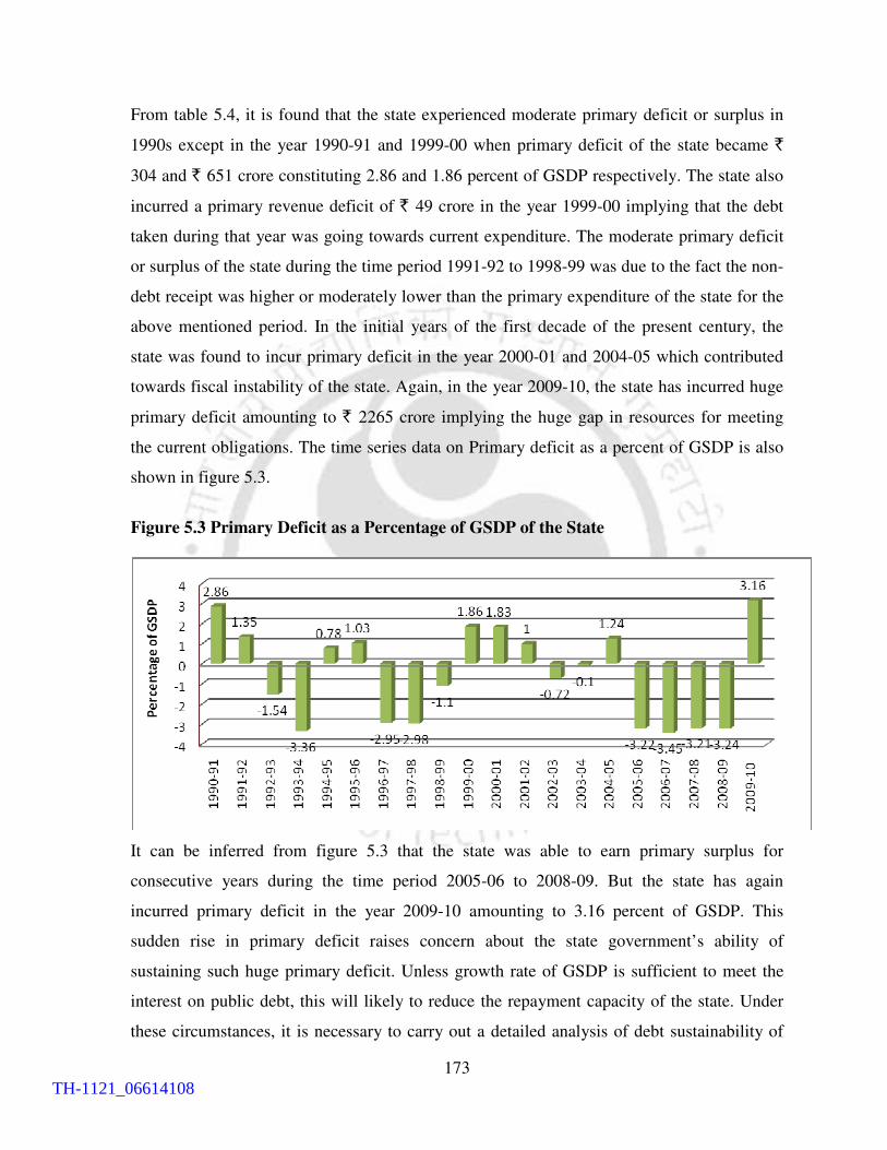
173

From table 5.4, it is found that the state experienced moderate primary deficit or surplus in

1990s except in the year 1990-91 and 1999-00 when primary deficit of the state became `

304 and ` 651 crore constituting 2.86 and 1.86 percent of GSDP respectively. The state also

incurred a primary revenue deficit of ` 49 crore in the year 1999-00 implying that the debt

taken during that year was going towards current expenditure. The moderate primary deficit

or surplus of the state during the time period 1991-92 to 1998-99 was due to the fact the non-

debt receipt was higher or moderately lower than the primary expenditure of the state for the

above mentioned period. In the initial years of the first decade of the present century, the

state was found to incur primary deficit in the year 2000-01 and 2004-05 which contributed

towards fiscal instability of the state. Again, in the year 2009-10, the state has incurred huge

primary deficit amounting to ` 2265 crore implying the huge gap in resources for meeting

the current obligations. The time series data on Primary deficit as a percent of GSDP is also

shown in figure 5.3.

Figure 5.3 Primary Deficit as a Percentage of GSDP of the State

It can be inferred from figure 5.3 that the state was able to earn primary surplus for

consecutive years during the time period 2005-06 to 2008-09. But the state has again

incurred primary deficit in the year 2009-10 amounting to 3.16 percent of GSDP. This

sudden rise in primary deficit raises concern about the state government’s ability of

sustaining such huge primary deficit. Unless growth rate of GSDP is sufficient to meet the

interest on public debt, this will likely to reduce the repayment capacity of the state. Under

these circumstances, it is necessary to carry out a detailed analysis of debt sustainability of

TH-1121_06614108

174

the state to find out whether difference between growth rate of GSDP and interest rate on

public debt is adequate to cancel out the effects of primary deficit.

5.3 Sustainability of Public debt in Assam:

Public debt is the accumulated stock of government financial liabilities. It is measured by

summing the face value of that stock (Rajaraman et al. 2005). In Indian context, public debt

refers to all financial liabilities of the government, irrespective of whom they are owed

(Lahiri and Kannon, 2004) A large accumulation of public debt may create problem for the

state government in terms of repayment of the principal and interest payments. It also raises

the issue of sustainability of the current stock of debt of the state. Sustainability is the

capacity to endure without breaking down. In the context of public debt, sustainability

embodies concern about the ability of the government to service its debt. A government

which does not generate enough current revenues for debt service must either default on its

obligations or borrow more to service its past debt as well as to cover ongoing imbalances.

Continual borrowings of this kind are known as ponzi game which is reflected in the time

path of debt-GSDP ratio. Usually, sustainability is measured in terms of debt-GSDP ratio.

Generally, low debt-GSDP ratio is desirable as it indicates an economy that produces a large

number of goods and services and probably profits that are high enough to pay back debts.

There is no universally prudent target value of debt-GSDP ratio (Chelliah, 2002; Buiter and

Patel, 1992). Sustainability implies maintaining a stable debt-GSDP ratio over a period of

time. Theoretical literature states that existence of primary deficit or surplus has a close

relation in maintaining a stable debt-GSDP ratio (Rath, 2005; Rajaraman, 2005). If a

particular government fails to meet the repayment obligations of the public debt, it will lose

its credibility in the debt market. This is very relevant as loans from market are found to be a

significant source of borrowings of the state government during the period of study. It is in

this context that the issue of sustainability of the public debt in the state has gained its

relevance in fiscal literature. The simplest way for determining the sustainability of debt of

the states has been to arrive at the acceptable level of debt-GSDP ratio and the ratio of

interest payments to total revenue receipts. It is very difficult to set a debt-GSDP ratio which

is likely to be sustainable. The Twelfth Finance Commission of Government of India

TH-1121_06614108

175

recommended 28 percent and 15 percent as acceptable level of the debt-GSDP ratio and the

ratio of interest payments to total revenue receipts respectively. The time series data on

outstanding liabilities, debt-GSDP ratio and interest payments-revenue receipt ratio of the

state government have been provided in table 5.5.

Table 5.5

Outstanding Liabilities, Debt to GSDP and Interest payments to Revenue Receipts

ratio of the State (`̀̀̀ in crore)

Year Outstanding

Liabilities

Debt-GSDP

ratio

Interest payments-

Revenue Receipt ratio

1 2 3 4

1990-91 4341 40.87 14.80

1991-92 4658 39.31 3.85

1992-93 4670 35.79 15.73

1993-94 4675 30.87 14.77

1994-95 5228 29.79 19.89

1995-96 6326 32.59 14.45

1996-97 6402 30.46 14.52

1997-98 6469 28.37 14.77

1998-99 6765 26.47 11.56

1999-00 8666 24.88 19.75

2000-01 10227 27.78 15.35

2001-02 11988 31.29 17.80

2002-03 13099 30.18 18.32

2003-04 15688 33.16 18.62

2004-05 17043 31.92 14.12

2005-06 18401 30.99 12.54

2006-07 19490 30.13 11.09

2007-08 20192 28.41 9.87

2008-09 22900 28.88 8.80

2009-10 27385 29.61 9.14

Source: State Finances: A Study of Budgets, RBI, various issues

It is evident from table 5.5 that the outstanding liabilities of the state government have

increased from ` 4341 crore in 1990-91 to ` 27385 crore and thus registering an annual

compound growth rate of 10.18 percent during that period. The debt-GSDP ratio of the state

TH-1121_06614108

176

was found to decline from 40.87 percent in 1990-91 to 24.88 percent in 1999-00. Since then,

the debt-GSDP ratio started increasing and in the year 2003-04, total outstanding debt of the

state government constituted 33.16 percent of GSDP. The state government faced the

problem of fiscal instability3

during this period, i.e. 1999-00 to 2004-05. This is due to the

fact that along with the high debt-GSDP ratio, the fiscal indicators of the state were found to

deteriorate during that period. But, in spite of high debt-GSDP ratio, the state government

was able to maintain a stable fiscal position during the time period 2005-06 to 2008-09

mainly due to the revenue and primary surplus attained by the state during that period. The

fiscal instability of the state during the time period 1999-00 and 2004-05 prompted to adopt

lots of fiscal reform measures which actually helped to maintain stable fiscal position. The

debt-GSDP ratio of the state was found to decline from 33.16 percent in 2003-04 to 29.61

percent in 2009-10. However, this ratio in 2009-10 is higher than the level prescribed by the

Twelfth Finance Commission. But it has been found to be lower than the sustainable level of

debt-GSDP ratio as computed from the theoretical model provided in section 5.1. The

sustainable level of debt-GSDP ratio for the state in the year 2009-10 is 32 percent as given

below:

It is also found that interest payments-revenue receipts ratio of the state is below the level as

recommended by the Twelfth Finance Commission. The diagrammatic representation debt-

GSDP ratio of the state has been shown in figure 5.4.

Debt 1+g Fiscal Deficit =

GSDP g GSDP

( )1 .14

.32= .04.14

+

TH-1121_06614108

177

Figure 5.4 Debt-GSDP ratio of the State

It is evident from figure 5.4 that the state has experienced significant improvement in the

debt- GSDP ratio during the period of study. Two main factors are found to contribute

towards decline in the debt-GSDP ratio of the state. As discussed in the previous sections, the

declaration of the state as a special category state helped the state to receive more grants from

the Planning Commission which were earlier provided as loans. The fiscal reform measures

adopted by the state government after the fiscal crisis in the later part of 1990s also helped

the state to reduce the debt-GSDP ratio of the state. As state government has adopted

different fiscal reform measures during that time period, it is necessary to analyze the

implication of those reform measures on the debt-GSDP ratio of the government.

5.3.1 Fiscal Reforms and Debt Status of the Government:

The continuous fiscal imbalances from 1999-00 prompted the State Government to undertake

different fiscal reforms measures targeting specifically the deficit indicators. The Eleventh

Finance Commission of Government of India fixed cumulative improvement in the reduction

of revenue deficit as proportion of revenue receipts at 16 percentages for special category

states like Assam during the award period of Eleventh Finance Commission. As against the

target of 16 percent, Government of Assam achieved 18 percent cumulative improvement in

reduction of revenue deficit as a percentage of revenue receipts. As a result, Government of

Assam was able to receive ` 159.45 crore as non-plan revenue deficit grant from the

incentive fund under Fiscal Reform facility of the Eleventh Finance Commission

TH-1121_06614108

178

(Government of Assam, 2011). Further, in pursuance of the award of the Twelfth Finance

Commission, Government of Assam enacted Assam Fiscal Responsibility and Budget

Management Act (AFRBM), 2005 to qualify for debt relief. As discussed in the previous

chapter, the main objective of the AFRBM Act was to reduce the revenue deficit to zero and

fiscal deficit to 3 percent of GSDP gradually by 2008-09 from the initial award period of

Twelfth Finance Commission. With the implementation of the AFRBM Act and adoption of

the Medium Term Fiscal Reform Plan under the Asian Development Bank funded Assam

Governance and Public Resource Management Programme (AGPRMP), Government of

Assam achieved the fiscal targets of AFRBM Act in the initial years of the Twelfth Finance

Commission award period. The revenue deficit, which was ` 292 crore in the year 2004-05,

became surplus of ` 1509 crore in 2005-06, ` 2210 crore in 2006-07, ` 2581 crore in 2007-

08, ` 3834 crore in 2008-09 respectively. Similarly, fiscal deficit, which was ` 2057 crore in

2004-05 turned into surplus of ` 356 crore in 2005-06, ` 711 crore in 2006-07, ` 790 crore

in 2007-08 and ` 1407 crore in 2008-09. As an incentive under the Debt Consolidation and

Reform Facility (DCRF) of the Twelfth Finance Commission, Government of Assam

received debt waiver of ` 105.41 crore for the year 2005-06 in 2007-08, ` 105.41 crore for

the year 2006-07 in 2008-09 and ` 105.41 crore for the year 2007-08 in 2009-10. Thus,

adoption of fiscal reform measures has helped the state to restrict the deficit indicators and

gain from different incentive schemes of the central government.

As discussed in the previous sections, primary deficit is a key policy variable which actually

helps to control the debt-GSDP ratio of the state. But along with primary deficit, growth rate

of GSDP and average interest payments are considered as critical variables for any study of

debt sustainability. Under these circumstances, it is necessary to examine the relationship

between these variables and see how it helps to control the debt-GSDP ratio of the state.

5.3.2 Primary Deficit and Sustainability of the Public Debt in Assam:

The sustainability of the current stock of debt is the main determinant of the overall fiscal

sustainability of a government (Hamilton and Flavin, 1986). Debt sustainability is defined as

the ability to maintain the constant debt-GSDP ratio over a period of time (Rajaraman et al.,

2005). In simple terms, public debt is considered to be sustainable as long as the growth of

TH-1121_06614108

179

income exceeds the interest rate or cost of public borrowings subject to the condition that the

primary balance is either positive or zero. The relationship between primary deficit and

public debt of the state as provided in the Domar model is discussed in section 5.1. A zero

primary deficit is required for stabilization of debt as percent of GSDP, if the nominal rate of

growth of GSDP is equal to the interest rate on inherited debt. Given the rate spread (GSDP

growth rate-interest rate) and quantum spread, debt sustainability condition states that if

quantum spread together with primary deficit is zero, debt-GSDP ratio would be constant or

debt would stabilize eventually. On the other hand, if the primary deficit along with quantum

spread is negative, debt-GSDP ratio would be rising and in case it is positive, debt-GSDP

ratio would eventually be falling (Rath, 2005; Domar, 1944). If there is a primary deficit, it is

likely that the debt-GSDP ratio will be higher at the close of the fiscal year, unless the growth

rate of GSDP during the year is higher than the nominal rate of interest on the inherited debt

stock. Additionally, the quantum spread and debt stabilization index are computed to know

the impact of the primary deficit and public debt on debt-GSDP ratio of the state. The

quantum spread is calculated by multiplying the rate spread with outstanding stock of debt.

The interest rate used here is the effective interest rate which is calculated as,

Interest PaymentsEffective interest rate = * 100

Amount of previous year's fiscal liabilities + current year's fiscal liabilities

2

The debt stabilization index is nothing but the summation of the quantum spread and the

primary deficit. A positive debt stabilization index helps to reduce the debt-GSDP ratio and

vice versa (Rath, 2005). The debt sustainability status of the state in terms of interest spread

and quantum spread during the study period has been shown in table 5.6.

Table 5.6 reveals that the state had a very high debt-GSDP ratio in the year 1991-92 (39.31

percent). However, there was a gradual decline of the ratio till 1999-00 when the ratio was

found to be 24.88 percent. The positive rate spread or Domar gap enjoyed by the state in

some years during the above time period might have helped to reduce the debt-GSDP ratio.

The primary surplus experienced by the state in some of the years such as 1992-93, 1993-94,

1996-97, 1997-98 and 1998-99 also contributed towards the favourable debt-GSDP ratio of

the state. The debt-GSDP ratio of the state, however, was found to increase from the year

2000-01 and reached a high of 33.16 percent in 2003-04. The state had experienced primary

TH-1121_06614108

180

deficit for consecutive years during the period from 1999-00 to 2001-02 which actually

contributed towards increased debt-GSDP ratio.

Table 5.6

Debt Sustainability of Assam in terms of Quantum Spread and Primary Deficit (`̀̀̀ in crore)

Year

GSDP Growh

Rate(at

Current

Prices)

Effective

Interest

Rate

Rate

Spread

Quantum

Spread

(Dt*Rate

spread)

Primary

Deficit(-)

Debt Stabilization

Index(quantum

spread+primary

deficit)

Debt-GSDP

ratio

1 2 3 4 5 6 7 8

1991-92 11.56 2.07 9.49 550 -162 388 39.31

1992-93 10.13 8.81 1.31 76 203 279 35.79

1993-94 12.79 10.34 2.46 139 508 647 30.87

1994-95 15.90 11.90 4.01 253 -121 132 29.79

1995-96 10.60 8.45 2.15 165 -165 0 32.59

1996-97 8.27 8.80 -0.53 -41 486 445 30.46

1997-98 8.51 9.93 -1.42 -111 497 386 28.37

1998-99 12.07 7.87 4.19 343 183 526 26.47

1999-00 14.50 11.44 3.06 270 -650 -380 24.88

2000-01 5.69 9.16 -3.47 -361 -675 -1036 27.78

2001-02 4.07 9.56 -5.49 -669 -386 -1055 31.29

2002-03 13.30 9.93 3.37 449 317 766 30.18

2003-04 8.98 10.05 -1.07 -170 52 -118 33.16

2004-05 11.05 8.51 2.54 433 -654 -221 31.92

2005-06 11.21 8.52 2.69 495 1866 2361 30.99

2006-07 8.94 8.00 0.94 182 2227 2409 30.13

2007-08 9.87 7.62 2.25 454 2302 2756 28.41

2008-09 14.27 7.39 6.88 1575 3000 4575 28.88

2009-10 (R.E) 13.85 7.29 6.56 1797 -2210 -413 29.61

Source: Author’s own calculation based on the report of the Comptroller and Auditor

General of India, Government of Assam, various issues and GSDP data from CSO reports)

The unfavourable rate spread also contributed towards increase in debt-GSDP ratio of the

state. The state has been able to maintain a stable debt-GSDP ratio in recent years. This is

mainly due to the higher growth of GSDP compared to effective interest rate on public debt.

The growth rate of GSDP is found to be greater than the effective interest rate on public debt

for consecutive years from 2004-05 to 2009-10. The occurrence of primary surplus in some

years also helped to keep the debt-GSDP ratio at a stable level. The debt stabilization index

alternates its sign during the period under study and thus helped to maintain a stable debt

TH-1121_06614108

181

path. But the debt stabilisation index is found to be negative in the year 2009-10 implying

that debt GSDP ratio may increase in near future. This is mainly due to the fact that the state

incurred the highest ever primary deficit of ` 2210 crore in the year 2009-10. The positive

difference between the growth rate and interest rate is found to be insufficient to cancel out

the effects of primary deficit. As a result, the debt stabilisation index is found to be negative

for the year 2009-10. There is a need, on the part of the state government, to take corrective

measures to keep the debt path at sustainable level. Otherwise, the state government has to

borrow more to discharge the debt obligation in terms of payment of principal and interest

obligation. This may also create the problem of lack of availability of funds for other

activities such as capital expenditure for asset creation and other purposes. This actually

leads to increase in public debt of the state. This cannot be allowed to continue forever as this

may push the state into an unsustainable debt path. Under these circumstances, it is necessary

to make a long term analysis of fiscal and debt sustainability of the state by taking the

relevant variables into consideration.

5.4 Long term Analysis of Fiscal and Debt Sustainability of the State:

From the above analysis, some conclusions regarding sustainability of the fiscal position of

the state may be drawn from the indicators such as composition and nature of the fiscal and

primary deficit, rate spread and debt stabilization index etc. The conclusions based on those

analyses provide an idea of sustainability for a particular period of time. To be able to draw

inferences in a rigorous manner, more sophisticated tools such as time series analysis needs

to be applied covering the whole time period taken for the analysis. Thus, cointegration

analysis has been carried out to examine the long term association among the fiscal variables

in the state for the period 1990-91 to 2009-10.

The idea behind carrying out cointegration analysis is to examine whether the state has

maintained the inter-temporal budget constraint during the period of study. The intertemporal

budget constraint tests of sustainability of fiscal policy asks whether past behavior of

revenue, expenditure and fiscal deficits could be continued indefinitely without prompting

adverse response from the lenders (Olekalns and Cashin, 2000).

TH-1121_06614108

182

Now, the rationale behind the model is that the inter-temporal budget constraint, under the

no-Ponzi scheme rule, imposes restrictions on the time series properties of government

revenue and expenditure. For sustainability of the current stock of debt, the government

expenditure and revenue must be stationary at least in the first difference. The stationary

property restricts the extent to which government expenditure and revenue can deviate from

each other over time. In particular, if government expenditure and revenue is integrated of

order 1, they may be cointegrated (Gujarati, 2004). Cointegration implies that there exists an

error correction mechanism pushing government finances towards the levels required by the

intertemporal budget constraint. Lack of cointegration among the variables implies that under

unchanged fiscal policies, the debt stock of the state government is unsustainable.

Cointegration is a two step procedure where value of the residual has to be calculated from

the regression of the relevant variables. If the residual obtained from the regression are found

to be stationary, then the variables are said to be cointegrated (Gujarati, 2004).

In the current analysis, time series data on revenue receipts and revenue expenditure as well

as revenue receipt and total expenditure of the state are considered. The rationale behind

taking revenue receipt and revenue expenditure as the relevant variable is that imbalances

between the two variable have an impact on fiscal deficit of a state. As discussed in the

previous section, an increase in revenue deficit has an implication for the debt stock of the

government as it leads to increase in fiscal deficit of the state. Similarly, long run association

between revenue receipts and total expenditure helps in ensuring fiscal stability of the state.

Following Hakkio and Rush (1991) and Olekalns and Cashin (2000),

sustainability of debt stock can be evaluated by estimating the following two log-linear

regressions -

( )t o 1 t tLn RR = α + α Ln RE +U …………………....... 1

( )t o 1 t tLn RR β β Ln TE +V ....... 2= + …………………

Here, RR = Revenue Receipt

RE = Revenue Expenditure

TE = Total Expenditure

TH-1121_06614108

183

U = Random disturbance or error term in regression equation (1)

V = Random disturbance or error term in regression equation (2)

The necessary conditions for the existence of cointegration is that the individual series are

integrated of order one. Should only one of the series is I (1), with the other being stationary,

the two series will permanently diverge and equation (1) and (2) will not hold (Olekalns and

Cashin, 1999). Initially, the time period taken for the analysis is from 1990-91 to 2009-10.

The variables are found to be integrated of order 1. But the R2 values of the error correction

variables are found to be very less and values of the F- statistic obtained from the regression

analyses are found to be insignificant even at the 10 percent level. This may be due to less

number of observations, not considered to be sufficient for time series models. To facilitate

better treatment of the models, the analysis has been reworked by taking a few more years in

to consideration. Accordingly, the two time series models have taken in to account the time

period of 1980-81 to 2009-10.

As the variables are in current prices, they are converted in to constant 2004-05 prices by

using the GSDP price deflator. The GSDP price deflator is computed as a ratio of current to

constant prices as done in the previous chapters. Now, Dickey Fuller unit root test is used to

determine the order of integration where null hypothesis is that respective series have a unit

root. The results of the Dickey Fuller unit root test have been provided in table 5.7.

TH-1121_06614108

184

Table 5.7

Dickey Fuller test for Unit Root for Revenue Receipt, Revenue Expenditure and Total

Expenditure (For the Time Period 1980-81 to 2009-10)

Test

Statistic

(t)

1% critical

Value

5% critical

value

10% critical

value

Mackinnon

approximate p value

Ln RR 0.150 -3.723 -2.989 -2.625 0.9693

Ln RE 0.329 -3.750 -3.00 -2.630 0.9962

Ln TE 0.497 3.723 2.989 2.625 0.9962

Using Difference Operator

Ln RR -8.196 -3.750 -3.00 -2.630 0.000

Ln RE -4.323 -3.750 -3.00 -2.630 0.004

Ln TE -5.356 -3.730 -2.992 -2.626 0.0033

From table 5.7, it is clear that all the variables are integrated of order one. In other words,

there may be cointegration relationship between these variables. If they are co-integrated, it

implies that there is a long term relationship between the two variables and fiscal position of

the state is sustainable during that period. For this, the values of the residuals Ut and Vt have

to be computed from equation (1) such that

� ( )t o 1 tU Ln RR α α Ln RE ..... 3= − − ………………………

� ( )t t o 1 tV Ln RR β β Ln TE ..................................... 4= − −

Now, cointegration requires that the residuals obtained from the equation (3) and (4) be

stationary. The standard way of testing whether this requirement is met by the data is to use

the Dickey Fuller test of unit root. But since the estimated Ut and Vt are based on the

estimated cointegrating parameter α1 and β1 respectively, Dickey Fuller critical significant

values are not quite appropriate (Gujarati, 2004). Engle and Granger (1987) have calculated

the critical values of the test. This involves estimating autoregressive parameter from the

“second stage” regression.

( )t 1 t-1U = þ U + €t.................................................. 5

( )t 2 t 1 V þ V t ........................ 6 ϑ−

= + ………………

Here, €t and ϑt are the random error terms,

TH-1121_06614108

185

þ1 and þ2 are the parameters to be estimated in the model.

if |þ1| < 1, then there is a cointegrating relationship between revenue receipt and revenue

expenditure.

Similarly, if |þ2| < 1, then there is a cointegrating relationship between revenue receipt and

total expenditure.

The results of the Engle and Granger cointegration test have been provided in table 5.8 and

5.9.

Table 5.8

Engle-Granger Test of Cointegration between Revenue Receipt and Revenue

Expenditure

Variable Test Statistic

(t)

1% critical

Value

5% critical

value

10% critical

value

Ut -4.923 -3.679 -2.968 -2.623

Table 5.9

Engle-Granger Test of Cointegration between Revenue Receipt and Total Expenditure

Variable Test Statistic

(t)

1% critical

Value

5% critical

value

10% critical

value

Vt

-7.600 -3.689 -2.972 -2.625

As computed test statistic of both the error terms in absolute value are found to be greater

than Engle Granger critical value at 1 percent level, residuals are integrated of order 0 i.e.; I

(0). In other words, although the variables are non-stationary, the residuals obtained from

their regression are stationary. It implies that, there is a long term association among the

variables, revenue receipt and revenue expenditure as well as revenue receipts and total

expenditure.

The above cointegration analyses show the long run relationship among the variables. But

along with the cointegration, it is also necessary to examine short term behaviour of the

variables. Keeping this fact in mind, the error correction mechanism (ECM) is also

incorporated in this analysis to examine short term behaviour among the variables. This test

TH-1121_06614108

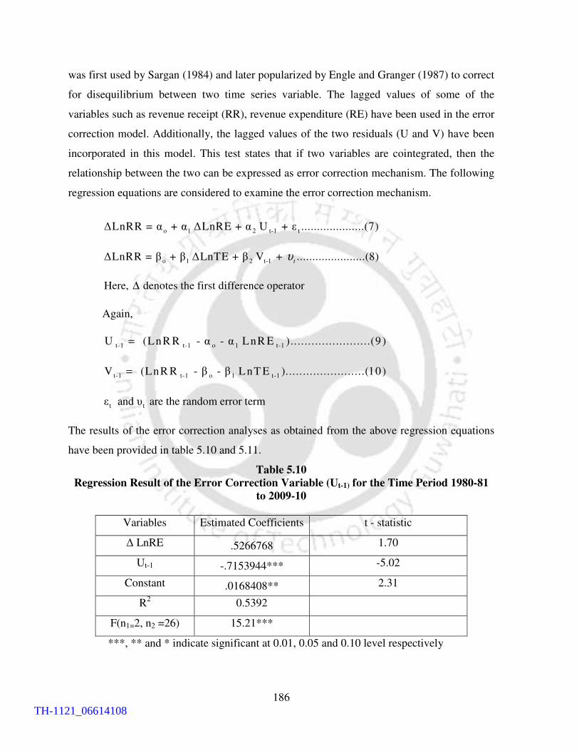
186

was first used by Sargan (1984) and later popularized by Engle and Granger (1987) to correct

for disequilibrium between two time series variable. The lagged values of some of the

variables such as revenue receipt (RR), revenue expenditure (RE) have been used in the error

correction model. Additionally, the lagged values of the two residuals (U and V) have been

incorporated in this model. This test states that if two variables are cointegrated, then the

relationship between the two can be expressed as error correction mechanism. The following

regression equations are considered to examine the error correction mechanism.

o 1 2 t-1 t∆LnRR = α + α ∆LnRE + α U + ε ....................(7)

o 1 2 t-1∆LnRR = β + β ∆LnTE + β V + ......................(8)t

υ

Here, denotes the first difference operator ∆

Again,

t-1 t-1 o 1 t-1U (LnR R - α - α LnR E ).......................(9 )=

t-1 t-1 o 1 t-1V (LnR R - β - β LnT E ).......................(10)=

t tε and υ are the random error term

The results of the error correction analyses as obtained from the above regression equations

have been provided in table 5.10 and 5.11.

Table 5.10

Regression Result of the Error Correction Variable (Ut-1) for the Time Period 1980-81

to 2009-10

Variables Estimated Coefficients t - statistic

∆ LnRE .5266768 1.70

Ut-1 -.7153944*** -5.02

Constant .0168408** 2.31

R2 0.5392

F(n1=2, n2 =26) 15.21***

***, ** and * indicate significant at 0.01, 0.05 and 0.10 level respectively

TH-1121_06614108

187

Table 5.11

Regression Result of the Error Correction Variable (Vt-1) for the Time Period 1980-81

to 2009-10

Variables Estimated Coefficients t - statistic ∆ LnTE .4265848 2.14

Vt-1

-.7715409*** -5.54

Constant .0109217** 1.16 R

2

0.5586 F(n

1=2, n

2 =26) 16.45***

***, ** and * indicate significant at 0.01, 0.05 and 0.10 level respectively

It is evident from table 5.10 that the error correction variable (Ut-1) is found to be negative

and significant suggesting that deviation from equilibrium is corrected at 71 per cent per

year. Similarly, error correction variable (Vt-1

) as obtained from table 5.11 is also found to be

negative and significant. In other words, along with the long term association, there exists

short term association between these fiscal variables which actually helped the state to

maintain a stable fiscal position for most of the years taken for the analysis.

5.5 Conclusion:

It can be inferred from the above discussion that the state has been experiencing fluctuation

of fiscal deficit during the period of study. It has been observed that the occurrence of

revenue deficit has contributed towards increase in fiscal deficit of the state during the period

of study. As sustainability of the fiscal position of the state is mainly dependent on nature of

fiscal deficit, the higher proportion of revenue deficit to fiscal deficit led the state in to huge

fiscal imbalances in the later part of 1990s. The recent increase in revenue and fiscal deficit

of the state in the year 2009-10 is an area of concern for the state. The state government has

to take immediate corrective measures to restrict the fiscal deficit. The financing pattern of

gross fiscal deficit indicates the growing importance of market borrowings in economic

development of the state. Significant decline in the share of central government’s loans to the

state government has been observed during the period of study.

TH-1121_06614108

188

The sudden decline in the debt-GSDP ratio of the state during the first half of 1990s is

mainly due to the declaration of the state as a special category state. As loans from the central

government constitute the major portion of state’s debt during that period, the conversion of

the huge amount of loans in to grants helped the state tremendously to reduce the debt-GSDP

ratio. The state has been able to maintain a stable debt GSDP ratio in recent years mainly due

to positive interest spread enjoyed by the state. Along with that, primary surplus enjoyed by

the state during the period of study also contributed towards reduction of debt-GSDP ratio of

the state. The incentive provided by the Eleventh and Twelfth Finance Commission of India

and subsequent reform measures adopted by the state proved to be crucial in maintaining

stable fiscal position in the later part of the present decade.

The existence of cointegration between revenue receipt and revenue expenditure as well as

revenue receipt and total expenditure implies that the state has been able to maintain fiscal

sustainability during the period under study. Along with the long run relationship, short term

association among the variables has been observed as the error correction variables are found

to be negative and highly significant.

Notes:

1. Non-debt receipt includes revenue receipts, miscellaneous capital receipts and recovery of

loans and advances.

2. A government which does not generate enough current revenues for debt service must either

default on its obligations or borrow more to service its past debt as well as to cover ongoing

imbalances. Continued borrowings of this kind are known as ponzi game.

3. Fiscal instability is a situation of progressively increasing budget deficits which create

disruption in the normal functioning of the economy.

4. The theoretical model as explained in section 5.1 is mainly based on the papers by Rath

(2005), Rajaraman et al. (2005) and Lahiri and Kannon (2004) and Domar (1944).

****

TH-1121_06614108

189

CHAPTER 6

Summary of Findings, Conclusions and Policy Suggestions

The present study can be viewed as a research contribution to the effort to address the issue

of fiscal instability in the state and suggest policy measures to ensure fiscal stability with

proper allocation of resources for developmental activities. Before drawing the final

conclusion and working out the policy implications, it may be worthwhile to go over the

principal findings of the study. A summary of these findings is presented in the following

section.

6.1 Principal Findings:

1. Total revenue of the state government has increased from ` 1777 crore in 1990-91 to `

19884 crore 2009-10 registering 11.18 times increase during the period of study. The

compound annual growth rate of total revenue is found to be 13.55 percent during the period

of study. The compound annual growth rate of own tax revenue during the study period is

found to attain the highest value of 13.91 percent among the all categories of revenue. For the

same time period, non-tax revenue of the state has increased from ` 278 crore in 1990-91 to

` 2753 crore in 2009-10 with a compound growth rate of 12.83 percent. Similarly, shared

taxes and grants-in-aid have increased from ` 488 and ` 591 crore in 1990-91 to ` 5993 and

` 6805 crore respectively in 2009-10. The compound growth rate of these two sources of

revenue is found to be 13.42 percent and 13.72 percent respectively during the above

mentioned period.

2. Improvements in the revenue performance of the state has been observed during the time

period 2000-01 to 2009-10 compared to the time period 1990-91 to 1999-00 as compound

growth of the total revenue is found to be higher in the first decade of the present century

than the previous decade. The compound growth rate of tax and non-tax revenue of the state

is found to be 15.07 percent and 20.16 percent respectively during the time period 2000-01 to

2009-10 compared to 12.63 and 5.37 percent respectively in the previous decade. Similarly,

the growth rate of central transfers in terms of shared taxes and grants-in-aid has experienced

a growth rate of 13.71 and 14.46 percent respectively during the time period 2000-01 to

2009-10 compared to 12.85 and 12.62 percent respectively during 1990-91 to 1999-00.

TH-1121_06614108

190

3. The analysis has empirically established the dependence of the state government on central

transfers for its different activities. No significant improvement of the ratio of own revenue

to total revenue has been observed during the period of study implying the over dependence

of the state on central transfers for its developmental activities. On an average, central

transfers constitute more than 64 percent of the state’s total revenue receipt during the period

of study. Compared to that, the dependence of the non-special category states on central

transfers is found to be much less as central transfers, on an average, contribute only 35.02

percent of the total revenue receipt of those states during the period under consideration.

Similarly, dependence of the state on central transfers is found to be high than the all states

average for all the sub-periods taken for the analysis. Among the special category states, the

performance of Sikkim and Himachal Pradesh is found to be better than Assam for the last

three sub-periods taken for the analysis.

4. As the state is heavily dependent on central transfers for its developmental activities, the

change in the devolution criteria has a great bearing on fiscal stability of the state. The thrust

imposed by the recent Finance Commissions on efficiency criteria such as tax effort and

fiscal discipline along with the equity criteria is a step towards this direction. The state

government has to maintain a stable fiscal position to acquire benefit from the incentive

schemes of the central government.

5. Among the central transfers, grants-in-aid are found to be the major contributor of the total

revenue during the period of study constituting, on an average, 36.21 percent of the total

revenue receipt. The increased contribution of grants-in-aid is mainly due to declaration of

the state as a special category state in the year 1990-91. This initiative by the central

government enables the state to receive more grants from the Planning Commission.

6. Regarding shared taxes, introduction of the efficiency factors by the Finance Commissions

in their devolution formula is found to incentivize the state government to bring in more

efficiency in revenue collection. Increased efforts on the part of the state government have

been observed to reduce the arrear of collection and cost of collection of taxes and duties.

TH-1121_06614108

191

The improved buoyancy coefficients of own tax and non-tax revenue of the state government

in the last decade of the present century also signifies the increased effort of the government

to bring efficiency in revenue collection. Among the Finance Commissions transfers to the

state government, shared taxes constitute, on an average, 85.11 percent of the total transfers

during the period of study.

7. The grants from the Planning Commission to the state constitute, on an average, 62.31

percent of the total grants from the Central government during the period of study. The

Planning Commission’s grant to the state government is found to increase due to declaration

of the state as a special category state in the year 1990-91. As a result, share of grants for

state plans jumped from 41.86 percent of total grants in the year 1990-91 to 65.22 percent in

the 1991-92. In other words, declaration of the state as a special category state in 1990-91

actually helped the state to receive more grants from the Planning Commission in the

subsequent years.

8. The own tax revenue of the state government has contributed, on an average, 23.84 percent

of the total revenue receipt during the period of study. Sales tax is found to be the major

contributor of own tax revenue as it contributes, on an average, 67.80 percent of the total

own tax revenue compared to the all states average of 59.23 percent.

9. Decline in the growth rate of sales tax has been observed during the post VAT period

compared to the pre-VAT period as the average growth rate of sales tax during the period

2000-01 to 2004-05 was found to be 23.57 per cent while the growth rate for the period

2005-06 to 2009-10 was 11.28 per cent. Thus, the average growth rate of sales tax in the post

VAT period registered a decrease of 12.29 per cent.

10. Significant decline in the contribution of agriculture income tax has been observed during

the period of study as contribution of this source of revenue has declined from 21.46 percent

in 1990-91 to 1.56 percent in 2009-10. Agricultural income tax in the state comes mainly

from cultivation of tea. The decline in the share of the agricultural income tax is found to be

TH-1121_06614108

192

contributed by various factors such as disintegration of USSR, decline in the rate of

agricultural income tax etc.

11. The share of land revenue to own tax revenue of the state has declined from 3.15 percent

in the year 1990-91 to 2.35 percent 2009-10. Average contribution of land revenue to own

tax revenue of the state is found to be 4.84 percent during the period of study. The low rate of

land revenue is found to be the main reason for low and declining contribution of this source

of revenue.

12. The proceeds of excise duties in Assam have experienced erratic fluctuations with

periodic increase in its share. The later part of 1990s witnessed an increase in the share of

these components to over 10 percent of total own tax revenue followed by reduction in its

share in subsequent years. The compound growth rate of this source of revenue is found to be

16.5 percent during the study period which is higher than other sources of tax revenue.

13. The average contribution of stamp and registration and taxes and duties on electricity is

found to be very less as it contributed 2.74 percent and 0.50 percent of the own tax revenue

respectively during the period of study. On the other hand, average contribution of motor

vehicle tax and tax on passengers and goods is found to be 4.78 percent of the own tax

revenue during the period of study.

14. The asymmetries in the contribution of the different sources of own tax revenue of the

state government reflect the inability of the state government to utilize the other sources of

tax revenue except sales tax.

15. Similarly, own non-tax revenue of the state government is found to be mainly contributed

by the proceeds from the royalty on petroleum. The royalty on petroleum, on an average, has

contributed 75 percent of the total non-tax revenue of the state government. The contribution

of other sources of non-tax revenue is found to be insignificant during the period of study.

This signifies the inefficiency of the administrative machinery to collect revenue from the

other sources of non-tax revenue.

TH-1121_06614108

193

16. The tax-GSDP ratio of the state which is generally used as a proxy for tax effort is found

to be low compared to other major states average for the four sub-periods taken for the

analysis. But the ratio was found to be comparatively better than the average of the special

category states for the above mentioned period. The tax-GSDP ratio of the state is found to

be the lowest during the time period 1995-96 to 1999-00 amounting to 3.86 percent of the

GSDP. The low tax-GSDP ratio during that period is assessed from the fact that arrears of

revenue have increased tremendously from ` 160.50 crore in 1995-96 to ` 2784 crore in

2001-02. In other words, large arrears of revenue during that period may contribute towards

low tax to GSDP ratio of the state.

17. Fluctuation has been observed in the year wise buoyancy coefficients of own tax revenue,

non-tax revenue, sales tax and own revenue of the state during the period of study.

Improvement in the buoyancy coefficient of own tax, non tax, sales tax and total own

revenue of the state has been observed during the first decade of the present century than the

previous decade. The collection of huge arrear of revenue is found to contribute positively

towards increased collection of own revenue and in turn buoyancy coefficients of the state

government in the last decade of the present century. The buoyancy coefficients of own

revenue as computed by regressing all the four categories revenue to GSDP of the state are

found to be comparatively higher during the time period 2000-01 to 2009-10 compared to the

time period 1990-91 to 1999-00. The computed buoyancy coefficient of own tax, non tax,

sales tax and own revenue of the state are found to be less than 1 for all categories of revenue

during 1990s. But during the time period, 2000-01 to 2009-10, the buoyancy coefficients are

found to be positive and greater than one. The buoyancy of non-tax revenue is found to be

1.92 during the time period 2000-01 to 2009-10 implying a significant improvement over the

previous decade. Similarly, buoyancy of own tax, sales tax and own revenue is found to be

1.32, 1.43 and 1.51 during the first decade of the present century. In other words, buoyancy

coefficients of the revenues of the state government are found to be better during the first

decade of the present century.

18. Leakages in own revenue of the state has been observed during the period of study. The

state has been accumulating a large arrear of revenue particularly in the later part of the

TH-1121_06614108

194

1990s. The Finance department did not furnish data on accumulated arrear of revenue for

consecutive year from 1998-99 to 2000-01. This is a clear example of fiscal indiscipline on

the part of the state government. After that significant improvement has been observed in

collection of arrear of revenue which is found to be mainly contributed by two factors. The

computerization of administration department has helped to find out the defaulters. Similarly,

the audit report of the Comptroller and Auditor General of India in 2001-02 pointed out huge

uncollected arrear of revenue. This compelled the state government to take immediate

measures for collection of revenue. This also signifies the importance of the monitoring

agency in smooth functioning of a system.

19. The average cost of collection of the state’s taxes and duties is found to be comparatively

higher than the all state average cost of collection for most of the year taken for the analysis.

No clear trend has been observed regarding collection of revenue and cost of collection. It is

generally happens that average cost of collection declines with increase in collection. But no

such trend has been observed in case of Assam. The cost of collection of the major taxes in

Assam is also found to be comparatively higher than the all India average cost of collection.

This also signifies the low effort on the part of the administrative machinery to reduce the

cost of collection of the state tax revenue.

20. The cost recovery of different social and economic services of the state is found to be

comparatively less than all states recovery rate for most of the years taken for the analysis.

The average cost recovery of selected services such as education, medical and public health

and irrigation of the state during the period of study is found to be 0.60, 2.23 and 0.44

percent respectively compared to the all states average of 1.55, 5.46 and 11.20 percent

respectively. Similarly, the average cost recovery of aggregate social and economic services

of the state is found to be 0.96 and 11.32 percent respectively compared to the all states

average of 3.43 and 29.98 percent respectively during the study period.

21. The panel regression analysis between the per-capita own tax revenue and per capita own

GSDP for fifteen major states along with Assam has shown that Assam has underperformed

TH-1121_06614108

195

in terms of in terms of revenue effort compared to the average Indian states during the period

under consideration.

22. The composite index of revenue mobilization which is used to measure the relative

performance of the state within the period of study is found to be comparatively better in the

later part of the first decade of the present century than the previous decade. This confirms an

improvement in the fiscal position of the state in the first decade of the present century.

23. Increase in total and aggregate expenditure of the state has been observed during the

period of study. The average ratio of aggregate expenditure to GSDP of the state during the

study period is found to be higher compared to the ratio in 1980s. The aggregate expenditure

of the state government has increased from ` 2689 crore in 1990-91 to ` 24968 crore in

2009-10 and thus registered a growth rate of 12.44 percent during that period.

24. Similarly, total expenditure-GSDP ratio of the state has increased from 17.77 percent in

1990-91 to 25.91 percent in 2009-10. This signifies the applicability of the Wagner

hypothesis that “increase in GSDP leads to more than proportionate increase in the public

expenditure” of the state government. The total expenditure of the state government has

increased from ` 2350 crore in 1990-91 to ` 23960 crore in the year 2009-10 and has

registered a compound annual growth rate of 13 percent during that period. But the

compound growth rate of total expenditure during the time period 2000-01 to 2009-10 is

found to be 14.30 percent which is higher than the compound growth rate of the previous

decade.

25. It has been found that revenue expenditure constitutes the major portion of the total

expenditure of the state during the period of study ranging from 80.21 in 1991-92 to 92

percent in 2001-02. On an average, revenue expenditure constitutes 87.86 percent of the total

expenditure during the period of study leaving little fund available for capital expenditure

and advancement of loans and advances. Compared to that, revenue expenditure of all states,

on an average, constitutes 84.55 of the total expenditure during the period of study.

TH-1121_06614108

196

26. It has been found that expenditure on salary and wages, interest payments and pension

constitute the major portion of the revenue expenditure leaving little fund available for

expenditure on operation and maintenance. These three components of revenue expenditure,

on an average, have constituted 73.81 and 72.41 percent of revenue receipt and revenue

expenditure respectively during the time period 1990-00 to 2009-10.

27. Capital outlay and loans and advances as provided by the state government has

constituted 9.01 and 3.13 percent of the total expenditure respectively compared to the all

states average of 11.52 and 4 percent during the period of study. The low proportion of the

capital expenditure in total expenditure of the state signifies the inappropriate priority of the

state government for developmental activities.

28. Improvement in the ratio of capital outlay to capital expenditure has been observed

during the period of study implying that more funds will be available for developmental

activities rather than repayment of public debt. The proportion of capital outlay to capital

expenditure has increased from 32.12 percent in 1990-91 to 83.23 percent in 2009-10. The

expenditure on economic services is found to constitute the major portion of the expenditure

on capital outlay averaging 88.77 percent of the total capital outlay.

29. The increase in developmental expenditure of the state government during the study

period implies better quality of expenditure. The compound growth rate of development

expenditure of the state is found to be less than the compound growth rate of total and

aggregate expenditure during the period of study. The regression results confirms the less

than proportionate growth of development expenditure with respect to both total and

aggregate expenditure of the state.

30. The computed value of the expenditure management index of the state is found to be low

compared to the other developed states and all states average for both the sub-period

considered for the analysis i.e., 2000-01 to 2004-05 and 2005-06 to 2009-10. It implies that

overall management of expenditure of the state is not at par with the other developed states in

India. Slight improvement of the index for the state has been observed as the value of the

TH-1121_06614108

197

index has increased from .525 during the sub period 2000-01 to 2004-05 to .533 during 2005-

06 to 2009-10.

31. It is found that that imbalance between the revenue receipts and expenditure led the state

into fiscal imbalances during the time period 1999-00 and 2004-05. The increase in deficit

indicator of the state in the year 2009-10 is a matter of concern for the state. Timely steps are

required on the part of the state government to keep the deficit indicators under control.

32. The persistently large and fluctuating fiscal deficit of the state is found to create fiscal

instability during the period of study. The issue became more complex during the later part of

1990s and in the year 2009-10 as revenue deficit was found to contribute a significant portion

of the fiscal deficit. As the sustainability of the fiscal position of the state is mainly

dependent on nature of fiscal deficit, the higher proportion of revenue deficit to fiscal deficit

led the state into large fiscal imbalances in the later part of 1990s.

33. The financing pattern of gross fiscal deficit indicates the growing importance of market

borrowings in economic development of the state. Significant decline in the share of central

government borrowing has been observed during the period of study. This can be attributed

to some of the following:

(a) The state was declared as a special category state in the year 1990-91 which entitled the

state to secure Central assistance for the State Plans in the form of 90 percent as grants and

10 percent as loans.

(b) With the change in the accounting system with effect from 1999-2000, states’ share in

small savings which was included earlier under loans from the Centre is included under

internal debt and shown as special securities issued to National Small Savings Fund (NSSF)

of the Central Government.

(c) The policy of the central government to stop providing loans to the state government in

the later part of the first decade of the present century after the recommendation of the

Twelfth Finance Commission also contributes towards reduction of central loans. As a result

TH-1121_06614108

198

of those changes, a market borrowing has emerged as a significant source of financing fiscal

deficit of the state in recent years.

34. The declaration of the state as a special category states has helped the state to reduce its

debt-GSDP ratio during the first part of 1990s. It is found that the state has maintained a

constant debt-GSDP ratio in recent years mainly due to low growth of interest payments

compared to the growth of GSDP. The incentive taken by the Eleventh and Twelfth Finance

Commission of India and subsequent reform measures taken by the state actually has helped

the state to maintain stable fiscal position in the later part of the present decade.

35. The existence of cointegration between revenue receipt and revenue expenditure as well

as revenue receipt and total expenditure excluding interest payments implies that the state has

been able to maintain a sustainable fiscal policy during the period under study. The error

correction variables Ut-1 and Vt-1 are also found to be negative and significant suggesting

that deviations from equilibrium are corrected at 71 percent and 77 percent per year

respectively. In other words, along with the long term association, there exists short term

association between the relevant variables which actually helped the states to maintain a

stable fiscal position for most of the years taken for the analysis.

36. But increase in the value of the deficit indicators in the year 2009-10 may again lead the

state into unsustainable debt path. The fiscal deficit of the state is found to be 5.78 percent of

the GSDP in the above mentioned year implying that the government should take urgent

steps to control the deficit indicators.

6.2 Conclusion:

The study has assessed the fiscal situation of the state with the objective of maintaining a

stable and sustainable fiscal path. The fiscal position of the state has been examined with

respect to both enhancement of revenue and control of expenditure. Although improvements

in own revenue generation of the state has been observed, but relative contribution of own

revenue is still found to be low compared to the contribution of the central transfers. As

inefficient management in terms of huge arrears of revenue, high cost of collection and low

TH-1121_06614108

199

cost recovery of selected services has been identified as the principal cause of low revenue

generation of the state, the hypothesis that ‘low own revenue of the state is due to improper

and inefficient fiscal administration’ is partially accepted.

The compound growth rate of aggregate and total expenditure of the state is found to be

higher than the growth rate of development expenditure during the period under

consideration. The aggregate and total expenditure of the state has registered a growth rate of

12.44 and 13 percent compared to growth rate of the developmental expenditure which is

found to be 12.18 percent. The coefficient of the regression of the developmental expenditure

on aggregate expenditure is found to be less than one for the above mentioned period.

Similarly, the coefficient of the regression of developmental expenditure on total expenditure

is found to be less than one during the period of study. Thus, the hypothesis that ‘increase in

public expenditure has not led to proportionate increase in development expenditure of the

state’ gets accepted.

The fiscal consolidation measures as adopted by the state government are found to have a

positive impact on the fiscal stability of the state. Significant improvement in the fiscal

position of the state has been noticed during the time period 2004-05 to 2008-09. The co-

integration analysis also confirms that the state has maintained a fiscal sustainability during

the period of study. Thus the hypothesis that ‘fiscal consolidation measures adopted by the

State Government to correct fiscal imbalances have ensured fiscal stability of the state’ gets

accepted.

6.3 Policy Suggestions:

The main policy suggestions emerging from the findings of the study are summed up in the

followings paragraphs:

1. As the state is heavily dependent on central transfers, there is urgent need to increase the

collection of own tax and non-tax revenue of the state. The own revenue of the state

government can be increased by reducing the loopholes such as high cost of collection,

huge arrears of own tax and non-tax revenue of the state etc. Considering the revenue

TH-1121_06614108

200

loss due to high cost of collection and large arrears of revenue, there is an urgent need on

the part of the government to apply some monitoring agency to identify those leakages.

2. As contribution of the non-tax revenue is found to be minimal except the royalty on

petroleum, there is an urgent need on the part of the state government to increase the

productivity of non-tax revenue. The low cost recovery of different services of the state

government implies that there is ample scope for increase in non-tax revenue of the state

through improvements in the administrative machinery. Rationalisation in user charges of

selected social and economic services may also be considered for increase in non-tax

revenue.

3. The less than proportionate increase in development expenditure in comparison to increase

in aggregate expenditure and total expenditure is a matter of concern for the state

government. Similarly, low proportion of expenditure on operation and maintenance in

comparison to salary and wages may deteriorate the existing level of services of the state.

Considering the above facts, state government should introduce some stringent rules for

prioritization and proper allocation of expenditure. These rules should be incorporated in

the existing fiscal legislations of the state.

4. It is true that adoption of the fiscal reform measures has helped the state government to

contain the deficit indicators and overcome the fiscal crisis that surfaced in the later part

of 1990s. But considering the poor infrastructure of the state, there is an urgent need on

the part of the government to invest in those sectors. As long as there is no revenue

deficit, the state government may utilize the permissible level of borrowing options to

invest in the infrastructure sector.

5. As borrowing from the market is found to be a significant source of financing the

government in recent decades, the state government should impose efficiency in debt

redemption procedure. The credibility of the state government in the credit market may

decline if the government fails to repay the loans in time. There is a need on the part of

the government to induce more market discipline in their lending operations.

TH-1121_06614108

201

6. The recent increase in the deficit indicators of the state government show the inability of

the state government to deal with expenditure shocks without affecting the fiscal

position of the state. Government of Assam should adopt timely steps to restrict further

deterioration of the fiscal position of the state.

6.4 Limitations of the Study:

1. Although the study period includes a politically volatile period characterized by

insurgency, extortion etc., it is quite difficult to include the fiscal impact of those events.

This is due to paucity of data and relevant reports. This should be considered as a

limitation of the study.

2. As the GSDP figures are available under different base periods; the technique of

splicing is used to bring those data into a common base. But data generated by splicing

the old data may vary depending upon the choice of deflators. This may result in the

problem of data comparability. This should also be considered as a limitation of the

study.

***

TH-1121_06614108

202

TH-1121_06614108

203

Bibliography

Ahmed, Ehtisham and Giorgio Brosio (2008), Political Economy of Multi-Level Tax

Assignments in Latin American Countries: Earmarked Revenue versus Tax

Autonomy, International Monetary Fund, Working Paper No. 71, Washington,

D.C.

Ahmed, Mahfooz (1968), “Cost of Tax Collection in India”, Economic and Political Weekly,

Vol. 3, No.7, pp. 337-339.

Alesina, A. and R. Perotti (1995a), “Fiscal Expansion and Fiscal Adjustment in OECD

Countries”, Economic Policy, Vol.10, No.21, pp.205-241.

Alesina, A. and R. Perotti (1995b), The Political Economy of Budget Deficits, Working Paper

No. 20, International Monetary Fund, Washington, D.C.

Alesina, A. and Silvia Ardagna (1998), “Tales of Fiscal Adjustment”, Economic Policy,

Vol.13, No. 27, pp. 489-585.

Allan, Percy, (2003), “Australia’s Experience with State Level Fiscal Reforms”, in Stephen

Howes, Ashok K. Lahiri, Nicholas Stern (Eds.), State-level Reforms in India:

Towards More Effective Government, Macmillan India Limited, Delhi.

Anand, M. et al. (2004), “Fiscal Discipline at the State Level: Perverse Incentives and the

Paths to Reform”, in Edgardo M. Favoro, Ashok K. Lahiri (Eds.), Fiscal

Policies and Sustainable Growth in India, Oxford University Press, New

Delhi.

Bagchi, Amaresh (1994), “India’s Tax Effort: A Progress Report”, Economic and Political

Weekly, Vol. 29, No. 43, pp. 2809-2815.

Bagchi, Amaresh (2002), Fifty Years of Fiscal Federalism in India: An Appraisal, Working

Paper No. 3, National Institute of Public Finance and Policy, New Delhi.

Bagchi, Amaresh (2006), “Towards GST: Choices and Trade-offs”, Economic and Political

Weekly, Vol. 41, No. 16, pp.1314-1317.

Bagchi, Amaresh and M. Govinda Rao (1982), “Elasticity and Non-Corporate Income Tax in

India”, Economic and Political Weekly, Vol. 17, No.36, pp. 1452-1458.

Bagchi, Amaresh et al. (2005), Raising the Tax Ratio by Reining in the “Tax Breaks” An

Agenda for Action, Working Paper No. 2, National Institute of Public Finance

and Policy, New Delhi

TH-1121_06614108

204

Bahl, Roy W. (1972), A Representative Tax System Approach to Measuring Tax Effort in

Developing Countries, Staff Papers, International Monetary Fund, Vol. 19,

No. 1, pp. 87-124.

Bandyopadhyay, D (2000), “Policing Public Expenditure: New Tasks and Possibilities”,

Economic and Political Weekly, Vol. 35, No.51, pp.4482-4484.

Barro, Robert J. (1989), “The Ricardian Approach to Budget Deficits”, The Journal of

Economic Perspectives, Vol. 3, No. 2, pp. 37-54.

Basu, Kaushik (1984), “Inflation and Evasion” Economic and Political Weekly, Vol. 19, No.

12, pp. 505-506.

Batini, Nicolette et al. (2009), Monetary and Fiscal Rules in an Emerging Small Open

Economy, Working Paper No. 22, International Monetary Fund, Washington,

D.C.

Bird, Richard M. and Eric M. Zolt (2003), “Introduction to Tax Policy Design and

Development”, Draft prepared for a Course on Tax Policy in Developing

Countries, World Bank.

Bird, Richard M., et al. (2008), “Tax Effort in Developing Countries and High Income

Countries: The Impact of Corruption, Voice and Accountability” Economic

Analysis and Policy, Vol. 38, No. 1, pp. 55-72.

Bishnoi, N. K. (2005), Fiscal Management in Haryana: A Review, Working Paper No.35,

National Institute of Public Finance and Policy, New Delhi.

Blinder, Alen S. and Solow R. (1973), “Does Fiscal Policy Matter”, Journal of Public

Economics, pp. 319-337.

Borbora, S and Ratul Mahanta (2007), “State Finances in Assam: Performance and

Challenges for Reform”, in S. Borbora and J.K.Gogoi (Eds.), Development

Issues in the North East in the Turn of the Century, Papyrus, Guwahati.

Botman et al. (2008), Investment incentives and effective tax rates in the Philippines: A

Comparison with Neighboring Countries, Working Paper No. 207,

International Monetary Fund, Washington, D.C.

Botman, Dennis and Anita Tuladhar (2008), Tax and Pension Reforms in Czech Rupublic-

Implicit for Growth and Debt Sustainability, Working Paper No.125,

International Monetary Fund, Washington, D.C.

Botman, Dennis and Stephen Danninger (2007), Tax Reforms and Debt Sustainability in

Germany: An Assessment Using the Global Fiscal Model, Working Paper No.

46, International Monetary Fund, Washington, D.C.

TH-1121_06614108

205

Broadway, Robin and Frank Flatter (1982), Equalization in a Federal State, Ottawa:

Economic Council of Canada.

Buchanan, J.M. (1950), “Federalism and Fiscal Equity”, American Economic Review, Vol.

40, No.4, pp.421-32.

Buiter, William H. and Urjit R.Patel (1992), “Debt, Deficit and Inflation: An Application to

the Public Finances in India” Journal of Public Economics, Vol.47, pp.171-

205.

Buiter, William H. and Urjit R. Patel (1997), “Solvency and Fiscal Correction in India: An

Analytical Discussion” in Mundle, Sudipto (Ed.), Public Finance: Policy

Issues for India, Oxford University Press, New Delhi.

Cashin, Paul et al. (1998), Tax Smoothing in a Financially Repressed Economy: Evidence

from India, Working Paper No. 122, International Monetary Fund,

Washington, D.C.

Centre for Monitoring Indian Economy (2006), Public Finance, National Income Statistics,

Economic Intelligence Service, Mumbai.

Chai, Jingqing and Rishi Goyal (2008), Tax Concession and Foreign Direct Investment in the

Eastern Caribben Currency Union, Working Paper No. 257, International

Monetary Fund, Washington, D.C.

Chakraborty, Pinaki (2010), “Deficit Fundamentalism vs. Fiscal Federalism: Implications of

13th Finance Commission’s Recommendations”, Economic and Political

Weekly, Volume. 45, No. 48, pp.56-63.

Chakraborty, Pinaki (2010), “Report of the 13th Finance Commission: Introduction and

Overview”, Economic and Political Weekly, Volume. 45, No. 48, pp.35-37.

Chakraborty, Pinaki et al. (2009), “Macro Policy Reforms and Sub-national Finances: Why is

the Fiscal Space of the States Shrinking”, Economic and Political Weekly,

Vol. 45, No. 14, pp. 38-44.

Chalk, Nigel and Richard Hemming (2000), “Assessing Fiscal Sustainability in Theory and

Practice” Working Paper No. 81, International Monetary Fund, Washington,

D.C.

Chelliah, Raja J. (1996), Towards Sustainable growth: Essays in Fiscal and Financial Sector

Reforms in India, Oxford University Press, New Delhi.

Chiang, Alpha C. (1984), “Fundamental Methods of Mathematical Analysis”, McGraw Hill

Book Company, New York, pp.554-61.

TH-1121_06614108

206

Choudhury, Reema (2002), Budgetary Expenditure in Assam- 1972-97, An Analytical Study,

Unpublished PhD Thesis submitted to Gauhati University.

Chowdhury, Subhanil and Zico Das Gupta (2012), “Fiscal Problem in West Bengal: Towards

an Explanation”, Economic and Political Weekly, Vol. 47, No. 13, pp.57-64.

Clements, Benedict et al. (2004), Fiscal Policy for Economic Development: An Overview,

International Monetary Fund, Washington, D.C.

Coondoo, Dipankar et al. (2001), “Relative Tax Performances, Analysis of Selected States in

India”, Economic and Political Weekly, Vol. 36, No. 23, pp 3869-3871.

Dalton, Hugh (1995), Principles of Public Finance, Allied Publishers Limited, New Delhi.

Das Gupta, Arindam and Dilip Mukehrjee (1998), Incentives and Institutional Tax Reform in

Tax Enforcement: An analysis of Developing Country Experiences, Oxford

University Press, New Delhi.

Das Gupta, Zico (2012), “Development Expenditures of the States in the Post-Liberalisation

Period”, Economic and Political Weekly, Vol. 47, No. 34, pp. 64-73.

Das, Suventra (2000), Corporate Tax Structure and Planning, A Case Study of Eastern India,

Unpublished PhD Thesis submitted to Gauhati University.

Dash, Bharatee Bhusana and Angara V. Raja (2012), Political Determinants of the Allocation

of Public Expenditures: A Study of the Indian States, Working Paper No. 101,

National Institute of Public Finance and Policy, New Delhi.

Davoodi, Hamid R. and David A. Grigorian (2007), Tax Potential vs. Tax Effort: A Cross-

Country Analysis of Armenia’s Stubbornly Low Tax Collection, IMF Working

Paper No. 106, International Monetary Fund, Washington, D.C.

Desai, Rajiv (2003), “Making reforms Popular in the States: A Public Relation Approach”, in

Stephen Howes, Ashok K. Lahiri, Nicholas Stern (Eds.), State-level Reforms

in India: Towards More Effective Government, Macmillan India Limited,

New Delhi.

Desmond, Lachman (1994), “Budget Deficits and the Public Debt in Sweden: The Case for

Fiscal Consolidation”, International Monetary Fund, IMF Staff Papers, Vol.

41, No. 3, pp. 502-516.

Devereux, P. Michael (1996), The Economics of Tax Policy, Oxford University Press, New

York.

Dhawan, B D (1968), “Cost of Tax Collection in India: A Comment”, Economic and

Political Weekly, Vol. 3, No.16, pp. 646-648.

Dholakia et al. (2004), Fiscal Sustainability of Debt of States, Report Submitted to the

Twelfth Finance Commission, New Delhi.

TH-1121_06614108

207

Dholakia, Archana R. and Ravindra H. Dholakia (2004), “Expenditure Allocation and

Welfare Returns to Government: A Suggested Model”, Economic and

Political Weekly, Vol. 39, No. 23, pp.2386-2394.

Domar, Evsey D. (1944), “The Burden of Debt and the National Income”, American

Economic Review, Vol. 34, No 4, pp. 798-827.

Easterly, William and Klaus Schmidt-Hebbel (1993), “Fiscal Deficits and Macroeconomic

Performance in Developing Countries”, The World Bank Research Observer,

Vol. 8, No. 2, pp. 211-237.

Edwards, Andrew (2003), “Twenty Years of Government Reforms in the United Kingdom”,

in Stephen Howes, Ashok K. Lahiri, Nicholas Stern (Eds.), State-level

Reforms in India: Towards More Effective Government, Macmillan India

Limited, New Delhi.

Eleventh Finance Commission (2000), Report of the Eleventh Finance Commission (2000-

2005), accessed from (http://fincomindia.nic.in/) on 12-07-2009.

Enders, Walter (2004), Applied Econometric Time Series, John Wiley and Sons (Asia),

Singapore.

Endersby, James W. and Michael J. Towle (1997), “Effects of Constitutional and Political

Controls on State Government”, Publius, Vol. 27, No. 1, pp. 83-98.

Engle, R. F. and C.W. Granger (1987), “Co-integration and Error Correction: Representation,

Estimation and Testing”, Econometrica, Vol. 55, No.2, pp. 251-276.

Eskesen, Leif Lybecker (2009), The Role of Counter-Cyclical Fiscal Policy in Singapore,

Working Paper No. 8, International Monetary Fund, Washington, D.C.

Fabrizio, Stefanio and Ashoka Mody (2008), Breaking the Impediment to Budgetary

Reforms, Working Paper No. 82, International Monetary Fund, Washington,

D.C.

Fan, Shenggen et al. (2000), “Impact of Public Expenditure on Poverty in Rural India”,

Economic and Political Weekly, Vol. 35, No. 40, pp. 3581-3588.

Fardoust, Shahrokh and Ashok K. Lahiri (2003), “Indian States: The road to reform”, in

Stephen Howes, Ashok K. Lahiri, Nicholas Stern (Eds.), State-level Reforms

in India: Towards More Effective Government, Macmillan India Limited,

New Delhi.

Feinstein, Jonathan S. (1991), “An Econometric Analysis of Income Tax Evasion and Its

Detection”, The RAND Journal of Economics, Vol. 22, No. 1, pp. 14-35.

TH-1121_06614108

208

Flanagan, Mark (2008), Resolving a Large Contingent Fiscal Liabilities: Eastern European

Experiences, Working Paper No. 159, International Monetary Fund,

Washington, D.C.

Fourie, F.C.V.N. and P. Burger (2000), “Is Fiscal Sustainability Attainable? High interest

rates, Low Growth and General Balance Effect”, The South African Journal of

Economics, Vol. 68, No.2, pp. 212-245.

Gillingham, Robert et al. (2008), The Distributional Impact of Fiscal Policy in Honduras,

Working Paper No. 168, International Monetary Fund, Washington, D.C.

Giovanni, Julian Di and Edward Gardner (2008), A Simple Stochastic Approach to Debt

Sustainability, Working Paper No. 97, International Monetary Fund,

Washington, D.C.

Goffman, I.J. (1968), “On the Empirical Testing of Wagner’s Law: A Technical Note”,

Public Finance, Volume. 23, No 3, pp. 359-364.

Gordon, Roger (1983), “A optimal Tax Approach to Fiscal Federalism”, Quarterly Journal

of Economics, Vol.98, No.4, pp.567-86.

Goswami, P.C (1988), The Economic Development of Assam, Kalyani Publishers, New

Delhi.

Government of Assam (1991-2011), Reports of the Comptroller and Auditor General of

India, Government of Assam.

Government of Assam (1991-2011), Statistical Handbook, Assam, Directorate of Economics

and Statistics, Guwahati.

Government of Assam (1999-2011), Economic Survey, Assam, Directorate of Economics and

Statistics, Guwahati

Government of Assam (2003), Report of the Second State Finance Commission, accessed

from (http://sfcassam.nic.in/reports.html) on 10-12-2008.

Government of Assam (2008), Memorandum to the Thirteenth Finance Commission, Finance

Department, Government of Assam.

Government of Assam (2009), Report of the Assam Pay Commission 2008, accessed from

(http://assam.gov.in/pdf/APCreport.pdf) on 10-10- 2011.

Government of India (2002), “Reorienting Fiscal Strategies towards Economic

Development” Assam Development Report, IGIDR for Planning Commission,

Government of India

,accessedfrom(http://planningcommission.nic.in/plans/stateloan/Sdrassam/sp_

sdrassam.htm) on 24-08- 2008.

TH-1121_06614108

209

Government of India (2002), National Human Development Report 2001, Planning

Commission, Government of India.

Government of India (2005), State Finances: A Critical Approach (1990-2004), A Research

Paper published by International Centre for information System and Audit,

Office of the Comptroller and Auditor General of India.

Greene, William H. (2008), Econometric Analysis, Pearson Education, New York

Gujarati, Damodar N. (2004), Basic Econometrics, Tata McGraw Hill, New Delhi.

Gulati, I S (1993), “Tackling the Growing Burden of Public Debt”, Economic and Political

Weekly, Vol. 28, No. 18, pp. 883-886.

Gupta, Alka (2001), Public Finance and Tax Planning, Anmol Publications Pvt. Ltd, New

Delhi.

Gupta, S.P. (1967), “Public Expenditure and Economic Growth: A Time Series Analysis”,

Public Finance, Vol. 23, No.3, pp. 359-364.

Gupta, S.P. and A.K.Sarkar (1994), “Fiscal Correction and Human Resource Development

Expenditure at the Central and State Levels”, Economic and Political Weekly,

Vol.29, No. 13, pp. 741-751.

Gupta, Sanjeev (2003), What Sustains Fiscal Consolidation in Emerging Market Countries,

Working Paper No. 224, International Monetary Fund, Washington, D.C.

Gurumurthi, S. (1997), “Sales Taxation: Evolution and Reforms: Lessons from Tamil Nadu”,

Economic and Political Weekly Vol. 32, No.4, pp. 171-179.

Gurumurthi, S. (1998), “Expenditure Assignment and Equalization Transfers: An Approach”,

Economic and Political Weekly, Vol. 33, No. 24, pp. 1457-1466.

Gurumurthi S. (2002) “Twelfth Finance Commission and States' Debt Burden” Economic

and Political Weekly, Vol. 37, No. 40, pp. 4135-4142.

Gurumurthi, S. (2003), “Issues before 12th Finance Commission: Review of Vertical and

Horizontal System of Tax Sharing”, Economic and Political Weekly, Vol. 38,

No. 7, pp. 648-655.

Hajra, Kumudini et al. (2007) “Issues before the Thirteenth Finance Commission”, Economic

and Political Weekly, Vol. 42, No. 12, pp 89-96.

Hakkio, C.S. and M. Rush (1991), “Is the Budget Deficit “Too Large?”, Economic Inquiry,

Vol. 29, July, pp. 429-445.

TH-1121_06614108

210

Hamilton, James D. and Marjorie A. Flavin (1986), “On the Limitations of Government

Borrowing: A Framework for Empirical Testing”, The American Economic

Review, Vol. 76, No. 4, pp. 808-819.

Haughton, Jonathan Henry (1998), Estimating Tax Buoyancy, Elasticity and Stability, Eager

Publication accessed from (http://pdf.usaid.gov/pdf_docs/pnace024.pdf) on

10-11-2009.

Heller, Peter S. and M. Govinda Rao (2004), A Sustainable Fiscal Policy for India, Oxford

University Press, New Delhi.

Henrakson, M. (1993), “A Wagner’s Law: A Spurious Relationship?” Public Finance, Vol.

48, No.2, pp.406-415.

Howes, Stephen and Shikha Jha (2004), “State Finances in India: Towards Fiscal

Responsibility”, in Edgardo M. Favoro, Ashok K. Lahiri (Eds.), Fiscal

Policies and Sustainable Growth in India, Oxford University Press, New

Delhi.

Howes, Stephen et al. (2004), Expenditure Implications of India’s State Level Fiscal Crisis,

Working Paper No.15, Australia South Asia Research Centre.

Howes, Stephen et al. (2007), A Decade of World Bank Sub-national Policy-based Lending

to India: a Retrospective, Working Paper No. 18, Australia South Asia

Research Centre.

Ianchovichina, Elena et al. (2006), Sub-national Fiscal Sustainability Analysis: What Can We

Learn from Tamil Nadu, Policy Research Working Paper No. 3947, Economic

Policy and Debt Department, World Bank.

Inman, Robert P., and Danial L. Rubinfeld (1996), “Designing Tax Policy in Federalist

Economies: An Overview”, Journal of Public Economics, Vol. 60, No. 3, pp.

307-334.

Jagannathan, N. Vijay (1986), “Expenditure Pattern in State Budgets: An Exploratory

Survey”, Economic and Political Weekly”, Vol. 21, No.31, pp. 1365-1367.

Jain, Anil Kumar (1987), “Tax Avoidance and Tax Evasion: The Indian Case”, Modern

Asian Studies, Vol. 21, No. 2, pp. 233-255.

Jain, M.M (1969), “Income Elasticity of Indian Tax Structure 1955-56 to 1965-66”,

Economic and Political Weekly, Vol. 4, No. 18, pp.769-772.

Jantscher, Milika et al. (1992), “The Reform of Tax Administration", in Richard M. Bird and

Mike Casanegra de Jantscher (Eds), Improving Tax Administration in

Developing Countries, International Monetary Fund, Washington, D.C.

TH-1121_06614108

211

Jeffrey, D. Sachs (2002), “Debt Crisis of Low-Income Countries”, Brookings Papers on

Economic Activity, Vol. 2002, No. 1, pp. 257-286.

Jha, Raghbendra (1995), “True Cost of Public Expenditure” Economic and Political Weekly,

Vol.30, No. 46, pp. 2933-2936.

Jha, Raghbendra et al. (1999), “Tax efficiency in Selected Indian States” Empirical

Economics, pp. 641-654.

Jopesh, K.P. (1996), “Why Government Spending is Out of Control”, Economic and

Political Weekly, Vol. 31, No.4, pp.192-194.

Joshi, B. M, (2003), “Fiscal Restructuring at the Sub-national Level: The case of Uttar

Pradesh”, in Stephen Howes, Ashok K. Lahiri, Nicholas Stern (Eds.), State

Level Reforms in India Towards More Effective Government, Macmillan India

Limited, Delhi.

Khuntia, Subhash (2003), “Fiscal Reforms: The Experience of Karnataka”, in Stephen

Howes, Ashok K. Lahiri, Nicholas Stern (Eds.), State-level Reforms in India:

Towards More Effective Government, Macmillan India Limited, Delhi.

Kopits, George (2001), “Fiscal Policy Rules for India?”, Economic and Political Weekly,

Vol. 36, No. 9, pp. 749-756.

Krishnaji, N (1989), “Measuring Tax Potential: A Note on Ninth Finance Commission’s

Approach”, Economic and Political Weekly, Vol. 24, No. 5, pp. 265-267.

Kumar, Sanjay et al. (2007), “Indexing the Effectiveness of Tax Administration”, Economic

and Political Weekly, Vol. 42, No.44, pp. 104-110.

Kumar, T (2005), “Tax Devolution and Regional Disparities”, Economic and Political

Weekly, Vol. 40, No.17, pp. 2020-2026.

Lahiri, Ashok K. (2000), “Sub-National Public Finance in India”, Economic and Political

Weekly, Vol. 35, No.16, pp. 1539-1549.

Lahiri, Ashok K. and R. Kannan (2004), “India’s Fiscal Deficit and Their Sustainability

Perspective” in Edgardo M. Favoro, Ashok K. Lahiri (Eds.), Fiscal Policies

and Sustainable Growth in India, Oxford University Press, New Delhi.

Lledo, Duarte Victor (2005), Tax System under Fiscal Adjustment: A Dynamic CGE Analysis

of the Brazilian Tax Reforms, Working Paper No. 142, International Monetary

Fund, Washington, D.C.

Loire, Henry (2003), Priorities for Further Fiscal Reforms in the Framework of Independent

States, Working Paper No. 209, International Monetary Fund, Washington,

D.C.

TH-1121_06614108

212

Lotz, Jorgen R. and Elliott R. Morss (1967), “Measuring ‘Tax Effort’ in Developing

Countries”, Palgrave Macmillan Journals, Vol. 14, No. 3, pp. 478-499.

Mathur, K. B. L. (2001), India: Fiscal Reforms and Public Expenditure Management, JBIC

Research Paper No. 11, Research Institute for Development and Finance,

Japan Bank for International Cooperation.

McCarty, Therese A. and Stephen J. Schmidt (1987), “A Vector Auto-regressive Analysis of

State-Government Expenditure” The American Economic Review, Vol.87,

No.2, pp.278-282.

McDermott, C. John and Robert F. Westcott (1996), Fiscal Reforms that Work, International

Monetary Fund, Washington, D.C.

McGee, Robert W. (2006), “Three Views on the Ethics of Tax Evasion” Journal of Business

Ethics, Vol. 67, No. 1, pp. 15-35.

McKinnon, Ronald and Thomas Nechyba (1997), “Competition in Federal Systems: The

Role of Political and Financial Constraints”, in John Ferejohn and Barry

Weingast, (Eds.), The New Federalism: Can the states be Trusted?, Stanford,

Hoover Institution Press, pp. 3-61.

Mclure, E. Jr. (1983), Tax Assignment in Federal Countries, Australian National University,

Canberra.

Minnassian, Teresa Ter (2008), Creating Sustainable Fiscal Space for Infrastructure: The

Case of Tanzania, Working Paper No. 22, International Monetary Fund,

Washington, D.C.

Mishra, B and P. Nayak (2007), “Tax Efforts in North East India: An Economic Analysis” in

S. Borbora and J.K.Gogoi (Eds.), Development Issues in the North East in the

Turn of the Century, Papyrus, Guwahati.

Moorthy, Vivek (2004), “India’s Primary Deficit and Interest Payments Burden: An

Assessment”, Economic and Political Weekly, Vol. 39, No. 26, pp. 2711-

2717.

Mourmonras, Alex and Peter Rangaras (2008), Fiscal Policy and Economic development,

Working Paper No. 155, International Monetary Fund, Washington, D.C.

Mukherjee, Anit N. (2007), “Public Expenditure on Education: A Review of Selected Issues

and Evidence”, Working Paper No. 27, National Institute of Public Finance

and Policy, New Delhi.

Musgrave, R.A. (1969), Fiscal System, New Haven and London: Yale University Press.

TH-1121_06614108

213

Musgrave, Richard A. and Peggy B. Musgrave (1989), Public Finance in Theory and

Practice, McGraw Hill International Edition, New York.

Ninth Finance Commission (1988), First Report of the Ninth Finance Commission, accessed

from (http://fincomindia.nic.in/) on 24-08-2008.

Ninth Finance Commission (1989), Second Report of the Ninth Finance Commission,

accessed from (http://fincomindia.nic.in/) on 24-08-2008.

Norregaard, John and Tehmina S. Khan (2007), Tax Policy: Recent Trends and Coming

Challenges, Working Paper No. 274, International Monetary Fund,

Washington, D.C. 20431.

Oates, Wallace E. (1972), Fiscal Federalism, New York, Harcount, Brace: Jovanovich.

Olekalns, N. and P. Cashin (2000), An Examination of the Sustainability of Indian Fiscal

Policy, Working Papers Series.748, Department of Economics, The University

of Melbourne.

Oommen, M. A. (1987), “Relative Tax Effort of States”, Economic and Political Weekly,

Vol. 22, No. 11, pp. 466-470.

Panda, Prasant Kumar (2009), “Central Fiscal Transfers and State’s Own-Revenue Effort in

India: Panel Data Model”, The Journal of Applied Economic Research, No.3,

pp. 223-242.

Pant K. C. (2004), “Reflections on State-level Reforms” in Stephen Howes, Ashok K. Lahiri,

Nicholas Stern (Eds.), State Level Reforms in India, Towards More Effective

Government, Macmillan India Limited, Delhi.

Patnaik, Prabhat (1986), “Public Debt as a Mode of Financing Public Expenditure: Some

Comments”, Economic and Political Weekly, Vol. 21, No. 35, pp. 1545-1552.

Peacock, A.T. and J. Wiseman (1961), “The Growth of Public Expenditure in the United

Kingdom, Cambridge”, NEBR and Princeton, Princeton University Press.

Pethe, Abhay and Mala Lalvani (2005), Fiscal Situation in Maharashtra, An Assessment,

Critique and Some Policy Suggestions, Working Paper No. 27, National

Institute of Public Finance and Policy, New Delhi.

Pommerehne, Werner W. and Hannelore Weck-Hannemann (1996), “Tax Rates, Tax

Administration and Income Tax Evasion in Switzerland”, Public Choice, Vol.

88, No. 1, pp. 161-170.

Pradhan, Sanjay (2003), “Reforming Government: International experiences”, in Stephen

Howes, Ashok K. Lahiri, Nicholas Stern (Eds.), State-level Reforms in India:

Towards More Effective Government, Macmillan India Limited, Delhi.

TH-1121_06614108

214

Prakash, Tez and Ezequiel Cabezon (2008), Public Financial Management and Fiscal

outcomes in Sub-Saharan African Heavily Indebted Poor Countries, Working

Paper No. 217, International Monetary Fund, Washington, D.C.

Prasad, P.V.R.K. et al. (2003), “Government Reforms in Andhra Pradesh”, in Stephen

Howes, Ashok K. Lahiri, Nicholas Stern (Eds.), State-level Reforms in India:

Towards More Effective Government, Macmillan India Limited, Delhi.

Premchand, A. and Saumen Chattopadhyay (2004), “Fiscal adjustment and Expenditure

Management”, in Edgardo M. Favoro, Ashok K. Lahiri (Eds.), Fiscal Policies

and Sustainable Growth in India, Oxford University Press, New Delhi.

Pryor, F.L. (1969), Public Expenditure in Communist and Capitalist Nations, George Allen

and Unwin Limited, London.

Pulapre, Balakrisnan (1997), “The Fiscal Deficit in Macroeconomic Perspective”, in Sudipto

Mundle (Ed.), Public Finance: Policy Issues for India, pp.8-29, Oxford

University Press.

Purohit, C. Mahesh and Vishnu Kanta Purahit (2009), “Mobilising Non-Tax Revenue: An

Empirical Analysis of Trends in States”, Economic and Political Weekly, Vol.

35, No. 25, pp 54-62.

Quah, S. T. (2003), “Combating Corruption in India: Some lesson from Asian Experiences”,

in Stephen Howes, Ashok K. Lahiri, Nicholas Stern (Eds.), State-level

Reforms in India: Towards More Effective Government, Macmillan India

Limited, Delhi.

Rajaraman, I. and A. Mukhopadhyay (2005), “Sustainability of public debt”, in Amaresh

Bagchi (Ed.), Readings in Public Finance, Oxford University Press, New

Delhi.

Rajaraman, Indira (2001), “Fiscal Transparency”, Economic and Political Weekly, Vol. 36,

No. 48, pp. 4881-4886.

Rajaraman, Indira (2008), “ The political Economy of the Indian Fiscal Federalism” in Barry

Bosworth, Suman Bery and Arvind Panagariya (Eds.), India Policy Forum

2007-08, Vol. 4, pp.1-35, Brookings and NCEAR.

Rajaraman, Indira et al. (2005), A Study of Debt Sustainability at State Level in India,

Reserve Bank of India, Mumbai.

Rakshit, Mihir (2000), “On Correcting Fiscal Imbalances in the Indian Economy: Some

Perspective” Money and Finance, July-September, pp.19-32.

Rakshit, Mihir (2005), “Budget Deficits: Sustainability, Solvency, and Optimality” in

Amaresh Bagchi (Ed.), Readings in Public Finance, Oxford University Press,

New Delhi.

TH-1121_06614108

215

Rakshit, Mihir (2009), Money and Finance in the Indian Economy, Oxford University Press,

New Delhi.

Rakshit, Mihir (2010), “Fiscal Consolidation and Inclusive Growth: The Finance

Commission Approach” Economic and Political Weekly, Vol. 45, No. 48,

pp.38-45.

Ramesh, B. and S. Shanbhogue (2010), “Is Goa’s Debt Sustainable?” Finance India, Indian

Institute of Finance, Vol. 24, No. 4, pp. 1211-1220.

Rangarajan C. and D. K. Srivastava (2004), Fiscal Deficits and Government Debt in India:

Implications for Growth and Stabilisation, Working Paper No. 33, National

Institute of Public Finance and Policy, New Delhi.

Rangarajan C. and D. K. Srivastava (2008), Reforming India’s Fiscal Transfer System:

Resolving Vertical and Horizontal Imbalances, Working Paper No.31, Madras

School of Economics, Chennai.

Rangarajan, C. and D. K. Srivastava (2011), “Federalism and Fiscal Transfers in India”,

Oxford University Press, New Delhi.

Rao, Govinda M. (2002), “State Finances in India: Issues and Challenges”, Economic and

Political Weekly, Vol. 38, No. 29, pp. 3261-3271.

Rao, Govinda M. and H. K. Amarnath (2000), “Fiscal Correction: Illusion and Reality”,

Economic and Political Weekly, Vol.35, No.32, pp. 2806-2809.

Rao, Govinda M. and R. Kavita Rao (2005), Trends and Issues in Tax Policy and Reforms in

India, Working Paper No. 1, National Institute of Public Finance and Policy,

New Delhi.

Rao, Kavita R. (2004), “Impact of Value Added Tax on Central and State Finances”

Economic and Political Weekly, Vol. 39, No. 24, pp. 2773-2777.

Rao, R. Kavita (2011), “Reforming the State Tax System in a Globalizing Environment” in

M. Govind Rao and Anwar Shah (Eds.), States’ Fiscal Management and

Regional Equity: An Overview, Oxford University Press, New Delhi.

Rao, M. Govinda (2010), The Report of the Thirteenth Finance Commission: Conundrum in

Conditionalities, Working Paper No. 76, National Institute of Public Finance

and Policy, New Delhi.

Rao, M. Govinda and François Vaillancount (1994), “Inter-state Tax Disharmony in India: A

Comparative Perspective”, Publius, Vol. 24, No. 4, pp. 99-114.

Rao, M. Govinda and J.V.M. Sarma (1989), “Measuring Tax Potential: Some Clarifications”,

Economic and Political Weekly, Vol. 24, No. 13, pp. 698-700.

TH-1121_06614108

216

Rao, R. Sudarsana (2005), Fiscal Reforms and Finances of Government of Andhra Pradesh,

Working Paper No. 33, National Institute of Public Finance and Policy, New

Delhi.

Rath, S.S. (2005), Fiscal Development in Orissa: Problems and Prospects, Working Paper

No. 32, National Institute of Public Finance and Policy, New Delhi.

Ravishankar, V.J et al. (2001), Indian States’ Fiscal Correction–An Unfinished Agenda,

Working Paper No. 27, Australia South Asia Research Centre.

Reddy, K N (1975), “Inter-State Tax Effort” Economic and Political Weekly, Vol. 10, No.

50, pp. 1916-1919.

Reddy, Y.V. (2004), “Fiscal reforms at the state level: Review and prospects” in Stephen

Howes, Ashok K. Lahiri, Nicholas Stern (Eds.), State-level Reforms in India:

Towards More Effective Government, Macmillan India Limited, Delhi.

Reserve Bank of India (RBI) (1991-2012), State Finances: A Study of Budgets, Mumbai.

Reserve Bank of India (RBI) (2000-10), Handbook of Statistics of State Government

Finances, Mumbai.

Rodden, Jonathan A. (2006), Hamilton’s Paradox: The Promise and Peril of Fiscal

Federalism, Cambridge University Press, 40 West 20th

Street, New York.

Rose, Richard, (1985), “Maximizing Tax Revenue while Minimizing Political Costs”

Journal of Public Policy, Vol. 5, No. 3, pp. 289-320.

Salmon, P. (2006), “Horizontal Competition among Governments”, in an Ehtisham Ahmad

and Georgio Brosio (Eds.), Handbook of Fiscal Federalism, Edward Elgar.

Sandmo, Agnar (1976), “Optimal Taxation: An introduction to the Literature”, Journal of

Public Economics, Vol. 6, No.2, pp. 37-54.

Sankar, T. L. (2003), “Fiscal Impacts of Electricity Boards Over dues on State Finances” in

Stephen Howes, Ashok K. Lahiri, Nicholas Stern (Eds.), State-level Reforms

in India: Towards More Effective Government, Macmillan India Limited,

Delhi.

Sargan, J.D. (1984), “Wages and Prices in the United Kingdom: A Study of Econometric

Methodology” in K. F. Wallis and D.F. Hendry (Eds.), Quantitative

Economics and Econometric Analysis, Basil Blackwell, United Kingdom.

Sarma, A.C. (1971), A Study of Assam Finances- Structure and Trend, Unpublished PhD

Thesis submitted to Gauhati University.

TH-1121_06614108

217

Sarma, J V M and V Bhaskar (2012), “A Road Map for Implementing the Goods and

Services Tax”, Economic and Political Weekly, Vol. 47, No 31, pp.68-75.

Sarma, J.V.M (1991), “Panel Data Models and Measurements of States’ Tax Efforts in

India”, Journal of Quantitative Economics, Vol. 7, No.1, pp. 145-164.

Sarma, Prasanta (2004), Impact of the State Government Budget on Socio-Economic

Development of Assam, Unpublished PhD Thesis submitted to Gauhati

University.

Sato, Hiroshi (1992), “The Political Economy to Central Budgetary Transfers to States in

India, 1972-84”, The Developing Economics, Vol. 30, No. 4, pp. 347-376.

Sawhney, Upinder (2005), Fiscal Reforms at the Sub-national Level: The Case of Punjab,

Working Paper No. 26, National Institute of Public Finance and Policy, New

Delhi.

Saxena, N. C. (1999), Medium Term Reform Strategy for States, Draft Discussion Paper,

Planning Commission, Government of India.

Sen., Tapas K. and Krishanu Karmakar (2007), “Reprioritization of Public Expenditure for

Human Development”, Working Paper No. 60, National Institute of Public

Finance and Policy, New Delhi.

Shankar, Acharya, (2005), “Thirty Years of Tax Reforms in India”, Economic and Political

Weekly, Vol. 40, No. 17, pp. 2061-2070.

Shariff, Abu et al. (2002), “State-Adjusted Public Expenditure on Social Sector and Poverty

Alleviation Programmes”, Economic and Political Weekly, Vol. 37, No. 8,

pp.767-787.

Shirras, G. Findlay, “Taxable Capacity and the Burden of Taxation and Public Debt”,

Journal of the Royal Statistical Society, Vol. 88, No. 4, pp. 513-556.

Shome, Parthasarathi (1988), “On the Elasticity of Developing Country Tax System”,

Economic and Political Weekly, Vol. 34, No.16, pp. 1750-1754.

Shome, Parthasarathi et al. (1996), “Tax evasion and Tax Administration: A Focus on Tax

Deduction at Source” Symposium on Fiscal Policy and Governance held on

5th

and 6th

December, National Institute of Public Finance and Policy, New

Delhi.

Sivagnanam, K. Jothi and M. Naganathan (2000), “Federal Transfers and Tax Efforts of the

States in India”, Indian Economic Journal, Vol.47, No. 4, pp. 101-110.

Slemrod, Jeol, “Optimal Taxation and Optimal Tax System” Journal of Economic

Prespectives, Vol. 4, No.1, pp-157-178.

TH-1121_06614108

218

Slemrod, Joel (1985), “An Empirical Test for Tax Evasion”, The Review of Economics and

Statistics, Vol. 67, No. 2, pp. 232-238.

Soni, Meena (2007), “State Finances in India: Post Reform Experiences and Challenges

Ahead”, The Icfai Journal of Public Finance, Vol. 5, No. 3.

Spaventa, Luigi (1987), “The Growth of Public Debt Sustainability, Fiscal Rules, and

Monetary Rules” Palgrave Macmillan Journals, Vol. 34, No. 2, pp. 374-399.

Srinivasan, T.N. (2006), “Unfinished Reform Agendum: Fiscal Consolidation and Reforms”

presented at the Conference, India: An Emerging Giant, at Columbia

University, October 13-15, 2006.

Srivastava, D. K. (2003), Fiscal Policy Rules in India: Impact and Assessment, Working

Paper No. 23, National Institute of Public Finance and Policy, New Delhi.

Srivastava, D. K. et al. (1999), State Fiscal Studies Assam, National Institute of Public

Finance and Policy, New Delhi.

Srivastava, D.K. (2009), “Debt Management in States: Emerging Issues” in M.Govind Rao

and Anwar Shah (Eds.), State’s Fiscal Management and Regional Equity: An

Overview, Oxford University Press, New Delhi.

Srivastava, D.K. and Bhujanga Rao (2004), “Government Subsidies in India: Issues and

Approach,” in Stephen Howes, Ashok K. Lahiri, Nicholas Stern (Eds.), State-

level Reforms in India: Towards More Effective Government, Macmillan India

Limited, Delhi.

Sury, M.M. (2010), Finance Commissions and Fiscal Federalism in India, New Century

Publications, New Delhi.

Tanzi, Vito (2006), “Making Policy under Efficiency Pressure”, in Inge Kaul and Pedro

Conceicao (Eds.), The New Public Finance: Responding To Global

Challenges, Oxford University Press, New York.

Tanzi, Vito and George Tsibouris (2000), Fiscal Reforms over the 10 years of Transition,

Working Paper No. 113, International Monetary Fund, Washington, D.C.

20431.

Tanzi, Vito and Parthasarathi Shome (1993), A Primer on Tax Evasion, IMF Staff Papers,

International Monetary Fund, Vol. 40, No. 4, pp. 807-828.

Tenth Finance Commission (TFC) (1994), Report of the Tenth Finance Commission,

accessed from (http://fincomindia.nic.in/) on 12-07-2009.

Thirteenth Finance Commission (TFC) (2009), Report of the Thirteenth Finance Commission

(2010–2015), accessed from (http://fincomindia.nic.in/) on 12 -07-20011.

TH-1121_06614108

219

Thorat, Usha and Sunando Roy (2003), “Contingent Liabilities at the state Level” in Stephen

Howes, Ashok K. Lahiri, Nicholas Stern (Eds.), State-level Reforms in India:

Towards More Effective Government, Macmillan India Limited, New Delhi.

Thornton, John and Mati Amine (2008), “Fiscal Institution and the Relation between Central

and Sub-National Government Fiscal Balances”, Public Finance Review, Vol.

36, No. 2, pp.243-254.

Todi, B.P (1995), Sales taxation in North East India, Ashok Publishing House, Guwahati.

Tulasidhar, V.B. (1993), “Expenditure Compression and Health Sector Outlays”, Economic

and Political Weekly, Vol. 28, No.45, pp.2473-2477.

Twelfth Finance Commission (2004), Report of the Twelfth Finance Commission (2005-

2010), accessed on 12 July, 2009, from (http://fincomindia.nic.in/).

Vedder, Richard (1993), “Economic Impact of Government Spending: A 50 State Analysis”,

NCPA Policy Report No. 178.

Verma, Satish and Rahul Arora (2010), “Does the Indian Economy Support Wagner’s Law?

An Econometric Analysis”, Eurasian Journal of Business and Economics,

Vol. 3, No. 5, pp. 77-91.

Vithal, B.P.R. and M. L. Sastry (2000), Fiscal Federalism in India, Oxford University Press,

New Delhi.

Vittal, N (2004), “Transparency in Government Operations” in Stephen Howes, Ashok K.

Lahiri, Nicholas Stern (Eds.), State-level Reforms in India: Towards More

Effective Government, Macmillan India Limited, Delhi.

Wagner, A. (1833), Three Extracts on Public Finance, in R.A.Peacock and A.T. Peacock

(Eds.) (1958), Classic in the Theory of Public Finance, Macmillan, London.

Wigger, Berthold (2007), A Note on Public Debt, Tax Exempt Bonds and Ponzi Games,

Working Paper No. 162, International Monetary Fund, Washington, D.C.

Wooldridge, Jeffrey M. (2007), Introductory Econometrics: A Modern Approach, Thomson

South-Western.

World Bank (2005), State Fiscal Reforms in India: Progress and Prospects, Macmillan India

Limited, New Delhi.

Wyplosz, Charles (2007), Debt Sustainability Assessment: The IMF Approach and

Alternatives, HEI Working Paper No. 3, Graduate Institute of International

Studies.

Zee, Howell H. (1988), “The Sustainability and Optimality of Government Debt”, Palgrave

Macmillan Journals, Vol. 35, No. 4, pp. 658-685.

TH-1121_06614108

220

http://assamgovt.nic.in/

http://censusindia.gov.in/

http://mospi.nic.in/mospi_new/site/India_Statistics.aspx?status=1andmenu_id=14

http://planningcommission.nic.in/

http://sfcassam.nic.in/

http://www.cag.gov.in/

http://www.taxassam.in/AssamTimsInfo/index.html

*****

TH-1121_06614108

221

List of Publications of the Present Work

1. Dutta, Parag and Mrinal Kanti Dutta (2011) “An Analysis of Fiscal Crisis and Fiscal

Reforms in Assam in Recent Decades”, Assam Economic Journal (ISSN 0976-

7530), Vol. XXII, pp. 1-12.

2. Dutta, Parag and Mrinal Kanti Dutta (2012) “An Analysis of Fiscal and Debt

Sustainability in Assam in Recent Decades” in Nironjan Roy and Raju Mandal

(Eds.), A Tapestry of Research in Economics in North East India (ISBN: 978-81-

908202-2-6), 248-268.

3. Dutta, Parag (2012) “Impact of the Global Financial Crisis on Indian Economy and

Changing role of the Fiscal Policies of the State of Assam”, Eco-Centric, Journal of

Economics (ISSN:2250-0405), Vol. VIII, Issue-1 (special issue), pp. 216-224.

TH-1121_06614108