a study of the performance of a nulling interferometer
TRANSCRIPT

HAL Id: tel-00439669https://tel.archives-ouvertes.fr/tel-00439669
Submitted on 8 Dec 2009
HAL is a multi-disciplinary open accessarchive for the deposit and dissemination of sci-entific research documents, whether they are pub-lished or not. The documents may come fromteaching and research institutions in France orabroad, or from public or private research centers.
L’archive ouverte pluridisciplinaire HAL, estdestinée au dépôt et à la diffusion de documentsscientifiques de niveau recherche, publiés ou non,émanant des établissements d’enseignement et derecherche français ou étrangers, des laboratoirespublics ou privés.
A study of the performance of a nulling interferometertestbed preparatory to the Darwin mission
Pavel Gabor
To cite this version:Pavel Gabor. A study of the performance of a nulling interferometer testbed preparatory to the Darwinmission. Astrophysics [astro-ph]. Université Paris Sud - Paris XI, 2009. English. tel-00439669

Ecole Doctorale d’Astronomie et d’Astrophysique d’Ile-de-France
THESEpresentee pour obtenir le grade de
DOCTEUR DE L’UNIVERSITE DE PARIS XIspecialite : ASTROPHYSIQUE
par
PAVEL GABOR
ETUDE DES PERFORMANCES D’UN BANCINTERF EROMETRIQUE EN FRANGE NOIRE
DANS LE CADRE DE LA PR EPARATIONDE LA MISSION DARWIN
Soutenue publiquement le 22 septembre 2009 devant le jury :
Jean-Pierre Bibring, PresidentPeter Lawson, Rapporteur
Francois Reynaud, RapporteurJonathan Lunine, Examinateur
Daniel Rouan, ExaminateurAlain Leger, Directeur de these


Contents
Preface vii
0.1 Teamwork. . . . . . . . . . . . . . . . . . . . . . . . . . . . . . . . . . . . . . . . . . . vii
0.2 Initiation. . . . . . . . . . . . . . . . . . . . . . . . . . . . . . . . . . . . . . . . . . . . vii
0.3 Work in a team: my acknowledgments. . . . . . . . . . . . . . . . . . . . . . . . . . . . viii
0.4 Goals and objectives. . . . . . . . . . . . . . . . . . . . . . . . . . . . . . . . . . . . . viii
0.5 Organisation of the dissertation. . . . . . . . . . . . . . . . . . . . . . . . . . . . . . . . ix
1 Astrobiology and Exoplanetology 1
1.1 Are we alone?. . . . . . . . . . . . . . . . . . . . . . . . . . . . . . . . . . . . . . . . . 1
1.1.1 What is life? . . . . . . . . . . . . . . . . . . . . . . . . . . . . . . . . . . . . . 1
1.1.2 Current scientific approaches. . . . . . . . . . . . . . . . . . . . . . . . . . . . . 4
1.2 Exoplanets. . . . . . . . . . . . . . . . . . . . . . . . . . . . . . . . . . . . . . . . . . . 5
1.2.1 Indirect detection. . . . . . . . . . . . . . . . . . . . . . . . . . . . . . . . . . . 6
1.2.2 Direct observation. . . . . . . . . . . . . . . . . . . . . . . . . . . . . . . . . . 7
1.2.3 Step by step. . . . . . . . . . . . . . . . . . . . . . . . . . . . . . . . . . . . . . 9
1.3 Formation-flying nulling interferometer. . . . . . . . . . . . . . . . . . . . . . . . . . . 9
1.3.1 Design overview. . . . . . . . . . . . . . . . . . . . . . . . . . . . . . . . . . . 10
1.3.2 Nulling ratio . . . . . . . . . . . . . . . . . . . . . . . . . . . . . . . . . . . . . 11
1.3.3 Stability. . . . . . . . . . . . . . . . . . . . . . . . . . . . . . . . . . . . . . . . 13
2 Nulling Interferometry 15
2.1 Bracewell’s principle . . . . . . . . . . . . . . . . . . . . . . . . . . . . . . . . . . . . . 15
2.2 Performance parameters. . . . . . . . . . . . . . . . . . . . . . . . . . . . . . . . . . . 16
2.3 Achromatic Phase Shifters. . . . . . . . . . . . . . . . . . . . . . . . . . . . . . . . . . 18
2.4 The Dispersive Prisms APS. . . . . . . . . . . . . . . . . . . . . . . . . . . . . . . . . . 20
2.5 Wavefront filtering . . . . . . . . . . . . . . . . . . . . . . . . . . . . . . . . . . . . . . 20
2.6 Stability . . . . . . . . . . . . . . . . . . . . . . . . . . . . . . . . . . . . . . . . . . . . 22
2.7 State of the art. . . . . . . . . . . . . . . . . . . . . . . . . . . . . . . . . . . . . . . . 23

ii CONTENTS
3 Description ofS & N 27
3.1 Introduction. . . . . . . . . . . . . . . . . . . . . . . . . . . . . . . . . . . . . . . . . . 28
3.1.1 The purpose of this Chapter. . . . . . . . . . . . . . . . . . . . . . . . . . . . . 28
3.1.2 General note. . . . . . . . . . . . . . . . . . . . . . . . . . . . . . . . . . . . . 28
3.1.3 Historical background. . . . . . . . . . . . . . . . . . . . . . . . . . . . . . . . 29
3.2 General overview. . . . . . . . . . . . . . . . . . . . . . . . . . . . . . . . . . . . . . . 32
3.2.1 An outline . . . . . . . . . . . . . . . . . . . . . . . . . . . . . . . . . . . . . . 32
3.2.2 General layout. . . . . . . . . . . . . . . . . . . . . . . . . . . . . . . . . . . . 33
3.3 Purpose of the subsystems. . . . . . . . . . . . . . . . . . . . . . . . . . . . . . . . . . 36
3.3.1 A point source observed by two apertures. . . . . . . . . . . . . . . . . . . . . . 36
3.3.2 Three remarks on single-mode fibres. . . . . . . . . . . . . . . . . . . . . . . . . 36
3.3.3 Off-axis parabolic mirrors . . . . . . . . . . . . . . . . . . . . . . . . . . . . . . 37
3.3.4 Symmetry. . . . . . . . . . . . . . . . . . . . . . . . . . . . . . . . . . . . . . . 38
3.3.5 Flux balancing. . . . . . . . . . . . . . . . . . . . . . . . . . . . . . . . . . . . 40
3.3.6 Stability. . . . . . . . . . . . . . . . . . . . . . . . . . . . . . . . . . . . . . . . 41
3.3.7 Optical path. . . . . . . . . . . . . . . . . . . . . . . . . . . . . . . . . . . . . . 43
3.4 Sources . . . . . . . . . . . . . . . . . . . . . . . . . . . . . . . . . . . . . . . . . . . . 44
3.4.1 Ceramic black body. . . . . . . . . . . . . . . . . . . . . . . . . . . . . . . . . 44
3.4.2 3.39µm HeNe laser . . . . . . . . . . . . . . . . . . . . . . . . . . . . . . . . . 46
3.4.3 Supercontinuum laser source. . . . . . . . . . . . . . . . . . . . . . . . . . . . . 46
3.4.4 2.32µm laser diode. . . . . . . . . . . . . . . . . . . . . . . . . . . . . . . . . . 47
3.5 Modal filters. . . . . . . . . . . . . . . . . . . . . . . . . . . . . . . . . . . . . . . . . . 48
3.5.1 Fluoride-Glass Single-Mode Fibres. . . . . . . . . . . . . . . . . . . . . . . . . 48
3.5.2 Fibre output aperturing. . . . . . . . . . . . . . . . . . . . . . . . . . . . . . . . 48
3.6 Spectral filters. . . . . . . . . . . . . . . . . . . . . . . . . . . . . . . . . . . . . . . . . 48
3.7 Polarisers . . . . . . . . . . . . . . . . . . . . . . . . . . . . . . . . . . . . . . . . . . . 50
3.8 Detectors . . . . . . . . . . . . . . . . . . . . . . . . . . . . . . . . . . . . . . . . . . . 50
3.8.1 Array detector . . . . . . . . . . . . . . . . . . . . . . . . . . . . . . . . . . . . 50
3.8.2 Single element detector. . . . . . . . . . . . . . . . . . . . . . . . . . . . . . . . 50
3.9 Phase shifter prototypes. . . . . . . . . . . . . . . . . . . . . . . . . . . . . . . . . . . . 53
3.9.1 Focus Crossing or Through Focus. . . . . . . . . . . . . . . . . . . . . . . . . . 53
3.9.2 Field Reversal or Periscope. . . . . . . . . . . . . . . . . . . . . . . . . . . . . . 53
3.9.3 Dispersive prisms. . . . . . . . . . . . . . . . . . . . . . . . . . . . . . . . . . . 54
3.10 Electronics & Software. . . . . . . . . . . . . . . . . . . . . . . . . . . . . . . . . . . . 54
3.10.1 Lock-in amplifier. . . . . . . . . . . . . . . . . . . . . . . . . . . . . . . . . . . 55
3.10.2 Software. . . . . . . . . . . . . . . . . . . . . . . . . . . . . . . . . . . . . . . 56
3.11 S . . . . . . . . . . . . . . . . . . . . . . . . . . . . . . . . . . . . . . . . . . . . 60
3.12 S II . . . . . . . . . . . . . . . . . . . . . . . . . . . . . . . . . . . . . . . . . . . 63

CONTENTS iii
3.13 N . . . . . . . . . . . . . . . . . . . . . . . . . . . . . . . . . . . . . . . . . . 64
4 Stabilisation 67
4.1 Introduction. . . . . . . . . . . . . . . . . . . . . . . . . . . . . . . . . . . . . . . . . . 67
4.2 Metrology . . . . . . . . . . . . . . . . . . . . . . . . . . . . . . . . . . . . . . . . . . . 68
4.2.1 Setup and operation. . . . . . . . . . . . . . . . . . . . . . . . . . . . . . . . . . 68
4.2.2 Results . . . . . . . . . . . . . . . . . . . . . . . . . . . . . . . . . . . . . . . . 68
4.3 Optical Path Difference Dithering . . . . . . . . . . . . . . . . . . . . . . . . . . . . . . 68
4.3.1 Introduction. . . . . . . . . . . . . . . . . . . . . . . . . . . . . . . . . . . . . . 68
4.3.2 Principle . . . . . . . . . . . . . . . . . . . . . . . . . . . . . . . . . . . . . . . 70
4.3.3 Cycle parameters. . . . . . . . . . . . . . . . . . . . . . . . . . . . . . . . . . . 70
4.4 Results. . . . . . . . . . . . . . . . . . . . . . . . . . . . . . . . . . . . . . . . . . . . . 72
4.4.1 K band . . . . . . . . . . . . . . . . . . . . . . . . . . . . . . . . . . . . . . . . 72
4.4.2 Laser light . . . . . . . . . . . . . . . . . . . . . . . . . . . . . . . . . . . . . . 75
4.5 Comparison with some other experiments. . . . . . . . . . . . . . . . . . . . . . . . . . 77
4.6 Discussion. . . . . . . . . . . . . . . . . . . . . . . . . . . . . . . . . . . . . . . . . . . 77
5 S results update 81
5.1 Preliminaries . . . . . . . . . . . . . . . . . . . . . . . . . . . . . . . . . . . . . . . . . 82
5.1.1 Thermal and mechanical instability. . . . . . . . . . . . . . . . . . . . . . . . . 82
5.1.2 Detector calibration. . . . . . . . . . . . . . . . . . . . . . . . . . . . . . . . . . 82
5.1.3 Transmission. . . . . . . . . . . . . . . . . . . . . . . . . . . . . . . . . . . . . 82
5.2 Techniques . . . . . . . . . . . . . . . . . . . . . . . . . . . . . . . . . . . . . . . . . . 83
5.2.1 Zero optical path difference and the CaF2 Prisms . . . . . . . . . . . . . . . . . . 83
5.2.2 Fringe dispersion. . . . . . . . . . . . . . . . . . . . . . . . . . . . . . . . . . . 83
5.2.3 Fourier transform. . . . . . . . . . . . . . . . . . . . . . . . . . . . . . . . . . . 84
5.2.4 Direct nulling measurements. . . . . . . . . . . . . . . . . . . . . . . . . . . . . 84
5.2.5 Experimental protocol. . . . . . . . . . . . . . . . . . . . . . . . . . . . . . . . 84
5.3 Nulling levels reached with S . . . . . . . . . . . . . . . . . . . . . . . . . . . . . 85
5.3.1 The 2000 K black body. . . . . . . . . . . . . . . . . . . . . . . . . . . . . . . . 86
5.3.2 First effective stabilisation. . . . . . . . . . . . . . . . . . . . . . . . . . . . . . 86
5.3.3 3.39µm HeNe laser and polarisers. . . . . . . . . . . . . . . . . . . . . . . . . . 86
5.3.4 S II: Improved mechanics and alignment. . . . . . . . . . . . . . . . . . . 89
5.3.5 Supercontinuum source. . . . . . . . . . . . . . . . . . . . . . . . . . . . . . . . 89
5.3.6 Focus crossing APS. . . . . . . . . . . . . . . . . . . . . . . . . . . . . . . . . 89
5.3.7 Narrow band centred at 2.3µm . . . . . . . . . . . . . . . . . . . . . . . . . . . . 90
5.3.8 Fibre curvature. . . . . . . . . . . . . . . . . . . . . . . . . . . . . . . . . . . . 90
5.3.9 L band . . . . . . . . . . . . . . . . . . . . . . . . . . . . . . . . . . . . . . . . 90
5.4 Summary . . . . . . . . . . . . . . . . . . . . . . . . . . . . . . . . . . . . . . . . . . . 91

iv CONTENTS
6 Error budget 93
6.1 Tests and models. . . . . . . . . . . . . . . . . . . . . . . . . . . . . . . . . . . . . . . 93
6.1.1 Detector nonlinearity. . . . . . . . . . . . . . . . . . . . . . . . . . . . . . . . . 93
6.1.2 Beam path . . . . . . . . . . . . . . . . . . . . . . . . . . . . . . . . . . . . . . 94
6.1.3 Polarisation. . . . . . . . . . . . . . . . . . . . . . . . . . . . . . . . . . . . . . 94
6.1.4 Chromatic shear and other dispersive effects. . . . . . . . . . . . . . . . . . . . . 96
6.1.5 CaF2 Prisms: multiple working points. . . . . . . . . . . . . . . . . . . . . . . . 98
6.1.6 Coatings . . . . . . . . . . . . . . . . . . . . . . . . . . . . . . . . . . . . . . . 99
6.1.7 Inhomogeneities. . . . . . . . . . . . . . . . . . . . . . . . . . . . . . . . . . . 99
6.1.8 Spectral mismatch. . . . . . . . . . . . . . . . . . . . . . . . . . . . . . . . . . 101
6.1.9 Wavefront quality. . . . . . . . . . . . . . . . . . . . . . . . . . . . . . . . . . . 101
6.2 Testing on N . . . . . . . . . . . . . . . . . . . . . . . . . . . . . . . . . . . . . 102
6.3 Error budget. . . . . . . . . . . . . . . . . . . . . . . . . . . . . . . . . . . . . . . . . . 102
6.4 Summary . . . . . . . . . . . . . . . . . . . . . . . . . . . . . . . . . . . . . . . . . . . 104
7 Conclusions and perspectives 105
7.1 What was to be done. . . . . . . . . . . . . . . . . . . . . . . . . . . . . . . . . . . . . 105
7.2 What was done. . . . . . . . . . . . . . . . . . . . . . . . . . . . . . . . . . . . . . . . 106
7.2.1 My contribution . . . . . . . . . . . . . . . . . . . . . . . . . . . . . . . . . . . 106
7.3 Perspectives. . . . . . . . . . . . . . . . . . . . . . . . . . . . . . . . . . . . . . . . . . 107
7.3.1 N . . . . . . . . . . . . . . . . . . . . . . . . . . . . . . . . . . . . . . 107
7.3.2 Polarisation. . . . . . . . . . . . . . . . . . . . . . . . . . . . . . . . . . . . . . 107
7.3.3 Tests of achromatic phase shifters. . . . . . . . . . . . . . . . . . . . . . . . . . 107
7.3.4 Flux-balance stabilisation. . . . . . . . . . . . . . . . . . . . . . . . . . . . . . 108
7.3.5 Experiments around 10µm . . . . . . . . . . . . . . . . . . . . . . . . . . . . . . 108
7.4 Towards a flagship space mission. . . . . . . . . . . . . . . . . . . . . . . . . . . . . . . 108
7.5 Summary . . . . . . . . . . . . . . . . . . . . . . . . . . . . . . . . . . . . . . . . . . . 109
Appendices 111
A Cosmic Pluralism 113
A.1 Millennia of speculation . . . . . . . . . . . . . . . . . . . . . . . . . . . . . . . . . . . 113
A.2 Links and implications . . . . . . . . . . . . . . . . . . . . . . . . . . . . . . . . . . . . 113
A.3 Historical notes. . . . . . . . . . . . . . . . . . . . . . . . . . . . . . . . . . . . . . . . 114
A.3.1 Three forms of cosmic pluralism. . . . . . . . . . . . . . . . . . . . . . . . . . . 114
A.4 Ideology and historiography. . . . . . . . . . . . . . . . . . . . . . . . . . . . . . . . . 116
A.4.1 “Pre-Socratic light”. . . . . . . . . . . . . . . . . . . . . . . . . . . . . . . . . . 116
A.4.2 “Medieval darkness”. . . . . . . . . . . . . . . . . . . . . . . . . . . . . . . . . 117
A.4.3 Nicolas of Cusa. . . . . . . . . . . . . . . . . . . . . . . . . . . . . . . . . . . . 118
A.4.4 Giordano Bruno . . . . . . . . . . . . . . . . . . . . . . . . . . . . . . . . . . . 119

CONTENTS v
B Variability noise 121
B.1 Stellar leakage. . . . . . . . . . . . . . . . . . . . . . . . . . . . . . . . . . . . . . . . . 121
B.2 Shot noise. . . . . . . . . . . . . . . . . . . . . . . . . . . . . . . . . . . . . . . . . . . 121
B.3 Variability noise. . . . . . . . . . . . . . . . . . . . . . . . . . . . . . . . . . . . . . . . 123
C Gaussian beams & parabolic mirrors 125
C.1 Paraboloid of Revolution. . . . . . . . . . . . . . . . . . . . . . . . . . . . . . . . . . . 125
C.2 Gaussian Beam Encircled Power. . . . . . . . . . . . . . . . . . . . . . . . . . . . . . . 125
C.3 Gaussian Beam Coupling. . . . . . . . . . . . . . . . . . . . . . . . . . . . . . . . . . . 126
D Distance-Squared Law 129
E Publications 135

vi CONTENTS
Preface
You have worked hard for three years in the laboratory, you learned much, and you were even lucky enoughto publish a few papers. Are the papers not enough? What is thepoint in wasting your time on a disserta-tion? Why not use the time you have more productively? Why do you not do more experimental work? Youcould obtain some publishable results...
While it is true that much of Chapters4, 5, 6, and AppendixA has already been published elsewhere,I found that writing a dissertation is an eminently useful exercise. (And this is true not only because thedissertation gives me an opportunity to correct some extanterrors in my papers...)
I set out to write a comprehensive and comprehensible introduction to S and N whichcould be helpful to future adventurers (if any) who will enjoy working with them. Chapter3 is, therefore,not just a description: it purports to be an explanation of the testbeds. I found that I spontaneously adopteda style where I try to explain things in simple terms. In orderto do that I was often led to a deeperunderstanding of the subject matter.
Most of all, I am grateful for this opportunity to take a step back, and look at my work in a broadercontext, with a deeper understanding, and a better grasp of the network of details which is an experiment’sfibre of being.
0.1 Teamwork
Ptolemy (AlmagestIX, 2) mentions that Hipparchus refrained from formulatinga definitive theory of plane-tary motion, providing a legacy of observations to future generations, whom Hipparchus invited to continuecollecting data to the best of their ability. Ever since Hipparchus realised that one lifetime’s worth of as-tronomical observations cannot provide empirical evidence of sufficient scope to decide certain scientificissues, astronomy has been the first discipline to become aware of itself as a collective effort (Spelda 2006,, p. 243) spanning generations. In recent decades, teamworkhas become the rule in astronomy, especiallywhen it comes to the construction of instruments, data acquisition and reduction.
0.2 Initiation
How does a humble adept become a part of this wonderful adventure? First, there is some schoolwork inorder to acquire sufficient knowledge and a some skills. But I now view all of my years of study as merepreparation for the real challenge, the rite of passage called “PhD”. Then he enters a cavern where theinitiation takes place, labouring there not for nine days like the Greater Eleusinian Mysteries, but for threeyears!
My previous experience allowed me to realise the importanceof being with good people. I am verygrateful to Michael Heller, George Coyne, Pierre-Noel Mayaud, Pierre Lena, and Daniel Rouan who en-couraged me and helped me choose the door on which to knock.

viii 0.3. WORK IN A TEAM: MY ACKNOWLEDGMENTS
0.3 Work in a team: my acknowledgments
Then the door opened, allowing me to enter and participate inthe Mysteries. I stepped over the thresh-old with trepidation. What frightful challenges would I haveto face? Would I have to face them alone,struggling to overcome them surrounded by indifference or even hostility at the Temple called “Institutd’Astrophysique Spatiale”?
I am at a loss how to express how fortunate I feel to have found such a wonderful group of peoplethere. Let me merely list the names (in the order in which I metthem): Alain Leger, the paradigm of aphysicist; Marc Ollivier, the brilliant experimentalist and nulling pioneer; Frank Brachet, the builder ofS; Bruno Chazelas, the open-source wizard; Sophie Jacquinod, also known as Sophie Bond; MichelDecaudin, the star optician; Alain Labeque, the intrepid inceptor of S; Joel Charlet, the elusive elec-trician; Claude Valette, the cryogenic cameraman; Pascal Borde, the moving spirit of the press review;Philippe Duret, the irreplaceable and imaginative Chagallof Shadoks; Vaitua Leroi, the friendly Martian;Peter Schuller, the fringe forebear/foreman; Benjamin Samuel, the Periodographic Nimrod; Thomas Lau-rent, who accompanied us on our obscure path but for a short while; and finally, Olivier Demangeon, mycourageous successor.
I am truly sorry that I cannot list everybody, and I know this is not right. Let me at least mention twomore categories of people. John S. Bell in one of his papers onquantum systems remarks that quantummeasurements are interactions between microscopic sytemsand macroscopic systems, the latter being dif-ficult to delimit, and he asks whether the institute’s administrative staff should also be counted as a partof the measuring apparatus. After my experience at theInstitut d’Astrophysique SpatialeI have becomeconvinced that all the “support” staff was very much a part of the team, and contributed significantly to ourwork.
Last but not least I would like to mention our colleagues fromNice, Cannes, Heidelberg, Liege, Delft,Grenoble, Pasadena — Yves Rabbia, Jean Gay, Marc Barillot, Ralf Launhardt, Olivier Absil, Pierre Kern,Peter R. Lawson, Bob Peters, Stefan Martin, Andrew Booth, Rob Gappinger, and all the nulling interfer-ometrist around the world. May the light of nulling grow everfainter!
Working as a team without reaching the expected performanceparameters and results, we had to masterour frustration, maintain good morale, perseverance and creativity. Regardless of how the optical experi-ment went, the sociological and psychological one was an extraordinary success.
In most of the text, I shall not even try to describe my contribution. More often than not the collective“we” doesnot stand for the authorbut for the team.An account of my personal efforts will be given in thelast Chapter (7.2.1).
0.4 Goals and objectives
In distinguishing goals and objectives I am following a usage where “goals” are general teleological per-spectives, whereas “objectives” are concrete performanceparameters to be reached by a given date. Theobjectives were primarily imposed by outside commitments (an ESA contract). During the period of mygraduate studies they evolved quite considerably. Just as an example, let me mention that at first we workedtowards testing three achromatic phase shifter prototypes, by the end of 2008 this goal was practically nolonger an objective (although it remained a goal – the difference being that there is no deadline set for thetests). I shall therefore not present our work against the background of these shifting objectives, but ratherof the goals which remained unchanged throughout.
In this sense, the goals of this work are twofold. First, there are the science goals, namely, advancementof nulling interferometry in view of a future interferometric space mission capable of detecting biomarkersin spectral studies of Earth-like extrasolar planets. Second, there are pedagogical goals of the hands-ontraining in intrumental development. Although the pedagogical goals are, ultimately, the main purpose ofpost-graduate study, the dissertation is not the place to discuss them in any detail. Let me just say that Iam very grateful that I worked in a small group where we had to develop many things from scratch and we

CHAPTER 0. PREFACE ix
knew that we simply had to take our time to do so. This meant that I did not feel like a small gear in a largeresult-producing machine but rather as if I had a three-yearlong practical.
The science goals outlined above in very broad terms can be described more specifically as:
• improving the performance of the S testbed,
• building the N testbed as its successor,
• stabilising the S tested,
• testing the achromatic phase shifter prototypes.
In the conclusion of this dissertation I shall return to these goals, present a brief evaluation of what hasbeen achieved so far, and indicate some pathways to be explored in the future.
0.5 Organisation of the dissertation
A Frenchresumeis added at the very end of the volume, hopefully making it easier to find without a lot ofpage-turning.
The first two Chapters introduce the subject. The first (Chap.1) gives a very brief overview of theissue of cosmic pluralism in the context of current scientific research. The second (Chap.2) describes theprinciples of nulling interferometry. Chapter3 is a description of the testbeds atInstitut d’AstrophysiqueSpatiale,Orsay, called S and N. Chapter4 describes a stabilisation technique which wedeveloped and used during our work on the testbeds. It closely follows the papersGabor et al.(2008a,b).Chapter5 is a report on the results obtained with S II, closely following the articleGabor et al.(2008c). (Readers who are familiar with these papers can skip Chapters4, 5, and go directly to Chapter6which is a presentation of our work aiming to achieve a betterunderstanding of the broadband null-depthlimitation, performed on S II. Chapter7 describes what was to be done, what was done, my personalcontribution, what is to be done, i.e., future work to be carried out on the N testbed, and someconclusions, including those regarding the broader context of spaceborne nulling interferometry.

x 0.5. ORGANISATION OF THE DISSERTATION

Chapter 1Astrobiology and Exoplanetology
Contents1.1 Are we alone? . . . . . . . . . . . . . . . . . . . . . . . . . . . . . . . . . . . . . . . . 1
1.1.1 What is life? . . . . . . . . . . . . . . . . . . . . . . . . . . . . . . . . . . . . . 1
1.1.2 Current scientific approaches. . . . . . . . . . . . . . . . . . . . . . . . . . . . . 4
1.2 Exoplanets . . . . . . . . . . . . . . . . . . . . . . . . . . . . . . . . . . . . . . . . . . 51.2.1 Indirect detection. . . . . . . . . . . . . . . . . . . . . . . . . . . . . . . . . . . 6
1.2.2 Direct observation. . . . . . . . . . . . . . . . . . . . . . . . . . . . . . . . . . 7
1.2.3 Step by step. . . . . . . . . . . . . . . . . . . . . . . . . . . . . . . . . . . . . . 9
1.3 Formation-flying nulling interferometer . . . . . . . . . . . . . . . . . . . . . . . . . . 91.3.1 Design overview. . . . . . . . . . . . . . . . . . . . . . . . . . . . . . . . . . . 10
1.3.2 Nulling ratio . . . . . . . . . . . . . . . . . . . . . . . . . . . . . . . . . . . . . 11
1.3.3 Stability. . . . . . . . . . . . . . . . . . . . . . . . . . . . . . . . . . . . . . . . 13
1.1 Are we alone?
The question of cosmic pluralism has a long and complicated history, linked to its many interdisciplinaryoverlaps. AppendixA contains a study on the subject1. Speculation was the only possible approach forgenerations. The scientific community is currently developing observational techniques designed to bringthe first quantitative answers. This dissertation is an account of a small part of these efforts.
1.1.1 What is life?
The speculation on humanity’s uniqueness or mediocrity is doubtless fascinating in its own right but in orderto explore all the possible scientific approaches we shall have to broaden the horizon of our investigation toinclude not only intelligent extraterrestrials but life inthe Universe in general. Hence the question: “Whatis life?”
The discussion is ongoing. As the historian of science, James Strick, puts it:
What is life? Is it the assemblage of the operations of nutrition, growth, and destruction, asAristotle thought? Or is it organization in action, as French physician and biologist Francois-Xavier Bichat defined it? Or might it be the continuous adjustment of internal relations to
1Presented at the conferenceDarwin’s Impact on Science, Society, and Cultureheld in Braga (Portugal), 9-12 September 2009.

2 1.1. ARE WE ALONE?
external relations, as the British philosopher and sociologist Herbert Spencer believed? (Strick2003)
Let us make it quite clear from the outset that we are not goingto discuss the question of the nature oflife. It is by and large still an open issue with a captivatinghistory and an even more confused historiographythan cosmic pluralism.
We shall limit ourselves to an utilitarian approach, providing a rough outline of what exactly is meantby the extraterrestrial life that contemporary science seeks. We shall completely forego certain importantchapters from the history of scientific thought, such as the theory of vitalism, in order to concentrate on thecurrent position of the problem, starting with the Fermi Paradox, introducing Drake’s Equation, and endingwith a discussion of extremophiles, silicon-based life andspectroscopic biomarkers.
1.1.1.1 The Fermi Paradox
Stephen Webb presents the “canonical version” of the episode established byJones(1985):
Fermi was at Los Alamos in the summer of 1950. One day, he was chatting to Edward Tellerand Herbert York as they walked over to Fuller Lodge for lunch. Their topic was the recentspate of flying saucer observations. Emil Konopinski joinedthem [... Then] there followed aserious discussion about whether flying saucers could exceed the speed of light. [...] The fourof them sat down to lunch, and the discussion turned to more mundane topics. Then, in themiddle of the conversation and out of the clear blue, Fermi asked: “Whereis everybody?” Hislunch partners Teller, York and Konopinski immediately understood that he was talking aboutextraterrestrial visitors. And since this was Fermi, perhaps they realised that it was a moretroubling and profound question than it first appears. York recalls that Fermi made a series ofrapid calculations and concluded that we should have been visited long ago and many timesover. (Webb 2002, pp. 17-18)
A quantitative estimate of the number of space-worthy extraterrestrial civilisations in our own Galaxy,the Milky Way, led Enrico Fermi to the conclusion that there must be millions of them. Different authorsafter Fermi obtained different results, and it should be noted that Fermi’s estimate is one of the moreoptimistic ones. Indeed, it would appear that over the last six decades sentiments among researchers havevaried widely, and that some even find that pessimism and optimism have been coming and going in waves,an optimistic period succeeding a pessimistic one over the decades.
The discovery of extrasolar planets has, understandably, brought about a wave of optimistic estimateswhich is largely still upon us. Let us note, however, that (Santos et al. 2003) seem to indicate that our ownplanetary system, the Solar system, is rather unique since it would appear that giant planets migrate towardstheir stars in the early stages of the system’s formation more often than not. The fact that Jupiter did notmigrate through the habitable zone is very likely an important factor in the emergence of life on Earth. Weshall not enter into the detail of this speculation: we believe more data are vitally needed in order to obtaina clearer picture of comparative planetology. Suffice it to say, that this study, as well as other convictions,led a number of researchers to adopt a more pessimistic view of cosmic pluralism in recent years. Theywould appear to be in a minority, nonetheless.
1.1.1.2 Drake’s Equation
Ever since the 1960’s, Fermi’s estimate of the number of extraterrestrial civilizations in our Galaxy withwhich we might come in contact has been facilitated by the factorisation known as the Drake equation(Drake 1961; Drake and Sobel 1992). It permits us to quantify the individual factors intervening in theestimate:
n = R∗ × fp × ne × fl × fi × fc × L (1.1)

CHAPTER 1. ASTROBIOLOGY AND EXOPLANETOLOGY 3
where
• n is the number of civilizations in our galaxy with which we might expect to be able to communicateat any given time,
• R∗ is the rate of star formation in our galaxy,
• fp is the fraction of those stars that have planets,
• ne is average number of planets that can potentially support life per star that has planets,
• fl is the fraction of the above that actually go on to develop life,
• fi is the fraction of the above that actually go on to develop intelligent life,
• fc is the fraction of the above that are willing and able to communicate,
• L is the expected lifetime of such a civilization.
In this form, the temporal limitations are included as the productR∗L, i.e., the rate of star formationper unit of time multiplied by the lifetime of a civilisation. Another form of the equation is often used,determining the same temporal limitations taking the expressionN∗L/T∗, whereN∗ is the number of starsin the Galaxy andT∗ is a star’s lifetime. This alternative form can thus be written as:
n = N∗ × fp × ne × fl × fi × fc ×LT∗
(1.2)
Contemporary empirical knowledge allows us to obtain estimates of some of these factors and of theiruncertainties. Currently, the value ofR∗ is estimated as 7 per year (one also often encounters the olderestimate ofR∗ = 10 per year). Using the alternative approach, the value ofN∗ can be estimated as 1.6 1011,whereasT∗ can be taken as equal to
T∗ =
(
M∗M⊙
)−2.5
1010 years, (1.3)
i.e., for stars withM∗ = 0.75M⊙ we obtain
N∗T∗=
1.6 1011
(M∗/M⊙)−2.51010per year= 8 per year, (1.4)
roughly the same number as our estimate forR∗.
The study of the extrasolar planets in the next two decades islikely to lead to good estimates for thevalues of fp andne. The issue at hand is a better understanding of mechanisms behind the formation andevolution of planetary systems. The factorne is often understood as the number of planets per star whichare in the so called “habitable zone”, i.e. at such a distancefrom the star where liquid water can be foundon their surface. Naturally, this is already a statement of aposition regarding the physical and chemicalconditions for life.
So far, we have little useful observational evidence for an assessment of the factorfl . Indeed, consider-ing how controversial and problematic a definition of “life”is, it is rather doubtful that a reasonable answerwill be forthcoming in the next one or two generations.
However, if we restrict our notion of “life” somewhat, and make some presumptions about its biochem-istry, we may be able to find a value of the factorfl through spectroscopy of exoplanetary atmospheres.

4 1.1. ARE WE ALONE?
1.1.1.3 Identifiable life
There are several assumptions that we can safely make about the chemistry of the life we want to searchfor. There are two aspects to this restriction. One has to do with feasibility and practicality: There may beother sorts of life but they would be even harder to identify.The other has more to do with our scientificunderstanding of the processes involved: It seems that it iseasier for complex structures to form undercertain conditions rather than under other conditions.
Two or three such assumptions stand out as an intersection ofconsensus among most researchers. Thus,we expect this “identifiable life” to
• be based on the chemistry of the element carbon simply because the alternatives (e.g., silicon) appearconsiderably less promising;
• have biomembranes defining the internal volume of the lifeform as opposed to its environment;
• use liquid water: this is mostly understood as “life in a liquid-water solution” but it could just meanthat water is likely to play a role in the metabolic processes of all lifeforms.
Obviously, this still leaves a very broad space to explore. An interesting approach is based on the idea ofhypothetically detecting terrestrial life from space. Studies (e.g.,Kaltenegger et al. 2007) were conductedto see whether the presence of a biosphere on Earth could havebeen detected by remote sensing over ourplanet’s history. Spectroscopic methods may be able to detect the presence and mutual proportion of variouschemicals in the planetary atmospheres.
1.1.1.4 Spectroscopic biomarkers
Supposing that sought-after extra-solar life is somewhat akin to the terrestrial biosphere, we may expectto observe its spectroscopically blatant impact on extra-solar planetary atmospheres. The possibility thatO2 and O3 are ambiguous identifications of Earth-like biology, but rather a result of abiotic processes, hasbeen considered in detail (Leger et al. 1999; Selsis et al. 2002). Various production processes have beenevaluated, e.g., abiotic photodissociation of CO2 and H2O followed by the preferential escape of hydrogenfrom the atmosphere, cometary bombardment introducing O2 and O3 sputtered from H2O by energeticparticles. The conclusion is that a simultaneous detectionof significant amounts of H2O and O3 in theatmosphere of a planet in the habitable zone presently stands as a criterion for large-scale photosyntheticactivity on the planet. Future space missions like Darwin and TPF-I thus focus on the region between 6µmto 20µm, containing the CO2, H2O, and O3 spectral features of the atmosphere.
Spectroscopic search for biological markers in exo-planets is therefore a goal to be achieved. The issueat hand is, “How?”
1.1.2 Current scientific approaches
We have introduced Drake’s equation and we mentioned the issue of identifying the presence of a biosphereon an exoplanet. Let us now take a step back and look at the panorama of current scientific approaches tothe question: “Are we alone?”
1.1.2.1 SETI
Drake’s equation was inspired by the search for extraterrestrial civilisations rather than extraterrestrial life assuch. We saw that some of the factors in the equation can be estimated by astrophysical observations. Thereis another avenue that is worth exploring, however. If thereare extraterrestrial civilisations out there, theymight produce artificial radiation in the domain of radio waves. In other words, they might be producingidentifiable signals. And it would suffice to listen attentively in order to receive them. This programme isknown as SETI, the Search for ExtraTerrestrial Intelligence.

CHAPTER 1. ASTROBIOLOGY AND EXOPLANETOLOGY 5
1.1.2.2 Solar System exploration
The exploration of the Solar System is an ongoing endeavour with many different goals. One of them(arguably the oldest and most inspiring) is the search for life. Currently, four objects are under scrutiny.
Mars. The planet Mars has been one of the classic 19th-Century and early 20th-Century alien homeworlds. Extensive research is being conducted from Mars orbit as well as on its surface. The main questiontoday is whether, in its distant past when Mars had liquid water on its surface, any indigenous lifeformsformed there.
Europa. It is very probable that Europa, one of Jupiter’s four moons discovered already by Galileo in1609, possesses an internal global ocean under a crust of ice. A mission to explore this body is planned(EJSM: Europa Jupiter System Mission).
Titan. The largest of Saturn’s moons, Titan, was the destination ofthe Huygens-Cassini space mission.The instruments reached Saturn’s system in June 2004. The Huygens probe descended into Titan’s atmo-sphere discovering a new and intriguing world where liquid methane plays a role analogous to water onEarth: there are vast lakes of methane, and methane rainfall. Cassini remains in orbit around Saturn updat-ing our knowledge of the surface of Titan at every flyby. The most interesting point regarding Titan is this:If we find life there, based on methane as solvent, it becomes clear that life emerged independently twice inthe Solar System. If it happened twice in one planetary system, it is very likely that life is ubiquitous in theUniverse.
Enceladus. The Cassini mission discovered evidence that Enceladus, a natural satellite of Saturn, resem-bles Europa in having an ocean of liquid water under a crust ofice. Space mission proposals to studythe Saturn system were submitted to the US and European spaceagencies (Titan Saturn System Mission,TSSM; Titan and Enceladus Mission, TandEM), and although a joint mission to the Jupiter system (EJSM)was selected in February 2009, the mission to Saturn’s satellites will continue to be studied.
1.1.2.3 Exoplanetology
One of the most dynamic fields of astrophysical inquiry is exoplanet research. Its goals are
• a survey of planetary systems and a classification of their types,
• a census of exoplanets and their typology, morphology and geophysics,
• a better understanding of planet formation and the underlying mechanisms, and
• a study of the properties of exoplanetary atmospheres.
This list does not pretend to be exhaustive. Its purpose is toshow that exoplanetology searches for answersthat are of utmost pertinence to astrobiology.
1.2 Exoplanets
The direct observation of an exoplanet, in the sense of identifying and studying the photons emitted by anexoplanet, is very challenging. There are three major obstacles to be surmounted:
1. angular resolution: levels better than 0.1 arcsec are needed because there always is a very brightobject at a very small angular distance, viz., the parent star around which the exoplanet revolves;

6 1.2. EXOPLANETS
2. the contrast in brightness between the exoplanet and its star is such that even the starlight containedin the comparatively very dim outer diffraction pattern is still brighter than the planet; and
3. zodiacal and exozodiacal light, i.e., the environment ofthe Earth and of the observed exoplanet (aswell as the intervening cosmic medium) contains sources of diffuse thermal emissions (gas and dust)at the same wavelength as those of the exoplanet.
1.2.1 Indirect detection
These challenges mean that direct observation of exoplanets cannot be performed so far. The informationwe have gained comes from indirect detection methods.
There are two types of effects of the exoplanet on the observation of its parent star:
1. motion: the orbital movement of the exoplanet influences the position of the observed star’s photo-centre;
2. photometry: the presence of the exoplanet may influence the brightness of the observed star.
The orbital motion of an exoplanet is coupled with an orbitalmotion of the star around a common centreof mass. Each of the bodies revolves on an elliptical path with the centre of mass in one of its foci. Thesemimajor axisa∗ of the star’s orbit can be expressed in terms of the semimajoraxis of the exoplanet’s orbitap and of the masses of the star and of the exoplanet,m∗ andmp, respectively, as follows:
a∗ =mp
m∗ +mpap. (1.5)
This means that the star is in motion which is due to the orbital movement of the exoplanet. The star’svelocity vector can be decomposed into the component along the line of sight from the Earth and into thetwo components in the plane tangent to the celestial sphere.
There are five methods based on these phenomena:
1. Astrometry : which observes the motion of the star on the celestial sphere. It provides an unambigu-ous measure of the planet’s mass and orbital parameters.
2. Radial velocimetry: which measures the radial component of the star’s velocityvector using spectro-scopic methods. Using this technique, the planet’s mass canbe determined only indirectly asmsiniwherei is the inclination of the planet’s orbit with respect to the line of sight.
3. Pulsar timing: which also measures the radial component of the star’s velocity vector, but applied topulsars, this quantity can be deduced from the precise timing of the their pulses.
4. Transits: If the exoplanet passes in the line of sight between its parent star and the Earth, the star’slight appears to decrease somewhat during the exoplanet’s transit in front of the star’s disc. Thistechnique allows the planet’s size to be estimated. In conjunction with radial velocimetry, it providesa measure of the exoplanet’s density (themsini ambiguity is minimised by the fact that orbital planesof transiting exoplanets must be approximately aligned with the line of sight).
5. Gravitational microlensing: When a massive object lies between the observer and the observedobject, the image of the latter can be deformed by the gravityof the lens, i.e., the intervening object.In a simple case, the lens amplifies the light of a faint star. If there is a favourably positioned exoplanetorbiting the star, then the lightcurve of the microlensing event contains a secondary peak due tothe exoplanet. No follow-up observations of the objects detected by this technique are likely, andtherefore the primary contribution of gravitational microlensing to exoplanetology is in statisticalestimates of exoplanet populations.

CHAPTER 1. ASTROBIOLOGY AND EXOPLANETOLOGY 7
1.2.2 Direct observation
Direct observations of exoplanets are defined by the separation of the photons emitted by the planet fromstarlight and exozodiacal light2. This can be achieved by several techniques which are under development.
Before we list them, it is good to realise that they must be regarded as sophisticated optical contrivances,that have to deal with a very challenging set of constraints even without having to deal with the distortionof optical path and absorption in the Earth’s atmosphere. Let us, therefore, concentrate on space where thechallenges of nulling interferometry as such are decoupledfrom the issues presented by atmospheric influ-ence In this case, the solution can be found as a trade-off between diffraction and the star-planet contrast.
For a circular aperture of diameterD (e.g., the telescope’s primary mirror) the diffraction pattern, knownas the Airy pattern, has its first minimum at a radius of
r = 1.22λ
D(1.6)
whereλ is the wavelength. This means that working in the visible domain a telescope smaller (typically afew metres) than in the infrared suffices to overcome diffraction. In the infrared domain, a single telescopewill not be practical.
At the same time it must be noted that the star-planet contrast is wavelength-dependent. Fig.1.1showsthat the spectrum of the Earth contains three elements:
1. The reflected sunlight with its peak in the visible domain;
λmax =b
Teff=
2898µm K5778 K
≈ 0.5µm; (1.7)
2. Earth’s thermal emission with the peak at
λmax =2898µm K
300 K≈ 10µm; (1.8)
3. absorption features of various molecules in the Earth’s atmosphere.
The spectral region highlighted in Fig.1.1offers two advantages over the visible:
• It features essential biomarkers,
• the star-planet contrast is the least unfavourable.
As was already said, a single telescope in the infrared spectral range, would need to have a very largeaperture because of diffraction. The alternative is to employ interferometric techniques. This leads us to thedisadvantages of the infrared:
• Multiple space telescopes are needed, and
• they need to fly in formation.
Coronography. The approaches studied for exoplanet observation in the visible spectral range concen-trate on coronography. There are two basic concepts:
• A single spacecraft with a sophisticated optical payload, including a substantial primary mirror(Fig. 1.2);
• A simple space telescope with another spacecraft at a distance of about 50 000 km whose role wouldbe to carry an occulting screen (Fig.1.3).
2Even though in some favourable cases the transit method can allow for such separation of the photons emitted by the planet itselffrom starlight, it is primarily an indirect detection method.

8 1.2. EXOPLANETS
Figure 1.1 - Sun-Earth contrast observed from 10 pc with the main spectral features of O2, O3,H2O, and CO2 (Beichman et al. 1999).
Figure 1.2 - Terrestrial Planet Finder Coronograph. An example of a single-spacecraft visiblecoronograph. The observed star with its planetary system isrepresented on the left. The Sun ison the right. The telescope is heavily shielded from sunlight. (Courtesy NASA/JPL.)

CHAPTER 1. ASTROBIOLOGY AND EXOPLANETOLOGY 9
Figure 1.3 - New Worlds Observer. An example of a space occulter. There are two space vessels:a telescope and a screen-bearing spacecraft. (Courtesy W. Cash, University of Colorado.)
Interferometry is a technique introduced to enhance angular resolution.Bracewell (1978) proposeda variant where reduction of star-planet contrast is achieved applying aπ phase shift between the lightcollected by two telescopes. A detailed discussion of the technique will be provided in the next Chapter (2).
Exoplanetary radio emissions. Apart from the Sun, the brightest radio object in our sky is the planetJupiter. This fact leads radio astronomers to study the possibility of observing radio emissions of exoplanets(Lazio et al. 2009).
1.2.3 Step by step
After the discovery of giant planets, detection techniquesare growing more and more efficient and will soonbe able to detect planets of comparable size to the Earth’s. Space missions will be needed to detect Earth-like planets in their stars’ habitable zones, i.e., at distances of the order of the A.U. (SIM-Lite is the missionproposal most likely to succeed in this respect). Yet more powerful space observatories will be needed toobserve these worlds, and to measure their spectra. The mostpromising mission proposal not only in termsof general observations and spectroscopy but also in terms of astrobiology is theDarwin/TPF-I project, aformation-flying nulling interferometer.
1.3 Formation-flying nulling interferometer
Leger et al.(1993) proposed theDarwin mission to the European Space Agency, a nulling interferome-ter comprising several telescopes and a combiner module flying in formation in space. A development(Angel and Woolf 1997) of this proposal was submitted to NASA. The American project is known as theTerrestrial-Planet Finder Interferometer (TPF-I).
It should be pointed out that although the primary aim ofDarwin/TPF-I is clearly the search for life inthe Universe, there are not a few other questions that the mission could elucidate. Indeed, all three mainthemes of exo-planet research (as identified inPerryman et al.(2005)) may benefit from it:

10 1.3. FORMATION-FLYING NULLING INTERFEROMETER
• characterising and understanding the planetary populations in our Galaxy;
• understanding the formation and evolution of planetary systems (e.g. accretion, migration, interac-tion, mass-radius relation, albedo, distribution, host star properties);
• the search and study of biological markers in exo-planets, with resolved imaging and the search forintelligent life as ‘ultimate’ and much more distant goals.
1.3.1 Design overview
Many improvements of the concept have been included over theyears. By 2007 there was an agreementin design principles between the researchers at NASA and ESA, and the architecture for both TPF-I andDarwin converged (Lawson et al. 2007). Fig.1.4shows an artist’s view of the space observatory which hasto orbit the Sun with the same angular velocity as the Earth but at a distance 1.5 million km greater than theEarth, oscillating around the Sun-Earth L2 point. This positioning offers a number of advantages. Both theEarth and the Sun are always “behind” the spacecraft, facilitating cooling and observation planning. Lesspropellent is required for formation flying at L2 than in Earth orbit and even in an Earth-trailing orbit.
Figure 1.4 - Darwin/TPF-I space observatory. An artist’s view of the Emma X-array configurationwith four telescopes. Each points in the direction of and receives light from the star-planet system.The four beams are transmitted to the central beam combiner which also provides, together withthe communication station, metrological reference for therequired formation flying. (CourtesyPeter R. Lawson, NASA/JPL.)
Search for biomarkers is a major factor when considering thespectral band. The values found are6–20µm. Regarding the diameter and number of telescopes, photometric, interferometric, and technicalconsiderations lead to a trade-off of four 2 m apertures arranged in the so called Emma X-array.
Fig. 1.5 (Lawson and Dooley 2005) shows the provenance of the photons detected byDarwin/TPF-I.The figure shows the intensity of the local and exo-zodiacal emission, the leakage from the nulled star,and the background from the 35 K telescope. The resultant signal-to-noise ratio is shown on the right-hand scale. At 7µm, the largest part of the measured flux is due to the star, thento the exozodiacal light,closely followed by local zodiacal light. The signal emitted (or reflected) by the planet is several orders ofmagnitude smaller.

CHAPTER 1. ASTROBIOLOGY AND EXOPLANETOLOGY 11
Figure 1.5 - The signal in photo-electrons in a 105 s integration period from an Earth-like planetobserved through the 1 AU, 3.5 m version of TPF. The planet shows CO2 absorption at 16µm.The spectral resolution is R=20. Also shown are the other signals that contribute to the totalphoton shot noise. The bottom curve shows the signal-to-noise ratio (SNR) on the planet usingthe right-hand scale. (Beichman et al. 1999)
The typical star-planet contrast that the instrument will need to operate with is 107. First, the nullingmust reduce the contrast by a factor 105.3 The whole observatory must rotate around the line of sight,maintaing a stable nulling level (Fig.1.6). A technique calledphase chopping(or internal modulation)(Mennesson et al. 2005; Woolf and Angel 1997) is applied at the same time. The purpose of combiningrotation and phase chopping is to distinguish between the centre-symmetric diffuse exozodiacal and thepoint-like planetary emissions (Fig.1.7). Together with instrument stability which enables long exposuretimes to reduce the noise (Sec.1.3.3), this yields another factor 100, reaching 107 star-planet contrastreduction. An additional factor 10 can be obtained using thetechnique ofspectral fitting(Lay 2006).
1.3.2 Nulling ratio
The output of a simple interferometer at any given moment is asingle intensity measurement. Changing theoptical path length of one beam with respect to the other (Optical Path Difference, OPD) leads to variationsof intensity, i.e., when the OPD is scanned, a pattern of interference fringes emerges. Interference can onlyoccur between beams which are coherent with respect to each other. Even beams generated by the samesource may not be coherent if the OPD is too great: there is a certaincoherence lengthto consider. A fringepattern is observable around zero OPD, spanning the coherence length. The minima and maxima of thefringe pattern correspond to OPD’s ofkλ/2 wherek is even for the maxima and odd for the minima. Thefringes can be circumscribed by an envelope symmetric around the zero OPD. The form of the envelopeis given by a Fourier transform of the beam’s spectrum. Classical interferometry combines two coherentbeams constructively. In order to do this, the beams have to be in phase. Then the fringe pattern’s globalmaximum is at zero OPD, and the fringes and the envelope have the same symmetry. Nulling interferometryinverses the fringes within the envelope, placing an interference minimum at its centre, i.e., at the zero OPD.This can be done by introducing a phase shift ofπ between the two interfering beams.
3This value is a result of a trade-off. Nulling reaches its nominal performance for on-axis light only, i.e., for light coming from apoint-like source. On the other hand, there is the instrument’s (here undesirable) ability to resolves the star. Cf.B.1.

12 1.3. FORMATION-FLYING NULLING INTERFEROMETER
Figure 1.6 - As the interferometer rotates around the line of sight to a target star, the planet (a 3R⊕planet is shown for clarity in this TPF-I simulation) produces a modulated signal as it moves inand out of the interferometer fringe pattern. TPF would produce≈ 20 such data streams, one foreach of the observed wavelengths, that would be combined to reconstruct an image of the solarsystem and the spectra of any detected planets. (Beichman et al. 1999)
Figure 1.7 - The emission from a face-on exo-zodiacal dust cloud (left) with a single planet, andas it will be measured through the interferometer’s transmission pattern (right). (Beichman et al.1999)

CHAPTER 1. ASTROBIOLOGY AND EXOPLANETOLOGY 13
The basic performance parameter of a nulling interferometer is thenulling ratio4 nl,
nl(λ, τ) =Imin
Imax, (1.9)
whereImin andImax are the minimum and maximum of the flux in fringe OPD fringe packet (cf. Sec.2.2).Imin thus stands for the intensity of the on-axis dark fringe andImax of the off-axis bright fringe. The nullingratio is a function of the wavelength region, represented byλ, and of the integration time,τ.
We have already mentioned that the instrument needs to provide a nulling ratio of
nl = 10−5, (1.10)
and that this needs to be maintained with a high level of stability.
1.3.3 Stability
As already mentioned, because of the length of the planned exposure times duringDarwin/TPF-I observa-tions, instrumental stability must be regarded as a seriousconcern.Chazelas et al.(2006), referring to thisfact as to thevariability noise condition, analyse the problem, stating that instrumental stabilityis requiredregardless of telescope size and stellar distance.
We have seen that although the star-planet contrast is of theorder of 107 (4× 10⁷ at 7µm in the case ofthe Sun and the Earth), rotation & chopping techniques allowa reduction of the contrast by a factor 100,which means that the instrument has to provide a stable nulling ratio of 10−5 (Eq. 1.10). As pointed outby Lay (Lay 2004), this implies a high degree of null stability. Let us examine the contributions to theinstability of the signal, i.e., to the noise ofDarwin/TPF-I measurements.
AppendixB contains a discussion of these points because our work was toa large extent concerned withstability (Gabor et al. 2008a, cf. Chapter4). Here, let us merely present the result (Eq.B.10)
σ〈nl〉(λ, 10 days)≤ 2.5 10−9
(
λ
7µm
)−3.37
, (1.11)
which is expressed in terms of a quantity we shall define in Section 2.2. In broad terms it can be interpretedif we recall the well-known truth of photography: the longerthe exposure time, the sharper the picture. Thisis only true if the noise is of a certain sort. It is called thewhite noise,and it decreases with exposure timeτas√τ. The aboveDarwin/TPF-I requirement implies that the instrument noise has to be such that it allows
for an improvement of the star-planet contrast over a periodof 10 days.
4Sometimes also referred to asstellar leakagealthough this term refers more properly to stray starlight due to the fact a star is nota point source (Sec.B.1).

14 1.3. FORMATION-FLYING NULLING INTERFEROMETER

Chapter 2Nulling Interferometry
Contents2.1 Bracewell’s principle . . . . . . . . . . . . . . . . . . . . . . . . . . . . . . . . . . . . 15
2.2 Performance parameters . . . . . . . . . . . . . . . . . . . . . . . . . . . . . . . . . . 16
2.3 Achromatic Phase Shifters . . . . . . . . . . . . . . . . . . . . . . . . . . . . . . . . . 18
2.4 The Dispersive Prisms APS. . . . . . . . . . . . . . . . . . . . . . . . . . . . . . . . . 20
2.5 Wavefront filtering . . . . . . . . . . . . . . . . . . . . . . . . . . . . . . . . . . . . . . 20
2.6 Stability . . . . . . . . . . . . . . . . . . . . . . . . . . . . . . . . . . . . . . . . . . . . 22
2.7 State of the art. . . . . . . . . . . . . . . . . . . . . . . . . . . . . . . . . . . . . . . . 23
In the previous Chapter (1), we saw that nulling interferometry is a promising approach in future re-search on exoplanets and astrobiology. We described, in very broad lay terms, the principle ofDarwin/TPF-I. We listed the mission’s main requirements imposed on the nulling interferometer itself (Eqs.1.10, B.10),deriving the requirement Eq.B.10in detail.
The purpose of this Chapter is to discuss two-beam nulling interferometers and their components.
2.1 Bracewell’s principle
Interferometry is primarily a technique the purpose of which is angular-resolution improvement. Withouthaving to resort to prohibitively large apertures, a classic two-aperture interferometer can increase angularresolution by separating two smaller telescopes by a certain distance, called baseB. The beams collectedby the individual apertures have to be combined under carefully controlled conditions. The interferencepattern is then analysed and spatial or angular informationabout the target can be obtained. In order toobtain an image, it is necessary to perform a series of measurements with different lengths and orientationsof the base, densely covering the parameter space.
Each measurement is done with the telescopes aligned and observing the same object. We ensure that theon-axis light from both telescopes arrives simultaneously, i.e., the two optical paths are equal, to the beam-combiner system where it merges on a single-element detector.1 The output is therefore a single value.A set of such measurements for various values of Optical-Path Difference (OPD) forms an interferencepattern. The zero OPD difference corresponds to the interference maximum, known as the white fringe. Intheory, the white fringe does not have an intensity which would be just the sum of the intensities of the twointerfering beams: its intensity is double the sum, i.e., four times the intensity of one interfering beam. This
1For the sake of simplicity, we shall refrain from discussing spectroscopic observations here.
16 2.2. PERFORMANCE PARAMETERS
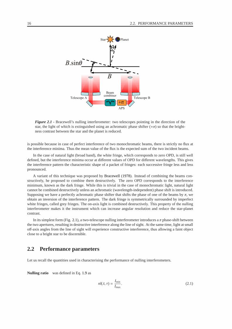
Figure 2.1 - Bracewell’s nulling interferometer: two telescopes pointing in the direction of thestar, the light of which is extinguished using an achromaticphase shifter (+π) so that the bright-ness contrast between the star and the planet is reduced.
is possible because in case of perfect interference of two monochromatic beams, there is strictly no flux atthe interference minima. Thus the mean value of the flux is theexpected sum of the two incident beams.
In the case of natural light (broad band), the white fringe, which corresponds to zero OPD, is still welldefined, but the interference minima occur at different values of OPD for different wavelengths. This givesthe interference pattern the characteristic shape of a packet of fringes: each successive fringe less and lesspronounced.
A variant of this technique was proposed byBracewell(1978). Instead of combining the beams con-structively, he proposed to combine them destructively. The zero OPD corresponds to the interferenceminimum, known as the dark fringe. While this is trivial in thecase of monochromatic light, natural lightcannot be combined destructively unless an achromatic (wavelength-independent) phase shift is introduced.Supposing we have a perfectly achromatic phase shifter thatshifts the phase of one of the beams byπ, weobtain an inversion of the interference pattern. The dark fringe is symmetrically surrounded by imperfectwhite fringes, called grey fringes. The on-axis light is combined destructively. This property of the nullinginterferometer makes it the instrument which can increase angular resolution and reduce the star-planetcontrast.
In its simplest form (Fig.2.1), a two-telescope nulling interferometer introduces aπ phase-shift betweenthe two apertures, resulting in destructive interference along the line of sight. At the same time, light at smalloff-axis angles from the line of sight will experience constructive interference, thus allowing a faint objectclose to a bright star to be discernible.
2.2 Performance parameters
Let us recall the quantities used in characterising the performance of nulling interferometers.
Nulling ratio was defined in Eq.1.9as
nl(λ, τ) =Imin
Imax. (2.1)

CHAPTER 2. NULLING INTERFEROMETRY 17
Rejection ratio is the inverse of the nulling ratio:
ρ(λ, τ) =Imax
Imin. (2.2)
Spectral band where the instrument operates is an inherent part of performance specifications. Both itsabsolute position in the electromagnetic spectrum and its width are important. The width is often expressedas a fraction (in per cent)
∆λ
λ. (2.3)
Stability is a measure of how longer exposure times reduce star-planetcontrast. For a set of values ofnl, calculate the moving (or running) average with a window of the durationτ. Take this set of movingaverages〈nl〉τ, each averaged over exposure timeτ, and calculate its standard deviationσ〈nl〉(τ). Now,repeat the procedure for a number of different windows widthsτ, and inspect the dependence ofσ〈nl〉(τ)uponτ. If it is consistent withτ−1/2 (i.e., white noise behaviour) up to a certainτmax, then
σ〈nl〉(τ = τmax) (2.4)
is a good expression of the nuller’s stability.
Rudiments of interferometry. In the simplest, monochromatic case, we can represent a single wave withan amplitude ofA as a function of the phaseφ:
S1 = A1eiφ1, (2.5)
and the corresponding intensityI1 is:I1 = |A1|2. (2.6)
Let us make two such waves interfere. The resulting complex sum is:
S = S1 + S2 = A1eiφ1 + A2eiφ2, (2.7)
and the intensityI isI = |A1|2 + |A2|2 + 2|A1||A2| cos(φ1 − φ2), (2.8)
which can be expessed as
I = I1 + I2 + 2√
I1I2 cos(φ1 − φ2). (2.9)
If I1 = I2, the interference pattern’s maximum,Imax, corresponds to|φ1 − φ2| = 0, i.e.,
Imax = 2I1 + 2I1 cos(0)= 4I1, (2.10)
whereas the minimum,Imin, corresponds to|φ1 − φ2| = π, i.e.,
Imin = 2I1 + 2I1 cos(π) = 0, (2.11)
hence the nulling ratio is
nl =Imin
Imax= 0. (2.12)
Let us examine the behaviour of the nulling ratio close to this value, i.e., for|φ1 − φ2| = ∆φ ≪ 1. In thiscase we obtain
nl =Imin
Imax=
1+ cos(π + ∆φ)1+ cos(∆φ)
=1− cos(∆φ)1+ cos(∆ϕ)
(2.13)

18 2.3. ACHROMATIC PHASE SHIFTERS
nl ≈1− 1+ ∆φ
2
2
1+ 1− ∆φ2
2
≈ ∆φ2
4for ∆φ ≪ 1. (2.14)
Let us now return to the situation where|φ1 − φ2| = 0, and examine what happens ifI1 , I2. Supposing
I2 = (1+ ǫ)I1, (2.15)
whereǫ ≪ 1. This means that the relative flux flux mismatch∆I/I is
∆II=
I2 − I1
I1=
(1+ ǫ)I1 − I1
I1=ǫ I1
I1= ǫ. (2.16)
The nulling rationl then is
nl =Imin
Imax=
I1 + I2 + 2√
I1I2 cos(π)
I1 + I2 + 2√
I1I2 cos(0)=
I1 + I2 − 2√
I1I2
I1 + I2 + 2√
I1I2, (2.17)
nl =I1 + (1+ ǫ)I1 − 2I1
√1+ ǫ
I1 + (1+ ǫ)I1 + 2I1
√1+ ǫ
=2+ ǫ − 2
√1+ ǫ
2+ ǫ + 2√
1+ ǫ, (2.18)
developing√
1+ ǫ:√
1+ ǫ = 1+ǫ
2− ǫ
2
8+ ... (2.19)
nl ≈2+ ǫ − 2(1+ ǫ2 −
ǫ2
8 )
2+ ǫ + 2(1+ ǫ2 −ǫ2
8 )=
−2−ǫ2
8
4+ 2ǫ + 2−ǫ2
8
, (2.20)
nl ≈ǫ2
16. (2.21)
2.3 Achromatic Phase Shifters
One of the key components of the Bracewell interferometer isthe Achromatic Phase Shifter (APS). It is anoptical element designed to introduce a given difference in phase in a beam regardless of the wavelength.
Let us state clearly that in real life there are no perfect optical elements that would fulfil this functionideally. There are many workable solutions, however, always representing a compromise between the“neatness” of the phase shift (how well does the real phase shift correspond to the required value), and thewidth of the spectral band in which it is to be achieved.
For a given Optical-Path Difference (OPD) between the two optical paths, the corresponding phasedifference∆ϕ can be expressed as
∆ϕ = 2πOPDλ, (2.22)
whereλ is the wavelength.
The phase shift therefore depends on the wavelength,∆ϕ = ∆ϕ(λ). In order to obtain a wavelength-independent phase shift ofπ at zero OPD, an APS has to be introduced into the setup.
There are alternative approaches, however. The “adaptive nuller” was tested at the JPL (Peters et al.2008), and at Delft, polarisation and multi-axial nulling interferometry were studied (Spronck et al. 2006).
Many different concepts of achromatic phase shifters are available in the literature (Rabbia et al. 2001,2000). TheDarwin collaboration studied ten APS concepts (ESA 2002), promisingnl < 10−6. The spectralrange was that of 6–20µm, with 6–18µm mandatory, the extension to 18–20µm priority number 2, andthat to 4–6µm priority number 3. Their various merits will eventually need to be evaluated experimentally.Not all of these concepts are currently in the research and development process. Some, although promising

CHAPTER 2. NULLING INTERFEROMETRY 19
(a) Dielectric or Dispersive Prisms (b) Field Reversal or Periscope
(c) Focus Crossing or Through Focus (d) Fresnel’s Rhombs
Figure 2.2 - The four APS concepts investigated by ESA.
in the long run, require a substantial effort to overcome technical hurdles chiefly because of the novelty andof the required spectral range (e.g., integrated optics, zero order gratings).
Out of the ten, four APS concepts were selected for further study by ESA in recent years (Fig.2.2):
1. Dielectric or Dispersive Prisms,
2. Focus Crossing or Through Focus,
3. Field Reversal or Periscope, and
4. Fresnel’s Rhombs.
The S testbed uses two pairs of CaF2 Prisms (Sec.3.11) as a Dispersive Prisms APS and, atthe same time, the prisms form an intrinsic part of the setup because they also function as a compensatorbalancing the cumulative thickness of dielectric in the optical path.
A Dispersive Prisms APS prototype with three pairs of prismsof three different materials was developedby Thales Alenia Space (Sec.3.9.3). A Focus Crossing APS prototype was designed by the Observatoirede Cote d’Azur, Nice, France (Sec.3.9.1). And, last but not least, a Field Reversal APS prototype wasmanufactured at Max-Planck-Institut fur Astronomie in Heidelberg in collaboration with Kayser-ThredeGmbH in Munich and the IOF Fraunhofer Institute for Applied Optics in Jena (Sec.3.9.2).

20 2.4. THE DISPERSIVE PRISMS APS
2.4 The Dispersive Prisms APS
Let us now look in more detail at the Dispersive Prisms APS because it of its role in the S setup. Thismethod is directly inspired by the practice of opticians whotry to minimise chromatic aberrations in lenssystems.
We shall examine one of the simplest cases when a pair of dispersive prisms is introduced into each armof the interferometer. The beams thus propagate in two different media, viz., in air and in the dielectric.The refractive indexndiel of the dielectric varies with wavelength,
ndiel = ndiel(λ). (2.23)
We shall consider air as not dispersive, i.e., its indexnair does not vary with wavelength
nair(λ) = 1. (2.24)
Because of the presence of the dispersive elements, the phase difference∆φ between the two beams willvary with wavelength
∆φ = ∆φ(λ). (2.25)
It can be expressed as
∆φ(λ) =2πλ
[nair · (OPD+ e) − e · ndiel(λ)] , (2.26)
wheree is the difference in thickness of dielectric encountered by the beams.Note that we can consider thetotal geometric length of the optical path constant, i.e., adding dielectric into the optical path reduces theair column in it by the same amount. We can thus write
∆φ(λ) =2πλ
[OPD· nair + e · (nair − ndiel(λ))] . (2.27)
Now we can impose∆φ(λ1) = π, (2.28)
∆φ(λ2) = π, (2.29)
for two distinct wavelengthsλ1,2. This is a set of two equations with two unknowns,eand OPD,
2πλ1
[OPD· nair + e · (nair − ndiel(λ1))] = π, (2.30)
2πλ2
[OPD· nair + e · (nair − ndiel(λ2))] = π. (2.31)
For given two wavelengths there are values ofe and OPD which correspond to a perfectnl = 0. If thematerial and the waveband are chosen appropriately, a Dispersive Prisms APS can provide nulling betterthan a specified value within the waveband (Fig.2.3).
Let us look at the dual problem: How do we find the working pointif we have the means to explorethe parameter space (OPD,e)? Fig. 2.4 shows that there are many local minima, and thus we need tounderstand this space better in order to find the global minimum. Performing an OPD scan for a given valueof e will yield a fringe packet. If the fringe packet is symmetric, we find a minimum (Fig.2.5). It could bea local minimum, however. The ambiguity can be lifted by looking at neighbouring minima. Section6.1.5describes a practical application of this technique.
2.5 Wavefront filtering
Another important ingredient in nulling interferometry iswavefront filtering. Achieving high levels ofdestructive interference implies stringent requirementsin terms of wavefront quality. These requirementscan be reduced using a wavefront filter (Mennesson et al. 2002).
There are two techniques of wavefront filtering used in nulling interferometry:

CHAPTER 2. NULLING INTERFEROMETRY 21
Figure 2.3 - Nulling ratio as a function of wavelength (inµm) produced by Dispersive PrismsAPS with two thicknesses of CaF2, one per beam. Appropriate selection of thicknesses ensuresthat in a given spectral band (highlighted) the nulling ratio is nl < 10−4. This is possible becauseCaF2 is dispersive, i.e., its refractive index varies with wavelength.
Figure 2.4 - Map of the (OPD,e) space. There are many local minima in the (OPD,e) parameterspace. Nonetheless, the global minimum is unique.

22 2.6. STABILITY
Figure 2.5 - Three OPD scans for different values ofe. Performing an OPD scan for a given valueof e will yield a fringe packet. If the fringe packet is symmetric, we find a minimum. It could bea local minimum, however. The ambiguity can be lifted by looking at neighbouring minima.
1. Pinholes, i.e., spatial filters;
2. Single-Mode optical Fibres (SMF’s), i.e., modal filters.
A SMF is, effectively, a waveguide that transmits only one resonance mode. We can view the fibreas a resonance cavity with a single resonance mode in the given spectral band. This resonance mode is asolution of Maxwell’s equations and is not confined to the internal volume of the fibre. In fact, it extendsfrom both extremities of the fibre as lobes. Therefore, whatever the properties of the optical field incidentupon the fibre head, the output of the fibre will be an extensionof this proper mode.
Nulling interferometers require that the wavefront be without distortion to a level ofλ/1000 if thenulling rationl is to be less than 10−5 (Sec.3.3.6). The reason is easily seen when we realise that if thereare defects in the wavefront, a part of the flux arrives at the point of interference out of phase. Withoutwavefront filtering, theλ/1000 requirement would be prohibitively strict because it implies that all theoptical surfaces must be polished to that level of precision.
Unfortunately, the only way to estimate the quality of SMF’sis to measure it with a specialised nullinginterferometer (Ksendzov et al. 2007).
2.6 Stability
Experimental studies of nulling interferometer testbeds (Serabyn 2003; Schmidtlin et al. 2005; Ollivier et al.2001; Vink et al. 2003; Alcatel; Brachet 2005) show that even in simple setups, the interference pattern isunstable, drifting with time. Even interferometers breadboarded on an optical bench in the relatively well-controlled laboratory environment (a priori simpler than the actualDarwin/TPF-I, with its multiple tele-scopes rotating in space) display drifts.Chazelas et al.(2006) give a quantitative summary of these effects,using data fromOllivier (1999); Alcatel; Vink et al. (2003).
We shall discuss this issue in detail in Chapter4.

CHAPTER 2. NULLING INTERFEROMETRY 23
2.7 State of the art
Since 1999, several groups performed a number of experimental studies of nulling interferometry in thelaboratory and on ground-based telescopes. In our bibliographical study we have drawn upon the summarytable prepared byChazelas(2007) and on Peter R. Lawson’s null-vs-bandwidth plot (Lawson 2009). Ourown updates are presented in Tab.2.1and Fig.2.6.
Nulling interferometry is a new and challenging field of optics. By its very nature it is probably themost sensitive, and hence the most delicate, of optical experiments. This means that phenomena which areof the second or third order, and therefore rarely taken intoconsideration in optics, can stand out in nullinginterferometry. It is a challenge, but it also is an opportunity to study them.
To summarise the current state of art in terms of demonstrating the feasibility ofDarwin/TPF-I, the bestprogress was made at the Jet Propulsion Laboratory. The Adaptive Nuller demonstrated thatnl = 10−5
can be achieved in broadband (34 %) around 10µm (Peters et al. 2008), and the Planet Detection Testbeddemonstrated 4-beam nulling withnl = 4× 10⁻⁶ and the detection of a simulated planet at a contrast levelof 2× 10⁶ (Martin et al. 2006).

24 2.7. STATE OF THE ART
0.0 0.1 0.2 0.3 0.4 0.5Bandwidth / central wavelength
10-7
10-6
10-5
10-4
10-3
10-2
Null D
epth
Bokhove 2003
Bokhove 2003
Bokhove 2003
Brachet 2005
Gabor 2008
Gabor 2008
Buisset 2006
Buisset 2006
Weber 2004
Morgan 2003
Vosteen 2005
Schmidtlin 2005
Schmidtlin 2005
Tavrov 2005
Flatscher 2003
Flatscher 2003
Ollivier 1999
Ollivier 1999
Martin 2003
Mennesson 2003
Mennesson 2003Wallace 2004
Mennesson 2006
Gappinger 2009
Gappinger 2009
Gappinger 2009
Gappinger 2009Gappinger 2009
Samuele 2007
Samuele 2007
Wallace 2000
Labadie 2007
Peters 2008
Visible
H band
K band
N band
Laboratory Nulling Results 1999-2009
0.00 0.01 0.02 0.03 0.04 0.05 0.06 0.07Bandwidth / central wavelength
10-6
10-5
Null D
epth
Bokhove 2003
Gabor 2008
Buisset 2006
Weber 2004
Martin 2003
Martin 2003
Wallace 2003
Schmidtlin 2005
Schmidtlin 2005
Flatscher 2003
Flatscher 2003
Martin 2003
Martin 2003
Martin 2005
Haguenauer 2006
Gappinger 2009
Gappinger 2009
Zoom on Laser Nulling Results
Figure 2.6 - Chart of nulling ratios achieved in laboratory experiments. The plot summarises thebest results reported in the indicated papers, plotting thenull depth against the bandwidth (givenas a fraction of the central wavelength). The unabridged bibliographical references are providedin Table2.1. Bottom plot provides a zoom on the narrow-band and laser experiment sector.

CHAPTER 2. NULLING INTERFEROMETRY 25
λcentral∆λλcentral
Null Pol Reference Experiment
600 nm 0.5 1× 10⁻³ – Tavrov et al.(2005) Tokyo632.8 nm 3× 10⁻⁶ 2× 10⁻⁴ – Bokhove et al.(2003) TNO TPD, Delft632.8 nm 3× 10⁻⁶ 2.9× 10⁻⁶ + Bokhove et al.(2003) TNO TPD, Delft632.8 nm 3× 10⁻⁶ 7.4× 10⁻⁷ + Martin et al.(2003b) Rot. Shear. Int., best632.8 nm 3× 10⁻⁶ 4× 10⁻⁶ + Martin et al.(2003b) Rot. Shear. Int., stab.632.8 nm 3× 10⁻⁶ 1.3× 10⁻⁶ – Haguenauer and Serabyn(2006) Fiber Nuller, JPL635 nm 3× 10⁻⁶ 5.2× 10⁻⁶ + Wallace et al.(2003) Opt. Pl. Det. Int., JPL638 nm 3× 10⁻⁶ 1× 10⁻⁶ + Schmidtlin et al.(2005) Opt. Pl. Det. Int., JPL638 nm 3× 10⁻⁶ 1.11× 10⁻⁷ – Samuele et al.(2007) Northrop, Redondo B.650 nm 0.24 2× 10⁻³ – Bokhove et al.(2003) TNO TPD, Delft650 nm 0.24 1.1× 10⁻³ + Bokhove et al.(2003) TNO TPD, Delft650 nm 0.3 2.1× 10⁻⁴ – Vosteen et al.(2005) Delft; Friedrichshafen650 nm 0.05 8.3× 10⁻⁶ + Schmidtlin et al.(2005) Opt. Pl. Det. Int., JPL650 nm 0.12 3.2× 10⁻⁵ + Schmidtlin et al.(2005) Opt. Pl. Det. Int., JPL650 nm 0.15 1× 10⁻⁶ – Samuele et al.(2007) Northrop, Redondo B.650 nm 0.18 7.1× 10⁻⁵ + Wallace et al.(2000) JPL700 nm 0.28 7× 10⁻³ – Morgan et al.(2003) Nulling B. Comb., JPL1306 nm 8× 10⁻⁵ 2.5× 10⁻⁶ – Flatscher et al.(2003) Astrium, Friedrichshafen1.54µm 3× 10⁻⁶ 1.3× 10⁻⁶ + Weber(2004) MAII I, Cannes1.545µm 0.02 3.1× 10⁻⁵ – Flatscher et al.(2003) Astrium, Friedrichshafen1.55µm 0.05 2.7× 10⁻⁵ – Buisset et al.(2007) MAII II, Cannes1.55µm 0.05 6× 10⁻⁶ + Buisset et al.(2007) MAII II, Cannes1.55µm 1× 10⁻³ 4.3× 10⁻⁶ – Flatscher et al.(2003) Astrium, Friedrichshafen1.57µm 0.05 1.7× 10⁻⁴ – Weber(2004) MAII I, Cannes1.65µm 0.18 5× 10⁻⁴ – Mennesson et al.(2006) Fiber Nuller, JPL2.2µm 0.18 2.5× 10⁻⁴ – Brachet(2005) S I; IAS Orsay3.39µm 3× 10⁻⁶ 1× 10⁻⁵ + Gabor et al.(2008c) S II; IAS Orsay3.39µm 3× 10⁻⁶ 1× 10⁻⁴ – Gabor et al.(2008c) S II; IAS Orsay9.5µm 0.2 2× 10⁻⁵ + Gappinger et al.(2009) Achr. Nulling T., perisc.9.5µm 0.25 4× 10⁻⁵ + Gappinger et al.(2009) Achr. Nulling T., perisc.9.5µm 0.25 6.7× 10⁻⁴ – Gappinger et al.(2009) Achr. Nulling T., FC9.5µm 0.30 9.1× 10⁻⁵ – Gappinger et al.(2009) Achr. Nulling T., 2Prism9.5µm 0.30 8.8× 10⁻⁵ – Gappinger et al.(2009) Achr. Nulling T., 1Prism10µm 0.30 1× 10⁻⁴ – Wallace et al.(2004) Warm Nulling Testbed, JPL10µm 3× 10⁻⁶ 3.3× 10⁻⁶ + Gappinger et al.(2009) Achr. Nulling T., perisc.10µm 3× 10⁻⁶ 1.1× 10⁻⁵ – Gappinger et al.(2009) Achr. Nulling T., perisc.10µm 0.4 1× 10⁻⁵ + Peters et al.(2008) Adaptive Nuller T., JPL
10.6µm 3× 10⁻⁶ 1× 10⁻³ – Ollivier (1999) IAS Orsay; typ.10.6µm 3× 10⁻⁶ 7× 10⁻⁴ – Ollivier (1999) IAS Orsay; best10.6µm 3× 10⁻⁶ 1.1× 10⁻⁶ – Martin et al.(2003a) MMZ Nuller, JPL10.6µm 3× 10⁻⁶ 7× 10⁻⁷ + Martin et al.(2003a) MMZ Nuller, JPL10.6µm 3× 10⁻⁶ 7.3× 10⁻⁶ – Martin et al.(2005) Planet Detection T., JPL10.6µm 3× 10⁻⁶ 5.6× 10⁻⁵ – Labadie et al.(2007) Grenoble
10.675µm 0.18 5.9× 10⁻⁵ – Mennesson et al.(2003) Keck Nuller B. Comb., JPL10.775µm 0.29 1.3× 10⁻⁴ – Mennesson et al.(2003) Keck Nuller B. Comb., JPL
Table 2.1 - Main nulling-interferometry laboratory results, orderedaccording to spectral band(first column). The second column gives the bandwidth (as a fraction of the central wavelength),the third column give the best null achieved, the “Pol” column indicates whether polarisers wereused at the output. The “Reference” and “Experiment” columns indicate the setup (“Achr. NullingT.” is the Achromatic Nulling Testbed at the JPL which had several phase shifter options: “perisc.”was the periscope, “FC” was the through focus or focus crossing, “1Prism” was a setup with ZnSedispersive prisms, “2Prism” was a setup with ZnSe and ZnS prisms).

26 2.7. STATE OF THE ART

Chapter 3Description of S & N
Contents3.1 Introduction . . . . . . . . . . . . . . . . . . . . . . . . . . . . . . . . . . . . . . . . . 28
3.1.1 The purpose of this Chapter. . . . . . . . . . . . . . . . . . . . . . . . . . . . . 28
3.1.2 General note. . . . . . . . . . . . . . . . . . . . . . . . . . . . . . . . . . . . . 28
3.1.3 Historical background. . . . . . . . . . . . . . . . . . . . . . . . . . . . . . . . 29
3.2 General overview . . . . . . . . . . . . . . . . . . . . . . . . . . . . . . . . . . . . . . 323.2.1 An outline. . . . . . . . . . . . . . . . . . . . . . . . . . . . . . . . . . . . . . . 32
3.2.2 General layout. . . . . . . . . . . . . . . . . . . . . . . . . . . . . . . . . . . . 33
3.3 Purpose of the subsystems. . . . . . . . . . . . . . . . . . . . . . . . . . . . . . . . . . 363.3.1 A point source observed by two apertures. . . . . . . . . . . . . . . . . . . . . . 36
3.3.2 Three remarks on single-mode fibres. . . . . . . . . . . . . . . . . . . . . . . . . 36
3.3.3 Off-axis parabolic mirrors . . . . . . . . . . . . . . . . . . . . . . . . . . . . . . 37
3.3.4 Symmetry. . . . . . . . . . . . . . . . . . . . . . . . . . . . . . . . . . . . . . . 38
3.3.5 Flux balancing. . . . . . . . . . . . . . . . . . . . . . . . . . . . . . . . . . . . 40
3.3.6 Stability. . . . . . . . . . . . . . . . . . . . . . . . . . . . . . . . . . . . . . . . 41
3.3.7 Optical path. . . . . . . . . . . . . . . . . . . . . . . . . . . . . . . . . . . . . . 43
3.4 Sources . . . . . . . . . . . . . . . . . . . . . . . . . . . . . . . . . . . . . . . . . . . . 443.4.1 Ceramic black body. . . . . . . . . . . . . . . . . . . . . . . . . . . . . . . . . 44
3.4.2 3.39µm HeNe laser . . . . . . . . . . . . . . . . . . . . . . . . . . . . . . . . . 46
3.4.3 Supercontinuum laser source. . . . . . . . . . . . . . . . . . . . . . . . . . . . . 46
3.4.4 2.32µm laser diode. . . . . . . . . . . . . . . . . . . . . . . . . . . . . . . . . . 47
3.5 Modal filters . . . . . . . . . . . . . . . . . . . . . . . . . . . . . . . . . . . . . . . . . 483.5.1 Fluoride-Glass Single-Mode Fibres. . . . . . . . . . . . . . . . . . . . . . . . . 48
3.5.2 Fibre output aperturing. . . . . . . . . . . . . . . . . . . . . . . . . . . . . . . . 48
3.6 Spectral filters . . . . . . . . . . . . . . . . . . . . . . . . . . . . . . . . . . . . . . . . 483.7 Polarisers . . . . . . . . . . . . . . . . . . . . . . . . . . . . . . . . . . . . . . . . . . . 503.8 Detectors . . . . . . . . . . . . . . . . . . . . . . . . . . . . . . . . . . . . . . . . . . . 50
3.8.1 Array detector . . . . . . . . . . . . . . . . . . . . . . . . . . . . . . . . . . . . 50
3.8.2 Single element detector. . . . . . . . . . . . . . . . . . . . . . . . . . . . . . . . 50
3.9 Phase shifter prototypes. . . . . . . . . . . . . . . . . . . . . . . . . . . . . . . . . . . 533.9.1 Focus Crossing or Through Focus. . . . . . . . . . . . . . . . . . . . . . . . . . 53
3.9.2 Field Reversal or Periscope. . . . . . . . . . . . . . . . . . . . . . . . . . . . . . 53
3.9.3 Dispersive prisms. . . . . . . . . . . . . . . . . . . . . . . . . . . . . . . . . . . 54
3.10 Electronics & Software . . . . . . . . . . . . . . . . . . . . . . . . . . . . . . . . . . . 54

28 3.1. INTRODUCTION
3.10.1 Lock-in amplifier. . . . . . . . . . . . . . . . . . . . . . . . . . . . . . . . . . . 55
3.10.2 Software. . . . . . . . . . . . . . . . . . . . . . . . . . . . . . . . . . . . . . . 56
3.11 S . . . . . . . . . . . . . . . . . . . . . . . . . . . . . . . . . . . . . . . . . . . . 603.12 S II . . . . . . . . . . . . . . . . . . . . . . . . . . . . . . . . . . . . . . . . . . . 633.13 N . . . . . . . . . . . . . . . . . . . . . . . . . . . . . . . . . . . . . . . . . . 64
3.1 Introduction
3.1.1 The purpose of this Chapter
The purpose of this Chapter is to provide a detailed description of the two nulling testbeds currently op-erating at theInstitut d’Astrophysique Spatialein Orsay, France, namely the S and the Ninstruments.
N can be regarded as the successor of S: the know-how and insights we acquired whileworking on S went into the design of N. This thesis is primarily a report on S.Nonetheless, since N inherited many subsystems from S (certain light sources, detectors,single-mode fibres, etc.), it will not be too difficult to describe both testbeds.
What is more, our ambition is to provide an instructive text that future generations of students workingwith these testbeds would find useful. We shall, therefore, devote considerable space to the reasoning behindthe design choices: and we hope that a parallel description of both testbeds will help us to achieve this goal.
3.1.2 General note
It must be noted that the two experiments are still a going concern. Their full potential has not been reachedso far. If there were enough manpower, both experimental setups could be studied in parallel. We shall seethat S is a more elegant optical design than N which is more straightforward but also morerobust. Certain aspects of S still need to be explained fully, and N was designed to help inthis regard. However, once a better understanding is reached with N, it could be very satisfying togo back to S in order to verify the theory.
The fact that the experiments are ongoing does not merely mean that some set of goals has not beenreached so far, but also that the objectives themselves are still evolving: not knowing the full potential of thetestbeds, the work itself gradually brings forth the possible objectives to be reached. I am stressing this pointbecause in the logical order of things the reader might expect that a description of an experiment shouldstart with an account of its purpose. Should it not be the purpose that dictates the operational parametersand therefore the choice of means to achieve them? Should thework not have evolved linearly according toa predetermined plan, such as the one outlined below?
• Objective: compare the achromatic phase shifter performance in the K band.
• Since the theoretical limits of the phase shifter prototypes are to be expected at the null levels ofnl = 10−5, the testbed must reach at leastnl = 3× 10⁻⁶.
• In order to reach such null levels, and in view of other constraints (flux levels of available sources,quality and performance of optical elements including modal filters, precision of alignment proce-dures, sensitivity of available detectors, etc.) the setuphas to have such and such an optical design.
Although there have certainly been elements of such linear planning present during the development ofthe testbeds in Orsay, neither S nor N can be fully understood in such a framework. As withall pioneering projects, the testbeds can only be fully understood and appreciated as vehicles of discovery.Their ultimate purpose is not to reach certain predefined performance levels butto learn in detail aboutphenomena hitherto known only by extrapolation.

CHAPTER 3. DESCRIPTION OF SYNAPSE & NULLTIMATE 29
Figure 3.1 - A global view of the first nulling testbed at theInstitut d’Astrophysique Spatiale(Ollivier 1999). It operated at ambient temperature in monochromatic polarised light at 10.6µmand achievednl = 7× 10⁻⁴.
This is fundamentally the reason why this Chapter does not follow the classical, linear plan which woulddefine the layout as a solution to the problem of reaching the objectives with available means. The choiceswere, naturally, dictated by considerations aimed at optimising performance. However, the process was notlinear, and this Chapter would not benefit from attempts to follow the rationale behind each experimentalchoice. We shall, therefore, limit ourselves to a simple description of the equipment.
3.1.3 Historical background
3.1.3.1 Monochromatic10.6µm testbed
The Institut d’Astrophysique Spatialein Orsay, France, has been involved in nulling interferometry since1995 when Marc Ollivier started his thesis under Alain Leger’s direction (Ollivier et al. 2001; Ollivier1999). His testbed (Fig.3.1) operated at ambient temperature in monochromatic polarised light at 10.6µmand achievednl = 7× 10⁻⁴.
3.1.3.2 TheS testbed
The second effort was the S1 testbed (Fig.3.2), again designed for operation at ambient temperature,but in polychromatic light in the K band, i.e., between 2.0–2.5µm (Brachet 2005). The primary aim of this
1SYmmetric Nuller for Achromatic Phase Shifter Evaluation

30 3.1. INTRODUCTION
Figure 3.2 - A view of the S nulling testbed’s interferometric setup (Brachet 2005, photo-graph taken in Sept. 2003).
apparatus was achromatic phase shifter testing. This purpose drove the optical design towards symmetry.
3.1.3.3 TheS II testbed
It soon became apparent that stability is a crucial issue in nulling interferometry, and an upgraded versionof the S testbed was implemented. It is known as S II (Gabor et al. 2008c).
3.1.3.4 TheN testbed
In parallel with S II, the team planned a new setup at 10.6µm, this time in cryogenic conditions(Chazelas 2007). The project was called N2. Considerable effort was dedicated to the cryogenicdesign (3.3) but in the end it was decided to postpone its realisation until the experimental technique is fullymastered at ambient temperature in the K band. This is why theN testbed was finally designedfor operational parameters very much like those of S but with a different optical design (Fig.3.4).
3.1.3.5 TheP testbed
The IAS team is currently also involved in the P3 testbed (Fig.3.5) which was designed as a demon-strator for the P mission proposal (Principal Investigator: Marc Ollivier). P is currently beinginstalled at the Observatory of Paris in Meudon. The design and tests of several subsystems took place atIAS, however. The scope of our report must be limited, and we shall concentrate on two testbeds: Sand N.
2NULling Low Temperature Interferometer for Multi Achromatic phase shifter TEsting3P Experiment for Research and Stabilization of Extreme Extinctions

CHAPTER 3. DESCRIPTION OF SYNAPSE & NULLTIMATE 31
Figure 3.3 - The N testbed was originally designed for cryogenic conditions (10−4 torr,100 K) andλ ≈ 10µm (Chazelas 2007).
Figure 3.4 - General view of N (during alignment).

32 3.2. GENERAL OVERVIEW
Figure 3.5 - A view of the P testbed.
3.2 General overview
3.2.1 An outline
The experimental setup contains the main optical chain of subsystems (the sources, the interferometerproper, the detectors), as well as a number of auxiliary subsystems (alignment instruments, experimentcontrol electronics and software, data acquisition hardware and software, antivibration protection, thermaland accoustic insulation, temperature control). All of these will be described in detail after we first providean outline of the whole.
The general purpose of both setups, S and N, is to achieve high levels of stable nullingperformance first in the K band (for our purposes defined asλ ∈ [2.0,2.5]µm), and eventually atλ = 10µm.This means we need two identical beams, corresponding to thetelescope apertures following the samefield of view on the sky, we need to combine them interferometrically, and we need to detect the result.Both testbeds create the two identical beams by splitting a single beam into two. Combining the beamsinterferometrically means that the optical path of both beams must be of equal length. We therefore needto include delay lines and dielectric compensating plates or wedges to equate the optical paths of the twobeams. Furthermore, polychromatic nulling requires that aphase shift ofπ be introduced between the twobeams achromatically. And finally, when combined, the beamsmust be of equal flux and the wavefrontsmust be of adequate quality. An additional optical subsystem, namely two polarisers, one at each end ofthe interferometer, proved invaluable not only in providing additional information but in improving theperformance.
The minimal list of optical subsystems can be outlined as follows:
• Source, generating a single beam.
• Beam splitting subsystem creating two identical beams.
• Delay lines and dielectric compensators.

CHAPTER 3. DESCRIPTION OF SYNAPSE & NULLTIMATE 33
• Achromatic phase shifters.
• Flux balance control.
• Wavefront filter.
• Polarisers.
• Beam combining subsystem.
• Detector subsystem.
There is also a number of auxiliary systems that need to be described:
• Alignment instruments.
• Temperature control.
• Antivibration protection.
• Thermal and accoustic insulation.
• Experiment control hardware and software.
• Data acquisition hardware and software.
Experiments are not fully determined by the instruments andtheir layout: the operational methodologyis a crucial part of the whole process of experimental work. We shall, therefore, devote a part of this Chapteralso to an outline of certain procedures, techniques and protocols, leaving a detailed discussion of some ofthem to the following Chapters (4 and5).
3.2.2 General layout
Let us start with a general view of each of our two testbeds.
3.2.2.1 S
Whereas the interferometer proper is installed on a dedicated optical table, the sources as well as the detec-tors reside on their own optical benches, mechanically decoupled from the interferometer’s primary bench(Fig. 3.6). These three tables are optically linked with optical fibres. Since we use single-mode fibres, thefibre linking the interferometer with the detector also serves as a modal filter. The interferometer with itsdedicated optical table is insulated by a plexiglass enclosure with an optional imposed inverse heat gradient(Fig. 3.7).
3.2.2.2 N
Fig. 3.8shows the N testbed with its protective casing. Here, the sources and the detectors are allinstalled on the same optical table as the interferometer proper. The interferometer is encased in a plexiglassenclosure, mechanically decoupled from the optical table.Again, single-mode optical fibres are used but,unlike in the case of S, they are not necessary to provide an optical link between the sources, theinterferometer proper and the detector since these opticalsubsystems are all installed on the same opticaltable. Like in S, the purpose of the single-mode fibre linking the interferometer and the detector ismodal filtering of the wavefront. The purpose of the fibre linking the sources with the interferometer properis less crucial, however. It merely provides the same beam geometry regardless of which source is beingused.

34 3.2. GENERAL OVERVIEW
Figure 3.6 - S experimental setup: The interferometer itself is mechanically decoupledfrom the source and detector systems. The whole setup is installed on a granit block supportedby six pneumatic legs (passive). Further, the interferometer’s optical table stands on three piezo-electric active legs (Brachet 2005).
Figure 3.7 - The interferometer table of S is enclosed in a plexiglass enclosure. Its top canbe heated in order to impose a thermal gradient to minimise air turbulence (Brachet 2005).

CHAPTER 3. DESCRIPTION OF SYNAPSE & NULLTIMATE 35
Figure 3.8 - N on its optical table, with protective casing.
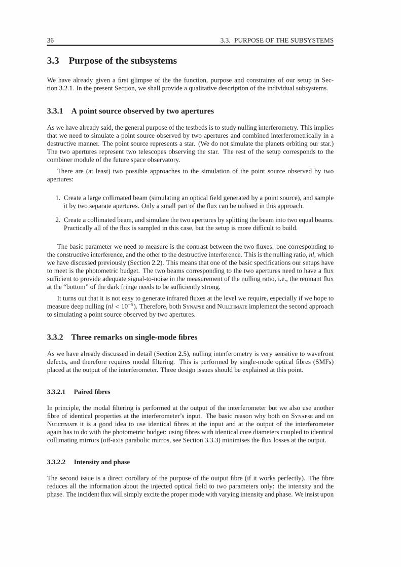
36 3.3. PURPOSE OF THE SUBSYSTEMS
3.3 Purpose of the subsystems
We have already given a first glimpse of the the function, purpose and constraints of our setup in Sec-tion 3.2.1. In the present Section, we shall provide a qualitative description of the individual subsystems.
3.3.1 A point source observed by two apertures
As we have already said, the general purpose of the testbeds is to study nulling interferometry. This impliesthat we need to simulate a point source observed by two apertures and combined interferometrically in adestructive manner. The point source represents a star. (Wedo not simulate the planets orbiting our star.)The two apertures represent two telescopes observing the star. The rest of the setup corresponds to thecombiner module of the future space observatory.
There are (at least) two possible approaches to the simulation of the point source observed by twoapertures:
1. Create a large collimated beam (simulating an optical field generated by a point source), and sampleit by two separate apertures. Only a small part of the flux can be utilised in this approach.
2. Create a collimated beam, and simulate the two apertures by splitting the beam into two equal beams.Practically all of the flux is sampled in this case, but the setup is more difficult to build.
The basic parameter we need to measure is the contrast between the two fluxes: one corresponding tothe constructive interference, and the other to the destructive interference. This is the nulling ratio,nl, whichwe have discussed previously (Section2.2). This means that one of the basic specifications our setups haveto meet is the photometric budget. The two beams corresponding to the two apertures need to have a fluxsufficient to provide adequate signal-to-noise in the measurement of the nulling ratio, i.e., the remnant fluxat the “bottom” of the dark fringe needs to be sufficiently strong.
It turns out that it is not easy to generate infrared fluxes at the level we require, especially if we hope tomeasure deep nulling (nl < 10−5). Therefore, both S and N implement the second approachto simulating a point source observed by two apertures.
3.3.2 Three remarks on single-mode fibres
As we have already discussed in detail (Section2.5), nulling interferometry is very sensitive to wavefrontdefects, and therefore requires modal filtering. This is performed by single-mode optical fibres (SMFs)placed at the output of the interferometer. Three design issues should be explained at this point.
3.3.2.1 Paired fibres
In principle, the modal filtering is performed at the output of the interferometer but we also use anotherfibre of identical properties at the interferometer’s input. The basic reason why both on S and onN it is a good idea to use identical fibres at the input and at the output of the interferometeragain has to do with the photometric budget: using fibres withidentical core diameters coupled to identicalcollimating mirrors (off-axis parabolic mirros, see Section3.3.3) minimises the flux losses at the output.
3.3.2.2 Intensity and phase
The second issue is a direct corollary of the purpose of the output fibre (if it works perfectly). The fibrereduces all the information about the injected optical fieldto two parameters only: the intensity and thephase. The incident flux will simply excite the proper mode with varying intensity and phase. We insist upon
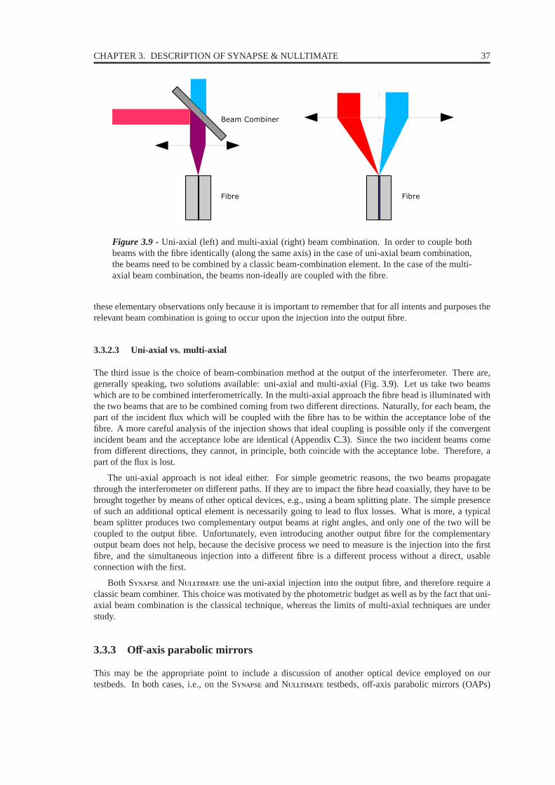
CHAPTER 3. DESCRIPTION OF SYNAPSE & NULLTIMATE 37
Figure 3.9 - Uni-axial (left) and multi-axial (right) beam combination. In order to couple bothbeams with the fibre identically (along the same axis) in the case of uni-axial beam combination,the beams need to be combined by a classic beam-combination element. In the case of the multi-axial beam combination, the beams non-ideally are coupled with the fibre.
these elementary observations only because it is importantto remember that for all intents and purposes therelevant beam combination is going to occur upon the injection into the output fibre.
3.3.2.3 Uni-axial vs. multi-axial
The third issue is the choice of beam-combination method at the output of the interferometer. There are,generally speaking, two solutions available: uni-axial and multi-axial (Fig.3.9). Let us take two beamswhich are to be combined interferometrically. In the multi-axial approach the fibre head is illuminated withthe two beams that are to be combined coming from two different directions. Naturally, for each beam, thepart of the incident flux which will be coupled with the fibre has to be within the acceptance lobe of thefibre. A more careful analysis of the injection shows that ideal coupling is possible only if the convergentincident beam and the acceptance lobe are identical (Appendix C.3). Since the two incident beams comefrom different directions, they cannot, in principle, both coincidewith the acceptance lobe. Therefore, apart of the flux is lost.
The uni-axial approach is not ideal either. For simple geometric reasons, the two beams propagatethrough the interferometer on different paths. If they are to impact the fibre head coaxially, they have to bebrought together by means of other optical devices, e.g., using a beam splitting plate. The simple presenceof such an additional optical element is necessarily going to lead to flux losses. What is more, a typicalbeam splitter produces two complementary output beams at right angles, and only one of the two will becoupled to the output fibre. Unfortunately, even introducing another output fibre for the complementaryoutput beam does not help, because the decisive process we need to measure is the injection into the firstfibre, and the simultaneous injection into a different fibre is a different process without a direct, usableconnection with the first.
Both S and N use the uni-axial injection into the output fibre, and therefore require aclassic beam combiner. This choice was motivated by the photometric budget as well as by the fact that uni-axial beam combination is the classical technique, whereasthe limits of multi-axial techniques are understudy.
3.3.3 Off-axis parabolic mirrors
This may be the appropriate point to include a discussion of another optical device employed on ourtestbeds. In both cases, i.e., on the S and N testbeds, off-axis parabolic mirrors (OAPs)

38 3.3. PURPOSE OF THE SUBSYSTEMS
are used rather extensively.
1. Firstly, some of the sources effectively generate divergent beams, which then have to be collimatedwith OAPs. As we shall see in more detail in the next Section (3.4), this is the case of the ceramicblack body, of the supercontinuum laser source, as well as ofthe laser diode.
2. Then, the collimated beams have to be injected into single-mode optical fibres through which theyenter the beam-splitting setup used to generate the two beams ultimately destined to interfere at theend of the optical path. As we know, the testbeds simulate a star, the light of which they endeavour toeliminate interferometrically. The light beam produced atthe output of this single-mode optical fibresimulates our “star”.
3. At the output end of the star fibre, another OAP is used to generate a collimated beam, which thenenters the beam-splitting subsystem generating the two beams which will pass through the testbed.
4. At the end of the bench, after the beam combiner, the combined beam is injected into the outputsingle-mode optical fibre using another OAP.
5. And finally, at the output of the testbed’s output fibre the last OAP is used to collimate the light exitingthe fibre, and send it to the detector.
An OAP is (usually) an intersection of a paraboloid with a cylinder, their principal axes parallel. Theangle between the principal axis and the radiusr running from the paraboloid’s focus to the central point ofthe OAP, is its angleα (Fig. C.1). It is one of the characteristics of a given OAP. The length of this radiusris
r =2 f
1+ cosα. (3.1)
We provide description of Gaussian beams coupling to OAPs inAppendixC. Let us merely recall onenon-intuitive property. One might think that the OAP is likea funnel, “pouring” photons into the fibre. Sucha metaphor is misleading because, in fact, it implies that the whole of a “smaller” beam could be “poured”into a “larger” fibre. This is not the case. Fibre coupling is more like a resonance: the two optical fields arebest coupled when they are of identical shape.
3.3.4 Symmetry
As we have already seen in connection with the coupling efficiency (Section3.3.2.1, 3.3.3, C.3), symmetryof the design is one the key principles in our approach. In fact, the optical design of the S testbedcan be seen as an exercise in symmetry. The beam splitting subsystem is designed in order to produce twoidentical beams, and the beam combiner is the beam splitter’s exact counterpart.
In the case of the N testbed, it was decided that symmetry would take second place aftersimplicity. Nonetheless, interferometry is impossible without a certain measure of symmetry. N’stwo beams are not identical, but symmetry must be respected,and therefore the beam splitter is a mirrorimage of the beam combiner.
S implements a solution proposed bySerabyn and Colavita(2001) (Fig. 3.10, 3.11) which issymmetric by design. The dielectric plates need coatings sothat the system produces beams of equalintensity.
The beam-splitter plates are plane-parallel which means that stray light, due to multiple internal reflec-tions in the plate, has to be dealt with. The classic solution, which was implemented on N, is touse slightly prismatic plates. S, however, uses a different approach where the stray light is deflectedfrom contaminating the science beam’s path by the shape and proportions of the plates. N, withits classic solution, has to deal with beam dispersion on theprismatic beam splitter. An antisymmetricallyoriented identical optical element, acting as a compensator plate, is placed as close to the beam splitter aspossible.
In Section3.3.7we shall address the issue of balancing the thickness of dielectric in the two beams.

CHAPTER 3. DESCRIPTION OF SYNAPSE & NULLTIMATE 39
Figure 3.10 - Serabyn-Colavita modified Mach-Zehnder beam splitter.
Figure 3.11 - Serabyn-Colavita modified Mach-Zehnder beam combiner.
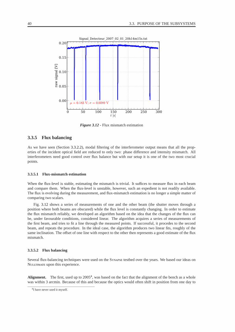
40 3.3. PURPOSE OF THE SUBSYSTEMS
0 50 100 150 200 250 300]s[t
0.00
0.05
0.10
0.15
0.20
raw
sig
nal
[V]
Signal_Detecteur_2007_02_01_20h14m15s.txt
V9820.0=σ;V381.0=µ
Figure 3.12 - Flux mismatch estimation
3.3.5 Flux balancing
As we have seen (Section3.3.2.2), modal filtering of the interferometer output means that all the prop-erties of the incident optical field are reduced to only two: phase difference and intensity mismatch. Allinterferometers need good control over flux balance but withour setup it is one of the two most crucialpoints.
3.3.5.1 Flux-mismatch estimation
When the flux-level is stable, estimating the mismatch is trivial. It suffices to measure flux in each beamand compare them. When the flux-level is unstable, however, such an expedient is not readily available.The flux is evolving during the measurement, and flux-mismatch estimation is no longer a simple matter ofcomparing two scalars.
Fig. 3.12 shows a series of measurements of one and the other beam (the shutter moves through aposition where both beams are obscured) while the flux level is constantly changing. In order to estimatethe flux mismatch reliably, we developed an algorithm based on the idea that the changes of the flux canbe, under favourable conditions, considered linear. The algorithm acquires a series of measurements ofthe first beam, and tries to fit a line through the measured points. If successful, it procedes to the secondbeam, and repeats the procedure. In the ideal case, the algorithm produces two linear fits, roughly of thesame inclination. The offset of one line with respect to the other then represents a good estimate of the fluxmismatch.
3.3.5.2 Flux balancing
Several flux-balancing techniques were used on the S testbed over the years. We based our ideas onN upon this experience.
Alignment. The first, used up to 20054, was based on the fact that the alignment of the bench as a wholewas within 3 arcmin. Because of this and because the optics would often shift in position from one day to
4I have never used it myself.

CHAPTER 3. DESCRIPTION OF SYNAPSE & NULLTIMATE 41
another, tuning the orientation of several mirrors before each experimental session was not only consideredacceptable: it was necessary. Flux optimisation and balancing was a natural part of the process.
Blades. With the improvement of alignment accuracy (within 10 arcsec), and especially after implement-ing the more solid mechanical design known as S II, it was no longer felt that touching the alignmentwas acceptable unless there was clear evidence of a shift in position. A dedicated flux-balancing device wastherefore designed. It was based on two blade-bearing translation stages, one operated by a manual screw,while the other by a motorised one (Newport’s “CMA-12PP” with a “SMC200” controller).
Injection into the output fibre. The coupling of each of the two beams with the output fibre is verysensitive to beam shear and tip-tilt. The relative situation of the beams is determined at the beam-combinerlevel. After that both beams encounter the same optical elements, viz., folding mirrors, the off-axis parabolaand the output fibre. Our alignment procedures ensure that atthe output of the beam combiner, the beamshear is
d ≈ 0.1 mm (3.2)
and the misalignment isδ ≈ 5 arcsec (3.3)
This means that if one beam is perfectly coupled with the fibre, the other necessarily is not. Finemovement of the folding mirrors can nonetheless always find aworking point where both beams are equallywell injected.
The procedure of flux balancing thus also fulfils the role of the last alignment procedure, compensatingfor the imperfection of beam superposition.
3.3.6 Stability
If it can be said that interference is the optical phenomenonwhich is the most sensitive to perturbationsof all sorts, it is even more true in the case of nulling interferometry. This means that one of the guidingprinciples in the design of our testbeds was their mechanical and thermal stability.
Let us illustrate this point in terms of the optical path difference. If the nulling performance is to bemaintained, e.g., below the level ofnl = 10−5, then (in the absence of other perturbations) the optical pathdifference must be maintained within
∆φ2
4< nl = 10−5 (3.4)
∆φ < 2√
nl = 6.3× 10⁻³ (3.5)
2πOPDλ< 2√
nl = 6.3× 10⁻³ (3.6)
OPD<λ√
nlπ= 10−3λ (3.7)
In the K band (λmin = 2.0µm), therefore,
OPD< 10−3λ = 2 nm (3.8)
Since we want to perform our nulling experiments in the K band, we need to make sure that we controlthe OPD to within nanometric levels. On such scaleseverythingmoves. We need to make sure, therefore,to make good use of all strategies available.

42 3.3. PURPOSE OF THE SUBSYSTEMS
Before we outline our choices for testbed stabilisation, let us stress a point we already mentioned above(Section3.1.2). Although the declared purposes of both S and N were tests of achromaticphase shifter prototypes, null stability, etc., the fundamental goal of these experiments is a better under-standing of all the issues involved in nulling interferometry. The level of accuracy and stability required fornulling is such that it is only prudent to make sure thatall potential perturbations are well known and undercontrol.
The constraint of OPD being withinλ/1000 is a formidable challenge in its own right. But our problemis much more daunting because it is perfectly clear that OPD control is by farnot the onlyissue we haveto deal with. In order to study all the perturbative effects, we need to be able to distinguish them, and thatmeans making very sure that we indeed do have OPD under control so that we can study the impact of otherparameters.
Let us now look at the available stabilisation techniques. They can be divided broadly into two cate-gories: passive and active. The passive ones are based on themechanical design of the optical table, themounts, and the casing. The active ones are those employing servo loops.
3.3.6.1 Ambient conditions
From the very first picture of S we have reproduced here (Fig.3.6), it is clear that one of the chiefconcerns in its design was the issue of ambient conditions.
• We havetemperatureandhumiditycontrol (of varying quality) in both rooms where S andN are installed.
• What is more, the interferometers are installed in protective cases to minimiseair turbulenceandreduce acoustic perturbations.
• The S testbed’s protective case has a heating system which can introduce a temperature gradi-ent in the volume of air, therebyreducing uncontrolled convection.
• The optical tables haveantivibrationfeatures and are mechanically isolated from the floor.
We shall discuss the relevance and efficiency of all these measures in due course (Section5.1.1).
3.3.6.2 Mechanics
The mounts of our optics likewise play a crucial role in the stability of the setup. The criteria to be con-sidered concern not only their rigidity but also their practicality during alignment procedures in terms ofprecision, repeatability, and sensitivity. The technicalsolutions adopted in the initial design of Swere not very satisfactory. Hence, an improved version was implemented under the name of S II.A different approach was taken in the making of the N testbed. The details of the solution areincluded in due course (Sections3.11).
An alternative, or rather complementary, approach is widely used, e.g., at the Jet Propulsion Laboratory,Pasadena, Ca. Servo systems may provide beam shear (lateralposition) and tip-tilt (direction) control.Neither S nor N use such devices.
3.3.6.3 OPD control
No mechanical solution can guarantee the level of stabilityrequired. In the case of the most sensitiveparameters, it is therefore necessary to implement active stabilisation techniques, i.e., servo systems. Apossible control system can maintain the correct OPD according to continuous metrology measurements.As we have mentioned, other servo mechanisms could control the beam tip-tilt and shear. Yet anothersystem can maintain a perfect flux balance of the two beams. Another popular option is fringe tracking.

CHAPTER 3. DESCRIPTION OF SYNAPSE & NULLTIMATE 43
Our colleagues implemented it on the P testbed in Meudon demonstrating that it also permits fluxbalancing (Houairi et al. 2008; Houairi 2009).
The original architecture of the S testbed was designed with a metrological OPD control in mind.This system was never commissioned satisfactorily. The fundamental problem was very probably the con-junction of two facts: (1) the mounts were not sufficiently stable, and (2) the metrology beams were ledabout 2 cm above the science beams (using the same optical elements, but not the same points of inci-dence). These two observations can explain why the amplitude of required corrections exceeded the servosystem’s capacity. The result was that a different approach, based on OPD dithering, was pursued.
In the final months of the operation of the original S it was demonstrated that OPD ditheringcan succeed where the original metrology control system didnot. OPD dithering is an algorithm based oncyclic measurements of the scientific signal while creatingsmall OPD changes with the delay line. Thesame principle was implemented in the control software of the improved S II testbed as well as onN.
3.3.6.4 Flux balance
Another parameter liable to change spontaneously during measurements is the flux balance. Experimentson S have shown that this parameter is less unstable than the OPD.
In our experience, both in the case of S and N, the first hurdle is to obtain a goodestimate of the flux balance. As a direct implication of what was mentioned above (Section3.3.2), it isimpossible to obtain a measurement of the flux coming into theoutput single mode fibre from one branch ofthe interferometer simultaneously with measuring its analogue coming from the other branch. And,a for-tiori, it is impossible to perform interferometric experiments while measuring the fluxes coming from eitherof the two branches, unless integrated optics are used (e.g., F combiner on ICoude Du Foresto et al.1998, or V on VLT-I). This simple fact can make it quite difficult to obtain a fast and reliable estimateof the flux balance.
The original S testbed did not have a dedicated flux-balancing subsystem. Later in the setup’sevolution, blades were used to reach flux balance. And finally, the latest version of S II as well asN balance the fluxes by tweaking the the injection into the output fibre (Section5.2.5.1).
An automated servo system, analogous to the OPD dithering, may be implemented on N inthe future (Section7.3.4) in order to reach and maintain the flux balance.
3.3.7 Optical path
The optical path of the two branches of the interferometer has to be equal, i.e., the integrated geometriclength of the branches A and B, weighted with the local refractive index has to be equal (s being thegeometric path):
∫
An(s)ds=
∫
Bn(s)ds (3.9)
We consider that the beams propagate through two distinct media which simplifies the integrals, as wetaken(s) = n1 or n2 wheren1,2 are constant refractive indices generically describing the two media5:
n1s1,A + n2s2,A = n1s1,B + n2s2,B. (3.10)
The reason why there are at least two media is due to the fact that we opted for creating our beams using abeam splitter and combining them using a beam combiner. One medium is therefore air, while the other itthe dielectric of the beam splitters and beam combiners.
5The reality is, naturally, somewhat more complicated, and the variations of the refractive index along the optical path reflect thelocal inhomogeneities, temperature, presure, humidity, etc.
44 3.4. SOURCES
If the experiments were to be performed in monochromatic light, the Equation3.10would mean thatwe could compensate the potentially unequal thickness of the dielectric in the two branches,sdielectric,A ,
sdielectric,B with an appropriate column of air (easily implemented by moving the delay lines). In the poly-chromatic case, however, this approach is inadequate because the dielectric medium is, in principle, disper-sive6. It is, therefore, necessary to replace the condition3.10with the two conditions:
sair,A = sair,B (3.11)
sdielectric,A = sdielectric,B (3.12)
This implies that we need to ensure that the thickness of the dielectric in the two branches of theinstrument be equal (Eq.3.12). In other words, either we make sure that all of our dielectric plates areplane-parallel and of equal thickness (if they were prismatic, we would have to make sure that the beampasses exactly homologous regions of the prisms), or we needto include a compensating device,chromatismcompensator, into our testbed’s design. S uses plane-parallel plates but they are not necessarilyof equal thickness. The CaF2 Prisms act as a chromatism compensator. N uses prismatic beamsplitters and dispersion compensators (Sec.3.3.4) one of which can slide perpendicular to the beam, varyingthe thickness of the dielectric in the optical path.
3.4 Sources
The light sources were acquired at different points of the experimental work, and over the years were usedin the case of the two optical testbeds. In this Section, we shall provide a list of the sources; whereas theirusage in actual experiments will be made clear in the Chapters 4, 5, and6.
3.4.1 Ceramic black body
This black body source consisting of a LaCr hollow cylinder (20 mm diameter, 20 cm length; Fig.3.13)with a 5 mm hole on the side, conducting a current of≈ 17 A, emits visible and thermal radiation closelyapproximating a black body at 2000 K. The radiation is filtered using interference filters, focused with anoff-axis parabola, and injected into a single-mode optical fiber (Section3.5.1). In order to avoid thermal andmechanical perturbations of the interferometer, the source subsystem, as well as the detector subsystem, aredecoupled from the optical table.
The theoretical power output can be estimated from Planck’slaw. By integratingBλ (T) over our spectralband we obtain the fluxF
F (T) =∫ λmax
λmin
Bλ (T) dλ =∫ λmax
λmin
c1
λ5
dλ
ec2λT − 1
. (3.13)
Takingλmin = 2.0µm, λmax = 2.5µm, T = 2000 K, we obtain
F = 4× 10⁴ Wm−2sr−1. (3.14)
For a somewhat differently defined K band, viz., withλmin = 2.08µm, andλmax = 2.40µm, we have
F = 2.85× 10⁴ Wm−2sr−1. (3.15)
TheetendueSΩ of our beam is limited by the optical fibre which we use (Section 3.5.1)
SΩ ≈(
λmin + λmax
2
)2
≈ 4.88× 10⁻¹² m2sr (3.16)
and therefore the available power isP ≈ 1.39× 10⁻⁷ W. (3.17)
6The dispersion of the air is much less pronounced.

CHAPTER 3. DESCRIPTION OF SYNAPSE & NULLTIMATE 45
Figure 3.13 - Ceramic black body (a cross-section).
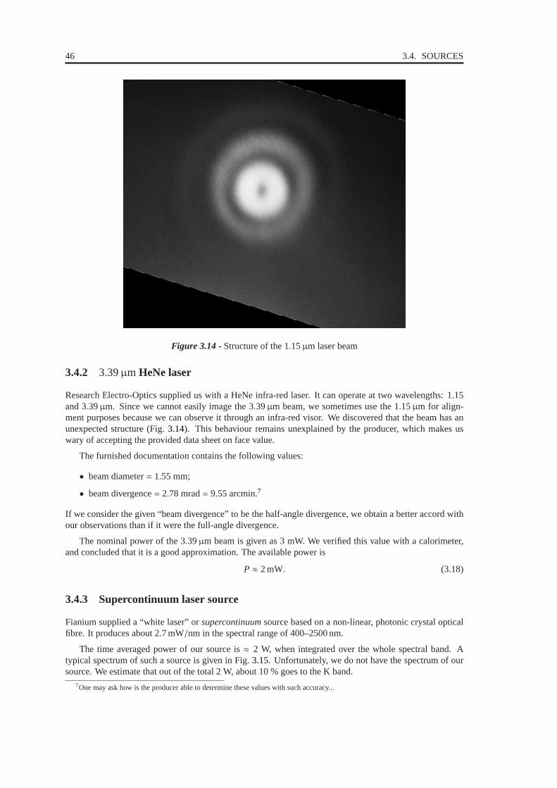
46 3.4. SOURCES
Figure 3.14 - Structure of the 1.15µm laser beam
3.4.2 3.39µm HeNe laser
Research Electro-Optics supplied us with a HeNe infra-red laser. It can operate at two wavelengths: 1.15and 3.39µm. Since we cannot easily image the 3.39µm beam, we sometimes use the 1.15µm for align-ment purposes because we can observe it through an infra-redvisor. We discovered that the beam has anunexpected structure (Fig.3.14). This behaviour remains unexplained by the producer, which makes uswary of accepting the provided data sheet on face value.
The furnished documentation contains the following values:
• beam diameter= 1.55 mm;
• beam divergence= 2.78 mrad= 9.55 arcmin.7
If we consider the given “beam divergence” to be the half-angle divergence, we obtain a better accord withour observations than if it were the full-angle divergence.
The nominal power of the 3.39µm beam is given as 3 mW. We verified this value with a calorimeter,and concluded that it is a good approximation. The availablepower is
P ≈ 2 mW. (3.18)
3.4.3 Supercontinuum laser source
Fianium supplied a “white laser” orsupercontinuumsource based on a non-linear, photonic crystal opticalfibre. It produces about 2.7 mW/nm in the spectral range of 400–2500 nm.
The time averaged power of our source is≈ 2 W, when integrated over the whole spectral band. Atypical spectrum of such a source is given in Fig.3.15. Unfortunately, we do not have the spectrum of oursource. We estimate that out of the total 2 W, about 10 % goes tothe K band.
7One may ask how is the producer able to determine these values with such accuracy...
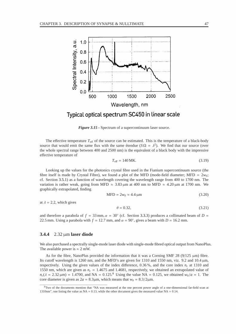
CHAPTER 3. DESCRIPTION OF SYNAPSE & NULLTIMATE 47
Figure 3.15 - Spectrum of a supercontinuum laser source.
The effective temperatureTeff of the source can be estimated. This is the temperature of a black-bodysource that would emit the same flux with the sameetendue (SΩ = λ2). We find that our source (overthe whole spectral range between 400 and 2500 nm) is the equivalent of a black body with the impressiveeffective temperature of
Teff = 140 MK. (3.19)
Looking up the values for the photonics crystal fibre used in the Fianium supercontinuum source (thefibre itself is made by Crystal Fibre), we found a plot of the MFD (mode-field diameter; MFD= 2w0;cf. Section3.5.1) as a function of wavelength covering the wavelength range from 400 to 1700 nm. Thevariation is rather weak, going from MFD≈ 3.83µm at 400 nm to MFD≈ 4.20µm at 1700 nm. Wegraphically extrapolated, finding
MFD = 2w0 ≈ 4.4µm (3.20)
atλ = 2.2, which givesθ = 0.32, (3.21)
and therefore a parabola off = 33 mm, α = 30 (cf. Section3.3.3) produces a collimated beam ofD =22.5 mm. Using a parabola withf = 12.7 mm, andα = 90, gives a beam withD = 16.2 mm.
3.4.4 2.32µm laser diode
We also purchased a spectrally single-mode laser diode withsingle-mode fibred optical output from NanoPlus.The available power is≈ 2 mW.
As for the fibre, NanoPlus provided the information that it was a Corning SMF 28 (9/125 µm) fibre.Its cutoff wavelength is 1260 nm, and the MFD’s are given for 1310 and 1550 nm, viz. 9.2 and 10.4µm,respectively. Using the given values of the index difference, 0.36 %, and the core indexnc at 1310 and1550 nm, which are given asnc = 1.4675 and 1.4681, respectively, we obtained an extrapolatedvalue ofnc(λ = 2.32µm) = 1.4700, and NA= 0.125.8 Using the value NA= 0.125, we obtainedw0/a = 1. Thecore diameter is given as 2a = 8.3µm, which means thatw0 = 8.3/2µm.
8Two of the documents mention that “NA was measured at the one percent power angle of a one-dimensional far-field scan at1310nm”, one listing the value as NA= 0.13, while the other document gives the measured value NA= 0.14.

48 3.5. MODAL FILTERS
We obtain thereforeθ = 0.178, (3.22)
which means that forf = 13 mm, andα = 35, the beam diameter isD = 5.1 mm.
3.5 Modal filters
We discussed the importance of wavefront filtering in nulling interferometry in Section2.5. While Salways used SMF’s, N, originally aiming for 10µm, is provided with a set of pinholes, and alsobenefited from the R&D on silver halide fibres at the University of Tel Aviv (prof. Abraham Katzir). Weare not working at 10µm, however.
3.5.1 Fluoride-Glass Single-Mode Fibres
We have five SMF fibres from Verre Fluore:
• two 1-metre K-band fibres with cutoff wavelengthλco = 1.95µm, and core diameter 2a = 6.5µm,
• three 2-metre K-band fibres,λco = 1.95µm, 2a = 6.5µm, and
• one 2-metre L-band fibre,λco = 2.85µm, 2a = 11µm.
The transmission of the fibres is shown in Figs.3.16, 3.17.
Our K-band single-mode fibre (SMF) has a numerical aperture (NA) of 0.23. This is given by thephysical properties of the materials used, namely
NA=√
n2core− n2
cladding. (3.23)
The waistw0 = 3.9µm, core diameter 2a = 6.5µm and normalised frequencyV = 2.135 atλ = 2.2µm.
Using
θ =λ
πw0(3.24)
we obtainθ = 0.18 rad= 10.3 (3.25)
for the far-field angular radius (half-angle divergence) ofthe Gaussian TEM00 beam at 1/e2.
3.5.2 Fibre output aperturing
An interesting option for the improvement of the modal-filtering performance of our fibres is output aper-turing (Lawson et al. 2008). With certain fibres (e.g., the silver halide fibres), pinholes may be installedrelatively easily on the exit fibrehead. Another approach isto collimate the output beam and use an iris inthe image plane.
3.6 Spectral filters
We are equiped with a set of interference filters furnished byNorthumbria Optical Coatings:
• two K filters with central wavelength of 2.21µm and full width at half maximum of 0.33µm, i.e.,2.045–2.375µm; bandwidth of 15 % (Fig.3.18);

CHAPTER 3. DESCRIPTION OF SYNAPSE & NULLTIMATE 49
Figure 3.16 - Transmission of the K-band single-mode fibre (in dB/km) vs. wavelength (inµm;courtesy VerreFluore).
Figure 3.17 - Transmission of the L-band single-mode fibre (in dB/km) vs. wavelength (inµm;courtesy VerreFluore).
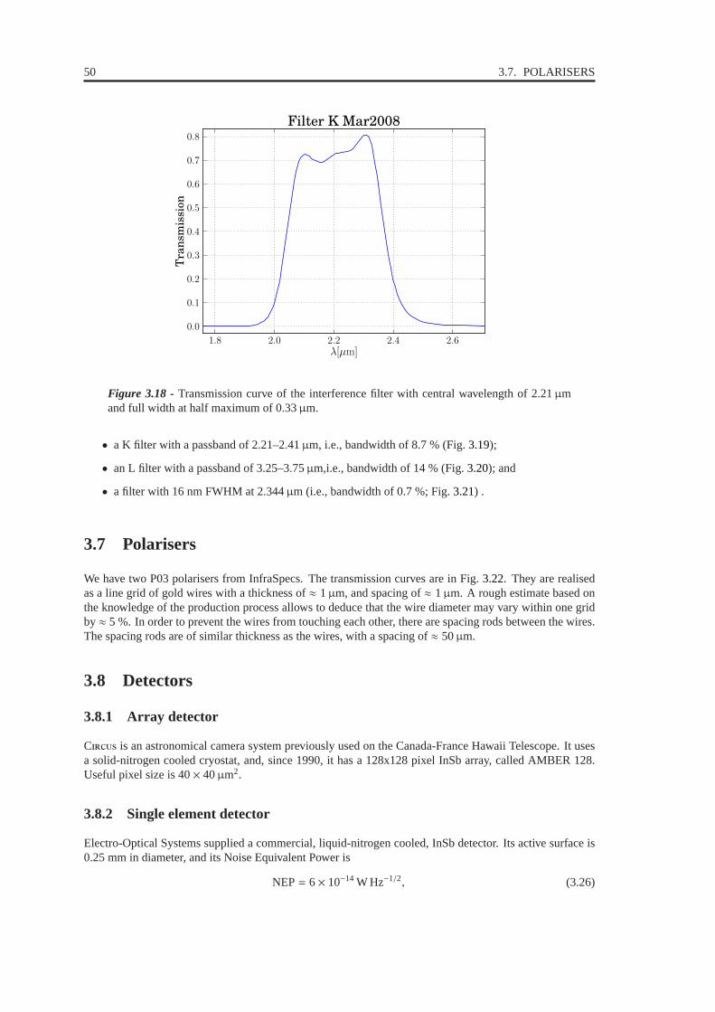
50 3.7. POLARISERS
Figure 3.18 - Transmission curve of the interference filter with central wavelength of 2.21µmand full width at half maximum of 0.33µm.
• a K filter with a passband of 2.21–2.41µm, i.e., bandwidth of 8.7 % (Fig.3.19);
• an L filter with a passband of 3.25–3.75µm,i.e., bandwidth of 14 % (Fig.3.20); and
• a filter with 16 nm FWHM at 2.344µm (i.e., bandwidth of 0.7 %; Fig.3.21) .
3.7 Polarisers
We have two P03 polarisers from InfraSpecs. The transmission curves are in Fig.3.22. They are realisedas a line grid of gold wires with a thickness of≈ 1µm, and spacing of≈ 1µm. A rough estimate based onthe knowledge of the production process allows to deduce that the wire diameter may vary within one gridby≈ 5 %. In order to prevent the wires from touching each other, there are spacing rods between the wires.The spacing rods are of similar thickness as the wires, with aspacing of≈ 50µm.
3.8 Detectors
3.8.1 Array detector
C is an astronomical camera system previously used on the Canada-France Hawaii Telescope. It usesa solid-nitrogen cooled cryostat, and, since 1990, it has a 128x128 pixel InSb array, called AMBER 128.Useful pixel size is 40× 40µm2.
3.8.2 Single element detector
Electro-Optical Systems supplied a commercial, liquid-nitrogen cooled, InSb detector. Its active surface is0.25 mm in diameter, and its Noise Equivalent Power is
NEP= 6× 10⁻¹⁴ W Hz−1/2, (3.26)

CHAPTER 3. DESCRIPTION OF SYNAPSE & NULLTIMATE 51
Figure 3.19 - Transmission curve of the interference filter with a passband of 2.21–2.41µm.
Figure 3.20 - Transmission curve of the interference filter with a passband of 3.25–3.75µm.
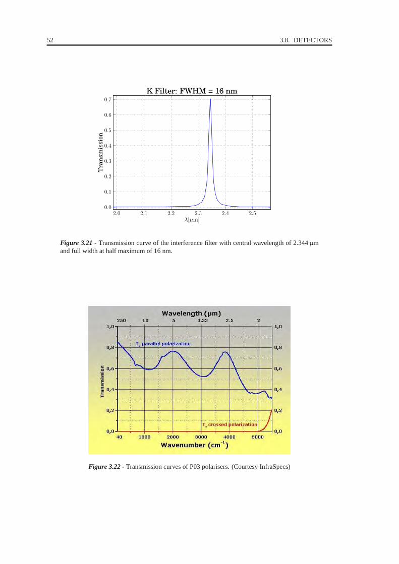
52 3.8. DETECTORS
Figure 3.21 - Transmission curve of the interference filter with central wavelength of 2.344µmand full width at half maximum of 16 nm.
Figure 3.22 - Transmission curves of P03 polarisers. (Courtesy InfraSpecs)

CHAPTER 3. DESCRIPTION OF SYNAPSE & NULLTIMATE 53
Figure 3.23 - Focus Crossing APS prototype
i.e., its specific detectivityD∗, consideringD∗ =√
A/NEP, whereA is the active area,
D∗ = 4× 1011 cm Hz1/2 W−1. (3.27)
3.9 Phase shifter prototypes
We have discussed the Achromatic Phase Shifters (APS) in Section 2.3. In the context of an ESA study, wehave three APS prototypes in addition to the CaF2-prisms forming an APS/chromatism compensator whichis an intrinsic part of the S testbed (cf. Sec.2.4).
3.9.1 Focus Crossing or Through Focus
A Focus Crossing APS prototype (APS FC; also known as ThroughFocus APS) was developed by theObservatoire de Cote d’Azur, Nice, France (Fig.3.23). The APS FC is based on the so-called Gouy effectwhere light undergoes a phase shift ofπ when crossing a focus. The phenomenon is independent of wave-length (Gouy 1890; Boyd 1980). The principle of this approach is similar to the one of the AchromaticInterfero-Coronagraph (Gay and Rabbia 1996; Baudoz et al. 2000a,b; Rabbia et al. 2006).
APS FC comprises two modules, one bearing two confocal half-parabolic off-axis mirrors, the other,two flat mirrors. The “confocal” module produces an achromatic π-phase shift, a pupil rotation byπ andan extra optical path (twice the focal length of a paraboloid), while the role of the “flat-flat” module is tobalance this pathlength and to reproduce the beam geometry of the confocal module. At beam combination,the resulting amplitude is nulled for an on-axis point-likesource, provided the wavefronts are perfectlycophased. If not, nulling is incomplete and a residual flux remains.
3.9.2 Field Reversal or Periscope
A Field-Reversal APS prototype (APS FR; also known as Periscope APS) is shown in Fig.3.24. The systemagain comprises two modules, but, unlike the APS FC where theflat-flat module is for reference purposesonly, here both modules are needed to create theπ phase shift. Each module is composed of three flatmirrors. Two reflections per beam are necessary to induce thephase shift, the third reflection merely flipsthe beams so that the outgoing beams are parallel to the incoming beams.
Two reflections, arranged in such a way thatsandp polarisation components are successively permuted,flip the field vectors, inducing an achromatic phase shift, aswell as a pupil rotation ofπ. Suitably appliedto a couple of beams, a couple of periscopes generates an intrinsically achromatic phase shift ofπ (opposedfield vectors). Then a modified constructive interferometerprovides two nulled outputs by suitably mixingthe beams.

54 3.10. ELECTRONICS & SOFTWARE
Figure 3.24 - Field Reversal APS prototype
Figure 3.25 - Dispersive Prisms APS prototype
A prototype APS FC was developed at Max-Planck-Institut fur Astronomie in Heidelberg in collabo-ration with Kayser-Threde GmbH in Munich and the IOF Fraunhofer Institute for Applied Optics in Jena(Launhardt 2008).
3.9.3 Dispersive prisms
The principle of this method consists in introducing dielectric plates into each arm of the interferometer.Their number, composition and thickness are optimised, together with the OPD, so that the chromaticityof the resulting phase shift in a given spectral band is belowa specified level. The description of S(Sec.3.11) mentions that a simple APS using two prisms of the same material in each arm of the interferom-eter is an integral part of the setup. A model with three prisms of three different materials per interferometerarm is under development by Thales Alenia Space. A set of three pairs of Dispersive Prisms was developedby Thales Alenia Space (Fig.3.24). The materials are Germanium, KRS5, and ZnSe.
3.10 Electronics & Software
We have already mentioned (Section3.8.2) the lock-in amplifier which is a fast and sensitive Analog-DigitalConverter (ADC) with a precision oscillator and a computer running sophisticated software. But we shallnot go into the details of the commercial hardware with its built-in software. Rather, we shall concentrateon the custom software used in experiment control and data acquisition.

CHAPTER 3. DESCRIPTION OF SYNAPSE & NULLTIMATE 55
Figure 3.26 - Stanford Research Systems SR830 Lock-In Amplifier.
3.10.1 Lock-in amplifier
3.10.1.1 Data sampling or transfer?
The Stanford Research Systems SR830 Lock-In Amplifier (Fig.3.26) operates digitally, i.e., after it digitisesthe input signal all of its further operation is digital. Thedata output stream is accessible via a GPIB port. Adigital-analog converter is built in to provide an optionalanalog output, coding the output data as a voltage.Its mainraison d’etreis backwards compatibility: lock-in amplifiers’ operationused to be analog, and itwas therefore natural to use an analog output port. With a fully digital lock-in amplifier this does not makesense.
The argument for keeping with the analog output is that the digital data transfer is too slow. This lineof thought ignores the fact that there is a fundamental difference between the data output of an analog anda digital lock-in amplifier. In the days of analog lock-in amplifiers the output was a raw stream, and it wasup to the user to treat it. A fully digital lock-in amplifier, on the other hand, provides a clean digital outputthat does not have to be faster than, typically, the time constantτ. It does not make sense to acquire data ata frequency higher than 1/τ because the output data stream does not require any processing (fast sampling,averaging, etc.): all that has already been done by the lock-in amplifier much more cleanly than whateverthe user can do playing with the re-analogised voltage. What happens between the lock-in amplifier and theexperiment-control computer is data transfer, not data sampling. Sampling is done by the lock-in amplifier’sanalog-digital converter operating on the input signal.
The original S architecture uses the old way of thinking about lock-in amplifiers. It is only thelatest system, which we implemented on the N testbed in 2008/2009, that uses the digital outputdirectly. S II therefore uses the re-analogised lock-in amplifier output sampled by an external analog-digital converter (we use commercial products of theNational InstrumentsCorporation).
3.10.1.2 “Dark current”
The lock-in amplifier’s output is a complex value represented as two real numbers. This ordered pair ofnumbers is provided either in its native Carthesian form, viz., asX and Y, or converted into polar co-ordinate system, asR andθ. The lock-in amplifier represents the data in the Carthesianform, and providesthe conversion to polar co-ordinates as an optional step. Itis therefore faster (albeit marginally) to workwith X andY.
When the lock-in amplifier operates with a chopper wheel (as inour case), it receives alternatively thebackground flux alone and the signal with the background. Itsoutput can be naturally viewed as a resultof a sophisticated method of subtracting the background from the signal. Contrary to many experimenter’sreflexes, it is therefore unnecessary to subtract a “dark current”. It has already been done by the lock-in

56 3.10. ELECTRONICS & SOFTWARE
amplifier.
Another way of looking at this issue has to do with the behaviour of the co-ordinateθ. It has two regimesof behaviour:
1. When there is a signal (when there is a consistant difference between the voltage acquired when thechopper wheel leaves the beam path open, and when it shuts it)thenθ fluctuates around a determinedvalue with an amplitude of, typically, a degree.
2. When there is no signal (no consistant difference between the situations when the chopper wheelopens and closes the beam path) then the value ofθ is uniformly distributed over 2π.
Naturally, the value ofR has a different physical interpretation in the two cases. In the first instance, it is agood estimate of the signal (unless the signal-to-noise ratio is very poor, e.g.,< 2). In the second instance,it is the modulus of two random variables,X andY, which are both supposed to have zero mean values,〈X〉 = 〈Y〉 = 0. What we would really like to know is notR, but rather we would like to verify that indeed〈X〉 = 〈Y〉 = 0, and to determine the standard deviationsσX, σY. MeasuringRcan merely provide an upperlimit on these values.
3.10.2 Software
As with the testbeds themselves, our custom software went through several stages of development. The firstsystem, implemented on the S testbed, was developed by Frank Brachet. It was entirely implementedusing theNational InstrumentsLabView software (for more details seeBrachet(2005)). The perceivedpriority in the design of this system was the integration of the metrology feedback loop, requiring fast,real-time operation with high data transfer rates.
Once it was realised that the metrology system will no longerbe a concern, other issues came to theforefront. The main weakness of the Frank Brachet’s system was that new functions were difficult andtedious to implement. Therefore, a more flexible architecture was desired.
This second stage of software development was based on the system implemented on the S testbedat the Observatory of Paris in Meudon. The basic issue this system set out to address in Meudon was remoteoperation: the laboratory being relatively far from the offices of the experimentators, an efficient method ofrunning the setup remotely became a priority. The solution was to create a simple server that would receivecommands via ethernet. The server was implemented using LabVIEW, while the commands were sent (andresponses were received) through shells running IDL, Yorick, MatLab, etc.
The S architecture was adapted at IAS by Bruno Chazelas and myself, the one major differencebeing that the user interface shell was written in Python.
The third stage is an upgrade of the previous S-based design. There are two key differences.Firstly, the data acquisition via the lock-in amplifiers wasoverhauled, making it purely digital. And sec-ondly, the concept of remote operation shifted.
The original S design had the server software running on a computer in the laboratory and the userinterface running on a computer in a distant office. Over time we started relying more and more on VNC9,i.e., on remote desktop sharing software. We would run both the server and the user interface software onthe same computer in the experiment’s control room, bringing up this computer’s desktop remotely via VNCon any computer connected to the network. The obvious advantage of this solution is that the user interfacesoftware needs to be installed and kept up-to-date only on one computer, which facilitates tweaking of thesoftware.
This changed mode of operation brought about a change in the division of labour between the serverand user interface software.
9Virtual Network Computing
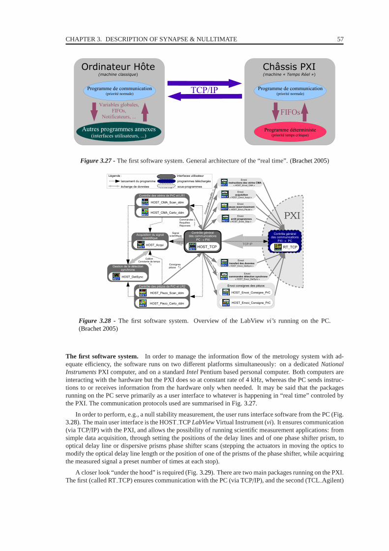
CHAPTER 3. DESCRIPTION OF SYNAPSE & NULLTIMATE 57
Figure 3.27 - The first software system. General architecture of the “realtime”. (Brachet 2005)
Figure 3.28 - The first software system. Overview of the LabViewvi’s running on the PC.(Brachet 2005)
The first software system. In order to manage the information flow of the metrology system with ad-equate efficiency, the software runs on two different platforms simultaneously: on a dedicatedNationalInstrumentsPXI computer, and on a standardIntel Pentium based personal computer. Both computers areinteracting with the hardware but the PXI does so at constantrate of 4 kHz, whereas the PC sends instruc-tions to or receives information from the hardware only whenneeded. It may be said that the packagesrunning on the PC serve primarily as a user interface to whatever is happening in “real time” controled bythe PXI. The communication protocols used are summarised inFig. 3.27.
In order to perform, e.g., a null stability measurement, theuser runs interface software from the PC (Fig.3.28). The main user interface is the HOSTTCPLabViewVirtual Instrument (vi). It ensures communication(via TCP/IP) with the PXI, and allows the possibility of running scientific measurement applications: fromsimple data acquisition, through setting the positions of the delay lines and of one phase shifter prism, tooptical delay line or dispersive prisms phase shifter scans(stepping the actuators in moving the optics tomodify the optical delay line length or the position of one ofthe prisms of the phase shifter, while acquiringthe measured signal a preset number of times at each stop).
A closer look “under the hood” is required (Fig.3.29). There are two main packages running on the PXI.The first (called RTTCP) ensures communication with the PC (via TCP/IP), and the second (TCLAgilent)

58 3.10. ELECTRONICS & SOFTWARE
Figure 3.29 - The first SW system. Overview of the LabViewvi’s running on the PXI. (Brachet2005)
is the “real-time” loop designed for theAgilent metrology control system. The loop has many operatingmodes (represented by different CASEs in thevi) which are selected, according to the information comingfrom the user interface.
The metrology loop was an essential element of the TCLAgilent, and was running permanently when-ever the software was on. Nonetheless, the loop could run without actually effecting any changes in theposition of the delay lines. In this case, the loop was merelymonitoring the metrology signal, opening thepossibility of recording the OPD information. As we have already mentioned (Section3.3.6.3), this settingwas the only viable option because the metrology beams passed above the science beams, and thereforethe metrology was following the mechanical vibrations of the optics at inappropriate points of incidence.In fact, simple geometrical considerations give credibility to the opinion that the vibration amplitude at thetwo levels must have been different (viz., roughly twice larger at the metrology level than at the sciencebeam level).
The first version of the OPD dithering algorithm (see Chapter4) was implemented under this system,in a subset of the CASEs mentioned above.
The second software system. Inheriting theNational InstrumentsPXI industrial computer with all of theinput/output operations from/to the testbed being handled by the PXI’s cards, meant that the new Sserver (introduced in Section3.10) had to be installed on the PXI. These machines, however, aredesignedwith a different mode of operation in mind, viz., they are furnished with a minimalist operating system thesole purpose of which is to run compiled LabVIEW programmes,loaded via ftp. It was decided to makeour PXI double boot, i.e., adding the option of running Windows XP for more flexibility.
The S server LabVIEW vi (virtual instrument) runs a loop waiting for messages sent to it viaethernet (TCPIP, Fig.3.30). Each message is decoded as a string of characters. If the first eight characterscorrespond to one of the implemented instructions (see Table 3.1), the appropriate code is executed and aresponse (if any) is sent out again as a string of characters via ethernet.
The framework of the server was taken from the S software but the commands were implementedfrom scratch.
At this stage, the philosophy of the server LabVIEW vi closely copied that of our colleagues in Meudon:the user was not to use the server’s front end directly, but rather interact with a shell (written in a scripting

CHAPTER 3. DESCRIPTION OF SYNAPSE & NULLTIMATE 59
Figure 3.30 - The second software system. The server LabVIEWvirtual instrument, based onthe loop designed for the S testbed at the Observatory of Paris in Meudon (left), runs ona dedicated PXI industrial computer hard-connected to the systems of the testbed. It receivescommands and sends out answers via TCP-IP to and from a Pythonshell (right) implemented onany user computer. The server itself does not provide directdata output.
Command Description
CMDSR830 General communication with the lock-in amplifier.LIA MMSR Versatile measurement with lock-in amplifiers.MSR REG1 An acquisition of the lock-in amplifier data output.GET DETS Get lock-in amplifier’s gain.SET DETS Set lock-in amplifier’s gain.GET OFLT Get lock-in amplifier’s time constant.SET OFLT Get lock-in amplifier’s time constant.ADJ DETS Adjust lock-in amplifier’s gain to a given voltage.SRC DETS Adjust lock-in amplifier’s gain to the signal.CMND SMC General communication with the SMC commander.NSC CMND General communication with the NSC commander.ROT SHUT Open or close one or both interferometer branches.
Table 3.1 - The second and third software system. List of commands implemented in the Sserver (a sample).

60 3.11. SYNAPSE
language), sending commands, receiving and visualising the testbed’s response in the shell environment.
The shell Bruno Chazelas and myself implemented, is writtenin Python. Its basic module deals with thecommunication via TCP-IP with the server LabVIEW vi. Another module wraps the server’s eight-charactercommands, generating the appropriate strings (comprisingthe command and its arguments) to be sent to theserver, providing default arguments, screening the user input for invalid argument values, and decoding theserver’s response, converting the incoming string of characters into appropriate variables. The third moduleis a collection of scripts calling the commands, wrapped by the previous module, in order to perform moresophisticated operations (e.g., flux mismatch estimate, which requires alternate measurements of the flux ineach branch of the interferometer).
The fact that our work isresearchin the ethymological sense, made itself manifest also in theprocessof software development. In fact, with time it became clear to us that our practice comprises three stages:
1. First we would try a new experimental procedure sending out commands one by one, manually typingthem in through the shell.
2. Once we had a good grasp of an algorithm we would write a Python script and include it as a method,usually, in the “tools.py” module.
3. After a while we might find that it would be better to implement the same function directly as one ofthe commands of our S LabVIEW server.
A good example of this process is the procedure providing an estimate of intensity mismatch (Section3.3.5).
The OPD dithering algorithm was implemented in this versionof the software as a separate programthread, comprising a loop, initially running “dry” (without performing any action) and accepting threedifferent commands: (1) start dithering or restart it after a pause, (2) pause dithering, and (3) stop ditheringclosing down the thread. Each of these commands took additional arguments defining the duration of theindividual stages of the dithering cycle, etc.
The third software system. The third software system can be called a consequence (if somewhat belated)of fast networking. It took us a while to realise the obsolescence of the San philosophy, which solvedthe conundrum of remote experiment control by running a server and a shell on two different computerslinked via TCP-IP. Fast networking makes it easy to run both the server and the shell on the same ma-chine, which the user interacts with via a remote desktop session (including work from off-campus homecomputers).
The advantage of this system is very practical: The originalS system was a little cumbersome todevelop because software versions had to be carefully correlated between the dedicated PXI and the usermachines running the Python package. It required additional work to keep track of the development andco-ordinate the work. What is more, the “viewer” module, providing graphics output in the Python shell,was liable to platform-related and installation-related instabilities. With both the server and the commandshell running on the same machine, all of these problems wereeliminated.
Working via remote desktop also had some other implications, the main one being that the graphicsoutput could be implemented directly on the LabVIEW server level. This is clearly a more logical solutionbecause there is no need of data transfer via the TCP-IP protocol10.
3.11 S
Fig. 3.32shows the interferometer with the science and metrology beams. It is set up on an optical tablewith passive vibration protection, and protected from acoustic and thermal perturbations by a plexiglass box(Section3.3.6.1). The optical bench itself comprises two modified Mach-Zehnder interferometers serving
10The transfer is internal to the same computer but it still passes through the ethernet card.

CHAPTER 3. DESCRIPTION OF SYNAPSE & NULLTIMATE 61
Figure 3.31 - The third software system. The server LabVIEWvirtual instrument, based on theloop designed for the S testbed at the Observatory of Paris in Meudon (top left), runs ona dedicated computer hard-connected to the systems of the testbed. It receives commands andsends out answers via TCP-IP to and from a Python shell (top right) implemented on the samecomputer. The server also provides direct output of data in graphic form. The user communicateswith the system via remote desktop (VNC; bottom).

62 3.11. SYNAPSE
Figure 3.32 - Images of S overlaid with science and metrology beams

CHAPTER 3. DESCRIPTION OF SYNAPSE & NULLTIMATE 63
Figure 3.33 - Metrology beam splitter.
as beam-splitting and beam-recombination devices (Serabyn and Colavita 2001), creating the two identicalbeams (Section3.3.4), delay lines, and a simple APS with two CaF2 Prisms in each interferometer arm.
The beam-splitter and beam-combiner systems use parallel CaF2 plates. Their thickness is not guaran-teed to be identical to the required accuracy, and thereforea compensator needs to be included in the design.The bench’s intrinsic APS, comprising two CaF2 prisms in each interferometer arm, fulfills this role. Asan APS, it can introduce any given phase shift, and reduces the chromaticity in the K or L band so that theresulting theoretical nulling performance is better than≈ 10−5.
The metrology beam (Section4.2) is generated by a laser (under the optical table) and split by a ded-icated beam splitter (Fig.3.33) which is suspended from the top of the tower also housing thefirst beam-splitting plate (Fig.3.32, the tower is in the bottom-left corner of the beam-splitter’s breadboard).
Both delay lines, based on rooftop mirrors, are motorised:
• one with a stepper motor running 25 mm (i.e., optical path of 50 mm) at 0.1µm reproducibility,
• and the other with a piezoelecric actuator running 15µm at a reproducibility better than 0.5 nm.
Since the bench (if well aligned) is symmetric by design, theflux of the two arms can be balanced usingsimply injection into the exit SMF, tweaking the orientation of the folding mirror illuminating the off-axisparabola (Section3.3.5). The better the superposition of the two beams, the easier the balancing.
3.12 S II
The functional outline of the S II testbed is given in Fig.3.34. It is very similar to the originalS, differing only in four aspects:
• the external-metrology system was dismounted,
• there was extensive work done on the mechanics (e.g., the optical table was changed, the tower on the

64 3.13. NULLTIMATE
Figure 3.34 - S II (from left to right): Sources (three options), SMF, beam-splitter subsys-tem, CaF2 prisms (chromatism compensator and/or APS), optical switch, APS prototype modules,beam-combiner subsystem, SMF, detectors (two options).
beam splitter’s breadboard was disassembled, the beam combiner was placed on a new breadboard),enabling us to improve the alignment,
• the Focus Crossing APS prototype was mounted, and
• new sources were coupled to the input fibre (S originally used only the Ceramic Black Body).
For the tests of the FC APS prototype, a translation stage with folding mirrors acts as an optical switchto insert the prototype into the optical path.
3.13 N
The general optical layout of N (Fig.3.35) is that of a simple Mach-Zehnder interferometer, ratherthan a double one as is the case with S. The number of optical surfaces has been reduced. Theoptics are ZnSe. The beam splitter and the beam combiner are prismatic (1 opening angle) and requirecompensators (Section3.3.4). One of the compensators is also a chromatism compensator (Section3.3.7).The mechanical design uses a line-point-plane on all optical elements (Fig.3.36).

CHAPTER 3. DESCRIPTION OF SYNAPSE & NULLTIMATE 65
Figure 3.35 - N: outline of the optical layout. The beam arrives from bottomright,going left towards two folding mirrors and a parabola which injects it into the input fibre. Thebeam leaves the diagram at top left.

66 3.13. NULLTIMATE
Figure 3.36 - N. The line-point-plane system is implemented on all opticalelements.
Chapter 4Stabilisation
Contents4.1 Introduction . . . . . . . . . . . . . . . . . . . . . . . . . . . . . . . . . . . . . . . . . 67
4.2 Metrology . . . . . . . . . . . . . . . . . . . . . . . . . . . . . . . . . . . . . . . . . . . 68
4.2.1 Setup and operation. . . . . . . . . . . . . . . . . . . . . . . . . . . . . . . . . . 68
4.2.2 Results . . . . . . . . . . . . . . . . . . . . . . . . . . . . . . . . . . . . . . . . 68
4.3 Optical Path Difference Dithering . . . . . . . . . . . . . . . . . . . . . . . . . . . . . 68
4.3.1 Introduction. . . . . . . . . . . . . . . . . . . . . . . . . . . . . . . . . . . . . . 68
4.3.2 Principle . . . . . . . . . . . . . . . . . . . . . . . . . . . . . . . . . . . . . . . 70
4.3.3 Cycle parameters. . . . . . . . . . . . . . . . . . . . . . . . . . . . . . . . . . . 70
4.4 Results . . . . . . . . . . . . . . . . . . . . . . . . . . . . . . . . . . . . . . . . . . . . 72
4.4.1 K band . . . . . . . . . . . . . . . . . . . . . . . . . . . . . . . . . . . . . . . . 72
4.4.2 Laser light . . . . . . . . . . . . . . . . . . . . . . . . . . . . . . . . . . . . . . 75
4.5 Comparison with some other experiments. . . . . . . . . . . . . . . . . . . . . . . . . 77
4.6 Discussion . . . . . . . . . . . . . . . . . . . . . . . . . . . . . . . . . . . . . . . . . . 77
4.1 Introduction
We have seen (Sec.2.6) that stability is crucial for nulling interferometry. Testbed studies suggest that it isnot easy to achieve.
OPD is one of the first quantities that needs to be controlled in an interferometric setup. Several strate-gies may, and in fact, should be applied simultaneously. Oneapproach uses a separate metrological servosystem, based on a laser beam following the path of the beam whose behaviour is actually under study (“sci-entific beam”) as closely as possible. The strong points of such systems include high accuracy, monitoringas well as servo functions, high-frequency servo control, etc. The disadvantages have to do with the factthat metrology always uses monochromatic lasers whereas the scientific beam ultimately has to be a poly-chromatic one. Moreover, the metrological laser is very often at a wavelength outside of the working bandof the experiment, which means that the OPD’s and the flaws seen by the two systems may be different.
An alternative approach is dither stabilisation, implementing a servo mechanism based on the scientificbeam itself. A classical form of this technique has been investigated byOllivier et al. (2001), although thisfirst experiment was inconclusive. More recently,Schmidtlin et al.(2005) have demonstrated the potentialof dithering in a sequential way, obtaining good levels of stabilisation with nulling ratio around 8 10−7 witha laser diode at 638 nm. It was this work that provided our teamwith decisive inspiration.

68 4.2. METROLOGY
4.2 Metrology
In the original concept of S, a dedicated metrology system was to monitor and control OPD. Themetrology system is a Michelson interferometer based on a commercial product (HP Agilent 10716A)operating with visible laser beams (HeNe 633 nm) that run four times through the setup. This ensuresa precision of 0.3 nm. The drawback is that the metrology beams cannot easily follow exactly the samepath as the science beams (mainly because of the fundamentaldifference between a Mach-Zehnder and aMichelson setup). Fig.3.32shows the metrology beams running about an inch above the science beams.The optical path comprises 16 reflections and 19 transmissions in each arm; and the metrology beams passthrough them four times.
4.2.1 Setup and operation
The electric signal produced by the metrology detector is digitised by the electronics of a commercial PCIcard. The output of the card is a 32-bit channel at 10 MHz. Eachof these 232 steps corresponds to 0.3 nm.The system is thus capable of measuring distances of about 1.3 m with a resolution of 0.3 nm.
Since the optical properties of the testbed are not likely tochange on timescales of 1/10MHz= 0.1µs,the output is too fast. What is more, the piezzoelectric actuator of the Fine Delay Line which is in the servoloop, is not designed to operate at such timescales. The PCI card’s output, therefore, is averaged by customelectronics before entering the computer that runs the 4-kHz control loop .
4.2.2 Results
In 2005 S in this setup reachednl = 3× 10⁻⁴ in the K band. It also became clear that there was asignificant OPD drift.
Let us reproduce the results of two typical acquisitions without stabilisation. The first (Fig.4.1, left)shows an acquisition of about 200 s with a mean nulling ratio〈nl〉 = 2.7 10−4 with a considerable standarddeviationσ〈nl〉 = 6 10−5. The second (Fig.4.1, right) is a slightly longer recording, of about 10 minuteswith a nulling ratio〈nl〉 = 2.5 10−4 during the first 100 seconds (withσ〈nl〉 = 6 10−5), showing the effects ofsignificant drift, probably due to OPD instability.
Applying metrology stabilisation did not help, unfortunately. Fig.4.2shows a data acquisition obtainedwith the metrology running. A drift quite clearly persists.
4.3 Optical Path Difference Dithering
4.3.1 Introduction
Dithering is a standard technique in control engineering defined as “the modification of the low-frequencyproperties of an unstable nonlinear system by the application of a high-frequency signal in order to stabilisethe system” (Gelb and Vander Velde 1968).
The present algorithm, however, departs in two ways from theclassical system described by the quoteddefinition (the very formulation of which is reminiscent of analog electronic signal processing). First, thegoal of the classical dithering method is to obtain a deconvolved signal: the dithered parameter is changingcontinuously, and the measured signal is a convolution of the variations due to the dithering as well as dueto the studied system.
In our case, the experimental setup displays good stabilityon intermediate time scales (t < 100 s), andwe only have to fight against long-term drifts. Our approach was, therefore, to reach and maintain a delay-line positionx0 corresponding to the best null simply by moving the delay line every few seconds, rapidlymeasuring the flux at positionsx0± ε, and moving the delay line to a new position based on the information

CHAPTER 4. STABILISATION 69
Figure 4.1 - S measurements in the K spectral band. Left: The transition between thebright fringe (the first 50 seconds) and the dark fringe (between 50 s and 240 s) was performedmanually by modifying the length of the delay line. The last part of the curve shows the darkcurrent (the detector being covered). The mean rejection factor is about 2.4 times greater than thedark current of the detector. Right: Same measurement with asignificant drift.
Figure 4.2 - S measurement in the K band with the external metrology systemrunning. Adrift is clearly present.

70 4.3. OPTICAL PATH DIFFERENCE DITHERING
obtained during these excursions. UnlikeSchmidtlin et al.(2005) who record data throughout the ditheringcycle (i.e., their recorded data contain points measured during delay-line movement and point measured atx0 ± ε), we chose to investigate a slightly different approach and to record data only during the final stageof each dithering cycle (i.e. atx0), corresponding to the best null.
Thus, the second difference between our procedure and the classical definition ofdithering is that wedo not have to perform any post-acquisition signal deconvolution. Our version of dithering simply helps tomaximise the amount of time the system stays in its optimal setting; i.e. employing the dithering only whenneeded, with relatively long periods of unperturbed data acquisition.
4.3.2 Principle
The nulling ratio in the vicinity of the dark fringe’s centre, with other parameters constant, can be describedas a function of the phase shift∆ϕ (Eq.2.14):
nl =Imin
Imax=
1+ cos(π + ∆ϕ)1+ cos(∆ϕ)
=1− cos(∆ϕ)1+ cos(∆ϕ)
(4.1)
nl ≈1− 1+ ∆ϕ
2
2
1+ 1− ∆ϕ2
2
≈ ∆ϕ2
4for ∆ϕ ≪ 1. (4.2)
Bracewell’s method uses achromatic phase shifters (APS) toproduce aπ phase shift independent of wave-length (within a given band). The phase shift can be translated into the OPD between the two arms of theinterferometer
∆ϕ(λ) = 2πxλ
(4.3)
wherex is the OPD. The signal during an OPD scan can be described as tracing a parabola around the pointwhere the nulling ratio reaches its minimum versusλ (x≪ λ)
I = ax2 + bx+ c. (4.4)
The vertex of the parabola corresponds to the deepest null obtainable at a given moment adjusting thedelay line, i.e. the centre of the dark fringe. The drift in nulling performance due to OPD instability cantherefore be represented as a shift of the parabola and of itsvertex.
With the empirical knowledge of three points of a parabola wecan calculate the position of its vertexunambiguously. Since measurement of three points of the parabola is required, the OPD has to be modifieddeliberately. In our experimental setup the speed of operations is limited by the speed of the delay lineactuators and by the integration time required to get a sufficient signal-to-noise ratio. This allows forcompensation of slow drifts (observable on time scales of a few tens or hundreds of seconds).
If data are acquired at three different OPD’s, e.g. atx0, x0 + ε, andx0 − ε, then the position of the darkfringe, i.e. of the vertexxv of the parabola, can be calculated as
xv = x0 −I+ − I−
2(I+ + I−) − 4I0ε (4.5)
whereI0, I+, and I− are the signal values measured atx0, x0 + ε, andx0 − ε, respectively. This formularepresents a simple recipe that can be directly implemented(Fig. 4.3).
4.3.3 Cycle parameters
The choices of dithering-cycle parameters are a result of several trade-offs.

CHAPTER 4. STABILISATION 71
Figure 4.3 - OPD dithering cycle. The top curve shows schematically the position of the delayline whereas the bottom curve is an idealised representation of the corresponding detected signal.From an initial position the dithering alters the OPD value by +ε(OPD) with respect to the initialposition. A measurement of the flux is performed. During the next stage, the dithering algorithmagain alters the OPD, this time by−ε(OPD) with respect to the initial position. Another measure-ment is performed. We thus know three points, defining a parabola (right), which allows us tocalculate and reach a new working position of the OPD (the vertex of the parabola).
4.3.3.1 Waiting times
A limitation is imposed by the delay line’s movement. The piezzoelectric actuator reaches a position closeto the desired one very rapidly, but then its controller takes some time, proportionate to the movement’samplitudeε, to stabilise the system at the new position:
τDL ≈(
90+ 6ε
nm
)
ms. (4.6)
Forε of 5 nm, each dithering cycle therefore implies a waiting time of:
3τDL(ε = 5 nm) ≈ 360 ms (4.7)
4.3.3.2 Dithering amplitude
As for the dithering amplitudeε itself, we accepted a limitation imposed by the gauge of the data acquisitionsystem. We used a lock-in amplifier (Section3.10.1) and, since changing its gauge requires time, wemaintained the same gauge for all measurements: atx0, x0 ± ε andxv, alike.
The flux I±(ε) measured atx0 ± ε can be approximated as
I±(ε) ≈ Imax∆ϕ2
4= Imax
(
πε
λ
)2, (4.8)
whereas the flux atxv, expressed asImaxnl, (4.9)
is due to a residual flux mismatch between the two arms of the interferometer, polarisation issues, and otherfactors contributing to nulling degradation. On the whole,we found that
ε = 5 nm (4.10)
∆ϕ = 1.5 10−2, (4.11)
was well suited for our purposes.

72 4.4. RESULTS
4.3.3.3 Integration time
The dithering cycle with a duration ofτcyc can be regarded as comprising:
• integration timeτv at xv, and
• timeτcyc− τv when dithering actions are performed.
The noise (assuming it is white noise in the relevant frequency band), measured by the standard devia-tionσ, decreases with the square root of the integration time. Thescaling factor forσ is therefore
√
τcyc
τv. (4.12)
If τv/τcyc = 2/3, the noise will increase by 22 %. Ifτv/τcyc = 9/10, the noise will increase by 5 %.Therefore, in our experiment we did not consider it a strong priority to increaseτv/τcyc beyond≈ 2/3.
4.3.3.4 Integration time at auxiliary points (xv ± ε)
There are two possible upper limits for the integration timeτ± of the flux I± measurements atxv ± ε.
• One is given by the fact that there is no reason for the corresponding SNR to be better than that of theflux Iv measurements atxv. This can be expressed as (assuming white noise only):
τ± ≤ τvIv/I± = τv 4nl/∆ϕ2 (4.13)
• The second upper limit forτ± to be considered is given by the timeτDL taken up by delay-linemovements.
As a rule of thumb, since it takesτDL to reach a position, there is little practical gain in reducing τ±to values less thanτDL, which leads toτ± ≤ τDL. In practice, it is this latter upper limit that will be moreapplicable.
4.4 Results
We have tested this method on the S testbed, and found it very convenient to use. It is highly efficientin finding the physical dark fringe (within one or two iterations; Fig.4.4, left) and reliable, driving the OPDback to its optimal value in spite of artificial perturbations (Fig.4.4, right).
4.4.1 K band
We performed three long dithering-stabilised data acquisitions, two of more than 6 hours each, and one of2 hours 20 minutes. All three were performed with comparablesettings: 1.25 s per stage, i.e.,τ± = τv =1.25 s, and 6.25 s per cycle1; dithering amplitudeε = 5 nm, i.e.,∆ϕ = 1.5 10−2; lock-in amplifier’s timeconstant at 100 ms.
The fluxes in the two arms of the interferometer were balancedbefore the acquisition (using an ad-justable semi-planar knife-edge) with an accuracy better than 0.5 percent.
Fig. 4.5 presents one of the 6-hour data acquisitions, together withdata taken immediately before thestabilisation was turned on and after it was turned off. Drifts are quite clearly present without the stabilisa-tion.
1At this point the dithering cycle could not be optimised, the control software allowing only for stages of equal duration (cf. Gabor2006).

CHAPTER 4. STABILISATION 73
Figure 4.4 - Oscilloscope measurements.
(a) Nulling rationl from a 6 hour-long OPD dither-stabilised data acquisition
(b) Data acquisition with no stabilisation taken before andafter the long sta-bilised run
Figure 4.5 - (a) Nulling ratio (or stellar leakage)nl(t) as a function of time (blue plot), with themoving average calculated over 625 seconds〈nl(t)〉625s overplotted (red). (b) Data acquisitionswith no stabilisation taken immediately before and after the long stabilised run.

74 4.4. RESULTS
Figure 4.6 - Left: Power spectrum density of the nulling function, PSD(nl). Note that 1/ f com-ponent is negligible. Right: Standard deviations of the running average of the nulling functionover the time intervalτ, σ〈nl〉(τ) (curve above). A (displaced)τ−1/2 function is shown for compar-ison (line below). Note that up toτ ≈ 500 s, the experimental curve is consistent with theτ−1/2
behaviour, withσ〈nl〉(500 s)≈ 1.5 10−5.
With no beams, the lock-in amplifier’sθ output was random, and the mean values of theX andY outputs
〈X〉 ≈ 〈Y〉 ≈ 0 (4.14)
This means that the measurement chain was well set up. Since the standard deviations of theX andYoutputs
σX ≈ σY ≈ 0.2µV, (4.15)
the acquiredRoutput was more than 10 times greater, and therefore this output can be considered to repre-sent the measured flux directly (without “subtracting the dark current”; cf. Section3.10.1.2).
The bright-fringe signal was thusImax = (8.4± 1.0) mV (4.16)
and the dark-fringe signal wasImin = (4.0± 1.1) µV (4.17)
The mean nulling rationl was, therefore
〈nl〉 = (4.7± 1.4)10−4 (4.18)
In order to evaluate the nulling ratio’s variability, we looked at its Power-Spectrum Density (PSD) and atthe standard deviation as a function of integration time. Fig. 4.6(left) shows the power-spectrum density ofthe nulling function, PSD(nl), while Fig.4.6 (right) shows the standard deviation of the mean value of thenulling function over the time intervalτ, σ〈nl〉(τ).
Let us now briefly list the results of this analysis. We shall discuss them in due course (Section4.5).Note, however, that there is no significant 1/ f component in the PSD plot (Fig.4.6), and the standarddeviation decreases with integration time asτ−1/2 up toτ ≈ 600 s. (Fig.4.6).
The main result can therefore be stated in terms of the standard deviation of the mean nulling ratioaveraged overτ = 600 s (analysing a set of mean values for the integration timeof τ = 600 s where thesemeans correspond to a moving window2):
σ〈nl〉(τ = 600 s)≈ 1.5× 10⁻⁵. (4.19)
2This type of statistics is called themovingor running average.
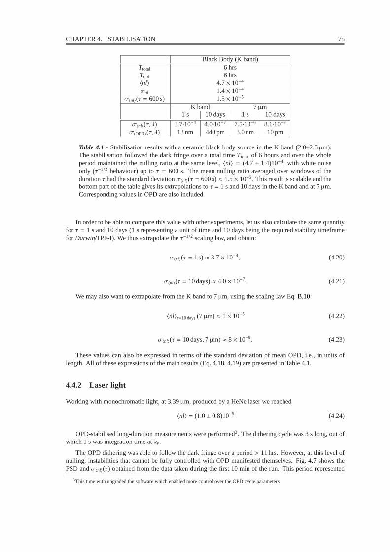
CHAPTER 4. STABILISATION 75
Black Body (K band)Ttotal 6 hrsTopt 6 hrs〈nl〉 4.7× 10⁻⁴
σnl 1.4× 10⁻⁴
σ〈nl〉(τ = 600 s) 1.5× 10⁻⁵
K band 7µm1 s 10 days 1 s 10 days
σ〈nl〉(τ, λ) 3.7·10−4 4.0·10−7 7.5·10−6 8.1·10−9
σ〈OPD〉(τ, λ) 13 nm 440 pm 3.0 nm 10 pm
Table 4.1 - Stabilisation results with a ceramic black body source in the K band (2.0–2.5µm).The stabilisation followed the dark fringe over a total timeTtotal of 6 hours and over the wholeperiod maintained the nulling ratio at the same level,〈nl〉 = (4.7 ± 1.4)10−4, with white noiseonly (τ−1/2 behaviour) up toτ = 600 s. The mean nulling ratio averaged over windows of thedurationτ had the standard deviationσ〈nl〉(τ = 600 s)≈ 1.5× 10⁻⁵. This result is scalable and thebottom part of the table gives its extrapolations toτ = 1 s and 10 days in the K band and at 7µm.Corresponding values in OPD are also included.
In order to be able to compare this value with other experiments, let us also calculate the same quantityfor τ = 1 s and 10 days (1 s representing a unit of time and 10 days beingthe required stability timeframefor Darwin/TPF-I). We thus extrapolate theτ−1/2 scaling law, and obtain:
σ〈nl〉(τ = 1 s)≈ 3.7× 10⁻⁴, (4.20)
σ〈nl〉(τ = 10 days)≈ 4.0× 10⁻⁷. (4.21)
We may also want to extrapolate from the K band to 7µm, using the scaling law Eq.B.10:
〈nl〉τ=10 days(7µm) ≈ 1× 10⁻⁵ (4.22)
σ〈nl〉(τ = 10 days,7µm) ≈ 8× 10⁻⁹. (4.23)
These values can also be expressed in terms of the standard deviation of mean OPD, i.e., in units oflength. All of these expressions of the main results (Eq.4.18, 4.19) are presented in Table4.1.
4.4.2 Laser light
Working with monochromatic light, at 3.39µm, produced by a HeNe laser we reached
〈nl〉 = (1.0± 0.8)10−5 (4.24)
OPD-stabilised long-duration measurements were performed3. The dithering cycle was 3 s long, out ofwhich 1 s was integration time atxv.
The OPD dithering was able to follow the dark fringe over a period > 11 hrs. However, at this level ofnulling, instabilities that cannot be fully controlled with OPD manifested themselves. Fig.4.7 shows thePSD andσ〈nl〉(τ) obtained from the data taken during the first 10 min of the run. This period represented
3This time with upgraded the software which enabled more control over the OPD cycle parameters
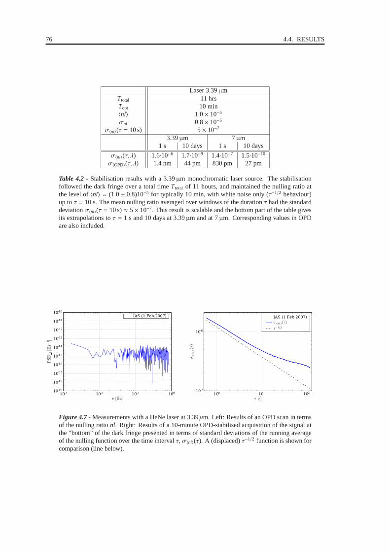
76 4.4. RESULTS
Laser 3.39µmTtotal 11 hrsTopt 10 min〈nl〉 1.0× 10⁻⁵
σnl 0.8× 10⁻⁵
σ〈nl〉(τ = 10 s) 5× 10⁻⁷
3.39µm 7µm1 s 10 days 1 s 10 days
σ〈nl〉(τ, λ) 1.6·10−6 1.7·10−9 1.4·10−7 1.5·10−10
σ〈OPD〉(τ, λ) 1.4 nm 44 pm 830 pm 27 pm
Table 4.2 - Stabilisation results with a 3.39µm monochromatic laser source. The stabilisationfollowed the dark fringe over a total timeTtotal of 11 hours, and maintained the nulling ratio atthe level of〈nl〉 = (1.0 ± 0.8)10−5 for typically 10 min, with white noise only (τ−1/2 behaviour)up toτ = 10 s. The mean nulling ratio averaged over windows of the duration τ had the standarddeviationσ〈nl〉(τ = 10 s)≈ 5× 10⁻⁷. This result is scalable and the bottom part of the table givesits extrapolations toτ = 1 s and 10 days at 3.39µm and at 7µm. Corresponding values in OPDare also included.
10-3 10-2 10-1 100
]zH[ν
10-19
10-18
10-17
10-16
10-15
10-14
10-13
10-12
10-11
10-10
l
]1− z
H[DSP
IAS (1 Feb 2007)
100 101 102
]s[τ
10-7
10-6
>ln
<)τ(
σ
IAS (1 Feb 2007)
>ln< )τ(σ
2/1−τ
Figure 4.7 - Measurements with a HeNe laser at 3.39µm. Left: Results of an OPD scan in termsof the nulling rationl. Right: Results of a 10-minute OPD-stabilised acquisitionof the signal atthe “bottom” of the dark fringe presented in terms of standard deviations of the running averageof the nulling function over the time intervalτ, σ〈nl〉(τ). A (displaced)τ−1/2 function is shown forcomparison (line below).

CHAPTER 4. STABILISATION 77
the time during which the system remained at the “bottom” of the dark fringe (best nulling-ratio values),with nl ≈ 10−5. After that drifts deteriorated nulling performance, withnl ≈ 4× 10⁻⁴.
The plot of the standard deviations of the running average ofthe nulling ratio against the width of theaveraging window (Fig.4.7, right) exposes deviations from theτ−1/2, i.e., white-noise, behaviour. The“scalable” result (analogous to Eq.4.19) is
σ〈nl〉(τ = 10 s)≈ 5× 10⁻⁷. (4.25)
Tab.4.2contains all the values derived from this.
4.5 Comparison with some other experiments
Courtesy of our colleagues (Ollivier 1999; Alcatel; Vink et al. 2003; Brachet 2005), we were able to analysetheir nulling-experiment data4. Unfortunately, in all cases, the power spectral density (PSD) of the nulloutput displays a strong peak at low frequencies, i.e., a (1/ f )α-type behaviour, withα ≥ 1 (Fig. 4.8).Consequently, none of these experiments show aτ−1/2 decrease in the standard deviation of the integratednull value, which means that the required performance cannot be obtained during very long integrations.
Let us compare our Figs.4.6 and4.7 with Fig. 4.8. It is clear that the power-spectrum density of thenulling function, PSD(nl), in the former case shows little or no 1/ f component.It must be emphasisedthat these three experiments in Fig.4.8 had the goal of achieving a low null value but not maintainingits stability. Similar conclusions can be drawn by examining the standard deviations of the mean value ofthe nulling functions over the time intervalτ, σ〈nl〉(τ). The efficiency of OPD dithering in stabilising thesetup stands out. This corresponds to an improvement of nulling stability with integration time.It mustbe stressed, however, that we start from modest nulling ratios in comparison to our colleagues,e.g., theAstrium group (Flatscher et al. 2003) reachedσ〈nl〉 ≈ 2 10−7 during 100 s.
4.6 Discussion
These results have to be regarded as preliminary because, aswe shall see in the next two Chapters, Shas not reached its designed potential so far, and the technique has not been fully tested. It is all the moreimpressive that under these conditions OPD dithering proved to be a great help in studying the performanceof our setup, providing a method of obtaining comparable results.
It is a promising method not only for laboratory use but also for space application. It does not requirededicated hardware, and represents an interesting option to setup stabilisation. A comparison with theDarwin/TPF-I requirements (Sec.2.6, Chazelas et al. 2006): 〈nl〉 = 10−5 andσ〈nl〉(10 days)= 3× 10⁻⁹
after a 10-day integration is optimistic. As shown in Tables4.2 and4.1, our K-band results extrapolate toDarwin/TPF-I conditions as
〈nl〉 (10 days, λ = 7µm) = 8× 10⁻⁹, (4.26)
our 3.39µm-laser results extrapolate as:
〈nl〉 (10 days, λ = 7µm) = 2× 10⁻¹⁰. (4.27)
It remains to be shown that the method works at the requiredDarwin/TPF-I nulling level of 10−5 inbroadband.
In the meantime, we would like to stress that we found the technique very practical in experimentalwork. We used it not only to reach and maintain the optimal OPDas we have seen, but also to perform“tweaking” experiments where the impact of small changes ininterferometer geometry, passband and othersettings on thenl and OPD can be monitored (Sec.5.2.5.1).
4This work was done at theInstitut d’astrophysique spatialewhile preparing the articleChazelas et al.(2006)

78 4.6. DISCUSSION
Figure 4.8 - Comparison with three other experiments. Left column: Power spectrum distribu-tions. Right column: Standard deviation of the running average ofnl over timeτ, σ〈nl〉(τ). Top:Results from Ollivier’s nulling experiment (Ollivier 1999; Ollivier et al. 2001). Centre: Resultsfrom the Alcatel nulling experiment (Alcatel), using a laser diode at∼ 1.57µm and an integratedoptics recombiner (courtesy Alcatel Space Industry; now Thales Alenia Space). Bottom: Astriumresults (Flatscher et al. 2003) (courtesy Astrium, Germany).

CHAPTER 4. STABILISATION 79
In our setup, we can balance the fluxes of the two interferometer arms by modifying the orientationof a folding mirror which sends both beams onto the exit fiber’s off-axis parabola. Since the beams arenot perfectly superimposed (they are parallel to within 10 arcsec but laterally shifted by about 0.1 mm),changing the point of impact on the parabola has an influence on flux mismatch. Therefore, a good exampleof a tweaking experiment consists in using OPD dithering to reach and maintain the dark fringe, and thentweak the folding mirror orientation in order to minimise the dark-fringe flux.
And finally, another practical point should be mentioned. Itis true that the next step towards fullstabilisation has to involve control of intensity mismatchbetween the interferometer arms. In order toperform tests of APS prototypes atnl = 10−5, however, OPD stabilisation suffices in providing reliable andreproducible results.

80 4.6. DISCUSSION

Chapter 5S results update
Contents5.1 Preliminaries . . . . . . . . . . . . . . . . . . . . . . . . . . . . . . . . . . . . . . . . . 82
5.1.1 Thermal and mechanical instability. . . . . . . . . . . . . . . . . . . . . . . . . 82
5.1.2 Detector calibration. . . . . . . . . . . . . . . . . . . . . . . . . . . . . . . . . . 82
5.1.3 Transmission. . . . . . . . . . . . . . . . . . . . . . . . . . . . . . . . . . . . . 82
5.2 Techniques . . . . . . . . . . . . . . . . . . . . . . . . . . . . . . . . . . . . . . . . . . 835.2.1 Zero optical path difference and the CaF2 Prisms . . . . . . . . . . . . . . . . . . 83
5.2.2 Fringe dispersion. . . . . . . . . . . . . . . . . . . . . . . . . . . . . . . . . . . 83
5.2.3 Fourier transform. . . . . . . . . . . . . . . . . . . . . . . . . . . . . . . . . . . 84
5.2.4 Direct nulling measurements. . . . . . . . . . . . . . . . . . . . . . . . . . . . . 84
5.2.5 Experimental protocol. . . . . . . . . . . . . . . . . . . . . . . . . . . . . . . . 84
5.3 Nulling levels reached withS . . . . . . . . . . . . . . . . . . . . . . . . . . . . 855.3.1 The 2000 K black body. . . . . . . . . . . . . . . . . . . . . . . . . . . . . . . . 86
5.3.2 First effective stabilisation. . . . . . . . . . . . . . . . . . . . . . . . . . . . . . 86
5.3.3 3.39µm HeNe laser and polarisers. . . . . . . . . . . . . . . . . . . . . . . . . . 86
5.3.4 S II: Improved mechanics and alignment. . . . . . . . . . . . . . . . . . . 89
5.3.5 Supercontinuum source. . . . . . . . . . . . . . . . . . . . . . . . . . . . . . . . 89
5.3.6 Focus crossing APS. . . . . . . . . . . . . . . . . . . . . . . . . . . . . . . . . 89
5.3.7 Narrow band centred at 2.3µm . . . . . . . . . . . . . . . . . . . . . . . . . . . . 90
5.3.8 Fibre curvature. . . . . . . . . . . . . . . . . . . . . . . . . . . . . . . . . . . . 90
5.3.9 L band . . . . . . . . . . . . . . . . . . . . . . . . . . . . . . . . . . . . . . . . 90
5.4 Summary . . . . . . . . . . . . . . . . . . . . . . . . . . . . . . . . . . . . . . . . . . . 91
The purpose of this Chapter is to provide an overview of the results obtained with S up to 2008.This moment in time was not chosen arbitrarily. We shall see that some of the results still remain to beinterpreted. We tried many different approaches and by mid 2008 we started running out of ideas. Atthe same time, new laboratory space was commissioned for theN testbed. In Autumn 2008, wegradually turned our attention to this new setup. This was necessary. Because of our limited manpower weare unable to operate two testbeds in parallel. What is more, we hope N brings some insights onour S results. In fact, N’s design was, in many respects, inspired by our desire to learn fromour experience with S and to decipher its puzzling performance. This is why N is a simpleroptical design with a better signal-to-noise ratio. Some indication about future N experiments willbe given in Chapter7.
The previous Chapters (3, 4) provided a description of the experimental setup, of the software systemsfor the running of the experiments, as well as of the testbed stabilisation techniques employed and the

82 5.1. PRELIMINARIES
stabilisation performance achieved. Here, we shall describe the measurement techniques developed for thetestbeds, and give an overview of the results obtained. The following Chapter (6) will provide a discussionof these results.
5.1 Preliminaries
5.1.1 Thermal and mechanical instability
We saw (Section3.3.6.1) that the issue of ambient conditions was a major concern in the design of S.Day to day experimental work validated some of the concerns and the adopted solutions while showing thatothers were to be re-evaluated.
The piezoelectric active dampening proved impractical andultimately not useful. It was difficult tooperate because it required balancing the weight on the table, carefully distributing balast. After 2005 itwas never turned on, and the piezo legs were used as a passive element only. As such, they proved veryvaluable. This was clearly shown when there was a mechanicalshort-circuit, and the granit block wasdirectly linked with the optical table. The fringe pattern became unstable.
The passive pneumatic legs under the granite block were likewise essential to the nulling performance.
Opening one of the two lids of the plexiglass case briefly and then closing it left the fringe patterndisturbed for up to 2 hours. Opening one of the small side doors was usually much less disruptive, andmeasurements without major OPD drifts were often possible within 10 minutes after the door was closed.
The thermal gradient was never imposed on the air volume in the interferometer’s housing after theinitial tests with the ceramic black body source (Section3.4.1) which did not appear to influence the nullinglevel of nl ≈ 3× 10⁻⁴ in the K band (we shall see this value very often in this Chapter). The subsequentmonochromatic measurements with the 3.39µm HeNe laser (Section3.4.2) reachednl ≈ 10−5 without theimposed thermal gradient.
The air conditioning in the laboratory is noticeably noisy.Therefore, we performed a nulling experimentwith the air conditioning off. It did not improve the nulling level in the K band beyond the very reproduciblevalue ofnl ≈ 3× 10⁻⁴.
5.1.2 Detector calibration
The InSb single-pixel detector (Section3.8.2) with the lock-in amplifier SR830 (Section3.10.1) was cali-brated (Brachet 2005, pp. 151-153). The average gain was
g ≈ 2.4× 10⁶ V/W (5.1)
which means that1 V = 420 nW. (5.2)
5.1.3 Transmission
Theoretical estimates of the transmission of the individual elements of S for the K band can be foundin Brachet(2005, pp. 127-131). We reproduce them in the left half of Table5.1.
The table also lists measured values. They are given first in the form of transmission coefficients ofindividual elements (except for the 83 % which correspond tothe transmission of two elements in series: ofthe CaF2 Prismsand the delay lines). Values for the MMZs represent one beam only. The measured powerin W is given after the input and after the output fibre.
In most cases, there is only a slight discrepancy between thetheoretical estimate and the measuredvalue. This is quite consistent with the view that the measured values must be considered to suffer from a

CHAPTER 5. SYNAPSE RESULTS UPDATE 83
theoretical transmission measured transmissionAfter per element cumulative per element cumulative
after input fibre after input fibre
input fibre 56 % 7.9 nWbeam splitter MMZ 21 % 21 % 23 % 23 %
CaF2 Prisms 88 % 18 %delay lines 92 % 17 % 83 % 19 %
beam combiner MMZ 11 % 1.9 % 10 % 1.9 %output fibre 78 % 1.5 % 45 % 0.9 %
total 0.8 % 0.7 nW
Table 5.1 - Photometry of S in the K band (Brachet 2005). Theoretical estimate and mea-sured values. These are given after each optical element (the measurement after the MMZ’scorrespond to one beam only; the 83 % after the delay lines correspond to the transmission of theCaF2 Prismsand the delay lines). The measured power in W is given after the input and afterthe output fibre. The measured values must be considered to suffer from a relative error of 10 %,while the theoretical estimate can be inaccurate as to coatings’ properties.
relative error of 10 %, and the theoretical estimate can be inaccurate as to coatings’ properties. The onlymeasured value which is clearly less than the theoretical expectation is the flux at the output of the outputfibre. This is typical of the experimental reality, however:the nulling was rarely performed with optimalcoupling at the output fibre.
5.2 Techniques
Several measurement techniques have been studied for S:
5.2.1 Zero optical path difference and the CaF2 Prisms
For each position of the CaF2 Prisms a fringe pattern can be obtained with a Long Delay Linescan. Wespoke about the theory in Section2.4, and we shall see an example in Section6.1.5.
5.2.2 Fringe dispersion
Let us briefly mention a technique studied byChazelas(2007, pp. 143-145) as well as byBoffety and Drugeon(2006). Placing an array detector with a dispersive prism at the exit of the bench while scanning the OPD,provides a series of low-resolution spectra (Fig.5.1). In an ideal case the resulting pattern would contain astraight dark fringe. Its deviation from the ideal form yields a measure of phase-shift chromaticity (Chazelas2007).
The chief advantages of this approach is that it is inherently independent of flux mismatch, and that itworks even when the signal-to-noise ratio does not allow fora direct measurement ofnl. Nonetheless, wehave not implemented this approach. One difficulty has to do with OPD drifts (which would have to bestabilised using external metrology), and the other is practical: our array detector is much more difficult touse than the single-element detector.
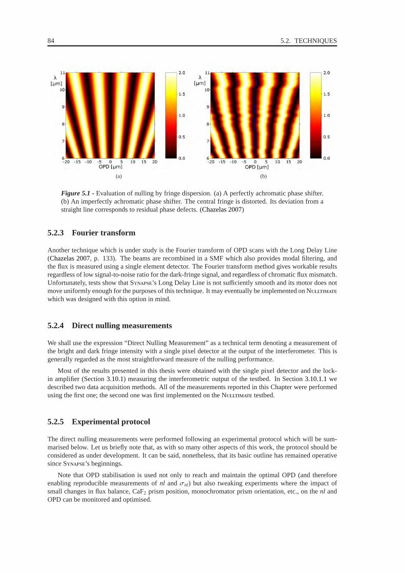
84 5.2. TECHNIQUES
(a) (b)
Figure 5.1 - Evaluation of nulling by fringe dispersion. (a) A perfectlyachromatic phase shifter.(b) An imperfectly achromatic phase shifter. The central fringe is distorted. Its deviation from astraight line corresponds to residual phase defects. (Chazelas 2007)
5.2.3 Fourier transform
Another technique which is under study is the Fourier transform of OPD scans with the Long Delay Line(Chazelas 2007, p. 133). The beams are recombined in a SMF which also provides modal filtering, andthe flux is measured using a single element detector. The Fourier transform method gives workable resultsregardless of low signal-to-noise ratio for the dark-fringe signal, and regardless of chromatic flux mismatch.Unfortunately, tests show that S’s Long Delay Line is not sufficiently smooth and its motor does notmove uniformly enough for the purposes of this technique. Itmay eventually be implemented on Nwhich was designed with this option in mind.
5.2.4 Direct nulling measurements
We shall use the expression “Direct Nulling Measurement” asa technical term denoting a measurement ofthe bright and dark fringe intensity with a single pixel detector at the output of the interferometer. This isgenerally regarded as the most straightforward measure of the nulling performance.
Most of the results presented in this thesis were obtained with the single pixel detector and the lock-in amplifier (Section3.10.1) measuring the interferometric output of the testbed. In Section 3.10.1.1wedescribed two data acquisition methods. All of the measurements reported in this Chapter were performedusing the first one; the second one was first implemented on theN testbed.
5.2.5 Experimental protocol
The direct nulling measurements were performed following an experimental protocol which will be sum-marised below. Let us briefly note that, as with so many other aspects of this work, the protocol should beconsidered as under development. It can be said, nonetheless, that its basic outline has remained operativesince S’s beginnings.
Note that OPD stabilisation is used not only to reach and maintain the optimal OPD (and thereforeenabling reproducible measurements ofnl andσnl) but also tweaking experiments where the impact ofsmall changes in flux balance, CaF2 prism position, monochromator prism orientation, etc., onthenl andOPD can be monitored and optimised.
CHAPTER 5. SYNAPSE RESULTS UPDATE 85
• Check position of optical switch: experiment with or without FC APS.
• Check CaF2 prism and long delay-line position.
• Start optimising injection into the exit fiber by maximisingBeam 1 flux with motorised folding mir-rors.
• Switch to Beam 2. Remove residual flux mismatch by tweaking folding mirror orientation (aimingfor ∆I/I ≈ 0.5%).
• Perform OPD scan with the fine delay line. Find current dark fringe position and the firstnl value.
• Repeat OPD scan, focusing on the dark fringe. Obtain a measure ofnl.
• Start OPD-stabilised DAQ, monitoring the flux and OPD position.
• Perform tweaking experiments.
5.2.5.1 Parameter tweaking experiments
A notable innovation of the protocol came with the realisation that OPD stabilisation allows for experiments(Section4.6).
• tweak folding-mirror position in order to monitor/minimise the impact of flux mismatch onnl;
• while monitoring its impact onnl, tweak CaF2 prism position in order to fine-tune the prism APS.
5.2.5.2 Flux balancing
One of the preliminary procedures in our protocol is flux balancing. We described its two elements(intensity-mismatch estimation and flux balancing) in Section 3.3.5. Here, we shall only say that patiencewas needed in order to perform the procedure successfully onS (it only rarely took less than half anhour) butwe never performed measurements unless we made sure that intensity mismatch was less than 1%,
∆II< 1 %, (5.3)
which corresponds to a nulling ratio (in the absence of all other perturbative factors; Eq.2.21):
nl < 2.5× 10⁻⁵. (5.4)
5.2.5.3 Dark current subtraction
As we have seen (Section3.10.1.2), nulling experiments often have to face the frustrating fact that the betterthe nulling performance the more likely it is to be measured with poor signal-to-noise ratio. Being close tothe sensitivity limits of the detector system leads to the natural temptation to “subtract the dark”. Indeed,when the beams are stopped, the lock-in amplifier shows a〈R〉 > 0 (Fig. 5.2). Subtracting〈R〉 from thedark-fringe signal can improve the nulling ratio as much as twofold.
We have shown (Section3.10.1.2) that this temptation must be resisted, and that the adequate procedure(unless a more careful analysis is warranted) with a well set-up measurement chain is merely to verify thatθvaries randomly when the beams are stopped.No “dark current” was subtracted from the dark-fringe flux.
5.3 Nulling levels reached withS
This Section describes the evolution of nulling measurements on the S testbed, starting in 2004.

86 5.3. NULLING LEVELS REACHED WITH SYNAPSE
5.3.1 The 2000 K black body
The first experiments with the S testbed were Simple Nulling Measurements (Section5.2.4) using asetup where:
• the source was the 2000 K ceramic black body (Section3.4.1),
• the spectral band was defined by the “K” interference filter (Section3.6),
• the bench contained only its generic achromatic phase shifter (CaF2 Prisms),
• the metrology system (Section4.2) was sometimes used for optical path difference stabilisation, and
• a thermal gradient was sometimes imposed on the air volume inside the optical bench’s protectivecase (Section3.3.6.1).
This work was performed and reported by FrankBrachet(2005). It has brought to light two featuresof the S nulling performance in the K band (2–2.5µm). The first being the best value of the nullingratio of
nl = 3× 10⁻⁴. (5.5)
The second parameter observed was the degree of nulling performance stability (cf. Chapter4). Let usreproduce the results of a typical acquisition (Fig.5.2). It is an acquisition of about 200 s with a meannulling ratio〈nl〉 = 3× 10⁻⁴ with a considerable standard deviation
σnl = 6× 10⁻⁵. (5.6)
5.3.2 First effective stabilisation
We reported about our implementation and testing of an effective OPD stabilisation system in the previousChapter (4.3). We saw that in the K band, at the nulling level of
nl = (4.7± 1.4)10−4 (5.7)
the system tracked the dark fringe for> 6 hrs, and over the whole period maintained the nulling ratioat thesame level. White noise only (τ−1/2 behaviour) was demonstrated for acquisition times up toτ = 600 s. Themean nulling ratio averaged over windows of durationτ had the standard deviation
σ〈nl〉(τ = 600 s)≈ 1.5× 10⁻⁵. (5.8)
Implementing this approach, we have succeeded not only in stabilising the nulling performance, butalso gained a powerful instrument for bench optimisation (cf. Sec.5.2).
5.3.3 3.39µm HeNe laser and polarisers
In order to find ways of improving the nulling performance of the testbed, we started working with monochro-matic light, at 3.39µm, produced by a HeNe laser (Section3.4.2). The first results were limited to
⟨
nlunpolarised
⟩
= 6× 10⁻⁵. (5.9)
Introducing polarisers has led to⟨
nlpolarised
⟩
= 10−5. (5.10)
An OPD scan is shown in Fig.5.3. This result seems roughly consistent with our theoreticalstudies(Chazelas 2007) of the effects of polarisation mismatch (primarily due to residual alignment errors) onthe nulling performance. Let us mention that this apparent accord with the theoretical model will have tobe discussed in more detail in the following Chapter (6). We felt justified, however, in wanting to re-alignour optics carefully. In fact, we found that this was only possible if some improvements were made to themechanics of the testbed. The upgraded setup became known asS II.

CHAPTER 5. SYNAPSE RESULTS UPDATE 87
Figure 5.2 - Smeasurements of recombined flux in the K spectral band, normalised divid-ing by the mean bright fringe flux. The transition between thebright fringe (the first 50 seconds)and the dark fringe (between 50 s and 240 s) was performed manually by modifying the length ofthe delay line. The last part of the curve shows the lock-in amplifier’s module outputR when thedetector was covered, illustrating that measurement chainwas well set up.

88 5.3. NULLING LEVELS REACHED WITH SYNAPSE
4 5 6 7 8 9 10 11]mµ[dpo
10-5
10-4
10-3
10-2
10-1
100
ln
Figure 5.3 - Measurements with a HeNe laser at 3.39µm. Results of an OPD scan in terms of thenulling rationl. The fact that the fringes do not seem to be of equal depth is attributable to thescan’s step (10 nm; which is too coarse).

CHAPTER 5. SYNAPSE RESULTS UPDATE 89
polarisersλ without with
K band 5× 10⁻⁴ 3× 10⁻⁴
3.39µm 5× 10⁻⁵ 1× 10⁻⁵
Table 5.2 - Nulling performance of S II.
5.3.4 S II : Improved mechanics and alignment
After these encouraging results with monochromatic light we concentrated our efforts on improving thelevel of null in broad band. From the results of monochromatic measurements we deduced that the factorlimiting nulling levels of the test bench could not be thermal and mechanical (vibrations) stability. Suchphenomena would also deteriorate monochromatic nulling performance.
We have also seen that improving bench alignment (to within< 10 arcsec as opposed to the previous< 3 arcmin) may help reduce polarisation mismatch, greatly facilitating flux balancing of the two inter-ferometer arms. Performing direct nulling measurements with and without polarisers in this improvedsetup has demonstrated a surprising consistency with the results obtained with the first version of S(Tab.5.2).
As we have seen in the previous Chapter (4.4.2), OPD-stabilised long-duration measurements (the OPDdithering was able to track the dark fringe over a period> 11 hrs, maintaining the nulling ratio at the levelof
〈nl〉 = (1.0± 0.8) 10−5 (5.11)
for typically 10 min, with white noise only (τ−1/2 behaviour) up toτ = 10 s. The mean nulling ratioaveraged over windows of the durationτ had the standard deviation
σ〈nl〉(τ = 10 s)≈ 5× 10⁻⁷ (5.12)
Conclusion. From these measurements we had to conclude that improving the alignment, although veryuseful as regards practical aspects of experimental work,did not alter overall nulling performance.
5.3.5 Supercontinuum source
The previous measurements, especially those taken with thepolarisers, had a relatively small signal-to-noise ratio. The noise can be quantified as, typically,σN = 0.5µV whereas the dark fringe fluxes weretypically a fewµV.
In order to improve the situation, as well as to gain new experimental possibilities (we shall see one inSection5.3.7), we upgraded our setup and acquired a supercontinuum source (Section3.4.3). It providesa usable flux of about 200 mW in the K band (about a million timesmore than 0.17µW, which is the fluxavailable from the ceramic black body).
Even with this new light source, the nulling performance didnot improve, and remained at the previ-ously reported levels.
5.3.6 Focus crossing APS
S II was also designed to permit measurements of the Focus Crossing (or Through Focus) APSprototype (Section3.9.1). It was initially built to work in the spectral range of 6–18µm (proposed rangefor Darwin/TPF-I), and its optimal designed nulling performance is
nlFC APS(optimal)≤ 10−6, (5.13)

90 5.3. NULLING LEVELS REACHED WITH SYNAPSE
λ with polarisers
K band 3× 10⁻⁴
3.39µm 1× 10⁻⁵
Table 5.3 - Nulling performance of S II with the Focus Crossing APS prototype.
without withλ FC APS
narrow band 3.4× 10⁻⁴ 3.4× 10⁻⁴
Table 5.4 - Nulling performance of S II with the narrow passband filter (16 nm FWHM)centred around 2.3µm.
depending on the bench configuration. In the working conditions of S the expected value is
nlFC APS(expected)≤ 10−5. (5.14)
Using the CaF2 Prisms as chromatism compensators (Section3.3.7), we tested the FC APS prototypewith polarisers. Both in the K band and with the monochromatic 3.39µm laser we once again obtained thesame values (Tab.5.3) as without the FC APS prototype and the CaF2 Prisms used as an APS.
Conclusion. The expected performance (nl = 10−5) was demonstrated with laser light at 3.39µm. Rejec-tion performance of the FC APS in the K band (2.0–2.5µm) was limited by the performance of the SII testbed itself.
5.3.7 Narrow band centred at2.3µm
The high flux of the supercontinuum source in conjunction with an interferometric filter with a narrowpassband (16 nm FWHM) centred around 2.3µm, enabled us to perform a number of decisive experiments(we shall discuss their implications in the following Chapter 6). The results are summarised in Tab.5.4.
5.3.8 Fibre curvature
In order to explore the possibility that S nulling performance is limited in non-monochromatic lightby the quality of modal filtering, we performed tests with oursingle-mode fibres. Twisting the fibre arounda 40 mm diametre cylinder (3 or 8 full turns) was suggested as ameans for improving secondary-moderejection.
These direct nulling measurements were performed in the K band (2.0–2.4µm) with the polarisers butwithout the FC APS. The measured nulling ratio
nl = 1.9× 10⁻⁴ (5.15)
demonstrated some improvement. No reproducible difference was observed between setups with 3 and 8full turns of the fibre.
5.3.9 L band
One of our experiments to explore the possibility that S nulling performance is limited in non-monochromatic light by our modal filters was performed in theL band (3–4µm). The setup was otherwise

CHAPTER 5. SYNAPSE RESULTS UPDATE 91
unchanged. Although we have L-band single-mode fibres, in this case we used the ones designed for the Kband, i.e., with a cutoff wavelength ofλc = 1.95µm. Taking fibres designed for the K band and using themin the L band reduces the throughput but may improve modal filtering properties.
These direct nulling measurements were thus performed in the L band (3–4µm) with the polarisers butwithout the FC APS. The measured nulling ratio
nl = 2.1× 10⁻⁴ (5.16)
again indicated some improvement. This value was obtained with a poor signal-to-noise ratio, however, andshould be regarded as an upper limit.
5.4 Summary
An overview of our progress in terms ofnl and stability (when available) is given in Tab.5.5. Three pointsstand out:
1. Focus-Crossing APS prototype’s nulling ability was validated with the 3.39µm laser to the level of10−5. The performance of the setup in the K band was not limited by the prototype.
2. Polarisation. The presence of polarisers clearly improves the nulling ratio. In all configurations wherewe tested the nulling performance with and without polarisers, the setup with polarisers provides betternulling ratios. We shall see (Sec.6.1.3) that this effect is not fully explained by the available theoreticalmodels.
3. Particularity of 3.39µm-laser light? What stands out is a discrepancy between the nulling ratiosachieved with the 3.39µm laser source and with all other tested configurations. If itwere an issue ofchromatism, we would expect to see a difference between K-band results and the results obtained withthenarrow (16 nm FWHM) filter at 2.3µm (Sec.5.3.7). Perhaps it is an issue of the Single-Mode Fibres. Thelast two tests, viz., twisting the SMF (Sec.5.3.8) and using the K-band SMF in the L band (Sec.5.3.9),seem to suggest that this may be the case.
The last two issues will be discussed more closely in the nextChapter (6).

92 5.4. SUMMARY
λ polarisers APS FC nl stability
Nov ’05 K band – – 3× 10⁻⁴
May ’06 K band – – 5× 10⁻⁴ σ〈nl〉(600 s)= 1.5× 10⁻⁵
Jan ’07 3.39µm – – 10−4
Jan ’07 3.39µm + – 6× 10⁻⁵ σ〈nl〉(10 s)= 5× 10⁻⁷
Feb ’08 3.39µm + – 10−5
Feb ’08 3.39µm + + 10−5
Feb ’08 K band – + 4× 10⁻⁴
Feb ’08 K band + + 4× 10⁻⁴
May ’08 2.3µm (16 nm FWHM) + – 3.4× 10⁻⁴
May ’08 K band (SMF twist) + – 1.9× 10⁻⁴
Jun ’08 L band (K-band SMF) + – < 2.1× 10⁻⁴
Table 5.5 - An overview of progress on S in terms ofnl and stability (when available)expressed in terms of the standard deviation of the nulling-ratio means averaged over windows ofthe durationτ, σ〈nl〉(τ) (these values are scalable asτ−1/2 because there is white noise only).

Chapter 6Error budget
Contents6.1 Tests and models. . . . . . . . . . . . . . . . . . . . . . . . . . . . . . . . . . . . . . . 93
6.1.1 Detector nonlinearity. . . . . . . . . . . . . . . . . . . . . . . . . . . . . . . . . 93
6.1.2 Beam path . . . . . . . . . . . . . . . . . . . . . . . . . . . . . . . . . . . . . . 94
6.1.3 Polarisation. . . . . . . . . . . . . . . . . . . . . . . . . . . . . . . . . . . . . . 94
6.1.4 Chromatic shear and other dispersive effects. . . . . . . . . . . . . . . . . . . . . 96
6.1.5 CaF2 Prisms: multiple working points. . . . . . . . . . . . . . . . . . . . . . . . 98
6.1.6 Coatings . . . . . . . . . . . . . . . . . . . . . . . . . . . . . . . . . . . . . . . 99
6.1.7 Inhomogeneities. . . . . . . . . . . . . . . . . . . . . . . . . . . . . . . . . . . 99
6.1.8 Spectral mismatch. . . . . . . . . . . . . . . . . . . . . . . . . . . . . . . . . . 101
6.1.9 Wavefront quality. . . . . . . . . . . . . . . . . . . . . . . . . . . . . . . . . . . 101
6.2 Testing onN . . . . . . . . . . . . . . . . . . . . . . . . . . . . . . . . . . . . 102
6.3 Error budget . . . . . . . . . . . . . . . . . . . . . . . . . . . . . . . . . . . . . . . . . 102
6.4 Summary . . . . . . . . . . . . . . . . . . . . . . . . . . . . . . . . . . . . . . . . . . . 104
The purpose of this Chapter will be twofold: (1) to discuss the setup’s error budget and thereforethe expected performance levels, and (2) to list and describe all the avenues we explored while tryingto understand our results. As we have seen in the previous Chapter (5), some of results we obtained sofar on S II, must be regarded as preliminary until we reach a full understanding of the underlyingphenomena. The two observations that require special attention are
1. polarisation: there seems to be a discrepancy between thetheoretical predictions and our observa-tions;
2. why are the nulling ratios achieved with the 3.39µm-laser light better than those obtained in otherconfigurations?
6.1 Tests and models
6.1.1 Detector nonlinearity
The accuracy of nulling measurements depends on the detection system’s linearity. The nulling ratio iscalculated from two measurements: of the bright fringe, andof the dark fringe. Since the whole purpose of

94 6.1. TESTS AND MODELS
nulling experiments is that these two measurements differ by several orders of magnitude, it is clear that thedetection system must have a linear response curve (as a function of flux intensity).
The PhD thesis of ChristopheBuisset(2007) contains a detailed study of the response curve of a de-tection system very similar to our own, comprising a single pixel detector (InGaAs) and a lock-in amplifier(Stanford Research 830). He used two polarisers to modulatethe measured intensity over six orders ofmagnitude. He concluded that the non-linearity of the detection system induces an inaccuracy of less than7 % in the nulling ratio.
After a discussion with Christophe’s director, Yves Rabbia, we decided to try a different approach, inorder to obtain an independent estimate ourselves, but mainly to confirm that our detection system doesnot significantly deviate from linearity. While we use the same lock-in amplifier model, our single pixeldetector is not identical to the type Christophe used (ours is InSb, produced byElectro-Optical Systems).
We demonstrated (App.D) that our detector system is linear within an error of≈ 10%. The methodwe applied is not sensitive enough to provide a better constraint, probably because of the geometric factorclose to the detector. A better approximation of a point source would be advisable.
Conclusion. A non-linearity within the measured limits (≈ 10 %) does not explain our observations.
6.1.2 Beam path
We have already mentioned (Section3.12) that the better quality of the mechanics and of the alignmentin S II clearly improved the setup in terms of solidness and reproducibility of measurements. Re-aligning the bench and the measurements performed on the occasion, also allowed us to eliminate certainhypotheses that, if true, might have offered insights into our results:
• vignetting,
• mismatched and/or non-Gaussian beam profiles.
We verified whether there were any obstructions in the optical path in the visible with cameras, takingpictures of the beam, and in the infrared with pinhole scans (Fig. 6.1).
Conclusion. The measured beam profiles were consistent with the Gaussianspatial distribution. We thusverified that neither vignetting nor other beam profile mismatch is a factor in our setup.
6.1.3 Polarisation
Our colleagues in Nice (Weber 2004; Buisset 2007), as well as BrunoChazelas(2007) studied the issue.
Bruno Chazelas(2007) concludes that if all the surfaces of S are aligned with a tolerance of±46 arcsec, the nulling ratio in the K band should be better than 10−6. At the wavelength of 3.39µm, thealignment tolerance necessary fornl < 10−6 is slightly less stringent, viz.,±43 arcsec.
Conclusion. The improved alignment of S II is within ±10 arcsec. The fact that nulling-ratiomeasurements in monochromatic light without polarisers were five times worse than with polarisers seemsto indicate that the theoretical models do not account for the observed results.

CHAPTER 6. ERROR BUDGET 95
Figure 6.1 - Beam profiles obtained with pinhole (1.5 mm) scans in the infrared. The scans onthe left represent beam 1, those on the right, beam 2. The scans on top were performed vertically,those on bottom, horizontally. Error of each point≈ 0.2 %.
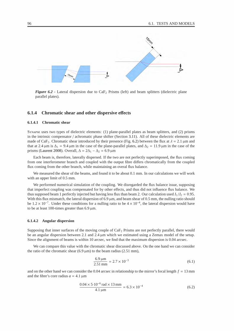
96 6.1. TESTS AND MODELS
Figure 6.2 - Lateral dispersion due to CaF2 Prisms (left) and beam splitters (dielectric planeparallel plates).
6.1.4 Chromatic shear and other dispersive effects
6.1.4.1 Chromatic shear
S uses two types of dielectric elements: (1) plane-parallel plates as beam splitters, and (2) prismsin the intrinsic compensator/ achromatic phase shifter (Section3.11). All of these dielectric elements aremade of CaF2. Chromatic shear introduced by their presence (Fig.6.2) between the flux atλ = 2.1µm andthat at 2.4µm is∆1 = 9.4µm in the case of the plane-parallel plates, and∆2 = 11.9µm in the case of theprisms (Laurent 2008). Overall,∆ = 2∆1 − ∆2 = 6.9µm
Each beam is, therefore, laterally dispersed. If the two arenot perfectly superimposed, the flux comingfrom one interferometer branch and coupled with the output fibre differs chromatically from the coupledflux coming from the other branch, while maintaining an overal flux balance.
We measured the shear of the beams, and found it to be about 0.1mm. In our calculations we will workwith an upper limit of 0.5 mm.
We performed numerical simulation of the coupling. We disregarded the flux balance issue, supposingthat imperfect coupling was compensated for by other effects, and thus did not influence flux balance. Wethus supposed beam 1 perfectly injected but having less flux than beam 2. Our calculation usedI1/I2 = 0.95.With this flux mismatch, the lateral dispersion of 6.9µm, and beam shear of 0.5 mm, the nulling ratio shouldbe 1.2× 10⁻⁷. Under these conditions for a nulling ratio to be 4× 10⁻⁴, the lateral dispersion would haveto be at least 100-times greater than 6.9µm.
6.1.4.2 Angular dispersion
Supposing that inner surfaces of the moving couple of CaF2 Prisms are not perfectly parallel, there wouldbe an angular dispersion between 2.1 and 2.4µm which we estimated using a Zemax model of the setup.Since the alignment of beams is within 10 arcsec, we find that the maximum dispersion is 0.04 arcsec.
We can compare this value with the chromatic shear discussedabove. On the one hand we can considerthe ratio of the chromatic shear (6.9µm) to the beam radius (2.51 mm),
6.9µm2.51 mm
= 2.7× 10⁻³ (6.1)
and on the other hand we can consider the 0.04 arcsec in relationship to the mirror’s focal lengthf = 13 mmand the fibre’s core radiusa = 4.1µm
0.04× 5·10−6 rad× 13 mm4.1µm
= 6.3× 10⁻⁴ (6.2)

CHAPTER 6. ERROR BUDGET 97
Figure 6.3 - Verification of the equality of air colums between the two pairs of CaF2 Prisms. Thefixed pair’s separation is 15 mm.
Therefore, the angular dispersion is even less of a problem than the worst-case chromatic-shear scenario.
6.1.4.3 Unequal air columns in CaF2 Prisms
Another possible chromatic effect arises from unequal air colums between the two pairs of CaF2 Prisms.These values were verified to be equal to within 0.1 mm (Fig.6.3). Calculations show that if the differenceis 0.1 (worst case), then the expected nulling ratio should be
nl = 5× 10⁻⁶, (6.3)
again integrating betweenλmin = 2.1µm andλmax = 2.4µm.
6.1.4.4 Off-axis parabola defects
Supposing that the two beams impact two distinct regions of the injection off-axis parabola in front of theoutput fibre, further supposing that in one of these regions the parabolic mirror would be perfect whereasthe other one would have severe defects, the effects on two beams would be that they would become outof phase, and that their coupling with the output fibre would be unequal, i.e., there would be an intensitymismatch. The phase defect would not be an issue because it would be corrected by the delay lines. Theflux mismatch, however, needs to be considered a little more closely.
In our worst-case-scenario model, the defects of the off-axis parabola are causing a flux mismatchwhich is fully compensated for by other means (e.g., knife edges). In our calculations we consider twomonochromatic beams, one at 2.125µm, and the other at 2.325µm. We find that in order to limitnl =3× 10⁻⁴, the surface of the parabolas would have to be atλv/5 RMS orλv/1.7 PTV (if the relationshipbetween RMS and PTV is as in the sinusoidal case). These numbers appear less than an order of magnitudegreater than what we would expect from manufacturer’s specifications. Let us look at the flux mismatchthat would have to be compensated for by the aforementioned “other means”. It turns out to be 36 %. Thiscannot be the case because there simply are no knife edges in the beam path.

98 6.1. TESTS AND MODELS
Figure 6.4 - Injection shear. The axis of the fibre intersects the Off-Axis Parabola (OAP; rep-resented here as a convex lens) at a certain point. The axis ofthe beam intersects the OAP at adifferent point. The distance between these two points is the injection shear,δ. It corresponds tothe angleα = δ/r, wherer = 2 f /(1+ cosθ), f being the focal length of the OAP, andθ its angle(Sec.3.3.3).
6.1.4.5 Narrow passband filter
After careful study of the chromatic shear and other dispersive effects (which lasted a couple of months)we found that none of them can account for our observed K-bandnulling ratio. What is more, we thendiscovered that we had a narrow passband interferometric filter (Sec.3.6), centred around 2.3µm and witha FWHM of only 16 nm. Reducing the passband fromλ/∆λ of 7.5 (the values we used in our calculationswere 2.1 and 2.4µm) to 150, i.e., by a factor of 20, typically reduces the expected chromatic effects by thesame factor. As was reported in the previous Chapter (5.3.7), the measurements with the narrow passbandfilter yielded approximately the same nulling ratios as withthe K band filter (3.4× 10⁻⁴ and 4× 10⁻⁴
respectively).
Conclusion. These chromatic effects do not explain the measured nulling ratios. S is not limitedby the chromatic shear, and other considered dispersive phenomena.
6.1.5 CaF2 Prisms: multiple working points
When searching for the working point of S, there are two parameters that need to be tuned: thedifferential thicknesse of the dielectric represented our CaF2 Prisms, and the optical-path difference OPDrealised by our delay lines (Sec.2.4). It could be that we did not choose the optimal working pointin thistwo-dimensional parameter space. OPD scans may show similar fringe patterns corresponding to phaseshifts of (2n− 1)π, but the optimal (in terms of providing the best nulling performance) working position isunique. With a degraded null it is possible to mistakea working point fortheworking point.
We verified this by a series of measurements shown in Fig.6.6, examining nulling ratios at working

CHAPTER 6. ERROR BUDGET 99
Figure 6.5 - Injection tip/tilt. The proper mode of the fibre is collimated by the Off-Axis Parabola(OAP; represented here as a convex lens). The axis of this putative collimated beam is shown bythe dotted line. It is at an angleβ to the incident beam. This means that the beam does not impactthe fibrehead at its centre but at a point which is at the distance∆ from the centre of the fibre.
points ranging from−11π to +11π.
Conclusion. We verfied that the interferometer was at the optimal workingpoint in the two-dimensionalspace defined by the parameters of OPD and differential dielectric thickness.
6.1.6 Coatings
S beam splitters bare coatings (Sec.3.11). If these coatings were unequal, there could be a chromaticdifference between the two arms of the interferometer.
Using McLeod software, we simulated a 10 % difference in the thickness of our coatings, and obtained
nl < 10−6 (6.4)
Conclusion. Simulations suggest that differences in thickness between beam splitters cannot limit thetestbed’s nulling ability to the observed degree.
6.1.7 Inhomogeneities
Similarly, the dielectric substrate of the beam splitters and of the prisms was checked interferometrically forinhomogeneities by our optics supplier when they started working with it. The material was homogeneousto a degree which would enable us to measure
nl < 10−6 (6.5)

100 6.1. TESTS AND MODELS
Figure 6.6 - Nulling measurement at different CaF2 working points. Crosses represent a seriesof measurements, ranging from−11π to +11π. Stars are another series of measurements, thedifference between the first and second series being an indicatorof the measurement’s uncertainty.The full line is an parabolic fit of the data (first series of measurements only). The circles and thedotted line represent the theoretical model.

CHAPTER 6. ERROR BUDGET 101
Figure 6.7 - Verification of the spectral mismatch between the two beams.Two measurementsper beam were made. “v1” and “v2” designate the two beams. (Intensity in arbitrary units vs.wavelength in nm. )
Conclusion. The homogeneity of the CaF2 used in our optics should allow S to reach nulling levelsthat we have not observed.
6.1.8 Spectral mismatch
If the two beams were not perfectly matched spectrally, the nulling ratio would suffer. Therefore, we per-formed a series of spectral measurements of the light emitted at the exit of the output fibre. The spectrometerhad 256 channels between 858.68 and 2595.46 nm. It operated at -10 C (with a Pelletier system). We mea-sured each beam twice. Each of the four measurements comprised 50 scans, each scan being an average of10 integration periods of 10 ms.
The results are presented in Fig.6.7. The differences between the two beams are of the same order asthe differences between the individual measurements of each beam. This is consistent with the hypothesisthat the observed differences between the two beams are due to measurement noise.
We calculated the nulling ratio corresponding to the situation when the observed spectral differenceswould be only due to real spectral mismatch between the two beams (worst-case scenario). Our estimate is
nl = 3.8× 10⁻⁵. (6.6)
Conclusion. Even if the measured spectral variations were dominated by areal spectral mismatch betweenthe two arms of the interferometer, the corresponding nulling ratios are an order of magnitude better thanthe observed values in the K band.
6.1.9 Wavefront quality
We recalled the importance of wavefront quality in nulling interferometry, and the influence of modalfiltering with single-mode fibres (Section2.5). As reported in Sections5.3.8and5.3.9we performed someexperiments aimed at improving secondary-mode rejection.They were performed with relatively low levelsof flux, and their results cannot be regarded as fully reliable. They do, nonetheless, seem to indicate thatmore study is needed on the performance of our SMFs.
The last experiments performed on S II (July 2008) before we concentrated on N aimedat determining the quality of the injection into the fibres.

102 6.2. TESTING ON NULLTIMATE
Since we could not easily examine the output fibre, we decidedto perform a series of experiments on theinput fibre. In the previous experiments, the 3.39µm-laser beam was focused on the fibrehead with an OAP( f = 13 mm,α = 35), whereas the supercontinuum source used a dedicated setupto couple its photonic-crystal fibre with the testbed’s input SMF. For the new experiments we modified our injection system inthe case of the supercontinuum source. With another OAP, we generated a collimated beam which we theninjected into the testbed’s input SMF via the same OAP that the laser used. Now, both sources were injectedinto the testbed’s input fibre via the same OAP (f = 13 mm,α = 35). We performed nulling measurementswith both sources, obtaining
nl = 10−5 with 3.39µm laser, (6.7)
nl = 4× 10⁻⁴ with supercontinuum. (6.8)
We also performed scans of the optical field at the injection point by translating the fibrehead vertically. Wefound roughly Gaussian distributions with
FWHM = 37µm with 3.39µm laser, (6.9)
FWHM = 12µm with supercontinuum. (6.10)
This result was unexpected. We hoped to find the exact opposite. In that case we would have concludedthat indeed there is a problem with cladding modes in the caseof the supercontinuum source. What wefound did not allow us to draw any conclusions. Does the FWHM= 37µm in the case of the laser meanthat we are injecting some flux in the cladding? It is possiblethat it does not limit the nulling ratio becausethe laser beam is monochromatic and highly coherent. On the other hand, the supercontinuum beam alsoshould be coherent, and while its FWHM is three times smaller,it is still about twice as large as the SMF’sacceptance lobe.
Once again we realised that we faced a dilemma: Either perform careful diagnostics on our equipment,or procede without delay towards our objectives (in this case APS prototype testing, and the commission-ing of N). We opted for the latter, hoping that N will either provide a good nullingperformance, or allow us to conduct better tests, mainly thanks to the higher level of flux.
6.2 Testing onN
As we have concluded in the previous Section (6.1.9), we chose to abandon the tests on S andconcentrate on N. We have worked hard to achieve very high levels of flux with N, andthe preliminary measurements seem to indicate that we will be able to work with fluxes that were beyondour reach with S (perhaps by a factor 103). This is important because some of the experiments weare planning to perform are impossible without good flux. Theplanned experiments include:
• Monochromatic and narrow passband: compare high signal-to-noise (SNR) nulling ratios obtainedwith the 2.32µm laser diode and with the 16 nm FWHM narrow passband filter;
• 2.32µm and 3.39µm laser sources: compare high SNR nulling ratios obtained with two trulymonochromatic sources, emitting at different wavelengths, both within the SMF’s interval betweenits cutoff wavelengthλco and 2λco;
• Polarisation: perform high SNR nulling experiments in polarised light, i.e., obtain a reproduciblenulling ratio with thes andp polarisations (as defined by the 45 incidence on most of our optics).
6.3 Error budget
FollowingSerabyn(2000), it has become customary to list the contributors that degrade the null (Buisset et al.2007; Gappinger et al. 2009) in an overview, summing the individual terms. We shall endeavour to providea similar error budget in Table6.1, bringing together the elements already discussed in the previous pages.
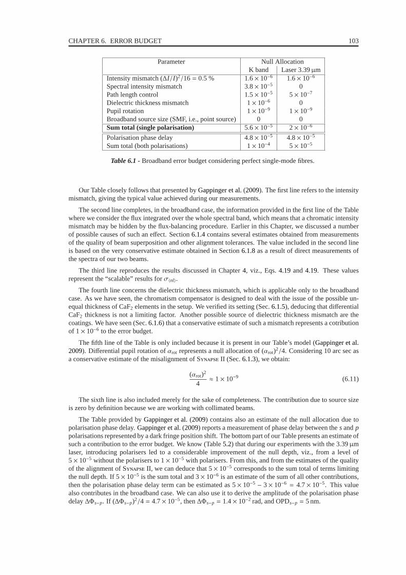
CHAPTER 6. ERROR BUDGET 103
Parameter Null AllocationK band Laser 3.39µm
Intensity mismatch (∆I/I )2/16= 0.5 % 1.6× 10⁻⁶ 1.6× 10⁻⁶
Spectral intensity mismatch 3.8× 10⁻⁵ 0Path length control 1.5× 10⁻⁵ 5× 10⁻⁷
Dielectric thickness mismatch 1× 10⁻⁶ 0Pupil rotation 1× 10⁻⁹ 1× 10⁻⁹
Broadband source size (SMF, i.e., point source) 0 0Sum total (single polarisation) 5.6× 10⁻⁵ 2× 10⁻⁶
Polarisation phase delay 4.8× 10⁻⁵ 4.8× 10⁻⁵
Sum total (both polarisations) 1× 10⁻⁴ 5× 10⁻⁵
Table 6.1 - Broadband error budget considering perfect single-mode fibres.
Our Table closely follows that presented byGappinger et al.(2009). The first line refers to the intensitymismatch, giving the typical value achieved during our measurements.
The second line completes, in the broadband case, the information provided in the first line of the Tablewhere we consider the flux integrated over the whole spectralband, which means that a chromatic intensitymismatch may be hidden by the flux-balancing procedure. Earlier in this Chapter, we discussed a numberof possible causes of such an effect. Section6.1.4contains several estimates obtained from measurementsof the quality of beam superposition and other alignment tolerances. The value included in the second lineis based on the very conservative estimate obtained in Section 6.1.8as a result of direct measurements ofthe spectra of our two beams.
The third line reproduces the results discussed in Chapter4, viz., Eqs.4.19 and4.19. These valuesrepresent the “scalable” results forσ〈nl〉.
The fourth line concerns the dielectric thickness mismatch, which is applicable only to the broadbandcase. As we have seen, the chromatism compensator is designed to deal with the issue of the possible un-equal thickness of CaF2 elements in the setup. We verified its setting (Sec.6.1.5), deducing that differentialCaF2 thickness is not a limiting factor. Another possible sourceof dielectric thickness mismatch are thecoatings. We have seen (Sec.6.1.6) that a conservative estimate of such a mismatch representsa cotributionof 1× 10⁻⁶ to the error budget.
The fifth line of the Table is only included because it is present in our Table’s model (Gappinger et al.2009). Differential pupil rotation ofαrot represents a null allocation of (αrot)2/4. Considering 10 arc sec asa conservative estimate of the misalignment of S II (Sec.6.1.3), we obtain:
(αrot)2
4≈ 1× 10⁻⁹ (6.11)
The sixth line is also included merely for the sake of completeness. The contribution due to source sizeis zero by definition because we are working with collimated beams.
The Table provided byGappinger et al.(2009) contains also an estimate of the null allocation due topolarisation phase delay.Gappinger et al.(2009) reports a measurement of phase delay between thesandppolarisations represented by a dark fringe position shift.The bottom part of our Table presents an estimate ofsuch a contribution to the error budget. We know (Table5.2) that during our experiments with the 3.39µmlaser, introducing polarisers led to a considerable improvement of the null depth, viz., from a level of5× 10−5 without the polarisers to 1× 10⁻⁵ with polarisers. From this, and from the estimates of the qualityof the alignment of S II, we can deduce that 5× 10⁻⁵ corresponds to the sum total of terms limitingthe null depth. If 5× 10⁻⁵ is the sum total and 3× 10⁻⁶ is an estimate of the sum of all other contributions,then the polarisation phase delay term can be estimated as 5× 10⁻⁵ − 3× 10−6 = 4.7× 10⁻⁵. This valuealso contributes in the broadband case. We can also use it to derive the amplitude of the polarisation phasedelay∆Φs−p. If (∆Φs−p)2/4 = 4.7× 10⁻⁵, then∆Φs−p = 1.4× 10⁻² rad, and OPDs−p = 5 nm.

104 6.4. SUMMARY
A similar reasoning can lead us to an estimate of the contribution of the single-mode fibres to the errorbudget. If we consider the broadband null depth of 3× 10⁻⁴ (with polarisers), and the estimated sum totalof all other contributions to the error budget which we find tobe 5.6× 10⁻⁵ in the K band (with polarisers),we can deduce that the single-mode fibres contribute 2.4× 10⁻⁴ to the error budget in the K band (withpolarisers). This would mean that they reject incoherent light at a ratio of 4000:1.
6.4 Summary
We examined a large spectrum of phenomena that could affect S’s broadband nulling performance.Theoretical models preclude a certain number of them from being considered as the possible cause. Otherswere eliminated by experimental results (e.g.,nl = 3.4× 10⁻⁴ with the 16 nm FWHM passband filter). Wedecided to suspend this effort, and concentrate our forces on the preparation of a new experimental setup,the N testbed.

Chapter 7Conclusions and perspectives
Contents7.1 What was to be done. . . . . . . . . . . . . . . . . . . . . . . . . . . . . . . . . . . . . 1057.2 What was done. . . . . . . . . . . . . . . . . . . . . . . . . . . . . . . . . . . . . . . . 106
7.2.1 My contribution . . . . . . . . . . . . . . . . . . . . . . . . . . . . . . . . . . . 106
7.3 Perspectives . . . . . . . . . . . . . . . . . . . . . . . . . . . . . . . . . . . . . . . . . 1077.3.1 N . . . . . . . . . . . . . . . . . . . . . . . . . . . . . . . . . . . . . . 107
7.3.2 Polarisation. . . . . . . . . . . . . . . . . . . . . . . . . . . . . . . . . . . . . . 107
7.3.3 Tests of achromatic phase shifters. . . . . . . . . . . . . . . . . . . . . . . . . . 107
7.3.4 Flux-balance stabilisation. . . . . . . . . . . . . . . . . . . . . . . . . . . . . . 108
7.3.5 Experiments around 10µm . . . . . . . . . . . . . . . . . . . . . . . . . . . . . . 108
7.4 Towards a flagship space mission. . . . . . . . . . . . . . . . . . . . . . . . . . . . . . 1087.5 Summary . . . . . . . . . . . . . . . . . . . . . . . . . . . . . . . . . . . . . . . . . . . 109
We shall first recall the goals of our team’s work, we shall present a brief summary of what was achieved,enumerating my personal contributions, then we shall indicate some of the future work, and finally we shallsituate our endeavours in the context of the preparation of aspaceborne nulling interferometer like theDarwin/TPF-I space mission.
7.1 What was to be done
In the Preface we outlined the science goals of our work, listing four points:
• stabilising the S tested,
• improving the performance of the S testbed,
• building the N testbed as its successor,
• testing the achromatic phase shifter prototypes.
Let us recall that by the end of its commissioning, in late 2005, it was clear that the S testbedwas suffering from drifts and that its performance in terms of the nulling ratio was limited to a level whichwas a factor 300 less than the designed value. The drifts madeit difficult to perform reliable diagnostics onthe testbed, and therefore the first order of business was to find an efficient way of conducting reproduciblemeasurements.

106 7.2. WHAT WAS DONE
The second goal was then to see what could be done to improve the performance and bring it up to theexpected levels, identifying the causes of the unexpectedly large broadband nulling ratio.
The third goal was to build another testbed, N. The original purpose of the project was similarto that of the S testbed, viz., achromatic phase shifter prototype testing. Unlike S, the newbench was to be cryogenic and, ideally, work in the band 6–18µm. By the time I joined the team at theInstitut d’Astrophysique Spatialeit was clear that N could be cryogenic only if we understood whythere was a problem with S.
The fourth goal, often presented (to the funding agencies) as the only one, was to test the prototypes ofachromatic phase shifters constructed by our colleagues inNice, Cannes, Heidelberg, and Liege. By theend of my first year, the latter (Liege) was dropped, and its testing was to be done elsewhere.
7.2 What was done
The first goal was achieved quite satisfactorily by implementing an optical-path difference stabilisationalgorithm (OPD dithering; Chap.4). In addition to it being an interesting technique that may prove usefuleven in the context of a space mission, it is thanks to this system that we were able to conduct reproduciblemeasurements of S’s nulling performance.
We found that the 3× 10⁻⁴ nulling ratio minimum was not due to OPD drifts. In order to study the originof this limit we tested the stability of Swith the 3.39µm laser, finding a surprising improvement of thenulling performance especially once we started working with polarised light. This indicated that the testbedwas poorly aligned. We decided to undertake a major overhaulof the mechanics and a new alignment of thetestbed. New electronics were installed and new software was developed. The improved testbed, SII, aimed at the second goal listed above. The new setup did not solve the problem of the 3× 10⁻⁴ nullinglevels broadband, and a series of tests were performed in order to identify the limiting factor.
In August 2008, the effort was put on standby and we concentrated on the N testbed. It wasdesigned in the period of several months, spanning Winter, Spring, and early Summer 2008. Nwas built, aligned and its preliminary tests started in November 2008, leading to some design modifications(installing polarisers; building a new coupling device in order to switch between sources more readily).The commissioning of the definitive design began in August 2009. It may be said that the third goal wasreached. A discussion of N’s future is included in the next Section.
The fourth goal remains to be reached. The prototype that we tested so far was the Focus Crossing,and we concluded that it did not limit the performance of the testbed at the level at which it operates so far.More tests are to be conducted in the future (cf. next Section).
7.2.1 My contribution
As I stressed in the Preface, the work was that of a team, the discussions and decisions were those of a team.In a dissertation such as this, it is important nonetheless to indicate what was the student’s own contribution.One indicator of the way I was integrated in our team is that I wrote up the three papers (App.E) reportingon our activities. The following list suggests the areas where I was the most useful. Let me say once againthat none of these points was an individual effort.
• I developed the OPD dithering algorithm, performed stability measurements of several hours with theblack-body source as well as with the 3.39µm laser both on S I and S II.
• I coupled the 1.15/3.39µm laser to the input fibre, developing the mechanics and an injection proce-dure observing the laser’s beam emitted at 1.15µm with an infrared visor.
• I implemented a technique of intensity balancing by positioning of the exit fibre and exploiting theresidual imperfections in beam alignment.

CHAPTER 7. CONCLUSIONS AND PERSPECTIVES 107
• I contributed to the conception, realisation and alignmentof S II, performing most of its com-missioning.
• I wrote most of the software for S II.
• I carried out a considerable number of the tests described inChapters5 and6.
• I contributed some ideas to the optical design of the N testbed (arguing for a simple Mach-Zehnder, i.e., a design minimising the number of optical elements; arguing against optical coatings;motorising the delay lines).
• I designed, realised and programmed N’s driving and data acquisition system (essentiallyupgrading the system implemented on S II).
7.3 Perspectives
7.3.1 N
In the last months, our work has been concentrating on the installation of the new testbed, N.As the photographs in Figs.3.4 and3.8 show, all of the elements are now in place. The optics have beenaligned, and large flux levels were reached. The work under way can be called debugging.
In the months to come, the basic operational parameters (detector calibration, transmission, flux stabil-ity) will be measured and the first nulling results (nulling ratio and its stability) will be obtained with theFocus Crossing (also called Through Focus) Achromatic Phase Shifter prototype (Section3.9.1).
N being of simpler layout, using more stable mechanics, and having better transmission thanS, it was designed to provide some answers to our questions (Section 6.2). Working with the newsetup, especially during the alignment, makes us believe that it indeedis mechanically more stable. Thefirst tests indicate that it provides a much higher luminous flux than S. We feel, therefore, that thenew testbed will live up to our expectations.
We hope that within the next year or two, we will be able to obtain some results and share them with thescientific community. The following Sections provide a brief enumeration of experiments that are scheduledto be performed on the N testbed, and which are likely to be of general interest to those who workin nulling interferometry.
7.3.2 Polarisation
If N is as stable as we hope, and if there is sufficient flux, nulling measurements can be performedin linearly polarised light not only oriented parallel to the testbeds polarisation plane of maximum transmis-sion but also perpendicular to it. Such an experiment could be the first direct demonstration, in the contextof nulling interferometry, of the difference in optical path length between the two polarisations. As we haveseen (Section6.1.3), theoretical models (e.g.,Chazelas 2007) do not seem to account for all of the observedphenomena. A better understanding of the role that polarisation states play in nulling interferometry is anecessary part of basic research in this field.
7.3.3 Tests of achromatic phase shifters
The best tests of achromatic phase shifters to date were recently performed at the Jet Propulsion Laboratory(Gappinger et al. 2009). We are confident that N will provide more conclusive results especiallybecause we will be using better quality prototypes (Section2.3). N is being set up with the FocusCrossing (also called Through Focus) Achromatic Phase Shifter prototype (Section3.9.1) and is ready forthe installation of a Field Reversal (Periscope) APS prototype (Section3.9.2), both of which are single block

108 7.4. TOWARDS A FLAGSHIP SPACE MISSION
designs and therefore likely to provide more reproducible and conclusive results than the tests mentionedabove.
7.3.4 Flux-balance stabilisation
The optical path difference stabilisation system successfully tested on S will be also implementedon N. In addition, N will eventually have an analogous system (employing dithering;cf. Section3.3.5) controlling flux balance. Thus, N may directly demonstrate that nulling ratiostability can reach the levels required in the futureDarwin/TPF-I space mission, viz.,σ〈nl〉(10 days)<3× 10⁻⁹ at the nulling ratio of〈nl〉 ≈ 10−5.
7.3.5 Experiments around10µm
If the transmission of single-mode optical fibres atλ = 10µm continues to increase (cf. Section3.5),N will be able to operate with powerful laser sources atλ = 8.9 and 10.6µm. Work with thesesources will provide a possibility to validate the modal-filtering qualities of the fibres, as well as markinga passage to theDarwin/TPF-I waveband. Using either of the two laser sources could lead to interestingresults on stabilisation, and using both in conjunction mayprovide a means of testing the phase shifterprototypes.
7.4 Towards a flagship space mission
This is perhaps the best point at which to consider our work inthe context of preparation for theDarwin/TPF-I space mission. It is clear to us that a flagship space missionwith the purpose of searching for spectroscopicbiosignatures will be launched eventually. So far, it seemsvery likely that it will be an infrared formation-flying nulling interferometer. Let us reiterate the objectives that need to be successfully reached beforesuch an ambitious space mission can be considered feasible.It has to be said that there are three fields tobe investigated, and each one of them is a major technological challenge:
• Cryogenics/cooling of optics and detectors: work carried out in the context of other projects (Her-schel/Planck, James Webb Space Telescope, etc.);
• Formation flying to within≈ 10 cm: laboratory demonstrator experiments (Formation Control Testbedat the JPL), space precursors (P, P-3), including work carried out in the context of othermissions (S-X, L );
• The payload, i.e., the nulling interferometer itself.
While the former two are important, it is the latter one which is truly critical because it is specific tothis mission. If laboratory tests demonstrate conclusively that a nulling interferometer can be built to theDarwin/TPF-I specifications, then the increased motivation for development in the former two fields willsurely lead to effective solutions.
Such payload demonstrator experiments need to be conductedon several fronts:
• Modal filters operating in the waveband of 6–20µm, with a throughput of 50% or better and with a25 dB modal suppression of non-fundamental modes (Lawson et al. 2008);
• Achromatic nulling in the waveband of 6–20µm with the nulling ratio of〈nl〉 < 10−5 and stability ofσ〈nl〉(10 days)< 3× 10⁻⁹;
• Four-beam nulling and planet detection with internal modulation (also called phase chopping) andspectral filtering, i.e., simulation of a star and of a planet(with a realistic contrast) and the detectionof the simulated planet.

CHAPTER 7. CONCLUSIONS AND PERSPECTIVES 109
Let us stress that work in preparation for other projects based on nulling interferometry (designed forthe Large Binocular Telescope, or considered for installation in Antarctica; or the space mission proposalsFKSI and P) does not need to reachDarwin/TPF-I specifications, and therefore is unlikely to do so.We believe that the only way to demonstrate the feasibility of Darwin/TPF-I is to conduct a dedicatedexperimental programme.
Important milestones have already been achieved but more work needs to be done. The approach weadopted in the S, and N testbeds is to first master nulling in the K band (2.0–2.5µm) andonly then go on to the mid-infrared. The reasons for this are twofold:
• Single-mode spatial filters are not available for the mid-infrared so far, at least not for the wholewaveband of 6–20µm, and not with a satisfactory transmission (this issue is linked to the problem ofsufficiently bright broadband sources);
• Work in the K band is, in principle, more challenging as to wavefront quality, stability, etc., becausewavelengths are about four times shorter, and perturbations are inversely proportional to wavelength;and so it can be said that ifDarwin/TPF-I performance levels (in terms of nulling ratio and its sta-bility) are reached in the K band, once single-mode spatial filters are available for the mid-infrared,transposition of the results from the K band to longer wavelength will be easier.
It would seem that development of a future formation-flying nulling interferometry mission is not at itshighpoint at the moment. In this context, apart from its scientific merit, our work on stabilisation and thepreparation of the N testbed has acquired an additional dimension. It has becomea contributionto the much-needed continuity of research in this field: without continuity, know-how is often lost.
7.5 Summary
Three years ago we set out with the four goals in mind: stabilise S, improve its performance, buildN, and perform tests of achromatic phase shifter prototypes.We implemented an improved methodof optical path difference (OPD) stabilisation based on the science beam itself, dithering around the delay-line position corresponding to the deepest null (Section4.3). We were able to demonstrate its efficiency andshare the results with the scientific community (Gabor et al. 2008a,b).
We overhauled the testbed creating S II. Working on the S II testbed we gained someunderstanding of the factors limiting its performance (Gabor et al. 2008c) and, in order to overcome them,we built a new testbed, N. This promising experimental setup is likely to produce interestingresults in the years to come.
If we were to summarise what we learnt in terms of a message regarding the future formation-flyingnulling interferometer observatory, we would stress that both external (metrology with dedicated auxiliarybeams) and internal (working with the science beams) stabilisation systems should be implemented.

110 7.5. SUMMARY

Appendices


Appendix ACosmic Pluralism
One of the few constants in the life of generations of human beings, maybe even before the dawn of ourown biological species of Homo sapiens, was the fact that there are stars overhead. For millenia this sightfilled people’s hearts with wonder and I am sure it must have been very long ago that someone, maybe achild, asked the Question: “Are we alone in this vast Universe or do the stars tell us of distant worlds wherethere are other beings like ourselves?” For generations countless minds who pondered this issue found nopath to a real answer. We are privileged to live in a time when anew avenue of promise is opening beforeour eyes.
A.1 Millennia of speculation
Steven J.Dick (1996) has stressed the intimate connection between cosmological views in the broadestsense of the word and attitudes toward extraterrestrial life. Indeed, our Question is the point where philo-sophical cosmology meets philosophical anthropology. Whatis at stake is one of the very basic issuesof human reflection: “Who am I?” The (possible) existence of many inhabited worlds in the Universe isunseparable from the issue of our place in the world, and hence of our own identity.
“Are we alone?”, the question of cosmic pluralism, touches upon some of the fundamental issues regard-ing our view of the world and of our place in it. It has been around for millennia. Who was the first authoron record to reflect upon it? Simplicius of Cilicia (c. 490 – 560 A.D.) claims (Fragment Phys. opin. 4, 7)that it entered the historical scene in connection with the Greek philosopher Anaximander (c. 610 – 546B.C.). This claim remains somewhat isolated (Kahn 1960). We should also note that even if Anaximanderwas the one who introduced the question, he was more likely tohave taken up a position against cosmicpluralism.
In any case, whoever among the pre-Socratic philosophers opened the debate, the important and lastinginfluence must be attributed to the atomists, Leucippus (first half of the 5th century B.C.) and Democritusof Abdera (c. 460 – 370 B.C.), and especially to the Epicureans who adopted their cosmological heritageand developed it until the end of Antiquity.
A.2 Links and implications
If we were to indulge in a serious discussion of cosmic pluralism we would also have to reflect upon itslinks to other problems of philosophical cosmology with significant implications. This is not our presentpurpose, however. We shall, nonetheless, at least give an overview of these avenues of inquiry.
Cosmic pluralism is closely linked with the question of whether we are exceptional or banal. This issue

114 A.3. HISTORICAL NOTES
is often discussed as the Anthropic Principle or the Principle of Mediocrity, and seems to lead to intriguingparadoxes. Our study of the Universe is based on the assumption that our own region of it, including thelaws of physics that we can study in laboratory here on Earth,is typical of the whole. This would seem toimply that the emergence of life would occur wherever there are favourable conditions. Since the MediocrityPrinciple (sometimes also called the Copernican or the Cosmological Principle) logically views the Earthas a banal planet orbiting an unexceptional star, should we not have already observed signals produced byextraterrestrial civilisations? Or indeed, if we considerthe temporal version of the Mediocrity Principle, theso called Doomsday Argument, should we not have long ago beencontacted by civilisations more advancedthan ours? This paradox is often refered to as the Fermi Paradox.
Another interesting avenue of inquiry would be epistemological. As we have noted at the very begin-ning, we are singularly placed to witness, in the case of the cosmic pluralism issue, the transition frommillennia of pure speculation to development of quantifiable observational and experimental approaches. Ibelieve it is legitimate to regard this transition as an instance of the long-term programme of mathematisedscience. The effort of generations of researchers painstakingly, but always with quantifiable knowledge ofits own limitations, strives for a “natural philosophy”1.
All these questions are interconnected and they have profound philosophical and even theological im-plications. As we have said, this is not the place to discuss them. It is noteworthy, however, that we haveoften observed yet another paradox in this context, namely that for many professional philosophers andtheologians the topic seems to be of little interest; an attitude in complete contrast to that of the generalpublic.
A.3 Historical notes
Cosmic pluralism has a long history, as we have already seen.Recently, it has become subject of severalenlightening studies. Let us just mention the informal trilogy by Dick and Crowe (Dick 1984; Crowe 1999;Dick 1996), which may be considered asthereference of the day.
A.3.1 Three forms of cosmic pluralism
Let us first note that, historically, the cosmic pluralism had at least three different forms. The term “cosmicpluralism” itself can be understood as implying either the belief that (A) there are many “cosmoses” (what-ever is meant by a “cosmos” in this context), or that (B) thereare many inhabited worlds in the one universewe know.
The list of the three forms described below is not a systematic classification with a well-defined dis-criminating criterion. Rather, it gives an overview of the main forms of cosmic pluralism that we encounterin the history of western thought.
1. In the oldest version of cosmic pluralism, as represented, e.g., by Epicurus (341–270 B.C.) and hisfollowers, a “cosmos” is a separate whole with its own Earth,“planets” (including some very brightones, e.g., the Sun or the Moon) and a starlit firmament.
2. The second version, attributable to Nicolas of Cusa (1401–1464), considers the Earth as a “star”, i.e.,a celestial body. Consequently, it is claimed that all “stars” are habitable worlds like the Earth, be itthe “wandering stars”, i.e., planets within the Solar system, or the “fixed stars”. Cusanus himself, andmost of his followers, e.g., Johannes Kepler, maintained that these worlds not only can be inhabited,but that they indeedare inhabited by intelligent creatures, which were more often than not consideredmore noble than Earthlings.
3. The third version, which may be due to Giordano Bruno (1548–1600), differs from the previousvariant only in one point. Whereas Cusanus claimed that the Earth was a celestial object, the next
1Here we use the term “natural philosophy” in the strong sense, designating a philosophy based on mathematical reflection ofnature. A captivating recent study of the subject was published byGaukroger(2006).

APPENDIX A. COSMIC PLURALISM 115
step was to propose that the “fixed stars” were like our Sun. Since the Sun is clearly giving light andheat to the planets in its vicinity, it can also be imagined that each of the “fixed stars” is similarlythe source of radiation for a set of planets analogous to our own planetary system. The novelty ofthis variant of cosmic pluralism was the claim that there areother planets forming planetary systemsbeyond our own.
It is indeed intriguing that all three of these philosophical positions have a well-defined and even well-argued counterpart in contemporary science.
Epicurean or multiple-universe cosmic pluralism. Regarding the first one, the Epicurean variant ofcosmic pluralism, it is clear that the operative notion of the universe in the original form of this hypothesiswas very limited in comparison to our own Standard Model of cosmology. It is equally clear, however,that the Epicurean cosmic pluralism is akin to the contemporary theory of multiple universes because itunderstands cosmic pluralism as the belief in multiple wholes that have to be considered as sister entitieswhich are not directly observable.
We shall, therefore, tend to refer to it as to the Multiple Universe Hypothesis. Let us note that in thecurrent debate on fundamental physics, it is often invoked as an answer to the enigmatic Anthropic Principle(let us evoke Susskind’s recent Cosmic Landscape hypothesis; Susskind 2006).
The leading professional historian studying the extraterrestrial life debate, Michael J. Crowe, remindsus, however, that
the basis of Epicurean pluralism lay not in direct observation but in the metaphysical mate-rialism and atomism of its philosophy. Other worlds must exist because some of the chanceconglomerations of infinite atoms in an infinite universe must form worlds, all things beingpossible. (Crowe 1999)
Such an infinity of universes, however awe-inspiring, does not provide the least hope of communicationor travel among the inimaginably vast expanses of space. Although we would not be alone in the strictsense, our existence would nonetheless be lonely.
Cusanus’ plurality of inhabited worlds within our Universe . This view is still very much present notonly in popular thought (albeit with the extraterrestrialsof superior intellect to our own being often per-ceived as a threat), but also in the scientific mind as the motivating principle for such endeavours as thesearch for life on Mars. Historically, Cusanus did not propose any hypothetical bodies beyond those knownfrom Antiquity, and that is why we shall regard his version ofcosmic pluralism as the inspiration for Solarsystem exploration.
Bruno’s cosmic pluralism. The extension of cosmic pluralism to other planetary systems than our ownhas become a guiding principle of empirical research in two ways. Firstly, it brought us the SETI (Searchfor ExtraTerrestrial Intelligence) programme in radioastronomical observation and signal analysis. Andsecondly, scarcely two decades ago, the field of exoplanetology became a reality. The first planets orbitinga star similar to our Sun were detected in 1995, and as of June 2009, the hunt for exoplanets has brought tolight the existence of about 350 objects.
The latter two versions of cosmic pluralism, Cusanus’ and Bruno’s, both lead to a clear answer as toour question of whether we are alone in the Universe: No, we are not alone. There is a difference, however.Whereas the second hypothesis places our cosmic cousins wellwithin the reach of man-made probes even inour pioneering age, the third position leaves open a broad range of possibilities regarding the distance to thenearest inhabited world. Our closest neighbours may be orbiting some of the closest stars, i.e., only severallight-years away, or perhaps not even in our own Galaxy. Because of the great intergalactic distances (theAndromeda Galaxy, M31, is approximately 2.5 million light-years away) two-way communication wouldbe impossible unless the light-speed barrier can be overcome.

116 A.4. IDEOLOGY AND HISTORIOGRAPHY
A.4 Ideology and historiography
The story of western science has long served as an example to support various progressist, positivist, anti-clerical, and generally ideological agendas. Perhaps the most inspiring author who pointed out the ideolo-gisation of the historiography of science wasPolanyi(1958). He was more concerned with a representationof important developments in modern science where fidelity to the actual historical evidence was very oftensacrificed on the altar of a particular view of what “should have happened” if the scientists followed theestablished theory of scientific discovery.
A.4.1 “Pre-Socratic light”
There were worse excesses, however, regarding older history. The second half of the 19th century produceda positivist view of history where humankind progressed from explanations of phenomena in terms of mythsto metaphysical and finally to scientific explanations. In this context, scientific advances were consideredas symptoms of humanity’s progress, moving inexorably fromdarkness to light. It is from this period,comparatively recent, that we have inherited such “wonders” as the idea that the Middle Ages believed thatthe Earth was flat and that Columbus had to prove its sphericity. Such a proposition is so preposterous thatI find it disturbing that certain academic circles at the timecould traffick such blatant fabrications withoutany concern for truth, undoubtedly believing that “anything goes” when it comes to supporting the “true”representation of reality as they understood it, i.e., in terms of their particular variant of positivistic ideology.
The history of cosmic pluralism was particularly distortedby 19th-century ideological historiography.Many scientists writing on the subject of cosmic pluralism,repeat the story fabricated mostly by positivisthistorians.
Since the dawn of history, man has speculated about the possibility that intelligent life may ex-ist on other worlds beyond the Earth. This idea probably originated from the often unsuccessfulattempts of primitive religions to give meaning to those aspects of the environment which hadno simple explanations. [...] As astronomy developed, the concept of the existence of life onother worlds began to acquire some scientific bases. Most of the early Greek philosophers,both the materialists and the idealists, thought that our Earth was not the sole dwelling placeof intelligent life. Considering the limitations of science at that time, these early philosophersdisplayed great originality and ingenuity. [...] Anaximander asserted that worlds are createdand destroyed. Anaxogoras, one of the first proponents of theheliocentric theory, believed themoon to be inhabited. He also maintained that invisible “seeds of life,” from which all livingthings originated, were dispersed throughout the universe. In later eras, similar concepts of“panspermia” (ubiquitous life) were propounded by variousscientists and philosophers. Thisidea was incorporated into Christianity soon after its inception. The Epicurean school of ma-terialist philosophy taught that many habitable worlds, similar to our Earth, existed in space.The Epicurean, Metrodoros, maintained: “To consider the Earth the only populated world ininfinite space is as absurd as to assert that in an entire field sown with millet only one grainwill grow.” It is of interest that the proponents of this doctrine considered that not only theplanets, but also other heavenly bodies in the vast reaches of space, were inhabited. [...] Forfifteen hundred years after the birth of Jesus of Nazareth, Christian cosmology influenced bythe theories of Ptolemy, taught that the Earth was the centerof the universe. The concept of lifeon other worlds seemed to be incompatible with this philosophy. (Shklovskii and Sagan 1966,p. 3)
This inconsistent2 collection of half-truths closely follows Auguste Comte’sridiculous “Law of ThreeStages”, which is based on the conviction that the chief business of religion, philosophy, and science is toprovide an explanation of the natural phenomena. Within this framework, three stages of the development
2If panspermia was supposedly “incorporated into Christianity soon after its inception”, why would “the concept of life on otherworlds” be “incompatible with its [Christianity’s] philosophy”?

APPENDIX A. COSMIC PLURALISM 117
can be identified in the history of thought, progressing inexorably from the most primitive to the mostadvanced. The most primitive stage is that of mythical explanations, which includes most of religiousconvictions. The following stage is metaphysical, represented by thinkers who were struggling to see thetruth in spite of the pervasive religious superstition of their time. Finally, the one and only valid explanationwas reached with the advance of positive science.
The fact that this perfectly philistine view was accepted bypeople who were supposed to be seakingfor the truth, is an illustration of the bitterness of 19th-century ideological strife. Let us note that already inPlato’s Academy philosophers in training were taught that the value of myths is not in providing explana-tions of natural phenomena, but rather that they have an irreplaceable function inspiring and guiding in thespiritual, moral, ethical and societal sphere. As for the explanations of natural phenomena, they were to besought (if at all), with mathematics.
Let us briefly examine the above excerpt fromShklovskii and Sagan(1966). The beginning nicelydemonstrates that they subscribe to the “Law of Three Stages”. The next part repeats another popularprejudice. The authors glorify early Greek philosophy, erroneously claiming that “most” of these thinkers(commonly called pre-Socratic) subscribed to cosmic pluralism. They do not mention that the most influ-ential philosophical schools of Antiquity were clearly against any such concept. They even go as far asto purport that Anaxagoras peopled the Moon as if this were anestablished and undisputed opinion.3 Thepurpose of this is to make all the more stark the contrast between the “original and ingeneous” Greeks andthe rigidity of “fifteen hundred years” of authoritarianismand obscurantism brought about by Christianity.Yet, progress cannot be stopped for ever, and inexorably didtruth re-establish itself thanks to brave thinkerswho had to overcome terrible opposition, often dying for their convictions at the stake...
We do not pretend to be able to reconstruct the long and complicated history of the idea of cosmicpluralism. It is clear to us, however, that nothing can be gained by first creating a theory of what happenedand then carefully selecting those tidbits of evidence thatseem to support our claim while rejecting thosethat do not seem to fit into our preconceived story.
A.4.2 “Medieval darkness”
The first form of cosmic pluralism as we defined it in SectionA.3.1 was fundamentally a philosophicalposition in the context of one of Antiquity’s great schools of philosophy, the Epicureism. Philosophicalschools at the time were ultimately concerned with the question of how to live wisely. The representationsof the physical world they cultivated, can only be understood as a part of an harmonic whole guided bythe principle of unity between the macrocosm and microcosm,i.e., between the world and the individual.Ethical behaviour is determined by perceived values, and therefore the view of the physical reality fosteredby a given school of philosophy naturally corresponded to its system of values. Epicureans believed thatlife, and the world is a passing chance with no purpose: a chaotic dance of atoms in an endless void. Thisview harmonised with their ethics which was founded upon twobasic principles: sustainably minimise yoursuffering and value your friends.
Philosophical schools based on Plato’s and Aristotle’s heritage found Epicureanism unacceptable be-cause of what they perceived as its lack of depth, its inability to inspire higher aspirations, etc. Platonistsand Aristotelians of all hues consider the world as fundamentally One. The goal of ethical effort is to reacha wholeness of one’s self reflected in the One, the Principle of the Universe. A fragmented, irreconciliablymultiple world of the Atomists and Epicureans was of necessity rejected by these schools. And this was,
3Simplicius quotes Anaxagoras as saying:
Since these things are so, it is right to think that there are many different things present in everything that is beingcombined, and seeds of all things, having all sorts of forms, colors, and flavors, and that humans and also the otheranimals were compounded, as many as have soul. Also that there are cities that have been constructed by humansand works made, just as with us, and that there are a sun and a moonand other heavenly bodies for them, just aswith us, and the earth grows many different things for them, the most valuable of which they gather together into theirhousehold and use. I have said this about the separation off [NB. “separating off” is a key process in Anaxogoras’physics], because there would be separation off not only for us but also elsewhere. (Fragment B4a)
It is not at all clear what is meant by elsewhere. According to theThe Stanford encyclopedia of philosophy(2007), no ancient sourcesdiscuss this. Simplicius himself, after quoting the fragment,is puzzled by it, and argues for a metaphysical interpretation.

118 A.4. IDEOLOGY AND HISTORIOGRAPHY
naturally, also the case of the cosmic pluralism.
Platonist and Aristotelian influences have been crucial in the development of Christian thought. It wasonly natural that the cosmic pluralism of the first sort had been considered incompatible with Christianityuntil 1277. This was the year when Etienne Tempier, Bishop ofParis, condemned 219 propositions whichseemed to take the then fashionable Aristotelian thought too far.
Rational speculation inspired by Aristotle was leading some of the 13th-century Parisian intellectualsto the conclusion that even God was not free from the constraints of logic, and since cosmic pluralism wasconsidered absurd by Aristotle, God could not have created multiple worlds. Let us note that this rejectionof cosmic pluralism was formally similar to Aristotle’s ownway of arguing, but it also was fundamentallydifferent from Aristotle who used logic to construct a harmonised worldview but who considered, as allphilosophers of Antiquity, that Philosophy was primarily concerned with the wisdom of living a good life,whereas many already in the 13th century subscribed to the modern view of philosophy which is consideredprimarily as an intellectual exercise.
Proposition number 34 among those condemned in 1277, therefore, reads:
that the First Cause cannot make many worlds
After 1277 many authors attempted to reconcile Aristotelian inclinations with God’s freedom in creatingmultiple worlds. It was not until Nicolas of Cusa’sDe docta ignorantiaof 1440 that cosmic pluralism wasaffirmed.
A.4.3 Nicolas of Cusa
Cusanus is the undisputed author of what we called the secondform of cosmic pluralism, writing:
Life, as it exists on earth in the form of men, animals and plants, is to be found, let ussuppose, in a higher form in the solar and stellar regions. Rather than think that so many starsand parts of the heavens are uninhabited and that this earth of ours alone is peopled – andthat with beings, perhaps of an inferior type – we will suppose that in every region there areinhabitants, differing in nature by rank and all owing their origin to God, who is the centre andthe circumference of all stellar regions. [...]
Of the inhabitants then of worlds other than our own we can know still less, having nostandards by which to appraise them. It may be conjectured that in the area of the sun thereexist solar beings, bright and enlightened denizens, and bynature more spiritual than such asmay inhabit the moon – who are possibly lunatics – whilst those on earth are more gross andmaterial. [...]
And we may make parallel surmise of other stellar areas that none of them lack inhabitants,as being each, like the world we live in, a particular area of one universe which contains asmany such areas as there are uncountable stars.
We may only suspect that the reason why so many texts on the history of cosmic pluralism do notmention Cusanus has to do with the fact that his existence does not conform with the positivistic fableoutline above. Cusanus affirmed that the Earth was not at the centre of the Universe. He affirmed that theUniverse could be infinite. He affirmed that the Earth was of the same nature as the “stars”. He affirmed thatthere was no perfection in the physical universe, and therefore, that the planetary motions were not followingperfect geometrical figures, and that celestial spheres, could not be perfectly spherical. He affirmed that the“stars” were habitable and that there were many non-human extraterrestrial beings inhabiting the “stars” weobserve in the night sky.4
If the positivistic story of cosmic pluralism were true, Cusanus would have been persecuted. As Croweputs it:
4Let us note again that Cusanus’ peopling of celestial objects with intelligent beings, was in all probability not linkedwith the ideaof our Sun being a star, and therefore of planets orbiting other stars than our Sun. Curiously, even though Cusanus represents giantleap, this further development required an additional step.

APPENDIX A. COSMIC PLURALISM 119
A superficial knowledge of the extraterrestrial life debate, including belief in the myth thatGiordano Bruno was martyred for his pluralistic convictions, might lead one to suspect thatthese claims of Cusanus reveal a person with little sense of the politically acceptable, if not aman destined for imprisonment or burning at the stake. (Crowe 1999, p. 8)
But the facts do not follow this logic. Nicolas of Cusa was made a Cardinal in 1448, eight years afterpublishingDe docta ignorantia.
A.4.4 Giordano Bruno
However, we have yet to discuss the most crucial episode in the positivistic story about cosmic pluralism,viz., the teachings and martyrdom of Giordano Bruno. The version one finds perpetuated in all the standardtexts written by scientists can be exemplified by the following very recent brief account:
Believing Copernicanism to be true, Giordano Bruno enlarged it to a vision of an indefinitemultiplicity of solar systems, which anticipated the modern conception of stellar spaces. Fifty-seven years after the death of Copernicus, Bruno was burnt alive for his convictions. (Polanyi1958, p. 146)
As before, although both of the above statements are mostly true, their implied connection is unlikely tobe founded upon historical evidence. Michael Polanyi was one of the first to point out that history of scienceshould not be used instrumentally just to prove ideologicalpoints, and yet, here he repeats an establishedhalf-truth. Therefore, if even the very advocate of critical historiography of science fell for the “myth” (asCrowe refers to it) so dear to positivists, we should not judge harshly those who perpetuate it even today.5
Contrary to the “myth”, it is not clear what exactly happenedat Bruno’s trial (and much less what wenton behind the scenes). The main problem is that the files of theRoman trial against Giordano Bruno (1548-1600), once kept in the archives of the Holy Office, are lost. The only official documentation we have is asummary, which derives from the originals (on the margins ofthe document you often find citations of thepages of the lost trial). Some abstracts of Giordano Brunos works, his interrogations, some of the recordsof his Venetian trial in 1592 and some other documents copiedfrom the original files converged in thesummary, which was probably used by the Assessor of the Holy Office.
The lack of proper sources is very frustrating. To illustrate the point, let us mention just two tantalisingissues. Firstly, it is very strange that his trial lasted fornearly eight years, whereas usual proceedings of theHoly Office typically took several weeks, rarely as much as one year. Why the delay?
The second, perhaps even more intriguing question is that ofthe actual accusation. The crucial momentin the trial came when he was asked to recant eight propositions prepared by the Cardinals Bellarmine andCommisario. Unfortunately, the text of these propositionsis lost:
What were the eight propositions? It is of course almost impossible to say, but [a possible listcould cover] propositions as to (1) the distinction of persons in God; (2) the Incarnation of theWord; (3) the nature of the Holy Spirit; (4) the Divinity of Christ; (5, 6, and 7) the necessity,eternity, and infinity of Nature; (8) the Transmigration of Souls. (McIntyre 1992, p. 90)
It is unlikely that these propositions included the mobility of the Earth, or other Copernican views.6 A goodargument for this assertion can be deduced from the development of the Copernican and Galilean contro-
5A recent textbook on planetology says: “An example of the conflict between the formal teachings of the Catholic Church of the16th century and astronomy is the execution of Giordano Bruno(1548–1600 AD) by burning at the stake on February 17 of 1600in Rome. Bruno had openly advocated the heliocentric model of the Universe proposed by Copernicus and had stated that the Earthmoves around the Sun. In addition, he claimed that the Universeis infinite. During his trial, which lasted seven years, he refusedto retract these and other heretical ideas he had published in his turbulent life. Finally, Pope Clement VIII declared himto be animpenitent and pertinacious heretic. When he was sentenced todeath on February 8 of 1600, he is reported to have told the judges ofthe inquisition: Perhaps your fear in passing judgement on me is greater than mine in receiving it.” (Faure and Mensing 2007)
6 “His [Bruno’s] sources, including Lucretius, Cusanus, Palingenius, Paracelsus, Copernicus, and the Hermetic writings, seem tohave been more numerous than his followers, at least until the eighteenth- and nineteenth-century revival of interest in Bruno as a

120 A.4. IDEOLOGY AND HISTORIOGRAPHY
versy in Rome up to 1633. In the extensively documented trials of Galileo there is no reference to these“eight propositions”, which would be surprising if they contained an official position on Copernicanism.
A second issue that still remains to be adequately clarified is Bruno’s influence on the extraterrestriallife debate during his lifetime and in the decades after his death. Unfortunately, even the most recent bookson Bruno tend to concentrate on other things, leaving these questions unanswered. Writing about the latestBrunonian monograph (Rowland 2008), Anthony Gottlieb is rather caustic:
Although Rowland would like us to see Bruno as a martyr to science, his [Bruno’s] workcomes across more as theologically inspired science fiction. He was a poetic speculator, not anempirical or systematic investigator. Thus it is still not clear what the great master of memoryshould be remembered for. (Gottlieb 2008)
It would be good to know what part did Bruno’s writings play inthe formation of Rene Descartes’version of cosmic pluralism. Cartesian views, expressed inhisPrincipia philosophiae(Descartes 1644), hada large impact, also thanks to the popularity of Bernard le Bovier de Fontenelle’s (1657–1757)Entretienssur la pluralite des mondes(Fontenelle 1686), where Giordano Bruno is not mentioned once. What ismore, Bruno may have, paradoxically, done a disservice to Copernicanism. It is not impossible that many17th-century intellectuals found Bruno’s exalted visionstoo disturbing, and rejecting them, rejected alsoheliocentrism:
Copernicus held that not just the solar system but the entireuniverse was heliocentric, andKepler denied that the stars have planetary systems. The first person to make explicit the ideaof a large - indeed, an infinite - number of other worlds in orbit about other suns seems to havebeen Giordano Bruno. But others thought that the plurality of worlds followed immediatelyfrom the ideas of Copernicus and Kepler and found themselvesaghast. In the early seventeenthcentury, Robert Merton contended that the heliocentric hypothesis implied a multitude of otherplanetary systems, and that this was an argument of the sort called reductio ad absurdum,demonstrating the error of the initial assumption. (Sagan 1980, p. 164)
In order to have a clearer view of this open field of inquiry, a broader perspective is of essence. Theperiod from Cusanus to Newton witnessed a profound “transformation of cognitive and intellectual val-ues”, a “redefinition of the nature and goals of enquiry”, in short the “emergence of the scientific cul-ture” (Gaukroger 2006, p. 3). Many different currents of thought were arising and interacting at thetime, and historiography has mostly perceived Bruno’s contribution without sufficient attention to the emer-gence of the science as a whole. A brief attempt to situate hiswork in this context can be found in recentGaukroger’s monograph on the genesis of modern science:
After Bruno, the naturalist tradition collapsed in naturalphilosophy, not so much becauseof the dreadful death inflicted upon him by the Roman Inquisition in 1600, but because hecut natural philosophy loose from virtually all its traditional bearings, while offering littlemore than promissory notes, especially when compared to thenewly developing “physico-mathematical” and corpuscularian movements. His defence of the earth’s diurnal motion, forexample, was simply that it rotates on its axis in order to partake of the sun’s light and heat,and it revolves around the sun so that it can partake in the seasons. This hardly engaged thenatural-philosophical or astronomical issues seriously,and could not possibly have furtheredthe cause of Copernicanism. (Gaukroger 2006, p. 115)
supposed ‘martyr for science’. It is true that he was burned atthe stake in Rome in 1600, but the church authorities guilty ofthis actionwere almost certainly more distressed at his denial of Christ’s divinity and alleged diabolism than at his cosmological doctrines.”(Crowe 1999, p. 10)

Appendix BVariability noise
B.1 Stellar leakage
One of the processes that make the output signal of a nulling interferometer nonzero is the so-calledstellarleakage. It is an effect of the finite angular size of the stellar disk. With perfect optics, the instrument’son-axis transmission would be zero. This would be true only for perfectly on-axis beams, however. Let uscall ϑ the angle between the axis and the line of sight to a given off-axis point. In a nulling interferometer,ϑ corresponds to the phase difference, i.e., to OPD.
Fig. B.1 shows the transmission of a two-aperture nulling interferometer as a function ofϑ. Since thefringe pattern is a enveloped sine curve, its behaviour around the minimum is quadratic:
I (ϑ) ∝ ϑ2. (B.1)
With a stellar disk of a finite angular radius the spatially integrated flux from the star is a fractiongeomofthe total flux.
In addition, the instrument is not perfect and transmits a fractionnl of the on-axis flux. The stellarleakage generates a total photoelectron fluxFsl(λ, τ) at the wavelengthλ and after the exposure timeτ
Fsl(λ, τ) = A Fst(λ)[geom(λ, τ) + nl(λ, τ)] (B.2)
where
• A is a constant depending on telescope size, optics throughput, detector yield, etc.,
• Fst(λ) is the incident stellar flux over a spectral bin centred aroundλ in photoelectrons per m−2s−1,
• geomis the geometrical nulling ratio due to the finite size of the stellar disk and the nonflat responseof the interferometer around its axis (theϑα response); considering perfect optics,geom≪ 1; and
• nl is the instrumental nulling ratio of the interferometer foran on-axis point source1; taking intoaccount instrumental defects,nl ≪ 1.
B.2 Shot noise
If the interferometer is optimised at a given wavelength fora planet position with a relative transmission ofunity (the planet is on a bright fringe), after integrationτ, the signal due to the planet isAFplτ. Because the
1The laboratory experiments obviously measurenl with geom≡ 0 because coherent light beams are used.

122 B.2. SHOT NOISE
Figure B.1 - Transmission of a nulling interferometer with aϑ2 transmission around its axis. Thefinite size of the stellar disk leads to leaks with a relative intensitygeom.
photon flux due to the planet is much weaker than that due to stellar leakage, the shot noise is given by thesquare root of the number of photoelectronsNbsl. The signal-to-noise ratio (SNR), if the shot noise werethe only source of noise, would be
S/Nsh =
√
AτFst(〈geom〉 + 〈nl〉)
× Fpl (B.3)
which improves with integration time asτ1/2.
Since the shot noise associated with〈geom〉 is intrinsic to the interferometer design, it is reasonabletorequire that the instrument dependent noise associated with 〈nl〉 be somewhat smaller, so that the total shotnoise would not be significantly increased by it. The actual requirement is dictated by the total SNR neededat the corresponding wavelength and depends on the planetary signal intensity and other sources of noises,e.g., the zodiacal and exo-zodiacal light, thermal background, etc.
At a given wavelengthλ the first transmission maximum of a Bracewell interferometer with baseBis at an angleϑ = λ/(2B). This base can be selected so that the target planet is located at one of thetransmission maxima. The angular separation of the Sun-Earth system at 20 pc (65 light years) is 0.05arc sec. When one is observing at 7µm, the planet is located on the first transmission maximum if theinterferometer’s baseline isB = 14 m. The geometrical stellar leakage due to the finite size ofthe stellardisk is thengeom= 1.8× 10⁻⁵. The most interesting target planets are located in the region where watercan be liquid, i.e., in the habitable zone (HZ) of their stars(roughly 0.7–1.5 AU for the Sun, i.e., the zonebetween Venus and Mars). Most stars in theDarwin/TPF-I target lists are cooler than the Sun, and have alarger ratio between their angular size and the distance to their HZ. They produce larger leaks when a planetis searched for in their HZs. Therefore the preceding value for geomcan be considered as the lowest one,and the condition derived thereafter fornl is the most severe.
A possible requirement fornl would be〈nl〉 ≤ 0.56 〈geom〉, which corresponds to an increase in thetotal shot noise by 25%. For an interferometer with leakagessimilar to those of a Bracewell interferometer(geom= 1.8 10−5 for an Earth-Sun-like system) a sensible value for the mean instrumental leakage wouldthen be
〈nl〉 7µm = 1.0 10−5. (B.4)

APPENDIX B. VARIABILITY NOISE 123
For another interferometer design with more intrinsic leakages, the requirement onnl could be relaxed, butthe required integration time for a given telescope collecting area would increase because of the shot noiseassociated with the larger value ofgeom.
B.3 Variability noise
Variability noiseNv is due to stochastic variations of the mean flux at the output of the (imperfect) nuller. Itis proportional to the stellar flux and to the standard deviation of the mean of the instrumental nulling ratio〈nl〉 over the integration timeτ:
Nv = A Fsl(λ)σ〈nl〉(τ) τ, (B.5)
whereσ〈nl〉(τ) is obtained for each exposure timeτ by calculating the standard deviation of the set of themean values ofnl, each of which corresponds to a moving window of the durationτ.
The resulting SNR is
S/Nv =Fpl
Fst
1σ〈nl〉(τ)
. (B.6)
An analysis of the relationship betweenσ〈nl〉(τ) and the Power-Spectrum Density (PSD) ofnl (Chazelas et al.2006) shows that if the fluctuations ofnl are white, i.e., PSDnl(ν) is constant,σ〈nl〉(τ) is proportional toτ−1/2
andS/Nv increases asτ1/2. If there are instrumental drifts, the PSD as a so-called 1/ f component, i.e., thelonger the time interval between two calibrations of the instrument, the more noise power there is at lowfrequency. LetT be the time separating two calibrations of the nuller. A possible model for this noise is
PSDnl(ν) =
aν−1 + baT + b
for |ν| > T−1
for |ν| ≤ T−1 (B.7)
In this model (Fig. B.2), if aτ ≫ b, the 1/ f noise causes a very slow decrease ofσ〈nl〉(τ) with theintegration timeτ. In the presence of dominating 1/ f noise, theS/Nv is almost independent of integrationtimeτ.
If aτ ≪ b, white noise dominates,σ〈nl〉(τ) is proportional toτ−1/2 andS/Nv increases asτ1/2. When thenoises associated with the stellar leakage are dominant, e.g., at short wavelengths, a possible noise budgetis
Nv = Nsh =
√
12
Ntot. (B.8)
To obtain spectroscopic information at different wavelengths, including the most difficult ones, theS/Ntot ratio must be sufficient in a maximum of 10 day integration, sayS/Ntot ∼ 7. The above equationimplies that
S/Nv =√
2 S/Ntot ∼ 10 in 10 days. (B.9)
At 7 µm the star-to-planet contrast is 4 107 for the Earth-Sun case. At other wavelengths the relationFst/Fpl(λ) can be estimated (Chazelas et al. 2006) using a simple power law curve (λ/7µm)−3.37. Theresulting requirement for the nuller stability is shown in Fig. B.3.
In the 7-20µm domain, the required condition can be written as
σ〈nl〉(λ, 10 days)≤ 2.5 10−9 (λ/7µm)−3.37, (B.10)
orσ〈nl〉(λ, 10 s)≤ 7 10−7 (λ/7µm)−3.37 + white noise. (B.11)
The condition “white noise” means that 1/ f -type noises, e.g., long-term drifts, must be small enough topermit an improvement in stability with integration timeτ−1/2.

124 B.3. VARIABILITY NOISE
Figure B.2 - Mathematical model used to describe the 1/ f noise. It has finite power, but thispower grows with the timeT separating two calibrations of the instrument.
Figure B.3 - Required stability of the instrumental nulling functionnl(t) on time scalesτ = 10 sand 10 days.

Appendix CGaussian beams & parabolic mirrors
C.1 Paraboloid of Revolution
A paraboloid of revolution is the locus of points in space that are equally distant from a given plane (direc-trix) and from a given point (focus). The apex of the paraboloid is on the normal running from the focusto the plane. The distancef between the apex and the focus is called the focal length. Thehalf-chordlpassing through the focus parallel to the directrix is called the semilatus rectum.
By paraboloid’s definition,|FB| = |BD| = l = 2 f . The distancer = |FP| from the focusF to anarbitrary pointP on the paraboloid is, again by paraboloid’s definition, equal to the distance|PR| from thepoint P to the directrix. In Fig.C.1 it can be seen that|PR| = 2 f − |FQ|, and that|FQ| = r cosα, whereα is the angleAFP. Therefore,r = 2 f − r cosα, which is the equation of the paraboloid in sphericalcoordinates:
r =2 f
1+ cosα
C.2 Gaussian Beam Encircled Power
A Gaussian beam has, in principle, non-zero flux values even very far from the beam axis. Neglecting thehyperbolic longitudinal behaviour of the beam, i.e., examining the behaviour at the beam waist, we expressthe electric field distribution at the radiusr:
E(r) =1
2πσ2exp
(
− r2
2σ2
)
whereσ can be regarded as proportional to the beam’s waist (we shallsoon determine the proportionalityfactor). This formula is normalised as follows:
∫ 2π
0dϑ
∫ ∞
0r drE(r) = 2π
∫ ∞
0
12πσ2
exp
(
− r2
2σ2
)
r dr = 1
calculate the fluxI r0 encircled within a radiusr from the beam axis.
I r0 = 2π
∫ r
0
[
12πσ2
exp
(
− t2
2σ2
)]2
t dt =1
4πσ2
[
1− exp
(
− r2
σ2
)]
And its complementI∞r :
I∞r = 2π∫ ∞
r
[
12πσ2
exp
(
− t2
2σ2
)]2
t dt =1
4πσ2exp
(
− r2
σ2
)

126 C.3. GAUSSIAN BEAM COUPLING
Figure C.1 - Parabola.
And the total fluxI∞0 :
I∞0 = 2π∫ ∞
0
[
12πσ2
exp
(
−t2
2σ2
)]2
t dt =1
4πσ2
Let us now look at the expressions for the beam intensityI (r) at the radiusr and the maximum beamintensityI (0) at the beam axis:
I (r) =
[
12πσ2
exp
(
−r2
2σ2
)]2
=
(
12πσ2
)2
exp
(
−r2
σ2
)
I (0) =
(
12πσ2
)2
We can determine the relationship between our parameterσ and the conventional beam waistw0 from theseexpressions for the beam intensity. If the waistw0 is defined as the radius where flux is 1/e2 of the on-axisflux, then we obtainw0 = σ
√2, and therefore
I (r) =
1
πw20
2
exp
−2r2
w20
The proportion of the flux outside of the radius ofr with respect to the total flux is therefore equal to theproportion of the beam intensityI (r) at the radiusr with respect to the maximum flux at beam axisI (0):
I∞rI∞0=
I (r)I (0)
C.3 Gaussian Beam Coupling
The formula we found in the literature and which we calculated independently using both the numericaland the symbolic-manipulation approach (Python and Mathematica) expresses the coupling efficiencyη in

APPENDIX C. GAUSSIAN BEAMS & PARABOLIC MIRRORS 127
Figure C.2 - A linear-scale plot of the relative beam intensityI (r)/I (0) = exp(−2r2) and encircledpowerI r
0/I∞0 (or its complementI∞r /I
∞0 ) vs. radiusr given in units ofw0.
0.0 0.5 1.0 1.5 2.0 2.5 3.0
10-5
10-4
0.001
0.01
0.1
1
Figure C.3 - A semilogarithmic plot of the relative beam intensityI (r)/I (0)= I∞r /I∞0 = exp(−2r2)
vs. radiusr given in units ofw0.

128 C.3. GAUSSIAN BEAM COUPLING
0 1 2 3 4
0.2
0.4
0.6
0.8
1.0
Figure C.4 - Coupling efficiency(
2σσ2+1
)2.
terms of the two beams’ waists or MFDs, here denoted asσ andρ:
η =
(
2σρσ2 + ρ2
)2
The above result can be derived in the following way:
∫ ∞−∞
∫ ∞−∞
12πσ2 exp
[
− x2+y2
2σ2
]
12πρ2 exp
[
− x2+y2
2ρ2
]
dxdy√
∫ ∞−∞
∫ ∞−∞
[
12πσ2 exp
(
− x2+y2
2σ2
)]2dxdy
√
∫ ∞−∞
∫ ∞−∞
[
12πρ2 exp
(
− x2+y2
ρ2
)]2dxdy
=2σρσ2 + ρ2
Or, using cylindrical coordinates:
2π∫ ∞
01
2πσ2 exp[
− t2
2σ2
]
12πρ2 exp
[
− t2
2ρ2
]
tdt√
2π∫ ∞
0
[
12πσ2 exp
(
− u2
2σ2
)]2udu
√
2π∫ ∞
0
[
12πρ2 exp
(
− v2
2ρ2
)]2vdv
=2σρσ2 + ρ2
These integrals represent the electric field. In order to obtain the intensities, we have to square the aboveexpression, obtaining our formula above.
Appendix DDistance-Squared Law
We used a 12 V halogen bulb as an infrared source at a current of2.5 A powered by a stabilised source. Thelock-in amplifier was at 270 Hz chopping frequency with a timeconstant of 300 ms.
We measured the dependence of the detection system’s response upon the distance from the sourcetwice:
1. Placing the source close to the detector (a minimum distance of 45 cm was necessary so that wecould neglect the geometric effects), we found a current corresponding to the maximum responseof the detection system (≈ 1 V): 2.7 A and 2.2 V. Then we performed a series of measurements,while withdrawing the source from the detector until we reached the limit of 13.5 m (the size of ourlaboratory space).
2. At the farthest point from the detector we turned the current down until we reached a signal about anorder of magnitude greater than the dark current, viz., 1.5 Aat 0.5 V. Then we performed a series ofmeasurements while bringing the source back to the detector, until we reached the same minimumdistance as before (45 cm).
The results are presented in Figs.D.1, D.2) In the case of the first series of measurements was (withχ, thesum of squares of differences between the measured points and the fit):
I =1335.41
(d − 4.94196)2+ 3.38039 10−3 χ = 0.0453 (D.1)
At the first glance it would seem that the two series of measurements are in good agreement withBouguer’s Law and that the putative non-linearity of the detection system’s response is insignificant in theranges 1–1000 mV and 0.02–10 mV. A closer look shows that the limitations of this conclusion, however.
Multiplying the maximum signal values by a factor 1.1 (the first points on the left) in both series ofmeasurements and performing the fit on the modified data series, we obtain practically identical curves (novisual difference).
With the modified data series we obtained:
I =1338.45
(d − 4.94226)2+ 3.27240 10−3 χ = 0.0669 (D.2)
In the case of the second series of measurements, the measured points were fitted with the curve:
I =15.3198
(d − 7.00152)2+ 4.60816 10−6 χ = 0.00027853 (D.3)
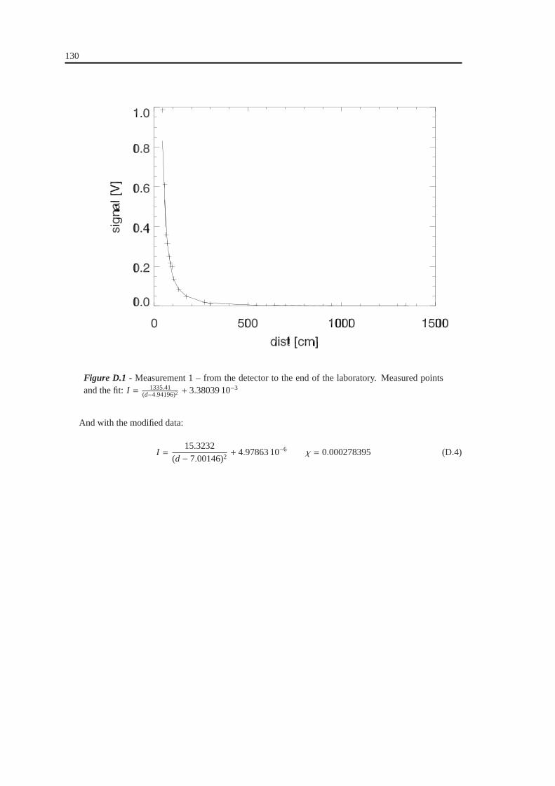
130
Figure D.1 - Measurement 1 – from the detector to the end of the laboratory. Measured pointsand the fit:I = 1335.41
(d−4.94196)2 + 3.38039 10−3
And with the modified data:
I =15.3232
(d − 7.00146)2+ 4.97863 10−6 χ = 0.000278395 (D.4)

APPENDIX D. DISTANCE-SQUARED LAW 131
Figure D.2 - As the previous but in log-log.

132
Figure D.3 - Measurement 2 - from the end of the room towards the detector.Measured pointsand the fit:I = 15.3198
(d−7.00152)2 + 4.60816 10−6
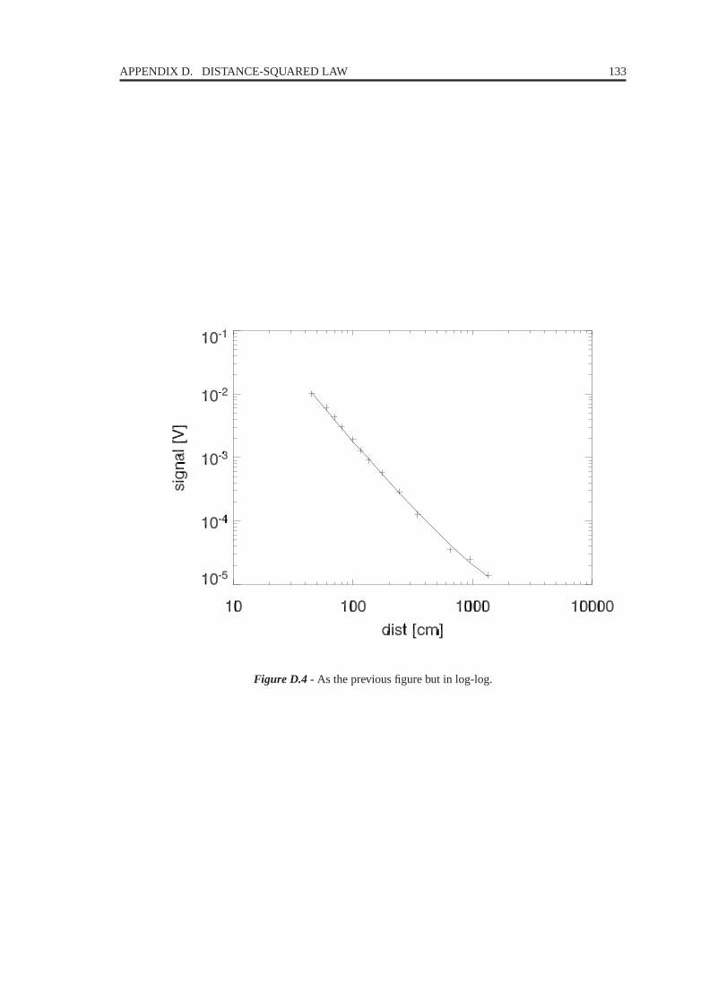
APPENDIX D. DISTANCE-SQUARED LAW 133
Figure D.4 - As the previous figure but in log-log.

134

Appendix EPublications
We reported on our work in three papers:
• Gabor et al.Astronomy& Astrophysics,483:365–369, May 2008.
• Gabor et al.SPIE,vol. 7013, p. 70131R.1 (This paper is an update of the first one, reporting newresults and otherwise only correcting several errors.)
• Gabor et al.SPIE,vol. 7013, p. 70134O.2
The first two papers, dealing with the OPD stabilisation, correspond to Chapter 4, which can be regardedas a corrected and updated version of the papers. Chapter 5 contains the material published in the thirdpaper.
1Published inOptical and Infrared Interferometry.Edited by Scholler, Markus; Danchi, William C.; Delplancke, Francoise.Proceedings of the SPIE, Volume 7013, pp. 70131R-70131R-9 (2008).
2Published inOptical and Infrared Interferometry.Edited by Scholler, Markus; Danchi, William C.; Delplancke, Francoise.Proceedings of the SPIE, Volume 7013, pp. 70134O-70134O-11 (2008).

136
A&A 483, 365–369 (2008)DOI: 10.1051/0004-6361:20077830c© ESO 2008
Astronomy&
Astrophysics
Stabilising a nulling interferometer using
optical path difference dithering
P. Gabor1, B. Chazelas1, F. Brachet2, M. Ollivier1, M. Decaudin1, S. Jacquinod1 , A. Labèque1, and A. Léger1
1 Institut d’Astrophysique Spatiale, 91405 Orsay Cedex, Francee-mail: [email protected]
2 Centre National d’Études Spatiales, 3140 Toulouse Cedex 9, France
Received 9 May 2007 / Accepted 20 February 2008
Abstract
Context. Nulling interferometry has been suggested as the underlying principle for the Darwin and TPF-I exoplanet research missions.Aims. There are constraints both on the mean value of the nulling ratio, and on its stability. Instrument instability noise is mostdetrimental to the stability of the nulling performance.Methods. We applied a modified version of the classical dithering technique to the optical path difference in the scientific beam.Results. Using only this method, we repeatedly stabilised the dark fringe for several hours. This method alone sufficed to remove the1/ f component of the noise in our setup for periods of 10 min, typically. These results indicate that performance stability may bemaintained throughout the long-duration data acquisitions typical of exoplanet spectroscopy.Conclusions. We suggest that further study of possible stabilisation strategies should be an integral part of Darwin/TPF-I researchand development.
Key words. technique: interferometric – instrumentation: spectrographs – space vehicles: instruments – methods: laboratory
1. Nulling interferometry and exoplanet research
The method proposed for exoplanet research for the Darwin(Karlsson & Kaltenegger 2003, European Space Agency-SCI 12,2000) and TPF-I (Coulter 2003, JPL Publ. 05-5, 2005) missionsis based on nulling interferometry Bracewell (1978) designedto enable IR spectroscopic measurements of exoplanetary atmo-spheres as well as imagery of extrasolar planetary systems. Thechallenge is a daunting one with manifold sources of noise Lay(2004): every photon coming from the exoplanet has to be ac-quired and separated from the noise by all means available. Thisimplies that strategies have to be designed to improve the signal-to-noise ratio (S/N) during the data acquisition stage, while de-veloping efficient algorithms for work with the acquired data.This article comments on the former approach.
Experimental studies of nulling interferometer breadboards(Serabyn 2003; Schmidtlin et al. 2005; Ollivier et al. 2001;Vink et al. 2003; Alcatel 2004; Brachet 2005, etc.) show thateven in simple setups, the interference pattern is unstable, drift-ing with time. Even interferometers breadboarded on an opticalbench in the relatively well-controlled laboratory environment(a priori simpler than the actual Darwin/TPF-I, with its multipletelescopes rotating in space) display drifts.
Chazelas et al. (2006) suggest “that special attention be givento servo systems... for monitoring key quantities such as theoptical path difference (OPD) because these systems [have to]be free of long-term drifts” to obtain the required performancethroughout long integration times, e.g. 10 days. Their papergives a quantitative summary of these effects, using data fromOllivier (1999); Alcatel (2004); Vink et al. (2003), and suggeststhat servo mechanisms, using the signal itself, be employed tocontrol drifts.
Chazelas et al. (2006) find that the “quality of the null” at agiven wavelength and at a given moment in time can be evalu-ated in terms of the contrast in intensity between two adjacentdark and bright fringes. It can be expressed as the “nulling ra-tio” (also referred to as “stellar leakage” because it representsthe stellar flux that the interferometer tries to cancel) due to thenulling instrument
nl(λ, t) =Imin
Imax
where Imin and Imax stand for the intensity of the onaxis darkfringe and of the offaxis bright fringe, respectively. Chazelaset al. (2006) show that two types of requirements must be met:one requirement is imposed upon the mean value of the nullingratio nl(λ, t), and the other upon its stability.
Taking into account the wavelength dependence of thestar/planet contrast, they estimate the required mean null as:
〈nl〉 (λ) = 1.0 × 10⁻⁵
(
λ
7 µm
)3.37
.
If such performance in terms of the mean value is achieved, itsrequired long-term stability (at 7 µm) can be expressed as:
σ〈nl〉(7 µm, 10 days) ≤ 3 × 10⁻⁹.
In order to obtain such a high relative stability, an instrumentwith only white noise is desirable, so that instability is reducedwith integration time τ as τ−1/2.
Courtesy of our colleagues (Ollivier 1999; Alcatel 2004;Vink et al. 2003; Brachet 2005), we were able to analyse theirnulling-experiment data. Unfortunately, in all cases, the powerspectral density (PSD) of the null output displays a strong peak
Article published by EDP Sciences

APPENDIX E. PUBLICATIONS 137
Stabilising a nulling interfer ometerusingoptical path differencedithering: an update
Pavel Gabora, BrunoChazelasb, PeterA. Schullera, FrankBrachetc, MarcOlliviera, MichelDecaudina, Alain Labèquea, PhilippeDureta, SophieJacquinoda, Alain Légera
aInstitut d’AstrophysiqueSpatiale,UniversitédeParis-Sud11,Orsay, France;bObservatoiredeGenève,Genève,Switzerland;
cCentreNationald’EtudesSpatiales,Toulouse,France
ABSTRACT
Nulling interferometryhasbeensuggestedasthe underlyingprinciple for an instrumentwhich could provide direct de-tectionandspectroscopy of Earth-like exo-planets,includingsearchesfor potentialbio-signatures.This paperdocumentsthe potentialof optical pathdifference(OPD) stabilisationwith ditheringmethodsfor improving the meannulling ratioandits stability. Thebasicditheringalgorithm,its refinedversionsandparametertuning,arereviewed. This papertakesup the recentlypresentedresults1 andprovidesan updateon OPD-stabilisationat significantlyhigher levels of nullingperformance.
Keywords: Nulling interferometry- Darwin/TPF-I - opticalpathstabilisation- opticalpathdifferencedithering
1. NULLING INTERFEROMETRY AND EXOPLANET RESEARCH
The methodproposedfor exoplanetresearchfor the Darwin2 andTPF-I3 missionsis basedon nulling interferometry4
designedto enableIR spectroscopicmeasurementsof exoplanetaryatmospheresaswell asimageryof extrasolarplanetarysystems.Thechallengeis a dauntingonewith manifoldsourcesof noise:5 every photoncomingfrom theexoplanethasto be acquiredandseparatedfrom the noiseby all meansavailable. This implies that strategieshave to be designedtoimprove the signal-to-noiseratio (S/N) during the dataacquisitionstage,while developingefficient algorithmsfor workwith theacquireddata.This articlecommentson theformerapproach.
Experimentalstudiesof nulling interferometerbreadboards6–11show thatevenin simplesetups,theinterferencepatternis unstable,drifting with time. Even interferometersbreadboardedon an optical benchin the relatively well-controlledlaboratoryenvironment(a priori simpler than the actualDarwin/TPF-I, with its multiple telescopesrotating in space)displaydrifts.
Chazelaset al.12 suggest“that specialattentionbe given to servo systems...for monitoringkey quantitiessuchasthe optical path difference(OPD) becausethesesystems[have to] be free of long-termdrifts” to obtain the requiredperformancethroughoutlong integrationtimes,e.g. 10 days. Their papergives a quantitative summaryof theseeffects,usingdatafrom,9,10,13 andsuggeststhatservo mechanisms,usingthesignalitself, beemployedto controldrifts.
Chazelasetal.12 find thatthe“quality of thenull” atagivenwavelengthandatagivenmomentin timecanbeevaluatedin termsof thecontrastin intensitybetweentwo adjacentdarkandbright fringes.It canbeexpressedasthe“nulling ratio”(alsoreferredto as“stellar leakage”becauseit representsthestellarflux that theinterferometertriesto cancel)dueto thenulling instrument
nl(λ, t) =Imin
Imax
Correspondingauthor:[email protected];Institut d’AstrophysiqueSpatiale,bât. 121,CampusScientifique,91405Orsay, France;phone+33 1 69 85 87 32.

138
Tests of achromatic phase shifters performed on the SYNAPSE
test bench: a progress report
Pavel Gabora, Peter A. Schullera, Bruno Chazelasb, Michel Decaudina, Alain Labequea,
Philippe Dureta, Yves Rabbiac, Ralf Launhardtd, Jean Gayc, Zoran Sodnike, Marc Barillotf,
Frank Brachetg, Thomas Laurenth, Sophie Jacquinoda, Denis Vandormaeli, Jerome Loicqi,
Dimitri Mawetj, Marc Olliviera, Alain Legera
aInstitut d’Astrophysique Spatiale, Univ. Paris-Sud 11, Orsay, France;bObservatoire de Geneve, Geneve, Switzerland;cObservatoire de la Cote d’Azur, Nice, France;
dMax-Planck-Institut fur Astronomie, Heidelberg, Germany;eEuropean Space Agency, Nordwijk, Netherlands;fThales Alenia Space, Cannes La Bocca, France;
gCentre National d’Etudes Spatiales, Toulouse, France;hUniv. Liege, Liege, Belgium;
iCentre Spatial de Liege, Liege, Belgium;jUniv. Liege, Institut d’Astrophysique et de Geophysique, Liege, Belgium
ABSTRACT
The achromatic phase shifter (APS) is a component of the Bracewell nulling interferometer studied in preparationfor future space missions (viz. Darwin/TPF-I) focusing on spectroscopic study of Earth-like exo-planets. Severalpossible designs of such an optical subsystem exist. Four approaches were selected for further study. ThalesAlenia Space developed a dielectric prism APS. A focus crossing APS prototype was developed by the OCA,Nice, France. A field reversal APS prototype was prepared by the MPIA in Heidelberg, Germany. Centre Spatialde Liege develops a concept based on Fresnel’s rhombs. This paper presents a progress report on the currentwork aiming at evaluating these prototypes on the Synapse test bench at the Institut d’Astrophysique Spatialein Orsay, France.
Keywords: Nulling interferometry, exoplanets, infrared spectroscopy, Darwin/TPF-I, achromatic phase shifters
1. NULLING INTERFEROMETRY AND ACHROMATIC PHASE SHIFTERS
Nulling interferometry, based on the concept suggested by Bracewell1 in 1978, is one of the methods of futureexoplanet research. It has been studied for the mission Darwin
2 proposed to ESA as well as for the missionTPF-I (Terrestrial Planet Finder - Interferometry)3 proposed to NASA.
The basic performance parameter of a nulling interferometer is the “nulling ratio” (sometimes also referredto as “stellar leakage” although this term refers more properly to stray starlight due to the fact a star is not apoint source) nl(λ, t) = Imin/Imax where Imin and Imax stand for the intensity of the on-axis dark fringe and ofthe off-axis bright fringe, respectively.
The goal of Darwin/TPF-I is to perform infra-red (6 − 18µm) imagery of extrasolar planetary systems andspectroscopic observations of exoplanetary atmospheres in view of evaluating the presence of biomarkers. In orderto reach this goal, the required nulling performance has been estimated4 as 〈nl〉 (λ) = 1.0 10−5 (λ/7µm)
3.37,
with a level of long-term stability expressed as σ〈nl〉(7µm, 10 days) ≤ 3 10−9.
Corresponding author: [email protected]; Institut d’Astrophysique Spatiale, bat. 121, Campus Scientifique, 91405
Orsay, France; phone +33 1 69 85 87 32.

List of Figures
1.1 Sun-Earth contrast. . . . . . . . . . . . . . . . . . . . . . . . . . . . . . . . . . . . . . 8
1.2 TPF Coronograph. . . . . . . . . . . . . . . . . . . . . . . . . . . . . . . . . . . . . . . 8
1.3 New Worlds Observer. . . . . . . . . . . . . . . . . . . . . . . . . . . . . . . . . . . . . 9
1.4 Darwin/TPF-I space observatory.. . . . . . . . . . . . . . . . . . . . . . . . . . . . . . . 10
1.5 Provenance of the photons detected byDarwin/TPF-I . . . . . . . . . . . . . . . . . . . . 11
1.6 Darwin/TPF-I rotation modulation. . . . . . . . . . . . . . . . . . . . . . . . . . . . . . 12
1.7 Simulation of an interferometer’s transmission. . . . . . . . . . . . . . . . . . . . . . . . 12
2.1 Bracewell’s nulling interferometer. . . . . . . . . . . . . . . . . . . . . . . . . . . . . . 16
2.2 Four APS concepts. . . . . . . . . . . . . . . . . . . . . . . . . . . . . . . . . . . . . . 19
2.3 Dispersive Prisms APS: principle. . . . . . . . . . . . . . . . . . . . . . . . . . . . . . . 21
2.4 Map of the (OPD,e) space . . . . . . . . . . . . . . . . . . . . . . . . . . . . . . . . . . 21
2.5 Three OPD scans for different values ofe. . . . . . . . . . . . . . . . . . . . . . . . . . . 22
2.6 The “Lawson” plot . . . . . . . . . . . . . . . . . . . . . . . . . . . . . . . . . . . . . . 24
3.1 Global view of Marc Ollivier’s testbed.. . . . . . . . . . . . . . . . . . . . . . . . . . . . 29
3.2 Global view of S, September 2003.. . . . . . . . . . . . . . . . . . . . . . . . . . 30
3.3 The original, cryogenic, version of N . . . . . . . . . . . . . . . . . . . . . . . . 31
3.4 General view of N (during alignment).. . . . . . . . . . . . . . . . . . . . . . . 31
3.5 A view of the P testbed.. . . . . . . . . . . . . . . . . . . . . . . . . . . . . . . . . 32
3.6 S: decoupling of the interferometer from the source and detector . . . . . . . . . . 34
3.7 S: plexiglass enclosure with top-side heating. . . . . . . . . . . . . . . . . . . . . 34
3.8 N on its optical table, with protective casing.. . . . . . . . . . . . . . . . . . . . 35
3.9 Uni-axial and multi-axial beam combination. . . . . . . . . . . . . . . . . . . . . . . . . 37
3.10 Serabyn-Colavita modified Mach-Zehnder beam splitter. . . . . . . . . . . . . . . . . . . 39
3.11 Serabyn-Colavita modified Mach-Zehnder beam combiner. . . . . . . . . . . . . . . . . 39
3.12 Flux mismatch estimation. . . . . . . . . . . . . . . . . . . . . . . . . . . . . . . . . . . 40
3.13 Ceramic black body (a cross-section).. . . . . . . . . . . . . . . . . . . . . . . . . . . . 45

140 LIST OF FIGURES
3.14 Structure of the 1.15µm laser beam . . . . . . . . . . . . . . . . . . . . . . . . . . . . . 46
3.15 Spectrum of a supercontinuum laser source.. . . . . . . . . . . . . . . . . . . . . . . . . 47
3.16 Transmission of the K-band single-mode fibre. . . . . . . . . . . . . . . . . . . . . . . . 49
3.17 Transmission of the K-band single-mode fibre. . . . . . . . . . . . . . . . . . . . . . . . 49
3.18 K filter transmission. . . . . . . . . . . . . . . . . . . . . . . . . . . . . . . . . . . . . . 50
3.19 K’ filter transmission. . . . . . . . . . . . . . . . . . . . . . . . . . . . . . . . . . . . . 51
3.20 L filter transmission. . . . . . . . . . . . . . . . . . . . . . . . . . . . . . . . . . . . . . 51
3.21 Narrow K filter transmission. . . . . . . . . . . . . . . . . . . . . . . . . . . . . . . . . 52
3.22 Transmission curves of P03 polarisers. (Courtesy InfraSpecs). . . . . . . . . . . . . . . . 52
3.23 Focus Crossing APS prototype. . . . . . . . . . . . . . . . . . . . . . . . . . . . . . . . 53
3.24 Field Reversal APS prototype. . . . . . . . . . . . . . . . . . . . . . . . . . . . . . . . . 54
3.25 Dispersive Prisms APS prototype. . . . . . . . . . . . . . . . . . . . . . . . . . . . . . . 54
3.26 Stanford Research Systems SR830 Lock-In Amplifier.. . . . . . . . . . . . . . . . . . . 55
3.27 The first SW system. “Real time.”. . . . . . . . . . . . . . . . . . . . . . . . . . . . . . 57
3.28 The first SW system. Routines running on the PC. . . . . . . . . . . . . . . . . . . . . . 57
3.29 The first SW system. Routines running on the PXI. . . . . . . . . . . . . . . . . . . . . . 58
3.30 The second SW system.. . . . . . . . . . . . . . . . . . . . . . . . . . . . . . . . . . . . 59
3.31 The third SW system. . . . . . . . . . . . . . . . . . . . . . . . . . . . . . . . . . . . . 61
3.32 Images of S overlaid with science and metrology beams. . . . . . . . . . . . . . . 62
3.33 Metrology beam splitter.. . . . . . . . . . . . . . . . . . . . . . . . . . . . . . . . . . . 63
3.34 S layout . . . . . . . . . . . . . . . . . . . . . . . . . . . . . . . . . . . . . . . . 64
3.35 N: outline of the optical layout. . . . . . . . . . . . . . . . . . . . . . . . . . . 65
3.36 N. Line-point-plane mechanics. . . . . . . . . . . . . . . . . . . . . . . . . . . 66
4.1 S K-band results. . . . . . . . . . . . . . . . . . . . . . . . . . . . . . . . . . . . 69
4.2 Smeasurement with the external-metrology stabilisation. . . . . . . . . . . . . . . 69
4.3 OPD dithering cycle.. . . . . . . . . . . . . . . . . . . . . . . . . . . . . . . . . . . . . 71
4.4 Oscilloscope measurements.. . . . . . . . . . . . . . . . . . . . . . . . . . . . . . . . . 73
4.5 OPD-stabilised data acquisition. . . . . . . . . . . . . . . . . . . . . . . . . . . . . . . . 73
4.6 OPD-stabilised null’s PSD and running averageσ. . . . . . . . . . . . . . . . . . . . . . 74
4.7 OPD stabilisation with a HeNe laser at 3.39µm . . . . . . . . . . . . . . . . . . . . . . . 76
4.8 Comparison with other experiments.. . . . . . . . . . . . . . . . . . . . . . . . . . . . . 78
5.1 Fringe dispersion technique. . . . . . . . . . . . . . . . . . . . . . . . . . . . . . . . . . 84
5.2 S K-band results. . . . . . . . . . . . . . . . . . . . . . . . . . . . . . . . . . . . 87
5.3 Stabilised HeNe. . . . . . . . . . . . . . . . . . . . . . . . . . . . . . . . . . . . . . . . 88
6.1 S beam profiles (infrared pinhole scans).. . . . . . . . . . . . . . . . . . . . . . . 95
6.2 Lateral dispersion. . . . . . . . . . . . . . . . . . . . . . . . . . . . . . . . . . . . . . . 96
6.3 Air column equality among the pairs of CaF2 Prisms . . . . . . . . . . . . . . . . . . . . 97

LIST OF FIGURES 141
6.4 Injection shear. . . . . . . . . . . . . . . . . . . . . . . . . . . . . . . . . . . . . . . . . 98
6.5 Injection tip/tilt . . . . . . . . . . . . . . . . . . . . . . . . . . . . . . . . . . . . . . . . 99
6.6 Nulling measurement at different CaF2 working points . . . . . . . . . . . . . . . . . . . 100
6.7 Spectral mismatch verification. . . . . . . . . . . . . . . . . . . . . . . . . . . . . . . . 101
B.1 Stellar leakage. . . . . . . . . . . . . . . . . . . . . . . . . . . . . . . . . . . . . . . . . 122
B.2 Mathematical model of the 1/ f noise. . . . . . . . . . . . . . . . . . . . . . . . . . . . . 124
B.3 RequiredDarwin/TPF-I stability . . . . . . . . . . . . . . . . . . . . . . . . . . . . . . . 124
C.1 Parabola. . . . . . . . . . . . . . . . . . . . . . . . . . . . . . . . . . . . . . . . . . . . 126
C.2 Encircled power. Linear plot. . . . . . . . . . . . . . . . . . . . . . . . . . . . . . . . . 127
C.3 Encircled power. Semilogarithmic plot. . . . . . . . . . . . . . . . . . . . . . . . . . . . 127
C.4 Coupling efficiency . . . . . . . . . . . . . . . . . . . . . . . . . . . . . . . . . . . . . . 128
D.1 Measurement 1 (linear scale). . . . . . . . . . . . . . . . . . . . . . . . . . . . . . . . . 130
D.2 Measurement 1 (logarithmic scale). . . . . . . . . . . . . . . . . . . . . . . . . . . . . . 131
D.3 Measurement 2 (linear scale). . . . . . . . . . . . . . . . . . . . . . . . . . . . . . . . . 132
D.4 Measurement 2 (logarithmic scale). . . . . . . . . . . . . . . . . . . . . . . . . . . . . . 133

142 LIST OF FIGURES

List of Tables
2.1 Main nulling-interferometry results of various teams.. . . . . . . . . . . . . . . . . . . . 25
3.1 The 2nd and 3rd SW system. Commands implemented on the server . . . . . . . . . . . . 59
4.1 Stabilisation results with a ceramic black body source. . . . . . . . . . . . . . . . . . . . 75
4.2 Stabilisation results with a 3.39µm laser. . . . . . . . . . . . . . . . . . . . . . . . . . . 76
5.1 Photometry of S . . . . . . . . . . . . . . . . . . . . . . . . . . . . . . . . . . . . 83
5.2 S II results . . . . . . . . . . . . . . . . . . . . . . . . . . . . . . . . . . . . . . . 89
5.3 S II results with the Focus Crossing APS. . . . . . . . . . . . . . . . . . . . . . . 90
5.4 S II results with the narrow passband filter. . . . . . . . . . . . . . . . . . . . . . 90
5.5 S progress overview. . . . . . . . . . . . . . . . . . . . . . . . . . . . . . . . . . 92
6.1 Error budget. . . . . . . . . . . . . . . . . . . . . . . . . . . . . . . . . . . . . . . . . . 103

144 LIST OF TABLES

Bibliography
Review and discussion of APS requirements, ESA AO/1-3946/02/NL/JA. Technical report, 2002.
Alcatel. private communication from Alcatel Space Industries (now Thales Alenia Space), 2004.
J. R. P. Angel and N. J. Woolf. An Imaging Nulling Interferometer to Study Extrasolar Planets.Astrophys-ical Journal, 475:373–+, January 1997. doi: 10.1086/303529.
P. Baudoz, Y. Rabbia, and J. Gay. Achromatic interfero coronagraphy I. Theoretical capabilities for ground-based observations.Astronomy and Astrophysics, 141:319–329, January 2000a.
P. Baudoz, Y. Rabbia, J. Gay, R. Burg, L. Petro, P. Bely, B. Fleury, P.-Y. Madec, and F. Charbonnier.Achromatic interfero coronagraphy. II. Effective performance on the sky.Astronomy and Astrophysics,145:341–350, August 2000b.
C.A. Beichman, N.J. Woolf, and C.A. Lindensmith.The Terrestrial Planet Finder (TPF), JPL 99-3. NASA,1999. URLhttp://planetquest.jpl.nasa.gov/TPF/tpf_book/index.cfm.
Matthieu Boffety and David Drugeon.Etude du dephasage introduit par un dephaseur achromatique. Mas-ter’s thesis,Ecole superieure d’optique, 2006.
H. Bokhove, J. P. Kappelhof, H. J. P. Vink, L. L. A. Vosteen, and Z. Sodnik. Broadband nulling using aprism phase shifter. InESA SP-539: Earths: DARWIN/TPF and the Search for Extrasolar TerrestrialPlanets, pages 367–369, October 2003.
R. W. Boyd. Intuitive explanation of the phase anomaly of focused light beams.Journal of the OpticalSociety of America (1917-1983), 70:877–+, 1980.
R. N. Bracewell. Detecting nonsolar planets by spinning infrared interferometer.Nature, 274:780–+,August 1978.
Frank Brachet. Etude et developpement d’un dephaseur achromatique pourl’interferometrie en frangenoire. PhD thesis, Paris XI, 2005.
C. Buisset, X. Rejeaunier, Y. Rabbia, and M. Barillot. Stable deep nulling in polychromatic unpolarizedlight with multiaxial beam combination.Applied Optics, 46:7817–7822, November 2007. doi: 10.1364/AO.46.007817.
Christophe Buisset.Caracterisation et optimisation d’un interferometre `a frange sombre et a bande large.PhD thesis, Nice, 2007.
B. Chazelas, F. Brachet, P. Borde, B. Mennesson, M. Ollivier, O. Absil, A. Labeque, C. Valette, andA. Leger. Instrumental stability requirements for exoplanet detection with a nulling interferometer :variability noise is a central issue.Applied Optics, 45(5):984–992, 2006.
146 BIBLIOGRAPHY
Bruno Chazelas.Contribution a l’etude de l’interferometrie annulante pour la detection d’exo-planetes.PhD thesis, Paris XI, 2007.
V. Coude Du Foresto, G. Perrin, C. Ruilier, B. P. Mennesson, W. A. Traub, and M. G. Lacasse. FLUORfibered instrument at the IOTA interferometer. In R. D. Reasenberg, editor,Society of Photo-OpticalInstrumentation Engineers (SPIE) Conference Series, volume 3350 ofPresented at the Society of Photo-Optical Instrumentation Engineers (SPIE) Conference, pages 856–863, July 1998.
Michael J. Crowe.The Extraterrestrial Life Debate, 1750–1900. Dover Publications, 1999.
Rene Descartes.Principia philosophiae. 1644.
Steven J. Dick.Plurality of Worlds: The Extraterrestrial Life Debate fromDemocritus to Kant. CambridgeUniversity Press, 1984.
Steven J. Dick.Life on Other Worlds: The 20th Century Extraterrestrial Life Debate. Cambridge UniversityPress, 1996.
F. D. Drake. Project Ozma.Physics Today, 14:40–+, 1961.
Frank Drake and Dava Sobel.Is Anyone Out There? The Scientific Search for Extraterrestrial Intelligence.Delacorte Pr., New York, 1992.
G. Faure and T. Mensing.Introduction to planetary science. The geological perspective. Springer, 2007.
R. Flatscher, Z. Sodnik, K. Ergenzinger, U. Johann, and R. Vink. DARWIN nulling interferometer bread-board I: System engineering and measurements. InESA SP-539: Earths: DARWIN/TPF and the Searchfor Extrasolar Terrestrial Planets, pages 283–291, October 2003.
Bernard le Bovier de Fontenelle.Entretiens sur la pluralite des mondes. 1686.
Fragment. From Anaxagoras quoted by Simplicius of Cilicia.B4a.
Fragment. From Simplicius of Cilicia quoted by Theophrastus,Φυσικων ∆oξαι. Phys. opin. 4, 7.
P. Gabor, B. Chazelas, F. Brachet, M. Ollivier, M. Decaudin,S. Jacquinod, A. Labeque, and A. Leger.Stabilising a nulling interferometer using optical path difference dithering.Astronomy& Astrophysics,483:365–369, May 2008a. doi: 10.1051/0004-6361:20077830.
P. Gabor, B. Chazelas, P. A. Schuller, F. Brachet, M. Ollivier, M. Decaudin, A. Labeque, P. Duret,S. Jacquinod, and A. Leger. Stabilising a nulling interferometer using optical path difference dithering:an update. InSociety of Photo-Optical Instrumentation Engineers (SPIE) Conference Series, volume7013 ofSociety of Photo-Optical Instrumentation Engineers (SPIE) Conference Series, July 2008b. doi:10.1117/12.789222.
P. Gabor, P. A. Schuller, B. Chazelas, M. Decaudin, A. Labeque, P. Duret, Y. Rabbia, R. Launhardt, J. Gay,Z. Sodnik, M. Barillot, F. Brachet, T. Laurent, S. Jacquinod, D. Vandormael, J. Loicq, D. Mawet, M. Ol-livier, and A. Leger. Tests of achromatic phase shifters performed on the SYNAPSE test bench: aprogress report. InSociety of Photo-Optical Instrumentation Engineers (SPIE) Conference Series, vol-ume 7013 ofSociety of Photo-Optical Instrumentation Engineers (SPIE) Conference Series, July 2008c.doi: 10.1117/12.789269.
Pavel Gabor. Achromatic phase shifter performance stabilisation through optical path difference modula-tion. Master’s thesis, Master Recherche (M2) Astronomie etAstrophysique, Universite Paris VII, 2006.
R. O. Gappinger, R. T. Diaz, A. Ksendzov, P. R. Lawson, O. P. Lay, K. M. Liewer, F. M. Loya, S. R.Martin, E. Serabyn, and J. K. Wallace. Experimental evaluation of achromatic phase shifters for mid-infrared starlight suppression.Applied Optics, 48:868–+, February 2009. doi: 10.1364/AO.48.000868.
Stephen Gaukroger.The emergence of a scientific culture. Science and the shaping of modernity, 1210–1685. Oxford University Press, 2006.
BIBLIOGRAPHY 147
Jean Gay and Yves Rabbia.C.R. Acad.Sci. Paris, IIb, 322:265, 1996.
A. Gelb and W. E. Vander Velde.Multiple-Input Describing Functions and Nonlinear SystemDesign.McGraw-Hill, New York, 1968.
Anthony Gottlieb.Particle Man.A review of Rowland’sGiordano Bruno. Philosopher/Heretic. New YorkTimes, 19 Dec 2008.
G. Gouy.C.R. Acad.Sci. Paris, 110:1251, 1890.
Pierre Haguenauer and Eugene Serabyn. Deep nulling of laserlight with a single-mode-fiber beam combiner. Applied Optics, 45(12):2749–2754, 2006. URLhttp://ao.osa.org/abstract.cfm?URI=ao-45-12-2749.
K. Houairi, F. Cassaing, J. M. Le Duigou, B. Sorrente, S. Jacquinod, and J. P. Amans. PERSEE, thedynamic nulling demonstrator: recent progress on the cophasing system. InSociety of Photo-OpticalInstrumentation Engineers (SPIE) Conference Series, volume 7013 ofPresented at the Society of Photo-Optical Instrumentation Engineers (SPIE) Conference, July 2008. doi: 10.1117/12.789113.
Kamel Houairi.Cophasage de telescopes multi-pupilles sur point source: application a linterferomtre enfrange noire Persee. PhD thesis, Observatoire de Paris, oct. 2009.
E. M. Jones. Where is everybody? An account of Fermi’s question. Physics Today, pages 11–13, Aug 1985.
Charles H. Kahn.Anaximander and the origins of Greek cosmology, page 52. Columbia Unversity Press,1960.
L. Kaltenegger, W. A. Traub, and K. W. Jucks. Spectral Evolution of an Earth-like Planet.AstrophysicalJournal, 658:598–616, March 2007. doi: 10.1086/510996.
A. Ksendzov, O. Lay, S. Martin, J. S. Sanghera, L. E. Busse, W.H. Kim, P. C. Pureza, V. Q. Nguyen, andI. D. Aggarwal. Characterization of mid-infrared single mode fibers as modal filters.Applied Optics, 46:7957–7962, November 2007.
L. Labadie, E. Le Coarer, R. Maurand, P. Labeye, P. Kern, B. Arezki, and J.-E. Broquin. Mid-infrared laserlight nulling experiment using single-mode conductive waveguides.Astronomy and Astrophysics, 471:355–360, August 2007. doi: 10.1051/0004-6361:20067005.
Ralf Launhardt. Breadboarding an achromatic phase shifterfor midinfrared nulling interferometry. volume7013 ofTo be presented at the Society of Photo-Optical Instrumentation Engineers (SPIE) Conference,pages paper 7013–175, June 2008.
Thomas Laurent. Participatona l’experience d’interferometrie annulante S: validation des technolo-gies de la mission spatiale Darwin. Master’s thesis, Universite de Liege, 2008.
P. R. Lawson, O. P. Lay, and C. A. Beichman.Terrestrial Planet Finder Interferometer Science WorkingGroup Report. NASA, 2007.
P. R. Lawson, O. P. Lay, S. R. Martin, R. D. Peters, R. O. Gappinger, A. Ksendzov, and D. P. Scharf. Tech-nology challenges for exoplanet detection with mid-IR interferometry. In7th International Conferenceon Space Optics, 14-17 October, Toulouse, France, October 2008.
Peter R. Lawson. Nulling interferometry and the detection of Earth-like planets. state of the art., 2009. URLhttp://planetquest.jpl.nasa.gov/TPF-I/stateOfTheArt.cfm.
P.R. Lawson and J.A. Dooley.Technology Plan for the Terrestrial Planet Finder Interferometer, JPL 05-5.NASA, 2005. URLhttp://planetquest.jpl.nasa.gov/Navigator/library/tpfI414.pdf.
O. P. Lay. Removing instability noise in nulling interferometers. InSociety of Photo-Optical Instrumen-tation Engineers (SPIE) Conference Series, volume 6268 ofSociety of Photo-Optical InstrumentationEngineers (SPIE) Conference Series, July 2006. doi: 10.1117/12.670603.
148 BIBLIOGRAPHY
O. P. Lay. Systematic errors in nulling interferometers.Applied Optics, 43:6100–6123, 2004.
J. Lazio, T. Bastian, G. Bryden, W. M. Farrell, J.-M. Griessmeier, G. Hallinan, J. Kasper, T. Kuiper,A. Lecacheux, W. Majid, R. Osten, E. Shklonik, I. Stevens, D.Winterhalter, and P. Zarka. Magneto-spheric Emissions from Extrasolar Planets.Astronomy, 2010:177–+, 2009.
A. Leger, J-M. Mariotti, J-L. Puget, D. Rouan, and J. Schneider.DARWIN: Mission concept for the ESAHorizon 2000+ program.ESA, 1993.
A. Leger, M. Ollivier, K. Altwegg, and N. J. Woolf.Astronomy and Astrophysics, 341:304, 1999.
S. Martin, P. Szwaykowski, and F. Loya. Testing exo-planet signal extraction using the Terrestrial PlanetFinder planet detection testbed. In D. R. Coulter, editor,Society of Photo-Optical Instrumentation En-gineers (SPIE) Conference Series, volume 5905 ofSociety of Photo-Optical Instrumentation Engineers(SPIE) Conference Series, pages 70–79, August 2005. doi: 10.1117/12.615559.
S. R. Martin, R. O. Gappinger, F. M. Loya, B. P. Mennesson, S. L. Crawford, and E. Serabyn. Mid-infrarednuller for Terrestrial Planet Finder: design, progress, and results. InTechniques and Instrumentationfor Detection of Exoplanets. Edited by Coulter, Daniel R. Proceedings of the SPIE, Volume 5170, pp.144-154 (2003)., pages 144–154, November 2003a. doi: 10.1117/12.521312.
S. R. Martin, E. Serabyn, and G. Hardy. Deep nulling of laser light in a rotational shearing interferometer.In Interferometry for Optical Astronomy II. Edited by Wesley A. Traub. Proceedings of the SPIE, Volume4838., pages 656–667, February 2003b.
S. R. Martin, P. Szwaykowski, F. M. Loya, and K. Liewer. Progress in testing exo-planet signal extraction onthe TPF-I planet detection testbed. InSociety of Photo-Optical Instrumentation Engineers (SPIE) Con-ference Series, volume 6268 ofSociety of Photo-Optical Instrumentation Engineers (SPIE) ConferenceSeries, July 2006. doi: 10.1117/12.672646.
J. Lewis McIntyre.Giordano Bruno. 1992.
B. Mennesson, M. Ollivier, and C. Ruilier. Use of single-mode waveguides to correct the optical defects ofa nulling interferometer.Optical Society of America Journal, 19:596–602, March 2002.
B. Mennesson, S. L. Crawford, E. Serabyn, S. Martin, M. Creech-Eakman, and G. Hardy. Laboratoryperformance of the Keck Interferometer nulling beam combiner. InESA SP-539: Earths: DARWIN/TPFand the Search for Extrasolar Terrestrial Planets, pages 525–528, October 2003.
B. Mennesson, A. Leger, and M. Ollivier. Direct detection and characterization of extrasolar planets: TheMariotti space interferometer.Icarus, 178:570–588, November 2005. doi: 10.1016/j.icarus.2005.05.012.
B. Mennesson, P. Haguenauer, E. Serabyn, and K. Liewer. Deepbroad-band infrared nulling using a single-mode fiber beam combiner and baseline rotation. InSociety of Photo-Optical Instrumentation Engineers(SPIE) Conference Series, volume 6268 ofPresented at the Society of Photo-Optical InstrumentationEngineers (SPIE) Conference, July 2006. doi: 10.1117/12.672157.
R. M. Morgan, J. H. Burge, and N. J. Woolf. Final laboratory results of visible nulling with dielectric plates.In Interferometry for Optical Astronomy II. Edited by Wesley A. Traub. Proceedings of the SPIE, Volume4838, pp. 644-655 (2003)., pages 644–655, February 2003.
M. Ollivier. Coronographie interferentielle pour la mission Darwin. PhD thesis, Universite Paris XI,December 1999.
M. Ollivier, J.-M. Mariotti, A. Leger, P. Sekulic, J. Brunaud, and G. Michel. Interferometric coronographyfor the DARWIN space mission - Laboratory demonstration experiment. Astronomy and Astrophysics,370:1128–1136, May 2001.

BIBLIOGRAPHY 149
M. Perryman, O. Hainaut, D. Dravins, A. Leger, A. Quirrenbach, H. Rauer, F. Kerber, R. Fosbury,F. Bouchy, F. Favata, M. Fridlund, R. Gilmozzi, A. Lagrange,T. Mazeh, D. Rouan, S. Udry, and J. Wamb-sganss. Report by the ESA-ESO Working Group on Extra-Solar Planets. ArXiv Astrophysics e-prints,June 2005.
R. D. Peters, O. P. Lay, A. Hirai, and M. Jeganathan. Progressin deep broadband interferometric nullingwith the adaptive nuller. InSociety of Photo-Optical Instrumentation Engineers (SPIE) ConferenceSeries, volume 7013 ofPresented at the Society of Photo-Optical InstrumentationEngineers (SPIE)Conference, July 2008. doi: 10.1117/12.786845.
Robert D. Peters, Oliver P. Lay, and Muthu Jeganathan. Broadband phase and intensity compensationwith a deformable mirror for an interferometric nuller.Appl. Opt., 47(21):3920–3926, 2008. URLhttp://ao.osa.org/abstract.cfm?URI=ao-47-21-3920.
Michael Polanyi.Personal Knowledge. Towards a Post-Critical Philosophy. Harper, 1958.
Y. Rabbia, Y. Gay, and E. Bascou. Achromatic phase shifters for nulling interferometry. InICSO’2000- Conference Internationale d’Optique Spatiale, Toulouse, France, Dec. 5-7, 2000) CNES Eds., pages389–400, 2000.
Y. Rabbia, Y. Gay, E. Bascou, and J. L. Schneider. Summary assessment report on achromatic phase shiftersfor space interferometry. Technical report, ESA ESTEC, Contract 14 398/00/NL/MV, 2001.
Y. Rabbia, J. Gay, B. Chazelas, A. Labeque, and J.-P. Rivet. Nulling interferometry : Lommel’s integralsapplied to a Fresnel’s diffraction effect. In C. Aime and F. Vakili, editors,IAU Colloq. 200: DirectImaging of Exoplanets: Science& Techniques, pages 265–270, 2006. doi: 10.1017/S1743921306009434.
Ingrid D. Rowland.Giordano Bruno. Philosopher/Heretic. Farrar, Strauss & Giroux, 2008.
Carl Sagan.Cosmos. Random House, 1980.
R. Samuele, J. K. Wallace, E. Schmidtlin, M. Shao, B. M. Levine, and S. Fregoso. Experimental progressand results of a visible nulling coronagraph. InProceedings of IEEE Aerospace Conference. Institute ofElectrical and Electronic Engineers, 2007.
N. C. Santos, G. Israelian, M. Mayor, R. Rebolo, and S. Udry. Statistical properties of exoplanets. II.Metallicity, orbital parameters, and space velocities.Astronomy& Astrophysics, 398:363–376, January2003. doi: 10.1051/0004-6361:20021637.
E. Schmidtlin, J. K. Wallace, R. Samuele, B. M. Levine, and M.Shao. Recent Progress of Visible LightNulling Interferometry and First 1 Million Null Result. In CAime and F. Vakili, editors,Direct Imagingof Exoplanets: Science and Techniques, pages 353–360. IAU Colloquium No. 200, 2005.
F. Selsis, D. Despois, and J.-P. Parisot.Astronomy and Astrophysics, 388:985, 2002.
E. Serabyn. Nulling interferometry progress. In Wesley A. Traub, editor,Interferometry for Optical As-tronomy II. Proceedings of the SPIE, volume 4838, pages 594–608, February 2003.
E. Serabyn. Nulling interferometry: symmetry requirements and experimental results. In P. Lena & A. Quir-renbach, editor,Society of Photo-Optical Instrumentation Engineers (SPIE) Conference Series, volume4006 ofSociety of Photo-Optical Instrumentation Engineers (SPIE) Conference Series, pages 328–339,July 2000.
E. Serabyn and M. Colavita. Fully symmetric nulling beam combiners.Applied Optics, 40:1668, 2001.
E. Serabyn and M. M. Colavita. Fully Symmetric Nulling Beam Combiners.Applied Optics, 40:1668–1671,April 2001.
I. S. Shklovskii and C. Sagan.Intelligent life in the universe. Random House, 1966.
DanielSpelda.Astronomie v antice [Astronomy in Antiquity]. Montanex, Ostrava, 2006.

150 BIBLIOGRAPHY
J. Spronck, S. F. Pereira, and J. J. M. Braat. Chromatism compensation in wide-band nulling interferometryfor exoplanet detection.Applied Optics, 45:597–604, February 2006. doi: 10.1364/AO.45.000597.
James Strick. Darwin and the origin of life: A historical perspective.American Associaiton for the Advance-ment of Science, Workshop “Exploring the Origin, Extent, and Future of Life: Philosophical, Ethical, andTheological Perspectives”, Feb 2003.
Leonard Susskind.The Cosmic Landscape: String Theory and the Illusion of Intelligent Design. Back BayBooks, 2006.
A. V. Tavrov, Y. Otani, T. Kurokawa, and M. Takeda. 3D common-path interferometer: achromatic nullingof on-axial light. In D. R. Coulter, editor,Society of Photo-Optical Instrumentation Engineers (SPIE)Conference Series, volume 5905 ofSociety of Photo-Optical Instrumentation Engineers (SPIE) Confer-ence Series, pages 398–404, August 2005. doi: 10.1117/12.620027.
The Stanford encyclopedia of philosophy. The entry on Anaxagoras. 2007.
H. J. P. Vink, N. J. Doelman, R. Flatscher, and Z. Sodnik. DARWIN nulling interferometer breadboardII: design and manufacturing. InESA SP-539: Earths: DARWIN/TPF and the Search for ExtrasolarTerrestrial Planets, pages 641–645, October 2003.
L. L. A. Vosteen, H. J. P. Vink, H. van Brug, and H. Bokhove. Achromatic phase-shifter breadboard exten-sions. In D. R. Coulter, editor,Society of Photo-Optical Instrumentation Engineers (SPIE) ConferenceSeries, volume 5905 ofSociety of Photo-Optical Instrumentation Engineers (SPIE) Conference Series,pages 91–101, August 2005. doi: 10.1117/12.614337.
J. K. Wallace, M. Shao, B. F. Lane, B. M. Levine, F. Loya, A. Azizi, B. Holmes, F. Aguayo, J. Negron,G. Sanchez, and R. O. Gappinger. Experimental results from the optical planet detector interferometer.In D. R. Coulter, editor,Society of Photo-Optical Instrumentation Engineers (SPIE) Conference Series,volume 5170 ofSociety of Photo-Optical Instrumentation Engineers (SPIE) Conference Series, pages209–216, November 2003. doi: 10.1117/12.506356.
J. K. Wallace, V. Babtiwale, R. Bartos, K. Brown, R. Gappinger, F. Loya, D. MacDonald, S. Martin,J. Negron, T. Truong, and G. Vasisht. Mid-IR interferometric nulling for TPF. InNew Frontiers inStellar Interferometry, Proceedings of SPIE Volume 5491. Edited by Wesley A. Traub. Bellingham, WA:The International Society for Optical Engineering, 2004.,p.862, pages 862–+, October 2004.
K. Wallace, G. Hardy, and E. Serabyn. Deep and stable interferometric nulling of broadband light withimplications for observing planets around nearby stars.Nature, 406:700–702, August 2000.
Stephen Webb.If the Universe is teeming with aliens... Where is everybody? Fifty solutions to the FermiParadox and the problem of extraterrestrial life. Springer, 2002.
Valerie Weber. Etude de l’interferometre a frange noire MAII. PhD thesis, Universite de Nice-SophiaAntipolis, June 2004.
N. J. Woolf and J. R. P. Angel. Planet Finder Options I: New Linear Nulling Array Configurations. InASP Conf. Ser. 119: Planets Beyond the Solar System and the Next Generation of Space Missions, pages285–+, 1997.

BIBLIOGRAPHY 151

152 BIBLIOGRAPHY

Resume
Les deux premiers chapitres introduisent le sujet. Le premier montre le contexte general de l’exobiologie,principalement dans une perspective historique, ainsi quel’ etude recente des planetes extrasolaires. Ledeuxieme chapitre decrit le principe de l’interferometrie en frange noire. Le chapitre 3 est une description deS et N, le chapitre 4 continue la description, presentant en detail le systeme de stabilisationde la difference de marche optique. Les chapitres 5 et 6 contiennent les resultats. Le chapitre 5 presenteles resultats en termes de taux d’extinctionnl et sa stabilite σ, constatant une difference entre les tauxd’extinction obtenus avec les sources laser et les autres sources. Le chapitre 6 liste nosetudes qui visaientune explication de ce phenomene. Le chapitre final est une prospective et conclusion.
Chapitre 1 : “Astrobiology and Exoplanetology”
Ancienne histoire
La premiere section de ce chapitreevoque uneetude historique de la question du pluralisme cosmique(Somme-nous seuls dans l’Univers ?), presentee dans l’Annexe A. Il s’agit d’un travail qui aete presenteau congres Darwin’s Impact on Science, Society, and Culturequi a eu lieua Braga (Portugal) du 9 au12 septembre 2009. La question du pluralisme cosmique est ancienne, remontant peut-etre a l’epoqued’Anaximandre (c. 610–546 av. J.-C.).
La premiere forme historique de cette position est celle des atomistes et lesepicuriens, pour qui il s’agitd’une pluralite des univers. Chez les anciens, un universetait constitue d’une terre et des corps celestes dansson entourage : des “planetes” (les corps celestes sujets aux mouvements sur la voute celeste) et les “etoilesfixes”. La deuxieme forme du pluralisme cosmique est duea Nicolas de Cues (1401–1464) quietait lepremier penseura considerer que la terreetait un corps celeste parmi d’autres. Dans son chef-d’oeuvre,Dedocta ignorantia,publie en 1440, il presente l’idee que, comme la terre ne differe pas qualitativement desautres corps celestes, ceux-ci doiventetre habites aussi bien que la terre. Nicolas de Cues suppose que tousles corps celestes sont habites, y compris le soleil, la lune, les planetes et lesetoiles “fixes”. Neanmoins,quanta la liste des corps celestes, il ne questionne pas le modele de l’univers herite de l’antiquite. L’apportde Giordano Bruno (1548 –1600) consistea postuler que lesetoiles “fixes” sont de meme nature que lesoleil. Par consequent, en parallele avec le soleil, chaqueetoile “fixe” est entouree de planetes.
L’historiographie ideologisee des sciences, produite au 19e siecle par des historiens positivistes, dit que,sur le chemin du progres, le pluralisme cosmique a marque un conflit clef entre la science et l’obscurantisme,avec le martyre d’un scientifique : Giordano Bruno, le seul martyr sanglant de cette lutte historique, brulevif parce qu’il a heroıquement refuse de renoncera l’idee d’une infinite de mondes habites. Le chapitre1 introduit deux arguments forts indiquant que cette version de l’histoire n’a pas de support dans les faits: (1) De docta ignorantiafut publie en 1440 et huit ans plus tard, son auteur, Nicolas de Cues, aete creecardinal. Ses travaux ne furent jamais proscrits. (2) Le dossier du proces de Giordano Bruno a disparusuitea la prise de Rome par Napoleon. Sans le dossier, il est impossible de savoir quellesetaient les huit
propositions auxquelles Bruno a “obstinement” refuse de renoncer. Pourtant, seize ans apres l’executionde Bruno, pendant le premier proces de Galilee, personne ne mentionne le proces de Bruno, ce qui seraitnormal si celui-ci constituerait precedent pour celui-la. Il est donc tres probable que ni son pluralismecosmique ni ses positions coperniciennes n’ontete decisives pour sa condamnation.
Developpement recent
Dans la suite, mon manuscrit parcourt rapidement le paradoxe Fermi, l’equation de Drake, la discussion surla vie identifiable par les moyens astronomiques et spatiaux, ainsi que les biosignatures spectroscopiques.SETI, l’exploration du systeme solaire (Mars, Titan, Europa) sont brievement mentionnes.
Exoplanetes : detection et observation
Le chapitre continue avec une liste des defis et les techniques de la detection des exoplanetes : contrasteentre l’etoile et la planete, la resolution angulaire, la lumiere diffuse zodiacale et exo-zodiacale ; les tech-niques de detection indirecte (astrometrie, velocimetrie radiale, transits, microlentilles gravitationnelles) etde l’observation directe (coronographie, observation avec un obturateur et interferometrie en frange noire).
A la fin du chapitre, il y a une description schematique d’un instrument spatial place au point “deux”de Lagrange (L2) du systeme Soleil-Terre, consistant en quatre telescopes volant en formation avec unerecombinaison des faisceaux “en frange noire”. Il s’agit des projets convergentsDarwin (Agence SpatialeEuropeenne) etTerrestrial Planet Finder Interferometer(National Aeronautics and Space Administration).Les specifications clefs d’une telle mission, en termes du taux d’extinction et de sa stabilite, sont donnees.
Chapitre 2 : “Nulling Interferometry”
Le principe et parametres
L’interf erometrie en frange noire, proposee deja en 1978 par R. N. Bracewell, est basee sur la recombinaisondestructive achromatique dans une bande passante donnee. Un interferometre classique recombine deuxfaisceaux en phase, c’est-a-dire, le systeme de franges resultant d’un balayage de la difference de marcheoptique a un maximum au milieu de son enveloppe. La forme de l’enveloppe est donnee par le spectre de lalumiere recombinee. Par definition, elle est symetrique autour de la difference de marche zero. Les franges,inscrites dans l’enveloppe, sont des maxima et minima correspondant aux differences de marche dekλ/2,ou k est pair pour le maxima et impair pour les minima. Un interferometre constructif, encore une fois pardefinition, voit un maximum sur l’axe de l’enveloppe, c’est-a-dire,a la difference de marche zero.
Dans le cas monochromatique, il est trivial de positionner,au milieu de l’enveloppe, un minimum : ilsuffit de changer la difference de marche deλ/2. Dans le cas d’une bande large, par contre, cette approchene peut pas reussir, carλ/2 n’est pas constant. Pour cette raison, un interferometre en frange noire a besoind’un systeme qui change la phase d’un faisceau par rapporta l’autre d’une maniere independante de lalongueur d’onde : un dephaseur achromatique.
La premiere partie du chapitre 2 decrit le principe de l’interferometre en frange noire et proposequelques quantites qui sont utilisees pour caracteriser la performance de ces instruments. Il s’agit prin-cipalement du taux d’extinction et de son inverse, du taux derejection, ainsi que de la stabilite de cesvaleurs (une discussion plus detaillee de la stabilite est donnee dans l’Annexe A).
Dephaseurs achromatiques
La collaborationDarwin a etudie dix concepts differents de dephaseurs achromatiques (Annexe B) dontquatre ontete choisi pour uneetude experimentale. Trois parmi cesetudes ont aboutia la fabrication des

prototypes qui ontete misa la disposition du groupeDarwin de l’Institut d’Astrophysique Spatiale, pourdes tests. Il s’agit des dephaseurs bases sur : (1) le passage par un foyer optique, (2) le retournement duchampelectrique et (3) la dispersion dans des materiaux dielectriques.
A part les trois prototypes, le banc S utilise un quatrieme dephaseur, realise comme deux pairesde prismes dielectriques. Cet ensemble sert aussi de compensateur du chromatisme (pourequilibrer lesepaisseurs du dielectrique traversees par les deux faisceaux). Le manuscrit contient une description plusdetaillee du principe de ce dephaseur.
Qualit e du front d’onde et la stabilite
Une breve discussion de deux autres points cruciaux est incluse dans le chapitre 2. Les interferometresen frange noire sont tres sensiblesa la qualite du front d’onde, d’ou le besoin d’un filtre soit spatial (troud’epingle), soit modal (fibre monomode). Pour une operation fructueuse en termes de la detection et analysespectrale de l’emission des exoplanetes, les interferometres en frange noire ont besoin des longs tempsd’integration et donc d’une haute stabilite de performance.
L’ etat de l’art
Dans la derniere section du chapitre 2, unetat de l’art concernant les bancs de test est presente. Dans laversion finale du manuscrit, nous prevoyons uneetude plus concise de cette question. Pour l’instant, nousreprenons deux compilations realisees par Bruno Chazelas et Peter R. Lawson. Il est clair que lestauxd’extinction importants sont plus facilement accessiblespar des experiences en bande passanteetroite.
Chapitre 3 : “Description of S & N”
Le chapitre 3, donnant une description detaillee du banc S, mais aussi du banc N, vise unlecteur qui sent le besoin de comprendre non pas seulement une enumeration des composants mais aussi lalogique qui a guide leur choix. Une description de l’electronique et du systeme informatique de controledes bancs est aussi inclue. Un passage important porte sur l’utilisation de la detection synchrone.
Chapitre 4 : “Stabilisation”
D’un cote, ce chapitre complete la description des bancs, car le systeme de stabilisation en fait partieimportante. De l’autre, le chapitre ne contient pas seulement une description du systeme mais aussi uncertain nombre de resultats de la stabilisation. Ces resultats ont fait l’objet de deux publications ajoutees enannexes (E et F). Le premier papier (publie enAstronomy& Astrophysics) contient les premiers resultatsobtenus avec une source thermique (corps noir 2000 K), le deuxieme (presentee au congres SPIEa Marseille2008) est une mise-a-jour du premier, apportant les resultats obtenus avec une source laser.
Le systeme de stabilisation implemente, vise la difference de marche optique. Il est base sur des mesuresdu signal recombine, correspondant aux positions differentes de la lignea retard fine. A la position dudepart, la lignea retard est placee sur une frange noire, proche de son minimum. Dans la suite,la lignea re-tard fait deux excursionsequidistantes de chaque cote de la position de depart. Les trois flux, correspondantaux trois positions, sont mesures et une nouvelle position approximative du minimum interferometrique enest deduite. L’enregistrement des donnees s’effectue seulement quand la lignea retard est dans les posi-tions approximatives du minimum de la frange. Il s’agit doncd’un systeme ou le signal scientifique fournitl’information metrologique. Il faut le distinguer des systemes d’asservissement bases sur une modulationcontinue de la position de la lighea retard, ou le signal scientifique est enregistre continuellement. Dansle cas d’un systeme mecaniquement stable, un systeme comme le notre peut aidera obtenir des mesuresreproductibles sans degrader la performance et sans gaspiller trop le temps d’integration.
Chapitre 5 : “ S results update”
Le banc S a ete commissionne vers la fin de l’annee 2005. Les premiers resultats, obtenus par FrankBrachet, ontete mesures avec une source thermique en bande K (2.0-2.5µm). Le chapitre 5 resume lacalibration du detecteur, la transmission du banc, la stabilite thermique et mecanique ainsi que les techniquesde mesure proposees et le protocole experimental utilise.
En bande K, le taux d’extinction atteintetait nl ≈ 3× 10⁻⁴. Des derives considerables ont du etrestabilisees au niveau de la difference de marche (comme nous avons vu dans le chapitre precedent). Avecune source laser (3.39µm), le taux d’extinctionetait nl ≈ 1× 10⁻⁵. La difference importante entre cesresultats, bande large versus monochromatique, faisaient l’objet de nombreusesetudes et tests. Enete 2008,plusieurs raisons ont mene au passage du banc S au banc N (principalement une volonte declore un contrat, mais aussi l’espoir, sur N d’une stabilite mecanique et thermique ainsi qu’un fluxplus important). Le chapitre 5 est essentiellement une mise-a-jour d’un article (presentee au congres SPIEa Marseille 2008 ; annexe G), qui fait l’etat des lieux des travaux experimentaux sur S au moment dece passage vers N.
Le chapitre conclut avec trois points :
1. Le prototype du dephaseur base sur le passage par un foyer optique ne limite pas la performance dubanc.
2. La presence des polariseurs ameliore le taux d’extinction.
3. Il y a une difference difficile a expliquer entre la performance du banc en lumiere monochromatiqueet en bande large.
Chapitre 6 : “Error budget”
Le dernier chapitre avant la conclusion apporte un survol des estimations theoriques et des mesures experimentalesdes effets qui nuisenta la performance du banc : non-linearite du detecteur, vignettage, deformation duprofil de faisceau, polarisation differentielle, des effets chromatiques lateraux et angulaires introduits parla dispersion, multiplicite de points dans l’espace (e, ddm) ou le systeme des franges parat symetrique,defauts des traitements optiques, inhomogeneites deselements en transmission, desequilibre spectral entreles deux bras de l’interferometre, la qualite du front d’onde. Comparant les estimations theoriques avecles mesures experimentales, plusieurs de ces effets ontete clairementelimines comme explication possiblede la difference entre les performances du banc en bande large et en lumiere monochromatique sur le bancS. Pourtant, certains effets ontete retenus pour une investigation sur le banc N. Il s’agit
• des mesures avec une bandeetroite (FWHM de 16 nm autour de 2.3µm),
• une comparaison entre des mesures en cette bandeetroite et des mesures avec une diode laser stricte-ment monochromatique (2.32µm),
• une comparaison entre les mesures avec deux sources monochromatiques (2.32 et 3.39µm)
• mesures de la dependance du taux d’extinction et de la position de la frangenoire en fonction de lapolarisation.
Chapitre 7 : “Conclusions and perspectives”
Par rapport aux travaux sur le banc S, la construction et mise en service du banc N representela prospective immediate. Le chapitre 7 resume l’etat de ces travaux, ainsi qu’un plan de mesures interessantes
a effectuer avec le nouvel instrument. Dans ce cadre, il est rassurant que le banc N promet un fonc-tionnement nettement plus stable mecaniquement et thermiquement que le banc S. Son architectureplus simple donne l’espoir d’une facilite plus grande quanta la comparaison entre les attentes theoriqueset les resultats obtenus. Le manuscrit suggere quatreetudes qui peuvent apporter des resultats interessantspour la communaute scientifique :
• uneetude de l’extinction en lumiere polarisee,
• tests des prototypes des dephaseurs achromatiques,
• developpement d’un systeme de stabilisation de l’equilibre des flux entre les bras de l’interferometreet
• passagea la bande passante autour du 10µm.
Ensuite, le chapitre essaie placer ces travaux dans un contexte plus large, de la preparation d’un projetd’un interferometre spatial (Darwin/TPF-I) pouretudier les exoplanetes telluriques spectroscopiquement.Dans l’avenir, les objectifs scientifiques d’une telle mission constitueront uneetape ineluctable pour laplanetologie et pour l’astrobiologie. Les defauts techniques devant l’interferometrie spatiale sont triples :(1) cryogenique des optiques et des detecteurs, (2) vol en formation et (3) l’architecture optique de l’in-terferometre. Les deux premiers de ces points seront developpes independamment des aleas du projetDarwin/TPF-I, notamment, dans le contexte de la preparation de plusieurs autres missions spatiales. Quantau troisieme point, la plupart des questions techniques sera abordee par lesequipes qui preparent des in-terferometres en frange noire au sol, dans l’Antarctique et dans l’espace. Pourtant, aucun de ces projetsne vise pas toutes les specifications necessaires pour la realisation d’une mission commeDarwin/TPF-I,notamment, aucun ne prevoit de developpement d’un systeme de filtration du front d’onde pour la bandepassante entiere 6-18µm. Pour ne pas fermer la porte versDarwin/TPF-I, nous conluons qu’il faut continuerla recherche et developpement de ce sous-systeme critique.
Il y a trois ans, nous nous sommes mis au travail avec deux objectifs en vue : tester les differents proto-types de dephaseurs achromatiques et stabiliser le banc. Nous avons implemente une methode amelioree dela stabilisation en difference de marche basee sur la voie scientifique, effectuant des excursions autour de laposition correspondant au taux d’extinction optimal. Nousavos pu demontrer l’efficacite de cette methodeet partager les resultats avec la communaute scientifique (Gabor et al., 2008).
Les experiences menees sur le banc S nous ont permis de mieux comprendre les facteurs limitantses performances et nous avons contribue a la construction du nouveau banc, N, en vue d’uneamelioration. Ce banc, pour lequel nous avons developpe l’architecture informatique, est sur le point dedonner des resultats interessants dans les anneesa venir.
Si nous devions formuler un message pour la conception d’unefuture mission du typeDarwin/TPF-I,nous dirions qu’il faut prevoir, non pas seulement une metrologie externe, mais aussi une possibilite d’unasservissement base sur le signal scientifique.

Title: A study of the performance of a nulling interferometertestbed preparatory to the Darwin mission
Preparations for a future interferometric flagship space mission (Darwin, TPF-I) are under way in orderto study Earth-like extrasolar planets in the habitable zones of their parent stars, and more particularly toestimate the proportion of such exoplanets with atmospheric compositions suggesting the presence of bioticphotosynthesis.
Nulling interferometry operating in the spectral band between 6 and 18µm may allow distinguishing theemissions of the exoplanet from those of its star and the ambient diffuse sources. The thesis summarises theexperimental work performed on the S test bed at theInstitut d’Astrophysique Spatiale in Orsay.Thebench was tested in the K band, from 2.0 to 2.5µm, as well as with a laser at 3.39µm. The results confirmthe trend observed by other research groups, viz., the performance is better in monochromatic light than inbroadband (nulling ratios of 10−5 monochromatic, and 3× 10⁻⁴ broad band). Extensive experimental studyof this phenomenon is described.
In addition to these efforts aiming at a better grasp of nulling interferometry as such, we tested an Achro-matic Phase Shifter prototype (a key element in broadband nulling) based on the through-focus principle.
We developed a technique of optical path difference stabilisation, where interferometrically combinedflux is measured while dithering the optical path difference. We reached stability levels comparable to thoserequired for the future space mission.
Titre: Etude des performances d’un banc interferometrique en frangenoire dans le cadre de la preparation de la mission Darwin
Une future mission spatiale (Darwin, TPF-I) est en preparation pouretudier les planetes extrasolairestelluriques dans les zones habitables respectives de leursetoiles, notamment, pouretablir combien, parmices exoplanetes, ont une composition atmospherique indiquant la presence de la photosynthese biotique.
Travaillant dans la bande spectrale de 6a 18 m, l’interferometrie en frange noire doit permettre dedistinguer le flux lumineux de l’exoplanete de celui de sonetoile ainsi que des sources diffuses. La theseresume les travaux experimentaux conduits sur le banc Synapsea l’Institut d’Atrophysique Spatialea Orsay.Le banc aete teste dans la bande K, de 2.0a 2.5µm, ainsi qu’avec une source lasera 3.39µm. Les fibresoptiques monomodes sont employees comme filtres du front d’onde. Le banc utilise deux paires(une danschacun des deux bras) de prismes dispersifs qui servent de compensateur du chromatisme et de dephaseurachromatique. Les resultats confirment la tendance observee par d’autresequipes : les performances sontmeilleures en lumiere monochromatique qu’en bande large (taux d’extinction :10−5 monochromatique et3× 10−4 bande large). Desetudes experimentales extensives de ce phenomene sont decrites.
A part ces travaux portant sur le principe de l’interferometrie en frange noire, nous avons teste unprototype du dephaseur achromatique base sur le passage par un foyer optique.
Nous avons developpe une technique pour stabiliser la difference de marche, mesurant le flux recombineen modulant la difference de marche. Nous avons obtenu des niveaux de stabilite comparablesa ceux quisont necessaires pour la future mission spatiale.