a study on the distribution of vascular epiphytes in a
TRANSCRIPT

A study on the distribution of vascular epiphytes in a
secondary cloud forest, Central Cordillera, Colombia.
Maaike Bader
A study on the distribution of vascular epiphytes in a secondary cloud forest,
Central Cordillera, Colombia.
Oktober 1999 Thesis tropical nature management (H300-762) Maaike Bader (Wageningen University) Main tutor: Drs. Frans van Dunné (Hugo de Vries Laboratory, University of Amsterdam) Other tutors: Prof. Dr. Antoine M. Cleef (Hugo de Vries Laboratory, UvA & Vertebrate Ecology & Tropical Nature Management, Wageningen University) Dr. Pieter Ketner (Vertebrate Ecology & Tropical Nature Management, Wageningen University) John Stuiver (Laboratory of Geographical Information Science and Remote Sensing, Wageningen University)
Wageningen University and Research Centre (Formerly ‘Wageningen Agricultural University)’
Internal Report no. 326
THE DATA IN THIS REPORT ARE MEANT FOR INTERNAL USE ONLY. NO COPYING PERMITTED WITHOUT PERMISSION FROM THE AUTHOR OR TUTOR(S).

1
Contents
`CONTENTS.................................................................................................................................... 1
PREFACE........................................................................................................................................ 3
ABSTRACT ..................................................................................................................................... 4
SAMENVATTING............................................................................................................................ 5
RESUMEN....................................................................................................................................... 6
1 EPIPHYTISM............................................................................................................................ 7
1.1 DEFINITION ......................................................................................................................... 7 1.2 ECOLOGY AND EVOLUTION................................................................................................... 7 1.3 DISTRIBUTION AND TAXONOMY........................................................................................... 10 1.4 BROMELIACEAE ................................................................................................................ 11 1.5 ORCHIDACEAE .................................................................................................................. 13 1.6 LORANTHACEAE................................................................................................................ 14
2 INTRODUCTION TO THE STUDY ........................................................................................ 18
3 STUDY AREA ........................................................................................................................ 22
4 METHOD................................................................................................................................ 25
4.1 FIELDWORK ........................................................................................................................... 25 4.2 DATA ANALYSIS ................................................................................................................ 26
4.2.1 GIS ........................................................................................................................... 26 GIS pre-processing ........................................................................................................................... 27 GIS-analysis...................................................................................................................................... 29
4.2.2 Spatial point pattern .............................................................................................. 29 4.2.3 Climatic data........................................................................................................... 30 4.2.4 Height distribution ................................................................................................. 30 4.2.5 Other environmental factors................................................................................. 31 4.2.6 Plant appearance ................................................................................................... 31
5 RESULTS............................................................................................................................... 32
5.1 CLIMATE ........................................................................................................................... 32 5.2 EPIPHYTE SPECIES ............................................................................................................ 35
Bromeliaceae ......................................................................................................................... 35 Orchidaceae ........................................................................................................................... 35 Loranthaceae ......................................................................................................................... 36
5.3 EPIPHYTE ABUNDANCE ...................................................................................................... 36 5.4 HEIGHT DISTRIBUTION........................................................................................................ 38 5.5 SPATIAL POINT PATTERN ................................................................................................... 40 5.6 PHOROPHYTES.................................................................................................................. 40 5.7 PLOTS .............................................................................................................................. 42 5.8 GROWING SITES ................................................................................................................ 42 5.9 PLANT APPEARANCE ......................................................................................................... 43
6 DISCUSSION ......................................................................................................................... 45
6.1 CLIMATE ................................................................................................................................ 45 6.2 EPIPHYTE SPECIES AND ABUNDANCE.................................................................................. 45

2
6.3 POPULATION STRUCTURE .................................................................................................. 46 6.4 HEIGHT DISTRIBUTION........................................................................................................ 48
Height of the epiphytes........................................................................................................... 48 Ecological equivalence and coexistence................................................................................ 49 Defining the vertical position .................................................................................................. 51
6.5 SPATIAL PATTERN ............................................................................................................. 51 Clustering of the epiphytes..................................................................................................... 51 Describing spatial patterns ..................................................................................................... 52
6.6 PHOROPHYTES.................................................................................................................. 53 6.7 PLOTS .............................................................................................................................. 54 6.8 GROWING SITES ................................................................................................................ 55 6.9 PLANT APPEARANCE ......................................................................................................... 56 6.10 GIS .................................................................................................................................. 57
7 CONCLUSION ....................................................................................................................... 59
REFERENCES .............................................................................................................................. 60
APPENDIX I : EVALUATION OF SOME METHODS................................................................... 68
Field methods ....................................................................................................................... 68 Analysis................................................................................................................................. 69
APPENDIX II-1: MAPS OF THE PLOTS: SOME GRAPHICS ..................................................... 71
APPENDIX III-1: HEIGHT DISTRIBUTION OF ALL EPIPHYTES. .............................................. 83
APPENDIX IV : DIFFERENT HEIGHT MEASURES PER PLOT ................................................. 90
APPENDIX V : DIFFERENT HEIGHT MEASURES PER SPECIES............................................ 91
APPENDIX VI-1: L2-GRAPHS ...................................................................................................... 92
APPENDIX VII-1 : DISTRIBUTION ON PHOROPHYTES.......................................................... 108
APPENDIX VIII: CRYPTOGAMS................................................................................................ 110
3
Preface
This is a report of a engineers thesis carried out for the group Vertebrate Ecology &
Tropical Nature Management of Wageningen University and Research Centre (formerly
Wageningen Agricultural University), in cooperation with the Hugo de Vries Laboratory of
the University of Amsterdam, and the Biology Department of the Universidad de
Antioquia, Medellín, Colombia. Fieldwork in Colombia was carried out from August to
December 1998, analysis in Wageningen from January to June 1999.
This report covers the scientific side of my thesis. It does not and cannot include the
other aspects of my working and living in Colombia, or the many things that I have
learned there and back here in Holland in the past year. It can, and does include,
however, many thanks to all the people that have made doing this thesis such a pleasant
and useful experience. Muchas gracias a:
☺ la gente de Santa Rosa de Cabal, por ser un pueblo tan agredable.
☺ Alex Ramirez y Germán Vargas B. por su bien companía y ayudo en el trabajo de
campo.
☺ Juan Diego Alvarez G. por su amistad y el uso de su computador, sin aquel no hubo
habido datos climáticos.
☺ Miriam Herrera y su familia, por el uso de su e-mail y el aguapanela.
☺ Veronica Mora G. por sus introducciónes en la vida Colombiana.
☺ Alex, Natalia, Gustavo y Frans, por incluirme en ‘la familia’.
☺ Walter, Efrain, Leo, Mancho, Alex, Fido, Alejandro, por ser amigos.
☺ todas las familias Colombianas donde me senti como en la casa.
☺ Frans van Dunné voor de prima begeleiding in Colombia en in Nederland.
☺ mijn begeleiders in Nederland, Antoine Cleef, Pieter Ketner en John Stuiver, voor
hun interesse en steun.
☺ mijn familie, huisgenoten en vrienden in Nederland voor vanalles.
Dit onderzoek is mogelijk gemaakt door de financiele ondersteuning van:
� tropen subsidie van de Landbouw Universiteit Wageningen
� de Stichting Wageningen Universiteits Fonds
� de Alberta Mennega Stichting, Odijk
� stichting FONA, Fonds voor Onderzoek ten behoeve van het Natuurbehoud, IBN-
DLO, Wageningen.
October 1999.
Maaike Bader.

4
Abstract
Epiphytes are an important aspect of tropical montane rain forests. Most of the primary
montane rain forests have disappeared, and regrowing forests are important for the
preservation of biodiversity. To be able to recolonize secondary forests and add their
typical presence to these forests, epiphytes need a seed-supply and suitable growing
sites.
The spatial distribution of angiosperm epiphytes in a secondary upper montane forest
was studied, in relation to forest structure dependent variables and the distance to
possible seed sources. The methods used were mostly explorative, with an emphasis on
the search for new methods for describing epiphyte distribution. Instead of using tree-
zonations, like many authors have done, epiphytes, phorophytes and undergrowth were
positioned in a three dimensional co-ordinate system. A GIS (Geografical Information
System) was used to analyze spatial relationships. Growing site variables were related
to epiphyte occurrence and morphology.
Air humidity was highest, with smallest variation, close to the ground. Light levels were
lowest here, and the temperature slightly lower than higher up. Three epiphyte families
were found; Bromeliaceae, Orchidaceae and Loranthaceae. Diversity was rather low, but
the number of individuals was high compared to other studies. There was a clear
optimum height for epiphyte occurrence, which differed between families, but not
convincingly between bromeliad species. No host specificity was observed, except for
the absence of Loranthaceae on Clethra sp. None of the tested plot variables were
significantly correlated to the number of species per plot, but a weak relation exists
between basal area and epiphyte number. On this scale big differences in seed-supply
are unlikely. Adult epiphytes grew on bigger branches than juveniles. Forks and the
topside of branches were no popular growing sites. Plant color of Racinaea tetrantha
was related to height above the ground.
Differentiation of the substrate by families may reflect a weak habitat differentiation.
Bromeliad species do not seem to differ in their ecological preferences. Co-habitation of
these species could be explained by the high abundance of substrate, making
competition for space unimportant. Different life-strategies may strongly influence the
rate and patterns of dispersal of different epiphyte-species.
Some patterns in the distribution of epiphytes have been detected in this explorative
study, but a more detailed, preferably experimental research would be necessary to get
insight into the mechanisms underlying these patterns.
Describing spatial epiphyte distributions remains a challenge, and GIS is a promising
tool in developing a good method.

5
Samenvatting
Epifyten zijn planten die op andere planten groeien, meestal op bomen. Epifyten vormen
een belangrijke component van tropische bergbossen. De primaire bergbossen zijn
grotendeels verdwenen, en secundaire bossen vormen nu belangrijke elementen voor
het behoud van de biodiversiteit. Om hergroeiende bossen te kunnen koloniseren, en
hun typische aanwezigheid aan deze bossen toe te kunnen voegen, hebben epifyten
een aanvoer van zaden en geschikte vestigingsplaatsen nodig.
In dit onderzoek is de ruimtelijke verspreiding van epifytische bloemplanten in een
secundair hoog montaan bos onderzocht, in relatie tot bos struktuur-afhankelijke
variabelen en de afstand tot mogelijke zaadbronnen. De gebruikte methoden waren
voornamelijk exploratief, met de nadruk op het zoeken naar nieuwe methoden voor het
beschrijven van epifyten verspreiding. In plaats van een beschrijving naar ‘boom-zone’,
zoals veel auteurs dat gedaan hebben, zijn epifyten, bomen en struiklaag beschreven in
een 3-dimensionaal co-ordinaten stelsel. Voor de analyse van ruimtelijke relaties is
gebruik gemaakt van een GIS (Geografisch Informatie Systeem). Het voorkomen en het
uiterlijk van de epifyten zijn gerelateerd aan verschillende standplaatsfactoren.
De luchtvochtigheid was het hoogst, met de minste variatie, dicht bij de grond.
Lichtsterkte was hier het laagst en de temperatuur was iets lager dan hoger in de
vegetatie. De gevonden epifyten behoorden tot drie families: Bromeliaceae,
Orchidaceae en Loranthaceae. De diversiteit was vrij laag, maar de hoeveelheid
individuen per soort was hoog vergeleken met andere onderzoeken. Er was een
duidelijke optimum hoogte voor het voorkomen van epifyten, welke verschilde tussen de
families, maar niet overtuigend tussen verschillende bromelia soorten. Er is geen
gastheer-specificiteit waargenomen, behalve de afwezigheid van Loranthaceae op
Clethra sp. Geen van de geteste perceel-variabelen was significant gecorreleerd met het
aantal epifyten per plot, maar er was wel een zwakke relatie tussen de ‘basal area’ en
het aantal epifyten. Op deze schaal zijn grote verschillen in de aanvoer van zaden
onwaarschijnlijk. Volwassen epifyten groeiden op dikkere takken dan jongere.
Vertakkingen en de bovenkant van de takken waren geen drukbezette groeiplaatsen. De
plant-kleur van Racinaea tetrantha was gecorreleerd met hoogte boven de grond.
De verdeling van het substraat door de families zou een reflectie kunnen zijn van een
zwakke habitat differentiatie. Bromelia soorten lijken niet te verschillen wat betreft hun
ecologische voorkeuren. Co-habitatie van deze soorten zou verklaard kunnen worden
door de grote hoeveelheid beschikbaar substraat, waardoor er weinig concurrentie om
plaats zal optreden. Verschillende levensstrategieën zouden een sterke invloed kunnen
hebben op de snelheid en het patroon van de verspreiding van verschillende epifyten
soorten.
Er zijn in dit onderzoek een aantal patronen gesignaleerd in de verspreiding van
epifyten, maar voor een beter inzicht in de mechanismen die deze patronen
veroorzaken, zou een meer gedetailleerd, liefst experimenteel onderzoek nodig zijn.
Het beschrijven van de verspreiding van epifyten blijft een uitdaging, en GIS is een
veelbelovend gereedschap voor het ontwikkelen van een goede methode.

6
Resumen
Epífitas son plantas que crecen sobre otras plantas, por lo general en árboles. Las
epífitas son un componente importante de la vegetación en bosques montanos
tropicales. Muchos de los bosques primarios de este tipo han desparecido y los bosques
secundarios desempeñan una functión importante en la preservación de la
biodiversidad. Para poder recolonizar bosques secundarios, las epífitas necesitan una
fuente de semillas cercana y sitios apropiados para establecerse.
En esta investigación se estudió la distribución de las epífitas vasculares en un bosque
alto montano secundario, en relación con factores dependientes de la estructura del
bosque, y con la distancia de las fuentes de semillas. Se utilizaron métodos sobretodo
explorativos, con énfasis a buscar nuevas formas de describrir la distribución de epífitas.
En lugar de una zonificación de los árboles, como empleado por muchos autores, se
pusieron las epífitas, los árboles y los arbustos en un sistema de coordenadas en tres
dimensiones. Se utilizó un SIG (Sistema de Información Geográfica) para estudiar las
relaciones espaciales. Factores ambientales locales fueron relacionados a la presencia
y la morfología de las epífitas.
Cerca del suelo la humedad del aire fué más alta, con menos variación, que más arriba.
La luz y la temperaturas fueron también más bajas. Se encontraron epífitas de tres
familias: Bromeliaceae, Orchidaceae y Loranthaceae. En comparación a otros estudios,
no habian muchas especies, pero sí muchos individuos de cada especie. Habia una
clara altura óptima donde había más epífitas, con diferencia entre familias, pero no entre
especies de bromelias. No se observó especificidad de hospedero, fuera de la ausencia
de Loranthaceae en Clethra sp. Las cualidades de las parcelas probadas no pudieron
explicar las diferentes cantidades de epífitas entre parcelas, pero sí había una relación
débil entre el área basal y el número de epífitas. A esta escala, grandes diferencias en
el abastecimiento de semillas no son probables. Las epífitas adultas se encontraron en
ramas más gruesas que las epífitas juveniles. No se encontraron muchas epífitas en
bifurcaciones, ni encima de las ramas. El color de Racinaea tetrantha estaba
relacionado con la altura sobre el suelo.
La diferenciación del sustrato por las familias, podria reflejar una diferenciación de
habitats. Parece que las especies de bromelias no difieren mucho en sus preferéncias
ecológicas. La co-habitación de estas especies se podría explicar por la alta cantidad de
sustrato, por lo cual competencia por espacio no será importante. Strategias de vida
diferentes podrían influir fuertemente en la velocidad y el patrón de distribución de las
diferentes especies de epífitas.
Se encontraron algunos patrones en la distribución de epífitas en esta investigación
explorativa. Pero un estudio mas detallado, preferiblemente experimental, sería
necesario para conocer los mecanismos que causan estos patrones.
Describir la distribución espacial de epífitas seguirá siendo un reto, y los SIG son un
instrumento prometedor para el desarollo de un método eficaz.

7
1 Epiphytism
1.1 Definition
The first recorded comment on epiphytesa is credited to Columbus (ca. 1492), who wrote
that tropical trees “have a great variety of branches and leaves, all of them growing from
a single root” (Gessner 1956, in Benzing 1990).
A more recent text by Goebel (1889) is still accurate for the general opinion about
epiphytes today: ‘ A …symbiosis (of several plants) occurs in the most varied
arrangements, it is at the most extreme in those plants, which have settled on the
surface of others, without finding here anything but a profitable growing site. The
epiphytes do not take nutrients from the plants on which they grow (apart maybe from
decomposition products of the outer bark), they are also not restricted to certain plant
forms.’ b
Many similar definitions for true epiphytes or holo-epiphytes have been formulated:
Madison (1977): ‘… those species which normally germinate on the surface of another
living plant and pass the entire life cycle without becoming connected to the ground.’
Kress (1989): ‘… those plants that normally spend their entire lifecycle perched on
another plant and receive all mineral nutrients from non-terrestrial sources.’
In this report the term epiphyte will be used to denote vascular epiphytes in particular.
1.2 Ecology and evolution
Epiphytes have found a clever way of escaping the dark circumstances of the forest
understory, without having to invest in expensive structures to rise towards the sun. This
is, at least, one scenario of how epiphytism evolved: rainforest understory species
working their way up to the crowns, getting more and more adapted to the xeric
circumstances that dominate up there (Schimper 1888). It has also been argued that
epiphytes may have colonized the forest canopy arriving from a xeric environment, pre-
adapted to that aspect of canopy-life (e.g. Pittendrigh 1948). Most probably both these
pathways have been followed by different epiphyte species (Benzing 1989a).
The canopy habitat imposes some typical stresses on plant life, most importantly
drought and limited nutrient availability. Both these factors are more pronounced in some
environments than in others. In tropical montane cloud forests the cool and always moist
a meaning vascular plants as epiphytes, though the definitions could apply to lower plants as epiphytes, a widespread phenomenon, aswell. Epiphytism is also known in aquatic systems, where algae grow on each other as on any substrate (Lüttge 1989, 1997),but this type of epiphytism is not relevant to the subject of this report. And will not be further discussed. b “Ein … Zusammenleben (verschiedener Pflanzen) findet in der verschiedensten Abstufung statt, es ist am äusserlichsten bei denjenigen Pflanzen, welche sich auf der Oberfläche anderer angesiedelt haben, ohne auf denselben etwas anderes zu finden, als einen günstigen Standort. Die Epiphyten entnehmen den Pflanzen, auf denen sie wachsen, kein Stoffe (abgesehen allenfalls von Verwitterungsprodukten der äusseren toten Rindenschichten), sie sind auch nicht an bestimmte Planzenformen gebunden.”

8
climate favors a higher diversity and biomass of epiphytes than is found in hot tropical
lowlands forests (Madison 1977, Sugden & Robins 1979, Lüttge 1989). However, even
in (semi-) deserts epiphytes can be abundant, and even in moist montane forests many
epiphytes show xeromorphic adaptations.
One such an adaptation is water-storage in succulent tissue, which is a nearly universal
trait in vascular epiphytes (Madison 1977). Also a big proportion (over 50%) of epiphyte
species is said to have a CAM photosynthesis, allowing the stomata to stay closed
during the day, thus reducing water-loss (Lüttge 1997). The possibility to take up water
directly from rain or mist through aerial roots or leaf-trichomes, is another adaptation for
survival in xeric habitats that is found in many epiphytes, e.g. many Orchidaceae and
Araceae (aerial roots) and Bromeliaceae (leaf-trichomes)(Goebel 1889, Benzing 1986).
Nutrient availability can be higher in canopy-soils than in the ground beneath (Benzing
1990), but the surface of canopy-soil on branches is generally small, and many
epiphytes are independent of this nutrient-source. Instead they may accumulate their
own humus in basket-like structures formed by negatively geotropic roots. This
phenomenon is found in various epiphytes, like several Orchidaceae and Anthurium
(Araceae) (Madison 1977). Humus and water can also be accumulated in leaf-
structures, like the tanks of many Bromeliaceae.
While carnivory is underrepresented in epiphytes (Benzing 1989b, 1995), associations
with fauna are not uncommon. Bromeliad-tanks may contain numerous invertebrate-
species, some endemic to bromeliads, and may even provide a habitat for frogs. These
animals can be useful in the digestion of the organic matter in the tank, releasing
nutrients in a form that the plant can take up (Benzing 1989, 1990).
A special form of animal-epiphyte relation that has received a lot of attention is the
association between epiphytes and ants. Two types of epiphytes are fed through such
associations: ant-nest epiphytes and ant-garden epiphytes (Benzing 1989). Ant-nest
epiphytes provide housing for ants in hollow cavities in their vegetative parts. The ants’
secretions in the hollows feed the epiphyte, and the ants may also protect the epiphyte
from herbivores (Huxley 1980). Ant gardens are arboreal antnests with a typical
community of epiphytes rooting in the nest-carton. The plants provide structural strength
to the nest and food-rewards to the ants, while the ants benefit the epiphytes by
providing a rich rooting-medium, by protection against herbivores and by dispersal of
seeds (Ule 1902, Kleinfeldt 1978, Madison 1979, Davidson 1988, Davidson & Epstein
1989, Mora 1999).
Another prerequisite to living epiphytically, is the ability to attach to the phorophyte (host
tree). In over 99% of vascular epiphyte genera species have part of their roots arising
from the stem rather than the primary root. Usually these adventitious roots are used for
adhesion to the bark of the phorophyte. They also allow for clonal reproduction by
fragmentation of the plant, since every portion can have its own roots. Another common
feature in epiphytes that can be advantageous for attachment, are pendulous shoots.

9
With shoots hanging down on both sides of a branch, an epiphyte is less likely to be
blown or knocked off than an upright plant might be (Madison 1977).
An advantage at high positions may be the enhanced dispersability of wind borne seeds.
This might have been a selection pressure favoring epiphytism especially in wind-
dispersed species: 84% of all epiphyte species are dispersed by wind, in contrast to
terrestrial tropical rain
forest species (fig. 1).
The remaining 16%
have fleshy fruits and
are dispersed by
animals. Seeds are
generally rather small
(<1 mm long). This may
have three advantages
compared to bigger
seeds: more seeds can
be produced at the same
cost, enhancing the
chance of some
reaching suitable
growing sites; small
seeds can easier get
attached to bark
surfaces, even on
relatively smooth
surfaces, e.g. in little
fissures; and small
seeds are easier wetted,
because of their bigger
surface to volume ratio
(Madison 1977).
Several levels of
epiphytism can be
distinguished. Hemi-
epiphytes are distinguished from true epiphytes, because they are epiphytic only part of
their lives. They either germinate in the ground, growing up like vines and losing their
connection with the soil once they settle in the canopy (secondary hemi-epiphytes), or
they start of as epiphytes, sending out aerial roots towards the soil (primary hemi-
epiphytes). In casual epiphytes some individuals in a population function as true
epiphytes, while other grow terrestrially. These are distinguished from accidental
Figure 1 Epiphyte seeds. 1: Hymenopogon brasiliensis, 2: Cosmibuena sp. (Rubiaceae), 3: Hillia sp. aff. brasiliensis (Rubiaceae), 4: Rhododendron pendulum (Ericaceae), 5: Dischidia imbricata (Asclepiadaceae), 6: Dischidia rafflesiana, 7: Aeschynanthus leucalatus var. sikkimensis (Gesneriaceae), 8: Catopsis sp. (Bromeliaceae), 9: Tillandsia vestita (Bromeliaceae). From Schimper (1888).
10
epiphytes, species without special adaptations to epiphytic life that can occasionally be
found growing in soil-pockets on trees or on rotting stumps (Madison 1977). Semi-
epiphytic climbers are vines that are rooted in the soil, but which climb with adventitious
roots that also function in uptake of water and nutrients (Kress 1989).
1.3 Distribution and taxonomy
Within non-vascular plant groups like algae, mosses and lichens epiphytism has a very
wide geographical range, but vascular epiphytes are mostly restricted to the tropics
(Johansson 1974, Benzing 1995, Lüttge 1989 & 1997) and southern hemisphere
temperate forests (Schimper 1888, Dickinson et al. 1993). Diversity and abundance of
vascular epiphytes is greatest in the neotropics, where, according to an estimation of
Madison (1977), 15510 species have been recorded as epiphytes, compared to 12560 in
all of the paleotropics (Sugden & Robins 1979).
The epiphytic lifestyle has developed in no less than 84 families of vascular plants
(Kress 1989). The following numbers are those found by Kress (1989), whose counts
include true epiphytes, hemi-epiphytes, casual epiphytes and some semi-epiphytic
climbers, but no accidental epiphytes. The exact number of epiphyte-species in the
world is still unknown, and change with every new publication on the subject (Schimper
1888, Richards 1952, Madison 1977, Kress 1989).
Approximately ten percent of all vascular plant species are epiphytic. 23466 species in
879 genera have been recorded, most of which are angiosperms (20863 species in 784
genera). Although many families contain at least one epiphyte, only 32 seed-plant
families have 5 or more epiphytic species (Gentry & Dodson 1987) and only 16 have
more than 50 (Kress 1989).
The family Orchidaceae contains by far the most epiphytic species of all plant species
(ca. 13951 in 440 genera). This is 73% of all Orchid species and 60% of all epiphytic
species. Second biggest are the Araceae, with 1349 species in 13 genera. The
Bromeliaceae, which are originally restricted to the Neotropics, come third with 1145
species in 27 genera. All three of these biggest families are monocotyledons. Other
angiosperm families that contain many epiphytes are, in descending order, the
Piperaceae, Ericaceae, Melastomataceae, Gesneriaceae, Moraceae, Rubiaceae and
Cactaceae (Kress 1989). Species from the Loranthaceae and Viscaceae were excluded
from these counts. These are all epiphytic parasites (together ca. 1315 species (Reid et
al. 1995)).
The epiphytes encountered in this research belong to three different families:
Bromeliaceae, Orchidaceae and Loranthaceae. The growth habits of these three families
are quite different. The following three paragraphs give a general description of epiphytic
life in these different families. No hemi-epiphytes or semi-epiphytic climbers were
encountered in the study area, so these will not be further discussed.

11
1.4 Bromeliaceae
The Bromeliaceae are a very divers family. In size they range from Tillandsia bryoides,
tiny and moss-like, to Puya raimondii , with inflorescences up to 6 meter tall (Smith &
Downs 1974). Habitats in which bromeliads are found range from virtually rainless
deserts to rain and mist forests and from sea level to nearly 4500 meter. About half of all
Bromeliaceae species are epiphytes.
An important problem to be overcome by epiphytes is how to acquire water and nutrients
in the tree canopies, away from the common source for terrestrial plants: the soil. In
terrestrial bromeliads some traits are found that could serve as a pre-adaptations to
solving this problem. Pittendrigh (1948) has made a division of Bromeliaceae into four
ecological types, which is now widely used (Smith 1989, Lüttge 1997). The classification
is based on the mode of nutrient and water acquisition, and shows an increasing level of
(pre-)adaptation to epiphytism:
Type I: Soil-Root. Terrestrial species with a normal root system for taking up water and
nutrients. These species do not form tanks. Foliar scales are unspecialized and non-
absorbent. Species are often highly xeromorphic and may be densely covered by scales,
which appear to serve for reflection of light and minimizing water loss.
Type II: Tank-Root. Species in this group do form tanks: the rosette arrangement of their leaves
collects rainwater and detritus at the leaf bases. Scales on the leaves only make a minor
contribution to water and nutrient uptake, but stem-based ‘tank-roots’ grow between the leaves
and exploit the resources in the tank. Soil-roots also take up water and nutrients from the soil.
Most species of this type are terrestrial, but some can grow epiphytically as well, e.g.
Streptocalyx angustifolius Beer and Aechmea brevicollis L.B. Smith, growing in the ‘soils’ of
Amazonian ant gardens (pers. obs.).
Type III: Tank-Absorbing Trichome. Epiphytic species that form tanks, generally more developed
ones than those of tank-root types, that can collect considerable amounts of water and detritus.
The roots usually have a mechanical function only. Water and nutrients are absorbed from the
tank by means of foliar scales, which are especially abundant at the leaf base.
Type IV: Atmospheric-Absorbing Trichome. Epiphytic species with tanks being poorly developed
or lacking. The entire leaf surface is covered with highly specialized scales, that absorb water
and nutrients from rain, mist and dust in the atmosphere. Roots serve for attachment only. An
extreme atmospheric form is the most widespread of all Bromeliaceae: Tillandsia usneoides
(sometimes called ‘Spanish Moss’ or ‘Old Man’s Beard’), which in its mature form lacks roots and
a tank completely and can cover trees with veils of its finely dissected strands.
The foliar scales mentioned above are epidermal structures (trichomes) with varying functionality
and complexity in different species. In most epiphytic bromeliads they have taken over the
function of the roots by becoming absorbing structures. The trichomes can take up water, and
mineral nutrients as well as amino acids (Picado 1913, Benzing 1970, in Smith & Downs 1974).
In high densities the scales give the leaves a greyish appearance and are effective in reflecting
radiation, thus protecting the leaves from photo-damage and overheating. The highest
development of scales is found in the genus Tillandsia (Smith & Downs 1974).

12
Although they are crucial for water uptake, the scales also impair CO2-uptake when wet.
Therefor species with very high trichome densities on the entire leaves are best adapted to drier
or more exposed habitats (Mez 1904, Benzing & Renfrow 1971, Martin et al. 1981, in Smith
1989). Schimper (1888) describes the occurrence of ‘green Bromeliaceae’ in the shaded
circumstances of rain forest tree trunks, while on the outer twigs he finds ‘the same grey
Tillandsias (…) that the stem and branches of savanna-trees are overgrown with’.
Some other adaptations are also related to the habitat of the species. Pittendrigh (1948) divides
the Trinidad bromeliads into three groups based on their vertical stratification within the forest: an
exposure group, a sun group and a shade-tolerant group.
More than half of the exposure species are type IV Tillandsias, with a CAM metabolism and a
relatively dense covering of scales. The sun group requires a high humidity but is not shade
tolerant. These are mostly C3 plants. Tillandsias in this group are broad-leafed type III epiphytes.
The shade tolerant group contains only type III C3 species (incl. Tillandsias) with broad relatively
thin leaves (Smith 1989).
The shape of bromeliad tanks, or
phytotelma, also shows a
relationship with the abiotic
circumstances at growing sites.
Species growing in shady and
humid environments tend to produce
open shallow tanks, suited to
intercept as much light as possible.
In more exposed and drier
environments species with tanks
tend to have a narrow tubular
shape, which minimizes water loss
by evaporation and damage by
direct radiation at midday (Benzing
1990). Figure 2 demonstrates this
phenomenon. Broad-leafed open
species are found mostly at
sheltered ridges, which have a
denser canopy and higher supply of
moisture. The leeward slopes are
relatively cloud free and rather open.
Species here are heliophilic
(Guzmannia monostachia),
semibulbous (Vriesia heterandra) or
succulent (Tillandsia bulbosa). The
windward slopes receive a lot of
rain, but also desiccating winds. The
Figure 2 Bromeliad species with different shapes in different habitats in a cloud forest. (from Sugden 1988)

13
species mostly found (Guzmannia cylindrica) here has its big tank volume well protected by
upright rigid leaves (Sugden 1981).
Differences in tank shape do not only exist between species, but even within populations there
can be a certain plasticity with regard to tank shape in relation to the local climate (Benzing
1990). Within populations there can also be considerable differences in leaf-color. Species often
have typical pigmentation patterns, but cyanic (red) pigmentation is also known to appear under
high levels of radiation in many bromeliad species, particularly at high altitudes. Such coloration
can fade again when conditions become more shaded (Smith & Downs 1974, Benzing &
Friedman 1981a). In other plant groups coloration upon exposure is considered protective,
protecting the photosynthetic tissue against excessive radiation (Caldwell 1971, in Benzing &
Friedman 1981a).
The seeds of epiphytic Bromeliads are dispersed by wind or by birds. The Bromeliaceae are
taxonomically divided into three subfamilies (Smith & Downs 1974, 1977, 1979). The
Pitcairnioideae (16 genera, 731 species) are terrestrial species with winged, wind-dispersed
seeds. The Tillandsioideae (6 genera, 800 species) are generally epiphytic species with plumed,
wind-dispersed seeds. The fruits of species belonging to the Bromelioideae (27 genera, 557
species) are berry-like and are mostly dispersed by birds. Roughly half of the Bromelioideae are
terrestrial and half are epiphytic. Seed dispersal by birds has probably helped the Bromelioideae
to be the most widely distributed subfamily in the rainforests of the amazon basin. The
Tillandsioideae however have the widest geographical range per individual genus, probably
thanks to the wide range of environments different species within a genus can occupy, in
combination with the effective wind-dispersal of the seeds (Smith 1989). The plumose seeds of
the Tillandsioideae are not only suited for flying, but also serve very well for attachment.
Especially in moist conditions the big surface-area of the plumes help to easily stick the seed to
tree bark or other surfaces (Beccari, in Goebel 1889).
Many Bromeliad-species have a very low growth rate, especially the extreme atmospheric CAM
types. Some species have a distinct juvenile stage, characterized e.g. by a different leaf-shape
or by a high trichome-density in species that are tank-types as adult. Other species only have a
minimum size for flowering. Many species propagate vegetatively by forming clones. In some-
species (e.g. Ananas comosus), the side-shoots are only formed after the mother-plant has
flowered, while in many others they are formed before and may have grown to considerable size
before the primary shoot starts flowering. The primary shoot usually flowers only once. After
fruiting it may die back or stay alive another couple of years as an extra photosynthetic leaf-
surface for the side-shoots (e.g. Ananas comosus) (Smith & Downs 1974).
1.5 Orchidaceae
The Orchidaceae are a very big and variable family, containing more epiphytes than any
other family (Madison 1977, Kress 1989). The epiphytic species are restricted to the
tropics, but the family occurs all over the world, except for the very cold regions. The
greatest biomass and diversity of Orchids occurs in the Neotropics.

14
Epiphytic orchids usually have more or less succulent leaves and/or stems, containing
special water-storing tissue. Most of them also have 'pseudobulbs': short, thick bulb-
shaped stems for storage of water and carbohydrates. Another adaptation that can help
epiphytic orchids to conserve water, is the possibility of most species to shed their
leaves during dry spells (Goh & Kluge 1989).
Epiphytic orchids can have two kinds of roots, both secondary roots. Substrate roots
enter the substrate and take up water and nutrients (in humus-epiphytes), while aerial
roots serve for attachment to the tree or hang freely in the air. Aerial roots are covered
by a velamen; a spongy tissue of dead cells that serves for uptake of water and
dissolved nutrients and for protection against desiccation (Benzing 1986). Terrestrial
orchid roots also often have a velamen, but here it is less pronounced, indicating that it
provides additional advantage for epiphytic life. In fact some other epiphytes also have a
velamen (certain Araceae and Liliaceae). The roots often contain chloroplasts, and they
can perform photosynthesis. In some epiphytic species, the leafless orchids, the roots
have totally taken over all vegetative functions, and leaves and stems are rudimentary
(Schimper 1888). Other species have special aerial roots that grow negatively
geotropically, the upward pointing roots forming humus-collecting 'baskets' (Goh & Kluge
1989).
Orchid flowers are often highly specialized to attract specific pollinators. Deception by
mimicking brood sites or fertile females of the pollinator species, attracting female and
male insects respectively, are well known examples. Food-deception, mimicking
pollinator food resources or looking like promising food plants in general, without actually
giving any food-reward, also occurs. These deceptions can be brought about by visual,
tactile and olfactory stimuli. Another highly specialized strategy is that of certain
neotropical orchids that are pollinated by male euglossine bees. The flowers of these
species attract and reward these bees with fragrances, which the bees collect and store
in special structures, possibly converting them into sex pheromones (Ackerman 1986).
The seeds of the Orchidaceae are extremely small 'dust-seeds', of which one capsule
may contain millions. To survive as seedlings, an association with mycorrhiza is
necessary, which provides the seedling with consumable organic nutrition (Benzing
1981a). These mycorrhiza accompany epiphytic orchids as adults as well, at least in
some species, and many aspects of canopy orchid biology have been related to this
association (Benzing & Friedman 1981b).
1.6 Loranthaceae
A very distinct group of epiphytes is that of the mistletoes. The mistletoes are often not
considered real epiphytes (Goebel 1889, in Went 1940, Madison 1977, Lüttge 1989 &
1997), because they are true parasites on their host trees. This means that they do
actually have a vascular connection to the soil, through the host xylem (Madison 1977).
However, in this study a wider interpretation of the term epiphyte is preferred: plants
growing on other plants, with a distinction between parasitic and non-parasitic epiphytes.

15
‘Mistletoe’ is the commonly used name for a group of shrubby epiphytic parasites (or
parasitic epiphytes) belonging to the order Santalales. There are about 1400 species,
mostly in the families Loranthaceae (ca. 950 species and 65 genera) and Viscaceae (ca.
365 species). Mistletoes occur ubiquitously in forests, woodlands and shrublands in
temperate and tropical areas, and dry and wet conditions, on all continents except
Antarctica (Reid et al. 1995). The Loranthaceae are best developed in the tropics and
the southern hemisphere, while the Viscaceae have a more northern distribution, plus a
centre in the Pacific basin. Viscum album (Viscaceae) and Loranthus europaeus
(Loranthaceae) are the only mistletoes of Europe (Calder 1983).
A special type of mistletoes is that of the dwarf mistletoes, which typically cause the
production of so-called witches’ brooms; dense masses of distorted host branches. No
Loranthaceae belong to this group of heterotrophic parasites. They were not
encountered in the study area and will not be further discussed here.
The seeds of most mistletoes (all Loranthaceae and most Viscaceae) are dispersed by
frugivorous birds. The seed is surrounded by a pseudoberry that is nutritive for birds and
usually viscous. The birds regurgitate or defecate the seeds and wipe them onto
branches, where the remains of the sticky fruitpulp glue them to the bark. Many
specialized mistletoe birds have special adaptations in the inner tract to avoid damage to
the mistletoe seeds, but seeds can be damaged by passage through other types of birds
(Liddy 1983, Godschalk 1983).
Mistletoe seeds may germinate directly after release from the fruit, if the conditions are
right. Unlike all other groups of plants, many mistletoe species have seeds that can
germinate in dry air. Others require humid air or water. Light positively influences
germination and enhances embryo elongation. The optimum temperature for
germination depends on the habitat preference of the species (Lamont 1983).
After a brief free-living phase the seedling infects the host, after which it is dependent on
the host. The radicle develops into the penetration organ. After making contact with the
branch, the tip thickens into a club-shaped holdfast. Through a combination of enzymatic
digestion and mechanical pressure mistletoe tissue enters the host bark and cortex
When the host vascular cambium is reached, the mistletoes forms a cambium itself and
starts growing along with the host tissue and a direct xylem to xylem contact is
established (Sallé 1983, Reid et al. 1995, Lüttge 1997).
The holdfast and penetration structure together are called the haustorium (Goebel
1889). The haustorium serves for anchoring the mistletoe to the host and for tapping
water and nutrients from the host. Usually the integrated mistletoe tissue causes
thickening of the host branch. A haustorium can be restricted to one ball like attachment,
the primary haustorium, but many species develop secondary haustoria. These may
develop from external root-like runners that establish new connections with other parts of
the host or neighboring trees. These runners also give rise to new aerial shoots.

16
Alternatively the mistletoe tissue may ramify underneath the bark, occasionally
penetrating the xylem again and growing new aerial shoots through the bark. These
secondary haustoria are especially rewarding in dry environments, where extra contact
with the host will facilitate water uptake. Host generalists in tropical rainforests also often
have external runners going through the canopy, infecting multiple hosts. In unstable
environments, e.g. short lived hosts or fire prone vegetations, mistletoe species are
more likely to have simple ball shaped haustoria, because the uncertainty about the
future favors quick sexual reproduction rather than investment in vegetative extensions
(Reid et al. 1995).
All Loranthaceae are more or less autotrophic parasites, fixing their own carbon.
Although they have high chlorophyll concentrations and only tap the host xylem stream,
research has shown them to be partly heterotrophic as well. Estimates for the
contribution of carbon from organic compounds dissolved in host xylem water to the
carbon content of various mistletoes range from 20 to 67% (Reid et al. 1995).
Mistletoe transpiration rates can be 1.5 to 10 times those of their hosts (Fischer 1983,
Ullman et al. 1985, in Reid et al. 1995). Their leaves have indeed been shown to have a
more negative leaf-water potential and a higher conductance for water vapor than the
leaves of their hosts (Schultze et al. 1984, in Lüttge 1997). This is a necessary
adaptation of the mistletoes to draw the xylem waterstream towards themselves. As
mistletoes generally have similar or lower carbon assimilation rates than their hosts,
such a high water use implies a very low water use efficiency. An advantage of such a
high transpiration is the higher supply of nitrogen and carbon with the high amount of
water coming through. Nitrogen is regarded as the macronutrient most limiting to
mistletoe growth, and heterotrophic carbon gain can lower the need for nitrogen. If the
mistletoe assimilates less carbon through photosynthesis, less nitrogen is needed,
because the photosynthetic apparatus is the main user of nitrogen (Reid et al. 1995) .
Host specificity varies between mistletoe species, possibly as an evolutionary result of
the likelihood of meeting hosts species (Atsatt 1983). Populations in forests with low tree
species dominance, such as tropical rain forests, are likely to become generalists,
because seed dispersal is not specific enough to have a high proportion of seeds
delivered to a particular species of tree. However, in habitats with one or few dominant
species, such as dry open forests, mistletoes are most likely to adapt to the tree species
present, possibly leaving the population less fit to use other trees as hosts (Barlow 1981,
in Reid et al. 1995).
Some ecological factors could explain host specificity of mistletoes. Tree species that
maintain a very low water potential will not a very suitable mistletoe-host. However,
some mistletoe species can even grow on mangroves, which are salt loaded and thus
have quite a low water potential (Lüttge 1997). Also the behavior of the birds that

17
disperse the seeds can influence the distribution of mistletoes, because they may prefer
shrubs or trees of particular species or size (Godschalk 1983).
Several incompatibility mechanisms could prevent mistletoes from establishing or
reproducing on certain hosts. These might operate at the penetration stage or the
parasite might die afterwards but the precise mechanisms of incompatibility and the
biochemistry of mistletoe-host recognition are yet greatly unknown. Chemical cues from
the host seem to be necessary for holdfast development at least in some species
(Dawson and Ehrlinger 1991, in Reid et al. 1995). Some interesting observations have
been made with regard to host-respons to mistletoes, like an apparent resistance of
some hosts to mistletoe infection when it already houses one (Hoffman et al. 1986, in
Reid et al. 1995), or to infection by a dwarf mistletoe species other than the one already
present (Hawksworth 1983).

18
2 Introduction to the study
The area of primary montane rain forest in Colombia has been greatly reduced this
century by various human activities (Cavalier 1995), a trend that is still being continued
for montane cloud forestsa worldwide (Hamilton et al. 1995). In Colombia, nearly all of
the upper montane mist forest has at some time been cut for charcoal production or
cleared to make room for agriculture: potato production and grazing of cattle (fig.
3).
Figure 3 Potato fields and grazing in a large gap in the upper montane forest. Surrounding forests are secondary growth in this case.
If the land is left alone after having been cleared and used, shrubs and trees will soon
grow again, initiating a secondary succession with unknown outcome. Kapelle (1995)
estimates that floristic recovery of a montane Quercus forest in Costa Rica will take
about 65 years, but for the Colombian situation and forest type it is not known if and on
what timescale a forest like the primary mossy forest will develop again.
The abundance of epiphytic growth is an important feature in montane forests, the
biomass amounting to 12 tons per hectare (Veneklaas, 1990). The diversity and
abundance of epiphytic growth is also one of the features said to distinguish mature
neotropical forests from late-secondary stages (Hartshorn 1980). Understanding the
a These forest can also be called upper montane mist, cloud or rain forest, all referring to the same phenomenon, the frequent occurence of mist (which are called clouds when one is not

19
mechanisms of recolonization of secondary forests by epiphytes is therefor crucial for
truly understanding forest regeneration, but this has so far received little attention in
regeneration research (Finnegan 1996). A first step towards understanding these
mechanisms is knowing which are the main factors determining patterns of epiphyte
occurrence. Such patterns can be studied from a continent level to a branch level,
depending on the questions to be answered. In the case of forest regeneration, a
regional or forest level would be relevant. Regionally the landscape, including
differences in local climate and geomorphology and the position of forest remnants
(Williams-Linera et al. 1995, Hietz-Seifert et al. 1996, Guevara et al. 1998), is probably
the most important factor. On a forest level the age and structure of the forest are more
important variables, as is the presence and species composition of a propagule source.
In upper montane forests mosses are the main component of the epiphytic vegetation.
They cover trees as well as the forest floor with thick layers. Wolf (1993) describes the
epiphytic vegetation of primary montane forests near the location of the study presented
here. Wolf’s study was focussed on cryptogams, but vascular epiphytes are also
included in the vegetation descriptions. In the lower strata angiosperm epiphytes hardly
occur, but in the canopy at least 23 species were found.
The distribution of vascular epiphytes in relation to their environment has been the
subject of a growing number of studies (e.g. Went 1940, Pittendrigh 1948, Johansson
1974, Sugden & Robins 1979, Sugden 1981, Yeaton & Gladstone 1982, Bennett 1986,
1987, Catling & Lefkovitch 1989, ter Steege and Cornelissen 1989, Bøgh 1992, Migenis
& Ackerman 1993, Dickinson et al. 1993, Sterna 1994, Kernan and Fowler 1995, Hietz &
Hietz-Seifert 1995a+b, Fischer & Araujo 1995, Freiberg 1996a, Rudolph et al. 1998).
Thanks to new or re-discovered possibilities for canopy access (Perry & Williams 1981,
Whitacre 1981, Moffet & Lowman 1995) and the recent interest for rainforest diversity
and canopy diversity in particular (e.g. Lowman & Nadkarni 1995), the number of
epiphyte studies has increased rapidly, especially in the past 20 years (Hietz & Hietz-
Seifert 1995a).
The main topics for ecological research, excluding ecophysiological topics, have been
distribution in different climates, over altitudinal gradient, in different forest types or on
different tree-species, within forests or trees, on branches…studies on many different
levels. Throughout these studies the main limiting factors for epiphytes, light, water and
nutrients, play an important role, be it explicitly or in the background. The relative
importance of these factors has never been established however, as they are all
strongly related. Height above the ground and altitude above sea-level, for instance, are
parameters always found to be important for epiphyte occurrence (e.g. Wolf 1993, Hietz
& Hietz-Seifert 1995a). Both are complex factors, and the proximate factors, those
environmental circumstances that are of direct influence to the epiphytes, are difficult to
distinguish.
inside them) and precipitation. Another name sometimes used is upper tropical montane forest (Wolf 1993)
20
Going from the top of the canopy down to the forest floor, several climatological factors
change. Generally air humidity increases and wind speed, average temperature,
temperature and humidity oscillations, vapor pressure deficit, amount of light, and the
red-far red ratio decrease (Parker 1995). Furthermore the supply of nutrients in stemflow
and throughfall water and the amount of falling and accumulated detritus will be different
in lower forest strata than high in the canopy. This not only depends on the amount of
leaching and dying tree-biomass supplying these regions from above (Reiners & Olson
1984), but also on the leaching from and uptake by other epiphytes (Nadkarni 1986,
Lüttge 1989, Veneklaas 1990, Awasthi et al. 1995). Variations in the amount of available
branches and their size, roughness and inclination may further influence the amount and
species of epiphytes that grow in a given part of the forest (Ter Steege & Cornelissen
1989, Kernan & Fowler 1995).
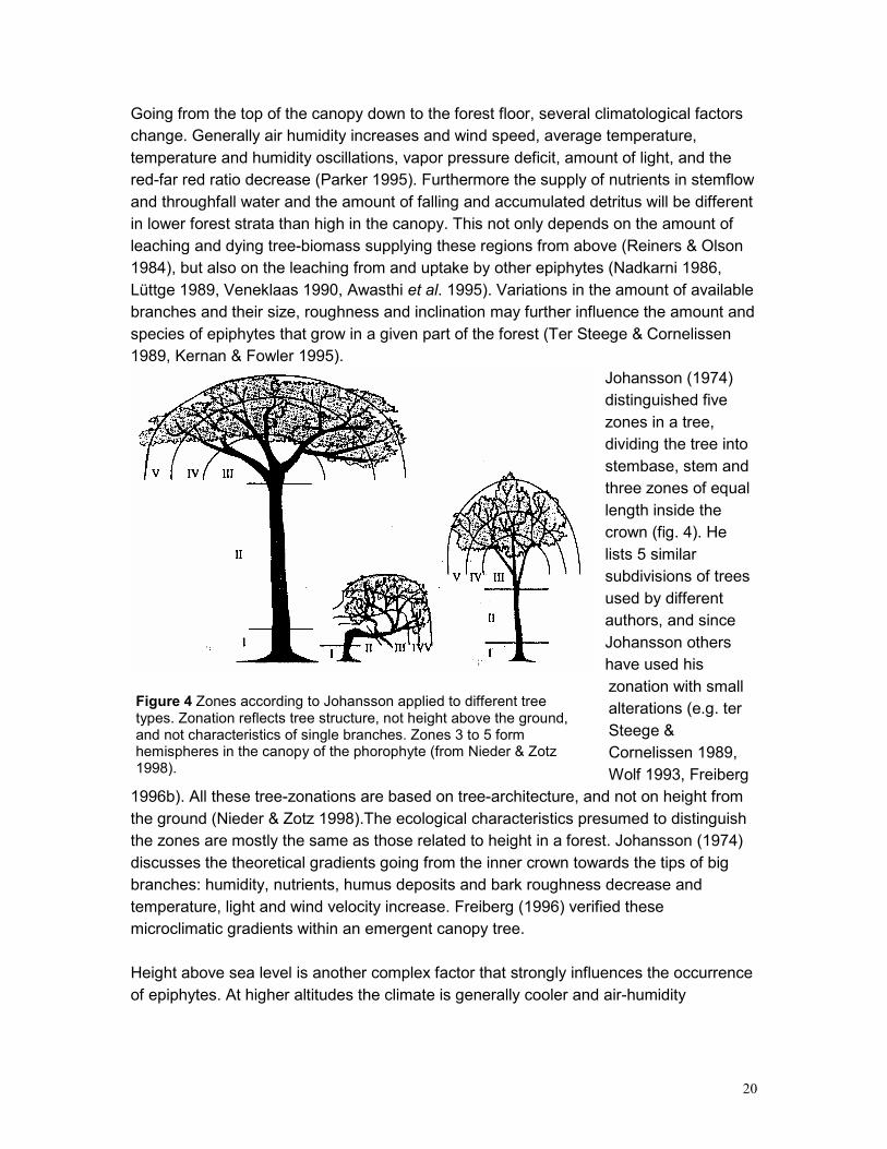
Johansson (1974)
distinguished five
zones in a tree,
dividing the tree into
stembase, stem and
three zones of equal
length inside the
crown (fig. 4). He
lists 5 similar
subdivisions of trees
used by different
authors, and since
Johansson others
have used his
zonation with small
alterations (e.g. ter
Steege &
Cornelissen 1989,
Wolf 1993, Freiberg
1996b). All these tree-zonations are based on tree-architecture, and not on height from
the ground (Nieder & Zotz 1998).The ecological characteristics presumed to distinguish
the zones are mostly the same as those related to height in a forest. Johansson (1974)
discusses the theoretical gradients going from the inner crown towards the tips of big
branches: humidity, nutrients, humus deposits and bark roughness decrease and
temperature, light and wind velocity increase. Freiberg (1996) verified these
microclimatic gradients within an emergent canopy tree.
Height above sea level is another complex factor that strongly influences the occurrence
of epiphytes. At higher altitudes the climate is generally cooler and air-humidity
Figure 4 Zones according to Johansson applied to different tree types. Zonation reflects tree structure, not height above the ground, and not characteristics of single branches. Zones 3 to 5 form hemispheres in the canopy of the phorophyte (from Nieder & Zotz 1998).
21
increases (Wolf 1993). Forests change in structure and tree species composition at
increasing altitude, providing different quantities and qualities of substrate to epiphytes.
These differences in structure do not only occur between different altitudes, but also
between different forests at the same altitude. Secondary forests can provide a wide
range of forest structures, depending on their age, position and history. Such forests can
be very suitable for studying the influence of the above-mentioned environmental factors
on epiphytes, independent of altitude. However, when forests of different ages are
compared, the difference can also be due to the varying amount of time that has been
available for recolonization and growth. For studying environmental influences this
problem can be overcome by comparing different types of even aged secondary
vegetation.
Apart from the growing conditions the supply of propagules is an important factor
determining the distribution of epiphytes. When species seem ecologically equal, it may
in fact be the most important factor (Benzing 1981b, Yeaton & Gladstone 1982).
Obviously epiphytes do not have a seedbank in the soil, so in regrowing forests the first
epiphytes must arrive from the surrounding vegetation. Remnant forest fragments, even
single trees, can be an important reservoir for epiphyte diversity and a source for seeds
in regrowing forest. Isolated remnants in Mexico have been shown to have a high
epiphytic species richness, similar to that of trees in undisturbed forests (Hietz-Seifert et
al. 1996), and to contain in part species that occur also in undisturbed forests (Williams-
Linera et al. 1995).
Barkman (1958) summarizes the factors that are important for epiphyte establishment as
follows: “1. accessibility (can diaspores of the species reach the locality?), 2. priority (is
the habitat already occupied by other species?), 3. environment (does it enable the
species to germinate and grow?), 4. competition (can the species withstand competition
of other species already present or coming shortly afterwards?).” For vascular epiphytes
the first and third factor are the most important, factor 2 and 4 applying mostly to mat-
forming bryophytes (Barkman 1958, Wolf 1993).
In the present study the spatial distribution of angiosperm epiphytes was studied, in an
attempt to quantify ‘accessibility’ and ‘environment’ in an open, heterogenous secondary
upper montane forest. The study was also an exploration of methods for quantitatively
describing epiphyte distributions.
An additional research objective was to study the relation between bromeliad
morphology and some environmental factors. Possible relations between environment
and bromeliad color and shape, as described in chapter 1.4, were investigated for the
species in the study area.

22
3 Study area
The study area is situated at 3000 meters
above sea level at the west side of the
Cordillera Central, near the town Santa
Rosa de Cabal in the province Risaralda,
Colombia (ca. N 04 50'17'', W 75 30'14'')
(fig. 5). The study site is situated close to the
Parque Nacional Los Nevados, containing
several more or less dormant, snow-capped
volcanoes, some over 5000 meter in height.
Soils in the area are of volcanic origin.
The climate at 3000 m is moist and cool, but
temperatures rarely, if ever, drop below
zero. Wolf (1993) has recorded relative air
humidity being close to 95% most of the
time, with temperatures between 5 and 10
°C. Usually clouds move upwards from the
valley in the morning, causing rain early in the afternoon. Sunny periods usually occur in
the morning and later in the afternoon, after the clouds have moved away again (pers.
obs.). The climate is relatively constant throughout the year. Two periods with higher
rainfall can be distinguished, one around May and one around October, coinciding with
the passing of the Intertropical Convergence Zone (Veneklaas 1990). This pattern has
been disturbed the last few years, probably through the influence of the climatological
phenomena El Niño and La Niña. The forest line is quite high in the region: the paramo
vegetation starts at ca. 3700 m.
Human disturbance and the natural occurrence of landslides on steep slopes make the
area a mosaic of different stages of secondary growth. This study was conducted in a
20-year old secondary growth shrub-vegetation or very open forest (fig. 6) on deserted
pastureland. This area was selected because of its accessibility, its high abundance of
vascular epiphytes, low stature and heterogeneity. The low stature was important to
avoid the necessity to climb trees, which costs a lot of time and which is not very safe in
many higher secondary forests, because trees are rather thin. Heterogeneity was
needed for comparing different forest structures.
All plots were situated on the top of a wide ridge, running approximately East-West,
down from the main Central Cordillera chain. The area was totally surrounded by forests,
which also were secondary or disturbed patches, but generally denser and higher, and
probably older, than the forest in the study area. Several tall remnant trees (up to 23 m
high), containing big bromeliad clusters, were present in the study area.
The most abundant shrubs and tree species in the study area are the pioneer shrub
Tibouchina grossa (Melastomataceae), shrubs of Escallonia cf. myrtilloides L.F.
Figure 5 Position of study area: Santa Rosa de Cabal, Central Cordillera, Colombia.

23
(Saxifragaceae), the trees Clethra sp.,
three Miconia-species
(Melastomataceae) and the bamboo
Chusquea sp. (Poaceae). Two
Weinmannia species (Cunoniaceae) are
present with mostly young trees up to
two meters in height and a DBH around
1cm.
Weinmannia-species and Chusquea
are characteristic for forests at this
altitude: Chusquea scandentis-
Weinmannion rollottii alliance, recorded
from 2820-3250 m (Wolf 1993).
Escallonia myrtilloides is more
characteristic for forests near the forest
line, which are more open and of lower
stature (Cleef et al. in prep. in Wolf
1993), but has also been found in
primary and secondary forests at 3100
m, as have several Miconia species
(Cavalier 1995).
The study area is clearly distinct from
some nearby patches of regenerating
forest, even though they have been
abandoned approximately at the same
time. When the area was abandoned
some areas grew tall (15-20 m)
homogenous forests with little undergrowth, while other parts, like the study-area,
developed an open, heterogeneous shrub vegetation, with trees up to 8 meters (fig. 6)
(excluding some remnant trees still present). This difference is probably due mainly to a
different land use history. The soil in the study area has probably been compacted by
the grazing of cattle and is now relatively impermeable, leaving a wet surface where
peatmosses (Sphagnum) flourish. The taller homogenous forest has probably not been
used intensively after clearcutting (Hanke 1999), so the regrowth has been easier.
Geomorphology is another factor that may contribute to the difference between the two
forests. The (locally) relatively flat character of the study area adds to the possibilities for
stagnation of water and thus Sphagnum-growth. The other forest is situated on steeper
slopes, so water can run off easier. The distribution of Bromeliaceae in this forest has
been studied by Hanke (1999).
Figure 6 Example of a common forest structure in the study area, in this case in plot B. Arrows point out some bromeliads.

24
At this stage it is difficult to tell whether the peatmosses in the study area will eventually
'suffocate' the shrubs and trees, or whether the trees will overshadow the Sphagnum
and development will go towards a cloud forest vegetation.

25
4 Method
4.1 Fieldwork
All angiosperm epiphytes were sampled in eleven 5x5-m plots (plots A-K). The following
criteria were used for selection of the plots: at least two trees over 4 m high should be
present within the plot; the ground should be more or less level; there should not be a
track or other disturbance inside the plot; there should not be more than 5 m² of bamboo
inside the plot (this grows very fast and would alter the circumstances rapidly, so that the
epiphytes might not yet have reacted to it).
Within the plots all angiosperm epiphytes (and some terrestrial specimens of generally
epiphytic species) were mapped, giving them three co-ordinates: z for height and x and y
for horizontal position within the plot. Growing sites and plants were noted in separate
tables, to avoid redundancy of data where several epiphytes were growing at the same
position. For each growing site, the branch-size and -inclination, the exposition and
position of the epiphyte on the branch (N/E/S/W-side of the branch)(top/side/bottom) and
the surrounding epiphytic vegetation (mosses and lichens) were described. Every
epiphyte was described by species, size, viability (alive/poor/dead) and life-stage
(seedling/ juvenile/ small clone-shoot/ vegetative adult/ flowering/ fruiting). Bromeliaceae
over 5 cm had three sizes taken: vertical distance and horizontal distance at the top and
the base of the plant. Smaller bromeliads and species of the other families only had their
vertical size taken. Of two bromeliad species (Racinaea tetrantha and Tillandsia
compacta) the color of the leaves was recorded and light was measured (W/m²), using a
Mavolux digital photometer (Gossen instruments).
Trees and shrubs over 2 m were mapped and described: species, position of stem-base
(xy-co-ordinates), height, DBH, total branch length per thickness-class (1-2, 2-5, 5-10,
>10 cm diameter) and epiphyte-cover (cryptogams) in three vertical zones (0-1, 1-3 and
>3 m). Taxa were identified by comparison to herbarium material at the Universidad de
Antioquia, Medellín. Vouchers of the species have been deposited at the same
herbarium.
A ground-projection of the tree-crowns was drawn in a 5x5 grid representing the plot.
Additional information on crowns was their height, thickness (vertical distance from top
to bottom) and denseness (relative measure for the amount of branches and leaves per
unit volume: open, medium or dense). Undergrowth was described in a grid of 1x1-m
blocks. In the plot, plus a 1-m strip around it, the average height, denseness and
species-composition of the undergrowth were recorded per block.
In plots that were not level, the slope was measured with the aid of a little level on a
rope. This was used to make a horizontal connection between different points around
the plot border, including the corners, after which the height difference could be
determined.

26
Temperature (in C°) and relative humidity
(RH, in %) were measured in every plot at
0.5, 2 and 4 meters above the ground, for
3 days, starting at 12 am, with a recording
every 2:24 minutes. Two plots were
sampled per 3-day period, and an open
reference location was measured every
time, at 2 meters from the ground. The
measurements were recorded by
Stowaway dataloggers (Onset Corp.),
which were hung up inside white wooden
weather-houses (fig.7), constructed
especially for this purpose after a design
used by Wolf (1993). The pairs of plots
measured in the same week were: A-C, B
alone, D-E, F-G, H-K and I-J.
The position of the plots relative to each
other and the nearest remnant trees was
determined using a 50 meter measuring
tape, a compass and clinometer. The
clinometer was used to calculate
distances to remnants. First the length of
a trunk-portion was calculated from the
angle observed between the top and a
salient feature on the trunk, from a known
distance. Then the angle between the same points was taken from the plot, and this was
used to calculate the distance.
4.2 Data analysis
Recording the exact co-ordinates of all epiphytes and other features in the plots allowed
for the use of geographical information systems (GIS) in the analysis, and also for some
of the more powerful statistical distance methods, like the K function (Cressie 1993,
Young & Young 1998).
4.2.1 GIS
Data were entered in the GIS-package ArcInfo, and analyses were carried out using
both this program and the related ArcView. This is the first time that a GIS has been
used to study the spatial distribution of epiphytes. GIS-software is designed for 2-
dimensional data while the epiphyte data was recorded in three dimensions, so some
special operations had to be used to be able to make some of the analyses.
Figure 7 The reference dataloggers in their house.
27
GIS pre-processing
Most of the time and work needed for the use of a GIS for any kind of data, is involved
with the construction of the spatial database: the pre-processing phase. Once the
database works well, analysis can be relatively simple. This certainly applied to this
study. Figure 9 shows the steps of data handling in a general GIS approach.
The drawings of the treecrown-projections were scanned and digitized. The overlap-
areas, forming closed shapes and hence separate polygons in the GIS topology, were
combined to make a region representing an individual crown, to which the attributes
(height, denseness, etc.) were assigned.
A sloping ground level was represented by a digital elevation model (DEM), which was
an interpolation between the height-points measured around the plot borders. This DEM
was then used to correct the height of other features. This gives a more correct
representation of the spatial positions then height from the ground, which does not
accurately describe the mutual positions if the ground is not level.
After correction of the undergrowth-height for the ground height, a DEM was made for
the upper boundary of the undergrowth by interpolation of the height between the
centers of the 1x1-m blocks.
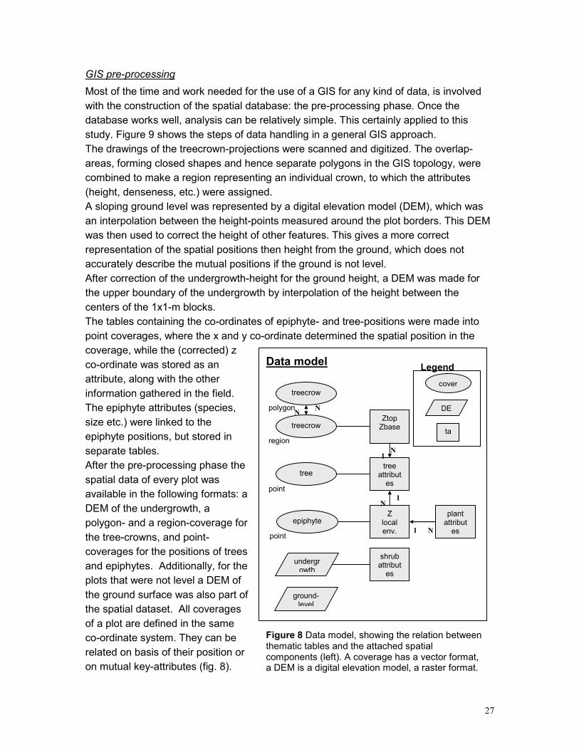
The tables containing the co-ordinates of epiphyte- and tree-positions were made into
point coverages, where the x and y co-ordinate determined the spatial position in the
coverage, while the (corrected) z
co-ordinate was stored as an
attribute, along with the other
information gathered in the field.
The epiphyte attributes (species,
size etc.) were linked to the
epiphyte positions, but stored in
separate tables.
After the pre-processing phase the
spatial data of every plot was
available in the following formats: a
DEM of the undergrowth, a
polygon- and a region-coverage for
the tree-crowns, and point-
coverages for the positions of trees
and epiphytes. Additionally, for the
plots that were not level a DEM of
the ground surface was also part of
the spatial dataset. All coverages
of a plot are defined in the same
co-ordinate system. They can be
related on basis of their position or
on mutual key-attributes (fig. 8).
Figure 8 Data model, showing the relation between thematic tables and the attached spatial components (left). A coverage has a vector format, a DEM is a digital elevation model, a raster format.
ground- level
epiphyte
treecrowns
Z local env.
undergrowth
Ztop Zbase
tree attributes
tree
plant attributes
shrub attributes
Data model
N
1
1 N
1
N
cover
DE
tabl
Legend
treecrowns
polygon
region
point
point
N N

28
Figure 9 Scheme of the process of data handling, including the use of a GIS.
ground-
level
epiphyte
treecrowns
Z
local env.
attributes
undergrowth
Ztop
Zbase
tree
attributestree
plant
attributes
shrub
attributes
Data model
N
1
1N
1
N
coverage
DEM
table
Legend
GIS-database
(pre-) processing
raw data
data model concept real world
presentation
data acquisition
2385821166311024467452N =
Dendrop. spec
Lor. spec1
Orchid spec5
Orchid spec1
Orchid specs
Brom. specs
R. penlandii
T. spec1
T. compacta
R. tetrantha
distance under crown-top (m)
5
4
3
2
1
0
x y z a b
analysis z a b
29
GIS-analysis
The positions of the epiphytes relative to the crowns were determined by means of an
overlay operation in ArcView. To be able to do this, it was first necessary to distinguish
the highest and lowest crown above each epiphyte, out of all the overlapping crowns
above some of them. Then epiphytes were assigned the heights of the top of the highest
and the bottom of the lowest crown straight above or beneath it. Also the distances
between epiphytes and the undergrowth-DEM were determined.
The crown-coverage provided area-values, the cover on the ground projection in m2, for
all the crowns. These, combined with the height and thickness of the crowns, were used
to determine the crown-volumes per plot and per height-layer. The undergrowth-DEM
was used to determine the volume of undergrowth per height-layer. These one-meter
thick height-layers were used in the analysis to get a grip on the vertical variation in the
amount of substrate within plots.
Several possibilities for presenting the spatial data graphically, as maps, were tried out
(appendix II)
More detailed information on the GIS-processing will be available in a report for the
Laboratory of Geo-Information science and Remote Sensing (GIRS), Wageningen
Agricultural University (Bader et al. in prep).
4.2.2 Spatial point pattern
To analyze the spatial pattern of the epiphytes the K(h) and L(h) functions were used
(Young & Young 1998, Cressie 1993). These require a complete map of points, and can
effectively summarize spatial dependence over a wide range of scales (Cressie 1993).
The K function is based on the number of points within a given distance of each point.
By varying this ‘given distance’ (h), the scale at which the spatial pattern is expressed
changes as well. The K function is defined as follows:
K(h) = λ-1 E[number of other points within distance h of an arbitrary point] with h ≥ 0.
Where λ is the intensity or density of points within the plot. Division by the intensity
makes the measure independent of it, making it possible to compare patterns of different
densities.
As the plots of this study were rather small, a correction for the edges had to be made,
resulting in the K2(h)-function. In this function the number of points within a circle (radius
= h) is divided by the proportion of the circle that is situated inside the plot.
The values found are compared to a simulation envelope, which is constructed by 100
permutations of the function for completely random patterns with the specified amount of
points in the specified area. If the test value is within the simulation envelope, the pattern
does not deviate from complete spatial randomness (csr). If it is above it, the points are
clustered, if it is below it the point-spacing shows regularity. The L2(h)- function is an
30
adaptation of K2(h), centered around zero, with clustering when L2(h) is above the
simulation envelope and regularity when it is lower.
Calculations were made using ‘Ecostat’-software (Young & Young 1998)a. Unfortunately
it is not possible in either to analyze a three-dimensional pattern directly, although the
formula is applicable for 3D-point patterns as well as those in 2 dimensions. The
intensity would however need to be calculated for a cube or cylinder rather than a
rectangle or circle, and the distances between points with three co-ordinates. It would be
interesting for future research to implement the possibility for making these calculations
in statistical software, like Ecostat. In this research however, a triple two-dimensional
analysis was run, looking at the xy- xz- and yz-plane separately.
Clustering of epiphytes was of course expected, because the substrate has a strongly
clustered distribution. However, a comparison within plots could reveal something about
extra clustering of epiphyte species. The level of clustering of Racinaea tetrantha was
compared to that of all epiphytes together, and R. tetrantha adults and juveniles were
compared where numbers were sufficient to allow for it.
4.2.3 Climatic data
The datalogger-output, consisting of ca. 1810 records with the time and the temperature-
or RH -values, was condensed to the following measures (taking the 3 days together):
mean, standard deviation, minimum and maximum, for temperature and RH. To be able
to compare the outcome in different weeks, these values were standardized by
subtracting the reference values for the corresponding weeks. Climate-differences
between heights were studied visually and tested using a Kruskall Wallis test (KW).
4.2.4 Height distribution
Height distributions of several epiphyte-species were tested with Kolmogorov Smirnov's
(KS) test for normality. They were not normally distributed and could not be transformed
to confirm to Anova-conventions. Therefor differences between height distributions of
different epiphyte-species and –families were tested by means of the non-parametric
Kruskall-Wallis test. Apart from height from the ground, several other ‘height’-measures
were tested: distance from the undergrowth, distance from the base of the crown and
distance from the top of the crown, straight up or down from the epiphyte. These
alternative ‘height’-measures were compared between epiphyte-groups using a Kruskall-
Wallis test. Their distributions were tested with KS test for normality, and test statistics
were compared to those for height from the ground.
The amount of substrate on different heights was estimated by calculating the volume of
crown or undergrowth in different height layers (1 meter thick).
a Another program that can make these calculations is ‘Splus’, but this program also cannot make 3D
calculations for the K function.
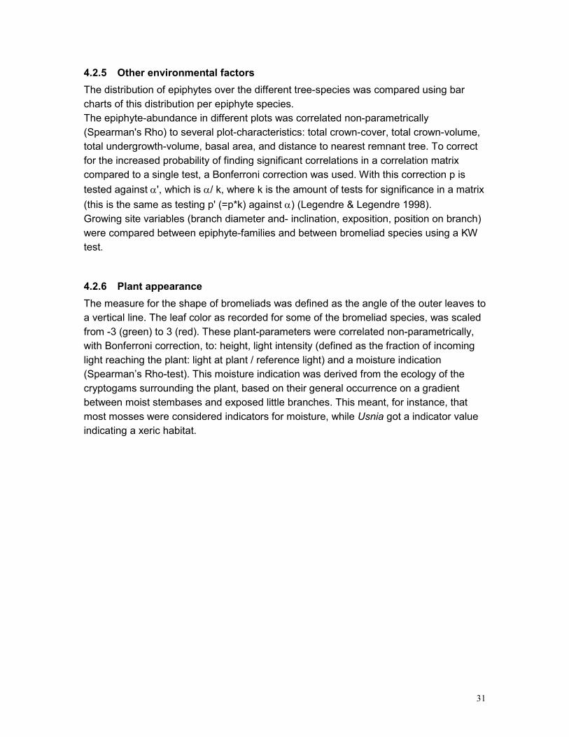
31
4.2.5 Other environmental factors
The distribution of epiphytes over the different tree-species was compared using bar
charts of this distribution per epiphyte species.
The epiphyte-abundance in different plots was correlated non-parametrically
(Spearman's Rho) to several plot-characteristics: total crown-cover, total crown-volume,
total undergrowth-volume, basal area, and distance to nearest remnant tree. To correct
for the increased probability of finding significant correlations in a correlation matrix
compared to a single test, a Bonferroni correction was used. With this correction p is
tested against α', which is α/ k, where k is the amount of tests for significance in a matrix
(this is the same as testing p' (=p*k) against α) (Legendre & Legendre 1998).
Growing site variables (branch diameter and- inclination, exposition, position on branch)
were compared between epiphyte-families and between bromeliad species using a KW
test.
4.2.6 Plant appearance
The measure for the shape of bromeliads was defined as the angle of the outer leaves to
a vertical line. The leaf color as recorded for some of the bromeliad species, was scaled
from -3 (green) to 3 (red). These plant-parameters were correlated non-parametrically,
with Bonferroni correction, to: height, light intensity (defined as the fraction of incoming
light reaching the plant: light at plant / reference light) and a moisture indication
(Spearman’s Rho-test). This moisture indication was derived from the ecology of the
cryptogams surrounding the plant, based on their general occurrence on a gradient
between moist stembases and exposed little branches. This meant, for instance, that
most mosses were considered indicators for moisture, while Usnia got a indicator value
indicating a xeric habitat.
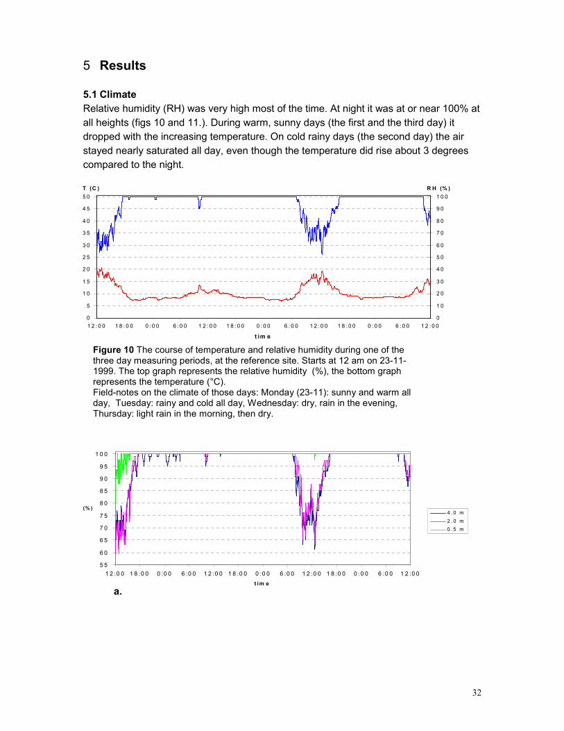
32
5 Results
5.1 Climate
Relative humidity (RH) was very high most of the time. At night it was at or near 100% at
all heights (figs 10 and 11.). During warm, sunny days (the first and the third day) it
dropped with the increasing temperature. On cold rainy days (the second day) the air
stayed nearly saturated all day, even though the temperature did rise about 3 degrees
compared to the night.
5 5
6 0
6 5
7 0
7 5
8 0
8 5
9 0
9 5
1 0 0
1 2 :0 0 1 8 :0 0 0 :0 0 6 :0 0 1 2 :0 0 1 8 :0 0 0 :0 0 6 :0 0 1 2 :0 0 1 8 :0 0 0 :0 0 6 :0 0 1 2 :0 0
t im e
R H (% )4 . 0 m
2 . 0 m
0 . 5 m
a.
0
5
1 0
1 5
2 0
2 5
3 0
3 5
4 0
4 5
5 0
1 2 :0 0 1 8 :0 0 0 :0 0 6 :0 0 1 2 : 0 0 1 8 : 0 0 0 :0 0 6 :0 0 1 2 :0 0 1 8 : 0 0 0 : 0 0 6 :0 0 1 2 :0 0
t im e
T (C )
0
1 0
2 0
3 0
4 0
5 0
6 0
7 0
8 0
9 0
1 0 0
R H (% )
Figure 10 The course of temperature and relative humidity during one of the three day measuring periods, at the reference site. Starts at 12 am on 23-11-1999. The top graph represents the relative humidity (%), the bottom graph represents the temperature (°C). Field-notes on the climate of those days: Monday (23-11): sunny and warm all day, Tuesday: rainy and cold all day, Wednesday: dry, rain in the evening, Thursday: light rain in the morning, then dry.

33
5
6
7
8
9
10
11
12
13
14
15
16
17
18
19
20
12 :00 18 :00 0 :00 6 :00 12 :00 18 :00 0 :00 6 :00 12 :00 18 :00 0 :00 6 :00 12 :00
t im e
T (C )
4 .0 m
2 .0 m
0 .5 m
b.
Figure 11 Course of the climate in plot H at three different heights during three days, starting at 12 am on 23-11-1999 (same period as figure 10). a.) Relative humidity (%). b.) Temperature (°C).
Average RH, as measured and after correction for the reference, differed significantly
between heights (KW, p < 0.001): it decreased with distance from the ground (fig. 12).
Maximum RH was always 100%, while minima differed significantly (p < 0.01), with
higher values at 0.5 meter. Variations in humidity through time were lower at 0.5 m than
at 2 and 4 m (p < 0.001)(fig. 13). In nearly all cases the average RH at every height in
the plots was higher than that at the open reference site (fig. 11b).
KJIHGFEDCBA
average RH (%)
101
100
99
98
97
96
95
94
93
92
height
0,5 m
2,0 m
4,0 m
KJIHGFEDCBA
average RH - ref. average (%)
6
5
4
3
2
1
0
-1
-2
height
0,5 m
2,0 m
4,0 m
a. b.
Figure 12 Average of relative humidity (%) over three days at three heights in the different plots (A, B, …, K). a.) RH measured. b.) difference between the average of the reference measurement and the average of the measurements in the plot.
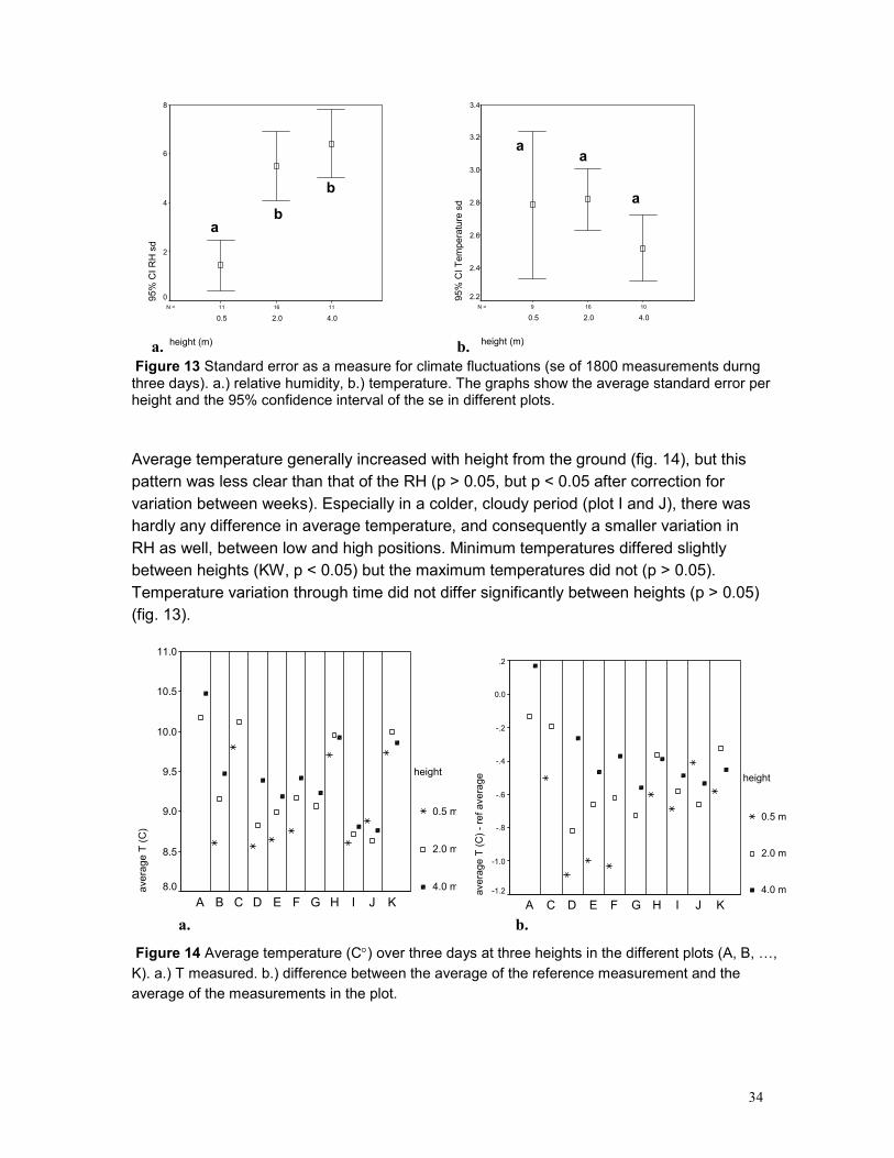
34
10169N =
height (m)
4.02.00.5
95% CI Temperature sd
3.4
3.2
3.0
2.8
2.6
2.4
2.2
111611N =
height (m)
4.02.00.5
95% CI RH sd
8
6
4
2
0
a. b.
Figure 13 Standard error as a measure for climate fluctuations (se of 1800 measurements durng three days). a.) relative humidity, b.) temperature. The graphs show the average standard error per height and the 95% confidence interval of the se in different plots.
Average temperature generally increased with height from the ground (fig. 14), but this
pattern was less clear than that of the RH (p > 0.05, but p < 0.05 after correction for
variation between weeks). Especially in a colder, cloudy period (plot I and J), there was
hardly any difference in average temperature, and consequently a smaller variation in
RH as well, between low and high positions. Minimum temperatures differed slightly
between heights (KW, p < 0.05) but the maximum temperatures did not (p > 0.05).
Temperature variation through time did not differ significantly between heights (p > 0.05)
(fig. 13).
KJIHGFEDCBA
average T (C)
11.0
10.5
10.0
9.5
9.0
8.5
8.0
height
0.5 m
2.0 m
4.0 m
KJIHGFEDCA
average T (C) - ref average
.2
0.0
-.2
-.4
-.6
-.8
-1.0
-1.2
height
0.5 m
2.0 m
4.0 m
a. b.
Figure 14 Average temperature (C°) over three days at three heights in the different plots (A, B, …,
K). a.) T measured. b.) difference between the average of the reference measurement and the
average of the measurements in the plot.
a b
b
a a
a

35
5.2 Epiphyte species
Nearly all epiphytes encountered belonged to three families: Bromeliaceae, Orchidaceae
and Loranthaceae. An occasional Peperomia-like epiphyte was found and some
unidentified plants that were probably just accidental epiphytes growing in some detritus
on the tree. This ‘rest’ group only contained 8 records and was excluded as a group from
most numerical analysis.
Bromeliaceae
Four species of Bromeliaceae
were found within the studied
plots (fig. 15): Racinaea tetrantha
(Ruiz & Pavon) M.A. Spencer &
L.B. Smith (formerly Tillandsia
tetrantha), Racinaea penlandii
(L.B. Smith) M.A. Spencer & L.B.
Smith (formerly Tillandsia
penlandii), Tillandsia compacta
Griseb., and an unidentified
Tillandsia-species (Tillandsia
sp.1). Ca. 96% of all
Bromeliaceae was identifiable to
one of these species. Some
seedlings and aberrant
specimens were classified
Bromeliaceae spp. Vriesea
capituligera was encountered in
the study area and Tillandsia
complanata in a fallen remnant
close by, but neither was found in
the studied plots. Vriesea,
Tillandsia and Racinaea are all
genera from the subfamily
Tillandsioideae, which typically
have plumed seeds.
Orchidaceae
Although many species of Orchidaceae were present in the study area, very few were
found flowering within the plots. Two species were found and recognized rather often,
but they were never found flowering. Both were probably species from the genus
Epidendrum, an exclusively epiphytic genus that contains 500 species (Kress 1989). The
species Orchidaceae sp.5 had green leaves of about 4 cm in length and a purple stem,
Figure 15 The three most common species of bromeliads found. From top to bottom: Racinaea tetrantha, Tillandsia compacta (both adults but not fully grown yet), and Tillandsia sp.1 (adult size).

36
about 5 mm in diameter, which had a woody appearance in bigger individuals.
Orchidaceae sp.1 had bigger leaves (up to 6 cm) and stem (diameter of 1 cm) and
generally grew rather tall, up to 1 meter, but did not seem to turn woody. Both species
formed clones. Orchidaceae sp.1 was always encountered in humus accumulations at
stem bases, with the roots hidden under a moss cover, while Orchidaceae sp.5 was truly
epiphytic. The roots of this species were found running up to a meter up or down the tree
trunk.
All other orchids were taken together as Orchidaceae spp., due to difficulties in
identifying and distinguishing the species and low abundance of many species. Some of
these species had pseudobulbs, others did not. The only orchid found flowering within
the plots was Frondaria caulescens, which was also added to the Orchidaceae spp.-
group on account of its low numbers.
Loranthaceae
At least two species of mistletoes were encountered. One was a Dendrophtora –species
(Loranthaceae). The other was probably a Loranthacea too, but has not been identified
to genus, and will be denoted as Loranthaceae sp.1.
The Dendrophtora sp. is a woody shrub up to about a meter tall. It has bright orange
leaves, about 10 cm in length, non-succulent and with an ovate shape. The other
species is smaller (up to ca. 40 cm) and not woody. The leaves are yellowish green, up
to 4 cm in length, lightly succulent and with a lanceolate shape. Both species have a
simple haustorium, without external runners. Both caused a thickening of the host
branch, which was more pronounced in the Dendrophtora. Many Loranthaceae are
pollinated by nectar-feeding birds (Reid et al. 1993), but although hummingbirds are
common in the area, no conspicuous flowers were observed in either species. Flowers
were small, with a color similar to that of the rest of the plant.
5.3 Epiphyte abundance
A total number of 1537 angiosperm epiphytes was recorded in the 11 plots. This number
results from counting all ramets. The number of genets (genetic individuals) is somewhat
lower, because the 1108 bromeliad ramets were contained in 894 dense clusters. These
clusters will from now on be called genets or clones, although some of them might be
formed by more than one genetic individuala. These ‘genets’ ranged from big clones (one
extreme cluster contained 27 ramets) to tiny single seedlings (table 1).
The Loranthaceae were represented by 73 individuals, and the Orchidaceae by 364
ramets, a few of which were parts of a clone. The demographic structure of the
populations differs markedly between some species.
a An alternative term could be ‘stand’: a compact group of plants, well-separated from conspecifics (Sanford 1968, in Bøgh 1992).
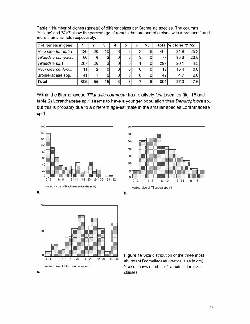
37
Table 1 Number of clones (genets) of different sizes per Bromeliad species. The columns ‘%clone’ and ‘%>2’ show the percentage of ramets that are part of a clone with more than 1 and more than 2 ramets respectively.
# of ramets in genet 1 2 3 4 5 6 >6 total % clone % >2
Racinaea tetrantha 420 20 10 3 3 3 6 465 31.8 25.3
Tillandsia compacta 66 6 2 0 0 3 0 77 35.3 23.5
Tillandsia sp.1 267 26 3 0 0 1 0 297 20.1 4.5
Racinaea penlandii 11 2 0 0 0 0 0 13 15.4 0.0
Bromeliaceae spp. 41 1 0 0 0 0 0 42 4.7 0.0
Total 805 55 15 3 3 7 6 894 27.3 17.6
Within the Bromeliaceae Tillandsia compacta has relatively few juveniles (fig. 16 and
table 2) Loranthaceae sp.1 seems to have a younger population than Dendrophtora sp.,
but this is probably due to a different age-estimate in the smaller species Loranthaceae
sp.1.
vertical size of Racinaea tetrantha (cm)
30 - 3224 - 2618 - 2012 - 146 - 80 - 2
160
140
120
100
80
60
40
20
0
a. vertical size of Tillandsia spec.1(cm)
16 - 1812 - 148 - 104 - 60 - 2
70
60
50
40
30
20
10
0
b.
vertical size of Tillandsia compacta(cm)
40 - 4432 - 3624 - 2816 - 208 - 120 - 4
20
10
0
c.
Figure 16 Size distribution of the three most
abundant Bromeliaceae (vertical size in cm).
Y-axis shows number of ramets in the size
classes.

38
Table 2 Number of epiphyte-ramets found, of different species at different life-stages . It should be noted that the counts of seedlings probably give an under-estimation of the number of seedlings actually present, because the tiny seedlings are easily overlooked. The seedlings, being ca. 5 mm long and light green, could not be determined to species. Clonejuv = small ramet growing from a clone. Juvenile = small individual (judged per species) without floral structures. Adult = non-flowering adult. (Past) flowering = flowering, fruiting or with old fruit capsules.
Lifestage: seedling clonejuv juvenile adult (past)
flowering total
Racinaea tetrantha 1 14 386 177 38 616
Tillandsia compacta 0 4 21 75 2 102
Tillandsia sp.1 0 0 252 82 0 334
Racinaea penlandii 0 0 3 9 1 13
Bromeliaceae spp. 22 0 19 2 0 43
Rest 0 0 7 1 0 8
Orchidaceae spp. 0 0 172 49 10 231
Orchidaceae sp.1 0 0 12 12 0 24
Orchidaceae sp.5 0 1 55 37 0 93
Loranthaceae spp. 0 0 9 2 1 12
Loranthaceae sp.1 0 0 16 1 4 21
Dendrophtora sp. 0 0 6 20 14 40
Total 23 19 958 467 70 1537
5.4 Height distribution
There is an optimum height for epiphyte occurrence, which lies around 1.8 meter from
the ground (fig.
17). The
distribution is
somewhat
stretched to the
right because of
some higher trees,
and therefor not
normal, and the
mean is not equal
to the optimum: the
mean is 2.15 meter
(std.dev. = 1.18).
The separate
species also show
an optimum, which
is logically is less
clear for the
species with lower abundance (appendix III).
Figure 17 Histogram of the height distribution of epiphytes, all species taken together.
Z (ALT), height above the ground in m
7,06,56,05,55,04,54,03,53,02,52,01,51,0,50,0
Height distribution of all epiphytes in all plots.
Frequency
250
200
150
100
50
0
Std. Dev = 1,18
Mean = 2,2
N = 1537,00

39
422193242294213334102617N =
Dendrop. spec
Lor. spec1
Orchid spec5
Orchid spec1
Orchid specs
Brom. specs
R. penlandii
T. spec1
T. compacta
R. tetrantha
height above the ground (m)
5
4
3
2
1
0
The average height of epiphytes from the undergrowth was 0.8 meter (std. dev. = 1.3),
and the average distance under crowns 1 meter under the crown base (std. dev. = 1.7)
and 2.8 meter under the crown-top (std. dev. = 1.6). Epiphytes were not normally
distributed in any of these measures, although these distributions approached normality
a bit more than that for height from the ground (K-S Z =2 or 3, instead of 5). The
distributions of the species separately did usually have a somewhat more normal
distribution for the alternative measures than they had for height from the ground, but
these are still hardly ever normal. The standard deviation (e.g. the variation) is higher
for the alternative measures than for the height from the ground, for all epiphytes
together as well as for the separate species (appendixIV).
Epiphyte species and
families differ
significantly in their
height distribution (KW, p
< 0.001 for both). The
Orchidaceae as a family
grow lowest in the forest
and the Loranthaceae
grow at higher positions
(appendix III). Two
epiphyte species are
rather extreme compared
to the rest; Dendrophtora
sp. grows higher and
Orchidaceae sp.1 grows
lower than the average
(fig. 18). Without these
species the difference
between species’ height distribution is still significant. However, the differences between
epiphyte species as detected by the KW-test, do not show up very convincingly in figure
18, except for the two extreme species. All other species have their optimum around 2
meter.
Whether height from the ground or the alternative height measures are tested, the
distributions of epiphytes-species and -families always differ significantly (always p <
0.01) (appendix V). When comparing Bromeliad-species only, the differences are not
significant when looking at the distance from the top of the crown (p>0.05), but for the
other measures they are (p < 0.001).
The height distribution of epiphytes does differ considerably between plots. In most plots
it is just below 2 meter, but in plot B, C and K the average is higher (around 2.2, 3.2 and
2.7 m respectively), while plot H has an average around 1.2 m (but very few epiphytes:
Figure 18 Mean height and 95% confidence interval per epiphyte species.

40
26) (appendix IV). Height above the undergrowth is even more variable, as are distance
under bottom and top of the crown (appendix IV). Epiphyte numbers are lower for the
latter two measures, because epiphytes that are not underneath any crown are not
counted; plot F is not shown, for the same reason.
5.5 Spatial point pattern
In some plots the K- and L-functions of the spatial distribution of the epiphytes could not
be calculated or interpreted. When epiphyte numbers were low, as was often the case
when taking Racinaea tetrantha separately, the simulation envelope is very wide and
irregular and the K- and L-graphs are also irregular. So for very low numbers these
graphs are not very valuable. The plotted L-functions can be found in appendix VI.
Two plots contained more epiphytes than the Ecostat software could handle, so in these
plots distributions were not analyzed for all epiphytes together but only for Racinaea
tetrantha.
Epiphytes have a clustered distribution in all plots and from all angles (in xy-, xz- and yz-
plane), though in some cases there is no deviance from ‘complete spatial randomness’
at bigger h.
On the xy-projection clustering is strongest at a small scale (small h) and decreases
when expanding the distance-circle (h) in most plots, though in some the difference is
slight, or based on very low numbers. Only in one plot does the measure of clustering
rise at bigger distances. On the contrary, on the xz- and yz-projections clustering
increases in nearly all cases with increasing h.
The distribution of R. tetrantha is sometimes more and sometimes less strongly
clustered than that of all epiphytes together. R. tetrantha juveniles are more clustered
than the adults of the same species in those cases where there are enough juveniles to
allow for such a comparison, which are only two plots.
5.6 Phorophytes
Nine tree species (or high shrubs) were regularly found in the plots. These were, in
decreasing abundance: Miconia squamulosa (Melastomataceae), Clethra sp.
(Clethraceae), Miconia thaezans (Melastomataceae), Weinmannia pubescens
(Cunoniaceae), Escallonia myrtilloides (Saxifragaceae), Miconia pergamentacea
(Melastomataceae), Tibouchina grossa (Melastomataceae), Weinmannia sp.
(Cunoniaceae), and Hedyosmum sp. (Chloranthaceae). Both Weinmannia species
occured mostly as very young trees of ca. 2 m tall.
There was also a considerable amount of dead trees, mostly present as stems only.
Some rare and/or unidentified species of shrubs (among which Disterigma acuminata
(H.B.K.)) Ndzu (Ericaceae), a Ericaceae sp., a Melastomataceae sp. and a shrub with
big thorns and small succulent leaves) were found higher than 2 m and registered as
phorophytes.
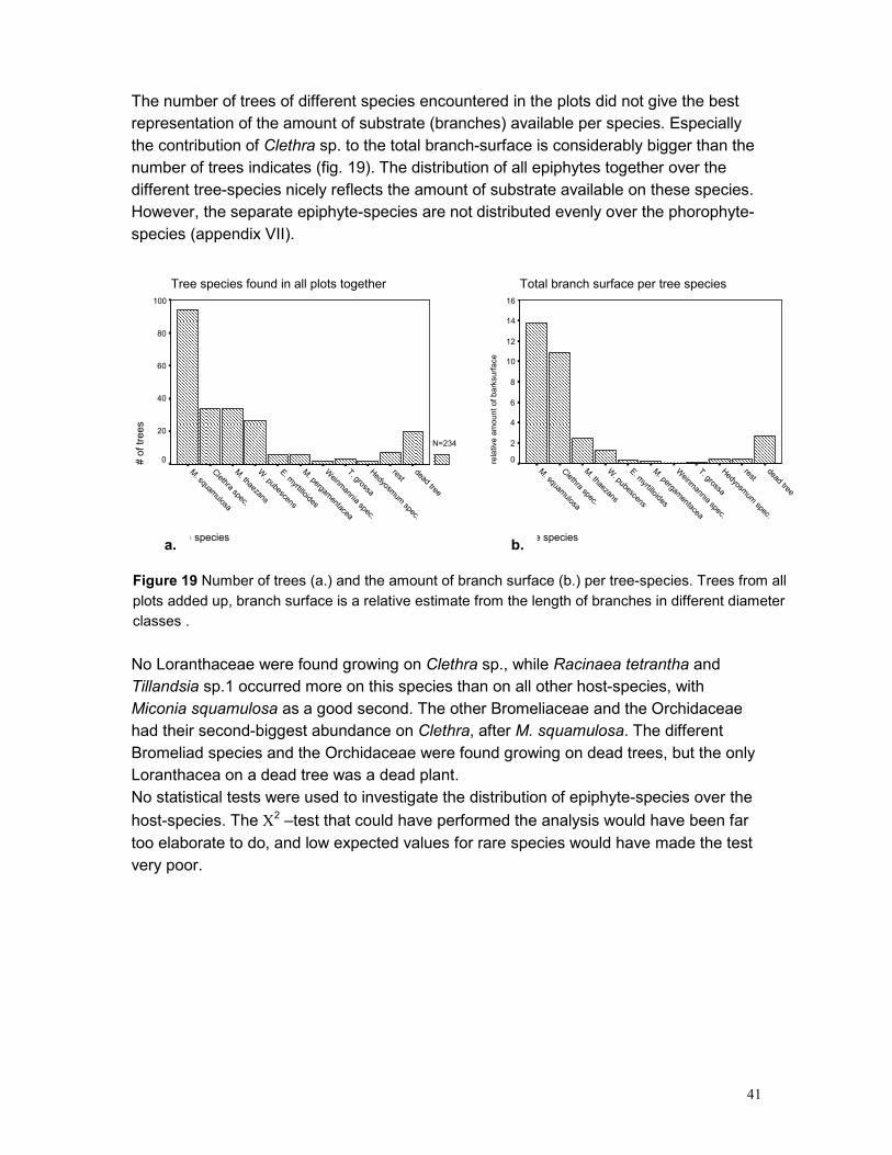
41
The number of trees of different species encountered in the plots did not give the best
representation of the amount of substrate (branches) available per species. Especially
the contribution of Clethra sp. to the total branch-surface is considerably bigger than the
number of trees indicates (fig. 19). The distribution of all epiphytes together over the
different tree-species nicely reflects the amount of substrate available on these species.
However, the separate epiphyte-species are not distributed evenly over the phorophyte-
species (appendix VII).
Total branch surface per tree species
Tree species
dead tree
restHedyosm
um spec.
T. grossa
Weinm
annia spec.
M. pergam
entacea
E. myrtilloides
W. pubescens
M. thaezans
Clethra spec.
M. squam
ulosa
relative amount of barksurface
16
14
12
10
8
6
4
2
0
Tree species found in all plots together
Tree species
dead tree
restHedyosm
um spec.
T. grossa
Weinm
annia spec.
M. pergam
entacea
E. myrtilloides
W. pubescens
M. thaezans
Clethra spec.
M. squam
ulosa
# of trees
100
80
60
40
20
0
N=234
a. b.
Figure 19 Number of trees (a.) and the amount of branch surface (b.) per tree-species. Trees from all
plots added up, branch surface is a relative estimate from the length of branches in different diameter
classes .
No Loranthaceae were found growing on Clethra sp., while Racinaea tetrantha and
Tillandsia sp.1 occurred more on this species than on all other host-species, with
Miconia squamulosa as a good second. The other Bromeliaceae and the Orchidaceae
had their second-biggest abundance on Clethra, after M. squamulosa. The different
Bromeliad species and the Orchidaceae were found growing on dead trees, but the only
Loranthacea on a dead tree was a dead plant.
No statistical tests were used to investigate the distribution of epiphyte-species over the
host-species. The Χ2 –test that could have performed the analysis would have been far
too elaborate to do, and low expected values for rare species would have made the test
very poor.
42
5.7 Plots
No correlation was found between any of the plot variables and the number of epiphytes
per plot (p' > 0.05). (table 3).
Table 3 Correlations between several plot-variables and the amount of epiphytes found in each plot (no significant correlations at the .05/15 or .01/15 level, the Bonferroni-corrected significance levels).
Spearman's Rho
(N = 11)
Number of
epiphytes
Crown-
cover (m2)
Volume of
crowns
(m3)
Volume of
undergrowt
h (m3)
Basal area
(cm2)
Cor. Coef. 1.000 .506 .114 .647* .761** Number of
Epiphytes Sig. (2-t) . .113 .739 .031 .007
Cor. Coef. .506 1.000 .427 .327 .636* Crowncover (m2)
Sig. (2-t) .113 . .190 .326 .035
Cor. Coef. .114 .427 1.000 .036 .227 Volume of crowns
(m3) Sig. (2-t) .739 .190 . .905 .502
Cor. Coef. .647 .327 .036 1.000 .591 Volume of
undergrowth (m3) Sig. (2-t) .031 .326 .915 . .056
Cor. Coef. .761 .636 .227 .591 1.000 Basal area (cm2)
Sig. (2-t) .007 .035 .502 .056 .
Cor. Coef. -.610 .000 .173 -.391 -.609 Distance to nearest
remnant (m) Sig. (2-t) .046 1.000 .612 .235 .047
5.8 Growing sites
Most epiphytes were found growing on branches of 2 to 5 cm diameter. Juveniles on
average occupy smaller branches than adults do. The trend as seen for adult and
juvenile Racinaea tetrantha (table 4) holds for all epiphytes. The correlation (Spearman’s
rho) between epiphyte size and branch size is significant at p< 0.001.
Table 4 Distribution of epiphytes over branches of different sizes. An occasional epiphyte was encountered growing on a leaf, on Frullania or on Usnia (='other').
branch class: <1 cm 1-2 cm 2-5 cm 5-10 cm >10 cm leaf other N
total all epiphytes 7.4% 17.8% 45.0% 24.2% 4.2% 1.1% 0.2% 1512
adult R. tetrantha 1.4% 8.5% 46.0% 36.6% 7.5% 0.0% 0.0% 213
juvenile R. tetrantha 14.5% 27.5% 37.0% 15.8% 1.0% 3.4% 0.8% 386
Most epiphytes (1079) were growing on the side of branches, including the sides of
vertical stems. Twice as many were found growing on the bottom-side of branches (275)
as on the top (143). For 37 individuals the position was not recorded. These will have
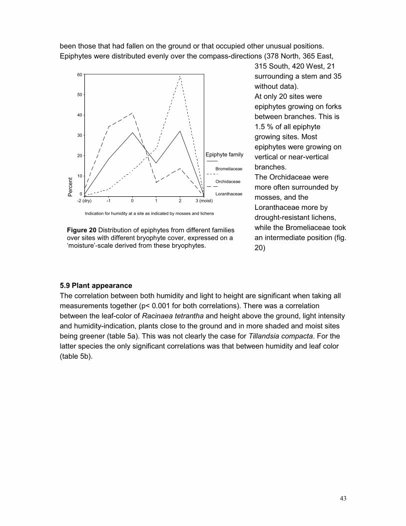
43
been those that had fallen on the ground or that occupied other unusual positions.
Epiphytes were distributed evenly over the compass-directions (378 North, 365 East,
315 South, 420 West, 21
surrounding a stem and 35
without data).
At only 20 sites were
epiphytes growing on forks
between branches. This is
1.5 % of all epiphyte
growing sites. Most
epiphytes were growing on
vertical or near-vertical
branches.
The Orchidaceae were
more often surrounded by
mosses, and the
Loranthaceae more by
drought-resistant lichens,
while the Bromeliaceae took
an intermediate position (fig.
20)
5.9 Plant appearance
The correlation between both humidity and light to height are significant when taking all
measurements together (p< 0.001 for both correlations). There was a correlation
between the leaf-color of Racinaea tetrantha and height above the ground, light intensity
and humidity-indication, plants close to the ground and in more shaded and moist sites
being greener (table 5a). This was not clearly the case for Tillandsia compacta. For the
latter species the only significant correlations was that between humidity and leaf color
(table 5b).
Indication for humidity at a site as indicated by mosses and lichens
3 (moist)210-1-2 (dry)
Percent
60
50
40
30
20
10
0
Epiphyte family
Bromeliaceae
Orchidaceae
Loranthaceae
Figure 20 Distribution of epiphytes from different families over sites with different bryophyte cover, expressed on a ‘moisture’-scale derived from these bryophytes.
44
Table 5 Spearman's rho correlation coefficients, for Racinaea tetrantha (a) and Tetrantha compacta (b), both for plants > 5 cm. Significance level with Bonferroni correction. Height in m above the ground. Light: light measured at plant/ reference outside, low value = much shading. Humidity: indication based on the presence of mosses and lichens, dry < 0, moist > 0. Color: ranging from green to red, green < 0, red > 0. Shape: angle of outermost leaf to vertical, big angle = wide plant. Size: vertical plant size in cm.
Height z light humidity color shape
height z Cor. Coef. 1.000 Sig. (2-t) .
N 315
light Cor. Coef. 0.501** 1.000 Sig. (2-t) 0.000 .
N 119 119
humidity Cor. Coef. -0.345** -0.231 1.000 Sig. (2-t) 0.000 0.011 .
N 315 119 315
color Cor. Coef. 0.388** 0.480** -0.248** 1.000 Sig. (2-t) 0.000 0.000 0.000 .
N 272 114 272 272
shape Cor. Coef. -0.140 -0.101 0.135 -0.258** 1.000 Sig. (2-t) 0.015 0.273 0.019 0.000 .
N 302 119 302 270 302
size Cor. Coef. 0.112 0.235 -0.016 0.014 0.371** Sig. (2-t) 0.046 0.010 0.782 0.815 0.000
N 315 119 315 272 302
**Correlation is significant at the .01/15 level (2-tailed). a. Racinaea tetrantha
Height z light humidity color shape
Height z Cor. Coef. 1.000
Sig. (2-t) .
N 91
Light Cor. Coef. 0.286 1.000
Sig. (2-t) 0.113 .
N 32 32
Humidity Cor. Coef. -0.041 -0.125 1.000
Sig. (2-t) 0.697 0.495 .
N 91 32 91
Color Cor. Coef. 0.285 0.387 -0.355* 1.000
Sig. (2-t) 0.011 0.031 0.001 .
N 79 31 79 79
Shape Cor. Coef. -0.171 0.228 0.200 -0.064 1.000
Sig. (2-t) 0.106 0.210 0.057 0.572 .
N 91 32 91 79 91
Size Cor. Coef. 0.143 0.021 0.222 -0.300 -0.067
Sig. (2-t) 0.175 0.909 0.035 0.007 0.531
N 91 32 91 79 91
* Correlation is significant at the .05/15 level (2-tailed).
b. Tillandsia compacta
45
6 Discussion
6.1 Climate
Air humidities recorded agree with the recordings of Wolf (1993), who also found very
high air humidity at this altitude. Hair extension in the hygrograph Wolf used is maximal
at 95% relative humidity, so humidities over 95% could not be recorded. With the
electronic dataloggers used in this study humidities up to 100% could be recorded, and
were recorded most of the time. The vertical climatic gradient found with these
measurements is in accordance with the trends that others have found for forest
climates (Freiberg 1997, Parker 1995).
6.2 Epiphyte species and abundance
Racinaea tetrantha, R. penlandii and Tillandsia compacta have a rather similar growth
form. They all have a tank and few trichomes. Tillandsia sp.1 has a narrower shape and
smaller tank and a high cover of trichomes on the entire leaves. This species could be
classified as an intermediate between tank- and atmospheric-absorbing trichome type in
the classification of Pittendrigh (1948), while the other three are typical tank-absorbing
trichome species. R. tetrantha and T. compacta have a C3-photosynthesis and a
chlorophyll concentration of 1.3 and 1.4 mg/g dry weight respectively (Martin 1994). No
information is available on the physiology of the other species.
The total number of epiphytes encountered in the study area is relatively high for this
region. Hanke (1999) encountered 200 bromeliad-ramets bigger than 5 cm (in 125
genets) in a 10x5 m transect that was less than a kilometer away from the plots studied
here. Although the eleven plots only have a surface 1.1 times that of Hanke’s transect,
4.5 times as many bromeliads bigger than 5 cm were recorded (907). Hanke worked in a
homogenous, relatively tall forest of approximately the same age as the area of this
study. In that forest Racinaea tetrantha was the most abundant species, followed by
Tillandsia compacta. The two other species found were not identified and also very low
in numbers (8 and 1 plants). It is interesting to notice that the second abundant species
in this study, Tillandsia sp.1, seems to be totally or mostly absent in the taller forest.
This, together with the small tank and high trichome-density of this species, could lead to
the supposition that this species needs the circumstances associated with a more open
forest structure. Seeing R. tetrantha and T. compacta do grow in the tall forest, these are
apparently suited for a different range of circumstances. This would be expected to be
reflected also in the distribution of these species within the heterogeneous forest.
Compared to primary upper montane cloud forests, the epiphyte diversity in this
secondary forest is rather low. Although monitoring species richness was not the
purpose of this research, all angiosperm epiphytes were sampled, and some
comparisons can be made. Especially the dicotyledons are under-represented in this
46
forest. Bøgh (1992) found 14 species of dicotyledonous real epiphytes, belonging to 6
families, in an Ecuadorian montane rain forest at 2900 m. In this study, even if all ‘rest’
specimens would be different species and real epiphytes, which is unlikely, the number
of dicot species would only be 10 (including the two Loranthaceae), but 6 is probably a
generous guess. Serna (1994) found 6 dicot species, excluding Loranthaceae, in 30
trees in a relatively undesturbed rain forest at 3200 m on the Eastern Cordillera,
Colombia. Bøgh (1992) found 57 species of monocotyledons in three families (including
6 Bromeliaceae, among which Tillandsia tetrantha and T. complanata, and 48
Orchidaceae), and Serna (1994) recorded 3 Bromeliaceae (including Tillandsia
complanata) and 6 orchid species. Wolf (1993) found 23 species of angiosperm
epiphytes in the ‘Upper Montane Rain forest canopy “typicum” community’ alone. The
total number of angiosperm species in the upper montane rain forest he studied, a forest
no more than a few kilometers from the site of the present study, is probably much
higher still. A family that was absent from the study area, although at least one species
has been observed growing prolifically in a higher, denser forest close by, was that of
the Araceae. The number of Orchidaceae species can not be determined, but at least 5
different flowering species were present in the area, which were not either Orchidaceae
sp.1 or sp.5, and the number of species is probably greater than 7 when including other
vegetative species. Both the number of species in the Bromeliacea and inthe
Orchidaceae are intermediate scores compared to other forests at the same height
(Sugden & Robins 1979, Bøgh 1992, Serna 1994).
6.3 Population structure
The bromeliad species show great differences in their abundance and population
structure (fig.15 and table 2). Oostermeyer et al. (1994) describes a population structure
with high proportions of seedlings and juveniles and few generative adults as being
typical for populations in an invasive stage. This could be applicable to Racinaea
tetrantha, which has a high proportion of juveniles, including very small ones (1-2 cm).
R. tetrantha is the only Bromeliad with a considerable proportion of plants that have
flowered, which is easily related to the high abundance of small juveniles. However,
Tillandsia sp.1 was never encountered with flowers, so the abundance of juveniles in this
population can not be explained this way. Seeing the species has characteristics of
atmospheric bromeliads, it is not unlikely that, like most atmospherics, it grows very
slowly (Benzing 1981c). This would mean that the small juveniles may not very young
and their flowering parents may already have died. Another explanation could be, that a
propagating population has not yet been established and seeds still arrive only from
surrounding vegetation or remnant trees in the area.
The absence of flowering Tetrantha sp.1 and the absence of small juveniles of T.
compacta (the one specimen < 2 cm found may well have been a misclassification),
could also lead to the hypothesis that these are in fact one species. Many tank-

47
absorbing trichome bromeliads are ‘heterophyllous’, having atmospheric juveniles and
broad-leaved tanks as adults (De Granville 1978, Adams & Martin 1986a + b, Smith
1989). However, in this case the species did have overlap in size and no transition
phases were found, making the hypothesis very unlikely. However, a few, maybe 10,
juvenile bromeliads were found that did not look like small versions of any of the
bromeliad-species found as adults, but that looked very similar to the juveniles of the
notably heterophyllous species Tillandsia deppeana (Adams & Martin 1986a + b). The
adults of T. deppeana are broad-leaved tank epiphytes, looking similar to the tank
bromeliads found in this study. It can therefor not be ruled out that Tillandsia compacta
does indeed have atmospheric juveniles, and that 10 small juveniles of this species were
found. However, there is no evidence for this, and 10 is still a very low number.
It would be interesting to have another look in the area in different seasons or years, to
see if there will be a season of flowering and/or germination for Tillandsia sp.1 and T.
compacta.
The high proportion of juveniles gives a relatively high estimation of the population size
of Racinaea tetrantha and Tillandsia sp.1, because many of the juveniles will probably
not survive to adulthood. However, even without counting the juveniles (table 2), R.
tetrantha is by far the most abundant species. Tillandsia sp.1 and T. compacta are then
equally abundant. The species Racinaea penlandii was very rare compared to the other
species. Seeing that vegetatively it is very similar to R. tetrantha, some individuals may
have been overlooked, but it is definitely much rarer than the other three species. Maybe
it has only recently arrived in the area, which would explain it's low abundance.
Most apparently suitable sites are as yet unoccupied by vascular epiphytes, which
indicates that competition for space is not a limiting factor for the settlement of vascular
epiphytes in this forest. Competition with bryophytes is unlikely. Bennett (1987) found a
higher abundance of bromeliad seeds and seedlings on epiphytic bryophytes than on
exposed bark. Bigger bromeliads are often associated with bryophytes, although this is
more likely a reaction of the bryophytes to the bromeliad than the other way round.
Orchid roots are also often found growing underneath bryophytes, in the organic matter
that accumulates there.
However, some interference may occur between cryptogams and young vascular
epiphytes, which is demonstrated by the observation of a small Tillandsia sp.1 (ca. 3 cm
long) that had been overgrown to half of its length by a foliose lichen (also an indication
that growth is rather slow in this species).
Other factors determining population size and 'community'-structure will be discussed in
the next chapter (6.4).
The three different epiphyte families all have quite a distinct biology, especially for their
nutrient acquisition and seed dispersal (see chapter 1). This could have an influence on
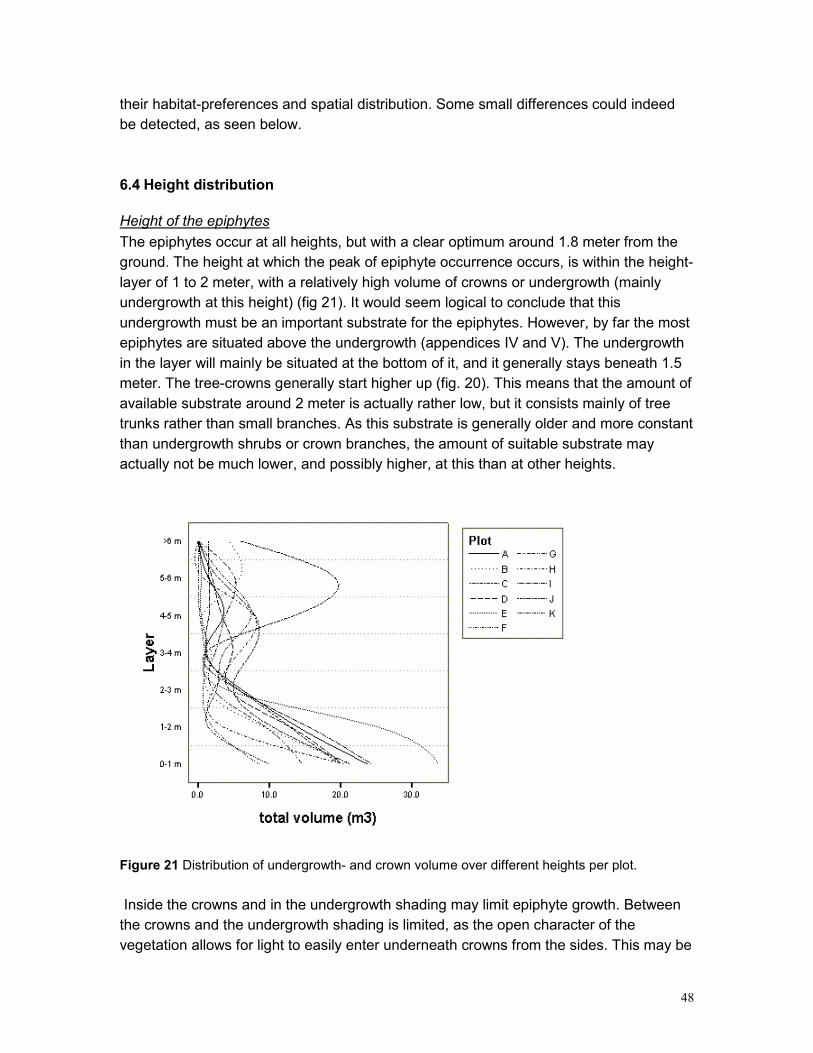
48
their habitat-preferences and spatial distribution. Some small differences could indeed
be detected, as seen below.
6.4 Height distribution
Height of the epiphytes
The epiphytes occur at all heights, but with a clear optimum around 1.8 meter from the
ground. The height at which the peak of epiphyte occurrence occurs, is within the height-
layer of 1 to 2 meter, with a relatively high volume of crowns or undergrowth (mainly
undergrowth at this height) (fig 21). It would seem logical to conclude that this
undergrowth must be an important substrate for the epiphytes. However, by far the most
epiphytes are situated above the undergrowth (appendices IV and V). The undergrowth
in the layer will mainly be situated at the bottom of it, and it generally stays beneath 1.5
meter. The tree-crowns generally start higher up (fig. 20). This means that the amount of
available substrate around 2 meter is actually rather low, but it consists mainly of tree
trunks rather than small branches. As this substrate is generally older and more constant
than undergrowth shrubs or crown branches, the amount of suitable substrate may
actually not be much lower, and possibly higher, at this than at other heights.
Figure 21 Distribution of undergrowth- and crown volume over different heights per plot.
Inside the crowns and in the undergrowth shading may limit epiphyte growth. Between
the crowns and the undergrowth shading is limited, as the open character of the
vegetation allows for light to easily enter underneath crowns from the sides. This may be
49
an important explanation for the abundance of epiphytes at this height. A different factor
that may influence the distribution is the supply of propagules. The chance of a wind-
dispersed seed being intercepted by the crowns and undergrowth is probably higher
than the chance of it landing on a tree trunk, but the first substrate a seed meets in a
crown or shrub is likely to be a leaf or small branch, which can at most allow for
germination, but not for growth to maturity. The relatively open space between 2 and 3 m
may also allow for more air movement carrying wind-dispersed seeds.
The recordings of the climate do not indicate any special characteristic around 2 meter; it
is an intermediate position. If climatic measurements had been taken at more different
heights, e.g. every meter, this might have shown some special feature around 2 meter
that can now not be distinguished.
Height differences between the three families are significant, though not very big.
Especially when looking at the shape of the distributions (appendix III), the difference
does not seem very important. Still, as the order of Orchidaceae growing lower than
Bromeliaceae is a result shared by other studies of upper montane cloud forests (e.g.
Bøgh 1992, Serna 1994), it may reflect a general trend. The lower positions for orchids
could be explained, by their preference for mossy patches (fig.19), which provide their
roots with a moist and rich environment, and which occur most at lower heights. The
reverse is true for the Loranthaceae, which tend to grow on clean branches and need a
young surface to establish themselves, because the haustorium cannot enter old bark
(Goebel 1889). Another possible factor is the difference in seed dispersal between the
families. The distribution of the Loranthaceae is naturally influenced by the behavior of
the birds that disperse them (Godschalk 1983). The plot where most Loranthaceae were
found (plot C) was among the densest and highest plots. High trees may be the
preferred habitat for birds, which may put the Loranthaceae at relatively high positions
compared to the wind dispersed species. Also the birds can not perch on the vertical
trunk, restricting the seed-attachment to relatively small branches, which are most
abundant in the undergrowth and the canopy. Of these two habitats the canopy may be
preferred by the birds, for safety, and may also be more suitable for the mistletoes, for
higher light-intensities and lifespan of the branches.
Ecological equivalence and coexistence
Differences between species, especially the different bromeliads, may be statistically
significant, but most differences are too small to be ecologically significant. Differences
in morphology, like the atmospheric characteristics of Tillandsia sp.1 versus the tank-
habitus of the other abundant species, Racinaea tetrantha and Tillandsia compacta,
could reflect adaptations to a different environment. This could be expected to result in a
different height distribution, but this was not found in this case. However, if the spatial
distribution is most strongly influenced by seed-dispersal, this result is no longer

50
surprising. As the bromeliad species have very similar plumed seeds they would be
expected to be dispersed similarly.
In other studies different Bromeliaceae are usually found to grow at different heights
(Pittendrigh 1948, Bennett 1987, Fischer & Araujo 1995). These studies, however, have
considered a wider range of bromeliad types and a longer climatological gradient in the
forest. In the forest area studied here the circumstances may not be diverse or extreme
enough to cause a differentiation of heights in these bromeliads.
A different explanation could be that the species are in fact ecologically interchangable,
a conclusion that has been drawn for some other groups of epiphytes (Yeaton &
Gladstone 1982, Benzing 1981b). Co-existence is usually considered possible only if
some sort of resource partitioning takes place (De Kroon 1998), which is typically not the
case if species are each others’ ecological equivalents. However, alternative models of
species diversity can describe a situation of cohabitation that is not governed by direct
interactions between plants.
Benzing (1981b) compared the distribution of epiphytes in a dry open forest to that of
sessile organisms on coral reefs and rocky shores. Here patches that become available
for settlement are colonized by the first propagule to arrive, regardless of its competitive
capacity. This chance-mechanism is said to maintain species-diversity in these systems.
The patchiness and variability of the substrate available to epiphytes and the lottery-
aspect of seed arrival at a given site, does indeed to justify such a comparison. Indeed a
similar mechanism has been proposed for cryptogamic epiphytic vegetations, where the
success of a species at a site is determined chiefly by the chance and the time of the
arrival of propagules (Barkman 1958, Wolf 1993).
Only if the suitability of a site changes is the timing to arrive at that site of importance for
the chance of successful establishment. In the situations described above the suitability
is decreased by the settlement of competitors. However, for vascular epiphytes the
situation is a bit different, because competition between species is not an important
mechanism (De Granville 1978). Suitability of a site can still change, e.g. by changing
bark characteristics or light climate, but it is less likely. This means that the spatial
aspect of propagule supply is more important than the timing. Since the substrate can
never be saturated with seeds from one population, there are always suitable sites left
for other species to settle, as long as new sites become available frequently enough
(Benzing 1981b, Bennett 1986), or, as in this forest, as long as many suitable sites have
not yet been occupied. The population sizes of cohabiting species may then simply be a
function of the amount of seeds that have been produced and dispersed in the area
(Yeaton & Gladstone 1982). The differences in abundance of the bromeliad species can
than be explained quite easily, the different population structures indicating a difference
in life-strategies, causing a different seed production, causing a different abundance.

51
Defining the vertical position
Height above the ground is nearly always found to be an important factor for epiphyte
occurrence (e.g. Pittendrigh 1948, Wolf 1993, Hietz 1995), but the circumstances that
determine the occurrence of epiphytes high in the crown may also prevail elsewhere in
the forest. High light intensities at forest edges, e.g. at ridges, clearings or streams, can
allow the canopy epiphytes down to ground level, given the right substrate is found there
(De Granville 1978). The zonations (Johansson 1974) that are so widely used also
indicate that the distribution of epiphytes should be more related to the surrounding
vegetation structure than to height from the ground (fig. 4).
However, the fact that height from the ground is more constant between plots than the
distances of epiphytes to the crown and the undergrowth (appendix IV), is an indication
that in this case height is probably the best measure for describing vertical epiphyte
positions. If a zonation-type measure had been more adequate, the distance from the
top and/or the bottom of the crown should have been more constant, looking at the
variation in a species’ distribution as well as at differences between plots, than the height
from the ground.
Due to the simplicity of the GIS model used, the alternative measures were only vertical
distances, which do not fully consider the structure of the vegetation surrounding the
epiphyte. However, even these simple measures do give an additional dimension to the
information on epiphyte position. Their variability indicates that they are more dependent
on plot-structure than height from the ground is, which means that although the ‘host-
vegetation’ differs considerably in height between plots, the epiphytes stay more or less
at the same height from the ground.
It must be noted here that the situation might be different for communities of cryptogamic
epiphytes. The predominance of lichens, Usnia spp. in particular, and the absence of
green mosses on small branches, usually situated in the periphery of crowns, was
apparent in the field, though no numerical data is available to verify this impression. A
rough idea of the height distribution of different cryptogam-groups can be gotten from
appendix VIII.
6.5 Spatial pattern
Clustering of the epiphytes
The fact that epiphytes had a clustered distribution does not come as a surprise. The
different clustering at different scales indicates, however, that the clustering of the
substrate occurs at several levels. On the xy-projection the epiphytes are clustered most
strongly at small distances. This can be explained by the occurrence of many individuals
straight above each other on vertical tree trunks and close to each other within a tree
crown. Especially the positioning of epiphytes at the same xy-coordinates gives a strong
clustering. At bigger distances, maximum 2.5 meter in these plots, the denseness of
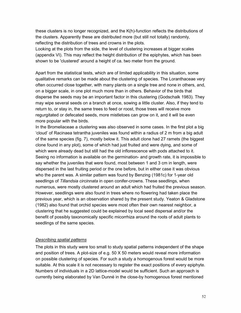
52
these clusters is no longer recognized, and the K(h)-function reflects the distributions of
the clusters. Apparently these are distributed more (but still not totally) randomly,
reflecting the distribution of trees and crowns in the plots.
Looking at the plots from the side, the level of clustering increases at bigger scales
(appendix VI). This may reflect the height distribution of the epiphytes, which has been
shown to be 'clustered' around a height of ca. two meter from the ground.
Apart from the statistical tests, which are of limited applicability in this situation, some
qualitative remarks can be made about the clustering of species. The Loranthaceae very
often occurred close together, with many plants on a single tree and none in others, and,
on a bigger scale, in one plot much more than in others. Behavior of the birds that
disperse the seeds may be an important factor in this clustering (Godschalk 1983). They
may wipe several seeds on a branch at once, sowing a little cluster. Also, if they tend to
return to, or stay in, the same trees to feed or roost, those trees will receive more
regurgitated or defecated seeds, more mistletoes can grow on it, and it will be even
more popular with the birds.
In the Bromeliaceae a clustering was also observed in some cases. In the first plot a big
‘cloud’ of Racinaea tetrantha juveniles was found within a radius of 2 m from a big adult
of the same species (fig. 7), mostly below it. This adult clone had 27 ramets (the biggest
clone found in any plot), some of which had just fruited and were dying, and some of
which were already dead but still had the old inflorescence with pods attached to it.
Seeing no information is available on the germination- and growth rate, it is impossible to
say whether the juveniles that were found, most between 1 and 3 cm in length, were
dispersed in the last fruiting period or the one before, but in either case it was obvious
who the parent was. A similar pattern was found by Benzing (1981c) for 1-year old
seedlings of Tillandsia circinnata in open conifer-crowns. These seedlings, when
numerous, were mostly clustered around an adult which had fruited the previous season.
However, seedlings were also found in trees where no flowering had taken place the
previous year, which is an observation shared by the present study. Yeaton & Gladstone
(1982) also found that orchid species were most often their own nearest neighbor, a
clustering that he suggested could be explained by local seed dispersal and/or the
benefit of possibly taxonomically specific micorrhiza around the roots of adult plants to
seedlings of the same species.
Describing spatial patterns
The plots in this study were too small to study spatial patterns independent of the shape
and position of trees. A plot-size of e.g. 50 X 50 meters would reveal more information
on possible clustering of species. For such a study a homogenous forest would be more
suitable. At this scale it is not necessary to register the exact positions of every epiphyte.
Numbers of individuals in a 2D lattice-model would be sufficient. Such an approach is
currently being elaborated by Van Dunné in the close-by homogenous forest mentioned

53
before. Madison (1979) has also sampled epiphyte distribution on such a scale,
recording the presence of epiphyte species on rubber trees in a 1 ha. plot in a
homogenous plantation. He used a Χ2-test on groups of 5 trees in a row to study
clustering of species. A geo-statistical analysis of the data would probably reveal more
information on the actual spatial distribution, and would be an interesting exercise.
When studying epiphyte clustering at a smaller scale, within one or a few trees, the
distribution of the substrate becomes an important factor, one that is difficult to describe
or quantify. A GIS may prove a useful tool if attempts to do so are to be undertaken (see
chapter 6.10). An alternative method for analyzing spatial patterns of epiphytes, on a
very detailed scale, was described by Hazen (1966), who considered the spatial
distribution as distances along a branch. He transforms the branch to a straight line by
inserting the length of side branches at the points where they branch of, and then
analyses the randomness of epiphyte distribution by their position on this line. However,
his assumption ‘that interaction occurs along a branch, not between neighboring
branches…’ does not seem to justify this one dimensional approach. Vester & Gardette
(1996) proposed ‘three dimensional mapping’, mapping ‘large individuals … individually
and patches of small individuals or colonies … by indicating form, extension and position
of the patch.’ Unfortunately this method is not described to any detail, leaving unclear
whether a truly three dimensional method for mapping has been developed, or whether
two dimensional maps of the tree-shape, as have been used by Dickinson (1993), are
meant, and in what way these maps are to be analyzed. Drawing epiphytes in trees and
forests by side views is a method used by some early researchers (Pittendrigh 1948,
Veloso & Klein 1957, in Smith & Downs 1974), and can provide a fair bit of insight in
epiphyte-patterns. However, a good sideview is difficult to obtain in many forests and the
method is two dimensional, with all the restrictions of such a reduction, and rather
qualitative.
For the moment it seems safe to conclude that a good method for analyzing spatial
distributions of epiphytes has not yet been developed, and the challenge remains to find
a solution to this problem.
6.6 Phorophytes
Loranthaceae, being hemi-parasites, have a very close connection with their hosts. This
could explain the fact that the distribution of this group over the different tree species
differs from that of the Bromeliaceae and Orchidaceae. The absence of Loranthaceae on
Clethra sp. may be caused by some incompatibility-mechanism. Several such
mechanisms have been described (see chapter 1.6), but it will require additional
research to determine what ecological or physiological mechanisms cause the absence
of mistletoes on this Clethra- species. Absence of live Loranthaceae on dead trees can
easily be explained by the lack of sap stream in dead trees, which leaves the mistletoes
without the necessary supply of water and nutrients.

54
The other epiphyte-families do not seem to have a specific preference for host-species,
nor do the different species. Adults and juveniles of a species could theoretically have
different distributions, due to ages of trees or possible incompatibility between epiphyte
and phorophyte having its effects only after some time has passed. Adults and juveniles
of Racinaea tetrantha do show a different distribution over the host-species. However,
the majority (89) of the R. tetrantha juveniles on Clethra were found in only one tree,
which strongly affects this result. It does not seem likely that adults and juveniles have a
significantly different distribution over phorophyte species in this case.
Host specificity, the restriction of an epiphyte species to one or more host-species, has
been reported by some authors (e.g. Went 1940), but has been rejected by others (e.g.
Johansson 1974), and apparently no mechanisms have been demonstrated (Benzing
1995). Variation in the suitability of trees as hosts for epiphytes, including non-vascular
epiphytes, is usually attributed to bark characteristics like roughness (Goebel 1889,
Catling & Lefkovitch 1989, Kernan & Fowler 1995) and chemical composition with regard
to nutrient supply (Gustafsson & Eriksson 1995, Gauslaa et al. 1998) or inhibitory
substances (Frei & Dodson 1972), and sometimes tree age or tree growth rate (Went
1940, Wolf 1993, 1994) and tree-architecture (Migenis & Ackerman 1993).
The main tree-species in this study all had rather similar bark characteristics, with
medium rough trunk-surfaces and smoother branches. The only species with peeling
bark, which has a negative impact on epiphyte establishment (Johansson 1974), were
Tibouchina grossa and Escallonia myrtillioides. These were shrubs and hardly ever high
enough to be recorded as trees, so they would not be expected to harbor many
epiphytes. However, other shrub-species contained quite a few epiphytes, especially
bromeliad juveniles, while these shrubs contained no and very little epiphytes
respectively. This could be attributed to the character of their bark, but also to their
limited age (Tibouchina grossa is typical pioneer-shrub, so will have a high growth rate,
Escallonia propagates quickly by sending out underground runners from which new
shoots rise). A bigger Escallonia tree (DBH ca. 10 cm) outside the plots did contain
considerable numbers of epiphytes, mainly orchids. In contrast to the tendency on other
trees, most epiphytes on this tree were situated in the forks of branches. Those trying to
establish on the trunk had apparently had problems with the peeling bark.
6.7 Plots
Although no significant correlations were found, there does seem to be a positive
relation between the basal area and the number of epiphytes in a plot (p < 0.001 before
Bonferroni correction). This conclusion is justified by the total logic of the relation, more
basal area meaning more substrate for the epiphytes. The weakness of the relation
however, and the lack of correlation of epiphyte numbers with crown-cover or -volume,
even before Bonferroni, may reflect an equilibrium between positive and negative
properties of dense crown-cover for epiphytes: extra availability of substrate vs. extra
shading.
55
Distance to remnants on this scale, where the greatest distance between a plot and a
remnant tree was 68 m, is probably of little importance for supply of propagules,
because of the effective seed dispersal. All species found in this study belonged to
families whose seeds can travel through the air, either in the guts of birds
(Loranthaceae) or being carried by the wind, thanks to minute size (Orchidaceae) or
plumed appendages (Bromeliaceae). Seeds of Guzmania monostachia and Tillandsia
fasciculata (both species in the subfamily Tillandsioideae) remained air-borne for 15 and
12 seconds respectively when dropped from a height of 2 m, compared to 3 seconds for
dandelion seeds (Taraxacum officinalis) (Smith & Downs 1974). From 10 m higher up
the flight time could than be up to 90 seconds, which would allow for dispersal over
considerable distances when there is any wind. It is also likely that frugivorous birds can
disperse the seeds of the Loranthaceae over considerable distances (Hawksworth
1983). This implies that the tall remnants growing inside the studied forest are not
necessarily the only source of epiphyte seeds for this area, but that seeds may also
arrive from the surrounding forests. This idea is supported by the results of Denslow &
Gomez (1990), who found that only a small fraction of the seed rain in forest gaps could
be attributed to adult trees within 50 m, and Martinez-Ramez & Soto-Castro (1993, in
Loiselle et al.), who found that only ca. 50 % of the seed rain in a Mexican wet forest
came from within their 25 x25-m plots.
6.8 Growing sites
Seedlings and small juveniles of Racinaea tetrantha were found growing on leaves of
Clethra sp., on small dead branches and even on ‘branches’ of the fruticose lichen Usnia
sp. and the livermoss Frullania sp. These are obviously not very persistent growing sites,
so these individuals will never grow to maturity. Seedlings and small juveniles of the
same species and Tillandsia sp.1 were also encountered on young W. pubescens-trees.
The substrate in these cases was a shorthaired green skin rather than corky tree bark.
These examples indicate that germination can occur on many different substrates.
Unfortunately, since young Weinmannia-shoots don’t remain the way they are either, the
fate of epiphytes on such substrates can not be studied independently of the unstable
character of their substrate.
In this study no preference for compass orientation was found. Bennett (1987) did find
an aspect preference for a bromeliad species in Florida, but not for others. If this finding
reflects any ecological differentiation, based on a light or moisture difference, this is
expected to be stronger in Florida than in Colombia, on account of the latitude. Also it
would be expected to be more pronounced in trees with a bigger diameter.
Branch inclination does not seem to limit epiphyte settlement in this forest. The high
proportion of epiphytes growing on vertical branches probably reflects the high
proportion on tree trunks. This can also be seen in the height-distribution of the
epiphytes.
56
There are no indications that 'canopy soil', humus accumulation on branches, has an
influence on the epiphytes in this study. Very few epiphytes were found growing on forks
of branches, a result shared by the study of bromeliads by Hanke (1999). Freiberg
(1996) finds the biggest diversity of vascular epiphytes in a tropical lowland rain forest
tree on the topside of branches, and attributes this to the humus layer present there.
Rudolph et al. (1998) defined the surface available for settlement by vascular epiphytes
in a tropical lowland rain forest as the upper half of the branches, and ignored ‘the few’
epiphytes growing on the underside. In the present study, however, the top was the least
frequented side of the branches, while the sides were frequented most. This may be
explained quite simply by the characteristics of the trees, which are relatively small and
young and with little humus accumulation on the branches. The ‘preference’ for the sides
also reflects the preference for vertical stems, which only have sides.
However, Bøgh (1992), studying epiphytes in an undisturbed montane rain forest at
2,900 m in Ecuador, also found relatively little epiphytes growing in humus deposits. A
possible explanation for the difference in humus dependence of epiphytes between
tropical montane rain forests and lowland rain forests, may be the different importance of
the water storing characteristics of humus and its role in maintaining a moist
microclimate (Freiberg 1997). These properties are probably more important in hot
lowland forests, where recurrent drought is a common canopy-feature, than in the much
cooler and wetter montane forests (Bøgh 1992).
The character of the epiphytes could also be another explanation for the lack of
preference for humous sites. Most epiphytes were hemi-parasites (Loranthaceae) or
tank and/or atmospheric epiphytes (Bromeliaceae). These are not dependent on humus
for water or nutrients, so they do not need to follow patterns of humus accumulation,
even if there is any. The only species that may be humus-dependent, are some
Orchidaceae. A species that is certainly a humus-epiphyte is Orchidaceae sp.1, which
was found on stem-bases only. The most abundant orchid, Orchidaceae sp.5, did have
roots partly growing underneath mats of mosses, where a thin humus layer may have
developed, but roots also grew on exposed bare bark, and orchid roots can take up
water and nutrients directly from rain and mist (see chapter 1.5). The many species of
rarer orchids varied in their apparent humus- preference.
6.9 Plant appearance
Close to the ground the environment is darker and more moist, and bromeliads that grow
here are greener than those growing at more exposed sites higher up in the plot. For
Tillandsia compacta this correlation is not very strong. This may be due to the lower
number of plants tested, but it could also reflect a lower plasticity in this species
compared to Racinaea tetrantha.
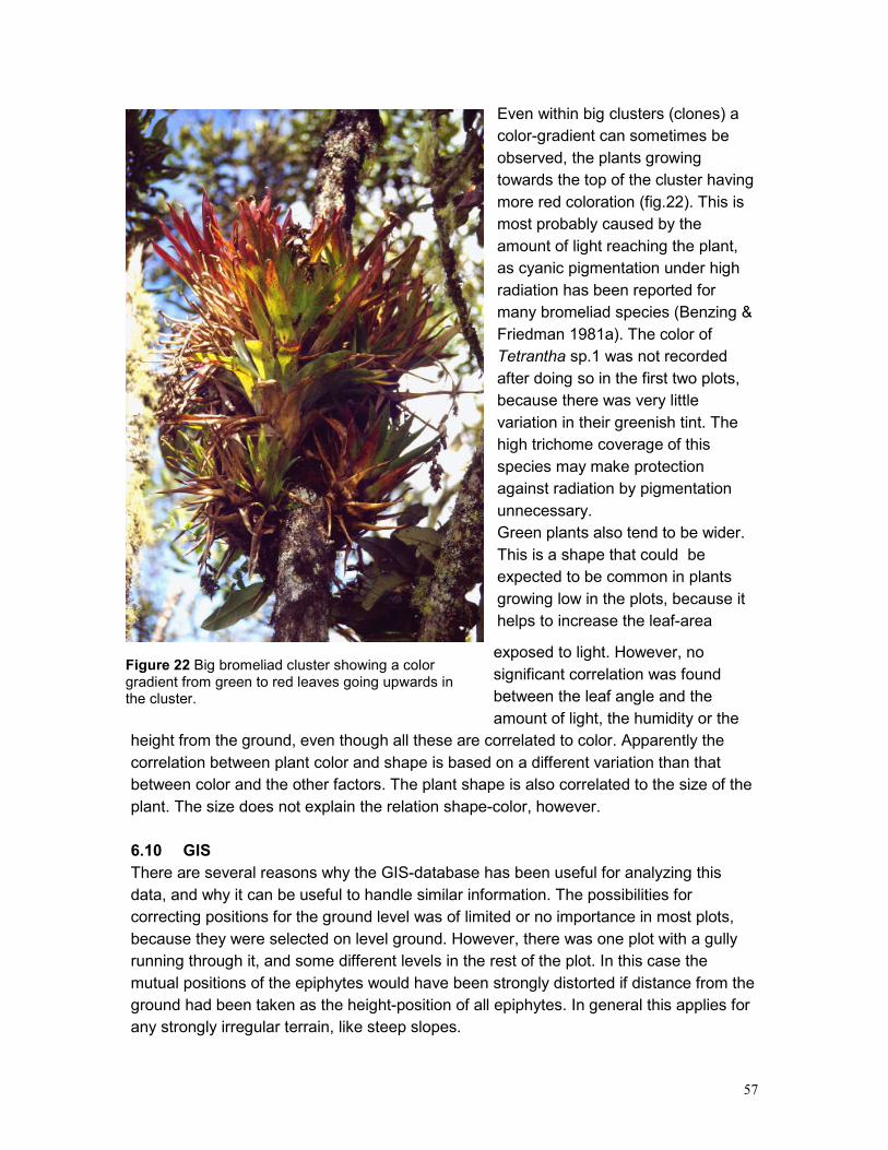
57
Even within big clusters (clones) a
color-gradient can sometimes be
observed, the plants growing
towards the top of the cluster having
more red coloration (fig.22). This is
most probably caused by the
amount of light reaching the plant,
as cyanic pigmentation under high
radiation has been reported for
many bromeliad species (Benzing &
Friedman 1981a). The color of
Tetrantha sp.1 was not recorded
after doing so in the first two plots,
because there was very little
variation in their greenish tint. The
high trichome coverage of this
species may make protection
against radiation by pigmentation
unnecessary.
Green plants also tend to be wider.
This is a shape that could be
expected to be common in plants
growing low in the plots, because it
helps to increase the leaf-area
exposed to light. However, no
significant correlation was found
between the leaf angle and the
amount of light, the humidity or the
height from the ground, even though all these are correlated to color. Apparently the
correlation between plant color and shape is based on a different variation than that
between color and the other factors. The plant shape is also correlated to the size of the
plant. The size does not explain the relation shape-color, however.
6.10 GIS
There are several reasons why the GIS-database has been useful for analyzing this
data, and why it can be useful to handle similar information. The possibilities for
correcting positions for the ground level was of limited or no importance in most plots,
because they were selected on level ground. However, there was one plot with a gully
running through it, and some different levels in the rest of the plot. In this case the
mutual positions of the epiphytes would have been strongly distorted if distance from the
ground had been taken as the height-position of all epiphytes. In general this applies for
any strongly irregular terrain, like steep slopes.
Figure 22 Big bromeliad cluster showing a color gradient from green to red leaves going upwards in the cluster.

58
The most important reason to use a GIS however, is the possibility to analyze data
topologically, e.g. linking the position of epiphytes to the vegetation structure (crowns
and undergrowth). As yet the possibilities for exploiting the 3-dimensionality of the
information are rather limited, but three-dimensional GIS-systems will probably become
available in the future (Raper & Kelk 1991, Hack & Sides 1994, Breunig 1999). Apart
from the simple vertical distances as calculated within this research, it may than be
possible for example, to deduct the amount of shading at a given position by counting
the crown-surfaces within a cone or hemisphere above it.
In many epiphyte studies the trees are sampled per zone (Johansson 1974), which may
obscure alternative patterns of epiphyte occurrence. Dickinson et al. (1993), who
mapped all epiphyte communities on an emergent tree (drawing the tree with the
communities on it), could confirm the zonations in epiphyte communities only for the
outer canopy, while the inner canopy showed complex patterns. Registering epiphyte-
positions independently of any presumed zones or categories, purely spatially, may be a
method to overcome the limitations of zonation-systems, especially with the
development of methods to link various ecological parameters to the sites in GIS. By
storing the exact position of the epiphytes and the phorophytes, the position of epiphytes
in any of the zones-systems as used by Johansson (1974) and many others, can still be
deduced from the data, even if it was not registered in the field. In this way comparisons
can easier be made with data of previous studies. To be able to do this with more detail,
some additional parameters will have to be measured in the field, to create a more
realistic model of tree-architecture than a wide cylinder (crown) on a narrow cylinder
(stem). Such a model could also be very useful for estimating substrate (branch surface)
quantities. Co-operation with tree-architecture specialists would be advisable.
Another application for GIS in canopy research could be 3D-network analysis, e.g. to
calculate the efficiency of ant-routes between their nest and different food-sources, or
dispersal of bromeliad tank inhabitants. The positions of nests, food or bromeliads could
be combined with the pattern and characteristics of branches connecting the sites. The
animal characteristics could be an additional aspect of such a database: flying or
jumping animals would have quite different routes than those confined to walking, and
the branches will look quite different to big or small animals and to predators and preys,
to name a few examples. The possibility for integration of such different kinds of spatial
and thematic data makes GIS especially suitable for some ecological applications, also
in three dimensions.
A third advantage of having the data in a GIS, are the graphic possibilities for
representing the data, as maps. Appendix II shows some possibilities readily available. It
is as yet not possible to represent stacks of points or floating cylinders ('tree crowns') in
a 3D picture within GIS software. Three-dimensional drawing programs, usually used for
designing purposes, can make such representations, but lack a ready possibility for
entering the data as co-ordinates in a table or from a GIS coverage or grid, as would be
necessary in this case. Integration of 3D graphics software and GIS sytems are being

59
worked on, however, so these problems will be probably be solvable in the future
(Hoinkes & Lange 1995, Verbree et al. 1999).
7 Conclusion
The development of methods for describing (spatial) epiphyte distribution remains a
challenge. The possibilities of GIS as a tool in such methods need more investigation,
and will increase strongly when 3-dimensional GIS will become available.
Some patterns in the distribution of epiphytes have been detected in this explorative
study. However, to get insight into the mechanisms underlying these patterns, a more
detailed, preferably experimental research would be necessary.
The different population structures of the bromeliad species form another subject calling
for a closer investigation. Different life-strategies could be at the base of this, and these
could be important in influencing the rate and patterns of dispersal of different epiphyte-
species.
60
References
Ackerman J.D. 1986. Coping with the epiphytic existence: pollination strategies.
Selbyana 9: 52-60.
Adams III W.W. & C.E. Martin 1986a. Physiological consequences of changes in life
form of the Mexican epiphyte Tillandsia deppeana (Bromeliaceae). Oecologia 70: 298-
304.
Adams III W.W. & C.E. Martin 1986b. Heterophylly and its relevance to evolution within
the Tillandsioideae. Selbyana 9: 121-125.
Awasthi O.P., E. Sharma & L.M.S. Palni 1995. Stemflow: a source of nutrients in some
naturally growing epiphytic orchids of the Sikkim Himalaya. Annals of Botany 75: 5-11.
Bader M., H.J.F. van Dunné & H.J. Stuiver In prep. The application of a geographical
information system (GIS) in an epiphyte study.
Barkman J.J. 1958. Phytosociology and ecology of cryptogamic epiphytes. Van Gorcum
& Comp. N.V., Assen.
Barlow B.A. 1983. Biogeography of Loranthaceae and Viscaceae. In: Calder D.M. & P.
Bernhardt 1983. The biology of mistletoes. Academic Press, Sydney.
Bennett B.C. 1986. Patchiness, diversity, and abundance relationships of vascular
epiphytes. Selbyana 9: 70-75.
Bennett B.C. 1987. Spatial distribution of Catopsis and Guzmania (Bromeliaceae) in
southern Florida. Bulletin of the Torrey Botanical Club 114(3): 265-271.
Benzing D.H. 1981a. Why is Orchidaceae so large, it’s seeds so small, and it’s
seedlings mycotrophic? Selbyana 5(3-4): 241-242.
Benzing D.H. 1981b. Bark surface and the origin and maintenance of diversity among
angiosperm epiphytes: a hypothesis. Selbyana 5(3-4): 248-255.
Benzing D.H. 1981c. The population dynamics of Tillandsia circinnata (Bromeliaceae):
Cypress crown colonies in southern Florida. Selbyana 5(3-4): 256-263.
Benzing D.H. & W.E. Friedman 1981a. Patterns of foliar pigmentation in Bromeliaceae
and their adaptive significance. Selbyana 5(3-4): 224-240.
Benzing D.H. & W.E.Friedman 1981b. Mycotrophy: its occurrence and possible
significance among epiphytic Orchidaceae. Selbyana 5(3-4): 243-247.
Benzing D.H. 1986. The vegetative basis ofvascular epiphytism. Selbyana 9: 23-43.

61
Benzing D.H. 1989a The evolution of epiphytism. Pp.15-41. In: Lüttge, U. (ed.),
Vascular plants as epiphytes, Evolution and Ecophysiology. Ecological Studies 76,
Springer-Verlag, Berlin-New York.
Benzing D.H. 1989b The mineral nutrition of epiphytes. Pp.167-199. In: Lüttge, U. (ed.),
Vascular plants as epiphytes, Evolution and Ecophysiology. Ecological Studies 76,
Springer-Verlag, Berlin, New York.
Benzing D.H. 1990. Vascular epiphytes. Cambridge University Press, Cambridge. 354
pp.
Benzing D.H. 1995. Vascular epiphytes. Pp.225-254. In: Lowman, M.D. & N.M.
Nadkarni (eds.), Forest Canopies. Academic Press, Inc.
Bøgh A. 1992. Composition and distribution of the vascular epiphyte flora of an
Equadorianmontane rain forest. Selbyana 13: 25-34.
Bouchon J., Ph. de Reffye & D. Barthelemy 1997. Modelisation et simulation de
l’architecture des vegetaux. INRA, Paris.
Breunig M. 1999. An approach to the integration of spatial data and systems for a 3D
geo-information system. Computers & Geosciences 25: 39-48.
Calder D.M. 1983. Mistletoes in focus: an introduction. In: Calder D.M. & P. Bernhardt
1983. The biology of mistletoes. Academic Press, Sydney.
Cavalier J. 1995. Reforestation with the native tree Alnus acuminata: effects on
phytodiversity and species richness in an upper montane rain forest area of Colombia.
In: Hamilton L.S., J.O. Juvik & F.N. Scatena 1995. Tropical montane cloud forests.
Springer Verlag, New York.
Cavalier J & G. Goldstein 1989. Mist and fog interception in elfin cloud forests in
Colombia and Venezuela. Journal of Tropical Ecology 5: 309-322.
Cavalier J., D. Solis & M.A. Jaramillo 1996. Fog interception in montane forests across
the Central Cordillera of Panamá. Journal of Tropical Ecology 12: 357-369.
Cressie N. A. C. 1993. Statistics for spatial data. Revised edition. John Wiley & Sons,
Inc., New York.
Davidson D.W. 1988. Ecological studies of neotropical ant gardens. Ecology 69(4):
1138-1152.
Davidson D.W. & W.W. Epstein 1989. Epiphytic associations with ants. . In: Lüttge, U.
(ed.), Vascular plants as epiphytes, Evolution and Ecophysiology. Ecological Studies 76,
Springer-Verlag, Berlin-New York.
62
De Kroon J.C.J.M. 1998. College plantenecologie. Collegedictaat Leerstoelgroep
Natuurbeheer en Plantenecologie, LUW, Wageningen.
Denslow J.S. & A.E. Gomez Diaz 1990. Seed rain to tree-fall gaps in a Neotropical rain
forest. Canadian Journal of Forestry Research 20: 642-648.
Dickinson K.J.M., A.F. Mark & B. Dawkins 1993. Ecology of lianoid/epiphytic
communities in coastal podocarp rain forest, Haast Ecological District, New Zealand.
Journal of Biogeography 20: 687-705.
Finnegan 1996. Patterns & processes in neotropical secondary rain forest: the first 100
years. Trends in Ecology & Evolution 11(3): 119-123.
Fischer E.A. & A.C. Araujo 1995. Spatial organization of a bromeliad community in the
Atlantic rainforest, southeastern Brazil. Journal of Tropical Ecology 11: 559-567.
Frei J.K. & C.H. Dodson 1972. The chemical effect of certain bark surfaces on the
germination and early growth of epiphytic orchids. Bulletin of the Torrey Botanical Club
99: 301-307.
Freiberg M. 1996a. Spatial distribution of vascular epiphytes on three emergent canopy
trees in French Guiana. Biotropica 28(3): 345-355.
Freiberg M. 1996b. phenotype expression of epiphytic Gesneriaceae under different
microclimatic conditions in Costa Rica. Ecotropica 2: 49-57.
Freiberg M. 1997. Spatial and temporal pattern of temperature and humidity of a tropical
premontane rain forest tree in Costa Rica. Selbyana 18(1): 77-84
Gauslaa Y., M. Ohlson & J. Rolstad 1998. Fine-scale distribution of the epiphytic lichen
Usnea longissima on two even aged neighbouring Picea abies trees. Journal of
vegetation Science 9: 95-102.
Godschalk S.K.B. 1983. Mistletoe dispersal by birds in South Afrika. In: Calder M. & P.
Bernhardt 1983. The biology of mistletoes. Academic Press, Sydney.
Goebel K. 1889. Pflanzenbiologische Schilderungen. Ch.3: Epiphyten. N.G.Elwert’sche
Verlagsbuchhandlung, Marburg.
Goh C.J. & M. Kluge 1989. Gas exchange and water relations in epiphytic orchids.
Pp.139-166. In: Lüttge, U. (ed.), Vascular plants as epiphytes, Evolution and
Ecophysiology. Ecological Studies 76, Springer-Verlag, Berlin, New York.
Guevara S., J. Laborde & G. Sánchez 1998. Are isolated remnant trees in pastures a
fragmented canopy? Selbyana 19(1): 34-43.
Hack R. & E. Sides 1994. Three-dimensional GIS: recent developments. Seminar
report, ITC Journal 1994(1): 64-72.

63
Hamilton L.S., J.O. Juvik & F.N. Scatena 1995. Tropical montane cloud forests.
Springer Verlag, New York.
Hanke J.K. 1999. An explorative study of patterns in the distribution of epiphytic
bromeliads in a secondary upper montane forest, Colombia. Internal report no. 323,
Hugo de Vries Laboratory, University of Amsterdam.
Hartshorn G.S. 1980. Neotropical forest dynamics. In:Tropical succession.
Hawksworth F.G. 1983. Mistletoes as forest parasites. In: Calder M. & P. Bernhardt
1983. The biology of mistletoes. Academic Press, Sydney.
Hietz P. & U. Hietz-Seifert 1995a. Composition and ecology of vascular epiphyte
communities along an altitudinal gradient in central Veracruz, Mexico. Journal of
Vegetation Science 6: 487-498.
Hietz P. & U. Hietz-Seifert 1995b. Structure and ecology of epiphytic communities of a
cloud forest in central Veracruz, Mexico. Journal of Vegetation Science 6: 719-728.
Hietz P. 1997. Population dynamics of epiphytes in a Mexican humid montane forest.
Journal of Ecology Oxford 85: 767-775.
Hietz P. & O. Briones 1998. Correlation between water relations and within-canopy
distribution of epiphytic ferns in a Mexican cloud forest. Oecologia 114: 305-316.
Hoinkes R. & E. Lange 1995. Toolkit expands visual dimensions in GIS. GIS World
8(7): 54-56.
Horn H.S. 1971. The adaptive geometry of trees. Princeton University Press, Princeton.
Huxley C. 1980. Symbiosis between ants and epiphytes. Biological Review 55: 321-340.
Johansson D. 1974. Ecology of vascular epiphytes in West African rain forest. Acta
Phytogeogr. Suec. 59. Uppsala.
Kapelle M. 1995. Ecology of mature and recovering Talamancan montane Quercus
forests, Costa Rica. PhD dissertation, University of Amsterdam.
Kenkel N.C. & G.E. Bradfield 1986. Epiphytic vegetation on Acer macrophyllum: a
multivariate study of species-habitat relationships. Vegetatio 68: 43-53.
Kernan C. & N. Fowler 1995. Different substrate use by epiphytes in Corcovado
National Park, Costa Rica: a source of guild structure. Journal of Ecology 83: 65-73.
Kleinfeldt S.E. 1978. Ant-gardens: the interaction of Codonanthe crassifolia
(Gesneraceae) and Crematogaster longispina (Formicidae). Ecology 59(3): 449-456.
Koop H. 1989. Forest dynamics-SILVI-STAR: a comprehensive monitoring system.
Springer Verlag, New York.
64
Kress W.J. 1989. The systematic distribution of vascular epiphytes. Pp.234-261. In:
Lüttge, U. (ed.), Vascular Plants as epiphytes, Evolution and Ecophysiology. Ecological
Studies 76, Springer-Verlag, Berlin-New York.
Lamont B. 1983. Germination of mistletoes. In: Calder D.M. & P. Bernhardt 1983. The
biology of mistletoes. Academic Press, Sydney.
Legendre P. & L. Legendre 1998. Numerical ecology, second english edition.
Development in Environmental Modelling 20, Elsevier, Amsterdam.
Liddy J. 1983. Dispersal of Australian mistletoes: the Cowiebank study. In: Calder D.M.
& P. Bernhardt 1983. The biology of mistletoes. Academic Press, Sydney.
Loiselle B.A., E. Ribbens & O. Vargas 1996. Spatial and temporal variation of seed
rain in a tropical lowland wet forest. Biotropica 28(1): 82-95.
Lowman M.D. & N.M. Nadkarni (eds.) 1995. Forest Canopies. Academic Press, Inc.
Lüttge U. 1997. Physiological Ecology of Tropical Plants. Springer-Verlag, Berlin. 384
pp.
Lüttge U. 1989. Vascular Epiphytes: Setting the Scene. Pp.1-14. In: Lüttge, U. (ed.),
Vascular plants as epiphytes, Evolution and Ecophysiology. Ecological Studies 76,
Springer-Verlag, Berlin-New York.
Madison M. 1977. Vascular epiphytes: their systematic occurrence and salient features.
Selbyana 2(1): 1-13.
Madison M. 1979. Additional observations on ant-gardens in Amazonas. Selbyana 5(2):
107-115.
Martin C.E. 1994. Physiological ecology of the Bromeliaceae. The Botanical Review
60(1): 1-82.
Migenis L.E. & J.D. Ackerman 1993. Orchid-phorophyte relationships in a forest
watershed in Puerto Rico. Journal of Tropical Ecology 9: 231-240.
Moffett M.W. & M.D. Lowman 1995. Canopy access techniques. In: Lowman, M.D. &
N.M. Nadkarni (eds.), Forest Canopies. Academic Press, Inc.
Mora Gil V.I. 1999. Estructura y desarollo de jardines de hormigas en bosques
tropicales secundarios (Araracuara, Caquetá, Colombia). Thesis-report, departamento
de biología, Universidad de Antióquia Medellín.
Nadkarni N.M. 1986. The nutritional effects of epiphytes on host trees with special
reference to alteration of precipitation chemistry. Selbyana 9: 44-51.
Nieder J. & G. Zotz 1998. Methods of analyzing the structure and dynamics of vascular
epiphyte communities. Ecotropica 4: 33-39.

65
Oksanen J. 1988. Impact of habitat, substrate and microsite classes on the epiphytic
vegetation: Interpretation using exploratory and canonical correspondence analysis.
Ann. Bot. Fennici 25: 59-71.
Oostermeijer J.G.B., R. van ‘t Veer & J.C.M. den Nijs 1994. Population structure of
the rare, long-lived perennial Gentiana pneumonanthe in relationto vegetation and
management in the Netherlands. Journal of Applied Ecology 31: 428-438.
Parker G.G. 1995. Structure and microclimate of forest canopies. In: Lowman, M.D. &
N.M. Nadkarni (eds.), Forest Canopies. Academic Press, Inc.
Perry D.R. & J. Williams 1981. The tropical rain forest canopy: a method providing total
access. Biotropica 13(4): 283-285.
Pittendrigh C.S. 1948. The bromeliad-Anopheles-malaria complex in Trinidad. I-the
bromeliad flora. Evolution 2: 58-89.
Raper J.F. & B. Kelk 1991. Three-dimensional GIS. In: Maguire R.J., M.F. Goodchild &
D.W. Rhind (eds.) 1991. Geographical Information Systems. Longman Scientific &
Technical, New York.
Reiners W.A. & R.K. Olson 1984. Effects of canopy components on throughfall
chemistry: An experimental analysis. Oecologia 63: 320-330.
Rudolph D., G. Rauer, J. Nieder & W. Barthlott 1998. Distributional patterns of
epiphytes in the canopy and porophyte characteristics in a western Andean rain forest in
Ecuador. Selbyana 19(1): 27-33.
Sallé G. 1983. Germination and establishment of Viscum album L. In: Calder M. & P.
Bernhardt 1983. The biology of mistletoes. Academic Press, Sydney.
Schimper A.F.W. 1888. Die epiphytische Vegetation Amerikas. Botanische
Mittheilungen aus den Tropen 2, Gustav Fischer, Jena.
Serna Isaza R.A. 1994. Distribución vertical de epífitas vasculares en un relicto de
bosque de Weinmannia tomentosa y Drimys granadensis en la región de Monserrate,
Cundinamarca, Colombia. In: Mora-Osejo L.E. & H. Sturm (eds.) 1994. Estudios
ecologicos del paramo y del bosque altoandino en la Cordillera Oriental de Colombia.
Tomo II. Academia Colombiana de Ciencias exactas, fisicas y naturales, Bogotá.
Smith J.A.C. 1989. Epiphytic Bromeliads. Pp.109-138. In: Lüttge, U. (ed.), Vascular
Plants as epiphytes, Evolution and Ecophysiology. Ecological Studies 76, Springer-
Verlag, Berlin-New York.
Smith L.B. & R.J. Downs 1974. Flora Neotropica, Monograph No. 14, part 1:
Pitcairnioideae (Bromeliaceae). Hafner Press, New York.

66
Smith L.B. & R.J. Downs 1977. Flora Neotropica, Monograph No. 14, part 2:
Tillandsioideae (Bromeliaceae). Hafner Press, New York.
Smith L.B. & R.J. Downs 1979. Flora Neotropica, Monograph No. 14, part 3:
Bromelioideae (Bromeliaceae). Hafner Press, New York.
Sugden A.M. & R.J. Robins 1979. Aspects of the ecology of vascular epiphytes in
Colombian cloud forests, I. The distribution of the epiphytic flora. Biotropica 11(3): 173-
188.
Sugden A.M. 1981.Aspects of the ecology of vascular epiphytes in two Colombian cloud
forests. II. Habitat preferences of Bromeliaceae in the Serrania de Macuira. Selbyana
5(3-4): 264-273.
Ter Steege H. & J.H.C. Cornelissen 1989. Distribution and ecology of vascular
epiphytes in lowland rainforest of Guyana. Biotropica 21(4): 331-339.
Ule E. 1902. Ameisengärten im Amazonasgebiet. Botanische Jahrbücher für
Systematik, Pflanzengeschichte und Pflanzengeographie 30. Beiblatt nr. 68: 45-52.
Van der Hammen T., A. Pérez & P. Pinto (eds.) 1983. La Cordillera Central
Colombiana, Transecto Parque Los Nevados (Introdución y datos iniciales). Stud. Trop.
Andean Ecosyst. 1:1-345. Cramer, Vaduz.
Van der Hammen T., S. Diaz-Piedrahita & V.J. Alvarez (eds.) 1989. La Cordillera
Central Colombiana, Transecto Parque Los Nevados (Segunda Parte). Stud. Trop.
Andean Ecosyst. 3:1-600. Cramer, Berlin-Stuttgart.
Van der Hammen T. & A.G. dos Santos (eds.). La Cordillera Central Colombiana,
Transecto Parque Los Nevados (Cuarta Parte). Stud. Trop. Andean Ecosyst. 4. Cramer,
Berlin-Stuttgart
Veneklaas E.J. 1990a. Nutrient fluxes in bulk precipitation and throughfall in two
montane tropical rain forests, Colombia. Journal of Ecology 78: 974-992.
Veneklaas E.J. 1990b. Rainfall interception and aboveground nutrient fluxes in
Colombian montane tropical rain forest. PhD dissertation, University of Utrecht.
Verbree E., G. van Maren, R. Germs, F. Jansen & M. Kraak 1999. Interaction in virtual
world views – linking 3D GIS with VR. International Journal of Geographical Information
Science 13(4): 385-396.
Vester H.F.M. & E. Gardette 1996. Epiphyte sampling in a three-dimensional
framework. In: Gradstein S.R. et al. 1996. How to sample the epiphytic diversity of
tropical rain forests. Ecotropica 2: 59-72.

67
Went F.W. 1940. Soziologie der Epifyten eines tropischen Urwaldes. Ann. Jard. Bot.
Buitenz., 50: 1-98.
Whitacre D.F. 1981. Additional techniques and safety hints for climbing tall trees, and
some equipment and information sources. Biotropica 13(4): 286-291.
Williams-Linera G., V. Sosa & T. Platas 1995. The fate of epiphytic orchids after
fragmentation of a Mexican cloud forest. Selbyana 16(1): 36-40.
Wolf J.H.D. 1993. Ecology of epiphytes and epiphyte communities in montane
rainforests, Colombia. PhD dissertation, University of Amsterdam.
Wolf J.D.H. 1994. Factors controlling the distribution of vascular and non-vascular
epiphytes in the Northern Andes. Vegetatio 112: 15-28.
Yeaton R.I. & D.E. Gladstone 1982. Thepattern ofcolonization of epiphytes on calabash
trees (Cresentia alata HBK.) in Guanacaste province, CostaRica. Biotropica 14(2): 137-
140.
Young L.Y. & J.H. Young 1998. Statistical Ecology. Kluwer Academic Publishers,
Boston-Dordrecht-London.

68
Appendix I : Evaluation of some methods
Field methods
Apart from the methods described in this report, many others have been considered or
tried out, but have been considered unsuitable or unnecessary. Such 'failures' are
however an integrated part of any research, and can be very interesting for others doing
similar work, encountering similar problems. Also they may answer some 'but why didn't
they…?' questions.
One idea was to catch mist at different heights, to see if there were differences in
amount and nutrient-contents (which could be important to the more atmospheric
Bromeliads). Some ‘fog catchers' were constructed, using plastic mosquito mesh. This
material was shaped into cylinders and cones attached to funnels. A roof-structure kept
out the rain, catching only the ‘horizontal precipitation’. Unfortunately these fog catchers
didn’t work (no water was collected at all), though similar constructions have been used
successfully in other studies (Cavalier & Goldstein 1989, Cavalier et al. 1996). In these
studies the volume of fog intercepted by the mesh was calculated by subtracting the
amount of rain caught in rain gauges from the amount of rain and fog in the fog catchers.
These fog catchers did not have roofs, like the ones tried out in this study did. This might
somehow explain the difference, because mist was certainly a frequent phenomena in
the area.
Another idea was to collect water from Bromeliad-tanks (to measure pH and nutrient
content). This could be done, but only very large plants contained enough water for
analysis, so no systematic sampling was possible. Also the water contained by one plant
was very different in leaf-axis of different ages (the older leaves containing much more
organic material), which might cause a higher variation within the plant than between
plants. Therefor the sampling of tank-water was only carried out to get an indication on
tankwater characteristics in general.
To get an indication of the light-circumstances in the different plots, fish-eye photography
was going to be used. Unfortunately something was wrong with the camera, and after it
was sent away to be repaired it never came back.
Some ideas could be, and were carried out in the field, but turned out to have been a lot
of work for little result. This applies to the description of the Bromeliads, which was done
more elaborately than necessary. This is mainly due to the novelty of the species;
afterwards it was easy to think of better measures. Also it was due to the original plan to
measure more direct environmental variables at the plant itself, to relate those to the
plant's morphology (including plant shape, color, and also leaf-thickness and trichome-
cover).
For example: The color of Bromeliads was at first described with the help of color-charts.
After the experience of 2 plots, seeing less variation in the shades than had been
expected, it was decided to revert to a distinction between red and green, and the
pattern. This was taken for the middle and tip of the leaf separately, which wouldn't have

69
been necessary either, because they were later merged again to get one color-index-
number per plant. At first the color of all Bromeliads was described, later only that of
Racinaea tetrantha and Tillandsia compacta adults within reach of the photometer.
Also the undergrowth was divided into two layers where these were obviously present.
Two DEM’s were made from these layers, which caused problems with intersecting
layers where one of the layers was not present. The DEM of the top layer was made so
that it was never lower than the bottom layer. In the end the DEM of the top layer was
the only one used for the analysis, and it would have been a lot easier to describe this
layer only. If the thickness (vertical size)of the layers had also been recorded, the
constructions of the DEM’s would have been even more complicated, but more extra
information would have been deduced from the division of the 2 layers. However, as
very few epiphytes occurred far under the top of second layer of the undergrowth, this
extra infomation would not have added much ecological information about the epiphytes.
Analysis
The analysis of the data turned out to be rather complicated, because of the unusual
dataset. Several statistical techniques were tried out, but many did not produce any
interesting results, and others were simply not possible.
An hierarchical clustering of 1-m height layers on their species composition was carried
out and the resulting clusters (taking only 4) were compared for several environmental
factors, among which climatic variables. A significant difference between clusters was
found, but the difference did not correspond with the order of division in the clustering
dendrogram.
Although ordinations have been used succesfully for vegetation data of cryptogamic
epiphytes (Kenkel & Bradfield 1986, Oksanen 1988, Wolf 1993), analysis of the ‘height-
zone-plots’ mentioned before, using several ordination methods ((D)CA, CCA, PCA), did
not yield very exiting results (most variation was explained by the ‘variables’ ‘plot A’ and
‘plot C’). An explanation of this may be that ‘species composition’ is not exactly what was
studied in this research, and that variation in the species data was probably too small to
be suitable for correspondence analysis. The epiphytic ‘vegetation’ has a much higher
surface-cover of mosses and lichens than of vascular epiphytes in most places. Taking
only the vascular plants, even only the angiosperms, does not give a representation of a
community, but of individual populations, which apparently have little interaction with
each other.
Another promising option was to cluster the epiphytes spatially and investigate the
species-composition of the clusters, to detect clustering of species. The epiphytes could
indeed be clustered, using the three co-ordinates as the input for a hierarchical cluster
analysis (using euclidean distance as the distance measure, best results with nearest
neighbor for the cluster method). However, investigating the resulting clusters turned out
to be more difficult than expected. The most suitable method would be a Χ2 –test, but
this would require a calculation of all expected values for the species in the clusters,

70
which would be very impractical. Besides that, a lot of the clusters would turn out very
small (groups of 1, 2 or 3 outlying epiphytes), which would make it necessary to group
them to be able to use them in a Χ2 –test, which would disturb the whole idea of the
analysis.
Not all data collected in the field have yet been used in the analysis, nor have all
possible analysis been carried out or has all information been extracted from the data.
However, a fair amount has been, sufficient to distinguish some patterns and attempt
some answers. Most explanations of results remain rather speculative, adding an extra
portion to the speculations of other epiphyte-researchers, which is as far as we might
ever get at truly understanding any ecosystem.

71
Appendix II-1: Maps of the plots: some graphics
DEM of the undergrowth of plot A. The way the shrub layer was sampled, in a regular grid, and the type of interpolation between the measured points, were not ideal for the construction of a realistic model of the undergrowth. This influences the value of figure 21, showing the distribution of undergrowth-volume. Sampling and interpolation methods need adjustment to serve specifically for describing a vegetation surface.
A sketch of a 3D model, as could be made using CAD techniques. Making such a picture representing the data could be done by linking GIS and CAD systems, and in the future by using 3D GIS. Better crown shell models would be desirable, and some existing models may be of use (e.g. Horn 1971, Koop 1989). Another option (depending on the studied scale) could be the use of detailed models of tree architecture (e.g. Bouchon et al. 1997).
Using Virtual Reality graphics may be an interesting possibility in the future (e.g. Verbree et al. 1999).

72
Appendix II-2: Plot A

73
Appendix II-3: Plot B

74
Appendix II-4: Plot C

75
Appendix II-5: Plot D

76
Appendix II-6: Plot E

77
Appendix II-7: Plot F

78
Appendix II-8: Plot G

79
Appendix II-9: Plot H

80
Appendix II-10: Plot I

81
Appendix II-11: Plot J

82
Appendix II-12: Plot k
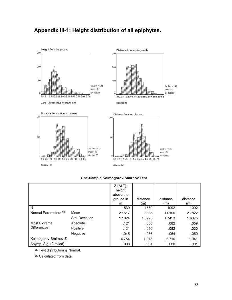
83
Appendix III-1: Height distribution of all epiphytes.
Z (ALT), height above the ground in m
7.06.56.05.55.04.54.03.53.02.52.01.51.0.50.0
Height from the ground
300
200
100
0
Std. Dev = 1.18
Mean = 2.2
N = 1539.00
distance (m)
6.56.05.55.04.54.03.53.02.52.01.51.0.50.0-.5-1.0-1.5-2.0-2.5
Distance from undergrowth
300
200
100
0
Std. Dev = 1.40
Mean = .8
N = 1539.00
distance (m)
6.05.04.03.02.01.00.0-1.0-2.0-3.0-4.0
Distance from bottom of crowns
200
100
0
Std. Dev = 1.75
Mean = 1.0
N = 1092.00
distance (m)
7.56.55.54.53.52.51.5.5-.5-1.5-2.5-3.5
Distance from top of crown
200
100
0
Std. Dev = 1.64
Mean = 2.8
N = 1092.00
One-Sample Kolmogorov-Smirnov Test
1539 1539 1092 1092
2.1517 .8335 1.0100 2.7822
1.1824 1.3995 1.7453 1.6375
.121 .050 .082 .059
.121 .050 .082 .030
-.045 -.036 -.064 -.059
4.754 1.978 2.710 1.941
.000 .001 .000 .001
N
Mean
Std. Deviation
Normal Parameters a,b
Absolute
Positive
Negative
Most Extreme
Differences
Kolmogorov-Smirnov Z
Asymp. Sig. (2-tailed)
Z (ALT),
height
above the
ground in
m
distance
(m)
distance
(m)
distance
(m)
Test distribution is Normal.a.
Calculated from data.b.
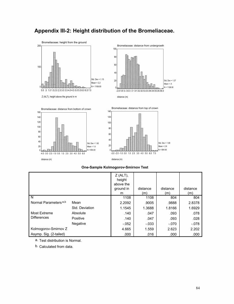
84
Appendix III-2: Height distribution of the Bromeliaceae.
Z (ALT), height above the ground in m
7.06.56.05.55.04.54.03.53.02.52.01.51.0.50.0
Bromeliaceae: height from the ground
200
100
0
Std. Dev = 1.15
Mean = 2.2
N = 1108.00
distance (m)
6.05.55.04.54.03.53.02.52.01.51.0.50.0-.5-1.0-1.5-2.0
Bromeliaceae: distance from undergrowth
100
80
60
40
20
0
Std. Dev = 1.37
Mean = .9
N = 1108.00
distance (m)
6.05.04.03.02.01.00.0-1.0-2.0-3.0-4.0
Bromeliaceae: distance from bottom of crown
160
140
120
100
80
60
40
20
0
Std. Dev = 1.82
Mean = 1.0
N = 804.00
distance (m)
7.06.05.04.03.02.01.00.0-1.0-2.0-3.0
Bromeliaceae: distance from top of crown
140
120
100
80
60
40
20
0
Std. Dev = 1.69
Mean = 2.8
N = 804.00
One-Sample Kolmogorov-Smirnov Test
1108 1108 804 804
2.2092 .9005 .9888 2.8378
1.1545 1.3688 1.8166 1.6929
.140 .047 .093 .078
.140 .047 .093 .028
-.052 -.033 -.070 -.078
4.665 1.559 2.623 2.202
.000 .016 .000 .000
N
Mean
Std. Deviation
Normal Parameters a,b
Absolute
Positive
Negative
Most Extreme
Differences
Kolmogorov-Smirnov Z
Asymp. Sig. (2-tailed)
Z (ALT),
height
above the
ground in
m
distance
(m)
distance
(m)
distance
(m)
Test distribution is Normal.a.
Calculated from data.b.

85
Appendix III-3: Height distribution of the Orchidaceae.
Z (ALT), height above the ground in m
5.04.54.03.53.02.52.01.51.0.50.0
Orchidaceae: height from the ground
40
30
20
10
0
Std. Dev = 1.02
Mean = 1.8
N = 346.00
distance (m)
4.03.53.02.52.01.51.0.50.0-.5-1.0-1.5-2.0
Orchidaceae: distance from undergrowth
40
30
20
10
0
Std. Dev = 1.28
Mean = .5
N = 346.00
distance (m)
6.56.05.55.04.54.03.53.02.52.01.51.0.50.0-.5-1.0-1.5
Orchidaceae: distance from bottom of crown
50
40
30
20
10
0
Std. Dev = 1.45
Mean = 1.2
N = 245.00
distance (m)
7.06.56.05.55.04.54.03.53.02.52.01.51.0.50.0-.5
Orchidaceae: distance from top of crown
40
30
20
10
0
Std. Dev = 1.40
Mean = 2.8
N = 245.00
One-Sample Kolmogorov-Smirnov Test
346 346 245 245
1.8368 .5060 1.2023 2.7919
1.0240 1.2752 1.4510 1.3969
.060 .053 .097 .057
.060 .053 .097 .057
-.046 -.042 -.046 -.030
1.110 .981 1.511 .895
.170 .291 .021 .400
N
Mean
Std. Deviation
Normal Parameters a,b
Absolute
Positive
Negative
Most Extreme
Differences
Kolmogorov-Smirnov Z
Asymp. Sig. (2-tailed)
Z (ALT),
height
above the
ground in
m
distance
(m)
distance
(m)
distance
(m)
Test distribution is Normal.a.
Calculated from data.b.

86
Appendix III-4: Height distribution of the Loranthaceae.
Z (ALT), height above the ground in m
7.06.56.05.55.04.54.03.53.02.52.01.51.0.5
Loranthaceae: height from the ground
30
20
10
0
Std. Dev = 1.77
Mean = 2.8
N = 75.00
distance (m)
6.56.05.55.04.54.03.53.02.52.01.51.0.50.0-.5-1.0-1.5-2.0-2.5
Loranthaceae: distance from undergrowth
20
10
0
Std. Dev = 1.97
Mean = 1.4
N = 75.00
distance (m)
3.02.52.01.51.0.50.0-.5-1.0-1.5-2.0-2.5-3.0-3.5
Loranthaceae: distance from bottom of crown
10
8
6
4
2
0
Std. Dev = 1.90
Mean = .1
N = 34.00
distance (m)
5.04.03.02.01.00.0-1.0-2.0-3.0
Loranthaceae: distance from top of crown
10
8
6
4
2
0
Std. Dev = 1.63
Mean = 1.6
N = 34.00
One-Sample Kolmogorov-Smirnov Test
75 75 34 34
2.8303 1.4343 .1185 1.6394
1.7703 1.9670 1.8992 1.6330
.209 .183 .172 .129
.209 .183 .172 .129
-.135 -.103 -.137 -.076
1.813 1.588 1.003 .755
.003 .013 .267 .619
N
Mean
Std. Deviation
Normal Parameters a,b
Absolute
Positive
Negative
Most Extreme
Differences
Kolmogorov-Smirnov Z
Asymp. Sig. (2-tailed)
Z (ALT),
height
above the
ground in
m
distance
(m)
distance
(m)
distance
(m)
Test distribution is Normal.a.
Calculated from data.b.
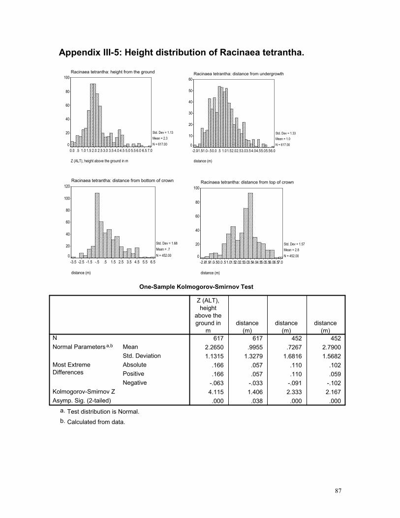
87
Appendix III-5: Height distribution of Racinaea tetrantha.
Z (ALT), height above the ground in m
7.06.56.05.55.04.54.03.53.02.52.01.51.0.50.0
Racinaea tetrantha: height from the ground
100
80
60
40
20
0
Std. Dev = 1.13
Mean = 2.3
N = 617.00
distance (m)
6.05.55.04.54.03.53.02.52.01.51.0.50.0-.5-1.0-1.5-2.0
Racinaea tetrantha: distance from undergrowth
60
50
40
30
20
10
0
Std. Dev = 1.33
Mean = 1.0
N = 617.00
distance (m)
6.55.54.53.52.51.5.5-.5-1.5-2.5-3.5
Racinaea tetrantha: distance from bottom of crown
120
100
80
60
40
20
0
Std. Dev = 1.68
Mean = .7
N = 452.00
distance (m)
7.06.56.05.55.04.54.03.53.02.52.01.51.0.50.0-.5-1.0-1.5-2.0
Racinaea tetrantha: distance from top of crown
100
80
60
40
20
0
Std. Dev = 1.57
Mean = 2.8
N = 452.00
One-Sample Kolmogorov-Smirnov Test
617 617 452 452
2.2650 .9955 .7267 2.7900
1.1315 1.3279 1.6816 1.5682
.166 .057 .110 .102
.166 .057 .110 .059
-.063 -.033 -.091 -.102
4.115 1.406 2.333 2.167
.000 .038 .000 .000
N
Mean
Std. Deviation
Normal Parameters a,b
Absolute
Positive
Negative
Most Extreme
Differences
Kolmogorov-Smirnov Z
Asymp. Sig. (2-tailed)
Z (ALT),
height
above the
ground in
m
distance
(m)
distance
(m)
distance
(m)
Test distribution is Normal.a.
Calculated from data.b.

88
Appendix III-6: Height distribution of Tillandsia compacta
Z (ALT), height above the ground in m
5.55.04.54.03.53.02.52.01.51.0.50.0
Tillandsia compacta: height from the ground
30
20
10
0
Std. Dev = 1.23
Mean = 2.3
N = 102.00
distance (m)
4.54.03.53.02.52.01.51.0.50.0-.5-1.0-1.5
Tillandsia compacta: distance from undergrowth
20
10
0
Std. Dev = 1.38
Mean = 1.0
N = 102.00
distance (m)
6.05.55.04.54.03.53.02.52.01.51.0.50.0-.5-1.0-1.5-2.0-2.5-3.0
Tillandsia compacta: distance from bottom of crown
14
12
10
8
6
4
2
0
Std. Dev = 1.90
Mean = 1.3
N = 67.00
distance (m)
7.57.06.56.05.55.04.54.03.53.02.52.01.51.0.50.0-.5-1.0-1.5-2.0
Tillandsia compacta: distance from top of crown
10
8
6
4
2
0
Std. Dev = 1.99
Mean = 2.9
N = 67.00
One-Sample Kolmogorov-Smirnov Test
102 102 67 67
2.3217 1.0117 1.3149 2.8872
1.2281 1.3753 1.9014 1.9915
.077 .054 .087 .085
.077 .054 .086 .085
-.053 -.050 -.087 -.070
.778 .545 .715 .697
.581 .928 .686 .716
N
Mean
Std. Deviation
Normal Parameters a,b
Absolute
Positive
Negative
Most Extreme
Differences
Kolmogorov-Smirnov Z
Asymp. Sig. (2-tailed)
Z (ALT),
height
above the
ground in
m
distance
(m)
distance
(m)
distance
(m)
Test distribution is Normal.a.
Calculated from data.b.

89
Appendix III-7: Height distribution of Tillandsia sp.1.
Z (ALT), height above the ground in m
6.05.55.04.54.03.53.02.52.01.51.0.50.0
Tillandsia sp.1: height from the ground
70
60
50
40
30
20
10
0
Std. Dev = 1.21
Mean = 2.1
N = 334.00
distance (m)
4.54.03.53.02.52.01.51.0.50.0-.5-1.0-1.5-2.0
Tillandsia sp.1: distance from undergrowth
50
40
30
20
10
0
Std. Dev = 1.45
Mean = .8
N = 334.00
distance (m)
6.05.04.03.02.01.00.0-1.0-2.0-3.0-4.0
Tillandsia sp.1: distance from bottom of crown
60
50
40
30
20
10
0
Std. Dev = 1.86
Mean = 1.2
N = 244.00
distance (m)
6.56.05.55.04.54.03.53.02.52.01.51.0.50.0-.5-1.0-1.5-2.0-2.5-3.0
Tillandsia sp.1: distance from top of crown
50
40
30
20
10
0
Std. Dev = 1.79
Mean = 2.9
N = 244.00
One-Sample Kolmogorov-Smirnov Test
334 334 244 244
2.1208 .7627 1.1988 2.8858
1.2072 1.4535 1.8555 1.7911
.162 .114 .122 .101
.162 .114 .122 .061
-.076 -.070 -.072 -.101
2.969 2.080 1.899 1.584
.000 .000 .001 .013
N
Mean
Std. Deviation
Normal Parameters a,b
Absolute
Positive
Negative
Most Extreme
Differences
Kolmogorov-Smirnov Z
Asymp. Sig. (2-tailed)
Z (ALT),
height
above the
ground in
m
distance
(m)
distance
(m)
distance
(m)
Test distribution is Normal.a.
Calculated from data.b.
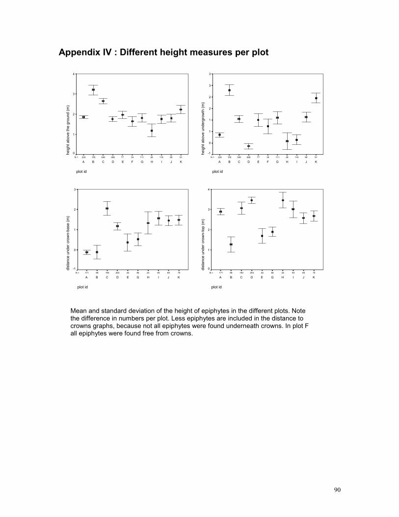
90
Appendix IV : Different height measures per plot
9190116261113477266349155224N =
plot id
KJIHGFEDCBA
height above the ground (m)
4
3
2
1
0
9190116261113477266349155224N =
plot id
KJIHGFEDCBA
height above undergrowth (m)
3
3
2
2
1
1
0
-1
75659324844425319390171N =
plot id
KJIHGEDCBA
distance under crown-base (m)
3
2
1
0
-1
75659324844425319390171N =
plot id
KJIHGEDCBA
distance under crown-top (m)
4
3
2
1
0
Mean and standard deviation of the height of epiphytes in the different plots. Note the difference in numbers per plot. Less epiphytes are included in the distance to crowns graphs, because not all epiphytes were found underneath crowns. In plot F all epiphytes were found free from crowns.

91
Appendix V : Different height measures per species
422193242294213334102617N =
Dendrop. spec
Lor. spec1
Orchid spec5
Orchid spec1
Orchid specs
Brom. specs
R. penlandii
T. spec1
T. compacta
R. tetrantha
height above the ground (m)
5
4
3
2
1
0
422193242294213334102617N =
Dendrop. spec
Lor. spec1
Orchid spec5
Orchid spec1
Orchid specs
Brom. specs
R. penlandii
T. spec1
T. compacta
R. tetrantha
height above undergrowth (m)
3
2
1
0
-1
2385821166311024467452N =
Dendrop.spec
Lor.spec1
Orchidspec5
Orchidspec1
Orchidspecs
Brom.specs
R.penlandii
T.spec1
T.compacta
R.tetrantha
distanceundercrown-top
5
4
3
2
1
0
2385821166311024467452N =
Dendrop. spec
Lor. spec1
Orchid spec5
Orchid spec1
Orchid specs
Brom. specs
R. penlandii
T. spec1
T. compacta
R. tetrantha
distance under crown-base (m)
4
3
2
1
0
-1
-2
Mean and standard deviation of the height of epiphytes per species. Less epiphytes are included in the distance to crowns graphs, because only ca. 2/3 of the epiphytes were found underneath crowns.

92
Appendix VI-1: L2-graphs
L2 PLOT A ( x - y)
-1.00
-0.50
0.00
0.50
1.00
1.50
0 0.3 0.6 0.9 1.2 1.5 1.8 2.1 2.4 2.7
h (m)
L2
L2 Upper
L2
L2 Lower
L2 PLOT A ( x - z )
-1.00
-0.50
0.00
0.50
1.00
1.50
0 0.3 0.6 0.9 1.2 1.5 1.8 2.1 2.4 2.7
h (m)
L2
L2 Upper
L2
L2 Lower
L2 PLOT A ( y- z )
-1.00
-0.50
0.00
0.50
1.00
1.50
0 0.3 0.6 0.9 1.2 1.5 1.8 2.1 2.4 2.7
h (m)
L2
L2 Upper
L2
L2 Lower

93
Appendix VI-2
R. tetrantha, plot A
-1.00
-0.50
0.00
0.50
1.00
1.50
2.00
0 0.3 0.6 0.9 1.2 1.5 1.8 2.1 2.4 2.7
h (m)
L2
L2 Upper
L2
L2 Lower
R. tetrantha adults, plot A
-1.00
-0.50
0.00
0.50
1.00
1.50
2.00
0 0.3 0.6 0.9 1.2 1.5 1.8 2.1 2.4 2.7
h (m)
L2
L2 Upper
L2
L2 Lower
R. tetrantha juveniles, plot A
-1.00
-0.50
0.00
0.50
1.00
1.50
0 0.3 0.6 0.9 1.2 1.5 1.8 2.1 2.4 2.7
h (m)
L2
L2 Upper
L2
L2 Low er
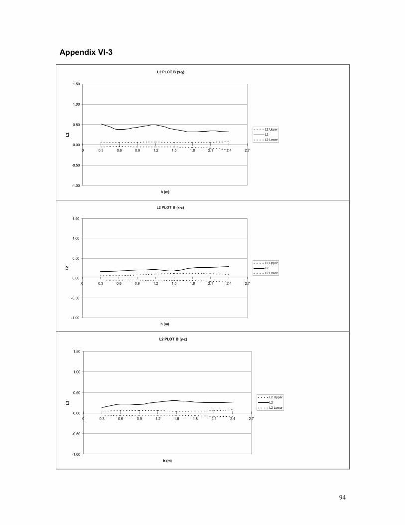
94
Appendix VI-3
L2 PLOT B (x-y)
-1.00
-0.50
0.00
0.50
1.00
1.50
0 0.3 0.6 0.9 1.2 1.5 1.8 2.1 2.4 2.7
h (m)
L2
L2 Upper
L2
L2 Lower
L2 PLOT B (x-z)
-1.00
-0.50
0.00
0.50
1.00
1.50
0 0.3 0.6 0.9 1.2 1.5 1.8 2.1 2.4 2.7
h (m)
L2
L2 Upper
L2
L2 Lower
L2 PLOT B (y-z)
-1.00
-0.50
0.00
0.50
1.00
1.50
0 0.3 0.6 0.9 1.2 1.5 1.8 2.1 2.4 2.7
h (m)
L2
L2 Upper
L2
L2 Lower
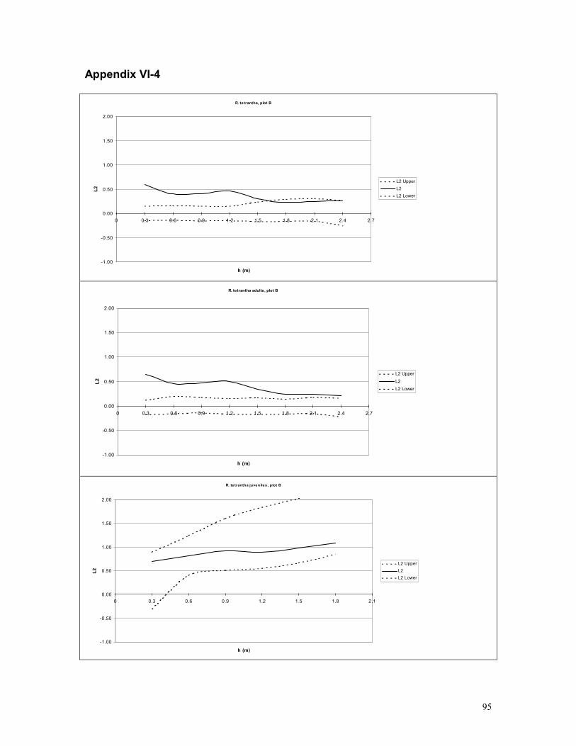
95
Appendix VI-4
R. tetrantha, plot B
-1.00
-0.50
0.00
0.50
1.00
1.50
2.00
0 0.3 0.6 0.9 1.2 1.5 1.8 2.1 2.4 2.7
h (m)
L2
L2 Upper
L2
L2 Lower
R. tetrantha adults, plot B
-1.00
-0.50
0.00
0.50
1.00
1.50
2.00
0 0.3 0.6 0.9 1.2 1.5 1.8 2.1 2.4 2.7
h (m)
L2
L2 Upper
L2
L2 Lower
R. te trantha juveniles, plot B
-1.00
-0.50
0.00
0.50
1.00
1.50
2.00
0 0.3 0.6 0.9 1.2 1.5 1.8 2.1
h (m)
L2
L2 Upper
L2
L2 Lower

96
Appendix VI-5
R. tetrantha, plot C
-1.00
-0.50
0.00
0.50
1.00
1.50
2.00
0 0.3 0.6 0.9 1.2 1.5 1.8 2.1 2.4 2.7
h (m)
L2
L2 Upper
L2
L2 Lower
R. tetrantha adults, plot C
-1.00
-0.50
0.00
0.50
1.00
1.50
2.00
0 0.3 0.6 0.9 1.2 1.5 1.8 2.1 2.4 2.7
h (m)
L2
L2 Upper
L2
L2 Low er
R. tetrantha juveniles, plot C
-1.00
-0.50
0.00
0.50
1.00
1.50
2.00
0 0.3 0.6 0.9 1.2 1.5 1.8 2.1 2.4 2.7
h (m)
L2
L2 Upper
L2
L2 Low er
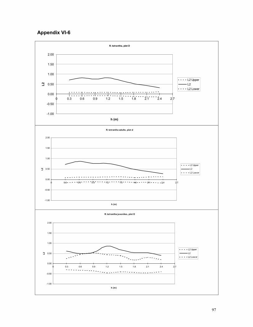
97
Appendix VI-6
R. tetrantha, plot D
-1.00
-0.50
0.00
0.50
1.00
1.50
2.00
0 0.3 0.6 0.9 1.2 1.5 1.8 2.1 2.4 2.7
h (m)
L2
L2 Upper
L2
L2 Lower
R. tetrantha adults, plot d
-1.00
-0.50
0.00
0.50
1.00
1.50
2.00
0 0.3 0.6 0.9 1.2 1.5 1.8 2.1 2.4 2.7
h (m)
L2
L2 Upper
L2
L2 Low er
R. tetrantha juveniles, plot D
-1.00
-0.50
0.00
0.50
1.00
1.50
2.00
0 0.3 0.6 0.9 1.2 1.5 1.8 2.1 2.4 2.7
h (m)
L2
L2 Upper
L2
L2 Low er

98
Appendix VI-7
L2 PLOT E (y-z)
-1.00
-0.50
0.00
0.50
1.00
1.50
0 0.3 0.6 0.9 1.2 1.5 1.8 2.1 2.4 2.7
h (m)
L2 Upper
L2
L2 Lower
L2 PLOT E (x-z)
-1.00
-0.50
0.00
0.50
1.00
1.50
0 0.3 0.6 0.9 1.2 1.5 1.8 2.1 2.4 2.7
h (m)
L2 Upper
L2
L2 Lower
L2 PLOT E (y-z)
-1.00
-0.50
0.00
0.50
1.00
1.50
0 0.3 0.6 0.9 1.2 1.5 1.8 2.1 2.4 2.7
h (m)
L2
L2 Upper
L2
L2 Lower
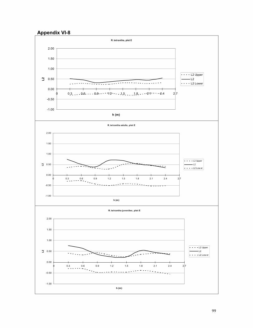
99
Appendix VI-8
R. tetrantha, plot E
-1.00
-0.50
0.00
0.50
1.00
1.50
2.00
0 0.3 0.6 0.9 1.2 1.5 1.8 2.1 2.4 2.7
h (m)
L2
L2 Upper
L2
L2 Lower
R. tetrantha adults , plot E
-1.00
-0.50
0.00
0.50
1.00
1.50
2.00
0 0.3 0.6 0.9 1.2 1.5 1.8 2.1 2.4 2.7
h (m)
L2
L2 Upper
L2
L2 Low er
R. tetrantha juveniles , plot E
-1.00
-0.50
0.00
0.50
1.00
1.50
2.00
0 0.3 0.6 0.9 1.2 1.5 1.8 2.1 2.4 2.7
h (m)
L2
L2 Upper
L2
L2 Low er
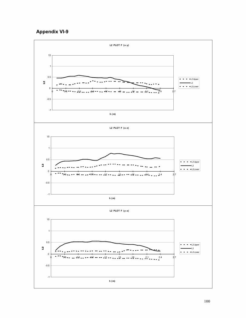
100
Appendix VI-9
L2 PLOT F (x- y)
-1
-0.5
0
0.5
1
1.5
0 0.3 0.6 0.9 1.2 1.5 1.8 2.1 2.4 2.7
h (m)
L2 Upper
L2
L2 Lower
L2 PLOT F (x- z)
-1
-0.5
0
0.5
1
1.5
0 0.3 0.6 0.9 1.2 1.5 1.8 2.1 2.4 2.7
h (m)
L2 Upper
L2
L2 Lower
L2 PLOT F (y- z)
-1
-0.5
0
0.5
1
1.5
0 0.3 0.6 0.9 1.2 1.5 1.8 2.1 2.4 2.7
h (m)
L2 Upper
L2
L2 Lower

101
Appendix VI-10
R. tetrantha, plot F
-1.00
-0.50
0.00
0.50
1.00
1.50
2.00
0 0.3 0.6 0.9 1.2 1.5 1.8 2.1 2.4 2.7
h (m)
L2
L2 Upper
L2
L2 Lower
L2 PLOT G (x-y)
-1.00
-0.50
0.00
0.50
1.00
1.50
0 0.3 0.6 0.9 1.2 1.5 1.8 2.1 2.4 2.7
h (m)
L2
L2 Upper
L2
L2 Lower
L2 PLOT G (x-z)
-1.00
-0.50
0.00
0.50
1.00
1.50
0 0.3 0.6 0.9 1.2 1.5 1.8 2.1 2.4 2.7
h (m)
L2
L2 Upper
L2
L2 Lower
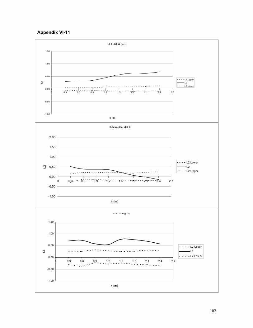
102
Appendix VI-11
L2 PLOT G (y-z)
-1.00
-0.50
0.00
0.50
1.00
1.50
0 0.3 0.6 0.9 1.2 1.5 1.8 2.1 2.4 2.7
h (m)
L2
L2 Upper
L2
L2 Lower
R. tetrantha, plot G
-1.00
-0.50
0.00
0.50
1.00
1.50
2.00
0 0.3 0.6 0.9 1.2 1.5 1.8 2.1 2.4 2.7
h (m)
L2
L2 Lower
L2
L2 Upper
L2 P LOT H ( y - z )
-1.00
-0.50
0.00
0.50
1.00
1.50
0 0.3 0.6 0.9 1.2 1.5 1.8 2.1 2.4 2.7
h (m )
L2
L2 Upper
L2
L2 Low er

103
Appendix VI-12
L2 PLOT H (x-z)
-1.00
-0.50
0.00
0.50
1.00
1.50
0 0.3 0.6 0.9 1.2 1.5 1.8 2.1 2.4 2.7
h (m)
L2
L2 Upper
L2
L2 Low er
L2 PLOT H (y-z)
-1.00
-0.50
0.00
0.50
1.00
1.50
0 0.3 0.6 0.9 1.2 1.5 1.8 2.1 2.4 2.7
h (m)
L2
L2 Upper
L2
L2 Low er
R. tetrantha, plot H
-1.00
-0.50
0.00
0.50
1.00
1.50
2.00
0 0.3 0.6 0.9 1.2 1.5 1.8 2.1 2.4 2.7
h (m)
L2
L2 Upper
L2
L2 Lower
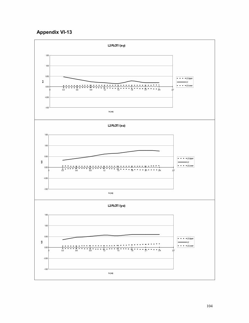
104
Appendix VI-13
L2 PLOT I (x-y)
-1.00
-0.50
0.00
0.50
1.00
1.50
0 0.3 0.6 0.9 1.2 1.5 1.8 2.1 2.4 2.7
h (m)
L2 Upper
L2
L2 Lower
L2 PLOT I (x-z)
-1.00
-0.50
0.00
0.50
1.00
1.50
0 0.3 0.6 0.9 1.2 1.5 1.8 2.1 2.4 2.7
h (m)
L2 Upper
L2
L2 Lower
L2 PLOT I (y-z)
-1.00
-0.50
0.00
0.50
1.00
1.50
0 0.3 0.6 0.9 1.2 1.5 1.8 2.1 2.4 2.7
h (m)
L2 Upper
L2
L2 Lower

105
Appendix VI-14
R. tetrantha, plot I
-1.00
-0.50
0.00
0.50
1.00
1.50
2.00
0 0.3 0.6 0.9 1.2 1.5 1.8 2.1 2.4 2.7
h (m)
L2
L2 Upper
L2
L2 Lower
L2 PLOT J (x-y)
-1.00
-0.50
0.00
0.50
1.00
1.50
0 0.3 0.6 0.9 1.2 1.5 1.8 2.1 2.4 2.7
h (m)
L2
L2 Upper
L2
L2 Lower
L2 PLOT J (x-z)
-1.00
-0.50
0.00
0.50
1.00
1.50
0 0.3 0.6 0.9 1.2 1.5 1.8 2.1 2.4 2.7
h (m)
L2
L2 Upper
L2
L2 Lower
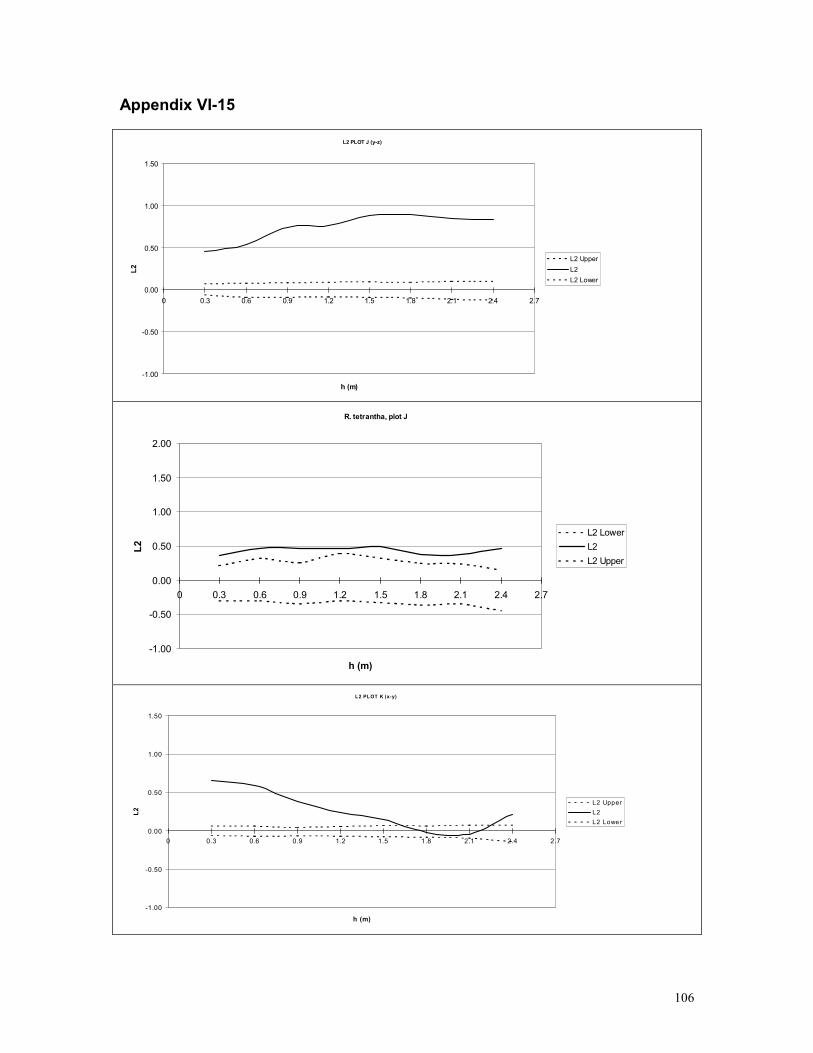
106
Appendix VI-15
L2 PLOT J (y-z)
-1.00
-0.50
0.00
0.50
1.00
1.50
0 0.3 0.6 0.9 1.2 1.5 1.8 2.1 2.4 2.7
h (m)
L2
L2 Upper
L2
L2 Lower
R. tetrantha, plot J
-1.00
-0.50
0.00
0.50
1.00
1.50
2.00
0 0.3 0.6 0.9 1.2 1.5 1.8 2.1 2.4 2.7
h (m)
L2
L2 Lower
L2
L2 Upper
L2 PLOT K (x-y)
-1.00
-0.50
0.00
0.50
1.00
1.50
0 0.3 0.6 0.9 1.2 1.5 1.8 2.1 2.4 2.7
h (m)
L2
L2 Upper
L2
L2 Lower

107
Appendix VI-16
L2 PLOT K (x-z )
-1.00
-0.50
0.00
0.50
1.00
1.50
0 0.3 0.6 0.9 1.2 1.5 1.8 2.1 2.4 2.7
h (m)
L2
L2 Upper
L2
L2 Lower
L2 PLOT K (y-z )
-1.00
-0.50
0.00
0.50
1.00
1.50
0 0.3 0.6 0.9 1.2 1.5 1.8 2.1 2.4 2.7
h (m)
L2
L2 Upper
L2
L2 Lower
R. tetrantha, plot K
-1.00
-0.50
0.00
0.50
1.00
1.50
2.00
0 0.3 0.6 0.9 1.2 1.5 1.8 2.1 2.4 2.7
h (m)
L2
L2 Upper
L2
L2 Lower

108
Appendix VII-1 : Distribution on phorophytes
Tree-species in the graphs: Miconia squamulosa (Melastomataceae), Clethra sp.
(Clethraceae), Miconia thaezans (Melastomataceae), Weinmannia pubescens
(Cunoniaceae), Escallonia myrtilloides (Saxifragaceae), Miconia pergamentacea
(Melastomataceae), Weinmannia sp. (Cunoniaceae), Tibouchina grossa
(Melastomataceae), Hedyosmum sp. (Chloranthaceae), rest = other species, other =
epiphytes on shrubs, on the ground etc.
Epiphytes per host tree species
Tree species
other
dead tree
rest
Hedyosm
um spec.
T. grossa
Weinmannia spec.
M. pergam
entacea
E. myrtilloides
W. pubes
cens
M. thae
zans
Clethra spec.
M. squam
ulosa
# of epiphytes
600
500
400
300
200
100
0
N=1536
Orchids per host tree species
Tree species
other
dead tree
restHedyosm
um spec.
T. grossa
Weinmannia spec
M. pergam
entacea
E. myrtilloides
W. pubes
cens
M. thae
zans
Clethra spec.
M. squam
ulosa
# of orchids
140
120
100
80
60
40
20
0
N=346
Loranthaceae per host tree species
Tree species
other
dead tree
rest
Hedyosm
um spec.
T. grossa
Weinmannia spec.
M. pergam
entacea
E. myrtilloides
W. pubes
cens
M. thae
zans
Clethra spec.
M. squam
ulosa
# Loranthaceae
35
30
25
20
15
10
5
0
N=74

109
Appendix VII-2
R. tetrantha per host tree species
Tree species
other
dead tree
restHedyosm
um spec.
T. grossa
Weinmannia spec.
M.pergam
entacea
E. myrtilloides
W. pubes
cens
M. thae
zans
Clethra spec.
M. squam
ulosa
# ramets
175
150
125
100
75
50
25
0
Adults (N=377)
Juveniles (N=238)
R. tetrantha per host tree species
Tree species
other
dead tree
restHedyosm
um spec.
T. grossa
Weinmannia spec.
M. pergam
entacea
E. myrtilloides
W. pubes
cens
M. thae
zans
Clethra spec.
M. squam
ulosa
# of R. tetrantha ramets
250
200
150
100
50
0
N=616
T. spec.1 per host tree species
Tree species
other
dead tree
restHedyosm
um spec.
T. grossa
Weinmannia spec.
M. pergam
entacea
E. myrtilloides
W. pubes
cens
M. thae
zans
Clethra spec.
M. squam
ulosa
# of T.spec.1 ramets
140
120
100
80
60
40
20
0
N=334
T. compacta per host tree species
Tree species
other
dead tree
restHedyosm
um spec.
T. grossa
Weinmannia
spec
M. pergam
entacea
E. myrtilloides
W. pubes
cens
M. thae
zans
Clethra spec.
M. squam
ulosa
# T.compacta ramets
45
40
35
30
25
20
15
10
5
0
N=102
Bromeliaceae per host tree species
host tree species
other
dead tree
restHedyosm
um spec.
T. grossa
Weinmannia spec.
M. pergam
entacea
E. myrtilloides
W. pubes
cens
M. thae
zans
Clethra spec.
M. squam
ulosa
# of bromeliad-ramets
300
200
100
0
adult
juvenile
Bromeliaceae per host tree species
host tree species
other
dead tree
restHedyosm
um spec.
T. grossa
Weinmannia spec.
M. pergam
entacea
E. myrtilloides
W. pubes
cens
M. thae
zans
Clethra spec.
M. squam
ulosa
# of Bromeliaceae
500
400
300
200
100
0

110
Appendix VIII: Cryptogams
Covering of trees by different epiphytic cryptogam-types in 3 height zones. Mosses occur mostly below 1 meter. Lichens were recorded including and excluding crustose species. In both cases the cover of stems by lichens increases with height from the ground, which is mainly caused by an increase of non-crustose species (notably Usnia spec.). Increase of lichen cover including crustose species is not significant (Anova, p>0.1) Frullania is equally abundant at all heights (p>0.05). Bars represent means, error bars 95% confidence intervals.(Tukey post-hoc test used)
b
a a
a b
c