a surface velocity spiral observed with adcp and hf · pdf filea surface velocity spiral...

A surface velocity spiral observed with ADCP and

HF radar in the Tsushima Strait

Y. Yoshikawa,1 T. Matsuno,1 K. Marubayashi,1 and K. Fukudome2

Received 6 April 2006; revised 2 February 2007; accepted 12 March 2007; published 26 June 2007.

[1] The structure of a wind-driven flow in the Tsushima Strait is investigated with mooredacoustic Doppler current profiler (ADCP) and HF radar. Two ADCPs of high and lowacoustic frequencies are simultaneously used to measure velocities in both the surfaceboundary layer and the interior with high resolutions. The velocity relative to an interiorflow in the surface boundary layer is estimated by subtracting the reference velocity(estimated from velocities at greater depths) from a velocity in the surface layer, andcomplex principal component analysis (PCA) of the lagged wind stress and the relativevelocity is performed. Despite a short (2 weeks) observation period of relatively calmand variable wind, a clockwise velocity spiral similar to a theoretical Ekman spiral isdetected as the first mode of PCA. Ekman transport estimated from the relative velocitiesof the first mode agrees best with Ekman transport expected from wind stress of thefirst mode with 11–13 hours time lag, for which the explained variance of the first mode isalso largest. This indicates that a wind-driven flow is balanced with wind stress after11–13 hours, half of the inertial period at this latitude. Eddy viscosity is also inferred fromwind stress and the relative velocities of the first mode. It is found to increase fromO(10�3) m2 s�1 at greater depth to O(10�2) m2 s�1 near the sea surface.

Citation: Yoshikawa, Y., T. Matsuno, K. Marubayashi, and K. Fukudome (2007), A surface velocity spiral observed with ADCP and

HF radar in the Tsushima Strait, J. Geophys. Res., 112, C06022, doi:10.1029/2006JC003625.

1. Introduction

[2] Wind over the Tsushima Strait (Figure 1) is occasion-ally high in summer and always strong in winter. A surfaceboundary flow driven by local wind stress (hereafter referredto as a wind-driven flow) is thus expected to be occasionallylarge in summer and always intense in winter. HF radardeployed in this strait [Yoshikawa et al., 2006] measures asurface current comprising a shallow wind-driven flow andinterior flows such as a geostrophic current (the TsushimaWarmCurrent) and tidal currents. To estimate an interior flowfield from HF radar measurement, the wind-driven velocitymust be separated from a total velocity measured with HFradar.[3] According to the classical linear theory of Ekman

[1905], a steady wind-driven velocity spirals clockwise withdepth in the Northern Hemisphere. Several field studies[Weller, 1981; Price et al., 1986; Stacey et al., 1986;Richmanet al., 1987; Weller et al., 1991; Wijffels et al., 1994;Chereskin, 1995; Lee and Eriksen, 1996; Schudlich andPrice, 1998] found similar velocity spirals in the actualocean. However, some spirals were flatter than the Ekmanspiral; current rotated less with depth than Ekman theory.

Price et al. [1986] showed that diurnal variations of stratifi-cation and eddy viscosity make a velocity spiral flatter asobserved. This demonstrates the crucial importance of eddyviscosity on a detailed structure (spiral) of a wind-drivenflow. However, our knowledge of in situ eddy viscosity isvery limited. This means that a structure of wind-driven flowin the Tsushima Strait cannot be accurately predicted. Thusthe structure needs to be measured and identified.[4] There are many difficulties in measuring a wind-

driven flow in the Tsushima Strait. Very active fisheriesand marine traffic in this strait make a long-period surfacemooring impractical although it is desirable for accuratemeasurement of a wind-driven flow [e.g., Schudlich andPrice, 1998]. Access to the mooring site should be keptavailable during our field observation period in case of anunexpected accident between a moored buoy and ships orboats. This and the limited ability of our small ship do notallow operations in winter during large wave heights causedby strong northwesterly monsoon wind. Thus a wind-drivenflow has to be measured in summer, a season of calm andvariable wind.[5] Our observation period spanned for 2 weeks, from 5 to

21 July 2005. Tomeasure a wind-driven flowwithin a limitedperiod with good accuracy, two acoustic Doppler currentprofilers (ADCPs) of different acoustic frequencies weremoored at the surface in an HF radar measurement area.Principal component analysis (PCA) was performed to detectthe wind-driven flow component covarying with wind stress.The velocity spiral corresponding to a theoretical Ekmanspiral was obtained as the first mode of PCA. In section 2, an

JOURNAL OF GEOPHYSICAL RESEARCH, VOL. 112, C06022, doi:10.1029/2006JC003625, 2007ClickHere

for

FullArticle

1Research Institute for Applied Mechanics, Kyushu University,Fukuoka, Japan.

2Interdisciplinary Graduate School of Engineering Sciences, KyushuUniversity, Fukuoka, Japan.

Copyright 2007 by the American Geophysical Union.0148-0227/07/2006JC003625$09.00

C06022 1 of 14

http://dx.doi.org/10.1029/2006JC003625

outline of our field measurement and data source is described.Expected errors of current velocity and wind stress are shownin section 3.Wind, current, and temperature data are shown insection 4, and the wind-driven flow detected from PCA ispresented in section 5. A component other than the wind-

driven flow and a profile of vertical eddy viscosity inferredfrom the wind-driven flow are discussed in section 6. Finally,concluding remarks are given in section 7.

2. Field Observation and Data Source

2.1. Surface Moored Buoy

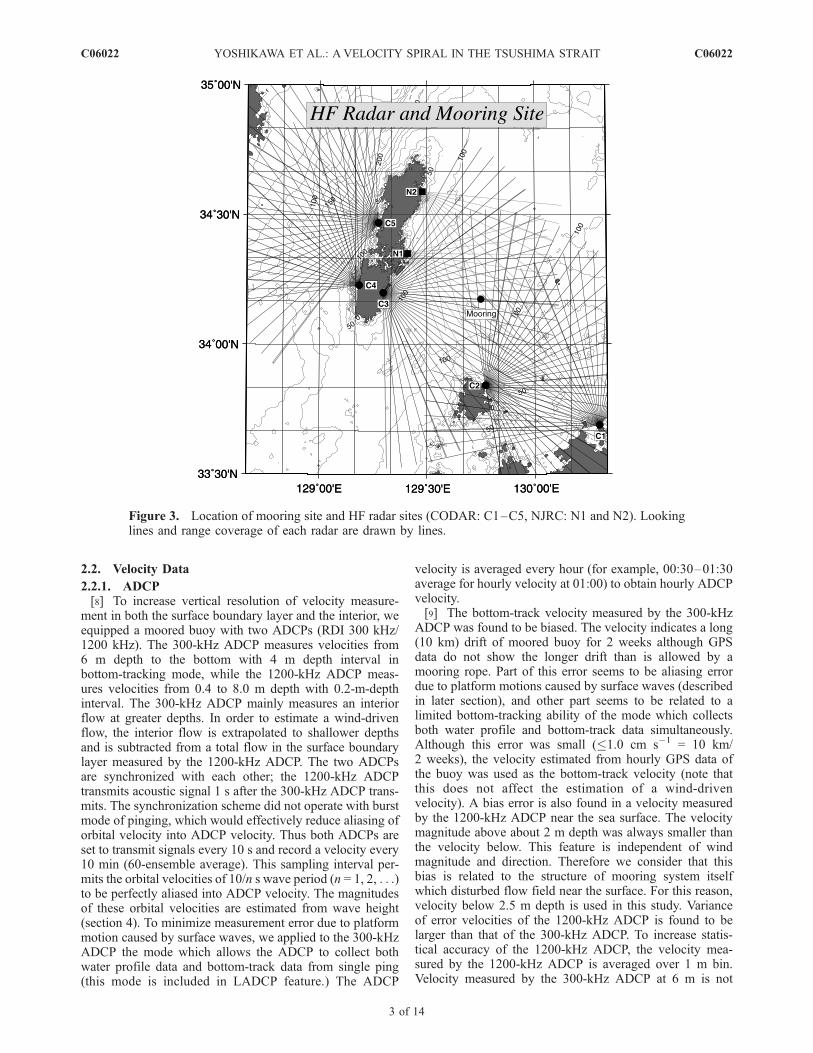
[6] A surface moored buoy as illustrated in Figure 2 wasdeployed on 5 July 2005 by T/V Nagasaki-Maru of NagasakiUniversity. The buoy is anchored at about (34.175�N,129.75�E) in an HF radar measurement area with a 250-mrope where the total water depth is about 100 m (Figure 3).For unexpected drifting of the buoy due to an accident, thebuoy position was tracked every hour by GPS and wassent to laboratory’s PC via e-mail using ORBCOMMsystem.[7] Motion of the buoy is affected by both currents and

surface waves. Figure 4 shows time series of averaged pitch(tilt in the direction of the flow) and roll (tilt in the directiontransverse to the flow) of moored ADCP (averaging intervalis 10 min). Diurnal and semidiurnal oscillations as well ashigher-frequency oscillations are evident. The former oscil-lations are more evident in pitch record, indicating thatstronger tidal current periodically pushed and tilted themoored buoy to a greater degree. The latter oscillationsare due to surface waves. Note that instantaneous pitch androll are expected much larger than averaged ones shown inFigure 4. Surface waves not only stir the platform to increasemeasurement error but also induce large orbital velocity,which acts as noise for our measurement of a wind-drivenflow. Thus surface waves infect ADCPmeasurement, thoughthey are not a major problem in the present analysis, asdescribed in later sections.

Figure 1. Location of the Tsushima Strait (TS). Mooringsite (open triangle), JMA wave height station (Fukuejima;open star), and marine tower station (Tsuyazaki; opencircle) are also indicated.

Figure 2. Schematic illustration of a moored surface buoy. A buoy is composed of 10 dram-shapedfloats, frame of 2.58 m in length and 1.87 m in width, two ADCPs, thermometer, ORBCOMM and GPSsystem, and beacon lights. Transducers of ADCP are set below the level of drum-shaped float’s bottomand about 0.3 m below water level.

C06022 YOSHIKAWA ET AL.: A VELOCITY SPIRAL IN THE TSUSHIMA STRAIT

2 of 14

C06022

2.2. Velocity Data

2.2.1. ADCP[8] To increase vertical resolution of velocity measure-

ment in both the surface boundary layer and the interior, weequipped a moored buoy with two ADCPs (RDI 300 kHz/1200 kHz). The 300-kHz ADCP measures velocities from6 m depth to the bottom with 4 m depth interval inbottom-tracking mode, while the 1200-kHz ADCP meas-ures velocities from 0.4 to 8.0 m depth with 0.2-m-depthinterval. The 300-kHz ADCP mainly measures an interiorflow at greater depths. In order to estimate a wind-drivenflow, the interior flow is extrapolated to shallower depthsand is subtracted from a total flow in the surface boundarylayer measured by the 1200-kHz ADCP. The two ADCPsare synchronized with each other; the 1200-kHz ADCPtransmits acoustic signal 1 s after the 300-kHz ADCP trans-mits. The synchronization scheme did not operate with burstmode of pinging, which would effectively reduce aliasing oforbital velocity into ADCP velocity. Thus both ADCPs areset to transmit signals every 10 s and record a velocity every10 min (60-ensemble average). This sampling interval per-mits the orbital velocities of 10/n s wave period (n = 1, 2, . . .)to be perfectly aliased into ADCP velocity. The magnitudesof these orbital velocities are estimated from wave height(section 4). To minimize measurement error due to platformmotion caused by surface waves, we applied to the 300-kHzADCP the mode which allows the ADCP to collect bothwater profile data and bottom-track data from single ping(this mode is included in LADCP feature.) The ADCP

velocity is averaged every hour (for example, 00:30–01:30average for hourly velocity at 01:00) to obtain hourly ADCPvelocity.[9] The bottom-track velocity measured by the 300-kHz

ADCP was found to be biased. The velocity indicates a long(10 km) drift of moored buoy for 2 weeks although GPSdata do not show the longer drift than is allowed by amooring rope. Part of this error seems to be aliasing errordue to platform motions caused by surface waves (describedin later section), and other part seems to be related to alimited bottom-tracking ability of the mode which collectsboth water profile and bottom-track data simultaneously.Although this error was small (�1.0 cm s�1 = 10 km/2 weeks), the velocity estimated from hourly GPS data ofthe buoy was used as the bottom-track velocity (note thatthis does not affect the estimation of a wind-drivenvelocity). A bias error is also found in a velocity measuredby the 1200-kHz ADCP near the sea surface. The velocitymagnitude above about 2 m depth was always smaller thanthe velocity below. This feature is independent of windmagnitude and direction. Therefore we consider that thisbias is related to the structure of mooring system itselfwhich disturbed flow field near the surface. For this reason,velocity below 2.5 m depth is used in this study. Varianceof error velocities of the 1200-kHz ADCP is found to belarger than that of the 300-kHz ADCP. To increase statis-tical accuracy of the 1200-kHz ADCP, the velocity mea-sured by the 1200-kHz ADCP is averaged over 1 m bin.Velocity measured by the 300-kHz ADCP at 6 m is not

Figure 3. Location of mooring site and HF radar sites (CODAR: C1–C5, NJRC: N1 and N2). Lookinglines and range coverage of each radar are drawn by lines.


3 of 14

C06022

used because its error velocity was exceptionally large. Insummary, ADCP velocities used in this study are at 3 to8 m with 1 m bin size and at 10 m to the bottom with 4 mbin size.2.2.2. HF Radar[10] Two types of HF radar, cross-looped antenna type

(CODAR; C1–C5) and array antenna type with DBFtechnique (NJRC; N1–N2), are installed in the TsushimaStrait (Figure 3). CODAR and NJRC radars transmit 13.9and 24.5 MHz signals to measure an averaged velocity overabout 1.72- and 0.98-m-depth ranges, respectively. A totalof five radars (C1–C3 and N1–N2) measured surfacecurrent at the mooring site. However, comparison withADCP velocity indicates large measurement errors of C1and C3 radars (section 3). For this reason, only N1 and N2(NJRC) radars are used in this study. NJRC is scheduled totransmit signal for 30 min every hour (N1: 44–14 min, N2:46–16 min) and estimates a 30-min averaged velocity thatis used as an hourly HF radar velocity. Further details of

specification of HF radars in the Tsushima Strait aredescribed in the paper of Yoshikawa et al. [2006].2.2.3. Velocity Data Set[11] Hourly velocity data set used in this study is obtained

by simply combining hourly ADCP velocities below 3 mdepth and hourly HF radar velocity at 0.5 m depth. Velocityis thus obtained at 0.5 m depth with 1 m bin size (HF radar),from 3 to 8 m depth with 1 m bin size (the 1200-kHzADCP) and from 10 m depth to the bottom with 4 m binsize (the 300-kHz ADCP). To remove high-frequencycurrent variation (such as tidal currents) from velocity data,a low-pass filter (25 hours running mean) is applied tohourly velocity data. In the following analysis, thesesmoothed hourly velocity data are used.

2.3. Temperature

[12] To measure upper stratification which may affect onthe structure of a wind-driven flow [Price et al., 1986],thermometers were attached with a moored buoy at the seasurface and along a mooring rope at 5, 10, and 30 m distantfrom the surface (water density is mainly determined bytemperature in the observation area). Unfortunately, thedeepest thermometer did not operate appropriately. In thepresent analysis, temperatures measured by upper threethermometers sampled every hour are used.

2.4. Wind Stress

[13] Our buoy was designed to be as light as possible inorder to measure a velocity near the sea surface. Thus ananemometer was not attached. Instead, reanalyzed surfacewind data published by JapanMeteorological Agency (JMA)every 6 hours with 0.125� (longitude) � 0.1� (latitude)resolution (GPV-MSM data) are used in this study. Surfacewind stress is estimated from these wind data with dragcoefficient formula of Yelland and Taylor [1996]. AlthoughYelland and Taylor [1996] formulated the drag coefficientfor wind higher than 3 m s�1, we applied the formula evenwhen the wind speed is lower than 3 m s�1.

2.5. Wave Height of Surface Waves

[14] Surface wave height was not measured at the mooringsite. Instead, it is estimated from wave height measured byJMA at Fukuejima (Figure 1). This station is to the southwestof our mooring site and is the closest (190 km) station amongthe available stations during our field observation. The waveheight is measured for 20 min (35–55 min) every hour with0.25 s interval.

3. Error Estimation

3.1. Variance Error of ADCP Velocity

[15] A variance error of ADCP velocity is first estimatedby comparing the 300-kHz ADCP velocity at 10 m and the1200-kHz ADCP velocity at 8 m (note that a bias error ofADCP velocity is not fully estimated from this comparisonbecause the error might be cancelled when comparing twoADCP velocities). Table 1 shows regression coefficients,correlation, and root mean square (RMS) difference fromthe regression line. Small RMS (1.52 cm s�1) between twovelocities suggests the small variance error of ADCPmeasurement itself. Difference between the bottom-trackvelocity measured by the 300-kHz ADCP (which is notused for an estimation of a wind-driven flow) and the drift

Figure 4. Time series of averaged (a) pitch and (b) roll ofmoored ADCP. Averaging interval is 10 min. Note thedifference in vertical scale between Figures 4a and 4b.


4 of 14

C06022

velocity estimated from hourly GPS data of the buoy can beused to estimate ADCP measurement error. RMS differencebetween the two velocities is 2.28 cm s�1. Note that RMSdifference is larger (3.12 cm s�1) in the strong wind period(8–12 July, average wind magnitude was 6.13 m s�1) andsmaller (1.18 cm s�1) in the weak wind period (14–18 July,average wind magnitude was 2.49 m s�1). This suggeststhat wind and surface waves induce large platform motionsto increase ADCP measurement error. The largest varianceerror of ADCP velocity is thus considered as a fewcentimeters per second.

3.2. Variance Error of HF Radar Velocity

[16] Measurement error of HF radar at the mooring site isexamined by comparing HF radar radial velocity with aradial component of ADCP velocity at 3 m depth (Table 2).Comparisons show very good correlation with C2, N1, andN2 radar velocities. However, large unreasonable varianceerrors are found in C1 and C3 radar velocities. For thisreason, only N1 and N2 (NJRC) radars are used in thisstudy. The RMS difference from the regression line betweenADCP and HF radar velocities is less than 3.08 cm s�1.Since the variance error of ADCP is partly included in thisRMS difference, this can be regarded as a maximum valueof a possible variance error of HF radar radial velocity. Avariance error of velocity vector magnitude is then calcu-lated from a variance error of radial velocity as [Nadai etal., 1999]

sv ¼

ffiffiffiffiffiffiffiffiffiffiffiffiffiffiffiffiffiffiffiffiffiffiffiffiffiffiffi2s2

r

sin2 ðq1 � q2Þ

s;

where sv is a variance error of vector magnitude, sr is avariance error of radial velocity, and q1 � q2 (=30�) is adifference between looking directions from the mooring siteto N1 and N2 sites. A variance error of the vector magnitudeis then estimated to be 8.85 cm s�1.

3.3. Bias Errors of ADCP and HF Radar Velocities

[17] Bias error between HF radar and ADCP velocitiescan be estimated from regression coefficients obtained from

ADCP and HF radar comparison. Slopes of the regressionlines (1.01 and 0.88) are good, and intercepts (5.39 and3.87 cm s�1) seem reasonable if compared with varianceerrors of ADCP and HF radar. It should be noted that theseregression coefficients reflect not only measurement errorsbut also a real difference due to different measurementdepths, different averaging area, and orbital velocity aliasedinto ADCP velocity. Thus regression coefficients are con-sidered to represent maximum values of possible biaserrors of ADCP and HF radar. Yoshikawa et al. [2006]investigated variance and bias errors of HF radar in theTsushima Strait to find that a variance error dominates overa measurement error of HF radar. Mean difference betweenthe bottom-track velocity measured by the 300-kHz ADCPand the drift velocity estimated from hourly GPS data ofthe buoy is also small (0.89 cm s�1). Thus we consider thatbias errors of ADCP and HF radar velocities are reasonablysmall.

3.4. Wind Stress Error

[18] To examine whether the wind stress estimated fromJMA-reanalyzed wind (referred to as JMA wind stress) isappropriate for the present analysis, wind data measured atmarine tower station near the mooring site (Figure 1)operated till 2002 are used. Anemometer at the tower wasattached above about 17 m from the sea surface andmeasured wind for 12 min every hour. The hourly wind isconverted to hourly wind stress using drag coefficientformula of Yelland and Taylor [1996], and a low-pass filter(25 hours running mean) is applied to obtain smoothedhourly wind stress.[19] The smoothed tower wind stress and JMAwind stress

at the tower station are compared (Table 3) from 28 July to27 August 2002 (in which no typhoon hit the tower).Though meridional component of JMA wind stress mightunderestimate that of the tower wind stress by a few 10%,we consider that agreement between two wind stress isrelatively good and that JMAwind stress well represents localwind stress at our mooring site during the field observation.

4. Wind, Current, Water Temperature, andOrbital Velocity

[20] Figure 5 shows hourly wind and current velocities(every 6 hours). Wind is generally weak (3.94 m s�1 onaverage) except in 8–12 July when southerly wind oftenexceeds 10 m s�1 in magnitude. Current generally directs tothe northeast due to the Tsushima Warm Current. Powerspectra of wind stress and hourly current velocities (notshown) show that major part of wind and current energy liesat lower frequencies than the diurnal frequency.[21] Figure 6 shows three typical power spectra of wave

height (P( f )) measured at Fukuejima as a function offrequency ( f ). The spectra show large amplitude of both

Table 1. Comparisons Between 300 kHz ADCP Velocity at 10 m

depth and 1200 kHz ADCP Velocity at 8 m deptha

A B, cm s�1 COR RMS, cm s�1 NUM

Zonal 1.14 �1.03 0.95 1.52 312Meridional 0.97 1.43 0.97 1.43 312

aA andB are slope and intercept of regression line v1200 kHz =Av300 kHz +B,COR is correlation, RMS is root mean square distance from regression line,and NUM is number of samples. Regression line is obtained from PCA.

Table 2. Comparisons Between ADCP-Measured Velocity (at 3 m

depth) and HF Radar-Measured Velocitya

Radar DIS, km A B, cm s�1 COR RMS, cm s�1 NUM

C1 73 0.49 7.27 0.66 4.30 287C2 37 0.70 �0.95 0.87 2.68 331C3 42 0.49 �1.27 0.39 5.95 326N1 37 1.01 5.39 0.91 3.08 349N2 52 0.88 3.87 0.90 3.01 342aDIS is distance between radar site and mooring site. A, B, COR, RMS,

and NUM are same as in Table 1 (vradar = AvADCP + B).

Table 3. Comparisons Between JMA Wind Stress and the Tower

Wind Stressa

A B, Pa COR RMS, Pa NUM

zonal stress 0.92 3.59 � 10�3 0.77 1.07 � 10-2 90meridional stress 1.28 4.32 � 10�3 0.79 1.69 � 10-2 90

aA, B, COR, RMS, and NUM are same as in Table 1 (ttower = AtJMA + B).


5 of 14

C06022

long swell and short wind wave when wind is strong (9 July),small amplitude of both long swell and short wind wavewhen wind is weak (16 July), and large amplitude of onlylong swell when wind is weak (21 July). Thus wave of 10 speriod is composedmostly of long swell, wave of 5 s period iscomposed of both long swell and locally generated shortwind wave, and wave of 2.5 s period is composed mostly ofshort wind wave.[22] Using linear theory, magnitude of total orbital velocity

vorb( f�Df/2: f +Df/2) of the waves in ( f�D f/2, f +D f/2)frequency range at z m depth can be estimated from powerspectrum P( f ) as

vorbð f �Df =2 : f þDf =2Þ ¼ 2pfffiffiffiffiffiffiffiffiffiffiffiffiffiffiffiffiffiPð f ÞDf

pexpð�kzÞ;

where k(= (2pf )2/g) is wave number. Here Df of 2�5 s�1 isused. Magnitude of an aliasing velocity from the waveoutside this frequency range is less than 0.5% of its originalorbital velocity.[23] Time series of the estimated orbital velocity magni-

tudes of 10, 5, and 2.5 s periods are shown in Figure 7. Thevelocity of 2.5 s period is quite small due to small energyand short vertical length scale. The velocity of 5 s period isabout 7 cm s�1 for 8–12 July when wind is strong andotherwise less than a few centimeters per second. The

velocity of long swell (10 s period) is about 5 cm s�1 for8–12 July and after 20 July.[24] Note that the above orbital velocities are all aliased

into hourly ADCP velocity only if direction of wavepropagation is unique and constant during 1 hour. Because

Figure 5. Hourly wind and current velocities during our field observation. Sampling interval is 6 hours.

Figure 6. Power spectrum of wave height measured atFukuejima station (JMA).


6 of 14

C06022

actual direction is neither unique nor constant, the velocitymagnitude that is aliased into ADCP velocity would besmaller than 10 cm s�1. In this study, a maximum value of apossible aliasing velocity is considered to be 10 cm s�1.[25] Figure 8 shows water temperatures measured by

upper three thermometers. Temperatures increase graduallyduring our observation period. Diurnal variation of temper-ature is evident, but diurnal variation of thermal stratifica-tion is not clearly found. In particular, thermal stratificationis negligible on 9–16 July. This is due probably to strongvertical mixing by the intense wind on 8–12 July.

5. Wind-Driven Velocity Structure

5.1. Relative Velocity

[26] To extract a wind-driven velocity from the observed(total) velocity, the velocity of an interior flow (referred toas a reference flow) is subtracted from a total velocity. Thereference flow in the surface boundary layer is estimatedfrom velocities at greater depths where a wind-driven flowis assumed to be negligibly small. The present analysisdepends largely on the estimation of the reference flow.Sensitivities of the estimation on the present analysis will bedescribed in later subsection, and the result with the mostappropriate reference flow is presented in this subsection.[27] The reference flow here is assumed to be linearly

sheared and is estimated by extrapolating a velocity at 18 mdepth to shallower depths with vertical shear averaged over18- to 58-m-depth range. Subtraction of this referencevelocity from a total velocity is expected to yield thevelocity representing a wind-driven flow (referred to as arelative velocity or flow).[28] Figure 9 shows hourly wind stress and the relative

velocity (every 6 hours). The relative velocity is found torotate clockwise with depth particularly in the period of

strong wind stress (8–12 July). However, the relativevelocity is large even in a weak wind stress period (before7 July and after 13 July). This indicates that componentsother than the wind-driven flow covarying with wind stress,such as orbital velocity due to surface waves (particularlylong swell), the flow triggered by wind stress but neitherbalanced with wind stress nor dissipated, and a baroclinicinterior current with higher order vertical shear, are includedin the relative velocity defined above. Although thesecomponents are expected to reduce in magnitude by long-time averaging [Schudlich and Price, 1998], record lengthof velocity data is too short in this study.

5.2. Complex Principal Component Analysis

[29] To extract the wind-driven flow covarying with time-varying wind stress from the relative flow defined above,we perform complex PCA [or empirical orthogonal functionanalysis; Kundu and Allen, 1976] of both the wind stressand the relative velocity during the whole observationperiod. Explained variance and a corresponding set ofvectors (the wind stress and the relative velocity writtenin the complex form) of the first mode are obtained as thelargest eigenvalue and the corresponding eigenvector of(complex) covariance matrix C ¼ W*TW, respectively,where W = (w1,w2,. . .,wK) and wk (k = 1, . . . , K) is anN-element row vector (N is the number of sampling time)of wind stress (k = 1) and relative velocities (2 � k � K).Conjugate transpose matrix of W is represented by W*T.[30] Two normalizations are applied to wk. First, wind

stress and the relative velocity are normalized by root meansquares of wind stress and the shallowest relative velocity(measured by HF radar), respectively. Second, wind stress ismultiplied by (K � 1), the number of levels of the relativevelocities. By this normalization, the first mode is forced tomainly explain wind stress variance. The relative velocitiesof the first mode thus represent the velocity componentcovarying with wind stress. The second normalizationenables the extraction of only the velocity component of

Figure 7. Orbital velocity magnitude vorb( f � Df/2 : f +Df/2) at 3 m depth estimated from wave height spectrumusing linear short-wave theory. The velocity represents totalorbital velocity of the waves in ( f � Df/2, f + Df/2)frequency range (Df = 2�5 s�1). Black line: velocity of 5 swave period (both long swell and short wave). Gray line:velocity of 10 s wave period (long swell). Gray dashed line:velocity of 2.5 s period (short wave).

Figure 8. Time series of water temperatures at the seasurface (black line) and at 5 m (dark gray line) and 10 m(light gray line) distant from the surface along a mooringrope.


7 of 14

C06022

relative velocity covarying with wind stress from totalrelative velocity.[31] Normalized vector wk is thus written as

w1 ¼K � 1

RMSðtn0x ; tn0y Þ

t10

x þ it10

y

t20

x þ it20

y

..

.

0BB@

1CCA;

w2 ¼1

RMSðun0:5m; vn0:5mÞ

u10:5m þ iv10:5mu20:5m þ iv20:5m

..

.

0B@

1CA;

..

.:

RMSðxn; ynÞ ¼ffiffiffiffiffiffiffiffiffiffiffiffiffiffiffiffiffiffiffiffiffiffiffiffiffiffiffiffiffiffiffiffiffiffiffiffiffiffiSN

n¼1xn2 þ yn2

�=N

q �

where i is the imaginary unit, (txn0, ty

n0,) is the hourly windstress at n0 = n � h hour, h is the time lag between wind andcurrent, and (uz m

n ,vz mn ) is the hourly relative velocity

measured at z m at n hour by HF radar (z = 0.5 m) or ADCP(z 3 m). An adjustment of a wind-driven flow to windstress is expected to take time, so that time lag (h) isintroduced in this analysis. Note that wind stress is availableonly every 6 hours, so the hourly relative velocity is usedwhen (lagged) wind stress is available.

5.3. The First Mode

[32] Two parameters, the reference flow and a time lagbetween the wind stress and the relative flow, must bespecified before performing PCA. The reference velocityused in this subsection is the same as in the previoussubsection, and the time lag is set to 11 hours since theseparameters provide the most appropriate estimation ofEkman transport as described later.[33] Figure 10 shows the velocity structure of the first

mode. This mode explains 95.8% of the normalized vari-ance. A high proportion of the first mode is due to thesecond normalization; the first mode is forced to explainwind stress variance to which much weight is given.[34] The first mode seems to represent an Ekman spiral

balanced to the local wind stress at 11 hours ago. Figure 11

shows vertical profiles of velocity magnitude and directionof the first mode and those of an Ekman solution obtainedwith uniform eddy viscosity of 5.0 � 10�3 m2 s�1. Avelocity profile of the first mode is less smooth than thetheoretical one. A velocity magnitude of the first mode issmaller than that of theoretical one near the surface dueprobably to large eddy viscosity near the surface (section 6).On the other hand, a velocity of the first mode rotates asmuch as the theoretical one. This is in contrast to previousstudies in which a velocity spiral is flatter than Ekmantheory. Price et al. [1986] showed the importance of diurnal

Figure 9. Hourly wind stress (red) and hourly relative velocities (blue to green). Color legends for therelative velocities are shown in the figure. Data are plotted only when both wind stress (obtained every6 hours) and relative velocities are obtained.

Figure 10. (a) Wind stress and relative velocities of the firstmode. Color legends are same as in Figure 9. (b) Ekmantransport estimated from integration of the relative velocitiesof the first mode (blue) and Ekman transport expected fromthe wind stress of the first mode (red). Wind stress is set topoint to the north.


8 of 14

C06022

cycle of stratification on flat spiral formation. In ourobservation period, stratification is negligibly small duringstrong wind (Figure 8). This is the most probable cause ofless flat spiral in this study. Velocity magnitude and direc-tion at 3–5 and 6–8 m group together, respectively, as ifthere are slab sublayers of 3 m thickness at these depths.[35] Figure 10 also shows the Ekman transport estimated

from integration of the relative velocities of the first mode(referred to as the estimated Ekman transport) and thetransport expected from the wind stress of the first mode(referred to as the expected Ekman transport). Very goodagreement between two transports suggests Ekman balancebetween the wind stress and the relative velocities of thefirst mode.[36] Figure 12 shows time series of the (lagged) wind stress

and the relative velocities (upper panel), those of the firstmode (middle panel), and those of the higher modes (lowerpanel). It is clear that the velocity component covarying withwind stress is successfully extracted from the total relativevelocity (upper panel) as the first mode (middle panel). Thefirst mode, however, explains only 28.9% of the ‘‘current’’velocity variance (Sk = 2

K |wk|2). This is because much weight

is attached to wind stress, and hence the first mode is selectedto explain first the wind stress variance. This also indicatesthat velocity component not covarying with wind stressdominates the relative velocity variance. Sources of thiscomponent are discussed in section 6.

5.4. Sensitivity to Reference Flow

[37] The simplest definition of the reference flow is toassume a vertically uniform (barotropic) interior flow as inthe previous studies. In this definition, a reference depth(whose velocity is set to a velocity of the uniform referenceflow) is only parameter to be specified. Table 4 shows the

estimated and the expected Ekman transport for severalreference depths. The most appropriate reference depth isfound to be 18 m although there remains difference indirection between two transports.[38] A second simple definition of the reference flow is to

assume a linearly sheared interior flow. In this definition,not only the reference depth but also (uniform) the verticalshear of the reference flow (referred to as a reference shear)must be specified to extrapolate a velocity at the referencedepth. Although there are many possible definitions of thereference shear, the most appropriate one will be the shearaveraged over a certain depth range just below the referencedepth. In this case, the parameters to be examined are thereference depth and the depth range over which averagedshear is estimated.[39] Several reference depths and average depth ranges

are examined (Table 4). It is found that very good agree-ment between the estimated and the expected Ekmantransport is obtained for the reference depth of 18 m andthe average depth range of 40 m.

5.5. Sensitivity to Time Lag

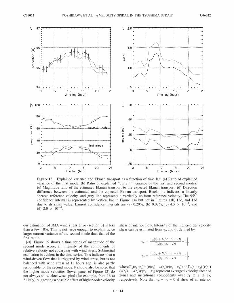
[40] Figure 13 shows the ratio of explained variance tototal variance (score) of the first mode, the ratio ofexplained ‘‘current’’ variance to total ‘‘current’’ varianceof the first and second modes, the magnitude ratio of theestimated Ekman transport to the expected one, and thedirection difference between the estimated and the expectedEkman transport as a function of time lag. The 95%confidence intervals estimated from variance errors ofADCP and HF radar velocity (Appendix) are also shownin Figure 13. Here variance error of HF radar velocity is setto 8.85 cm s�1 (section 3) and that of ADCP velocity is setto 10 cm s�1, taking into account the possible aliasing oforbital velocity due to surface waves (section 4).[41] In this subsection, the linearly sheared reference flow

with the reference depth of 18 m and the average depthrange for the reference shear of 40 m is assumed. Ratio ofexplained variance of the first mode is 94.9% without timelag and increases gradually to be largest (95.6–95.8%) for10- to 17-hour time lags. Ratio of explained ‘‘current’’variance of the first mode also shows similar change withtime lag and is largest (28.4–29.6%) for 11- to 13-hour timelags, for which ratio of explained ‘‘current’’ variance of thesecond mode is smallest (60.7–62.1%). A magnitude of theestimated Ekman transport is closest (within a 2.06%difference) to that of the expected Ekman transport for 11-to 13-hour time lags. Direction difference between thetransports is also smallest (0.44�–3.08�) for these time lags.All these results suggest that the wind-driven flow isbalanced with a wind stress after 11–13 hours, whichcorresponds to half of the inertial period (21.5 hours).[42] Note that wind stress error and possible bias errors of

ADCP and HF radar velocities are not considered in thepresent analysis. In particular, the orbital velocity due toshort wind waves, which will covary with wind stress,might be aliased into hourly ADCP velocity of the firstmode, although the aliased velocity will be much less than7 cm s�1 (Figure 7), which is estimated as the largest velocityunder the assumption of a unique and constant direction ofwave propagation (section 4). Taking into account thispossible errors and aliasing velocity, it should be considered

Figure 11. Vertical profile of velocity magnitude (solidcircle) and direction (open square) of the first mode (solid line)and an Ekman solution (dashed line) calculated with verticaleddy viscosity of 5 � 10�3 m2 s�1. Dotted line representse-folding depth scale calculated from magnitude of therelative velocities. Wind stress is set to point to the north.


9 of 14

C06022

that the discrepancy in the Ekman transports for the moretraditional approach (vertical uniform reference flow andzero time lag) is also small.

6. Discussion

6.1. The Second Mode

[43] The major part of the velocity components not cova-rying with wind stress is represented by the second mode. It

explains only 3.68% of total normalized variance (Sk = 1K |wk|

2)but 62.1% of ‘‘current’’ variance (Sk = 2

K |wk|2). Possible

sources of the second mode are discussed in this subsection.[44] Figure 14 shows the velocity structure of the second

mode. Noteworthy is that the second mode shows clock-wise velocity spiral with depth. This suggests that thesecond mode represents the mismatch between the actualwind stress and the JMA wind stress estimated fromreanalyzed wind and drag coefficient formula. However,

Figure 12. Time series of wind stress and relative velocities. Upper: total wind stress and relativevelocities. Middle: wind stress and relative velocities of the first mode. Lower: wind stress and relativevelocities of higher modes than the first. Color legends are same as in Figure 9.

Table 4. Comparisons Between the Estimated and the Expected Ekman Transporta

U

S

D = 24 m D = 32 m D = 40 m D = 48 m D = 56 m

zr, m r Dq, � r Dq, � r Dq, � r Dq, � r Dq, � r Dq, �

10 0.42 42.5 0.29 41.814 0.88 25.8 0.70 15.218 1.18 16.5 0.89 �3.4 0.97 �1.4 1.01 0.4 1.00 3.0 1.01 5.222 1.50 18.4 1.27 1.726 1.89 24.6 1.54 9.5aU indicates a uniform reference flow, and S indicates a linearly sheared reference flow. zr is the reference depth, D is the

averaging depth (the reference shear is estimated from average velocity shear between zr and zr + D), r is the magnitude ratio ofthe estimated to the expected Ekman transport, and Dq is the direction difference between the estimated and the expectedEkman transport. Time lag of 11 hours is assumed.


10 of 14

C06022

our estimation of JMA wind stress error (section 3) is lessthan a few 10%. This is not large enough to explain twicelarger current variance of the second mode than that of thefirst mode.[45] Figure 15 shows a time series of magnitude of the

second mode score, an intensity of the components ofrelative velocity not covarying with wind stress. Subinertialoscillation is evident in the time series. This indicates that awind-driven flow that is triggered by wind stress, but is notbalanced with wind stress at 11 hours ago, is also partlyresponsible for the second mode. It should also be noted thatthe higher mode velocities (lower panel of Figure 12) donot always show clockwise spiral (for example, from 16 to21 July), suggesting a possible effect of higher-order velocity

shear of interior flow. Intensity of the higher-order velocityshear can be estimated from gu and gv defined by

gu ¼Guðzr þ D=2 : zr þ DÞ

Guðzr : zr þ DÞ � 1

��;

gv ¼Gvðzr þ D=2 : zr þ DÞ

Gvðzr : zr þ DÞ � 1

��;

whereGu(z1 : z2) = (u(z1)�u(z2))/(z2� z1) andGv(z1 : z2) (v(z1)(v(z1) � v(z2))/(z2 � z1) represent averaged velocity shear ofzonal and meridional components over z1 � z � z2,respectively. Note that gu = gv = 0 if shear of an interior

Figure 13. Explained variance and Ekman transport as a function of time lag. (a) Ratio of explainedvariance of the first mode. (b) Ratio of explained ‘‘current’’ variance of the first and second modes.(c) Magnitude ratio of the estimated Ekman transport to the expected Ekman transport. (d) Directiondifference between the estimated and the expected Ekman transport. Black line indicates a linearlysheared reference velocity, and gray line represents a vertically uniform reference velocity. The 95%confidence interval is represented by vertical bar in Figure 13a but not in Figures 13b, 13c, and 13ddue to its small value. Largest confidence intervals are (a) 0.29%, (b) 0.02%, (c) 4.5 � 10�4, and(d) 2.0 � 10�4.


11 of 14

C06022

flow is vertically uniform, and it becomes larger if higher-order velocity shear becomes larger. Time series of (gu +gv)/2 is also plotted in Figure 15. It corresponds roughly totime series of the second mode score. This indicates thathigher-order velocity shear of an interior flow is also asource of the second mode.[46] As well as the above sources, orbital velocity associ-

ated with surface waves (particularly long swell) might beresponsible for the second mode. The second mode is thusexpected to be composed of several sources described above.

6.2. Eddy Viscosity

[47] Good agreement between the estimated and theexpected Ekman transport found in the previous sectionsuggests Ekman balance between the wind stress and therelative velocities of the first mode. This allows us to infervertical eddy viscosity (m(z)) from turbulent Reynolds stress(tx(z), ty(z)) and the relative velocities (u(z), v(z)) of the firstmode using the following two equations [e.g., Chereskin,1995]:

if ðuðzÞ þ ivðzÞÞ ¼ @

@z

txðzÞ þ ityðzÞr

;

txðzÞ þ ityðzÞr

¼ mðzÞ @@z

ðuðzÞ þ ivðzÞÞ;

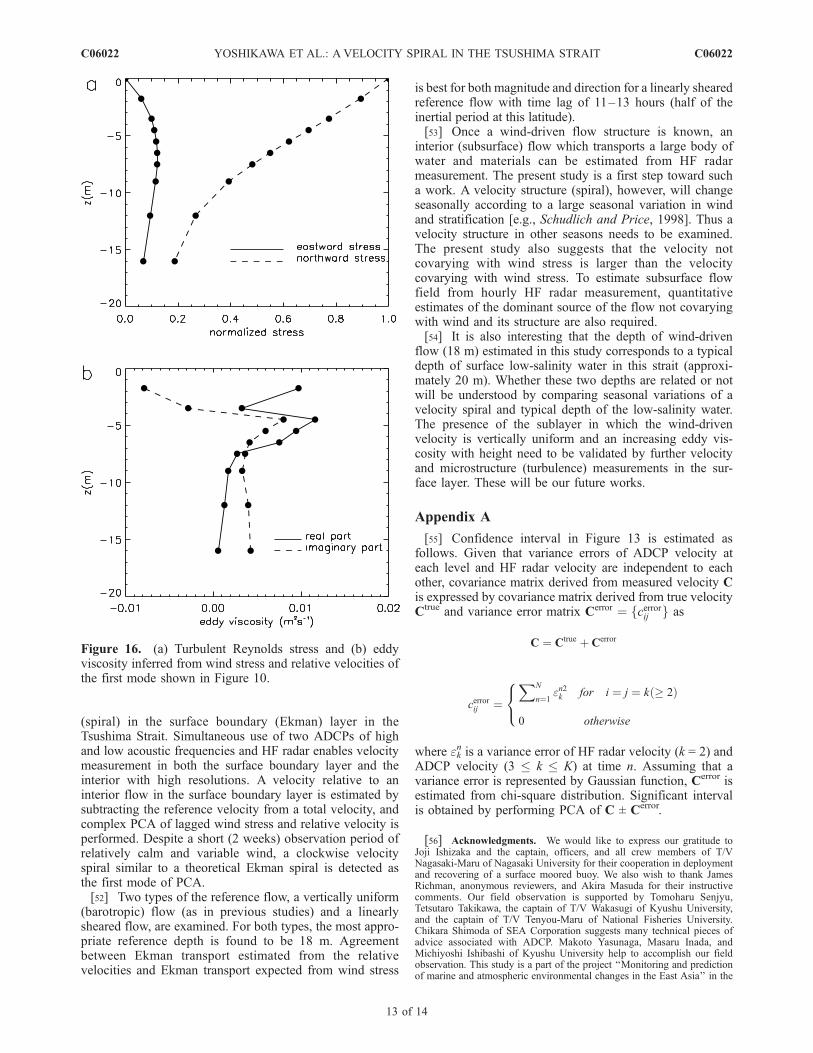
where r (=1020 kg m�3) is water density. Three-pointsmoothing in the vertical is first applied to u(z) and v(z), andthe first equation is integrated from the surface (whereturbulent stress is assumed equal to wind stress) to greaterdepth to give tx(z) and ty(z). Vertical eddy viscosity is thendiagnosed from the second equation. Although eddy viscosityestimated in this way can be a complex number, only its realpart has a physical meaning. The imaginary part can beinterpreted as a measure of the invalidity of Ekman balance.[48] Figure 16 shows vertical profiles of turbulent stress

and eddy viscosity. Turbulent stress is largest at the surfaceand smoothly reduces in magnitude at greater depth as

expected from Ekman theory. The real part of eddy viscosityis also largest (1.2 � 10�2 m2 s�1) near the surface andbecomes smaller (7.3 � 10�4 m2 s�1) at greater depth. Aprofile of eddy viscosity is less smooth than that of turbulentstress since the former is calculated from a derivative of therelative velocity (and hence is likely to be contaminated bynoise) while the latter is estimated from its integration.Magnitude of eddy viscosity corresponds to Ekman depth(2m/f )1/2 of 4.24–17.2 m, in which an e-folding depth scale(12.8 m) of the relative velocities of the first mode lies(Figure 11).[49] Inferred eddy viscosity increases with height up to

2.5 m depth where wave motion is dominant. Chereskin[1995] also inferred eddy viscosity deeper than 8 m depthfrom observed velocity spiral to find that eddy viscosity isgenerally larger at shallower depths. These results do notagree with the eddy viscosity model proposed by Madsen[1977], in which logarithmic boundary layer and decreasingeddy viscosity with height are assumed. The possible causeof increasing eddy viscosity with height will be wave-induced turbulence, which will be larger at shallowerdepths, although it cannot be confirmed in the present study.[50] A large imaginary part of eddy viscosity on the other

hand suggests invalidity of the above estimation. There willbe several reasons for this invalidity. One is bias errors ofADCP and HF radar velocities. Use of different devices thathave different measurement properties might affect theanomalously small estimation of eddy viscosity at 3.5 mdepth. Second is an assumption of constant eddy viscosity.Actual eddy viscosity is large when wind is strong, asexpected from time variation of thermal stratification(Figure 8). Thus, for further discussion of eddy viscosityprofile, it needs to be measured in a quantitative manner by,for example, a microstructure profiler.

7. Concluding Remarks

[51] Moored ADCP velocities and HF radar velocities for2 weeks are investigated to detect a velocity structure

Figure 14. Wind stress and relative velocities of thesecond mode. Color legends are same as in Figure 9. Windstress is set to point to the south.

Figure 15. Magnitude of the second mode score (blackline). Gray line shows an intensity of higher-order velocityshear of an interior flow ((gu + gv)/2).


12 of 14

C06022

(spiral) in the surface boundary (Ekman) layer in theTsushima Strait. Simultaneous use of two ADCPs of highand low acoustic frequencies and HF radar enables velocitymeasurement in both the surface boundary layer and theinterior with high resolutions. A velocity relative to aninterior flow in the surface boundary layer is estimated bysubtracting the reference velocity from a total velocity, andcomplex PCA of lagged wind stress and relative velocity isperformed. Despite a short (2 weeks) observation period ofrelatively calm and variable wind, a clockwise velocityspiral similar to a theoretical Ekman spiral is detected asthe first mode of PCA.[52] Two types of the reference flow, a vertically uniform

(barotropic) flow (as in previous studies) and a linearlysheared flow, are examined. For both types, the most appro-priate reference depth is found to be 18 m. Agreementbetween Ekman transport estimated from the relativevelocities and Ekman transport expected from wind stress

is best for both magnitude and direction for a linearly shearedreference flow with time lag of 11–13 hours (half of theinertial period at this latitude).[53] Once a wind-driven flow structure is known, an

interior (subsurface) flow which transports a large body ofwater and materials can be estimated from HF radarmeasurement. The present study is a first step toward sucha work. A velocity structure (spiral), however, will changeseasonally according to a large seasonal variation in windand stratification [e.g., Schudlich and Price, 1998]. Thus avelocity structure in other seasons needs to be examined.The present study also suggests that the velocity notcovarying with wind stress is larger than the velocitycovarying with wind stress. To estimate subsurface flowfield from hourly HF radar measurement, quantitativeestimates of the dominant source of the flow not covaryingwith wind and its structure are also required.[54] It is also interesting that the depth of wind-driven

flow (18 m) estimated in this study corresponds to a typicaldepth of surface low-salinity water in this strait (approxi-mately 20 m). Whether these two depths are related or notwill be understood by comparing seasonal variations of avelocity spiral and typical depth of the low-salinity water.The presence of the sublayer in which the wind-drivenvelocity is vertically uniform and an increasing eddy vis-cosity with height need to be validated by further velocityand microstructure (turbulence) measurements in the sur-face layer. These will be our future works.

Appendix A

[55] Confidence interval in Figure 13 is estimated asfollows. Given that variance errors of ADCP velocity ateach level and HF radar velocity are independent to eachother, covariance matrix derived from measured velocity Cis expressed by covariance matrix derived from true velocityCtrue and variance error matrix Cerror ¼ fcerrorij g as

C ¼ Ctrue þ Cerror

cerrorij ¼

XN

n¼1en2k for i ¼ j ¼ kð 2Þ

0 otherwise

8<:

where ekn is a variance error of HF radar velocity (k = 2) and

ADCP velocity (3 � k � K) at time n. Assuming that avariance error is represented by Gaussian function, Cerror isestimated from chi-square distribution. Significant intervalis obtained by performing PCA of C ± Cerror.

[56] Acknowledgments. We would like to express our gratitude toJoji Ishizaka and the captain, officers, and all crew members of T/VNagasaki-Maru of Nagasaki University for their cooperation in deploymentand recovering of a surface moored buoy. We also wish to thank JamesRichman, anonymous reviewers, and Akira Masuda for their instructivecomments. Our field observation is supported by Tomoharu Senjyu,Tetsutaro Takikawa, the captain of T/V Wakasugi of Kyushu University,and the captain of T/V Tenyou-Maru of National Fisheries University.Chikara Shimoda of SEA Corporation suggests many technical pieces ofadvice associated with ADCP. Makoto Yasunaga, Masaru Inada, andMichiyoshi Ishibashi of Kyushu University help to accomplish our fieldobservation. This study is a part of the project ‘‘Monitoring and predictionof marine and atmospheric environmental changes in the East Asia’’ in the

Figure 16. (a) Turbulent Reynolds stress and (b) eddyviscosity inferred from wind stress and relative velocities ofthe first mode shown in Figure 10.


13 of 14

C06022

Research Institute for Applied Mechanics, Kyushu University. This studyis also supported in part by Grant-in-Aid for Scientific Research (B) ofthe Ministry of Education, Culture, Sports, Science and Technology(17340141).

ReferencesChereskin, T. K. (1995), Direct evidence for an Ekman balance in theCalifornia Current, J. Geophys. Res., 100(C9), 18,261–18,269.

Ekman, V. W. (1905), On the influence of the Earth’s rotation on oceancurrents, Ark. Mat. Astron. Fys., 2, 1–53.

Kundu, P. K., and J. S. Allen (1976), Some three-dimensional characteristicsof low-frequency current fluctuations near the Oregon coast, J. Phys.Oceanogr., 6, 181–199.

Lee, C. M., and C. C. Eriksen (1996), The subinertial momentum balanceof the North Atlantic subtropical convergence zone, J. Phys. Oceanogr.,26, 1690–1704.

Madsen, O. S. (1977), A realistic model of the wind-induced Ekmanboundary layer, J. Phys. Oceanogr., 7, 248–255.

Nadai, A., H. Kuroiwa, M. Mizutori, and S. Sakai (1999), Measurement ofocean surface currents by the CRL HF ocean surface radar of FMCWtype: Part 2. Current vector, J. Oceanogr. Soc. Jpn., 7, 248–255.

Price, J. F., R. A. Weller, and R. Pinkel (1986), Diurnal cycling: Observa-tions and models of the upper ocean response to diurnal heating, cooling,and wind mixing, J. Geophys. Res., 91(C7), 8411–8427.

Richman, J. G., R. A. DeSzoeke, and R. E. Davis (1987), Measurement ofnear-surface shear in the ocean, J. Geophys. Res., 92(C3), 2851–2858.

Schudlich, R. R., and J. F. Price (1998), Observation of seasonal variationin the Ekman layer, J. Phys. Oceanogr., 28, 1187–1204.

Stacey, M. W., S. Pond, and P. H. LeBlond (1986), A wind-forced Ekmanspiral as a good statistical fit to low-frequency currents in a coastal strait,Science, 223, 470–472.

Weller, R. A. (1981), Observations of the velocity response to wind forcingin the upper ocean, J. Geophys. Res., 86(C3), 1969–1977.

Weller, R. A., D. L. Rudnick, C. C. Eriksen, K. L. Polzin, N. S. Oakey, J. W.Toole, R. W. Schmitt, and R. T. Pollard (1991), Forced ocean responseduring the Frontal Air-Sea Interaction Experiment, J. Geophys. Res.,96(C5), 8611–8638.

Wijffels, S., E. Firing, and H. Bryden (1994), Direct observation of theEkman balance at 10�N in the Pacific, J. Phys. Oceanogr., 24, 1666–1679.

Yelland, M., and P. K. Taylor (1996), Wind stress measurement from theopen ocean, J. Phys. Oceanogr., 26, 541–558.

Yoshikawa, Y., A. Masuda, K. Marubayashi, M. Ishibashi, and A. Okuno(2006), On the accuracy of HF radar measurement in the Tsushima Strait,J. Geophys. Res., 111, C04009, doi:10.1029/2005JC003232.

��K. Fukudome, Interdisciplinary Graduate School of Engineering

Sciences, Kyushu University, Kasuga, Fukuoka, Japan.K. Marubayashi, T. Matsuno, and Y. Yoshikawa, Research Institute for

Applied Mechanics, Kyushu University, 6-1 Kasuga Park, Kasuga,Fukuoka 816-8580, Japan. ([email protected])


14 of 14

C06022

a surface velocity spiral observed with adcp and hf · pdf filea surface velocity spiral...

Documents