CRM D0004085.A2 / FinalNovember 2001

A Survey of Enlisted Retention:Models and Findings

Matthew S. Goldberg

CNA4825 Mark Center Drive • Alexandria, Virginia 22311-1850

Copyright CNA ~orporation/~canned October 2002

Approved for distribution: November 2001

This document represents the best opinion of CNA at the time of issue. It does not necessarily represent the opinion of the Department of the Navy.

Approved for Public Release; Distribution Un limited. Specific authority: N00014-00-D-0700. For copies of this document call: CNA Document Control and Distribution Section at 703-824-2123.

Copyright O 2001 The CNA Corporation

Contents

Introduction and summary . . . . . . . . . . . . . . . . . . . . . . . . . . . . . . . . . . . . . . . . . . . . . . . . . . . . . . . . . . . . . . . . . . 1

ACOL model . . . . . . . . . . . . . . . . . . . . . . . . . . . . . . . . . . . . . . . . . . . . . . . . . . . . . . . . . . . . . . . . . . . . . . . . . . . . . . . . . . . . . . . . 7ACOL time horizon .......................................................................9"Optimality" of the ACOL time horizon .....................................12Statistical estimation of the ACOL model ..................................15

Panelprobitmodels . . . . . . . . . . . . . . . . . . . . . . . . . . . . . . . . . . . . . . . . . . . . . . . . . . . . . . . . . . . . . . . . . . . . . . . . . . . 1 7ACOL-2 model ............................................................................18Dynamic-programming models ...................................................23

Conditional logit models . . . . . . . . . . . . . . . . . . . . . . . . . . . . . . . . . . . . . . . . . . . . . . . . . . . . . . . . . . . . . . . . . . . 2 7Logit models with correlated taste factors ..................................28Nested logit model .......................................................................30

Multinomial logit models . . . . . . . . . . . . . . . . . . . . . . . . . . . . . . . . . . . . . . . . . . . . . . . . . . . . . . . . . . . . . . . . . . . 3 3Interpretation of the multinomial logit model ..........................35Conclusions ..................................................................................37

Reverse causation between bonuses and the reenlistment rate . . . . . . 39Individual data ..............................................................................39Panel data .....................................................................................41

Joint models of attrition and retention . . . . . . . . . . . . . . . . . . . . . . . . . . . . . . . . . . . . . . . . . . . . . 4 3Binary attrition models ................................................................44Continuous-time models of attrition and reenlistment .............46

Elasticity computation . . . . . . . . . . . . . . . . . . . . . . . . . . . . . . . . . . . . . . . . . . . . . . . . . . . . . . . . . . . . . . . . . . . . . . . . 5 1Definition of reenlistment ...........................................................51Definition of military pay .............................................................52

Elasticity estimates . . . . . . . . . . . . . . . . . . . . . . . . . . . . . . . . . . . . . . . . . . . . . . . . . . . . . . . . . . . . . . . . . . . . . . . . . . . . . 5 7Pay elasticities ...............................................................................57SRB effects ....................................................................................61

Relative stability of SRB effects ....................................................63

Estimation of discount rates . . . . . . . . . . . . . . . . . . . . . . . . . . . . . . . . . . . . . . . . . . . . . . . . . . . . . . . . . . . . . . 6 7Other discount-rate estimates .....................................................69Warner and Fleeter study ............................................................70

Effects of variables other than pay . . . . . . . . . . . . . . . . . . . . . . . . . . . . . . . . . . . . . . . . . . . . . . . . . . . 7 7Personal characteristics ...............................................................77Sea duty ........................................................................................78Personnel tempo ..........................................................................78

Areas for future research . . . . . . . . . . . . . . . . . . . . . . . . . . . . . . . . . . . . . . . . . . . . . . . . . . . . . . . . . . . . . . . . . . 8 1

References . . . . . . . . . . . . . . . . . . . . . . . . . . . . . . . . . . . . . . . . . . . . . . . . . . . . . . . . . . . . . . . . . . . . . . . . . . . . . . . . . . . . . . . . . . 8 3

List of figures . . . . . . . . . . . . . . . . . . . . . . . . . . . . . . . . . . . . . . . . . . . . . . . . . . . . . . . . . . . . . . . . . . . . . . . . . . . . . . . . . . . . . 9 1

Distribution list . . . . . . . . . . . . . . . . . . . . . . . . . . . . . . . . . . . . . . . . . . . . . . . . . . . . . . . . . . . . . . . . . . . . . . . . . . . . . . . . . . 9 3

11

Introduction and summaryThe supply of manpower has always been a concern to the military,but this issue took on greater importance in the events leading up tothe creation of the All-Volunteer Force (AVF) in 1973. In 1969, Presi-dent Nixon established the President's Commission on an All-Volunteer Force, commonly known as the Gates Commission. Thecommission's staff papers were among the first to systematically studythe supply of both enlistments and reenlistments to the military.These papers, along with concurrent literature in the professionaleconomics journals, demonstrated that an AVF was feasible from afiscal perspective.1

A variety of studies through the early and mid-1970s continued to ex-amine the supply of reenlistments. A major advance occurred duringthe late 1970s with development of the Annualized-Cost-of-Leaving(ACOL) model. Under this model, the primary driver of the re-enlistment decision is the discounted difference between the militarypay stream from reenlisting, and the civilian pay stream from leavingthe military. In particular, ACOL combined all the elements of mili-tary pay (basic pay, allowances, reenlistment bonuses, retirement pay)into a single, discounted present value. Moreover, ACOL suggested atime horizon over which the military and civilian pay streams must bemeasured and compared. From a statistical perspective, ACOL ex-pressed the reenlistment rate as a logit or probit function of the dis-counted pay difference, and possibly other regressors.

The concurrent literature includes Altman and Fechter [1], Fisher [2],Hansen and Weisbrod [3], Miller [4], and Oi [5]. These papers alsomade the important distinction between the fiscal cost of an AVF and theopportunity cost of diverting individuals from the civilian careers theywould otherwise have pursued.

For example, see [6, 7, and 8].

In parallel to ACOL, Glenn Gotz and John McCall developed adynamic-programming model of Air Force officer retention [9, 10].Rather than specifying a single, dominant time horizon, their modelallowed for probabilistic weighting of multiple time horizons. Al-though their model was theoretically elegant, it proved difficult to es-timate given the computer hardware and software environment ofthe early 1980s.

ACOL remained the conventional point of departure for much of theresearch conducted during the 1980s and 1990s. However, consider-able effort went into improving the statistical estimation of reenlist-ment models. That research effort took two major directions. First,panel probit models were formulated to better track the compositionof cohorts making successive reenlistment decisions during theirmilitary careers. For example, those induced to reenlist by a SelectiveReenlistment Bonus (SRB) might have less of a taste for military lifethan others who would have reenlisted even absent an SRB. Thesebonus-induced individuals would be less likely to remain in the mili-tary at subsequent decision points, unless the SRB were sustained.Panel probit models are designed precisely to capture the effects ofcohort composition on the outcome of successive binary decisions.

The second research direction was to recognize the distinction be-tween reenlistments (i.e., commitments for 36 or more additionalmonths of service) and shorter extensions. Only individuals who re-enlist are eligible to receive SRBs. Thus, an increase in SRB levels notonly will increase the total retention rate but also will change the mixof individuals retained between those who reenlist and those whomerely extend. The resulting change in the mix of commitments isclearly important for personnel planning purposes. Thus, a binarylogit or probit model was replaced by a trichotomous model, such asconditional logit, multinomial logit, or nested logit.

The statistics literature tells us little about adding cohort-compositioneffects to trichotomous choice models. The panel probit approachand the various trichotomous logit approaches have advanced essen-tially independently, although some of the same researchers have ap-plied both approaches, at one time or another, in modeling thereenlistment decision.

Other statistical problems have prompted researchers to modify orenhance the logit or probit models in various ways. First, there maybe reverse causation between pay and the reenlistment rate. The goalof the analysis is to estimate the positive effects of SRB and other in-centives on the reenlistment rate. However, enlisted occupations withchronically low reenlistment rates tend to be compensated withhigher SRB levels. This pattern of reverse causation may lead to adownward bias in the estimated pay coefficient. At least two studies[11 and 12] have used panel data and applied a fixed-effect estimatorin an effort to alleviate this source of bias.

We have already discussed the possibility that people who reenlist foran SRB might be less likely to reenlist a second time. Similarly, thosewho enlist for an accession bonus might be less likely to reenlist atthe first-term decision point. Two studies [13 and 14] have attemptedto control for the composition of the accession cohort when model-ing the first-term reenlistment decision. They did so by jointly model-ing survival to the first-term decision point with the outcome of thatdecision.

Several issues arise in computing the elasticity of the reenlistmentrate with respect to military pay. The definition of "reenlistment" iscomplicated by a number of factors, including reenlistment eligibilityand the treatment of extensions. Some studies exclude individualsdeclared ineligible to reenlist from the denominator of the reenlist-ment rate. However, the eligibility determination may be endogenousif, for example, individuals expressing a disinclination to reenlist aresubsequently declared ineligible by their units. Some studies combineextensions with reenlistments, modeling total retention. Others defertheir analysis of extensions, instead tracking them to learn whetherthey ultimately reenlist. It is difficult to compare the pay elasticitiesfrom studies that differ in their treatment of extensions.

Computation of the pay elasticity is further complicated by the defini-tion of "military pay." Many studies measure pay in terms of ACOL orsome other difference between the military and civilian pay streams.However, it is perilous to direcdy compute the elasticity of the re-enlistment rate with respect to a pay difference. The elasticity, so com-puted, will have the same algebraic sign as the baseline paydifference. Thus, even if increased pay has a positive effect in

encouraging more reenlistments, the elasticity may be zero or evennegative. Instead, the model should be exercised by hypothesizing afixed, discrete increase in military pay (e.g., $1,000). Express this in-crease as a percentage of baseline military pay, and divide the result-ing percentage increase in the reenlistment rate by the percentageincrease in military pay. This procedure estimates the arc elasticitywith respect to military pay (not the pay difference), and is guaran-teed to yield the correct algebraic sign.

At various points in time, the SRB has been paid either as a lump-sumon the date of reenlistment, or in equal annual installments over theduration of the reenlistment contract (with no indexing for inflation).To the first order of approximation, lump-sum bonuses are cost-effective if military members' discount rates exceed that of the federalgovernment.3 Since 1992, the Office of Management and Budget(OMB) has tied the federal government's discount rate to the marketrate on Treasury bonds. Several studies have estimated the discountrates of military members. Two of these studies [12 and 15] exploitedthe natural experiment that occurred when the method of SRB pay-ment switched from annual installments to lump-sum payments. Theestimates of military members' real (i.e., inflation-adjusted) discountrates are in the range of 6 to 26 percent. By contrast, real Treasuryrates have generally been in the range of 3 to 4 percent. Thus, lump-sum bonuses are the preferred method of payment.

Finally, several studies have investigated the retention effects of vari-ables other than relative military pay. In studies specific to the Navy,the variables of interest have included the incidence of sea duty,length of deployment, time between deployments, and percentage oftime spent under way while not deployed [16, 17, and 18]. The Navystudies have also estimated the SRB and other incentives required tocompensate for adverse changes in these duty characteristics. A morerecent study has measured additional duty characteristics and ex-tended the analysis to all four military services [19].

a

Other considerations include progressive income taxation and govern-ment recoupment of lump-sum bonuses from individuals who separateduring the contract period. Empirically, these factors are minor and donot change the basic conclusion.

The remainder of this report reviews each of the aforementionedmethodological issues in detail. It also presents a summary of the payelasticities estimated using the various measurement and statisticaltechniques. Although we cannot rationalize all of the variation in payelasticities, we attempt to correlate the elasticities with the techniquesused to estimate them.

THIS PAGE INTENTIONALLY LEFT BLANK

ACOL modelJohn Warner and his various collaborators developed the ACOLmodel in a series of papers. The initial motivation was to study a pro-posal by the President's Commission on Military Compensation(PCMC) to reform the military retirement system [20]. Warner alsoprogrammed a forecasting version of the model in the APL language.He distributed the model to the Navy Bureau of Personnel (BuPers)and, later, to the Office of the Assistant Secretary of Defense (Man-power, Reserve Affairs, and Logistics). BuPers started using themodel to analyze manpower issues in the Navy's Program ObjectivesMemorandum (POM), beginning with POM 1982. By the early 1980s,the ACOL model was well known and accepted throughout the de-fense manpower community.

The ACOL model's first appearance in the academic literature was a1984 paper by three of its codevelopers, Enns, Nelson, and Warner[21]. During that same year, Warner and Goldberg [18] published anapplication of the ACOL model in a mainstream economics journal.Parallel developments were taking place in the literature on retire-ment from civilian-sector jobs (e.g., Stock and Wise [22], who wereapparently unaware of the ACOL model). The two strands in the lit-erature were eventually brought together by Lumsdaine, Stock, andWise [23] and Daula and Moffitt [24].

Economic theory suggests that individuals combine all the elementsof compensation associated with any alternative into a single meas-ure, typically the discounted present value. In our context, SRBs pro-vide both cross-section (i.e., across military occupations) and time-series variation in discounted pay. Civilian earnings provide time-series variation, and may provide additional cross-section variation tothe extent that the civilian earnings functions account for militaryoccupation. Military pay excluding SRBs (i.e., Regular Military Com-pensation, or RMC) provides time-series variation but only minimal

cross-section variation (to the extent that differences in promotionrates are captured).

If the three pay components (SRBs, civilian earnings, and RMC) wereentered as separate regressors, their respective coefficients would al-most certainly be different. RMC would probably have the least sig-nificant coefficient because RMC has the least sample variation.However, it would be wrong to conclude that increases in RMC havethe smallest impact on retention. To estimate the effect of RMC moreprecisely, one could divide RMC by civilian earnings, thereby formingan index of relative military pay. The coefficient on this index wouldbe driven largely by the variation in civilian earnings, but it could beused to forecast the effects of changes in RMC on retention. Theseforecasts would be valid as long as individuals were indifferent be-tween an increase in RMC and an equal percentage decrease in civil-ian earnings.

It is even more difficult to compare the efficacy of increases in RMCversus increases in SRBs. One difference is that SRBs can be targetedto military occupations experiencing retention problems. Anotherdifference is that SRBs have a different time dimension from RMC.SRBs represent one-time payments or, at most, a short series ofannual installments. On the contrary, a given dollar increase in RMCpersists for the duration of a person's military career. Thus, an in-crease in RMC cannot be evaluated without knowing (or at least es-timating) the person's time horizon. Moreover, for those whose timehorizons extend to 20 or more years of service, basic pay (the largestelement of RMC) also affects their retirement annuity. Table 1 com-pares the time dimensions of these various elements of pay.

The ACOL approach solves the dimensionality problem by combin-ing all the elements of compensation into a single measure. In par-ticular, the rich sample variation in SRBs can be brought to bear inestimating the coefficient on the ACOL variable in a logit or probitchoice model. The ACOL coefficient, in turn, can be used to forecastthe effects of any change in compensation, including changes in theretirement system. Indeed, the ACOL approach was developed pre-cisely to study the military retirement system. We will also argue, in alater section, that the ACOL approach is consistent with the results of

studies that segmented compensation into multiple measures (e.g.,the SRB level and an index of relative military pay).

Table 1. Elements of pay and their time dimensions

______Ray element____________Time dimensions_______RMC (basic pay + allowances Persists over entire military career

+ tax advantage)

Basic pay Persists over entire military careerDetermines retirement annuity

SRBs Lump-sum is instantaneousAnnual installments over the

reenlistment contract

Civilian earnings stream Entire working life

ACOL time horizonThe ACOL approach suggests a time horizon for comparing the mili-tary and civilian discounted pay streams. However, construction of theACOL variable requires an assumption on military members' discountrates. We will describe methods for estimating discount rates in a latersection. For now, we merely report that enlisted personnel at their first-term and second-term reenlistment points appear to have real (i.e., netof inflation) discount rates of 6 to 26 percent.

To develop the ACOL variable, suppose initially that the retentiondecision were made solely by comparing the military and civilian dis-counted pay streams. Then, assuming that the pay streams could bemeasured precisely, we could predict with certainty the choice made byany individual—simply the one yielding the highest discounted paystream.

Relaxing these assumptions gradually, suppose next that the paystreams were known exactly to the individual decision-maker, but notto the data analyst. This would be the case if the analyst were using a

regression function to predict civilian earnings, yet the individual hadmore precise knowledge of his or her own earnings potential. In thissituation, we could no longer predict an individual's choice with cer-tainty. Instead, we could predict only the probabilities of staying orleaving for each individual.

As a further relaxation, we can recognize that a person's occupationalchoice depends on a comparison not only of discounted pay streamsbut also of the nonmonetary advantages and disadvantages of militaryversus civilian life. A general assumption in the literature is that thenonmonetary factors may be expressed as monetary equivalents (e.g.,"I will remain in the military only if they pay me $1,000 more per yearthan I could earn as a civilian"). Most authors further combine thenonmonetary factors with the unmeasured portion of the paystreams, and label the result the "taste factor." Continuing the exam-ple, suppose that the same person who requires a $1,000 annualpremium also knows that his or her potential civilian earnings are$500 above the regression prediction. The taste factor for this personwould be the sum, $1,500. Note also that the taste factor could benegative if people prefer military life or if their potential civilianearnings are below the regression prediction.

Suppose, for the moment, that a person currently in year of service(YOS) t is contemplating only two choices: remain in the military foran additional s years, or leave immediately. He or she will remain inthe military if:

) ' -- , (1);=/+! ;'=;+!

where M. is military pay (including any SRBs) in YOS j, C. is potentialcivilian pay in the same year, and v is the taste factor. Note that the

10

taste factor is assumed to be time-invariant.4 Equivalently, the personwill remain in the military if:

ACOLS ^ j=t+l t+s ————————— > v. (2)

As its name suggests, the ACOL variable is simply the annualized (orannuitized) difference between the military and civilian pay streams.Put differently, a stream of s pay differences, each equal to ACOLs,has the same discounted value as the pay stream{(M j — Cj), j = t + 1,...,? + s} , namely, the numerator of the previousexpression for ACOLs

Now considering all possible horizons {s = 1,2,3,...} , the person willremain in the military if there is at least one horizon over whichACOL exceeds the taste factor. Mathemati cally, this condition isequivalent to having the maximum ACOL greater than the tastefactor:

Max^ACOLJ > v. (3)

Conversely, the individual will leave the military immediately if thereis no horizon over which ACOL exceeds the taste factor. Mathemati-cally, this condition is equivalent to having the maximum ACOL lessthan the taste factor:

Max^ACOLJ < v. (4)

Inequality (1) is written so that potential civilian pay depends on calendaryear (equivalently, the person's age), but not on the length of his or hermilitary career (i.e., not upon the value of s). This assumption can be re-laxed, at the expense of some additional terms that measure the gain orloss in potential civilian pay from continued military service. The ACOLexpression under this relaxation is found in [11] or [23].

11

Thus, the maximum ACOL summarizes all of the information on paystreams necessary to predict a person's retention decision. Earningsfurther than s* years into the future (where s* is the horizon thatmaximizes ACOL) need not be considered. This result is impressivebecause earnings beyond s*, even when discounted, need not be neg-ligible numerically; yet the retention decision can be made withoutconsidering them.

"Optimally" of the ACOL time horizonThe horizon s* is sometimes called the "optimal horizon," but thisnomenclature is misleading. It seems to imply that, among all possi-ble horizons that involve remaining in the military at least one addi-tional year, the horizon s* is the most preferred. However, somesimple counterexamples disprove this conjecture.3

Suppose the only two possible career lengths involve staying for oneadditional year (s = 1) or two additional years (5=2) . Suppose furtherthat the military/civilian pay differences are $2,000 in the first yearand $1,000 in the second year. If the discount rate is 10 percent, theACOL values are ACOL, = $2,000 and ACOL2 = $1,524. The optimalhorizon over which ACOL is maximized is s = 1 year. Thus, the per-son will stay in the military for some duration if the taste factor is lessthan the maximum ACOL, or $2,000. Yet he or she would prefer tostay for two additional years, rather than just one, if the taste factor issufficiently small (or negative). Specifically, having already stayed forone additional year, the person would prefer to stay for the second

In one of many published examples of the misleading use of the term"optimal horizon," Gotz [25, p. 266] states that, "associated with [theACOL variable] is a known optimal future quitting date." Black, Moffitt,and Warner [26, p. 270] agree with Gotz on this point: "the ACOLmodel assumes that the individual picks a single optimal date of leavingsome time in the future." A rare correct statement is found in Mackin etal. [27, p. C-5]: "Note that the ACOL measure should be considered anindex describing the financial incentive to stay at least one more year.The horizon associated with the maximum ACOL is not necessarily the op-timal leaving point" [emphasis added].

12

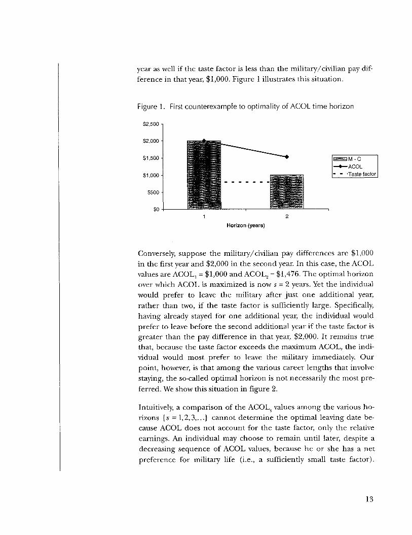
year as well if the taste factor is less than the military/civilian pay dif-ference in that year, $1,000. Figure 1 illustrates this situation.

Figure 1. First counterexample to optimality of ACOL time horizon

$2,500 n

Horizon (years)

Conversely, suppose the military/civilian pay differences are $1,000in the first year and $2,000 in the second year. In this case, the ACOLvalues are ACOL, = $1,000 and ACOL2 = $1,476. The optimal horizonover which ACOL is maximized is now s = 2 years. Yet the individualwould prefer to leave the military after just one additional year,rather than two, if the taste factor is sufficiently large. Specifically,having already stayed for one additional year, the individual wouldprefer to leave before the second additional year if the taste factor isgreater than the pay difference in that year, $2,000. It remains truethat, because the taste factor exceeds the maximum ACOL, the indi-vidual would most prefer to leave the military immediately. Ourpoint, however, is that among the various career lengths that involvestaying, the so-called optimal horizon is not necessarily the most pre-ferred. We show this situation in figure 2.

Intuitively, a comparison of the ACOLs values among the various ho-rizons {s = 1,2,3,...} cannot determine the optimal leaving date be-cause ACOL does not account for the taste factor, only the relativeearnings. An individual may choose to remain until later, despite adecreasing sequence of ACOL values, because he or she has a netpreference for military life (i.e., a sufficiently small taste factor).

13

Conversely, a person may choose to leave sooner despite an increas-ing sequence of ACOL values, because the taste factor is overwhelm-ingly large.

Figure 2. Second counterexample to optimality ofACOL time horizon

Horizon (years)

Daula and Moffitt [24] pointed out that, even if the taste factor isidentically zero, the optimal horizon that maximizes ACOL may dif-fer from the horizon that maximizes the discounted present value ofearnings. Returning to the first example, suppose that military earn-ings are $10,000 in both years. With the stated differentials, civilianearnings are $8,000 in the first year and $9,000 in the second year.The discounted present values (again using a 10-percent discountrate) are $16,182 for leaving immediately, $18,182 for staying oneadditional year and then leaving, and $19,091 for staying two addi-tional years. In this example, ACOL is maximized at s = I , yet the dis-counted present value of earnings is maximized at s = 2. With theassumed zero taste factor, the individual would prefer to stay for thesecond year in order to maximize discounted earnings. He or shewould be undeterred by the decline in ACOL values from ACOLj =$2,000 to ACOL2 = $1,524.

As a technical matter, the ACOL calculation truncates the militaryand civilian earnings streams after s years. However, the discountedpresent value of earnings is calculated through a predetermined

14

horizon—in practice, through an individual's entire working life, oreven longer if retirement pay is considered. Because it is truncated,ACOL is not a monotonic transformation of the discounted presentvalue over the predetermined horizon. Thus, the two expressionscould easily achieve their respective maxima at different values of 5.

None of these arguments vitiate the use of maximized ACOL to pre-dict the individual's retention decision (although we will soon con-sider some different arguments against the ACOL approach). But thearguments do militate against labeling as "optimal" the horizon overwhich ACOL is maximized.

Statistical estimation of the ACOL modelIf the distribution of the taste factor across decision-makers is nor-mal, the probability of staying in the military follows a probit model.If the distribution of the taste factor is logistic, the probability of stay-ing follows a logit model. Both of these models take the form ofS-curves, so that the estimated probability of staying increases up to alimit of 1.0 as conditions become more conducive to staying (e.g., asrelative military compensation increases). Conversely, the probabilityof staying decreases to a limit of 0.0 as conditions become less condu-cive to staying. When properly calibrated, the probit and logitS-curves are virtually indistinguishable, although the logit model issomewhat simpler mathematically and easier to compute. Software isreadily available to estimate both models.

The logit and probit models allow for the introduction of additionalregressors, apart from the maximum ACOL, that help explain the re-tention decision. For example, the retention rate has been found tovary directly with the civilian unemployment rate. The retention rateis also related to personal characteristics, such as marital status, race,education, and mental group.

The older studies estimated first-term and second-term retentionmodels completely independently of each other. Many studies usedgrouped data, but even studies that used individual (panel) datamade no allowance for correlation over time in the taste factor for agiven person. We will argue later that disregard for intertemporal

15

correlation likely led to upward-biased estimates of the coefficient onthe ACOL variable. As we will see, the ACOL-2 model imposes apermanent/transitory error structure in an effort to avoid this sourceof bias.

Independent of the ACOL developments, David Wise and his variouscollaborators developed an essentially equivalent model in their re-search on retirement from civilian-sector jobs. In particular, they in-dependently discovered the "maximum ACOL" condition (ourequation 3). Operationally, the only difference from ACOL is thatWise specified a first-order autocorrelation (AR1) error structurewhen estimating sequential retention decisions using panel data.

Interestingly, for a time Wise seemed unaware of the connection be-tween ACOL and his own research on civilian retirement. He was thediscussant on Warner and Solon's [14] paper at an Army retentionconference. Although the proceedings were published in 1991, theconference actually took place in 1989, at which time Wise must havebeen working on his paper with James Stock that would be publishedin 1990. Yet Wise [28, p. 278] made the following comment on War-ner and Solon, indicating his apparent lack of familiarity with theACOL concept:

the ACOL variable should be explained briefly in [Warnerand Solon's] paper. The authors refer the reader to expla-nations presented in other project reports. But the variableplays a key role in the analysis; several of the other variablesthat are included make little sense if the reader does notunderstand what the ACOL variable is supposed to capture.

The two strands in the literature were finally brought together byLumsdaine, Stock and Wise [23], some 3 years after the Army reten-tion conference; further developments were contained in Daula andMoffitt[24].

6 Stock and Wise [22], equations 2.12 through 2.14 on p. 1162;or Lumsdaine, Stock, and Wise [23], equation 10 on p. 27.

16

Panel probit modelsCritics of the ACOL approach point to its poor treatment of the dy-namics of retention over a person's military career. The ACOL valuesoften increase over one's career, as fewer years remain until retire-ment and the discounted value of the retirement annuity dramati-cally increases. According to a strict interpretation of the ACOLapproach, anyone who stayed at the first decision point would cer-tainly stay at all subsequent decision points because the taste factor isassumed time-invariant yet the financial incentive to stay (as meas-ured by the ACOL value) increases with time. As an empirical matter,however, we know that retention rates at the second and third deci-sion points are significantly below 1.0.

To develop a second criticism, consider a person who would have leftthe military after one term of service except for the lure of an SRB.This person has a larger taste factor (i.e., a larger distaste for militarylife) than others who would have stayed even absent an SRB. Unlessthe SRB is sustained, bonus-induced people are less likely to remainin the military at the second and subsequent decision points.

As an example, suppose the person had a taste factor of $2,000 and afirst-term baseline ACOL of $1,000, but was offered an SRB thatraised ACOL to $3,000. This person would stay through the first deci-sion point because ACOL ($3,000, including the SRB) exceeds thetaste factor ($2,000). However, the same individual would leave at thesecond decision point unless a sustained SRB or other compensationincentive raised ACOL above the baseline value of $1,000 to somevalue exceeding the (time-invariant) taste factor of $2,000. By con-trast, a non-bonus-induced person would stay at the second decisionpoint absent any compensation incentives. The latter individual, bydefinition, had a taste factor less than the baseline ACOL value of$1,000. This person would stay at the second decision point becausethe taste factor is time-invariant whereas ACOL tends, if anything, toincrease as retirement approaches.

17

We see that the second-term reenlistment rate depends on the cir-cumstances under which a person survived the first-term reenlistmentdecision. In an effort to capture this effect, Warner and Simon [29]included the lagged first-term ACOL value in a model to predict thesecond-term reenlistment rate. Along similar lines, Goldberg andWarner [30] include the lagged first-term SRB multiple in the sec-ond-term reenlistment model. The effect of lagged SRB was margin-ally significant with an unexpected positive sign for one occupationalgroup (Electronics), and highly significant with the expected nega-tive sign for one other occupational group (Non-electronics). Despitethe names of these two groups, they are not mutually exhaustive.Goldberg and Warner's taxonomy contained six other occupationalgroups, for which the lagged SRB effect was statistically insignificant.

ACOL-2 modelThe ACOL-2 model was an attempt to improve on ad hoc inclusionof lagged variables in second-term reenlistment models. Black, Ho-gan, and Sylwester [31] used the ACOL-2 model to predict retentiondecisions of Navy enlisted personnel. Black, Moffitt, and Warner [32]applied the model to retention decisions of Department of Defense(DoD) civilian employees. The ACOL-2 model was further devel-oped in a dialogue between the latter authors and Glenn Gotz [25],and in a subsequent paper on Army reenlistments by Daula andMoffitt [24].

The ACOL-2 model follows a long tradition in the literature onpanel data. Specifically, the taste factor for each person is decom-posed into (a) a permanent component, constant over time throughall decision points, and (b) a transitory component, randomly vary-ing over time from one decision point to another. This perma-nent/transitory structure has several advantages. First, the retentionrate is no longer predicted as 1.0 at the second and third decisionpoints. Returning to the example above, the person who stayed at thefirst decision point might choose to leave at the second decisionpoint, if the transitory component of the taste factor were sufficientlypositive. Several events, such as an unusually arduous tour of duty orfailure to receive an expected promotion, could "sour" a person at

18

the second decision point. This effect might offset the general ten-dency for ACOL to increase over the individual's career, causing himor her to leave the military at the second decision point.

Simply pooling retention data from several decision points, withoutimposing a permanent/transitory structure, would lead to an upward-biased estimate of the ACOL coefficient. We have noted both thegeneral tendency for ACOL to increase over an individual's career,and the general tendency for retention rates to increase (though notall the way to 1.0). Suppose that the first- and second-term data werepooled, but the two decisions for each person were treated as statisti-cally independent. Then the entire increase in retention rates wouldbe attributed to the increase in ACOL, leading to a large ACOL coef-ficient. In fact, however, part of the increase in retention rates resultsfrom the early departure from the sample of people with a strongerdistaste for the military. Put differently, the ACOL coefficient wouldpick up not only the effect of changes in relative compensation on afixed population, but also changes in the population composition it-self. This phenomenon, known as "unobserved heterogeneity," leadsto biased coefficient estimates.

Note that unobserved heterogeneity would not lead to any bias in theACOL coefficient estimated from a single cross-section of first-termreenlistment decisions. Nor would there be any bias if data werepooled on first-term reenlistment decisions made by different cohortsof individuals in consecutive fiscal years. Instead, the bias arises fromthe failure of the simple ACOL model to adequately track a cohort(or cohorts) of individuals through successive decision points. Thus,the bias would be manifest in simple ACOL models only when ap-plied at the second-term (or later) decision points.

The ACOL-2 model avoids the problem of unobserved heterogeneityby explicitly tracking the permanent taste distribution as a given co-hort advances through successive decision points. At each decisionpoint, the main forcing variable is again the maximum ACOL over allpossible horizons. Suppose, for example, that the first reenlistmentdecision occurs in 1990 after 4 years of service, and the second re-enlistment decision occurs in 1994 after 8 years of service. Then thefirst-term reenlistment decision is driven by the maximum ACOL

19

over the horizons of staying 1 additional year up to 26 additionalyears (assuming mandatory retirement after 30 years of service). Forthe second-term reenlistment decision, ACOL is recomputed overthe horizons of staying 1 additional year up to 22 additional years.Both ACOL values are computed using data from the fiscal years inwhich the respective decisions were made (e.g., a person's first-termdecision might be modeled using the military and civilian wages thatprevailed in 1990, but then the second-term decision would be mod-eled using the wages that prevailed in 1994). Thus, the model cap-tures not only a person's progression through a fixed military paytable but also any growth over time in the military pay table or in ci-vilian wages.7 The ACOL-2 model also allows additional regressors,such as the civilian unemployment rate. This variable, too, is meas-ured contemporaneously with the decision years, thus capturing ad-ditional information on trends in the civilian economy.

Black, Moffitt, and Warner [32] applied the ACOL-2 model to sepa-ration decisions of DoD civilian employees. Because estimation of theACOL-2 model requires numerical integration of the multivariatenormal density, they achieved a considerable computational effi-ciency by adopting a likelihood-factorization technique previouslydeveloped by Butler and Moffitt [33]. Glenn Gotz [25] wrote a com-ment on Black, Moffitt, and Warner, to which they immediately re-sponded. Some of Gotz's points apparently spurred Robert Moffittand his various collaborators to further improve on the ACOL-2formulation.

For example, in their study of Navy enlisted retention, Black, Hogan,and Sylwester [31] reported that the sample average ACOL value dou-bled (in constant dollars) from the first-term to the second-term decisionpoint. The average ACOL value nearly doubled again from the second-term to the third-term decision point.

20

In his comment, Gotz [25, p. 266] makes the following statement:

Recall that associated with [the ACOL variable] is a knownoptimal future quitting date [sic], t + 5*... .By construction of[Black, Moffitt and Warner's] model, any reduction in civilservice pay more than s* years from t [i.e., beyond the "op-timal future quitting date"] will have absolutely no effect onthe predicted quit rate at t.

Gotz's statement is too severe. When simulating a policy change,knowledgeable users of the ACOL model always recompute the se-quence of ACOL values and locate the new maximum ACOL value.Consider, for example, an increase in military retirement pay, andsuppose that the individual's horizon was initially 4 years ahead(t + 4). Gotz's statement implies that the horizon would remain fixedat t + 4 and, thus, the increase in retirement pay would have no effecton retention. In fact, the horizon might easily move out to year 20, sothat retirement pay now enters the calculation and affects retention.8

Figure 3 illustrates this situation for a first-term decision-maker. Inthe base case, ACOL is maximized over the horizon of a 4-year re-enlistment. The prospect of retirement pay after 20 years causes ajump in the ACOL value to nearly $4,500 at YOS 20, but that valuestill lies below the maximum ACOL of $5,000. Now consider an in-crease in the present value of retirement pay, equal to $100,000 whendiscounted to the date of retirement. The ACOL value jumps to al-most $7,000 at YOS 20, so the ACOL horizon now encompasses the20-year retirement point. The increase in the maximum ACOL from$5,000 to $7,000 provides a substantial retention incentive, eventhough the underlying change in compensation takes place beyondthe initial ACOL horizon.

Paradoxically, Gotz and his collaborators had already recognized thispoint 5 years earlier, although, like many others, they misinterpretedthe ACOL horizon as the planned leave point. According to Fernan-dez, Gotz, and Bell [34, p. 16]:

Indeed, recalculation of the ACOL horizon was included in the forecast-ing version of the ACOL model developed by John Warner in the early1980s.

21

the calculated ACOL for any particular decision point re-flects a specific horizon, the planned leave point [sic] forthe marginal individual. Changes in earnings beyond thathorizon generally do not affect the [maximum] ACOLvalue, and so cannot change the model's retention predic-tions for earlier decision points. Only an increase in militaryearnings (or decrease in potential civilian earnings) largeenough to move the horizon outward can have any effect.

Figure 3. Example of shift in ACOL time horizon

7,000 -i

6,000

Base caseS100K retirement increase

10 12 14Horizon endpoint (YDS)

16 18 20

It was clearly the intention of Black, Moffitt, and Warner [32, pp.258-259] that the maximum ACOL be recalculated after a policychange:

To incorporate [the effects of a policy change] a new set of[ACOL] values must be calculated and a [maximum] se-lected for each individual in the file. The recalculated[maximum ACOL] is then inserted into the quit model,along with the other variables and their respective parame-ters, to obtain a simulated pattern of quit rates.

Other authors, such as Daula and Moffitt [24, p. 520], recognized theneed to recalculate the maximum ACOL after a policy change,though again mislabeling the ACOL horizon as "optimal":

To construct the...ACOL forecasts...would require recalcu-lating optimal leaving dates [sic] at every date in the future(each of which requires rechecking all possible future leav-ing dates at each future date).

22

Dynamic-programming modelsAlong with John McCall, Glenn Gotz had developed a dynamic-programming model of Air Force officer retention [9, 10]. Their ap-proach was particularly well suited to modeling officer retention be-cause it offered the individual an opportunity to leave the militaryduring every future year. Although military officers certainly faceminimum service requirements, their mid-career commitments areusually less rigid than the typical 4-year terms served by enlisted per-sonnel. Gotz and McCall were also very careful in modeling alterna-tive promotion paths, capturing the adverse retention effect of beingpassed over for promotion.

Unfortunately, Gotz and McCall's formulation was computationallyintensive, especially given the computer hardware and softwareenvironment of the early 1980s. They were able to estimate only threemodel parameters: the mean and standard deviation of the perma-nent taste factor, and the standard deviation of the transitory tastefactor (the latter factor has a mean of zero by assumption). In par-ticular, they did not estimate the effects of other regressors, such asthe unemployment rate or various personal characteristics. Nor didthey estimate the discount rate, which they fixed a priori. Finally, theywere unable to estimate the standard errors of the three modelparameters.9

Moffitt and his collaborators took some lessons from Gotz and wenton to develop a dynamic-programming model of their own. Theirapproach was crystallized in an impressive paper by Daula and Moffitt[24]. Recall that the simple ACOL model summarizes the militaryand civilian pay streams with a single discounting calculation over the

A simple approximation was developed by Warner [35, pp. 27-28], whofit the three model parameters to the cross-sectional survival profile (byterm of service) that prevailed in the Navy enlisted force in FY 1979. Us-ing a grid search, Warner estimated the mean permanent taste factor as$2,800 (in FY 1979 dollars), the standard deviation of the permanenttaste factor as $3,500, and the standard deviation of the transitory tastefactor as $4,500. However, Warner reported that his objective functionwas extremely flat, so that many alternative sets of parameter values fitthe data about equally as well.

23

dominant optimal horizon. The ACOL-2 model tracks individualsthrough time, using contemporaneous pay streams to update theACOL calculation at each decision point. Thus, under ACOL-2 thereis a single, dominant horizon at the first-term decision point; a single(generally different) dominant horizon at the second-term decisionpoint; and so on. These calculations are illustrated in figure 4, wherethe dominant horizon shifts from YOS 7 when evaluated at the first-term decision point to YOS 20 when reevaluated at the second-termdecision point.

Figure 4. Example of recalculation of dominant time horizon

Evaluated at YOS 4Evaluated at YOS 8

10 12 14Horizon endpoint (YOS)

16 18 20

By contrast, at any particular decision point, Daula and Moffitt prob-abilistically weight the discounted pay differences over all future leav-ing points. Thus, there is no longer a single, dominant horizon.10 Inaddition, Daula and Moffitt were more careful in their specificationof the error terms than had been Black, Moffitt, and Warner [32].Finally, they estimated their model by embedding the dynamic pro-gram inside the panel probit approach of Butler and Moffitt [33].

The equivalence between dynamic programming and probabilisticweighting in this context had previously been established by Warner[35]. Further theoretical developments along these lines are found inHotz and Miller [36].

24

Daula and Moffitt [24] touted the ease with which their estimateswere computed: "we show that dynamic retention models are consid-erably less difficult to estimate than [the] literature implies" (p. 500);"estimation of the model in this form is not difficult...no difficultcalculations are involved" (p. 503); and "since the single-periodmodel is not overly burdensome itself, its multiple evaluation [usingpanel data] is still well within the power of modern computationalfacilities" (p. 507). However, they later conceded that estimation tookabout 450 CPU minutes per iteration, and six or seven iterations permodel run (p. 514). Thus, each model run took about 48 hours—hardly an improvement over Gotz and McCall.

For comparison purposes, Daula and Moffitt also estimated theACOL-2 model using the bivariate probit technique.11 Interestingly,they report that the log-likelihood value is slightly better for theACOL-2 model than for their dynamic-programming model. In lightof the computational difficulty of the latter (notwithstanding the au-thors' statements to the contrary), the ACOL-2 model becomes anextremely compelling alternative.

As Daula and Moffitt correctly point out, multivariate probit is equivalentto Butler and Moffitt's panel probit technique. The latter was developedprimarily for long panels spanning three or more decision points, toavoid numerical integration of the trivariate (or higher order) normaldensity. These days, both techniques are available in the LIMDEP pack-age developed by Econometric Software, Inc. (www.limdep.com). In fact,LIMDEP is advertised as being able to estimate the multivariate probitmodel with up to 20 correlated decisions, though one must be skepticalabout the computational speed of such high-dimensional models. Also, itshould be possible to program the panel probit model in PROGNLMIXEDofSAS.

25

THIS PAGE INTENTIONALLY LEFT BLANK

Conditional logit modelsMore detailed models partition the event "staying" into reenlistmentsand extensions. Reenlistments are defined as commitments to stay inthe military for 36 months or longer, whereas extensions are definedas commitments to stay for fewer than 36 months. The distinction be-tween reenlistments and extensions is clearly important for personnelplanning purposes. There are also behavioral differences, becauseonly those who reenlist are eligible to receive SRBs. We would expectan increase in the SRB level to increase the total probability of stay-ing. Underlying that effect, we would expect an increase in the SRBlevel to reduce the probability of extending but to increase the prob-ability of reenlisting by a larger magnitude.

Various models are available to estimate the three probabilities of re-enlisting, extending, or leaving. One approach, the conditional logitmodel, was pursued by Goldberg and Warner [30] and Goldberg[11]. These authors collected data on reenlistment, extension, andseparation rates in cells defined by fiscal year, Navy enlisted rating,and years of service (in the range of 3 to 6 years). They computed adiscounted pay stream associated with each of the three choices forthe "typical" sailor in each cell. In particular, the pay stream associ-ated with reenlistment contained the SRB, whereas the pay stream as-sociated with extension did not. Their models contained backgroundvariables, including the civilian unemployment rate, marital status(i.e., percentage married in each cell), race, education, and mentalgroup. They estimated coefficients from which one can compute themarginal effect of each background variable on the three choiceprobabilities.

Goldberg and Warner also estimated a single pay coefficient, inter-pretable as the "marginal utility of income." Using this coefficient, onecan compute the reallocation of the three choice probabilities in re-sponse to a change in the discounted pay stream associated with oneor more of the three choices. For example, a change in the SRB level

27

affects only the pay stream associated with reenlistment (which we de-note as M), but affects all three choice probabilities as follows:

(5)

dPJdM = -bPL PR,

where b is the pay coefficient and PR, Pe and Pl are the respectiveprobabilities of reenlisting, extending, and leaving.

Hogan and Black [37, p. 41] opine that,

The conditional logit model... is a poor choice in the analy-sis of extensions versus reenlistrnents because it constrainsreenlistment bonuses to reduce extensions by the same per-centage that it reduces losses.

Their statement of this mathematical property of the conditionallogit model is correct; in terms of percentage changes:

(cPE /dM)/ PE = -bPR = (dPL /dM)/ PL. (6)

Hogan and Black argue that reenlisting and extending are closersubstitutes than are reenlisting and leaving. If that were the case, anincrease in the SRB level would draw more reenlistrnents from thosewho otherwise would have extended, rather than from those whootherwise would have left. Thus, one might prefer an alternativemodel with the following mathematical property:

(dPE/dM}/PE<(dPL/dM)/PL < 0. (7)

Logit models with correlated taste factorsAlternative models, satisfying the Hogan and Black critique, may beformulated by returning to the theoretical underpinnings of occupa-tional choice. For this purpose, we change the notation slightly sothat each choice has its own taste factor. Thus, VR is the monetaryequivalent of the nonmonetary factors associated with reenlisting; VK

28

and VL are defined similarly for extending and leaving. The single"taste factor" in the earlier discussion would be interpreted asv= VL— VR, the net preference for civilian life.

McFadden [38] showed that the conditional logit model arises whenthe taste factors are independent across choices, each with an ex-treme-value distribution. It is not as well appreciated that the condi-tional logit model also arises when the taste factors have Gumbel'smultivariate logistic distribution, with correlations of 0.5 betweeneach pair of taste factors. " In either case, Hogan and Black's critiquecomes into greater focus. Suppose that reenlisting and extending areindeed closer substitutes than either of the other two pairs of choices.If so, the correlation between the taste factors for reenlisting and ex-tending should be larger than for the other two pairs of choices. Forexample, because reenlisting and extending are more similar, an in-dividual who requires an above-average premium for reenlistingrather than leaving should also require an above-average premiumfor extending rather than leaving. In other words, the taste factorsfor these two choices should have a particularly high correlation.However, the conditional logit model implicitly assumes equal corre-lations between all three pairs of choices.13

12 This result is due to Goldberg [11, pp. 80-81]; Gumbel's multivariate lo-gistic distribution is described in Johnson and Kotz [39, pp. 291-293].The oft-cited converse to McFadden's theorem states that, if the taste fac-tors are independent and the choice probabilities are of the logit form,then the taste factors are extreme-value distributed. However, the latterresult does not rule out correlated taste factors.

Another expression of the difficulty with the conditional logit model isthe "independence of irrelevant alternatives." In our example, the rela-tive probability of extending versus leaving depends on only the back-ground variables and the discounted pay streams associated with thesetwo choices. The relative probability does not depend on the pay streamassociated with reenlisting. In particular, it does not depend on the SRBlevel. Yet a person who extends could subsequently choose to reenlistand thereby receive an SRB. Thus, for many, the SRB level is an impor-tant determinant of the decision to extend versus leave.

29

Nested logit modelMcFadden's [40, 41] nested logit model allows for unequal correla-tions. Under this model, the taste factors associated with reenlistingand extending have a bivariate extreme-value distribution, with a cor-relation coefficient that is free to vary in the range of 0 to +1. Thetaste factor associated with leaving has a univariate extreme-value dis-tribution and is independent of the other two taste factors. In thespecial case where the correlation coefficient equals zero, the threetaste factors are all independent extreme-value distributed, and theconditional logit model results. If the correlation coefficient is posi-tive, however, the probability equations differ from those of the con-ditional logit model. In particular, the probability equations containthe correlation coefficient as a free parameter.

During the mid-1980s, Goldberg and Warner attempted to apply thenested logit model to grouped data on first-term reenlistment deci-sions in the Navy. Goldberg and Warner never published their resultsbecause they could not achieve convergence to reasonable parameterestimates. Nor could Mackin et al. [27] using microdata on individualNavy sailors.

Even when using microdata, there are two approaches to estimatingthe nested logit model. The first proceeds in two stages: (1) a logitmodel is estimated among individuals who stay, to predict probabilityof reenlisting versus extending, and (2) another logit model is esti-mated to predict the probability of staying (i.e., either reenlisting orextending) versus leaving. However, the second stage is not a stan-dard logit model. Instead, it contains an additional variable, known asthe "inclusive value," that must be constructed based on the results ofthe first stage. To avoid model failure due to multicollinearity, the in-clusive value must be computed from at least some variables that areabsent from the second-stage (stay/leave) model. That is, there mustbe some variables that drive the reenlist/extend decision but not thestay/leave decision. Mackin et al. opine that, because individual

30

decision-makers ultimately compare all three choices simultaneously,the required identifying variables simply do not exist.14

The second approach to estimating the nested logit model is full-information maximum-likelihood. This approach has only recentlybecome available using commercial software.= It would be interestingto apply this approach to the retention decision, to determinewhether it circumvents the problem of multicollinearity.

Another expedient was attempted by Warner [42], using groupeddata on first-term and second-term reenlistment decisions in the Ma-rine Corps. Warner estimated sequential logit models, but simplyomitted the inclusive value from the second-stage model. These se-quential logit models had good explanatory power and producedreasonable estimates of the pay elasticities. However, it is not knownwhat joint distribution of the taste factors, if any, would yield the se-quential logit probability equations (without the inclusive value).Thus, Warner's approach, though pragmatic, does not have strongtheoretical underpinnings.

Theoretically, the nested logit model is identified because the inclusivevalue is a nonlinear construct, thus not perfectly predictable from any lin-ear combination of second-stage regressors. As a practical matter, however,the degree of nonlinearity may not be adequate to identify the model.

LIMDEP version 7.0 includes this feature in the module NLOGITversion 2.0.

31

THIS PAGE INTENTIONALLY LEFT BLANK

Multinomial logit modelsRecall that Goldberg and Warner [30] and Goldberg [11] computeda discounted pay stream associated with each of the three choices,and estimated a single pay coefficient interpretable as the "marginalutility of income." Thus, their models contain terms of the form b MR,b Mp and b M[} where MR, Me and M[ are the respective pay streams.An alternative approach is to enter the pay variables in the samemanner as the background variables. Recall that a background vari-able, such as the unemployment rate, affects the probabilities of allthree choices. Three separate coefficients are estimated, from whichone can compute the effect of a change in the unemployment rateon each choice probability. Similarly, one could enter a pay variable,such as the SRB multiple or dollar amount, as a background variable,and compute its effect on each choice probability. Thus, the alterna-tive model would contain terms of the form ^SRB, bt SRB, andb, SRB.

In the econometrics literature, logit models in which the coefficientsare fixed across choices, but the regressors vary, are known as "condi-tional logit models." By contrast, logit models in which the regressorsare fixed across choices, but the coefficients vary, are known as"multinomial logit models."16

The multinomial logit model satisfies the Hogan and Black [37] cri-tique and breaks the "independence of irrelevant alternatives." Underthe multinomial logit model, the relative probability of extending ver-sus leaving is sensitive to the pay stream associated with reenlisting,

The term "conditional logit model" is unfortunate because it is not clear,in any statistical sense, which variable is conditional on which other vari-able. Nor is it clear why one model is "conditional" and the other (mul-tinomial) model is, presumably, "unconditional." More recently, Greene[43] has suggested the terminology "discrete choice model" to replace"conditional logit model."

33

particularly the SRB level. The extension and separation rates changeby (possibly) different percentages in response to an SRB increase:

- (dPL/dSKB)/PL = bE-bL (8)

This difference is precisely the coefficient on SRB in an extend/leavelog-odds model, and is a free parameter that may be of either alge-braic sign (not necessarily zero).

Hosek and Peterson [12] and Lakhani and Gilroy [44] estimatedmultinomial logit models. Reference [12, appendix B] reports nega-tive coefficients on the SRB level in extend/leave log-odds models, atboth the first-term and second-term decision points. These results in-dicate that Pp/Pj declines with increases in the SRB level, so that in-creased bonuses draw more reenlistments from those who otherwisewould have extended than from those who otherwise would have left.

Figure 5 shows the difference between the conditional and multino-mial logit models. Under the conditional logit model, a hypotheticalSRB increase causes the probabilities of extending and leaving toboth decrease by 20 percent. Under the multinomial logit model,more reenlistments are drawn from those who would have extended,so the extension probability decreases even more severely but theseparation probability decreases less severely.

Figure 5. Reallocation of probabilities when SRB level increases

Base probabilities

Conditional logit

Multinomial logit

I \ 50%

20% drop in both probabilities

greater percentage drop in extensions

60%

0% 10% 20% 30% 40% 50% 60% 70% 80% 90% 100%

Probabilities

34

Hogan [45] cautions that the pay coefficients bR, bp and b; in themultinomial logit model are not the same as the partial effects and,further, may even differ in sign from the partial effects. For example,the partial effect of the SRB level on the reenlistment rate is given by:

BPR/dSm=(bR-bI)PR(l-PR) - (bF-bL)PEPR,

= PR(bR(l-PR) -bEPE-bLPJ. (9)

This expression will differ in sign from bR if bR, bB and bl all have thesame sign, but bR has the smallest magnitude and PR is close to 1.0.Moreover, the standard error of dPR/dSRB is not immediately avail-able from those of bR, bp and br but can be derived from the underly-ing variances and covariances.

Interpretation of the multinomial logit modelAlthough the multinomial logit model breaks the "independence of ir-relevant alternatives," it leads to other problems of interpretation. Weargued earlier in favor of the ACOL approach, which combines all theelements of compensation into a single measure. The multinomiallogit models, as estimated by Hosek and Peterson [12] and Lakhaniand Gilroy [44], do not use a single measure of compensation. Instead,they segment compensation into two measures: the SRB level and anindex of relative military pay.

Lakhani and Gilroy seem to believe that, if the ACOL approach werecorrect, segmenting compensation into multiple measures shouldproduce equal elasticities on all of the measures. Conversely, if theelasticities prove unequal, the compensation measures should remaindistinct rather than being combined into a single ACOL variable.

Lakhani and Gilroy report that the SRB elasticities across Army occu-pations are, if anything, negatively correlated with the relative-payelasticities. They interpret this finding as evidence against the ACOLapproach, concluding [44, p. 241]:

The formula is given in Hosek and Peterson [12, appendix C].

35

It is, therefore, somewhat presumptuous to assume that theeffect of SRB is the same as that of relative pay, as is oftendone in the existing literature: Their dollar values are addedto retirement to represent the cost of leaving in the Annual-ized Cost of Leaving (ACOL) model.

We will now argue that, based on economic theory, there is no reasonto expect a positive correlation between the SRB and relative-payelasticities. Further, we will argue that the ACOL approach can ra-tionalize the observed negative correlation if there is, in turn, a posi-tive correlation between SRB levels and civilian earningsopportunities. This will be the case if military occupations with supe-rior civilian alternatives have chronically poor retention, and if SRBsare used to combat these retention problems. Thus, the observednegative correlation between the two elasticities, rather than being aparadox that vitiates the ACOL approach, is actually quite consistentwith that approach.

To simplify the algebra, suppose that the difference between militarypay (RMC) and civilian pay is constant over the individual's planninghorizon. We denote the annual difference as (M-C). The ACOL vari-able equals this quantity plus the annualized bonus. Again, to simplifythe algebra, assume a lump-sum SRB. The annualized value of theSRB, over an s-year horizon, is given by:

S R B ( l + r)" ;=SRB/Z). (10)/ ;=i

Thus, ACOL is given by:

ACOL = (M-C)+ SRB / D. (11)

18 For example, consider a lump-sum bonus, a 4—year planning horizon,and a 10-percent discount rate. Under these assumptions, the annualizedbonus evaluates at 0.315 x SRB. If this amount were paid at the end ofeach year over the 4-year planning horizon, the undiscounted total pay-ment would be 1.26 X SRB, but the discounted total payment would be ex-actly 1.00 x SRB.

36

Conclusions

Suppose we have an estimate of the elasticity of the retention prob-ability (P) with respect to ACOL:

E = (ACOL / P) (dP / 9ACOL) . (12)

We can derive the elasticity of the retention probability with respectto the military/ civilian pay difference:

] [dP/d(M-Q]

= [(M-C)/P] [dP/dACOL] [9ACOL / d(M- Q]

= £x (M-Q/ACOL; (13)

and with respect to the SRB amount:

[SRB/P] [3P/aSRB]

= [SRB / P] [dP/ 3ACOL] [9ACOL / 3SRB]

= (Ex SRB) / (Dx ACOL). (14)

Because all of the other terms are common, the correlation (acrossoccupations) between the latter two elasticities is essentially the cor-relation between (M - C) and SRB. Thus, the ACOL framework isconsistent with a negative correlation if SRBs are employed to com-pensate for salary shortfalls in selected military occupations.

We conclude that both the conditional logit model and the multino-mial logit model have considerable merit. The former is more firmlygrounded in economic theory, combining all the elements of com-pensation into a single measure of discounted pay. A wealth-maximizing individual would make his or her reenlistment decisionbased on this single measure, and no information is added by parti-tioning it into multiple components. Moreover, the rich sample varia-tion in SRBs can be brought to bear in estimating the single paycoefficient.

On the other hand, the conditional logit model suffers from the in-dependence of irrelevant alternatives. The multinomial logit modelrelaxes this restrictive assumption. However, as just demonstrated, the

37

elasticities on the multiple pay components must be interpreted withcaution. Moreover, some of the elasticities maybe underestimated forlack of sample variation (e.g., the index of relative military pay).

We agree with Hogan [45, p. 258], who states:

In the trichotomous logit model specified by Lakhani andGilroy, both the 8KB and relative wage variables are identi-cal across choices, while the coefficients on the variablesvary across the alternatives. Hosek and Peterson (1985) alsospecified the logit model in this way, whereas Goldberg(1984) constrained the coefficients to be the same and var-ied the level of the independent variable across choices. It isnot clear to me which specification is preferable.

Finally, we will see later (in table 2) that the pay effects estimatedfrom the two models are quite similar. Thus, a stark choice betweenthe two models is not entirely necessary.

38

Reverse causation between bonuses and thereenlistment rate

Goldberg [11] and Hosek and Peterson [12] were concerned aboutreverse causation in the relationship between pay and the reenlist-ment rate. The goal of the analysis is to estimate the positive effect ofpay, particularly reenlistment bonuses, in encouraging reenlistments.However, some enlisted occupations have suffered chronically poorretention because of arduous duty (e.g., Navy ratings with a high per-centage of time at sea), slow promotions, or lucrative civilian oppor-tunities. The enlisted occupations with chronically poor retention aregenerally awarded higher SRB levels. This pattern of reverse causa-tion leads to a downward bias in the estimated effect of pay on thereenlistment rate.

Individual dataIt is commonly believed that individual decision-makers are "price-takers" in the sense that, while their decisions may well be affected bySRB levels, their decisions do not, in turn, affect SRB levels. However,even individual data may be plagued by reverse causation that leadsto biased estimation of the bonus effect.

Figure 6 illustrates the situation. We have drawn the supply and de-mand curves for reenlistments, both as a function of the SRB level.We have drawn the demand curve as a vertical line, to capture rigidpersonnel requirements that are insensitive to the price level. How-ever, the analysis is virtually identical even if the demand curve exhib-its some elasticity.

The military service attempts to set SRB levels to equate the supply ofreenlistments to the desired level of demand. If the service errs on theside of too low an SRB level (e.g., SRB,), too few people reenlist(pointA), and a shortfall occurs (the distance AB). To alleviate the

39

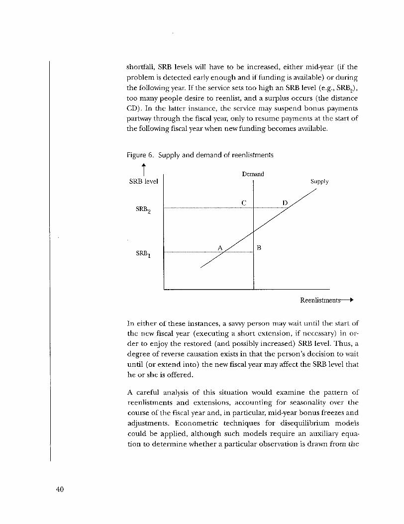
shortfall, SRB levels will have to be increased, either mid-year (if theproblem is detected early enough and if funding is available) or duringthe following year. If the service sets too high an SRB level (e.g., SRB2),too many people desire to reenlist, and a surplus occurs (the distanceCD). In the latter instance, the service may suspend bonus paymentspartway through the fiscal year, only to resume payments at the start ofthe following fiscal year when new funding becomes available.

Figure 6. Supply and demand of reenlistments

TSRB level

SRBo

SRB,

Demand

C

Supply

D

B

Reenlistments——>

In either of these instances, a savvy person may wait until the start ofthe new fiscal year (executing a short extension, if necessary) in or-der to enjoy the restored (and possibly increased) SRB level. Thus, adegree of reverse causation exists in that the person's decision to waituntil (or extend into) the new fiscal year may affect the SRB level thathe or she is offered.

A careful analysis of this situation would examine the pattern ofreenlistments and extensions, accounting for seasonality over thecourse of the fiscal year and, in particular, mid-year bonus freezes andadjustments. Econometric techniques for disequilibrium modelscould be applied, although such models require an auxiliary equa-tion to determine whether a particular observation is drawn from the

40

Panel data

supply curve (e.g., point A) or the demand curve (e.g., point C).19

This approach has never, to our knowledge, been applied toreenlistment models, but seems worthy of serious consideration.

Reverse causation always presents an estimation problem when usinggrouped data because the collective reenlistment decisions of thegroup will feed back (albeit possibly with a lag) into the SRB levelsthat they are offered. However, the downward bias can be alleviatedby applying a fixed-effect estimator. Under this approach, eachenlisted occupation is assigned a dummy variable intended to capturepermanent deviations between that occupation's reenlistment rateand the overall sample average. Computationally, it is not actuallynecessary to include the multiple dummy variables in the regressionequation. Instead, an exactly equivalent approach is to measure eachobservation (both left-hand and right-hand variables) as a deviationfrom the sample average for that occupation across all of the timeperiods.20

Both Goldberg [11] and Hosek and Peterson [12] applied a fixed-effect estimator to grouped data when estimating the two log-oddsequations for reenlist versus leave and extend versus leave. Hosekand Peterson (in their table 5) report that the SRB effect on thesecond-term probability of reenlistment is actually negative-when es-timated without the fixed effects. Incorporation of fixed effects re-stores the expected positive coefficient and considerably increases

19 Disequilibrium estimation is discussed in Maddala [46, chapter 10].These techniques have been successfully applied to distinguish supply-constrained from demand-constrained observations in enlisted recruit-ing models; see Daula and Smith [47] and Dertouzos [48].

20 See Baltagi [49, pp. 9-13] or Hsiao [50, pp. 25-32]. Goldberg [11, p. 96]noticed that differencing around the occupational averages introducesboth serial correlation and heteroskedasticity. However, Baltagi [51; 49,p. 23] has shown that applying generalized least squares (GLS), in an ef-fort to circumvent these statistical problems, is equivalent to applyingordinary least squares (OLS) in this situation.

41

the magnitude of the (already) positive coefficient on the first-termprobability of reenlistment.

Yet another alternative would be to explicitly model the SRB levels inan auxiliary regression equation. The SRB equation and the reten-tion equations could then be jointly estimated by two-stage leastsquares. Although this approach does not appear to have been at-tempted, it, too, seems worthy of consideration.

42

Joint models of attrition and retentionWe have already discussed the possibility that conditions at the first-term reenlistment point (e.g., SRB levels) may affect subsequent sec-ond-term reenlistment rates. Similarly, conditions at the accessionpoint (e.g., the civilian unemployment rate, accession bonus levels)may affect subsequent first-term reenlistment rates. More generally,the probability of surviving to the first-term reenlistment point maybe correlated with the outcome of that reenlistment decision. Whenseveral years of data are pooled, the various accession cohorts maydiffer in both the conditions that prevailed at their respective acces-sion points and the resulting survival rates. The reenlistment model isdesigned to pick up the effects of changes in SRBs and other vari-ables on a fixed population. However, the reenlistment model may beconfounded if these variables are correlated with changes in thepopulation composition itself.

One way to model attrition is as a binary outcome: the person eithersurvives to the first-term reenlistment point, or does not. A variety offunctional forms, such as logit and probit, may be used for this pur-pose. The logit and probit functions monotonically map a linearcombination of regressors (in principle, taking on any real value, ei-ther positive or negative) into an attrition probability that is re-stricted to the unit interval. In fact, any cumulative density function(CDF) defined over the entire real line has the same property and,thus, potentially qualifies as a binary attrition model.

An alternative approach is to model attrition as a continuous-timeprocess, and to attempt to predict the exact number of months of ser-vice at which a person attrites (if indeed he or she attrites at all withinthe sample period). For example, Baldwin and Daula [52] modeledArmy first-term attrition using a Weibull distribution. Depending onthe estimated shape parameter, the Weibull distribution implies thatthe hazard rate (i.e., the instantaneous probability of attrition) is (a)constant, (b) always increasing, or (c) always decreasing. In particular,

43

the Weibull distribution does not allow the hazard rate to behave non-monotonically (i.e., first increase, then decrease; or first decrease, thenincrease).

Binary attrition modelsThe proportional hazards model is considerably more flexible thanthe Weibull distribution. The hazard rate depends on time (t) and aset of regressors (X) in the following manner:

h(t,X) = g(t)xexp[-(a + Xl3)]. (15)

In this formulation, g(t) is a step function that may behave non-monotonically if so indicated by the data. Note also the sign conven-tion: because of the minus sign inside the exponential, a positive coeffi-cient pi implies that an increase in the corresponding variable Xt servesto reduce the hazard rate, and thus increase the survival probability.

It is also interesting to consider the binary attrition model that resultsif the underlying hazard function follows the proportional hazardsmodel. Suppose we have two month-of-service markers, 0 < ia < ^.Given that a person is still on active duty at time £a, the probabilitythat he or she will remain on active duty at the later time ^ is given, 21by:

P(ta,tb) = exp'b-la+xe) t x x j-e ( 'x I g(s)ds (16)

Again, given our sign convention, a positive coefficient /3i implies thatthe corresponding variable Xf is positively related to the survivalprobability. Moreover, if we absorb the integrated hazard into the in-tercept a, the double-exponential form is actually the CDF for

21 See Prentice and Gloeckler [53] or Kalbfleisch and Prentice [54, pp.36-37,98-99].

44

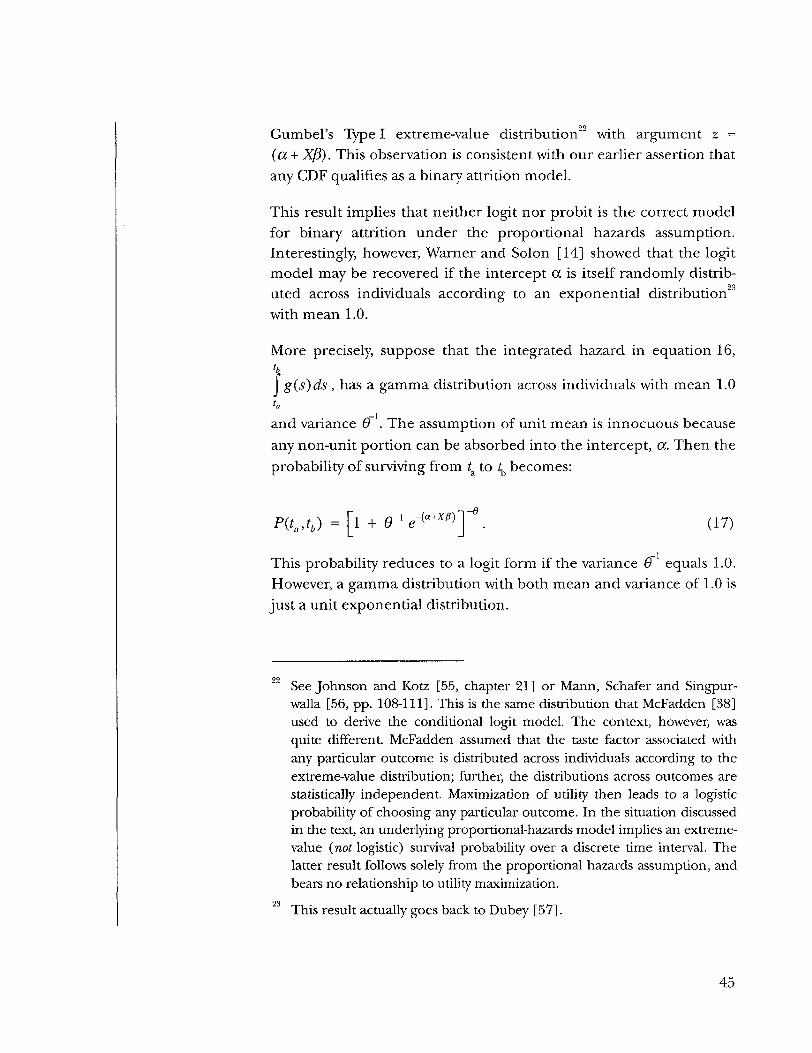
Gumbel's Type I extreme-value distribution2" with argument z =(a + Xfl). This observation is consistent with our earlier assertion thatany CDF qualifies as a binary attrition model.

This result implies that neither logit nor probit is the correct modelfor binary attrition under the proportional hazards assumption.Interestingly, however, Warner and Solon [14] showed that the logitmodel may be recovered if the intercept a is itself randomly distrib-uted across individuals according to an exponential distribution23

with mean 1.0.

More precisely, suppose that the integrated hazard in equation 16,

g(s)ds, has a gamma distribution across individuals with mean 1.0

and variance 9 . The assumption of unit mean is innocuous becauseany non-unit portion can be absorbed into the intercept, a. Then theprobability of surviving from t^ to ^ becomes:

p(ta,tb) =This probability reduces to a logit form if the variance 6 equals 1.0.However, a gamma distribution with both mean and variance of 1.0 isjust a unit exponential distribution.

See Johnson and Kotz [55, chapter 21] or Mann, Schafer and Singpur-walla [56, pp. 108-111]. This is the same distribution that McFadden [38]used to derive the conditional logit model. The context, however, wasquite different. McFadden assumed that the taste factor associated withany particular outcome is distributed across individuals according to theextreme-value distribution; further, the distributions across outcomes arestatistically independent. Maximization of utility then leads to a logisticprobability of choosing any particular outcome. In the situation discussedin the text, an underlying proportional-hazards model implies an extreme-value (not logistic) survival probability over a discrete time interval. Thelatter result follows solely from the proportional hazards assumption, andbears no relationship to utility maximization.

This result actually goes back to Dubey [57].

45

Warner and Solon estimated a model of this form to predict survivalto the first-term reenlistment decision point (though not the exactmonths-of-service if the individual attrites), jointly with a probitmodel to predict first-term reenlistments among those surviving tothe reenlistment decision point. They allowed for correlation be-tween the disturbances in the two models, but found that the correla-tion was not statistically significant.

Continuous-time models of attrition and reenlistmentYet another alternative would be to estimate a single, continuous-timemodel to predict the exact months-of-service at which a person:

• Attrites before the reenlistment decision point; or

• Survives to the reenlistment decision point, but decides toseparate at that point; or

• Survives to the reenlistment decision point, and decides to re-enlist at that point, but separates at some subsequent point[either before or at the individual's updated expiration ofterm-of-service (ETS)].

When estimating this type of model, one danger is that the propor-tional hazards assumption constrains the regressor effects to be thesame in the attrition phase as in the reenlistment phase. For example,suppose that a particular dummy variable (perhaps identifying a par-ticular demographic group) has a coefficient of 0.15. This coefficientindicates that members of the highlighted group are 14 percent lesslikely than members of the base group to separate at any point in time(conditional on survival to that point). However, using separate attri-tion and reenlistment models, Warner and Solon found that highschool graduates (HSGs) are more likely than nongraduates to surviveto the reenlistment decision point, but less likely than nongraduates to

A coefficient of 0.15 serves to scale down the hazard function by the factore ' ° = .86, a 14-percent reduction. It is convenient—but imprecise—to as-sociate, for example, a coefficient of 0.15 with a 15-percent reduction.

46

reenlist. Clearly, no single coefficient on HSG status could captureboth effects.

Follmann, Goldberg, and May [13, 58] addressed this problem by de-veloping a continuous-time model with different regressor effectsalong different intervals of the time axis. In their example, they mod-eled the probability of an unemployed worker finding a job as afunction of the duration of his or her unemployment spell. A dispro-portionate number of unemployed workers find jobs during the weekthat their unemployment insurance (UI) benefits expire, typically the26th or 39th week of the unemployment spell. This phenomenoncould apparently be accommodated using a proportional hazardsmodel with a nonmonotonic step function, g(t). However, the con-ventional proportional-hazards model constrains the regressor effectsto be the same throughout the entire time axis.

Instead, Follmann, Goldberg, and May modeled the probability offinding a job as an extreme-value regression (equation 16) duringthe week that UI benefits expire. They modeled the probability offinding a job using a conventional proportional-hazards model overthe remainder of the time axis. Importantly, they allowed for differ-ent regressor effects over the two time intervals. Indeed, they foundthat college graduates residing in counties with low unemploymentrates were most likely to find jobs during the week their UI benefitsexpire; but that older, white workers were more likely to find jobs atall other times.

Although similar in spirit, there are some important differences be-tween the approaches of Follmann et al. and Warner and Solon.Follmann et al. define the "spike event" as the period during whicha disproportionate number of transitions occur. In their example,the spike event was the week in which UI benefits expire. If appliedto attrition and reenlistment in the military, the spike event wouldbe the period immediately preceding ETS. They modeled theprobability of a spike event using extreme-value regression, al-though other models, such as logit or probit could have been usedinstead. They modeled events away from the spike using a continu-ous-time, proportional-hazards model. The advantage of using ex-treme-value regression is that the coefficient vector /? in

47

equation 16 is commensurable with the corresponding coefficientvector in the proportional-hazards model (equation 15) away fromthe spike. Although Follmann et al. allowed the two coefficient vec-tors to differ, it remains meaningful to statistically test their equal-ity. A similar result would hold if generalized logit regression(equation 17) were used in place of extreme-value regression at thespike. However, a probit coefficient vector at the spike would bescaled differently from the coefficients in the proportional-hazardsmodel, and the two could not easily be tested for equality.

Warner and Solon modeled their spike event—reenlistment duringthe period immediately preceding ETS—using probit regression.They modeled attrition away from the spike as a binary outcome us-ing, variously, probit, logit, or generalized logit regression (i.e.,equation 17). However, they did not estimate the entire, continu-ous-time hazard function, g(t). Instead, they estimated the annualsurvival rates for the baseline demographic group (i.e., the groupwith regressors X = 0 ) . The annual survival rates are the values ofexpression 17 when evaluated at successive annual intervals; i.e.,(^J = {(0,1),(1,2),(2,3),(3,4),}.25 Thus, Warner and Solon claimtoo much when they state [14, p. 263], "The main advantage of theproportional hazard results is that they trace out the temporal pat-tern of attrition." By estimating only the annual survival rates,rather than the entire hazard function g(t), their resolution is lim-ited to an annual view of the attrition process. The month-to-month hazard function could have been estimated using, for ex-ample, the Kaplan-Meier nonparametric procedure.

The approaches of Follmann et al. and Warner and Solon both havemerit, and it would be interesting to compare their performance on acommon data set. Off-the-shelf statistical software could be used if the

25 The annual hazard rates are obtained from the parameters a, through a(

r -i i ~°in table 6.7 of [12], using the transformation 1 + 0 exp(-a,) . Thesurvival rates are obtained by cumulating the annual hazard rates.

See Kalbfleisch and Prentice [54, pp. 10-16].

48

reenlistment decision were modeled using logit or probit regression."'However, extreme-value regression would require specialized software,and incorporation of a permanent-transitory error structure would beeven more difficult.

27 The earlier paper by Follmann et al. [13] actually made a start in this di-rection, examining attrition of non-prior-service Marine Corps reservists.At the time that paper was written, the authors were not yet aware of thespecial commensurability between extreme-value regression and theproportional-hazards model. Thus, they used logit regression rather thanextreme-value regression at the spike (the end of the 4-year contract);and a Weibull model rather than a proportional-hazards model awayfrom the spike. Nonetheless, they found that distinct subsets of regres-sors had significant effects on the hazard function at the spike versusaway from the spike.

28 Extreme-value regression could be estimated using LIMDEP. See chapter21.7, "User Defined Index Models for Binary Choice," in the on-linemanual for LIMDEP version 7.0 (www.limdep.com).

49

THIS PAGE INTENTIONALLY LEFT BLANK

Elasticity computationCare must be exercised in computing the elasticity of reenlistmentwith respect to military pay. The elasticity is sensitive to both the defi-nition of "reenlistment" and the definition of "military pay."

Definition of reenlistmentThe definition of "reenlistment" is complicated by the followingf 29factors:

• Early attrition

• Early reenlistment

• Reenlistment eligibility

• Extensions

• Reenlistments to retrain in a different military occupation.

Presumably, personnel who attrite before their ETS have a larger netpreference for civilian life. Failure to control for early attrition couldconfound the reenlistment model, if attrition rates are correlatedwith variables included in the model. However, Warner and Solon's[14] results imply that the correlation between attrition and re-enlistment may not be a major source of bias.

Some personnel reenlist early (e.g., more than 6 months before theirETS date), perhaps in preparation for an overseas assignment. Theirinclusion in a reenlistment model may lead to a slight bias if the payvariable is expressed in ACOL form. We have noted that ACOL valuestend to increase over a person's career. Those who reenlist early,therefore, would tend to have smaller ACOL values, leading to a

29 The next few paragraphs borrow heavily from the excellent discussion inSmith, Sylwester, and Villa [59, pp. 56-61].

51

downward bias in the ACOL coefficient. Smith, Sylwester, and Villa[59] solve this problem by evaluating ACOL at the original ETS daterather than at the early decision point.

Some personnel are declared ineligible to reenlist. Among the manyreasons are poor test scores, failure to meet medical or physical fit-ness standards, disciplinary problems, or missed promotions. Onetemptation is to exclude these people from any model of voluntaryreenlistment. There are two counterarguments, however. First, somepeople are declared ineligible after expressing a disinclination to re-enlist (e.g., turning down a required overseas assignment). Excludingsuch people will overstate the reenlistment rate, and may also con-found the model estimates if eligibility is correlated with variables inthe model. Second, for the purposes of force planning, models thatinclude ineligibles are probably more valuable because the totalpopulation at ETS (including ineligibles) is the base to which pre-dicted reenlistment rates are generally applied.

Extensions have already been discussed at length. One difficulty withsome of the older studies is that they do not document their treat-ment of extensions. For example, some studies drop extensions en-tirely and model the dichotomy between immediate reenlistmentsand separations. Other studies combine extensions with reenlist-ments and model total retention. Still other studies track extensionsto determine whether they ultimately reenlist, thus retrospectivelyclassifying extensions as either reenlistments or separations. It is dif-ficult to compare the elasticities from studies that differ in theirtreatment of extensions.

Finally, individuals who reenlist to retrain in a different military oc-cupation are not eligible to receive an SRB. Not all studies (particu-larly those using grouped data) correctly identify this group. Thus,the military pay variables are measured with error, and the pay coeffi-cients may be downward biased.

Definition of military payWe now turn to the definition of "military pay." Warner and Goldberg[18, p. 33] describe the preferred method to compute a pay elasticity:

52

The pay elasticity is calculated as the percentage increase inthe reenlistment rate brought about by a one-level SRB in-crease, divided by the percentage increase in [annualizedmilitary pay] implied by the SRB increase.10

Along similar lines, Smith et al. [59, p. 86] construct a "typical mili-tary pay raise" as a simultaneous 1-percent increase in basic pay, basicallowance for subsistence (BAS), and basic allowance for quarters(BAQ). These methods are preferred because the increase in militarypay is measured as a percentage relative to the base value of militarypay, and the latter is always strictly positive.

When the retention model is estimated from individual data, it ispreferable to compute the increase in the reenlistment probabilityfor each person in the sample and then aggregate, rather than towork directly with the sample averages. For example, a 1-percent in-crease in military pay might lead to a 1.0-percent increase in the re-enlistment probability for one person, a 1.5-percent increase for asecond person, and so on. The simple average of these probabilityincreases should be used to form the numerator of the elasticity. Us-ing, instead, the percentage increase in the reenlistment probabilityfor the "average" person is less accurate and—because the model isnonlinear—could lead to a numerically different answer.

Some other studies compute the pay elasticity with a denominator equalto the percentage change in the military/civilian pay difference. For exam-ple, Daula and Moffitt [60] measure the percentage change in reenlist-ment generated by a (presumably sustained) increase in themilitary/civilian pay difference: A (M- C) / (M- C). In a later paper,Daula and Moffitt [24] make the same computation for some of their es-timates. However, they also report elasticities using the Warner/Goldberg

Under the installment arrangement, the annual SRB payment equals anSRB "level" or "multiple" (an integer or half-integer in the range 0 to 6) xmonthly basic pay at the date of reenlistment. Under the lump-sumarrangement, the single payment equals the product of the SRB level,monthly basic pay, and the number of years of reenlistment. In either case,a one-level SRB increase implies an increase in undiscounted dollars equalto monthly basic pay x number of years of reenlistment. However, this in-crease is enjoyed only by reenlisting, not by merely extending.

53

method, increasing military pay alone: AM/ M. They even report elastic-ities using the percentage change in ACOL, ziACOL/ACOL, and thepercentage change in the total (not annualized) discounted pay differ-ence over a predetermined (not necessarily "optimal") horizon (their so-called Total Cost of Leaving or TCOL).

Elasticities estimated by these latter methods are unstable, andshould not be used for policy evaluation. A pay difference near zeroimplies a zero elasticity; even a slightly negative pay difference im-plies a negative elasticity, even when retention and military pay movein the same direction. To see these points, consider the elasticitywhen the denominator is measured relative to the military/civilianpay difference:

[AP/ P]/ [A (M- C) / (M- Q]

= [(M-Qx (APj\ / [PxA(M-C)]. (18)

Suppose that the base military/civilian pay difference happens toequal zero. Then the percentage change appearing in the denomina-tor on the left-hand side is infinite, implying that the elasticity itself(the entire right-hand side) equals zero. As another example, if thebase military/civilian pay difference is negative, the elasticity will alsobe negative, even if increased pay has a positive effect in encouragingmore reenlistments (i.e., even if the changes A P and A (M- C) havethe same algebraic sign). In neither case is the computed elasticityuseful for policy evaluation. Our situation is unique because, unlikemost policy evaluations, the base value of our independent variabledoes not always take the same algebraic sign, leading to instability inthe conventionally computed elasticity.

Finally, recall that Hosek and Peterson [12] used two compensationmeasures: the 8KB level and an index of relative military pay. They re-port the percentage-point increase in the reenlistment rate associatedwith a one-level 8KB increase. Although not an elasticity, the interpre-tation of this quantity is straightforward.

Hosek and Peterson also report the percentage increase in the reten-tion (i.e., reenlistment plus extension) rate associated with a1-percentage-point increase in the military/civilian wage index.

54

Unless the base value of the wage index is 1.0, a 1 percentage-point in-crease in the wage index does not equate to a 1-percent increase. Infact, the mean value of the wage index was 0.94 in Hosek and Peter-son's sample. Thus, to obtain the elasticity of retention with respectto relative military pay, their reported percentage increase in the re-tention rate must be multiplied by the factor 0.94.

31 This correction is sometimes neglected, for example, by Warner andAsch [61, table 5].

55

THIS PAGE INTENTIONALLY LEFT BLANK

Elasticity estimates

Pay elasticitiesTable 2 summarizes the pay elasticities from various studies. The left-hand panel shows the elasticity of the reenlistment rate (or, in somecases, the total retention rate) with respect to some measure of mili-tary pay. As we have discussed, the most stable estimates use militarypay alone, rather than the military/civilian pay difference, in the de-nominator of the elasticity. We will limit our discussion to the formerestimates.

Goldberg and Warner [30] report first-term pay elasticities in therange of 1.1 to 2.7, whereas Warner and Goldberg [18] report a simi-lar range of 1.1 to 3.4. Considering the other studies that use militarypay alone in the denominator, most of the elasticities cluster withinthe even narrower range of 1.2 to 2.2. These other studies includeCooke, Marcus, and Quester [16], Daula and Moffitt [24], Shiells andMcMahon [17], Smith et al. [59], and Warner and Solon [14]. All ofthe studies cited in this paragraph use individual data, except forGoldberg and Warner [30], who use grouped data.

Three studies do not conform to this pattern, instead reporting con-siderably lower first-term pay elasticities. Mackin et al. [27] estimatedpay elasticities by Navy occupational group. Even their most respon-sive occupational group had an elasticity of only 1.5. Two of the stud-ies used the ACOL-2 approach, but correctly computed the payelasticities with respect to military pay alone, rather than with respectto the ACOL pay difference. Mackin [62] reports elasticities by ser-vice, ranging from 0.5 to 1.4. Black, Hogan, and Sylwester [31] reportan elasticity of 0.8 to 0.9 for Navy enlisted personnel. As we discussedearlier, the ACOL-2 approach was designed, in part, to correct an

57

oo Table 2. Pay elasticities from various studies

Study

Black, Hogan, andSylwester [31]

Cooke, Marcus,and Quester [16]

Daula and Moffitt[60]Daula and Moffitt[24]

Goldberg andWarner [30]

Gotz and McCall[9]

Hosek andPeterson [12]

Pay variable

ACOL-2;but elasticity ofreenlistmentwith respect tomilitary payMilitary/ civilianpay index;SRBMilitary/civilianpay differenceMilitary/civilianpay differenceMilitary payaloneACOL-2Total retention;military payalone (RMC)Military/civilianpay difference

Military/civilianpay index; SRB

Sample SRB effect on reenlistment (not total retention) raterestrictions Pay elasticity (PP>S = percentage points)

First- Second-term term First-term Second-term

Installment Lump-sum Installment Lump-sumNavy enlisted 0.8 - 0.9 0.3

Navy enlisted 1.6 2.5 pp's

Army infantry 1.2

Army infantry 0.5 0.5

Army infantry 2.2 1.3

Army infantry 0.8 0.6Navy enlisted, 1.1-2.7 0.9-3.8 1.5 - 3.0 pp's 2.0 -3.9 pp's 1.6 -9.1 pp's 2.1 -11.4 pp'sby occupa-tional groupUSAF pilots, 0.8YOS 7-8USAFnon- 1.4rated officers,YOS 6-7Enlisted males, 3.6 1.6 1.8 pp's 2.5 pp's 2.3 pp's 2.2 pp'sfour services

Table 2. Pay elasticities from various studies (continued)

Study

Mackin [62]

Mackinetal. [27],conditional logitmodel

Shiells andMcMahon [17]

Smith et al. [59]

Warner andGoldberg [18]

Warner and Solon[14]

ACOL-2;but elasticity ofreenlistmentwith respect tomilitary payReenlistment;military payaloneTotal retention;military payaloneMilitary/ civilianpay index;SRBMilitary payalone

Military payalone (SRB)

ACOL;but elasticity ofreenlistmentwith respect tomilitary pay

Samplerestrictions

Army enlistedNavy enlistedUSAF enlistedUSMC enlisted

Navy enlisted,by occupationalgroup

Navy enlisted

Army infantry

Army maintenanceArmy administrationNavy enlisted,by occupationalgroupArmy infantry

| SRB effect on reenlistment (not total retention) ratePay elasticity i (PP>S = percentage points)

First- Second- iterm term i First-term Second-term

I Installment Lump-sum Installment Lump-sum1.2 1.0 !1.0 0.8 |0.5 0.4 |1.4 1.1 |

0.2-1.5 0.5-1.1 ! 0.4-2.8pp's 1.9-2.6pp's

0.2-0.9 0.5-1.0

1.9 | 1.5pp's

1.3 0.9 1 2.2pp's 1.7pp's

1.8 1.1 i1.9 1.8 i

1.1-3.4 | 1.8-5.5pp's

1.2 !

Notes: pp's = percentage points, USAF = United States Air Force, USMC = United States Marine Corps, YOS = years of service.

UT

upward bias in simple ACOL models when applied at the second-term (or later) decision points. Thus, we would expect the ACOL-2approach to yield lower pay elasticities for these later decisions. How-ever, it is surprising that the approach yields such lower pay elastic-ities at the first-term decision point.

Figure 7 plots the various first-term pay elasticities. In constructingthis figure, we arrayed the elasticities from left to right, alphabeticallyby the last name of the first author, except that we grouped theACOL-2 studies to the extreme right. For studies that estimatedseparate elasticities by occupational group, we used a vertical bar todepict the range of elasticities, and a circle to indicate the midpointof the range. We see that there is considerable dispersion in the elas-ticity estimates, but the ACOL-2 estimates tend to be concentrated atthe lower end.

Figure 7. Elasticity of first-term retention with respect to pay

>,

'•s

CL

3

o

22.

100

u -5 -0 -5 -0 -_

0 -*jo -I

10

\\

. . . . ft . . . .

(

?\\

<

* . *•

\\\\\^^>^\^%;

ACOL-2

• •..... .. .. . . . . . . . . . . . f . . . . . . . . . . . .. . . . . . ............................

^f- ^f- <$• <J> 4-., •£•, 4"1, -^\ \ \ % %. %. \.\.\\%^ \\>v%\ W^;\Authors

We now turn to the second-term pay elasticities. Goldberg and Warner[30] report pay elasticities in the range of 0.9 to 3.8. Daula and Moffitt[24] and Smith et al. [59] report pay elasticities that cluster within theconsiderably narrower range of 0.9 to 1.8. Mackin et al. [27] reportsomewhat lower pay elasticities, in the range 0.5 to 1.1. Using theACOL-2 approach, Mackin [62] reports elasticities by service ranging

60

SRB effects

from 0.4 to 1.1. Finally, Black, Hogan, and Sylwester [31] report anelasticity of only 0.3 for Navy enlisted personnel.

In figure 8, we plot the second-term pay elasticities. Not surprising inthis case, the ACOL-2 estimates again tend to be concentrated at thelower end.

Figure 8. Elasticity of second-term retention with respect to pay

3 r-

2 p-

2 f\

1.0-

0.0-

(

•

\

. • A COL-2. . . . . . . . . . . . L... . ..9... .................... .9... . . . . . . . . . . . . . . . . .

. . . . . . . . ...i. . . . ' . . . . . . . . . . . . . . . . . . . . . . . .«.. . . . . . . . . .• . . . . , . . . . . . . .

\ \ \ % % % \ s \ \ \ \?> '2>/- </^3, < i '%'. ^ ^ d^ ty ^&> ^p ^p ^

^5, ^^ ,- *^x v/ 51,<?2, '( 'f ij, 'j, -

Authors

Table 2 also summarizes the effect of a one-level SRB increase on thereenlistment (not total retention) rate. The most interesting compari-son is between the two studies that used grouped data: Goldberg andWarner [30], who estimated a conditional logit model, and Hosek andPeterson [12], who estimated a multinomial logit model. According toGoldberg and Warner, a one-level increase in the first-term SRB, if paidin annual installments, serves to increase the reenlistment rate by 1.5to 3.0 percentage points. Hosek and Peterson's point estimate of 1.8percentage points falls within this range. Similarly, Goldberg and War-ner report second-term installment SRB effects in the range of 1.6 to9.1 percentage points; excluding a high outlier narrows the range to1.6 to 5.2. Hosek and Peterson's point estimate of 2.3 percentagepoints falls within that range. The other studies tend to confirm theranges established by Goldberg and Warner. Three other studies [16,

61

17, and 59] report first-term SRB effects in the range of 1.5 to 3.0percentage points. Both Mackin et al. [27] and Warner and Goldberg[18] estimated SRB effects by Navy occupational group. In both cases,the occupational groups were rather dispersed, with a few producingSRB effects outside the range of 1.5 to 3.0. The first-term SRB effectsare plotted in figure 9.

Figure 9. Effect of one-level SRB increase on first-term reenlistment rate

6.0 T

5.0 - ••

4.0 - -

I «a> ro 3.0 - - - -m Sin

2.0 - -

1.0 -••

0.0Cooke[16] Goldberg [30] Hosek [12] Mackin [27] Shiells[17] Smith [59] Warner [18]

infantry

Authors

The second-term SRB effects are plotted in figure 10. All of thesecond-term SRB effects fall within the range of 1.6 to 5.2 percentagepoints established by Goldberg and Warner. In fact, the other esti-mates cluster within the considerably narrower range of 1.7 to 2.6percentage points.

Combining the first-term and second-term results, it appears as arough rule of thumb that a one-level SRB increase leads to an in-crease in the reenlistment rate of about 2 percentage points.

62

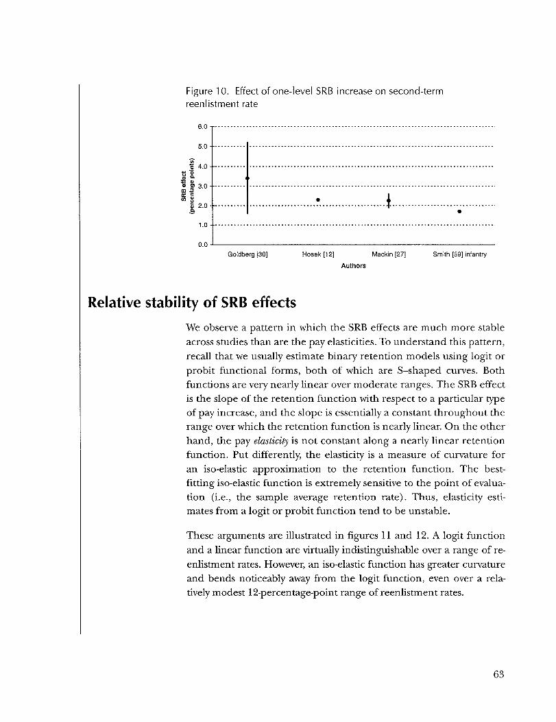
Figure 10. Effect of one-level SRB increase on second-termreenlistment rate

mCC<n

I

o.v

4.0 -

2.0 -

1.0-

n n -

i

1

Goldberg [30] Hosek[12] Mackin [27]

Authors

Smith [59] infantry

Relative stability of SRB effectsWe observe a pattern in which the SRB effects are much more stableacross studies than are the pay elasticities. To understand this pattern,recall that we usually estimate binary retention models using logit orprobit functional forms, both of which are S-shaped curves. Bothfunctions are very nearly linear over moderate ranges. The SRB effectis the slope of the retention function with respect to a particular typeof pay increase, and the slope is essentially a constant throughout therange over which the retention function is nearly linear. On the otherhand, the pay elasticity is not constant along a nearly linear retentionfunction. Put differently, the elasticity is a measure of curvature foran iso-elastic approximation to the retention function. The best-fitting iso-elastic function is extremely sensitive to the point of evalua-tion (i.e., the sample average retention rate). Thus, elasticity esti-mates from a logit or probit function tend to be unstable.

These arguments are illustrated in figures 11 and 12. A logit functionand a linear function are virtually indistinguishable over a range of re-enlistment rates. However, an iso-elastic function has greater curvatureand bends noticeably away from the logit function, even over a rela-tively modest 12-percentage-point range of reenlistment rates.

63

Figure 11. Logit function is closer to linear than to iso-elastic

0.70 -

0.60 -

„ 0.50 -2| 0.40 HEI 0.30 H

a>0.20 -

0.10 -

0.000

SRB level

Figure 12 increases the magnification within a plausible range of re-enlistment rates. The logit function is essentially linear, with a slopeof 0.02 reflecting the 2-percentage-point increase in the reenlistmentrate with each unit increase in the SRB level. Also shown are threeiso-elastic curves with very different elasticities. A small perturbationin the point of evaluation can lead to a nearly threefold variation inthe pay elasticity.

Figure 12. Point estimates of elasticities are unstable

64

The studies summarized in table 2 vary considerably in the sampleaverage retention rate. The theoretical threefold variation in payelasticities is supported by figure 7: most of the first-term elasticitiesfall within the range of 1.2 to 2.2, but a few fall below 1.0, and othersexceed 3.0. Thus, while the SRB effects are relatively stable, the payelasticities are rather unstable. If either, it is the former that is closerin character to a "natural constant."

65

THIS PAGE INTENTIONALLY LEFT BLANK

Estimation of discount ratesHosek and Peterson [12, p. 1] state that, "The chief purpose of[their] study is to determine whether lump-sum reenlistment bo-nuses are more cost-effective than installment bonuses." The primaryfactor in this determination is a comparison of discount rates be-tween military members and the federal government. Interestingly,Hosek and Peterson did not use their findings to explicitly infer amilitary member's discount rate. Nonetheless, they argued that lump-sum reenlistment bonuses are cost-effective as long as the federal gov-ernment's real discount rate lies anywhere in the range of 4 to10 percent. Their report appeared during a period when OMB wasstill mandating use of a 10-percent real discount rate on governmentinvestment projects. Thus, they concluded that lump-sum bonusesare the preferred method of payment. "

Hosek and Peterson exploited a natural experiment that occurred inApril 1979, when the method of SRB payment switched from annualinstallments to lump-sum payments. They estimated both a dichoto-mous model of staying (i.e., either reenlisting or extending) versusleaving, and a trichotomous model of reenlisting, extending, or leav-ing. They found that, in the former case, installment bonuses wereonly 82.7 percent as effective as lump-sum bonuses in encouragingfirst-term enlisted personnel to stay. In the latter case, installmentbonuses were 72.8 percent as effective as lump-sum bonuses inencouraging first-term personnel to reenlist. We can use thesefindings to roughly estimate a military member's real discount rate.

According to economic theory, individuals make their decisions bycomparing the discounted present values of the various alternatives.

In 1992, OMB revised its guidance and tied the real discount rate toinflation-adjusted market rates on Treasury bonds. Those rates have gen-erally been in the range of 3 percent to 4 percent. The rationale forOMB's revised guidance was provided after the fact by Goldberg [63].

67

If installment bonuses are only 72.8 percent as effective as lump-sumbonuses, the present value of the former must be only 72.8 percentthe present value of the latter. Assume a 4-year reenlistment horizonand, following Hosek and Peterson, a 95-percent annual survival ratewithin the second term of service. Considering a notional $1,000 bo-nus, we have the following present-value equation:

0.728 x $1,000= $250x{l + 0.95/(l+r; + [0.95/(l+r)f + [0.95/(l+r)]3>. (19)

Note that we have not deflated the $250 annual installments by aprice index, so that the installment stream is expressed in nominal(i.e., current) dollars. Therefore, the solution to this equation pro-vides an estimate of the nominal discount rate.33 The solution is easilycomputed as 20.1 percent. Repeating the exercise using a relative ef-fectiveness of 82.7 percent (based on the dichotomous model) yieldsa nominal discount rate of 8.7 percent.

To convert to real discount rates, we use the following relationshipbetween the nominal discount rate (r), the real discount rate (d), andthe rate of inflation (f):

(l + r)=(l + d)x(l+f). (20)

33 Hosek and Peterson's analysis appears to contain an error. Their equa-tion on p. 42 of [12] is essentially the same as our equation 19. They ex-press the annual installment bonus in nominal terms, as 25 percent ofthe corresponding lump-sum bonus. To properly discount the stream ofinstallment payments, they should be using a nominal discount rate. How-ever, they state on p. 43, "In keeping with our having adjusted the bonusamounts in the empirical work for inflation, the interest rate [that solvesthe equation] should be interpreted as the 'real' rate—that is, theinflation-adjusted rate." This statement is a non sequitur; having normal-ized the various years' bonus amounts in the regression analysis does notrelieve the requirement to either discount a nominal payment streamwith a nominal discount rate, or a real payment stream with a real dis-count rate. Hosek and Peterson attribute to real discounting all of themilitary member's preference for a lump-sum bonus. In fact, some ofthat preference should instead be attributed to the automatic inflationprotection provided by an immediate, lump-sum payment.

68

Over the sample period of FY 1976 through FY1981, the geometricaverage rate of increase in the Consumer Price Index (CPI) was 9.2percent. Applying the above formula, we estimate real discount ratesof 9.9 percent from the trichotomous model and -0.5 percent fromthe dichotomous model. Cylke et al. [15] argue that consideration ofprogressive income taxes tends to increase the estimated discountrate. We have not performed the detailed analysis of Hosek and Pe-terson's results, including tax effects. However, their results implythat military members' real discount rates are surely positive, andmay well exceed 10 percent.

Other discount-rate estimatesTable 3 summarizes the real discount rates estimated from variousstudies. Cylke et al. [15] followed a procedure similar to Hosek andPeterson, comparing the effectiveness of SRBs when paid in annualinstallments (pre-April 1979) versus a single lump-sum (post-April1979). Daula and Moffitt, by contrast, used the method of maximumlikelihood to estimate the discount rate as one parameter in the dy-namic program. Warner and Fleeter [64] compared military mem-bers' choices between installment and lump-sum severance pay whenthe two were offered concurrently; we will discuss their study in thenext section.

Table 3. Estimates of real discount rates

StudyCylke etal. [15]Daula and Moffitt [60]

Daula and Moffitt [24]Hosek and Peterson [12]

Warner and Fleeter [64]

Sample restrictionsNavy enlistedArmy infantryArmy infantryArmy infantryenlisted males,four servicesArmy, Navy,Air Force officersArmy, Navy,Air Force enlisted

Term of service1st term only1st term only1st and 2nd terms1st and 2nd terms1st term only

YOS 7 through 15

YDS 7 through 15

Real discount rate17%

4.0% - 5.5%10.5%

10% - 14%9.9%

6% - 26%

26% - 37%

Note: Real discount rate from Hosek and Peterson [12] is inferred in the current paper.

69

Looking across all of the studies, the estimated discount rates rangebetween 4 and 37 percent. However, excluding Daula and Moffitt's[60] low first-term estimates, as well as Warner and Pleeter's high es-timates for enlisted personnel, the remaining estimates range be-tween 6 and 26 percent. These rates all exceed the federalgovernment's real discount rate of 3 to 4 percent, leaving little doubtthat lump-sum bonuses are the preferred method of payment.

Warner and Fleeter studyWarner and Fleeter [64] exploited a natural experiment that oc-curred when DoD reduced military endstrength during FY 1992 andFY 1993. Recall that both Cylke et al. and Hosek and Peterson com-pared a time period during which SRBs were paid in annual install-ments to a time period during which SRBs were paid as a singlelump-sum. By contrast, Warner and Fleeter examined a single timeperiod during which both installment and lump-sum severance paywere offered concurrently. What makes their study unique is thatmilitary members were offered a contemporaneous choice between thetwo payment options.

Specifically, DoD offered severance packages to mid-career personnel(both officer and enlisted) in selected combinations of military occu-pation, paygrade, and years of service. The Voluntary Separation In-centive (VSI) provided annual payments equal to 2.5 percent ofterminal basic pay, multiplied by terminal years of service. The annualpayments would continue for a period of time equal to twice the ter-minal years of service, with no indexing for inflation. The SpecialSeparation Benefit (SSB) provided a lump-sum payment equal to 15percent of terminal basic pay, multiplied by terminal years of service.34

Mehay and Hogan [65] report that, during FY 1992, less than 10 percentof the Navy enlisted force met the occupation/paygrade/YOS eligibilitycriteria. Among these individuals, 12 percent accepted some form ofbuyout. Mehay and Hogan did not explicitly analyze the choice betweenthe two payment options. However, they report that among Navy enlistedpersonnel who accepted some form of buyout, 85 percent chose the SSB(lump-sum) payment option.

70

If individuals did not discount, the annuity option would be pre-ferred as long as YOS > 3 (for then 2.5% x basic pay x YOS x 2 x YOS> 15% x basic pay x YOS). With discounting, the breakeven careerlength is somewhat longer. Put differently, for any given career lengthof YOS > 7 (the minimum for buyout eligibility), one can comparethe discounted present values of the two payment options at variousdiscount rates. In fact, when announcing the program, DoD pub-lished a pamphlet giving the comparison of present values at a7-percent nominal discount rate, which was the typical yield onmoney market funds at the time. Using that discount rate, the pre-sent value of the annuity option was as much as twice the size of thelump-sum payment.

One can also calculate the breakeven discount rate—the rate atwhich a person must discount the annuity payments to yield a presentvalue equal to the lump-sum payment. Warner and Fleeter computedbefore-tax breakeven discount rates ranging from 17.5 to 19.8 per-cent, varying solely as a function of YOS. They also computedafter-tax breakeven discount rates ranging from 17.5 to 23.6 percent.

Despite these high breakeven rates, most people chose the lump-sumpayment option, indicating that their personal discount rates wereeven higher. According to Warner and Fleeter:

Among the officers with less than 10 years of service, morethan half took the lump-sum. Among the E-5 enlisted per-sonnel with less than 10 years, over 90 percent did so. Al-most 75 percent of E-7 enlisted personnel with 15 years ofservice took the lump-sum. Even among the more senior of-ficers, 30 percent or more took the lump-sum. Overall,about half of the officers chose the lump-sum while over 90percent of the enlisted personnel did so.

Warner and Pleeter's estimated discount rates were shown earlier intable 3. They ranged from 6 to 26 percent for officers, and from 26 to37 percent for enlisted personnel.

We use some diagrammatic tools from microeconomic theory to illu-minate these calculations. Figure 13 is an indifference-curve diagramfor a person choosing between the annuity and lump-sum payment op-tions. The axes measure consumption of goods and services in the first

71

and second time periods, respectively. Absent either severance pay oraccess to financial markets, the person would simply consume his orher income in each period. This income "endowment" is depicted aspoint E. Relaxing these assumptions gradually, suppose next that theperson may either borrow or lend at the interest rate r. The resultingbudget line passes through point E with negative slope of 1 + r. As thefigure is drawn, this individual would choose to lend money in the firstperiod, reducing consumption in that period but increasing consump-tion in the second period when the investment comes due. Geometri-cally, the person moves along the budget line from point E to aconsumption optimum at point B.

Figure 13. Comparison of annuity and lump-sum payment options

tc, u

45C

slope = 1 + r

C,

The slope of the person's indifference curve at point B equals 1+r.Thus, the observed slope is solely a function of the interest rate atwhich the person may either borrow or lend. The observed slope is

72

not a measure of underlying preference for current versus future con-sumption. The latter must be measured at some benchmark level ofrelative consumption that is independent of market opportunities.Conventionally, a measure of time preference (or "impatience") isderived from the slope of the person's indifference curve at the45-degree line (the line along which current and future consumptionare equal). The slope at the 45-degree line (e.g., at point A) isequated to 1 + p, and p is defined as the consumer's "rate of time

r »35preference.

To see this point in another way, consider the two individuals pic-tured in figure 14. These two have very different preferences for cur-rent versus future consumption. The "impatient" one is moreconcerned with current consumption, and has a steep indifferencecurve (drawn as a solid curve). By contrast, the "patient" person ismore concerned with future consumption, and has a flat indifferencecurve (drawn as a dashed curve). These differences in time prefer-ence are evident by comparing the slopes of the solid and dashed in-difference curves at the 45-degree line. Yet, if these two peopleborrow or lend at the same interest rates as each other, they willreach consumption optima at which each has an indifference curvewith slope 1 + r. Again, the observed slope measures market oppor-tunities rather than underlying time preference.36

Finally, we compare the annuity and lump-sum severance packages.Returning to figure 13, the annuity option serves to increase incomeduring both the first and second periods. Thus, the annuity optionshifts the endowment point both horizontally (point F) and then ver-tically (point G). The new budget line passes through point G with

This definition is found in Epstein and Hynes [66], among other places.

When reviewing studies of "discount rates," one must carefully distin-guish between those that measure market opportunities (r) and othersthat measure underlying time preference (p). All of the studies in ourtable 3 are measuring market opportunities. Other studies of market op-portunities, outside the military sector, include Gately [67], Gilman [68],and Hausman [69]. Lawrance [70] is the best-known study of the con-sumer's rate of time preference.

73

slope 1 + r. The individual may now adjust his consumption path toreach a higher utility level at point C.

Figure 14. Two individuals with different time preferences but equalinterest rates

t

45°

By contrast, the lump-sum option serves to increase income duringonly the first period. Thus, the lump-sum option shifts the endow-ment point horizontally beyond point F, perhaps to point H. Asdrawn in figure 13, point H lies to the northeast of the budget linepassing through point G. Thus, the lump-sum option leads to an evenhigher budget line and, consequently, an even higher utility level(neither of which is explicitiy shown in the figure, to avoid clutter).

The consumer's preference for point H (lump-sum option) overpoint G (annuity option) reveals that his or her budget line is steeperthan the line segment GH. The slope of the budget line is, again,1 + r. However, the slope of the line segment GH equals 1.0 plus the"breakeven rate" computed by Warner and Fleeter. To see why, notethat points G and H would lie on the same budget line only if the twopayment options yielded exactly the same discounted present value.The line segment GH is, in fact, a subset of the hypothetical budgetline with slope equal to 1.0 plus the interest rate that equates the twopresent values—the breakeven rate.

74

As is clear from this analysis, the consumer prefers the lump-sum pay-ment option only if his or her personal discount rate exceeds thebreakeven rate. Thus, a consumer's choice of either the annuity orlump-sum payment option serves to bound his or her personal discountrate on one side or the other of the predetermined breakeven rate. It isthis information that Warner and Fleeter exploit to estimate the distri-bution of personal discount rates in the military population.

75

THIS PAGE INTENTIONALLY LEFT BLANK

Effects of variables other than pay

Personal characteristicsRetention models have often included variables other than pay. Per-ennial favorites include the civilian unemployment rate, and personalcharacteristics, such as marital status, race, education, and mentalgroup. One difficulty is that these are some of the same personalcharacteristics used to predict civilian pay in forming the mili-tary/civilian pay difference or pay ratio. Inclusion of these character-istics in the retention model introduces multicollinearity, which tendsto depress the estimated coefficient on the relative pay variable. Thisproblem was noted by Warner [71, pp. 222-223]:

inclusion of individual attributes such as education, race,and Armed Forces Qualification Test (AFQT) score in theretention equation to control for non-pecuniary factors re-sults in substantial changes in pay parameter estimates. Suchchanges may occur either because the model is properlyspecified only with these variables included or because ofthe multicollinearity introduced, since these factors alsohelp determine the relative pay variable in the equation....Asecond source of sensitivity...may arise if variables that affectcivilian wages are also entered directly in the retention func-tion. I am not sure whether they should or should not be in-cluded. I will only comment that I have done it both ways,and I have found maximum-likelihood estimates of pay elas-ticities to be much more sensitive to inclusion or exclusionof these variables than estimates based on a grouped logitapproach.

Whether or not to include personal characteristics remains an openquestion. Personal characteristics should certainly be included ifthere is an independent interest in their effects on retention. How-ever, if the primary goal of a particular study is to estimate the pay ef-fects, it may be preferable to exclude the personal characteristicsbecause their inclusion tends to destabilize the pay coefficient.

77

Sea dutySeveral studies have examined the effect of sea duty on reenlistmentrates of sailors. Warner and Goldberg [18] modeled the first-term re-enlistment rate as a function of the expected percentage of timespent on sea duty during the second term of service. They assignedeach person the expected sea duty specific to his or her Navy rating.They estimated that a 10-percentage-point increase in prospective seaduty would reduce the reenlistment rate by a modest 1.6 percentagepoints.

The effect of sea duty was revisited by Shiells and McMahon [17]. Inthe numerical example to illustrate their findings, they increased theprospective sea/shore ratio from 2.6:1 (i.e., 2.6 years on sea duty forevery year on shore duty) to 3.3:1. They estimated that the25-percent increase in the sea/shore ratio would reduce the re-enlistment rate by 1.9 percentage points. Note that Shiells andMcMahon did not use the same metric for sea duty as did Warnerand Goldberg. Using the latter authors' metric, the percentage oftime spent on sea duty would increase from 72 percent (2.6/3.6) to77 percent (3.3/4.3). Correspondingly, the reenlistment rate wouldfall by 0.8 percentage point. Comparing the two estimates, Shiellsand McMahon's is over twice as large as Warner and Goldberg's.However, even the larger estimate implies that the hypothesized in-crease in sea duty could be offset by a one-level SRB increase.

Personnel tempoMore recently, a few studies have begun to look at the effect of per-sonnel tempo (Perstempo) on retention. Cooke, Marcus, andQuester [16] examined three measures of Perstempo for male sailors:

• Length of deployment

• Turnaround ratio, defined as time between deploymentsdivided by length of deployment

• Percentage of time under way while not deployed.

78

Reference [16] found few systematic patterns for sailors with 8 to 10years of service. However, the authors found several significant effectsamong 4-year obligors at their first reenlistment point. For instance,they found that longer deployments adversely affected retention, es-pecially among married sailors (roughly one-third of those makingreenlistment decisions). Second, a lower turnaround ratio also ad-versely affected retention, but the effect was smaller and limited tomarried sailors. Third, the percentage of time under way while notdeployed had an adverse effect on retention. The latter effect wasmost severe among both married sailors and sailors serving in rela-tively sea-intensive ratings (these two groups overlap).

Among their other results, Cooke, Marcus, and Quester [16] foundthat retention was lower among sailors deployed at their decisionpoint, even controlling for a sailor's deployment history during the 3-year window leading up to the decision point. Finally, retention waslower among sailors serving on ships that had recently undergone amajor maintenance activity (overhaul or restricted availability) thatlasted 8 months or longer.

Hosek and Totten [19] developed some additional measures of Per-stempo, and extended the analysis to all four military services. Theynot only examined long duty, but they appear to be the first to exam-ine the effect of hostile duty on retention. They measured long dutyas the incidence of the Family Separation Allowance, which is paid topersonnel with dependents from whom they are separated for 30 ormore consecutive days. They measured hostile duty as the incidenceof Hostile Fire Pay, which is paid to personnel subject to hostile fireor explosion, or those on duty in areas deemed to be hostile.

Hosek and Totten found that some degree of long or hostile duty ac-tually increases first-term retention, particularly among Army andMarine Corps personnel. Beyond a certain point, however, additionallong duty reduces retention, especially if that duty is also hostile.Therefore, overall retention might improve if the burden of long andhostile duty were shared among large numbers of military personnel.However, Hosek and Totten caution that duty sharing must be bal-anced against operational factors, including unit cohesion:

79

We found that the impact of added long or hostile duty dif-fers for personnel who have had it from those who have not,and whether it is hostile or non-hostile. Thus, if the addedhostile duty can be spread to troops who have not yet beendeployed, then the effect on reenlistment is likely to be posi-tive; if the added duty falls to those who have already beendeployed, then the effect on reenlistment is likely to benegative. Of course, decisions about how to allocate addi-tional assignments must include a variety of factors beyondeffects on retention rates. A Service's capability to sharelong or hostile duty among units may be influenced by ad-vantages gained from assigning units particular roles for amajor theater war and assuring that these units stand at fullreadiness. For readiness reasons, it may not be advisable tospread such duty more broadly (pp. xvii-xviii);...becausepersonnel are attached to units and develop specializedskills and knowledge about the unit's roles and missions,weaponry/equipment, and fellow unit members, simplyswapping one person or unit for another is essentially infea-sible. A more subtle means must be devised (p. 58).

Finally, consistent with Cooke , Marcus, and Quester [16], Hosek andTotten found much smaller effects of long or hostile duty for early-career personnel (i.e., those beyond the first term but with 10 orfewer years of service) than for first-term personnel.

80

Areas for future researchThis survey has identified several fruitful areas for future research:

• Determine what joint distribution of taste factors, if any, wouldyield the sequential logit procedure used by Warner [42] tomodel the stay/leave decision along with the reenlist/extenddecision among those who stay.

• Attempt full-information maximum-likelihood estimation ofthe nested logit model for the stay/leave and reenlist/extenddecisions.

• Add cohort-composition effects to trichotomous logit (orprobit) models for the reenlist/extend/leave decision.

• When using grouped data, explicitly model SRB levels jointlywith reenlistment rates, to control for reverse causation.

• When using individual data, apply disequilibrium estimationto distinguish supply-constrained from demand-constrainedobservations.

• Continue the joint modeling of attrition and first-termreenlistment. Compare the methods of Follmann, Goldberg,and May [58] and Warner and Solon [14] on a common dataset.

• Further investigate the apparently low first-term pay elastic-ities produced by the ACOL-2 approach.

The current paper has attempted to decompose the variation in payelasticities in terms of differences in data handling (e.g., treatment ofineligibles and extensions), modeling technique, and elasticity com-putation. However, this decomposition is confounded by differencesin service, occupational group, and time period among the manystudies examined. A useful "controlled experiment" would be to ap-ply the various estimation techniques to a common data set, therebyeliminating any confounding differences in sample composition. Inlight of the changing market for military labor, it seems imperative toconduct this experiment using the most recent available data.

81

THIS PAGE INTENTIONALLY LEFT BLANK

References[1] S. Altaian and A. Fechter. "The Supply of Military Person-

nel in the Absence of a Draft," American Economic Review,Vol. 57, 1967, pp. 19-31

[2] A. Fisher, "The Cost of the Draft and the Cost of Endingthe Draft." American Economic Review, Vol. 59, 1969, pp. 239-254

[3] Lee Hansen and Burton Weisbrod. "Economics of the Mili-tary Draft." Quarterly Journal of Economics, Vol. 82, 1967,pp. 395-421

[4] J. Miller (ed.). Why the Draft? The Case for the Volunteer Army.Baltimore: Penguin, 1968

[5] Walter Oi. "The Economic Cost of the Draft." American Eco-nomic Review, Vol. 57, 1967, pp. 39-62

[6] John H. Enns. Effect of the Variable Reenlistment Bonus onReenlistment Rates: Empirical Results for FY1971. SantaMonica, CA: RAND Corporation, Jun 1975 (R-1502-ARPA)

[7] John H. Enns. Reenlistment Bonuses and First-Term Retention.Santa Monica, CA: RAND Corporation, Sep 1977(R-1935-ARPA)

[8] Samuel Kleinman and William Shughart. The Effects of Re-enlistment Bonuses, 1974 (CNA Research Contribution 269)

[9] Glenn A. Gotz and John J. McCall. Estimating Military Per-sonnel Retention Rates: Theory and Statistical Methods. SantaMonica, CA: RAND Corporation, 1980 (R-2541-AF)

[10] Glenn A. Gotz and John J. McCall. A Dynamic RetentionModel for Air Force Officers: Theory and Estimates. SantaMonica, CA: RAND Corporation, 1984 (R-3028-AF)

83

[11] Matthew S. Goldberg. "Compensation and Retention in theU.S. Navy," doctoral dissertation, University of Chicago,1984

[12] James Hosek and Christine Peterson. Reenlistment Bonusesand Retention Behavior. Santa Monica, CA: RAND Corpora-tion, 1985 (R-3199-MIL)

[13] Dean A. Follmann, Matthew S. Goldberg, and Laurie J.May. Modeling Spikes in Hazard Rates, 1987 (CNA ResearchContribution 572)

[14] John T. Warner and Gary Solon. "First-Term Attrition andReenlistment in the U.S. Army." In Curtis L. Gilroy, DavidK. Home, and D. Alton Smith (eds.), Military Compensationand Personnel Retention: Models and Evidence. Alexandria, VA:U.S. Army Research Institute for the Behavioral and SocialSciences, 1991

[15] Steven Cylke et al. Estimation of the Personal Discount Rate:Evidence From Military Reenlistment Decisions, 1982 (CNA Pro-fessional Paper 356)

[16] Timothy W. Cooke, AlanJ. Marcus, and Aline O. Quester.Personnel Tempo of Operations and Navy Enlisted Retention,1992 (CNA Research Memorandum 91-50)

[17] Martha E. Shiells and Joyce S. McMahon. Effects of Sea Dutyand Advancement on First-Term Retention, 1993 (CNA Re-search Memorandum 92-205)

[18] John T. Warner and Matthew S. Goldberg. "The Influenceof Non-Pecuniary Factors on Labor Supply: The Case ofNavy Enlisted Personnel." Review of Economics and Statistics,Vol. 66, 1984, pp. 26-35

[19] James Hosek and Mark Totten. Does Perstempo Hurt Reenlist-ment? Santa Monica, CA: RAND Corporation, 1998 (MR-990-OSD)

[20] John T. Warner. "Analysis of the Retention Effects of theProposed Retirement System." In Supplementary Papers of the

President's Commission on Military Compensation. Washington,DC: U.S. Government Printing Office, Apr 1978

[21] John H. Enns, Gary R. Nelson, and John T. Warner. "Reten-tion and Retirement: The Case of the U.S. Military." PolicySciences, Vol. 17, 1984

[22] James H. Stock and David A. Wise. "Pensions, the OptionValue of Work, and Retirement." Econometrica, Vol. 58, Sep1990, pp. 1151-1180

[23] Robin L. Lumsdaine, James H. Stock, and David A. Wise."Three Models of Retirement: Computational Complexityversus Predictive Ability." In David A. Wise (ed.), Topics inthe Economics of Aging. Chicago: University of Chicago Press,1992

[24] Thomas V. Daula and Robert Moffitt. "Estimating DynamicModels of Quit Behavior: The Case of Military Reenlist-ment." Journal of Labor Economics, Vol. 13, No. 3, 1995,pp. 499-523

[25] Glenn A. Gotz. "Comment on the Dynamics of Job Separa-tion: The Case of Federal Employees." Journal of AppliedEconometrics, Vol. 5, 1990, pp. 263-268

[26] Matthew Black, Robert Moffitt, and John T. Warner. "Replyto Comment by Glenn Gotz." Journal of Applied Econometrics,Vol. 5,1990, pp. 269-272

[27] Patrick C. Mackin et al. U.S. Navy Enlisted Compensation andRetention Modeling. Falls Church, VA: SAG Corporation,1996

[28] David A. Wise. "Comment on Warner and Solon." In CurtisL. Gilroy, David K. Home, and D. Alton Smith (eds.), Mili-tary Compensation and Personnel Retention: Models and Evi-dence. Alexandria, VA: U.S. Army Research Institute for theBehavioral and Social Sciences, 1991

[29] John T. Warner and Bruce Simon. An Empirical Analysis ofPay and Navy Enlisted Retention in the AVF: Preliminary Results,1979 (CNA Memorandum 79-1878)

85

[30] Matthew S. Goldberg and John T. Warner. Determinants ofNavy Reenlistment and Extension Rates, 1982 (CNA ResearchContribution 476)

[31] Matthew Black, Paul F. Hogan, and Stephen D. Sylwester.Dynamic Model of Military Reenlistment Behavior. Arlington,VA: SRA Corporation, Jun 1987

[32] Matthew Black, Robert Moffitt, and John T. Warner. "TheDynamics of Job Separation: The Case of Federal Employ-ees." Journal of Applied Econometrics, Vol. 5, 1990, pp. 245-262

[33] J. S. Butler and Robert Moffitt. "A Computationally Effi-cient Quadrature Procedure for the One-Factor Multino-mial Probit Model." Econometrica, Vol. 50, No. 3, May 1982,pp. 761-764

[34] Richard L. Fernandez, Glenn A. Gotz, and Robert M. Bell.The Dynamic Retention Model. Santa Monica, CA: RANDCorporation, 1985 (N-2141-MIL)

[35] John T. Warner. Military Compensation and Retention: AnAnalysis of Alternative Models and Simulation of a New Model,1981 (CNA Research Contribution 436)

[36] V. J. Hotz and R. Miller. "Conditional Choice Probabilitiesand the Estimation of Dynamic Models." Review of EconomicStudies, Vol. 61, Apr 1994, pp. 265-289

[37] Paul F. Hogan and Matthew Black. "Reenlistment Models: AMethodological Review." In Curtis L. Gilroy, David K.Home, and D. Alton Smith (eds.), Military Compensationand Personnel Retention: Models and Evidence. Alexandria, VA:U.S. Army Research Institute for the Behavioral and SocialSciences, 1991

[38] Daniel McFadden. "Conditional Logit Analysis of Qualita-tive Choice" In Paul Zarembka (ed.), Frontiers of Economet-rics. New York: Academic Press, 1973

[39] Samuel Johnson and Norman Kotz. Distributions in Statistics:Continuous Multivariate Distributions. New York: Wiley, 1972

86

[40] Daniel McFadden. "Modelling the Choice of ResidentialLocation." In A. Karlquist (ed.), Spatial Interaction Theoryand Residential Location. Amsterdam: North Holland, 1978

[41] Daniel McFadden. "Quantitative Methods for AnalyzingTravel Behavior by Individuals." In D. Hensher andP. Stopher (eds.), Behavioral Travel Modelling. London:Groom Helm, 1979

[42] John T. Warner. Determinants of Reenlistment and ExtensionRates in the U.S. Marine Corps, 1982 (CNA Memorandum82-1733)

[43] William H. Greene. Econometric Analysis. 4th ed. New York:Prentice Hall, 1999

[44] Hyder Lakhani and Curtis L. Gilroy. "Army Reenlistmentand Extension Decisions by Occupation." In Curtis L.Gilroy (ed.), Army Manpower Economics. Boulder, CO: West-view Special Studies in Military Affairs, 1986

[45] Paul F. Hogan. "Comment on Lakhani and Gilroy." In Cur-tis L. Gilroy (ed.), Army Manpower Economics. Boulder, CO:Westview Special Studies in Military Affairs, 1986

[46] G.S. Maddala. Limited-Dependent and Qualitative Variables inEconometrics. Cambridge: Cambridge University Press, 1983

[47] Thomas V. Daula and D. Alton Smith. "Recruiting Goals,Enlistment Supply, and Enlistments in the U.S. Army." InCurtis L. Gilroy (ed.), Army Manpower Economics. Boulder,CO: Westview Special Studies in Military Affairs, 1986

[48] James N. Dertouzos. "Microeconomic Foundations of Re-cruiter Behavior: Implications for Aggregate EnlistmentModels." In Curtis L. Gilroy (ed.), Army Manpower Econom-ics. Boulder, CO: Westview Special Studies in Military Af-fairs, 1986

[49] Badi H. Baltagi. Econometric Analysis of Panel Data. New York:Wiley, 1995

87

[50] Cheng Hsiao. Analysis of Panel Data. Cambridge: CambridgeUniversity Press, 1986

[51] Badi H. Baltagi. "Applications of a Necessary and SufficientCondition for OLS To Be BLUE," Statistics and ProbabilityLetters, Vol. 8, 1989, pp. 457-461

[52] Robert H. Baldwin and Thomas V. Daula. "Army RecruitAttrition and Force Manning Costs: Methodology andAnalysis." In Ronald Ehrenberg (ed.), Research in Labor Eco-nomics (Vol. 7). Greenwich, CT:JAI Press, 1985, pp. 311-338

[53] Ross L. Prentice and L. A. Gloeckler. "Regression Analysisof Grouped Survival Data With Application to Breast Can-cer Data." Biometrics, Vol. 34, 1978, pp. 57-67

[54] John D. Kalbfleisch and Ross L. Prentice. The StatisticalAnalysis of Failure Time Data. New York: Wiley, 1980

[55] Samuel Johnson and Norman Kotz. Distributions in Statistics:Continuous Univariate Distributions-1. New York: Wiley, 1970

[56] Nancy R. Mann, Ray E. Schafer, and Nozer D. Singpurwalla.Methods for Statistical Analysis of Reliability and Life Data. NewYork: Wiley, 1974

[57] S. D. Dubey. "A New Derivation of the Logistic Distribu-tion." Naval Research Logistics Quarterly, Vol. 15, 1969,pp. 37-40

[58] Dean A. Follmann, Matthew S. Goldberg, and Laurie J.May. "Personal Characteristics, Unemployment Insurance,and the Duration of Unemployment. "Journal of Economet-rics, Sep 1990

[59] D. Alton Smith, Stephen D. Sylwester, and Christine M.Villa. "Army Reenlistment Models." In Curtis L. Gilroy,David K. Horne, and D. Alton Smith (eds.), MilitaryCompensation and Personnel Retention: Models and Evidence.Alexandria, VA: U.S. Army Research Institute for theBehavioral and Social Sciences, 1991

88

[60] Thomas V. Daula and Robert Moffitt. "Estimating aDynamic Programming Model of Army ReenlistmentBehavior." In Curtis L. Gilroy, David K. Home, and D. AltonSmith (eds.), Military Compensation and Personnel Retention:Models and Evidence. Alexandria, VA: U.S. Army ResearchInstitute for the Behavioral and Social Sciences, 1991

[61] John T. Warner and Beth J. Asch. "The Economics of Mili-tary Manpower." In K Hartley and T. Sandier (eds.), Hand-book of Defense Economics, Volume 1. New York: ElsevierScience, 1995

[62] Patrick C. Mackin. Reestimation ofACOL Coefficients for theCAPM Model. Falls Church, VA: SAG Corporation, 1996

[63] Matthew S. Goldberg. "Discount Rates for GovernmentInvestment Projects: The Economic Logic Behind OMBCircular A-94." The Engineering Economist, Summer 1998

[64] John T. Warner and Saul Fleeter. "The Personal DiscountRate: Evidence from Military Downsizing Programs." Ameri-can Economic Review, Vol. 91, No. 1, Mar 2001, pp. 33-53.

[65] Stephen L. Mehay and Paul F. Hogan. "The Effect of Sepa-ration Bonuses on Voluntary Quits: Evidence From theMilitary's Downsizing." Southern Economic Journal, Vol. 65,1998, pp. 127-139

[66] Larry G. Epstein andj. Allan Hynes. "The Rate of TimePreference and Dynamic Economic Analysis. "Journal ofPolitical Economy, Vol. 91, Aug 1983, pp. 611-635

[67] Dermot Gately. "Individual Discount Rates and the Pur-chase and Utilization of Energy-Using Durables: Com-ment." Bell Journal of Economics, Vol. 11, 1980, pp. 373-374

[68] HarryJ. Gilman. Determinants of Implicit Discount Rates: AnEmpirical Examination of the Pattern of Voluntary Pension Con-tributions of Employees in Four Firms, 1976 (CNA Memoran-dum 76-0984-30)

89

[69] Jerry A. Hausman. "Individual Discount Rates and thePurchase and Utilization of Energy-Using Durables."Bell Journal of Economics, Vol. 10, 1979, pp. 33-54

[70] Emily C. Lawrance. "Poverty and the Rate of Time Prefer-ence: Evidence from Panel Data." Journal of Political Econ-omy, Vol. 99, February 1991, pp. 54-77

[71] John T. Warner. "Comment on Daula and Baldwin." InCurtis L. Gilroy (ed.), Army Manpower Economics. Boulder,CO: Westview Special Studies in Military Affairs, 1986

90

List of figures

[1] First counterexample to "optimality" ofACOL time horizon .................................................................. 13

[2] Second counterexample to "optimality" ofACOL time horizon .................................................................. 14

[3] Example of shift in ACOL time horizon ................................. 22

[4] Example of recalculation of dominant time horizon ............. 24

[5] Reallocation of probabilities when SRB level increases ......... 34

[6] Supply and demand of reenlistments ...................................... 40

[7] Elasticity of first-term retention with respect to pay ............... 60

[8] Elasticity of second-term retention with respect to pay........... 61

[9] Effect of one-level SRB increase on first-termreenlistment rate ...................................................................... 62

[10] Effect of one-level SRB increase on second-termreenlistment rate ...................................................................... 63

[11] Logit function is closer to linear than to iso-elastic ................ 64

[12] Point estimates of elasticities are unstable............................... 64

[13] Comparison of annuity and lump-sum payment options ....... 72

[14] Two individuals with different time preferences butequal interest rates ................................................................... 74

91

THIS PAGE INTENTIONALLY LEFT BLANK

Distribution listResearch Memorandum D0004085 A2

ASN (M&RA) OPNAVAttn: PDASN (M&RA)

DASN (Manpower) N8OUSD (P&R) N12

Attn: Dr. Curtis Gilroy N13TDr. John Enns

OUSD (Compensation)Attn: Captain Kopang

Dr. Saul FleeterBUPERS MILLINGTON TN

Attn: PERS-1PERS-4PERS-6

USNA ANNAPOLIS MDNAVPGSCOL MONTEREY CA

Attn: LibraryProfessor Stephen Mehay

NAVWARCOL NEWPORT RINPRST MILLINGTON TNRAND SANTA MONICA, CA

Attn: Dr. Beth AschRAND ARLINGTON VA

Attn: Dr. John AusinkRAND PITTSBURGH PA

Attn: Dr. James HosekIDA ALEXANDRIA VA

Attn: Dr. Glenn GotzTHE LEWIN GROUP FALLS CHURCH VA

Attn: Mr. Paul HoganSAG CORPORATION ANNANDALE VA

Attn: Mr. Patrick MackinCLEMSON UNIVERSITY CLEMSON SC

Attn: Professor John WarnerUNIVERSITY OF YORK UNITED KINGDOM

Attn: Professor Keith Hartley

93