a survey of numerical methods for shape from...

IRIT

Universite Paul Sabatier

118 route de Narbonne31062 TOULOUSE Cedex 4

A Survey of Numerical Methods for Shape from Shading

Jean-Denis Durou1

Maurizio Falcone2

Manuela Sagona2

1 Institut de Recherche en Informatique, Universite Paul Sabatier, 118 route de Narbonne,

31062 Toulouse Cedex, France. E-mail:[email protected]

2 Dipartimento di Matematica, Universita di Roma “La Sapienza”, Piazzale Aldo Moro, 2,

00185 Roma, Italy. E-mail:falcone,[email protected]

Rapport de recherche IRIT N 2004–2–R

janvier 2004

Resume

Plusieurs algorithmes ont ete proposes pour resoudre le probleme du shape from shading, et lapublication du livre de Horn et Brooks [27] commence a dater. Dans ce rapport, nous faisons un tourd’horizon le plus a jour possible, en detaillant plusieurs algorithmes qui nous semblent particulierementrepresentatifs de trois classes de methodes : (i) les methodes relevant de la resolution des equations auxderivees partielles, (ii) les methodes de minimisation et (iii) les methodes faisant une approximation del’equation de luminance. Un de nos buts est d’etablir un protocole de comparaison rigoureux entre cesmethodes. A cette fin, nous decrivons brievement chacune d’entre elles, en rappelant les hypotheses surlesquelles elles sont basees, ainsi que leurs proprietes mathematiques. Nous avons recours a quelquestests sur images de synthese aussi bien que sur images reelles, et nous comparons ces methodes vis-a-vis de leurs temps de calcul et de leurs precisions dans la reconstruction des surfaces, a l’aide d’uncertain nombre d’estimateurs. Nous testons egalement leurs comportements lorsque la direction de lasource lumineuse est modifiee.

Mots-cles : shape from shading, equation de l’eikonale, methodes numeriques, comparaison d’algorithmes.

Abstract

Several algorithms have been suggested for the shape from shading problem, and some years havepassed since the publication of Horn and Brooks’ book [27]. In this survey paper, we try to update theapproach in presenting some algorithms which seem to be particularly representative of three classesof methods: (i) methods based on partial differential equations, (ii) minimization methods, and (iii)methods approximating the image irradiance equation. One of the goals of this paper is to set thecomparison of these methods on a firm basis. To this end, we provide a brief description of eachmethod highlighting their basic assumptions and mathematical properties. We examine some numer-ical examples comparing the methods in terms of their efficiency and accuracy in the reconstructionof surfaces corresponding to synthetic as well as to real images. We also discuss their robustness facedwith the presence of perturbations concerning the direction of the light source, and compare theiraccuracy in terms of a number of error indicators.

Keywords : shape from shading, eikonal equation, numerical methods, algorithms comparison.

Contents

1 Introduction 1

2 A Review of Shape from Shading Algorithms 2

2.1 Methods of Resolution of PDEs . . . . . . . . . . . . . . . . . . . . . . . . . . . . . . . 32.1.1 Characteristic Strips Expansion . . . . . . . . . . . . . . . . . . . . . . . . . . . 32.1.2 Power Series Expansion . . . . . . . . . . . . . . . . . . . . . . . . . . . . . . . 32.1.3 Approximation of Viscosity Solutions . . . . . . . . . . . . . . . . . . . . . . . . 32.1.4 The Falcone and Sagona’s Method . . . . . . . . . . . . . . . . . . . . . . . . . 42.1.5 Level Set Methods . . . . . . . . . . . . . . . . . . . . . . . . . . . . . . . . . . 6

2.2 Optimization Methods . . . . . . . . . . . . . . . . . . . . . . . . . . . . . . . . . . . . 72.2.1 Choice of a Functional . . . . . . . . . . . . . . . . . . . . . . . . . . . . . . . . 72.2.2 Choice of an Energy . . . . . . . . . . . . . . . . . . . . . . . . . . . . . . . . . 82.2.3 Choice of a Minimization Method . . . . . . . . . . . . . . . . . . . . . . . . . 92.2.4 Daniel and Durou’s Method . . . . . . . . . . . . . . . . . . . . . . . . . . . . . 9

2.3 Methods Approximating the Image Irradiance Equation . . . . . . . . . . . . . . . . . 102.3.1 Local Methods . . . . . . . . . . . . . . . . . . . . . . . . . . . . . . . . . . . . 102.3.2 Linear Methods . . . . . . . . . . . . . . . . . . . . . . . . . . . . . . . . . . . . 102.3.3 Tsai and Shah’s Method . . . . . . . . . . . . . . . . . . . . . . . . . . . . . . . 11

3 Methodology 13

3.1 Data Necessary for the Selected Methods . . . . . . . . . . . . . . . . . . . . . . . . . 133.2 Panel of Images Selected for the Tests . . . . . . . . . . . . . . . . . . . . . . . . . . . 133.3 Evaluation of the Performances of the SFS Methods . . . . . . . . . . . . . . . . . . . 16

4 Tests 17

4.1 Test 1: Synthetic Vase . . . . . . . . . . . . . . . . . . . . . . . . . . . . . . . . . . . . 174.2 Test 2: Canadian Tent . . . . . . . . . . . . . . . . . . . . . . . . . . . . . . . . . . . . 204.3 Test 3: Real Vase . . . . . . . . . . . . . . . . . . . . . . . . . . . . . . . . . . . . . . . 254.4 Test 4: Digital Elevation Model . . . . . . . . . . . . . . . . . . . . . . . . . . . . . . . 284.5 Test 5: Elk . . . . . . . . . . . . . . . . . . . . . . . . . . . . . . . . . . . . . . . . . . 304.6 Test 6: Non-Frontal Lighting . . . . . . . . . . . . . . . . . . . . . . . . . . . . . . . . 31

5 Conclusion 31

v

1 Introduction

The shape from shading (SFS) problem has recently attracted several researchers, and a numberof papers have appeared following the classical study by Horn and Brooks [27]. The reason forthis renewed interest is probably due to the fact that, despite the simplicity of its formulation, theSFS problem deserves analysis and new approaches since a global method for its resolution underrealistic assumptions is still lacking. Many technical questions (e.g., the uniqueness of solutionswithout continuity assumptions) remain open. Moreover, new mathematical tools and numericaltechniques have appeared in the last five years, so it seems to us appropriate to update the approach.Some of the new methods involve non-smooth solutions and several types of boundary conditions,guarantee convergence to an approximate solution under rather large assumptions, are reasonably fastand in some cases can be extended to deal with dark shadows (i.e., black spots) in the image.

In this paper we will review a number of algorithms for the SFS problem which seem to be the mostrecent and/or representative in every class. Our classification of the algorithms takes into accountthe mathematical formulation behind the problem, the tools that are used to compute the solution,their features and the assumptions needed by each of them to compute a solution. Moreover, wewill evaluate the performances on some test problems (on both synthetic and real images) and tryto compare the accuracy of the methods with respect to several types of error. To the best of ourknowledge, this is one of the first attempts to compare the algorithms although, following Horn andBrooks’ book [27], other survey papers have appeared, e.g. [60].

We start by giving a brief outline of the SFS problem and introducing the basic assumptions.Consider the image of a surface given as a graph z = u(x), x = (x1, x2) ∈ R

2 and assume that there isa unique light source at infinity whose direction is indicated by the unit vector ω = (ω1, ω2, ω3) ∈ R

3.Also assume for simplicity that ω is given (an analysis of the consequences of an uncertainty on ω willbe attempted in Section 4). As is well known (see [27]), the partial differential equation related to theSFS model can be derived by the “image irradiance equation”:

R(n(x)) = I(x), (1)

where I is the brightness function measured at all points x in the image, R is the reflectance functiongiving the value of the light reflection on the surface as a function of its orientation (i.e., of its normal)and n(x) is the unit normal to the surface at point (x, u(x)):

n(x) =1√

1 + p(x)2 + q(x)2(−p(x),−q(x), 1), (2)

where p = ∂u/∂x1 and q = ∂u/∂x2, so that ∇u(x) = (p(x), q(x)). Brightness function I is the datumin the model since it is measured on each pixel of the image, for example in terms of a greylevel (from0 to 255). To construct a continuous model we will assume that I takes real values in the interval[0, 1]. Let us assume that u has to be reconstructed on a compact domain Ω, called the “reconstructiondomain”. Recalling that, for a Lambertian surface of uniform albedo equal to 1, R(n(x)) = ω · n(x),Eq. (1) can be written, using (2):

I(x)√

1 + |∇u(x)|2 + (ω1, ω2) · ∇u(x)− ω3 = 0, for x ∈ Ω, (3)

which is a first order non-linear partial differential equation of the Hamilton-Jacobi type. Most of thetime, the equation in Ω must be complemented with a boundary condition in boundary ∂Ω. For animage containing an “occluding boundary” (also called a “silhouette”), it is usual to consider it asboundary ∂Ω. For example, in Fig. 1, if the part of the image representing the object in greylevels isΩ, then ∂Ω coincides with the occluding boundary.

A natural choice is to consider Dirichlet type boundary conditions in order to take into account (atleast) two different possibilities. The first corresponds to the assumption that the surface is standing

1

∂Ω

Ω

Figure 1: Image with occluding boundary, which might be used as boundary ∂Ω.

on a flat background i.e., we set:

u(x) = 0, for x ∈ ∂Ω. (4)

The second possibility occurs when the height of the surface on the occluding boundary is known,e.g., this happens when we know (or assume) that the object is a surface of revolution around a givenaxis. This situation leads to the more general condition:

u(x) = g(x), for x ∈ ∂Ω. (5)

The solution of the above Dirichlet problem (3), (4) or (3), (5) will give the surface corresponding tobrightness I(x) measured in Ω. Points x where I(x) is maximal correspond to the particular situationwhere ω and n(x) point in the same direction: these points are usually called “singular points”.

Finally, it should be mentioned that if Eq. (3) is not the most general equation of SFS, an even lessgeneral equation is used in many papers. If the light source is in the direction ω = (0, 0, 1), then (3)becomes the “eikonal equation”:

|∇u(x)| = f(x), for x ∈ Ω, (6)

where:

f(x) =

√1

I(x)2− 1. (7)

The present paper is organized as follows. Section 2 is devoted to a short description of the mainclasses of methods and of the most representative algorithms in every class. In Section 3 we describeour methodology to compare the methods, and give the mathematical definitions of the errors as wellas some hints at reconstructing the physical quantities of the model (normals and light intensity)starting from the shapes computed by every algorithm. Section 4 contains the tests including errortables, figures and comments. Finally, in Section 5 we summarize the results of the study giving somedirections for future research.

2 A Review of Shape from Shading Algorithms

A large number of SFS methods which use a great variety of mathematical tools are available. Wedecided to classify the methods into three categories: (i) methods of resolution of partial differentialequations (PDEs), (ii) methods using optimization, and (iii) methods approximating the image irra-diance equation (a very similar categorization is made in [60]). We will select one method from eachcategory and subsequently compare them. We will also point out the assumptions necessary to makethe algorithms converge. This information will also be very useful in analyzing the results of Section 4.

2

2.1 Methods of Resolution of PDEs

The eikonal equation has attracted much attention in the research community in PDEs for its widerange of applications. In the framework of the SFS problem several methods of resolution have beentested: characteristic strips expansion, power series expansion, approximation of viscosity solutionsand level set methods.

2.1.1 Characteristic Strips Expansion

The first mention of 3D reconstruction using photometric cues is due to the Dutch astronomer VanDiggelen [56]. The first resolution was suggested by Rindfleisch [48], who demonstrated that, if thephotometric behaviour of a surface follows certain properties, then the shape can be expressed asan integral, along a set of convergent straight lines. He implemented this computation on imagesof the Moon, claiming that its surface verifies the necessary photometric properties reasonably well.Later, Horn suggested calling this problem “shape from shading”, and showed that the resolutionproposed by Rindfleisch in a particular case could be generalized, while still using the characteristicstrips expansion [24], under the following two conditions: (i) the function u has to be of class C2;(ii) the 5-uplet (x1, x2, u, p, q) has to be known at every point of a curve called the “initial curve”,which means in fact that two boundary conditions are needed simultaneously, one on u (Dirichletboundary condition) and the other on (p, q) (Neumann boundary condition). The “characteristiclines” (which are the lines along which the integration has to be performed) can be of any form in theimage plane, and this differs from the case studied by Rindfleisch. Besides the inherent defect of erroraccumulation, which is typical of every method of resolution using integration, the determination ofthese characteristic lines is a new problem in itself, since they are also defined through integration.Therefore, the accuracy of boundary conditions is much more crucial than for other methods. Itfollows that a certain number of obstacles must be overcome [14], e.g. the crossing of characteristiclines, which should normally occur only at singular points, or the presence of holes in Ω, which mustbe filled using secondary lines [24]. In fact, this method has essentially been useful for the theoreticalstudy of the number of solutions of class C2 of the eikonal equation [4, 42], and we subsequentlydecided not to select it for our comparative study.

2.1.2 Power Series Expansion

The first resolution of the eikonal equation using a power series expansion at a singular point is due toBruss [6]. Of course, the solution must be analytical in a neighbourhood of the singular point, and thesame assumption must hold for the brightness function. These assumptions seem too limiting sincereal images are not analytical. This explains why we did not select this method for our comparativestudy. In fact, as for the previous method, the power series expansion is interesting only for the studyof the number of analytical solutions to the SFS problem. Using this method, Durou and Piau couldexhibit a “non-visible deformation”, i.e., a continuous family of analytical shapes giving the sameimage [18].

2.1.3 Approximation of Viscosity Solutions

Starting from the paper by Lions, Rouy and Tourin [40], the most recent approach to the resolutionof SFS uses the notion of “viscosity solutions” to first order PDEs, see for example [39], [3]. To givean idea, these are “almost-everywhere” (AE) solutions which can be obtained by being the limit in afamily of solutions for regularized second order problems (the so-called “vanishing viscosity” method).These solutions are typically Lipschitz continuous solutions (but discontinuous viscosity solutions havealso been considered in the literature, cf. [3]). The development of the theory of viscosity solutionsfor Hamilton-Jacobi type equations provides the right framework for the analysis of the SFS problem(see [11] for an up-to-date presentation of that theory).

3

Moreover, several algorithms have been proposed to compute viscosity solutions (see for exam-ple [12]). Finite difference numerical methods have been used for SFS in [49], [40] and [47] but similarresults have been obtained by Oliensis and Dupuis [43] with an algorithm based on the Markov Chainapproximation. Unfortunately, the Dirichlet problem (3), (4) can have several “weak solutions” in theviscosity sense and also several classical solutions (the so-called “concave/convex ambiguity”, see [24]).As an example, all the surfaces represented in Fig. 2 are viscosity solutions of the same eikonal equa-tion. The solution represented in Fig. 2(a) is the maximal solution and is smooth. All the non-smoothAE solutions which can be obtained by a reflection with respect to a horizontal axis, are still admissi-ble weak solutions (Fig. 2(b)). In this example, the lack of uniqueness of the viscosity solutions is dueto the existence of a singular point, where the right hand side of (6) vanishes. An additional effort isthen needed to define which one will be our solution since the lack of uniqueness is also a big drawbackwhen trying to compute a numerical solution. In order to circumvent those difficulties, the problem isusually solved by adding some information such as the height at the singular points, or the completeknowledge of a level curve (see for example [40, 31]).

(a) (b)

Figure 2: Illustration of the concave/convex ambiguity: (a) maximal solution and (b) AE solutionsgiving the same image.

More recently, an attempt has been made to eliminate the need for a priori additional information.In recent results in the theory of viscosity solutions the “maximal solution” without additional in-formation apart from the equation was characterized, as was the construction of an algorithm whichconverges to that solution. A result by Ishii and Ramaswamy [30] guarantees that if I is continuousand the number of singular points is finite, then a unique maximal solution (in the viscosity sense) of(6), (4) exists. It should be noted that their result on the characterization of the maximal solutiondoes not apply to the general situation when the set of singular points has a positive measure (thisis the case, for example, of a flat roof). More general uniqueness results for maximal solutions ofthe eikonal equation have been recently obtained by Camilli and Siconolfi [7, 9, 10]. Several papershave followed this approach providing different algorithms to compute the maximal solution of (3), (4)which has been shown to be unique, see for example [20], [8], [50] and the references therein. One ofthese algorithms, the work of Falcone and Sagona [20], was selected for our comparative study. Someof its features are now discussed.

2.1.4 The Falcone and Sagona’s Method

First we introduce the semi-Lagrangian approximation for (6), (4). Here and in the sequel we willassume for simplicity that u ≥ 0 in Ω. This is not restrictive, since Eq. (6) depends only on ∇uand we can always add to u the minimum value of u(x) on Ω to satisfy that requirement. In orderto obtain an approximation scheme in the form of a fixed point problem it is useful to introduce thechange of the unknown:

v(x) = 1− exp (−u(x)) . (8)

4

Note that by definition 0 ≤ v ≤ 1. The SFS problem for the new unknown v is:

v(x) + maxa∈B2(0,1)

− a

f(x)· ∇v(x)− 1

= 0 , for x ∈ Ω,

v(x) = 0 , for x ∈ ∂Ω,(9)

where f is given by (7) and assuming u = 0 in ∂Ω (the generalization to u = g is straightforward).It is known (see for example [1]) that (9) has a unique continuous viscosity solution provided f isbounded and never vanishes in Ω.

Now we introduce the fully discrete scheme, discretizing R2 with a regular squared mesh of size δ.

A node of this mesh, or pixel, is designated by xi,j , and it is always possible to choose the axes andthe origin in R

2 so that xi,j = (i δ, j δ). Now, the set of indices (i, j) of the pixels belonging to Ω isdesignated by D, its cardinal by N = card(D), and the following distinction is made: Din containsthe indices of D such that xi,j + δ B2(0, 1) is included in Ω, and Dbd = D\Din (we will impose theboundary conditions on the pixels xi,j having their indices in Dbd). We look for a solution v in thespace of piecewise affine functions which are linear on the cells (P 1 finite element approximation):

v(xi,j) = mina∈B2(0,1)

exp(−h) v (xi,j(a))+1− exp(−h) , for (i, j) ∈ Din,

v(xi,j) = 0 , for (i, j) ∈ Dbd,

(10)

where h is a small parameter, xi,j(a) = xi,j + ha/f(xi,j) and v (xi,j(a)) is computed by linear interpo-lation on the pixels of the grid, i.e.:

v (xi,j(a)) =∑

(l,m)∈D

λi,jl,m(a) v(xl,m), (11)

where coefficients λi,jl,m(a) are the local (barycentric) coordinates of point xi,j(a) with respect to the

vertices of the cell containing that point, if these vertices belong to Ω, and otherwise v (xi,j(a)) = 0.If V denotes the array containing the N unknown values v(xi,j), then (10) can be reformulated asV = H(V ), H : R

N → RN . In [2, 19] it has been proved that the numerical solution to (10) exists and

is unique by a fixed point argument on the iteration V k+1 = H(V k). Moreover, an a priori estimatefor the convergence holds true provided function f is Lipschitz continuous (we refer the interestedreader to [19] and [50] for a precise result). We note in passing that 0 ≤ V ≤ 1 implies 0 ≤ H(V ) ≤ 1and that V1 ≤ V2 implies H(V1) ≤ H(V2). This monotonicity property implies that starting from asubsolution (V 0 ≤ H(V 0)) the sequence will monotically converge to the fixed point. This propertyis crucial in speeding up convergence and it also helps to compute the maximal solution (see [20]).Other acceleration techniques for the eikonal equation can be found in [51] where the so-called “fastmarching method” is described. It should be noted that the presence of singular points makes thevectorfield a/f(xi,j) unbounded since f vanishes. This is an additional difficulty which is usuallysolved by truncating f below at the ε level. In this way the following perturbed (non-degenerate)eikonal equation is solved:

|∇u(x)| = fε(x) , for x ∈ Ω,u(x) = 0 , for x ∈ ∂Ω,

(12)

where fε(x) = max f(x), ε. Naturally, the algorithm has to be analyzed with respect to ε. Thiswas first done by Camilli and Siconolfi in [9], who showed that the solution of the perturbed problemactually converges to the solution of the original problem for ε going to 0. Following that result, Camilliand Grune suggested a scheme which converges to the maximal solution of the eikonal equation in [8].More recently, Sagona [50] has proved the convergence to the maximal solution of the above algorithmand has established an a priori error estimate in the L∞ norm which takes into account all the

5

perturbation and discretization parameters. The crucial condition for the convergence to the maximalsolution is:

h

∥∥∥∥1

fε

∥∥∥∥∞

≤ δ. (13)

Using the definitions of the parameters given in this subsection, the algorithm corresponding toFalcone and Sagona’s method [20], designated in the following by FS, is:

Fix h, ε and ζ.

Fix the starting vector V 0 for the fixed point iteration and set k ← 0.

Repeat:

Compute H(V k) as in (10),

V k+1 ← H(V k), k ← k + 1,

until |H(V k)− V k|∞ < ζ.

The values of the parameters that were used for our tests are h = δ/∥∥∥ 1

fε

∥∥∥∞

, which is the biggest

admissible value of h for which Eq. (13) holds, ε = 0.1425, meaning that greylevel I is truncated atmaximal value 0.99, and ζ = 10−6.

2.1.5 Level Set Methods

Another approach which produces a global solution to SFS is the one proposed by Kimmel andBruckstein [32]. Their algorithm couples a level set method for the computation of several surfaces(weighted distance functions) with a merging procedure where those surfaces are coupled according tocertain rules based on differential geometry to obtain an AE solution. The method assumes that thesurface is regular, more precisely, it is a Morse surface in differential geometry terminology (see [22] fordefinitions and properties). The method consists of two major steps: the computation of (weighted)distance functions from all the singular points, and the merging of the above surfaces according to thetopological properties of Morse surfaces. The algorithm can compute a global solution (which is anAE solution) of the eikonal equation in the reconstruction domain, only combining the local solutionsobtained during the first step.

Let us sketch the two steps. For the first it suffices to solve the eikonal equation setting to 0 thevalue of the solution on a neighbourhood Ωs of each singular point Ps, s = 1, . . . ,M (no matter if Ps

is a local maximum, a local minimum or a saddle point for the surface). Thus the algorithm startssolving M eikonal type equations coupled with Dirichlet boundary conditions:

|∇u(x)| = f(x) , for x ∈ Ω \ Ωs,u(x) = 0 , for x ∈ ∂Ωs,

(14)

for s = 1, . . . ,M . To solve one of these problems the level set method [44] can be used: compute thesolution of the following evolutive eikonal equation:

∂u

∂t(x, t) + |∇u(x, t)| = f(x) , for (x, t) ∈ Ω \ Ωs × [0, T ],

u(x, 0) = 0 , for x ∈ ∂Ωs,(15)

and pass to the limit for t tending to +∞. Another possibility is to use a direct method for thestationary problem as a fast marching method (cf. [51] and [33]), or a semi-Lagrangian scheme intro-duced in the previous section with an acceleration technique. The first step gives the (approximately)correct solution in the case of a unique singular point which is a maximum or a minimum, providedthe height of the surface is known in a small neighbourhood of that point. Note that, in the first step,

6

the above solutions are computed separately so that they do not interact. Since they are correct onlyin a neighbourhood of local maxima and minima they are called “local solutions” although they aredefined everywhere in Ω. Denote by us(x) the local solution corresponding to singular point Ps. Inorder to compute a global solution, in the second step all the local solutions us(x), s = 1, . . . ,M , haveto be merged. To this end the authors exploit smoothness conditions and topological considerationswhich essentially require a Morse surface.

This algorithm can also produce other AE solutions if the merging process is allowed to continueafter the first AE solution is computed. This further means that it is quite difficult to define a stoppingrule. Moreover, the fact that the merging process is separated (offline) and uses a dynamic list of localsolutions makes it quite difficult to compare this algorithm to the others in terms of CPU time. Thisis why it was not selected for our comparative study.

2.2 Optimization Methods

Another category of algorithms which have been suggested are optimization methods based on thevariational approach. The interested reader can find in [26] and Horn and in Brooks’ book [27]several results and references relating to the variational approach. In this class of methods two basicingredients must be chosen: the functional which has to be optimized (in fact, minimized) and theminimization method. It is surprising that a certain number of papers falling within the domainof optimization, do not clearly show the implications of these two choices, so that the choice of afunctional is sometimes only guided by considerations on convergence. Even in [26], which is a majorreference in the field, the discussion of several functionals is sometimes based on the possibility offinding an algorithm that converges towards a minimum. Indeed, it is a priori possible to freelycombine any functional and any minimization algorithm. For reasons of space, we cannot here give acommentary on all the existing methods of SFS which use optimization. This would require a differentarticle, since the number of papers dealing with this approach is considerable, starting with Strat [52],and followed by, amongst others, [29, 26, 21, 41, 25, 36, 53, 38, 58, 16]. The interested reader will finda comprehensive exposition of several optimization algorithms for SFS in Daniel’s thesis [14].

In all the above papers, some regularity of the surface is assumed, and the approximate solutionscomputed are typically local minima of the functional. To obtain a global minimum, a global opti-mization algorithm has to be used, typically a stochastic algorithm like simulated annealing (see therecent paper by Crouzil, Descombes and Durou [13]). Naturally, the price to pay is a longer CPUtime for the computation.

2.2.1 Choice of a Functional

The first difficulty encountered in the SFS problem is the choice of unknowns. The natural unknownis of course height u. Daniel and Durou showed [16] that it is almost impossible to deal with unknownu, because this induces an extreme slowness of the associated algorithms (several hours of CPU timefor a very simple image of size 256 × 256!). But u appears, in the image irradiance equation, onlythrough its first derivatives p and q, which are two non-independent functions since, if u is of class C2:

∂p/∂x2 = ∂q/∂x1. (16)

The only problem with these unknowns is that p or q become infinite at each point x belonging toan occluding boundary. This problem is not a cause for concern if no point x in the reconstructiondomain Ω is such that I(x) = 0. As Eq. (16) is a hard constraint on p and q, and recalling thatR(n(x)) = 1/(1 + p(x)2 + q(x)2) for a Lambertian surface of uniform albedo equal to 1, lit with

7

ω = (0, 0, 1), the most natural functional associated with Eqs. (6), (16) is:

F1 (p, q, µ) =

∫

x∈Ω

[1/(1 + p(x)2 + q(x)2)− I(x)

]2dx

+

∫

x∈Ωµ(x) [∂p/∂x2(x)− ∂q/∂x1(x)] dx,

(17)

where µ is a Lagrange multiplier. Horn and Brooks [26] have proved that the three Euler equationsassociated with F1 can be reduced, for u being of class C2, to the Euler equation associated with thefollowing functional:

F2 (u) =

∫

x∈Ω

[1/(1 + ∂u/∂x1(x)

2 + ∂u/∂x2(x)2)− I(x)

]2dx, (18)

but the algorithms dealing directly with u as unknown are very slow, as has already been stated. Hornand Brooks proposed [26] an alternative functional, called F3, where the constraint term becomes apenalty term. This means that, firstly, the constraint in (17) becomes squared and, secondly, theLagrange multiplier µ is replaced by a positive constant λint called “integrability factor” (the choiceof λint is arbitrary). This new functional is:

F3 (p, q) =

∫

x∈Ω

[1/(1 + p(x)2 + q(x)2)− I(x)

]2dx

+λint

∫

x∈Ω[∂p/∂x2(x)− ∂q/∂x1(x)]

2 dx.(19)

It leads to quite satisfactory results [53], even if Daniel and Durou [16] noted that, on noisy images,the noise will be wrongly interpreted as a consequence of a texture on the surface. Another problemwith F3 is that it is not convex, because of its first term. A way to (partly) solve these two defects isto add another penalty term to F3, as suggested in [26]:

F (p, q) = F3 (p, q) + λsmo

∫

x∈Ω

[|∇p(x)|2 + |∇q(x)|2

]dx, (20)

where λsmo is a positive constant given the name of “smoothing factor” (the choice of λsmo is arbitraryas well). The presence of two penalty terms seems to be redundant. However, it has been shown in [16]that these two terms have quite different effects, and that the smoothing term is usually more efficientthan the integrability term. Moreover, an advantage in simultaneously using these two penalty termsis that it renders the minimization problem well-posed, even without any boundary condition on (p, q).This would not be true with only one penalty term (see [13]).

Let it also be mentioned that the three unknowns (u, p, q) have been dealt with simultaneously [25],and that other unknowns have been used: among them, the stereographic coordinates of the normal [29,21, 37] which present the great interest of being bounded on the occluding boundaries, contrary to(p, q).

2.2.2 Choice of an Energy

The discretization of Eq. (16) at a pixel xi,j gives, using forward finite differences:

pi,j+1 − pi,j

δ≈ qi+1,j − qi,j

δ, (21)

and an estimate of |∇p|2 at xi,j is:

(|∇p|2

)

i,j≈

(pi+1,j − pi,j

δ

)2

+

(pi,j+1 − pi,j

δ

)2

. (22)

8

Doing the same for q, we obtain the “energy” corresponding to F :

E(G) = δ2∑

(i,j)∈D

[1/(1 + pi,j

2 + qi,j2)− Ii,j

]2

+λint

∑

(i,j)∈D

[(pi,j+1 − pi,j)− (qi+1,j − qi,j)]2

+λsmo

∑

(i,j)∈D

[(pi+1,j − pi,j)

2 + (pi,j+1 − pi,j)2

+(qi+1,j − qi,j)2 + (qi,j+1 − qi,j)2],

(23)

where D is the subset of D containing the indices (i, j) such that (i + 1, j) and (i, j + 1) are in D,and G is the array containing the 2N values (pi,j , qi,j), for (i, j) ∈ D, which are the unknowns of thediscrete problem. It has been proved in [26] that this energy is quasi-independent of δ.

2.2.3 Choice of a Minimization Method

As recalled by Szeliski in [53], two main strategies to find the minimum of an energy E exist: eitherminimizing E directly, or solving the new system σ of equations produced by ∇E = 0. Surprisingly,most of the methods found in the literature use the second way of processing, which is subject tothe two following drawbacks: many configurations different from the minimizers of E are solutionsof σ; the resolution of a big system of non-linear equations is a difficult problem. For instance, theconvergence of a Jacobi iteration is hard to prove (nevertheless, see [37]). It has even been proved thattwo Jacobi iterations found in the literature are definitely divergent [17]. For these reasons, we preferthe first way of processing i.e., direct minimization. It is interesting to summarize the experience onthis matter. Szeliski has used the conjugate gradient descent [53], a method of direct minimizationwhich is particularly well adapted to quadratic energies, but not to SFS, since no proof of convergenceexists. To avoid divergence, the iteration is stopped as soon as E increases. Even if the resultspresented in [53] are convincing (mostly in terms of CPU time), we preferred to select Daniel andDurou’s method, for which convergence is guaranteed.

2.2.4 Daniel and Durou’s Method

The use of a gradient descent based on line search (see [5]) was suggested in [16]: at each iterationk, a positive value dk which is a minimizer (at least, a local minimizer) of the function φk(d) =E

(Gk − d ∇E(Gk)

)must be found. The iteration is then defined by Gk+1 = Gk − dk ∇E(Gk). The

iteration is stopped when |∇E(Gk)| or dk are less than a threshold. This is the minimization methodselected because convergence is guaranteed. Finally, as already mentioned, another minimizationmethod which has been successfully tested is the simulated annealing one [13], but the CPU time wasso considerable that it would not have been reasonable to select this method in a comparative study.

Using the definitions given in the previous subsections, the algorithm corresponding to Daniel andDurou’s method [16], designated in the following by DD, is:

Fix λint, λsmo, β and γ.

Fix the starting vector G0 for the iteration and set k ← 0.

Repeat:

Compute ∇E(Gk),

Find a local minimizer dk of φk(d) = E(Gk − d ∇E(Gk)

),

Gk+1 ← Gk − dk ∇E(Gk), k ← k + 1,

until |∇E(Gk)| < β√

2N or dk < γ√

2N .

9

Vector G0 contains values (pi,j , qi,j)(i,j)∈D of a “starting shape”. For the tests in Section 4, the starting

shape used is the Gaussian curve u(x) = 2 e−|x|2 .

For DD, as well as for FS, the optimal configuration will be obtained in the limit. Of course, astopping criterion has to be chosen. The thresholds on |∇E(Gk)| and on dk are proportional to

√2N

because G is a vector in R2N . The values of λint, λsmo, β and γ used are, respectively, 10.0, 50.0, 1.0

and 10−7. Obviously, a bigger value as threshold reduces CPU time of the tests, but produces lessaccurate surfaces. Let it also be said that line search for dk is performed assuming that φk(d) can beapproximated by a parabola (quadratic approximation).

The algorithm described above provides as a result, an evaluation of G, but subsequently, a residualproblem, called “integration”, consists of computing the values (ui,j)(i,j)∈Din

from G and (ui,j)(i,j)∈Dbd,

which is the Dirichlet boundary condition. Some tests [16] have shown that Wu and Li’s method [59]combined with that put forward by Horn and Brooks in [26] give excellent results. Wu and Li’s methodcomputes the height along diagonals and is very rapid. The result is then used as an initial shape forHorn and Brooks’ method which is iterative. Of course, this computation is taken into account in theCPU time of DD.

2.3 Methods Approximating the Image Irradiance Equation

Finally, there exists a third class of SFS methods, whose name designates their common feature,recognizing that all of them make an approximation of the image irradiance equation. In [60], theyhave been classified into two sub-categories: “local methods” and “linear methods”. These methodsare generally easy to implement but produce rather disappointing results, except one method due toTsai and Shah [54], that will be discussed later.

2.3.1 Local Methods

Local methods make the computation of the normal at each point in the image independently of thesame computation for the other points, but they need a strong assumption on the observed surface,which is generally difficult to justify. Without that assumption, these methods would be unfeasible.The usual assumption on the surface is that it is locally spherical [45, 23] (except in [57] where it isassumed to be locally cylindrical, but the latter paper is concerned with radarclinometry, which isquite different from SFS). The consequence of making this very strong assumption is that the obtainednormals are usually very far from being integrable, so that the computed shapes are often very bad,except if the observed shape exactly satisfies the local sphericity assumption, i.e., if the shape is apart of a sphere. For these reasons, we decided to select none of these methods, even though it wouldhave been far easier to implement them.

2.3.2 Linear Methods

While local methods deny the first difficulty of SFS, that is to say, that at each point in the image,there is only one equation for two unknowns p and q, linear methods deny the second difficulty of SFS,which is the non-linearity of this equation. The non-linearity of the image irradiance equation comesfrom the non-linearity of the reflectance function. Subsequently, is it reasonable to approximate thereflectance function by a linear function?

For a Lambertian surface of uniform albedo equal to 1, the reflectance function is equal to thefollowing function of p and q:

rL(p, q) =−ω1p− ω2q + ω3√

1 + p2 + q2. (24)

When ω = (0, 0, 1), i.e., in the case of frontal lighting, all the terms of odd orders in the developmentof rL at (p0, q0) = (0, 0) vanish. Let us look for the terms of orders 1 and 2 in the development of rL

10

at (p1, q1) = (1, 1), setting (p, q) = (p1, q1) + (χ, ψ):

rL(p, q) =1√

1 + (1 + χ)2 + (1 + ψ)2

=1√3

(1− χ+ ψ

3+χψ

3+ · · ·

).

(25)

When ψ = χ, the ratio of the term of order 2 to the term of order 1 is equal to −χ/2, so there isno way to make rL equivalent to its development of order 1, elsewhere than in a neighbourhood of(p1, q1). We would come to the same conclusion with oblique lighting, even if Pentland proved in [46]that, the greater the angle between the observer’s direction and the lighting direction, the better theapproximation of rL by its linear development at (p0, q0). So, linear SFS cannot be used efficiently fora Lambertian surface (unless (p, q) is quasi-invariant on the whole surface). Consequently, it appearsthat this reduces the interest of the linear approach, even if the resolution techniques which followfrom it, using either finite differences [35, 55] or Fourier transform [46], are convincing.

Among the linear methods, the only method that can be applied to a variety of situations is thatof Tsai and Shah, since the method uses local linearization. In [60], Tsai and Shah’s method is oneof the six which have been compared. Even if it quantitatively obtains the worst rank (total errorequal to 59.3, compared to 41.3 for the best method, which shows that the scores are very close), it isqualitatively the best method on synthetic images, while the greatest part of the scores is obtained onreal images, for which all the reconstructions are very bad. For this reason, and because it is easy toimplement1, we decided to choose Tsai and Shah’s method in our study as representative of the thirdclass of SFS methods. We now describe this method.

2.3.3 Tsai and Shah’s Method

Tsai and Shah use a development of the reflectance function to the first order centered at each pointin the image [54], contrary to other linear methods. The basic idea of the method is to approximatepi,j and qi,j directly by the following finite differences:

pi,j ≈ui,j − ui−1,j

δ,

qi,j ≈ui,j − ui,j−1

δ.

(26)

By these approximations, Tsai and Shah obtain a system of equations of the following type:

r

(ui,j − ui−1,j

δ,ui,j − ui,j−1

δ

)= Ii,j , (27)

where r is the function such that R(n) = r(p, q). Provided that the height is known on the boundary(Dirichlet condition), this system contains as many equations as unknowns, thus overcoming the firstdifficulty of SFS: since Tsai and Shah’s method consists of the resolution of a well-determined system,the problem becomes well-posed in the sense of Hadamard. Nevertheless, the non-linearity of theequations remains. Trying to solve Eqs. (27), (i, j) ∈ D, by propagation starting from the boundary,would be destined to failure. In order to be sure, consider the case of a Lambertian surface withfrontal lighting, for which (27) can be rewritten:

(ui,j − ui−1,j

δ

)2

+

(ui,j − ui,j−1

δ

)2

=1

Ii,j2 − 1. (28)

1Even so, the source code is available by anonymous ftp under the pub/tech paper/survey directory, ateustis.cs.ucf.edu (132.170.108.42).

11

If ui−1,j and ui,j−1 are known, then this equation is of degree 2 in ui,j . When the data are non-noisy,it may be hoped that it admits two solutions, among which the choice is a problem (this ambiguity isconnected to the concave/convex ambiguity). The problem is even more serious for noisy data, sinceit may be that Eq. (28) has no solution.

Tsai and Shah’s method is a variant of the well-known Newton-Raphson method. The aim is tosolve system (27), (i, j) ∈ D, by means of the following iteration:

uk+1i,j = uk

i,j −eki,j

eki,j′ , (29)

where eki,j and eki,j

′are defined by:

eki,j = r

(ui,j − ui−1,j


δ

)− Ii,j ,

eki,j′= −1

δ

[rp

(ui,j − ui−1,j


δ

)

+rq

(ui,j − ui−1,j


δ

)],

(30)

and where rp and rq denote the two partial derivatives of r. In fact, system (27), (i, j) ∈ D, can berewritten as F (U) = 0, where U = (ui,j)(i,j)∈D is a vector of R

N and F : RN → R

N . For such asystem, the Newton-Raphson method consists of the following iteration:

Uk+1 = Uk − J−1(Uk)F (Uk), (31)

where J(Uk) designates the Jacobian matrix of F at iteration k. Many terms in matrix J(U k) arenull (three terms per row at most are non-null) but the computation of J−1(Uk) can be tedious.Iteration (29) suggested by Tsai and Shah is a much simpler variant of (31). There is no guaranteethat ek

i,j′will not vanish. In order to avoid the latter defect, Tsai and Shah put forward the following

modification of (29):uk+1

i,j = uki,j −Kk

i,j eki,j , (32)

where Kki,j has to respect the following two constraints: Kk

i,j should be “close” to 1/eki,j

′if eki,j

′is

non-null, and equal to 0 otherwise; Kki,j should tend to 0 when k tends to +∞. This leads to the

following algorithm [54], called TS in the course of this article:

Fix W and kmax.

Fix the starting vector U 0 ← 0.

For (i, j) ∈ D, S0i,j ← 1.

For k ← 0 · · · kmax and for (i, j) ∈ D:

Compute eki,j and eki,j

′as in (30),

Kki,j ←

Ski,j e

ki,j

′

W + Ski,j

[eki,j

′]2 ,

Compute uk+1i,j as in (32),

Sk+1i,j ←

[1−Kk

i,j eki,j

′]Sk

i,j .

Following Tsai and Shah, we took W = 0.01. Whereas a proof of convergence exists for FS and forDD, the TS method is usually not convergent, according to our tests. The stopping criterion consists

12

of fixing the value of kmax, in the knowledge that an iteration for which the configuration is optimalexists. Our tests have led us to consider that the 20th iteration is globally optimal. Since in [54],kmax = 5 is recommended as a good choice, we decided to test these two values for each image.

Three features of TS arose through the tests: even if the scene is lit from the observer’s direction,it is necessary to model r by an oblique lighting (there is no obvious explanation of this statement);in (27), the value of δ must be equal to 1, although any value should a priori be admissible for δ ;finally, the greylevel of the pixels outside Ω must be put to 0 (“black background”). Otherwise, theresults would not be the same as in [54].

3 Methodology

Obviously, a comparison of SFS methods belonging to the same class can be performed in a rathernatural way, such as in Szeliski’s paper [53], where an existing method due to Horn [25] is improvedusing several techniques. Conversely, the same comparison is not an easy task when the methods usedifferent mathematical tools and algorithms, as in [60] and in the present work. In this section, wedescribe: (i) the data necessary for the selected methods, (ii) the panel of images selected for the tests,and (iii) the measures by which to numerically compare the performances of the methods.

3.1 Data Necessary for the Selected Methods

In order to compare different methods aiming at solving a common problem, we should use a commonset of data for all the methods. What amount of information is needed by the three methods that havebeen selected? Of course, the fundamental data are the image and the knowledge of the reconstructiondomain Ω. A great difference between FS, DD and TS is that FS and TS directly compute u, whereasDD first computes (p, q), and then u. Most of the methods similar to DD require knowledge of (p, q)in ∂Ω, which is of no use for FS and TS, but DD does not need this knowledge, consequently this wasa convincing argument to select DD as representative of the methods using optimization. In fact, ourthree selected methods need the same boundary conditions: knowledge of u in ∂Ω (a version of DDusing no knowledge at all on the boundary has been suggested in [13], but its performances are notvery satisfactory). It could seem that TS does not require any knowledge on the boundary but, asalready mentioned, the greylevel is put to 0 outside Ω, and this implies that u will be uniformly equalto 0 there. For FS and DD, the values of the height in ∂Ω can be fixed in a more natural way. Allthe tests are done at least with u = 0 as a boundary condition. In addition, when the real height g in∂Ω is known and is not uniformly equal to 0, a second test for FS and DD with u = g as boundarycondition will be done.

The choice of images for the tests is a serious difficulty. Of course, it would seem logical to chooseimages which conform to the basic assumptions of SFS. As noted in [60], this is an easy task forsynthetic images but much more difficult for real images, even if a process by Daniel and Durou [15]creates real images verifying almost all the assumptions of SFS. It is interesting to compute syntheticimages because it cannot be that there is no solution (“impossible images”, see for example [34, 28])and, moreover, by this means the reconstructed and real shapes can be compared. Of course, it couldoccur that a computed image corresponds to an infinite family of shapes, as already mentioned [18],but if u is fixed in ∂Ω, then any ambiguity is avoided. For our tests, we decided to select threesynthetic and two real images.

3.2 Panel of Images Selected for the Tests

The three synthetic images were computed from known shapes. We computed all the synthetic imageson the same domain [−6.4, 6.4]2 of R

2 projected on a regular squared mesh of 256×256 pixels, meaningthat the size of the mesh is δ = 12.8/256 = 0.05 (for one of the shapes, we also tested images of sizes

13

128 × 128, 64 × 64 and 32 × 32, implying that δ will be equal to 0.1, 0.2 and 0.4). Then, p and qare evaluated by differentiation and, finally, I is computed through image irradiance equation (3),depending on the value of ω (we first used ω = (0, 0, 1) and then some other values of ω for one of theshapes).

The first shape represents a vase lying on a flat background and called “synthetic vase” (SV) in

the following. It is defined by uSV(x) =√P (x1)

2 − x22 on ΩSV = x ∈] − 0.5, 0.5[×R, P (x1)

2 ≥x2

2 and uSV(x) = 0 elsewhere, with P (x1) = −138.24x16 + 92.16x1

5 + 84.48x14 − 48.64x1

3 −17.60x1

2 + 6.40x1 + 3.20 and x1 = x1/12.8. The second shape represents a “Canadian tent” (CT)lying on a flat background and is defined by uCT(x) = min (−2 |x1|+ 10.24,−|x2|+ 5.12) on ΩCT =[−5.12, 5.12]2, and uCT(x) = 0 elsewhere. The third shape is a “digital elevation model” (DEM)defined by uDEM(x) = 3 (1 − x1)

2 exp(−x1

2 − (x2 + 1)2)− 10 (x1/5 − x1

3 − x25) exp

(−x1

2 − x22)−

1/3 exp(−(x1 + 1)2 − x2

2), with (x1, x2) = x/1.6. For DEM, we use [−6.4, 6.4]2 as reconstruction

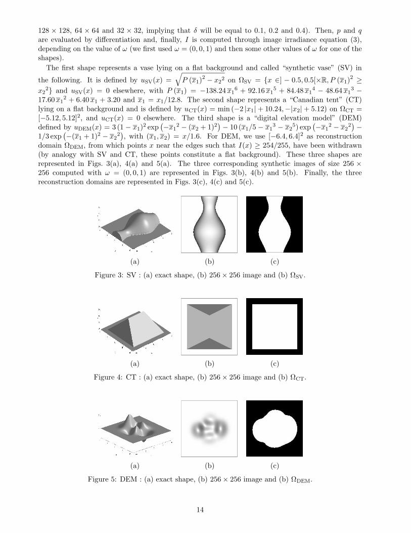
domain ΩDEM, from which points x near the edges such that I(x) ≥ 254/255, have been withdrawn(by analogy with SV and CT, these points constitute a flat background). These three shapes arerepresented in Figs. 3(a), 4(a) and 5(a). The three corresponding synthetic images of size 256 ×256 computed with ω = (0, 0, 1) are represented in Figs. 3(b), 4(b) and 5(b). Finally, the threereconstruction domains are represented in Figs. 3(c), 4(c) and 5(c).

(a) (b) (c)

Figure 3: SV : (a) exact shape, (b) 256× 256 image and (b) ΩSV.

(a) (b) (c)

Figure 4: CT : (a) exact shape, (b) 256× 256 image and (b) ΩCT.

(a) (b) (c)

Figure 5: DEM : (a) exact shape, (b) 256× 256 image and (b) ΩDEM.

14

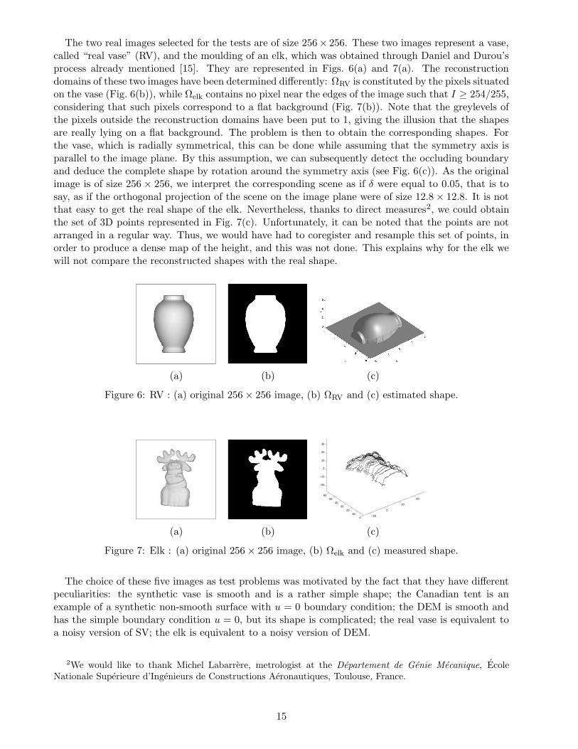
The two real images selected for the tests are of size 256× 256. These two images represent a vase,called “real vase” (RV), and the moulding of an elk, which was obtained through Daniel and Durou’sprocess already mentioned [15]. They are represented in Figs. 6(a) and 7(a). The reconstructiondomains of these two images have been determined differently: ΩRV is constituted by the pixels situatedon the vase (Fig. 6(b)), while Ωelk contains no pixel near the edges of the image such that I ≥ 254/255,considering that such pixels correspond to a flat background (Fig. 7(b)). Note that the greylevels ofthe pixels outside the reconstruction domains have been put to 1, giving the illusion that the shapesare really lying on a flat background. The problem is then to obtain the corresponding shapes. Forthe vase, which is radially symmetrical, this can be done while assuming that the symmetry axis isparallel to the image plane. By this assumption, we can subsequently detect the occluding boundaryand deduce the complete shape by rotation around the symmetry axis (see Fig. 6(c)). As the originalimage is of size 256 × 256, we interpret the corresponding scene as if δ were equal to 0.05, that is tosay, as if the orthogonal projection of the scene on the image plane were of size 12.8× 12.8. It is notthat easy to get the real shape of the elk. Nevertheless, thanks to direct measures2, we could obtainthe set of 3D points represented in Fig. 7(c). Unfortunately, it can be noted that the points are notarranged in a regular way. Thus, we would have had to coregister and resample this set of points, inorder to produce a dense map of the height, and this was not done. This explains why for the elk wewill not compare the reconstructed shapes with the real shape.

(a) (b) (c)

Figure 6: RV : (a) original 256× 256 image, (b) ΩRV and (c) estimated shape.

−20

0

20

40

010

2030

4050

60

−20

−10

0

10

20

30

(a) (b) (c)

Figure 7: Elk : (a) original 256× 256 image, (b) Ωelk and (c) measured shape.

The choice of these five images as test problems was motivated by the fact that they have differentpeculiarities: the synthetic vase is smooth and is a rather simple shape; the Canadian tent is anexample of a synthetic non-smooth surface with u = 0 boundary condition; the DEM is smooth andhas the simple boundary condition u = 0, but its shape is complicated; the real vase is equivalent toa noisy version of SV; the elk is equivalent to a noisy version of DEM.

2We would like to thank Michel Labarrere, metrologist at the Departement de Genie Mecanique, EcoleNationale Superieure d’Ingenieurs de Constructions Aeronautiques, Toulouse, France.

15

3.3 Evaluation of the Performances of the SFS Methods

The most natural criterion for the evaluation of a shape reconstruction is of course to measure thedifference between reconstructed shape u and real shape u. An interesting alternative is to compareinput image I with approximate image I computed from the reconstructed shape, particularly for theelk, the shape of which is not available. Finally, when (p, q) is known for the real shape, it would seeminteresting to compare it with its estimate (p, q) or, even better, to compare normal n to its estimaten, because these two vectors are normed and their comparison is equivalent to the measure of an anglein R

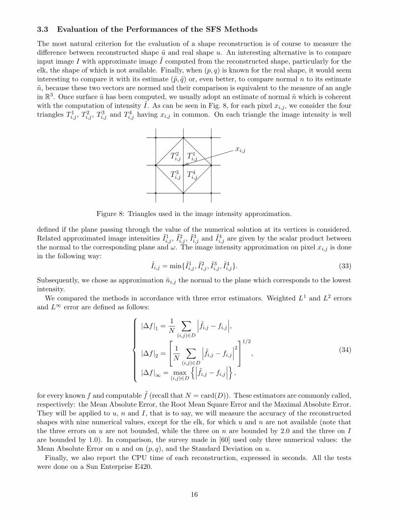
3. Once surface u has been computed, we usually adopt an estimate of normal n which is coherentwith the computation of intensity I. As can be seen in Fig. 8, for each pixel xi,j , we consider the fourtriangles T 1

i,j , T2i,j , T

3i,j and T 4

i,j having xi,j in common. On each triangle the image intensity is well

T 1i,jT 2

i,j

T 4i,jT 3

i,j

xi,j

Figure 8: Triangles used in the image intensity approximation.

defined if the plane passing through the value of the numerical solution at its vertices is considered.Related approximated image intensities I1

i,j , I2i,j , I

3i,j and I4

i,j are given by the scalar product betweenthe normal to the corresponding plane and ω. The image intensity approximation on pixel xi,j is donein the following way:

Ii,j = minI1i,j , I

2i,j , I

3i,j , I

4i,j. (33)

Subsequently, we chose as approximation ni,j the normal to the plane which corresponds to the lowestintensity.

We compared the methods in accordance with three error estimators. Weighted L1 and L2 errorsand L∞ error are defined as follows:

|∆f |1 =1

N

∑

(i,j)∈D

∣∣∣fi,j − fi,j

∣∣∣,

|∆f |2 =

1

N

∑

(i,j)∈D


∣∣∣2

1/2

,

|∆f |∞ = max(i,j)∈D


∣∣∣,

(34)

for every known f and computable f (recall thatN = card(D)). These estimators are commonly called,respectively: the Mean Absolute Error, the Root Mean Square Error and the Maximal Absolute Error.They will be applied to u, n and I, that is to say, we will measure the accuracy of the reconstructedshapes with nine numerical values, except for the elk, for which u and n are not available (note thatthe three errors on u are not bounded, while the three on n are bounded by 2.0 and the three on Iare bounded by 1.0). In comparison, the survey made in [60] used only three numerical values: theMean Absolute Error on u and on (p, q), and the Standard Deviation on u.

Finally, we also report the CPU time of each reconstruction, expressed in seconds. All the testswere done on a Sun Enterprise E420.

16

4 Tests

This section is devoted to the analysis of the tests. At the end of this section we will also discuss therobustness of the algorithms faced with a perturbation in the estimated direction of the light source.

4.1 Test 1: Synthetic Vase

Start from the synthetic image of a vase represented in Fig. 3(b). Two boundary conditions wereconsidered. The first is the homogeneous Dirichlet boundary condition u = 0 in ∂ΩSV which is simple,but clearly false at the top and at the bottom of the vase. The second boundary condition correspondsto u = gSV in ∂ΩSV, where gSV is a continuous function vanishing on the left and on the right handside of the vase, and having the value of the real height at the top and at the bottom. All the errorsfor both choices are provided.

The qualitative behaviour of the surface is well represented in the solutions obtained by the threemethods (Figs. 9, 10 and 11). It can be observed that the TS scheme also gives reasonable informationat the boundary (at the top and at the bottom of the vase); this is surprising because that methodimposes u = 0 as a boundary condition. The effect of boundary conditions is clearly visible in theresults obtained by the FS and DD methods. The FS method does not introduce any smoothing,thus the small kinks on the boundary (which is approximated by square cells) produce several lines ofdiscontinuity for n and for I inside ΩSV. Moreover, the wrong boundary condition u = 0 produces awrong shape due to the concave/convex ambiguity in the model (see Fig. 9(a)). On the other hand,the DD method produces a smooth solution due to the regularization term which is present in thefunctional and does not seem to be affected by the concave/convex ambiguity. The reconstructionof the image after the shape is based on the simple rule I(x) = ω · n(x) and on the methodologydescribed in Section 3. As can be seen in Figs. 12, 13 and 14, the approximation in terms of I is quitesatisfactory for the FS and DD methods. Table 3 shows that all the errors relating to the DD andFS methods have the same order of magnitude in all cases. Note that the results of the TS methodgenerally do not improve by passing from 5 to 20 iterations.

Conversely, Table 1 shows that the DD algorithm is more accurate in the reconstruction of u andis also faster with respect to the FS algorithm (by a factor of 10). Table 2 shows the error in theapproximation of the normals. It can be seen that all the methods have the same order of magnitudeeven if the DD method (on both boundary conditions), and the TS method have lower error testscompared to the FS method.

(a) (b)

Figure 9: FS on SV 256× 256: computed shapes with (a) u = 0 and (b) u = gSV on the boundary.

17

(a) (b)

Figure 10: DD on SV 256× 256: computed shapes with (a) u = 0 and (b) u = gSV on the boundary.

(a) (b)

Figure 11: TS on SV 256× 256: computed shapes with (a) 5 and (b) 20 iterations.

(a) (b)

Figure 12: FS on SV 256× 256: computed images with (a) u = 0 and (b) u = gSV on the boundary.

(a) (b)

Figure 13: DD on SV 256× 256: computed images with (a) u = 0 and (b) u = gSV on the boundary.

18

(a) (b)

Figure 14: TS on SV 256× 256: computed images with (a) 5 and (b) 20 iterations.

Table 1: SV 256× 256: errors on the computed shape and CPU time.

method boundary condition |∆u|1 |∆u|2 |∆u|∞ CPU

FS u = 0 8.2427e-01 1.0171e+00 1.9494e+00 213.0

FS u = gSV 3.0514e-01 3.1881e-01 5.7427e-01 151.4

DD u = 0 6.1508e-01 6.9996e-01 1.9413e+00 15.93

DD u = gSV 1.8528e-01 2.2771e-01 4.3051e-01 16.12

TS (5 it.) u = 0 8.0773e-01 9.6358e-01 1.6910e+00 0.29

TS (20 it.) u = 0 5.0433e-01 6.3173e-01 1.7352e+00 1.17

Table 2: SV 256× 256: errors on the computed normals.

method boundary condition |∆n|1 |∆n|2 |∆n|∞FS u = 0 8.2598e-01 9.2353e-01 1.9802e+00

FS u = gSV 8.6121e-01 9.2691e-01 1.9802e+00

DD u = 0 1.9534e-01 2.8676e-01 1.3111e+00

DD u = gSV 1.1287e-01 1.6782e-01 1.4219e+00

TS (5 it.) u = 0 2.9061e-01 3.3502e-01 1.4190e+00

TS (20 it.) u = 0 2.4689e-01 3.2353e-01 1.4268e+00

19

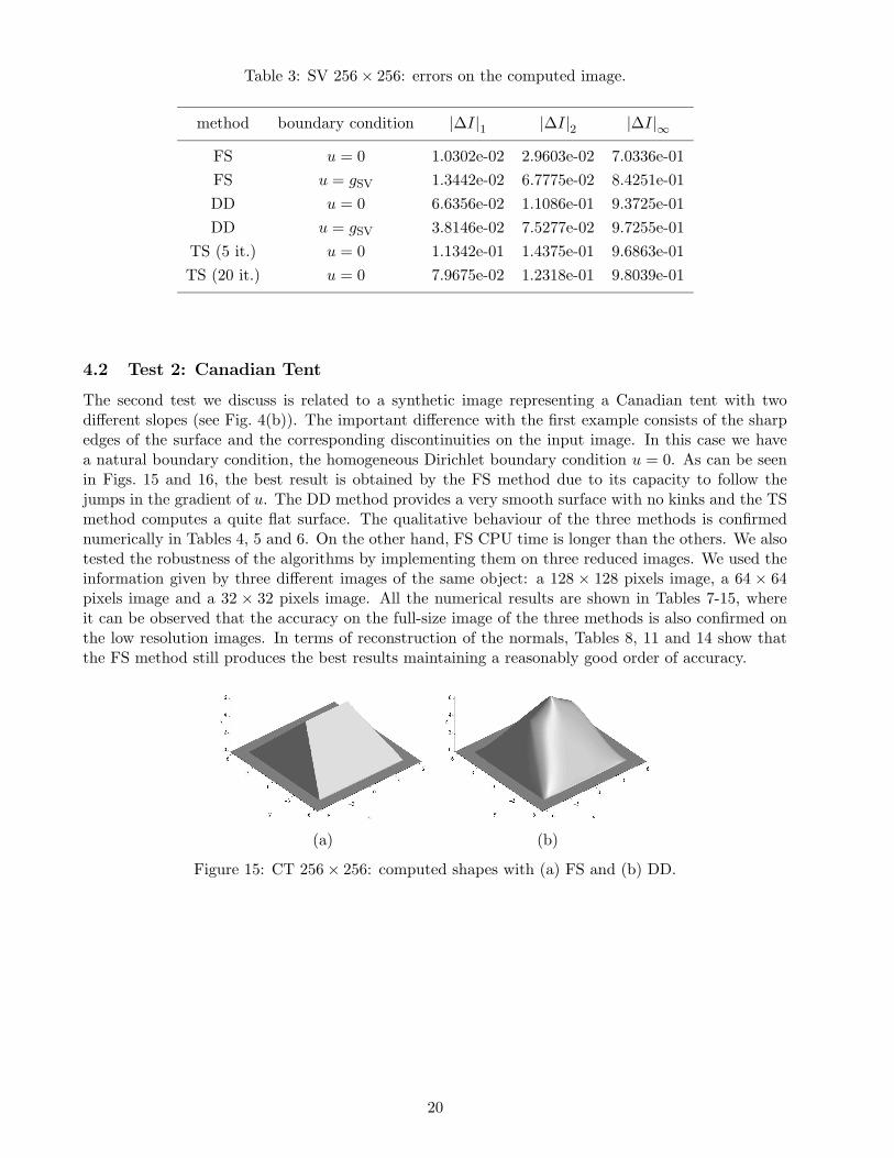
Table 3: SV 256× 256: errors on the computed image.

method boundary condition |∆I|1 |∆I|2 |∆I|∞FS u = 0 1.0302e-02 2.9603e-02 7.0336e-01

FS u = gSV 1.3442e-02 6.7775e-02 8.4251e-01

DD u = 0 6.6356e-02 1.1086e-01 9.3725e-01

DD u = gSV 3.8146e-02 7.5277e-02 9.7255e-01

TS (5 it.) u = 0 1.1342e-01 1.4375e-01 9.6863e-01

TS (20 it.) u = 0 7.9675e-02 1.2318e-01 9.8039e-01

4.2 Test 2: Canadian Tent

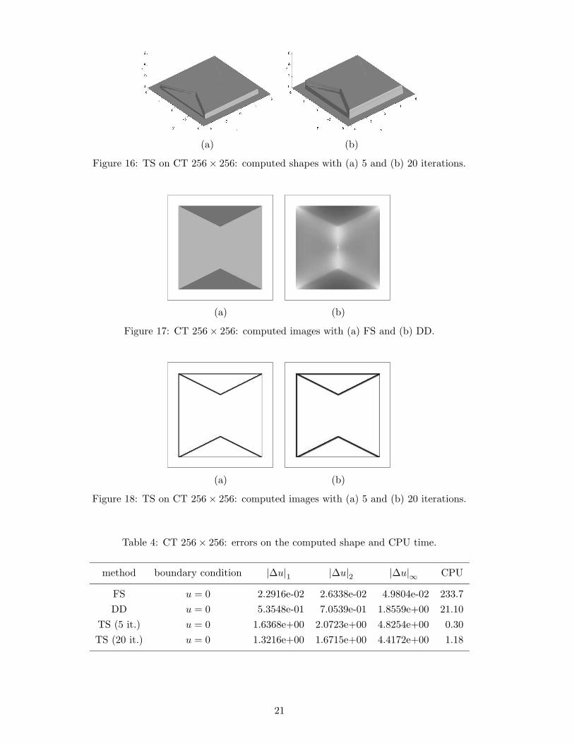
The second test we discuss is related to a synthetic image representing a Canadian tent with twodifferent slopes (see Fig. 4(b)). The important difference with the first example consists of the sharpedges of the surface and the corresponding discontinuities on the input image. In this case we havea natural boundary condition, the homogeneous Dirichlet boundary condition u = 0. As can be seenin Figs. 15 and 16, the best result is obtained by the FS method due to its capacity to follow thejumps in the gradient of u. The DD method provides a very smooth surface with no kinks and the TSmethod computes a quite flat surface. The qualitative behaviour of the three methods is confirmednumerically in Tables 4, 5 and 6. On the other hand, FS CPU time is longer than the others. We alsotested the robustness of the algorithms by implementing them on three reduced images. We used theinformation given by three different images of the same object: a 128 × 128 pixels image, a 64 × 64pixels image and a 32 × 32 pixels image. All the numerical results are shown in Tables 7-15, whereit can be observed that the accuracy on the full-size image of the three methods is also confirmed onthe low resolution images. In terms of reconstruction of the normals, Tables 8, 11 and 14 show thatthe FS method still produces the best results maintaining a reasonably good order of accuracy.

(a) (b)

Figure 15: CT 256× 256: computed shapes with (a) FS and (b) DD.

20

(a) (b)

Figure 16: TS on CT 256× 256: computed shapes with (a) 5 and (b) 20 iterations.

(a) (b)

Figure 17: CT 256× 256: computed images with (a) FS and (b) DD.

(a) (b)

Figure 18: TS on CT 256× 256: computed images with (a) 5 and (b) 20 iterations.

Table 4: CT 256× 256: errors on the computed shape and CPU time.


FS u = 0 2.2916e-02 2.6338e-02 4.9804e-02 233.7

DD u = 0 5.3548e-01 7.0539e-01 1.8559e+00 21.10

TS (5 it.) u = 0 1.6368e+00 2.0723e+00 4.8254e+00 0.30

TS (20 it.) u = 0 1.3216e+00 1.6715e+00 4.4172e+00 1.18

21

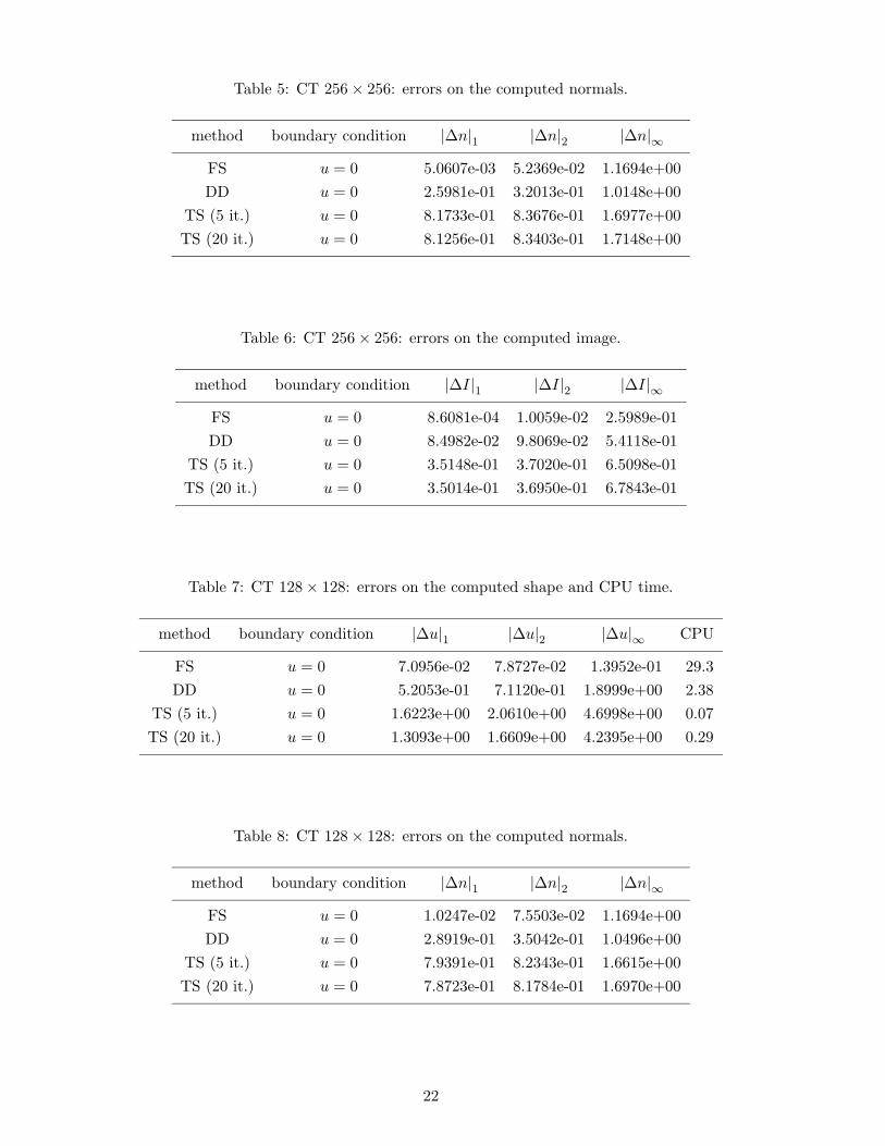
Table 5: CT 256× 256: errors on the computed normals.


DD u = 0 2.5981e-01 3.2013e-01 1.0148e+00

TS (5 it.) u = 0 8.1733e-01 8.3676e-01 1.6977e+00

TS (20 it.) u = 0 8.1256e-01 8.3403e-01 1.7148e+00

Table 6: CT 256× 256: errors on the computed image.


DD u = 0 8.4982e-02 9.8069e-02 5.4118e-01

TS (5 it.) u = 0 3.5148e-01 3.7020e-01 6.5098e-01

TS (20 it.) u = 0 3.5014e-01 3.6950e-01 6.7843e-01



FS u = 0 7.0956e-02 7.8727e-02 1.3952e-01 29.3

DD u = 0 5.2053e-01 7.1120e-01 1.8999e+00 2.38

TS (5 it.) u = 0 1.6223e+00 2.0610e+00 4.6998e+00 0.07

TS (20 it.) u = 0 1.3093e+00 1.6609e+00 4.2395e+00 0.29



DD u = 0 2.8919e-01 3.5042e-01 1.0496e+00

TS (5 it.) u = 0 7.9391e-01 8.2343e-01 1.6615e+00

TS (20 it.) u = 0 7.8723e-01 8.1784e-01 1.6970e+00

22



DD u = 0 8.4821e-02 1.0098e-01 5.3333e-01

TS (5 it.) u = 0 3.3409e-01 3.5641e-01 5.9608e-01

TS (20 it.) u = 0 3.3322e-01 3.5412e-01 6.5098e-01



FS u = 0 4.3838e-02 5.5006e-02 1.1555e-01 3.5

DD u = 0 4.5714e-01 5.9182e-01 1.6306e+00 0.43

TS (5 it.) u = 0 1.6463e+00 2.0819e+00 4.6998e+00 0.02

TS (20 it.) u = 0 1.3158e+00 1.6692e+00 4.2174e+00 0.07



DD u = 0 3.1316e-01 3.8043e-01 1.2770e+0

TS (5 it.) u = 0 7.6224e-01 7.9692e-01 1.5857e+00

TS (20 it.) u = 0 7.3764e-01 7.8453e-01 1.6599e+00



DD u = 0 8.2742e-02 1.0299e-01 5.2157e-01

TS (5 it.) u = 0 3.1088e-01 3.3316e-01 5.5294e-01

TS (20 it.) u = 0 2.9621e-01 3.2371e-01 5.9608e-01

23



FS u = 0 4.1594e-02 5.1906e-02 1.1354e-01 0.4

DD u = 0 5.2870e-01 6.1879e-01 1.4067e+00 0.44

TS (5 it.) u = 0 1.7052e+00 2.1300e+00 4.5383e+00 0.01

TS (20 it.) u = 0 1.3421e+00 1.7021e+00 4.0174e+00 0.02



DD u = 0 3.3752e-01 4.1798e-01 1.3431e+00

TS (5 it.) u = 0 7.2485e-01 7.6012e-01 1.4383e+00

TS (20 it.) u = 0 6.8353e-01 7.3464e-01 1.5826e+00



DD u = 0 8.2974e-02 1.0690e-01 5.0196e-01

TS (5 it.) u = 0 2.9234e-01 3.1537e-01 5.4902e-01

TS (20 it.) u = 0 2.6545e-01 2.8996e-01 5.4902e-01

24

4.3 Test 3: Real Vase

Consider the real image of a vase represented in Fig. 6(a). As in Test 1 (SV) we considered twoboundary conditions. It can be seen from Figs. 19, 20 and 21 and from Tables 16, 17 and 18 that thenumerical results show behaviour in the three methods which is similar to Test 1. It can be noted thatthe DD surface seems to be more accurate in the reconstruction of the shape with respect to FS andTS. However, comparison of the approximate image indicates a better performance of the FS method.Table 17 confirms the DD method to be more accurate in the reconstruction of the normals. Also inthis case CPU times show a big difference between the FS and the DD and TS methods, which arefaster.

(a) (b)

Figure 19: FS on RV 256× 256: computed shapes with (a) u = 0 and (b) u = gRV on the boundary.

(a) (b)

Figure 20: DD on RV 256× 256: computed shapes with (a) u = 0 and (b) u = gRV on the boundary.

(a) (b)

Figure 21: TS on RV 256× 256: computed shapes with (a) 5 and (b) 20 iterations.

25

(a) (b)

Figure 22: FS on RV 256× 256: computed images with (a) u = 0 and (b) u = gRV on the boundary.

(a) (b)

Figure 23: DD on RV 256× 256: computed images with (a) u = 0 and (b) u = gRV on the boundary.

(a) (b)

Figure 24: TS on RV 256× 256: computed images with (a) 5 and (b) 20 iterations.

26

Table 16: RV 256× 256: errors on the computed shape and CPU time.


FS u = 0 7.6917e-01 8.2515e-01 1.7351e+00 111.1

FS u = gRV 5.9975e-01 6.3824e-01 1.0558e+00 97.1

DD u = 0 9.6423e-01 9.9563e-01 1.9027e+00 9.82

DD u = gRV 1.5982e-01 2.3143e-01 5.5699e-01 9.97

TS (5 it.) u = 0 1.2788e+00 1.3721e+00 1.9471e+00 0.30

TS (20 it.) u = 0 4.0640e-01 4.6392e-01 1.2744e+00 1.17

Table 17: RV 256× 256: errors on the computed normals.


FS u = gRV 8.8779e-01 9.4742e-01 1.9548e+00

DD u = 0 2.0691e-01 2.9205e-01 1.1767e+00

DD u = gRV 1.4648e-01 1.9883e-01 1.1624e+00

TS (5 it.) u = 0 3.2854e-01 4.1963e-01 1.8056e+00

TS (20 it.) u = 0 2.5840e-01 3.9742e-01 1.9489e+00

Table 18: RV 256× 256: errors on the computed image.


FS u = gRV 1.4107e-02 5.7083e-02 6.2418e-01

DD u = 0 4.8166e-02 7.7248e-02 6.7843e-01

DD u = gRV 5.3361e-02 8.3276e-02 5.8039e-01

TS (5 it.) u = 0 1.6722e-01 1.8949e-01 7.0980e-01

TS (20 it.) u = 0 1.2244e-01 1.6358e-01 7.8039e-01

27

4.4 Test 4: Digital Elevation Model

This test uses the image of a DEM (see 5(b)). It is first noted that the qualitative behaviour of thereconstructed shapes is very different for the three methods. The FS method computes the maximalsolution, which does not coincide with the real surface, while the DD method computes one of theadmissible minimum energy configurations. Note that the TS shapes reflect a surprising behaviour onthe boundary. In any case, we can observe that the order of magnitude of the errors on the shapesand on the normals is the same for the three methods (see Tables 19 and 20), while Table 21 showsthe different behaviour of the image errors as can also be seen in Figs. 27 and 28. In this test CPUtimes underline the slow behaviour of the FS method.

(a) (b)

Figure 25: DEM 256× 256: computed shapes with (a) FS and (b) DD.

(a) (b)

Figure 26: TS on DEM 256× 256: computed shapes with (a) 5 and (b) 20 iterations.

(a) (b)

Figure 27: DEM 256× 256: computed images with (a) FS and (b) DD.

28

(a) (b)

Figure 28: TS on DEM 256× 256: computed images with (a) 5 and (b) 20 iterations.

Table 19: DEM 256× 256: errors on the computed shape and CPU time.


FS u = 0 4.4378e-01 7.3677e-01 3.3683e+00 508.9

DD u = 0 5.8636e-01 8.8070e-01 2.5147e+00 10.76

TS (5 it.) u = 0 8.4777e-01 9.4934e-01 2.6841e+00 0.30

TS (20 it.) u = 0 1.2647e+00 1.3803e+00 3.3035e+00 1.18

Table 20: DEM 256× 256: errors on the computed normals.


DD u = 0 5.9660e-01 7.0774e-01 1.5120e+00

TS (5 it.) u = 0 6.4650e-01 7.3523e-01 1.4573e+00

TS (20 it.) u = 0 7.4149e-01 8.2825e-01 1.5992e+00

Table 21: DEM 256× 256: errors on the computed image.


DD u = 0 6.0825e-02 8.1257e-02 3.0980e-01

TS (5 it.) u = 0 1.2361e-01 2.2017e-01 9.6078e-01

TS (20 it.) u = 0 1.5492e-01 2.4792e-01 9.7255e-01

29

4.5 Test 5: Elk

This test deals with a real greylevel image representing the plaster of an elk (Fig. 7(a) was kindlyprovided by Daniel, and it has been used in [16] as a test problem). For this image we have noadditional information either for the exact surface or for the normals, so only computed images willbe compared. The pecularity of this example is the complex shape (as well as the complex silhouette).In Table 22, I errors are shown, from which it can be noted that the FS method produces slightlybetter results compared to the DD and TS methods. This is confirmed from computed images shownin Figs. 29 and 30. FS again shows a slow performance, even if CPU times are in this case closer thanthose in other tests.

(a) (b)

Figure 29: Elk 256× 256: computed images with (a) FS and (b) DD.

(a) (b)

Figure 30: TS on elk 256× 256: computed images with (a) 5 and (b) 20 iterations.

Table 22: Elk 256× 256: errors on the computed image and CPU time.

method boundary condition |∆I|1 |∆I|2 |∆I|∞ CPU

FS u = 0 2.1501e-02 3.9609e-02 4.4411e-01 51.3

DD u = 0 1.1754e-01 1.5165e-01 4.9412e-01 9.15

TS (5 it.) u = 0 1.8686e-01 2.4668e-01 7.8431e-01 0.29

TS (20 it.) u = 0 2.4675e-01 3.1291e-01 8.1176e-01 1.19

30

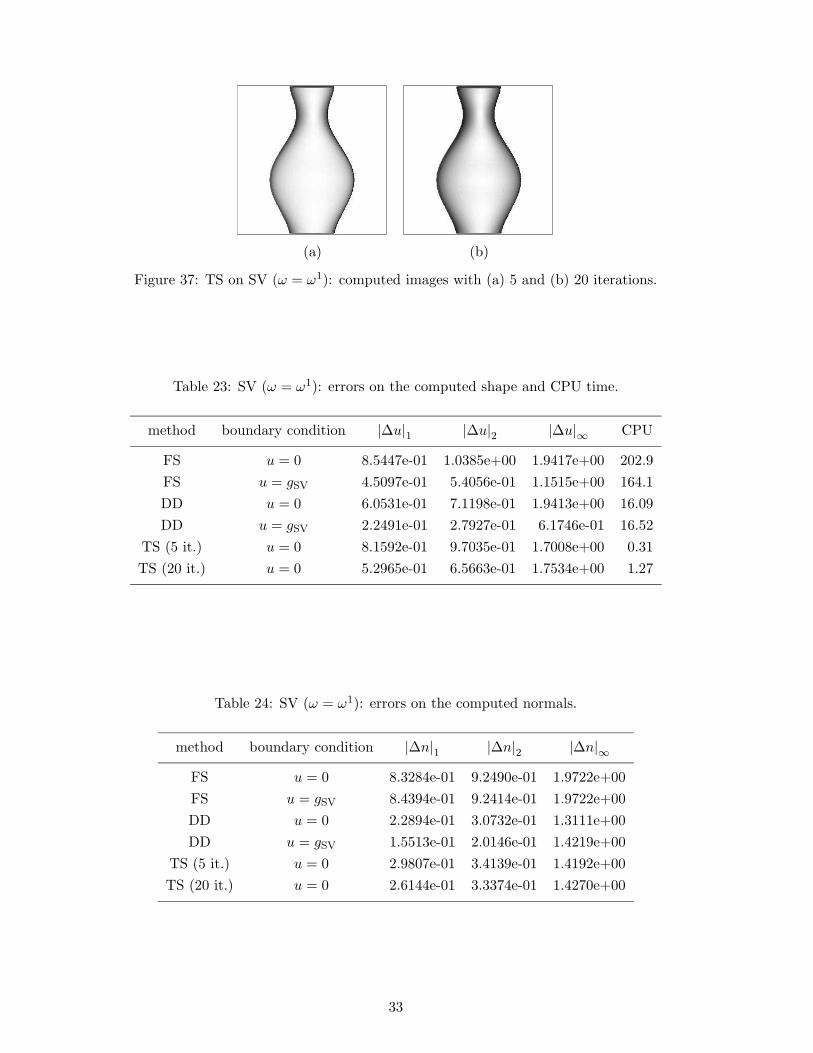
4.6 Test 6: Non-Frontal Lighting

In this last test we wanted to investigate the stability of the three methods with respect to perturba-tions in the light source direction. We considered three images of the synthetic vase that were obtainedusing three different non-frontal light source directions, viz.:

ω1 = (sin(π/36) cos(π/2), sin(π/36) sin(π/2), cos(π/36)),ω2 = (sin(π/18) cos(π/2), sin(π/18) sin(π/2), cos(π/18)),ω3 = (sin(π/18) cos(3π/4), sin(π/18) sin(3π/4), cos(π/18)).

(35)

The three images are represented in Fig. 31. Note that the shadows in the background were not takeninto account, since the background is outside ΩSV. These images were processed as if the light sourcehad been frontal. The two boundary conditions u = 0 (wrong) and u = gSV (right) were considered.Since the numerical results showed that the behaviour of the three methods is similar for the threelight source directions, we limit ourselves to commenting on the Figures and Tables relating to ω1 asa representative example.

The first remark to make is that the order of magnitude of errors on shapes and normals is thesame for all three methods (see Tables 23 and 24) while Table 25 shows some differences in errors onthe computed images. Examining Figs. 32, 33 and 34, it seems that the DD method is reasonablyaccurate, while the FS and TS methods present different problems on the neck and the belly of thevase. However, the qualitative behaviour of the images is well represented in the solution obtained bythe three methods (Figs. 35, 36 and 37). CPU times confirm the better speed of DD and TS comparedto FS.

(a) (b) (c)

Figure 31: SV 256× 256 images: (a) ω = ω1, (b) ω = ω2 and (c) ω = ω3.

(a) (b)

Figure 32: FS on SV (ω = ω1): computed shapes with (a) u = 0 and (b) u = gSV on the boundary.

31

(a) (b)

Figure 33: DD on SV (ω = ω1): computed shapes with (a) u = 0 and (b) u = gSV on the boundary.

(a) (b)

Figure 34: TS on SV (ω = ω1): computed shapes with (a) 5 and (b) 20 iterations.

(a) (b)

Figure 35: FS on SV (ω = ω1): computed images with (a) u = 0 and (b) u = gSV on the boundary.

(a) (b)

Figure 36: DD on SV (ω = ω1): computed images with (a) u = 0 and (b) u = gSV on the boundary.

32

(a) (b)

Figure 37: TS on SV (ω = ω1): computed images with (a) 5 and (b) 20 iterations.

Table 23: SV (ω = ω1): errors on the computed shape and CPU time.


FS u = 0 8.5447e-01 1.0385e+00 1.9417e+00 202.9

FS u = gSV 4.5097e-01 5.4056e-01 1.1515e+00 164.1

DD u = 0 6.0531e-01 7.1198e-01 1.9413e+00 16.09

DD u = gSV 2.2491e-01 2.7927e-01 6.1746e-01 16.52

TS (5 it.) u = 0 8.1592e-01 9.7035e-01 1.7008e+00 0.31

TS (20 it.) u = 0 5.2965e-01 6.5663e-01 1.7534e+00 1.27

Table 24: SV (ω = ω1): errors on the computed normals.


FS u = gSV 8.4394e-01 9.2414e-01 1.9722e+00

DD u = 0 2.2894e-01 3.0732e-01 1.3111e+00

DD u = gSV 1.5513e-01 2.0146e-01 1.4219e+00

TS (5 it.) u = 0 2.9807e-01 3.4139e-01 1.4192e+00

TS (20 it.) u = 0 2.6144e-01 3.3374e-01 1.4270e+00

33

Table 25: SV (ω = ω1): errors on the computed image.


FS u = gSV 1.5390e-02 7.7637e-02 9.1307e-01

DD u = 0 7.4405e-02 1.1557e-01 9.8431e-01

DD u = gSV 4.9549e-02 8.3209e-02 9.7255e-01

TS (5 it.) u = 0 1.1799e-01 1.4993e-01 9.6863e-01

TS (20 it.) u = 0 8.2467e-02 1.2607e-01 9.8039e-01

5 Conclusion

We finish the paper by drawing some conclusions based on the analyses and numerical tests presentedin the previous sections.

As far as the mathematical properties of the three methods is concerned, we note that the FS andDD methods always converge to a solution of the SFS problem, whereas convergence is not guaranteedby the TS method. As can be seen by the tests in Section 4, it is not simply a question of style. Infact, increasing the number of iterations in TS often does not improve the solution in terms of anyof our error indicators. However, it should be noted that the DD algorithm converges in general to alocal minimum, and the search for a global minimum would require much more computational effort.The FS method converges to the maximal solution which, in general, will not coincide with the realsurface.

The minimization method suggested by Daniel and Durou seems to produce accurate results forsmooth surfaces, and the Dirichlet boundary conditions are easily included in the algorithm. Themethod put forward by Tsai and Shah gives its best results on smooth surfaces but suffers in somecases, particularly when the surface have several maxima and minima (as in Test 4). Moreover, itseems impossible to change the Dirichlet boundary condition in that method. Finally, Falcone andSagona’s method seems to be well adapted to a variety of different situations which include smoothand non-smooth surfaces and can cope with Dirichlet boundary conditions. However, its weak pointseems to be CPU time and the absence of smooting in the surfaces which in some cases producedlarger errors in the reconstruction of the normals.

The three methods appear to be stable in presence of a perturbation in the light source direc-tion. They all compute a reasonable solution although FS seems to be more sensitive to this kind ofperturbation.

The analyses contained in this paper could give rise to several interesting developments and im-provements. The first improvement is related to the use of fast marching methods for the solutionof the eikonal equation to reduce CPU time in the FS method. As far as the minimization methodsare concerned, it would be desirable to reduce the regularization term in order to keep the corners ofthe shapes. For all the methods, it would be interesting to deal with “black shadows” (generated byan oblique light source) avoiding additional conditions on the boundaries separating light and shadowregions. We hope to return to these problems in our future research.

34

Acknowledgments

This work was partially supported by the MURST Funds “Scientific Computing” and by the TMR Net-work “Viscosity Solutions and Applications” (contract FMRX-CT98-0234). We thank Alain Crouzilfor his help with the manuscript, which was given its final form by James Munnick of the Centre de

Traduction, Universite Paul Sabatier, Toulouse, France.

References

[1] M. Bardi and M. Falcone. An Approximation Scheme for the Minimum Time Function. SIAM

Journal of Control and Optimization, 28(4):950–965, July 1990.

[2] M. Bardi and M. Falcone. Discrete Approximation of the Minimal Time Function for Systemswith Regular Optimal Trajectories. In A. Bensoussan and P.-L. Lions, editors, Analysis and

Optimization of Systems, volume 144 of Lecture Notes in Control and Information Sciences,pages 103–112. Springer-Verlag, 1990.

[3] G. Barles. Solutions de viscosite des equations de Hamilton-Jacobi. Springer-Verlag, 1994.

[4] A. Blake, A. Zisserman, and G. Knowles. Surface Descriptions from Stereo and Shading. Image

and Vision Computing, 3(4):183–191, 1985.

[5] J.-F. Bonnans, J.-C. Gilbert, C. Lemarechal, and C. A. Sagastizabal, editors. Numerical Opti-

mization: Theoretical and Practical Aspects. Springer-Verlag, 2002.

[6] A. R. Bruss. The Eikonal Equation: Some Results Applicable to Computer Vision. Journal of

Mathematical Physics, 23(5):890–896, May 1982.

[7] F. Camilli and M. Falcone. An Approximation Scheme for the Maximal Solution of the Shape-from-Shading Problem. In Proceedings of the 3rd International Conference on Image Processing,volume I, pages 49–52, Lausanne, Switzerland, September 1996.

[8] F. Camilli and L. Grune. Numerical Approximation of the Maximal Solutions for a Class ofDegenerate Hamilton-Jacobi Equations. SIAM Journal on Numerical Analysis, 38(5):1540–1560,2000.

[9] F. Camilli and A. Siconolfi. Discontinuous Solutions of a Hamilton-Jacobi Equation with InfiniteSpeed of Propagation. SIAM Journal on Mathematical Analysis, 28(6):1420–1445, 1997.

[10] F. Camilli and A. Siconolfi. Maximal Subsolutions of a Class of Degenerate Hamilton-JacobiProblems. Indiana University Mathematics Journal, 48:1111–1131, 1999.

[11] M. G. Crandall, H. Ishii, and P.-L. Lions. User’s Guide to Viscosity Solutions of Second OrderPartial Differential Equations. Bulletin of the American Mathematical Society, 27(1):1–67, July1992.

[12] M. G. Crandall and P.-L. Lions. Two Approximations of Solutions of Hamilton-Jacobi Equations.Mathematics of Computation, 43(167):1–19, 1984.

[13] A. Crouzil, X. Descombes, and J.-D. Durou. A Multiresolution Approach for Shape from ShadingCoupling Deterministic and Stochastic Optimization. IEEE Transactions on Pattern Analysis and

Machine Intelligence, 25(11):1416–1421, November 2003.

[14] P. Daniel. Peut-on extraire le relief d’une seule image ? These de doctorat, Universite PaulSabatier, Toulouse, France, January 2000. (in French).

35

[15] P. Daniel and J.-D. Durou. Creation of Real Images which are Valid for the Assumptions Madein Shape From Shading. In Proceedings of the 10th International Conference on Image Analysis

and Processing, pages 418–423, Venice, Italy, September 1999.

[16] P. Daniel and J.-D. Durou. From Deterministic to Stochastic Methods for Shape From Shading.In Proceedings of the 4th Asian Conference on Computer Vision, pages 187–192, Taipei, Taiwan,January 2000.

[17] J.-D. Durou and H. Maıtre. On Convergence in the Methods of Strat and of Smith for Shapefrom Shading. International Journal of Computer Vision, 17(3):273–289, March 1996.

[18] J.-D. Durou and D. Piau. Ambiguous Shape from Shading with Critical Points. Journal of

Mathematical Imaging and Vision, 12(2):99–108, April 2000.

[19] M. Falcone, T. Giorgi, and P. Loreti. Level Sets of Viscosity Solutions: Some Applications toFronts and Rendez-Vous Problems. SIAM Journal of Applied Mathematics, 54(5):1335–1354,October 1994.

[20] M. Falcone and M. Sagona. An Algorithm for the Global Solution of the Shape-from-ShadingModel. In Proceedings of the 9th International Conference on Image Analysis and Processing,volume I, pages 596–603, Florence, Italy, September 1997.

[21] R. T. Frankot and R. Chellappa. A Method for Enforcing Integrability in Shape from ShadingAlgorithms. IEEE Transactions on Pattern Analysis and Machine Intelligence, 10(4):439–451,July 1988.

[22] H. B. Griffiths. Surfaces. Cambridge University Press, 1981.

[23] H. Hayakawa, S. Nishida, Y. Wada, and M. Kawato. A Computational Model for Shape Estima-tion by Integration of Shading and Edge Information. Neural Networks, 7(8):1193–1209, October1994.

[24] B. K. P. Horn. Obtaining Shape from Shading Information. In P. H. Winston, editor, The

Psychology of Computer Vision, chapter 4, pages 115–155. McGraw-Hill, 1975.

[25] B. K. P. Horn. Height and Gradient from Shading. International Journal of Computer Vision,5(1):37–75, August 1990.

[26] B. K. P. Horn and M. J. Brooks. The Variational Approach to Shape From Shading. Computer

Vision, Graphics, and Image Processing, 33(2):174–208, February 1986.

[27] B. K. P. Horn and M. J. Brooks, editors. Shape from Shading. MIT Press, 1989.

[28] B. K. P. Horn, R. Szeliski, and A. L. Yuille. Impossible Shaded Images. IEEE Transactions on

Pattern Analysis and Machine Intelligence, 15(2):166–170, February 1993.

[29] K. Ikeuchi and B. K. P. Horn. Numerical Shape from Shading and Occluding Boundaries. Artificial

Intelligence, 17(1–3):141–184, August 1981.

[30] H. Ishii and M. Ramaswamy. Uniqueness Results for a Class of Hamilton-Jacobi Equations withSingular Coefficients. Communications in Partial Differential Equations, 20:2187–2213, 1995.

[31] R. Kimmel and A. M. Bruckstein. Tracking Level Sets by Level Sets: A Method for Solving theShape from Shading Problem. Center for Intelligent System Report CIS9319, Technion-IsraelInstitute of Technology, Haifa, Israel, May 1993.

36

[32] R. Kimmel and A. M. Bruckstein. Global Shape from Shading. In Proceedings of the 12th

International Conference on Pattern Recognition, volume I, pages 120–125, Jerusalem, Israel,October 1994.

[33] R. Kimmel and J. A. Sethian. Optimal Algorithm for Shape from Shading and Path Planning.Journal of Mathematical Imaging and Vision, 14(3):237–244, May 2001.

[34] R. Kozera. A Note on Existence and Uniqueness in Shape from Shading. In Proceedings of the

4th IEEE International Conference on Computer Vision, pages 507–511, Berlin, Germany, May1993.

[35] R. Kozera and R. Klette. Finite Difference Based Algorithms in Linear Shape from Shading.Machine Graphics and Vision, 6(2):157–201, 1997.

[36] Y. G. Leclerc and A. F. Bobick. The Direct Computation of Height from Shading. In Proceedings

of the IEEE Conference on Computer Vision and Pattern Recognition, pages 552–558, Maui,Hawaii, USA, June 1991.

[37] D. Lee. A Provably Convergent Algorithm for Shape from Shading. In Proceedings of the Image

Understanding Workshop, pages 489–496, Miami Beach, Florida, USA, December 1985.

[38] K. M. Lee and C.-C. J. Kuo. Shape from Shading with a Linear Triangular Element SurfaceModel. IEEE Transactions on Pattern Analysis and Machine Intelligence, 15(8):815–822, August1993.

[39] P.-L. Lions. Generalized Solutions of Hamilton-Jacobi Equations. Pitman, 1982.

[40] P.-L. Lions, E. Rouy, and A. Tourin. Shape-from-Shading, Viscosity Solutions and Edges. Nu-

merische Mathematik, 64:323–353, 1993.

[41] J. Malik and D. Maydan. Recovering Three-Dimensional Shape from a Single Image of CurvedObjects. IEEE Transactions on Pattern Analysis and Machine Intelligence, 11(6):555–566, June1989.

[42] J. Oliensis. Uniqueness in Shape from Shading. International Journal of Computer Vision,6(2):75–104, June 1991.

[43] J. Oliensis and P. Dupuis. A Global Algorithm for Shape from Shading. In Proceedings of the

4th IEEE International Conference on Computer Vision, pages 692–701, Berlin, Germany, May1993.

[44] S. J. Osher and J. A. Sethian. Fronts Propagating with Curvature-Dependent Speed: AlgorithmsBased on Hamilton-Jacobi Formulations. Journal of Computational Physics, 79(1):12–49, 1988.

[45] A. P. Pentland. Local Shading Analysis. IEEE Transactions on Pattern Analysis and Machine

Intelligence, 6(2):170–187, March 1984.

[46] A. P. Pentland. Linear Shape from Shading. International Journal of Computer Vision, 4(2):153–162, March 1990.

[47] E. Prados, O. Faugeras, and E. Rouy. Shape from Shading and Viscosity Solutions. In Proceedings

of the 7th European Conference on Computer Vision, volume II, pages 790–804, Copenhagen,Denmark, May 2002.

[48] T. Rindfleisch. Photometric Method for Lunar Topography. Photometric Engineering, 32(2):262–277, March 1966.

37

[49] E. Rouy and A. Tourin. A Viscosity Solutions Approach to Shape from Shading. SIAM Journal

on Numerical Analysis, 29(3):867–884, June 1992.

[50] M. Sagona. Numerical methods for degenerate Eikonal type equations and applications. Tesidi dottorato, Dipartimento di Matematica dell’Universita di Napoli “Federico II”, Napoli, Italy,November 2001.

[51] J. A. Sethian and A. Vladimirsky. Fast Methods for the Eikonal and Related Hamilton-JacobiEquations on Unstructured Meshes. Proceedings of the National Academy of Sciences of the USA,97(11):5699–5703, 2000.

[52] T. M. Strat. A Numerical Method for Shape from Shading from a Single Image. Master’sthesis, Department of Electrical Engineering and Computer Science, Massachusetts Institute ofTechnology, Cambridge, Massachusetts, USA, 1979.

[53] R. Szeliski. Fast Shape from Shading. Computer Vision, Graphics, and Image Processing: Image

Understanding, 53(2):129–153, March 1991.

[54] P.-S. Tsai and M. Shah. Shape from Shading Using Linear Approximation. Image and Vision

Computing, 12(8):487–498, October 1994.

[55] G. Ulich. Provably Convergent Methods for the Linear and Nonlinear Shape from Shading Prob-lem. Journal of Mathematical Imaging and Vision, 9(1):69–82, July 1998.

[56] J. Van Diggelen. A Photometric Investigation of the Slopes and Heights of the Ranges of Hills inthe Maria of the Moon. Bulletin of the Astronomical Institute of the Netherlands, 11(423):283–290, July 1951.

[57] R. L. Wildey. Radarclinometry for the Venus Radar Mapper. Photogrammetric Engineering and

Remote Sensing, 52(1):41–50, January 1986.

[58] P. L. Worthington and E. R. Hancock. New Constraints on Data-Closeness and Needle MapConsistency for Shape-from-Shading. IEEE Transactions on Pattern Analysis and Machine In-

telligence, 21(12):1250–1267, December 1999.

[59] Z. Wu and L. Li. A Line-Integration Based Method for Depth Recovery from Surface Normals.Computer Vision, Graphics, and Image Processing, 43(1):53–66, July 1988.

[60] R. Zhang, P.-S. Tsai, J. E. Cryer, and M. Shah. Shape from Shading: A Survey. IEEE Transac-

tions on Pattern Analysis and Machine Intelligence, 21(8):690–706, August 1999.

38

a survey of numerical methods for shape from...

Documents