a survey of wheel/rail friction - transportation
TRANSCRIPT
U.S. Department of Transportation
Federal Railroad Administration
A Survey of Wheel/Rail Friction
Office of Research, Development and Technology Washington, DC 20590
DOT/FRA/ORD-17-21 Final Report September 2017
NOTICE
This document is disseminated under the sponsorship of the Department of Transportation in the interest of information exchange. The United States Government assumes no liability for its contents or use thereof. Any opinions, findings and conclusions, or recommendations expressed in this material do not necessarily reflect the views or policies of the United States Government, nor does mention of trade names, commercial products, or organizations imply endorsement by the United States Government. The United States Government assumes no liability for the content or use of the material contained in this document.
NOTICE
The United States Government does not endorse products or manufacturers. Trade or manufacturers’ names appear herein solely because they are considered essential to the objective of this report.
i
REPORT DOCUMENTATION PAGE Form Approved OMB No. 0704-0188
Public reporting burden for this collection of information is estimated to average 1 hour per response, including the time for reviewing instructions, searching existing data sources, gathering and maintaining the data needed, and completing and reviewing the collection of information. Send comments regarding this burden estimate or any other aspect of this collection of information, including suggestions for reducing this burden, to Washington Headquarters Services, Directorate for Information Operations and Reports, 1215 Jefferson Davis Highway, Suite 1204, Arlington, VA 22202-4302, and to the Office of Management and Budget, Paperwork Reduction Project (0704-0188), Washington, DC 20503.
1. AGENCY USE ONLY (Leave blank)
2. REPORT DATE September 2017
3. REPORT TYPE AND DATES COVERED Technical Report
4. TITLE AND SUBTITLE A Survey of Wheel/Rail Friction
5. FUNDING NUMBERS
6. AUTHOR(S) Eric E. Magel
7. PERFORMING ORGANIZATION NAME(S) AND ADDRESS(ES) National Research Council, Canada 2320 Lester Road, Ottawa, Ontario, Canada K1V 1S2
8. PERFORMING ORGANIZATION REPORT NUMBER
9. SPONSORING/MONITORING AGENCY NAME(S) AND ADDRESS(ES) U.S. Department of Transportation Federal Railroad Administration Office of Research, Development and Technology Washington, DC 20590
10. SPONSORING/MONITORING AGENCY REPORT NUMBER
DOT/FRA/ORD-17/21
11. SUPPLEMENTARY NOTES COR: Ali Tajaddini 12a. DISTRIBUTION/AVAILABILITY STATEMENT This document is available to the public through the FRA Web site at http://www.fra.dot.gov.
12b. DISTRIBUTION CODE
13. ABSTRACT (Maximum 200 words) Friction has a huge influence on the vehicle/track interaction and yet it remains poorly understood, its consideration an afterthought in many simulation activities. This survey of friction summarizes current understanding and identifies gaps requiring further development. Classical friction theory and modern approaches to modelling are reviewed, and lubrication and friction management practices are discussed. Methods for measuring friction at the wheel/rail contact, in both small and full scale systems, are documented. 14. SUBJECT TERMS Friction, friction management, lubrication, vehicle-track interaction, wheel-rail interaction
15. NUMBER OF PAGES 89
16. PRICE CODE
17. SECURITY CLASSIFICATION OF REPORT Unclassified
18. SECURITY CLASSIFICATION OF THIS PAGE Unclassified
19. SECURITY CLASSIFICATION OF ABSTRACT Unclassified
20. LIMITATION OF ABSTRACT
NSN 7540-01-280-5500 Standard Form 298 (Rev. 2-89) Prescribed by ANSI Std. 239-18
298-102
ii
METRIC/ENGLISH CONVERSION FACTORS
ENGLISH TO METRIC METRIC TO ENGLISH
LENGTH (APPROXIMATE) LENGTH (APPROXIMATE) 1 inch (in) = 2.5 centimeters (cm) 1 millimeter (mm) = 0.04 inch (in) 1 foot (ft) = 30 centimeters (cm) 1 centimeter (cm) = 0.4 inch (in)
1 yard (yd) = 0.9 meter (m) 1 meter (m) = 3.3 feet (ft) 1 mile (mi) = 1.6 kilometers (km) 1 meter (m) = 1.1 yards (yd)
1 kilometer (km) = 0.6 mile (mi)
AREA (APPROXIMATE) AREA (APPROXIMATE) 1 square inch (sq in, in2) = 6.5 square centimeters (cm2) 1 square centimeter (cm2) = 0.16 square inch (sq in, in2)
1 square foot (sq ft, ft2) = 0.09 square meter (m2) 1 square meter (m2) = 1.2 square yards (sq yd, yd2) 1 square yard (sq yd, yd2) = 0.8 square meter (m2) 1 square kilometer (km2) = 0.4 square mile (sq mi, mi2) 1 square mile (sq mi, mi2) = 2.6 square kilometers (km2) 10,000 square meters (m2) = 1 hectare (ha) = 2.5 acres
1 acre = 0.4 hectare (he) = 4,000 square meters (m2)
MASS - WEIGHT (APPROXIMATE) MASS - WEIGHT (APPROXIMATE) 1 ounce (oz) = 28 grams (gm) 1 gram (gm) = 0.036 ounce (oz) 1 pound (lb) = 0.45 kilogram (kg) 1 kilogram (kg) = 2.2 pounds (lb)
1 short ton = 2,000 pounds (lb)
= 0.9 tonne (t) 1 tonne (t)
= =
1,000 kilograms (kg) 1.1 short tons
VOLUME (APPROXIMATE) VOLUME (APPROXIMATE) 1 teaspoon (tsp) = 5 milliliters (ml) 1 milliliter (ml) = 0.03 fluid ounce (fl oz)
1 tablespoon (tbsp) = 15 milliliters (ml) 1 liter (l) = 2.1 pints (pt) 1 fluid ounce (fl oz) = 30 milliliters (ml) 1 liter (l) = 1.06 quarts (qt)
1 cup (c) = 0.24 liter (l) 1 liter (l) = 0.26 gallon (gal) 1 pint (pt) = 0.47 liter (l)
1 quart (qt) = 0.96 liter (l) 1 gallon (gal) = 3.8 liters (l)
1 cubic foot (cu ft, ft3) = 0.03 cubic meter (m3) 1 cubic meter (m3) = 36 cubic feet (cu ft, ft3) 1 cubic yard (cu yd, yd3) = 0.76 cubic meter (m3) 1 cubic meter (m3) = 1.3 cubic yards (cu yd, yd3)
TEMPERATURE (EXACT) TEMPERATURE (EXACT)
[(x-32)(5/9)] °F = y °C [(9/5) y + 32] °C = x °F
QUICK INCH - CENTIMETER LENGTH CONVERSION10 2 3 4 5
InchesCentimeters 0 1 3 4 52 6 1110987 1312
QUICK FAHRENHEIT - CELSIUS TEMPERATURE CONVERSIO -40° -22° -4° 14° 32° 50° 68° 86° 104° 122° 140° 158° 176° 194° 212°
°F
°C -40° -30° -20° -10° 0° 10° 20° 30° 40° 50° 60° 70° 80° 90° 100°
For more exact and or other conversion factors, see NIST Miscellaneous Publication 286, Units of Weights and Measures. Price $2.50 SD Catalog No. C13 10286 Updated 6/17/98
iii
Contents
Executive Summary ........................................................................................................................ 9
1. Introduction ............................................................................................................... 11 1.1 Traction and braking ................................................................................................. 11 1.2 Curving ...................................................................................................................... 12
2. What is Friction? ....................................................................................................... 14 2.1 Classical Theory ........................................................................................................ 14 2.2 Influence of Contaminants ........................................................................................ 15 2.3 The Third Body Layer (3BL) .................................................................................... 16 2.4 The Traction-Creepage Characteristic ....................................................................... 22 2.5 The Friction Circle .................................................................................................... 26 2.6 The influence of surface roughness ........................................................................... 27 2.7 The Influence of speed .............................................................................................. 29 2.8 Influence of Normal Load (Contact Stress) .............................................................. 33 2.9 The Influence of Humidity ........................................................................................ 34 2.10 The Influence of Water .............................................................................................. 36 2.11 The Influence of Temperature ................................................................................... 37
3. Friction Modeling ...................................................................................................... 39 3.1 Velocity Accommodation .......................................................................................... 39 3.2 The Percent Kalker (%KALKER) Approach ............................................................ 41 3.3 Other Approaches to Modelling Friction .................................................................. 44 3.4 Friction Modelling - An International Collaborative Research Project .................... 44
4. Friction Control ......................................................................................................... 46 4.1 (Gage-face/Wheel-flange) Lubrication ..................................................................... 47 4.2 Friction Modification (Top of Rail or Wheel Tread) ................................................ 50
5. Methods for Measuring Friction ................................................................................ 60 5.1 Laboratory-Scale Systems ......................................................................................... 60 5.2 Field Measuring Systems .......................................................................................... 65
6. Conclusion ................................................................................................................. 75 6.1 Instrumentation .......................................................................................................... 75 6.2 Gage-face/Wheel-flange ............................................................................................ 75 6.3 Modeling ................................................................................................................... 76 6.4 Testing ....................................................................................................................... 76 6.5 Products ..................................................................................................................... 76
7. References ................................................................................................................. 78
Abbreviations and Acronyms ....................................................................................................... 83
Definitions and Terminology ........................................................................................................ 84
iv
Illustrations
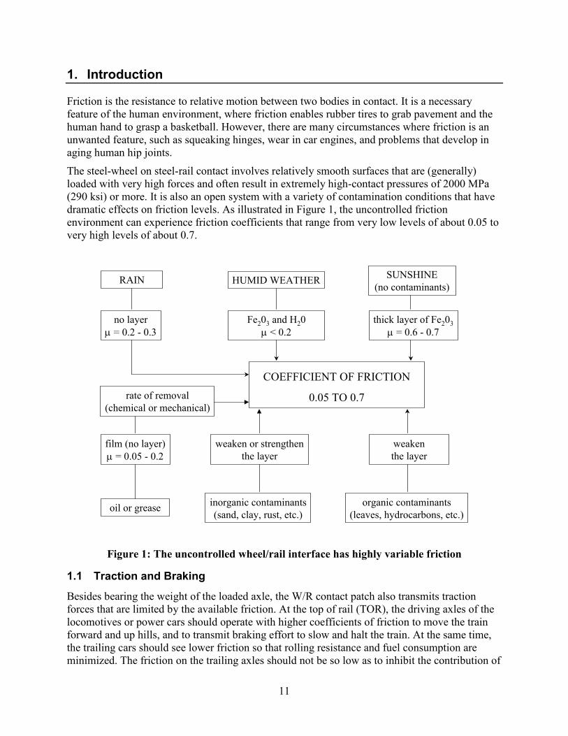
Figure 1: The uncontrolled wheel/rail interface has highly variable friction ............................... 11
Figure 2: In the unlubricated case, wear of the rail gage-face (and wheel flange) can be severe, with wear particles piling up around the rail fasteners ......................................................... 12
Figure 3: Relative motion of two rough surfaces will require deformation of contacting asperities [Fig. 4-4 of Ref. 4]. ............................................................................................................... 14
Figure 4: Friction coefficient for different levels of contamination (cuncontaminated=1) and shear strength ratio (α≃PY
2/SY2) ..................................................................................................... 16
Figure 5: Well defined oxide layers: A) dried on the wheel tread after stopping in a yard and B) during light rain a slurry forms on the rail ............................................................................ 17
Figure 6: The bathtub model illustrates the various inputs (sources) and outputs (sinks) and processes occuring within the layer that affect its composition. .......................................... 18
Figure 7: Even on dry surfaces, layers of iron oxide separate the wheel and rail. The thickness of the layer can be judged by scratching to reveal the bare metal and then focusing on the two surfaces with a microscope. .................................................................................................. 18
Figure 8: Analysis of the 3BL in France found that it is composed of non-oxidized wheel/rail particles and some other contaminants [11].......................................................................... 19
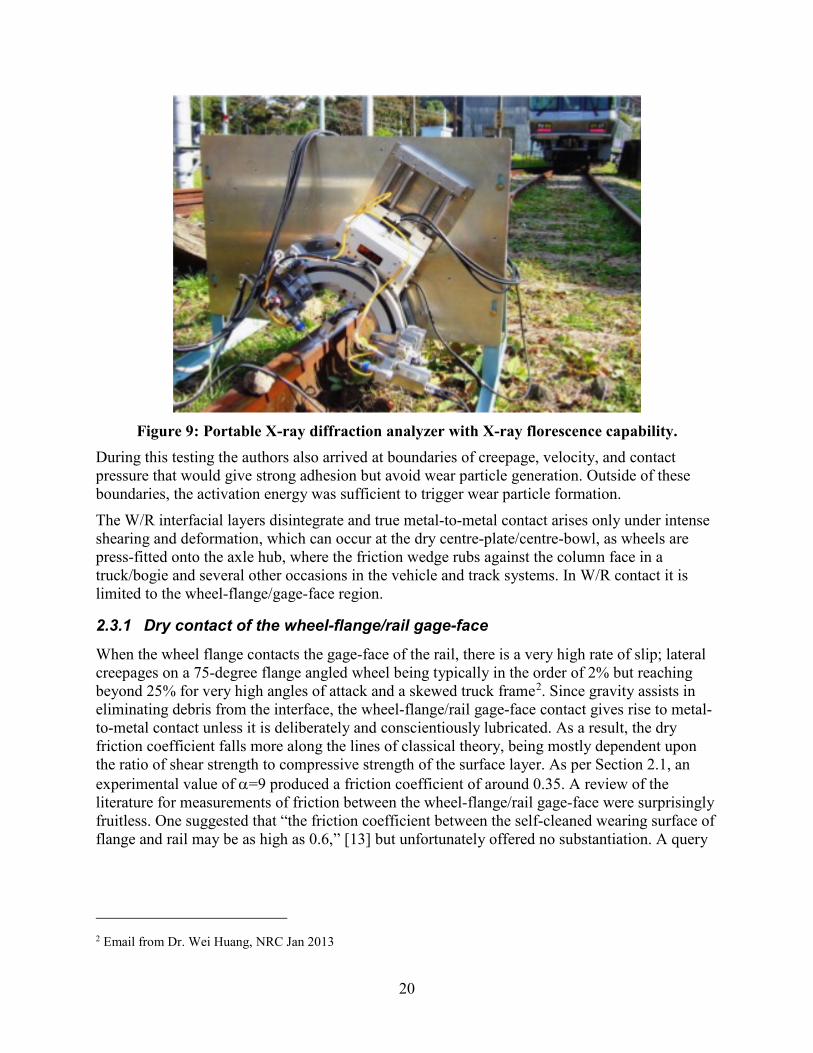
Figure 9: Portable X-ray diffraction analyzer with X-ray florescence capability. ....................... 20
Figure 10: Examples of leaf-fall contamination on the railhead. .................................................. 21
Figure 11: Two elements in contact at the entrance to the contact zone are some distance apart after traversing through the contact under a driving traction. ............................................... 22
Figure 12: Kalker's theoretical curve is affected significantly by the presence of interfacial contaminants [19].................................................................................................................. 23
Figure 13: Traction-creep curves encountered in practice tend to have a negative friction slope beyond saturation. ................................................................................................................. 24
Figure 14: A mechanical system to illustrate stick slip. ............................................................... 25
Figure 15: Shear stress curves for several compounds. ................................................................ 25
Figure 16: The friction circle illustrates that the vectorial sum of the lateral (L) and longitudinal (N) creepage components is confined to the traction limit T. ............................................... 26
Figure 17: Lubrication in curves can lead to a dramatic increase in the lateral forces (RED line) compared with the unlubricated case (BLACK line). ........................................................... 27
Figure 18: Contact between the freshly trued wheel and worn rail is strongly influenced by the rough surface geometry [28]. ................................................................................................ 28
Figure 19: Surface profiles on three different facets of a freshly ground rail surface (top) and after 3 days (<0.1 MGT) of traffic (bottom) on a light axle load LRT system in California [Fig. 8 from Ref. 32]. ............................................................................................................ 29
v
Figure 20: Adhesion-creepage curves for different values of rolling velocity [11] using a unique disc-on-rail test rig. g refers to the applied creepage. ........................................................... 30
Figure 21: Increasing speed is accompanied by a drop in measured friction this series of tests on a small scale 2 disc rig [33]. .................................................................................................. 30
Figure 22: Adhesion as a function of speed under dry conditions with a rail-roller rig [34]. ...... 31
Figure 23: A) Adhesion coefficient measured on UK railways [36]. B) Design adhesion-traction characteristic for high speed trains, based on roller rig testing [35]. The design curve matches closely to the Dry Rail (UIC) measurements. ......................................................... 32
Figure 24: Effect of speed on the traction creepage characteristic [40]. ...................................... 32
Figure 25: The impact of normal contact stress on traction levels at low coefficient of friction in one case (A) increases for this rig that controls longitudinal creepage and to decrease for another (B) that measures friction with lateral creepage. ..................................................... 33
Figure 26: Adhesion-creepage curves for different values of maximum Hertzian pressure [11]. 34
Figure 27: The influence of humidity on adhesion: top-left) using the Sheffield friction pendulum [43], top-right) from Beagley [13], bottom) from Broster et al [10]. ................................... 35
Figure 28: Twin disc testing to assess the impact of relative humidity (Figure 9 of Ref. 42). ..... 36
Figure 29: Humidity was found to have a relatively small effect on friction when leaves are present [15]. .......................................................................................................................... 36
Figure 30: On the basis of strength properties decreasing as temperature rises (left plot), the coefficient of friction (right plot) is assumed to decrease in step [48]. ................................ 38
Figure 31: Effect of temperature on traction coefficient, using a two-disc test rig [42]. .............. 38
Figure 32: Velocity accommodation mechanism – 4 modes x 5 sites = 20 mechanisms. ............ 39
Figure 33: Progressive changes in the displacement of sheared interfacial layer......................... 40
Figure 34: Distribution of the shear stress in the interfacial layer. ............................................... 41
Figure 35: Maximum wheel L/V calculated for a hopper car (μ=0.5). AAR Chapter XI simulation curving 173 m radius (10-degree curve). ............................................................ 42
Figure 36: Maximum lateral car body accelerations for a passenger car (μ=0.5). ....................... 42
Figure 37: Pummel plots of the relative surface damage for the inside (left) and outside (right) wheels for the lead axle of a passenger coach car running through 925 m of track that includes an 875 m radius curve, for various %KALKER values [51]. µ=0.5. ..................... 43
Figure 38: The general traction creepage characteristic will require at least four parameters. .... 45
Figure 39: The effect of friction management of wear and RCF – full scale rig test results. Left to right: new 60E1 profile, “dry” after 100k wheel passes, Friction Modified (FM) for 100k wheel passes, and FM 400k wheel passes. ........................................................................... 46
Figure 40: Retentivity tests for a grease on the NRC 1/10th scale rig. Decomposition of the lubricant layer is marked by a rapid increase in the L/V forces. .......................................... 49
vi
Figure 41: Retentivity of four different greases using a disc-on-disc tester. They are shown in this case as a function of surface roughness [65]. ....................................................................... 49
Figure 42: Controlling friction between the top of rail and wheel tread (photos courtesy of LBFoster). ............................................................................................................................. 51
Figure 43: Two examples of engineered friction modifiers used to improve wheel/rail adhesion [from Ref. 73]. As shown in Figure 44, the second product proved much more effective in “biting” through the leaf fall contamination. ........................................................................ 52
Figure 44: Results of disc on disc testing to evaluate the efficacy of two friction modifiers under leaf fall conditions [73]. Creepage was 1%. ......................................................................... 52
Figure 45: A rail car mounted system for spraying liquid friction modifiers to the rail. .............. 53
Figure 46: On-board Sandite holding tank and delivery nozzle. .................................................. 55
Figure 47: Trackside gel application units are only used for ten weeks of the year. .................... 56
Figure 48: The Railtrack multipurpose track cleaning vehicle. .................................................... 57
Figure 49: The optics box for a laser rail cleaning unit. ............................................................... 57
Figure 50: Rail system map showing locations low adhesion locations. ...................................... 58
Figure 51: Pin-on-disc rig (Fig. 4.2 of Reference [33]). ............................................................... 60
Figure 52: The NRC powder rheometer used to measure the traction creepage performance of powder layers ........................................................................................................................ 61
Figure 53: Typical measurements from the powder rheometer showing examples of positive (climbing), negative (falling), and neutral (flat) friction characteristics. ............................. 61
Figure 54: The Amsler machine uses two small diameter discs mounted on interlocked shafts, with the longitudinal creepage being dictated by the initial diameters of the two specimens................................................................................................................................................ 62
Figure 55: Two disc test rig (Figure 4.1 of Ref 33). ..................................................................... 63
Figure 56: Traction-creepage curve generated on a full-scale bogie rig in Japan [84]. ................ 63
Figure 57: A full-scale wheelset on rail rollers test rig at Lucchini [85]. ..................................... 64
Figure 58: Schematic of the NRC wheel, brake, and bearing rig. The drive system that powers the lower rail rollers is not shown. ........................................................................................ 64
Figure 59: The Salient push-tribometer is widely used internationally. ....................................... 65
Figure 60: A pendulum slip tester with a hard rubber slider pad was able to provide a close match to measurements obtained from push-tribometer and disc-on-disc friction measurements. 66
Figure 61: The Salient Systems (now LBFoster) TriboRailer measured friction at the top of rail on both rails simultaneously at speeds up to 45 km/h. ......................................................... 67
Figure 62: A "raw" data dump from the TriboRailer [Fig.13 of Ref. 41] ..................................... 67
Figure 63: The SurveyorTM simultaneously measures friction at the top and gage face of both rails using four separate measuring wheels [88]. .................................................................. 68
vii
Figure 64: Schematic and photograph of the rolling contact tribometer. The measuring wheel carries the full vertical load of that side of the cart. The cart wheels on the tribometer side flange only and do not contact the top of the rail. ................................................................ 69
Figure 65: The traction-creepage curve measured by the NRC tribometer at two different locations. ............................................................................................................................... 69
Figure 66: The iE portable field tribometer collects the traction-creepage curve by varying the angle of attack of the measuring wheel. ................................................................................ 70
Figure 67: Example of the measurements reported in [89]. .......................................................... 71
Figure 68: The difference between L/V and total traction coefficient is small in sharp curves for the non-powered wheelset (left) but the error is more significant for the driven wheelset (right). ................................................................................................................................... 72
Figure 69: Traction coefficient and longitudinal traction measured using the instrumented wheelset on Amtrak’s Northeast Corridor [37]. ................................................................... 73
Figure 70: Train response to an abrupt 10 mm lateral offset of the track for four different adhesion conditions (Fig.1 of Ref. 90).................................................................................. 74

viii
Tables
Table 1: Wheel/rail friction limits applied by various railroads ................................................... 12
Table 2: The role of friction at the wheel/rail contact .................................................................. 13
Table 3: Comparison of contact conditions and natural lubricant effectiveness at top of rail and gage face ............................................................................................................................... 47
9
Executive Summary
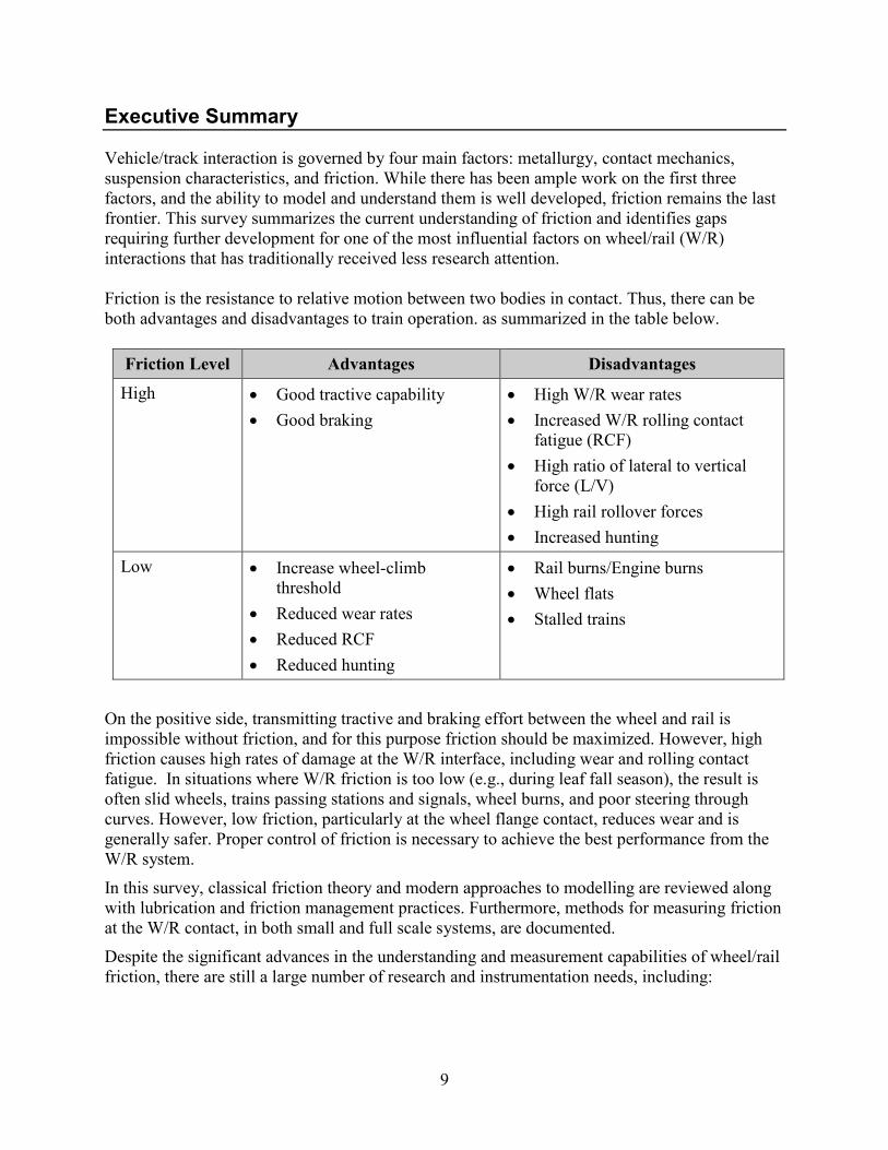
Vehicle/track interaction is governed by four main factors: metallurgy, contact mechanics, suspension characteristics, and friction. While there has been ample work on the first three factors, and the ability to model and understand them is well developed, friction remains the last frontier. This survey summarizes the current understanding of friction and identifies gaps requiring further development for one of the most influential factors on wheel/rail (W/R) interactions that has traditionally received less research attention. Friction is the resistance to relative motion between two bodies in contact. Thus, there can be both advantages and disadvantages to train operation. as summarized in the table below.
Friction Level Advantages Disadvantages
High • Good tractive capability • Good braking
• High W/R wear rates • Increased W/R rolling contact
fatigue (RCF) • High ratio of lateral to vertical
force (L/V) • High rail rollover forces • Increased hunting
Low • Increase wheel-climb threshold
• Reduced wear rates • Reduced RCF • Reduced hunting
• Rail burns/Engine burns • Wheel flats • Stalled trains
On the positive side, transmitting tractive and braking effort between the wheel and rail is impossible without friction, and for this purpose friction should be maximized. However, high friction causes high rates of damage at the W/R interface, including wear and rolling contact fatigue. In situations where W/R friction is too low (e.g., during leaf fall season), the result is often slid wheels, trains passing stations and signals, wheel burns, and poor steering through curves. However, low friction, particularly at the wheel flange contact, reduces wear and is generally safer. Proper control of friction is necessary to achieve the best performance from the W/R system.
In this survey, classical friction theory and modern approaches to modelling are reviewed along with lubrication and friction management practices. Furthermore, methods for measuring friction at the W/R contact, in both small and full scale systems, are documented.
Despite the significant advances in the understanding and measurement capabilities of wheel/rail friction, there are still a large number of research and instrumentation needs, including:
10
• Field measurement of the traction-creepage characteristic of real interfacial layers, and their collection into a “friction” library. This library would be used in dynamic simulation packages to model derailment, wear, RCF and vehicle stability.
• Even the collection of existing friction data would be of service to the rail community.
• A portable, self-contained and quick tool for characterizing the composition of interfacial layers in the field.
• Better increasing knowledge of the friction coefficient in the dry wheel flange contact.
• Improved rheological and lubricant consumption models to: o Understand how to most effectively achieve transfer of lubricants to the W/R
contact.
o Determine the “carry down” of lubricants along the track, especially when higher temperatures are involved.
• Establishing consensus on the number and identity of parameters required to adequately define the creepage-creep force relationship.
• Developing a method to logically and consistently apply the %KALKER approach to account for interfacial layers.
• Improving understanding of the friction characteristic at low temperatures.
• Improved adhesion enhancement agents that can show a value proposition compared with sand.
11
1. Introduction
Friction is the resistance to relative motion between two bodies in contact. It is a necessary feature of the human environment, where friction enables rubber tires to grab pavement and the human hand to grasp a basketball. However, there are many circumstances where friction is an unwanted feature, such as squeaking hinges, wear in car engines, and problems that develop in aging human hip joints.
The steel-wheel on steel-rail contact involves relatively smooth surfaces that are (generally) loaded with very high forces and often result in extremely high-contact pressures of 2000 MPa (290 ksi) or more. It is also an open system with a variety of contamination conditions that have dramatic effects on friction levels. As illustrated in Figure 1, the uncontrolled friction environment can experience friction coefficients that range from very low levels of about 0.05 to very high levels of about 0.7.
Figure 1: The uncontrolled wheel/rail interface has highly variable friction
1.1 Traction and Braking
Besides bearing the weight of the loaded axle, the W/R contact patch also transmits traction forces that are limited by the available friction. At the top of rail (TOR), the driving axles of the locomotives or power cars should operate with higher coefficients of friction to move the train forward and up hills, and to transmit braking effort to slow and halt the train. At the same time, the trailing cars should see lower friction so that rolling resistance and fuel consumption are minimized. The friction on the trailing axles should not be so low as to inhibit the contribution of
RAIN
no layerµ = 0.2 - 0.3
HUMID WEATHER SUNSHINE(no contaminants)
Fe203 and H20µ < 0.2
thick layer of Fe203µ = 0.6 - 0.7
COEFFICIENT OF FRICTION
0.05 TO 0.7rate of removal(chemical or mechanical)
film (no layer)µ = 0.05 - 0.2
weaken or strengthenthe layer
weakenthe layer
oil or grease inorganic contaminants(sand, clay, rust, etc.)
organic contaminants(leaves, hydrocarbons, etc.)
12
those trailing cars to the braking of the train. A train borne system for meeting this need is discussed in Section 4.2.1.
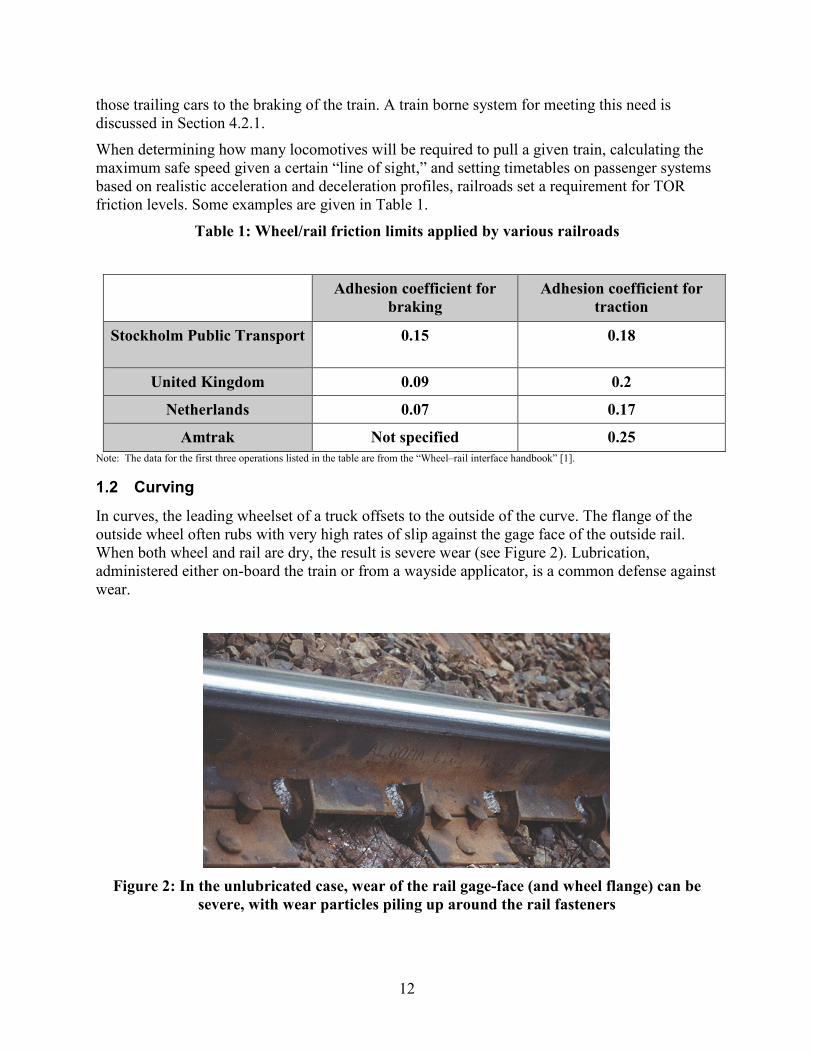
When determining how many locomotives will be required to pull a given train, calculating the maximum safe speed given a certain “line of sight,” and setting timetables on passenger systems based on realistic acceleration and deceleration profiles, railroads set a requirement for TOR friction levels. Some examples are given in Table 1.
Table 1: Wheel/rail friction limits applied by various railroads
Adhesion coefficient for braking
Adhesion coefficient for traction
Stockholm Public Transport 0.15 0.18
United Kingdom 0.09 0.2
Netherlands 0.07 0.17
Amtrak Not specified 0.25 Note: The data for the first three operations listed in the table are from the “Wheel–rail interface handbook” [1].
1.2 Curving
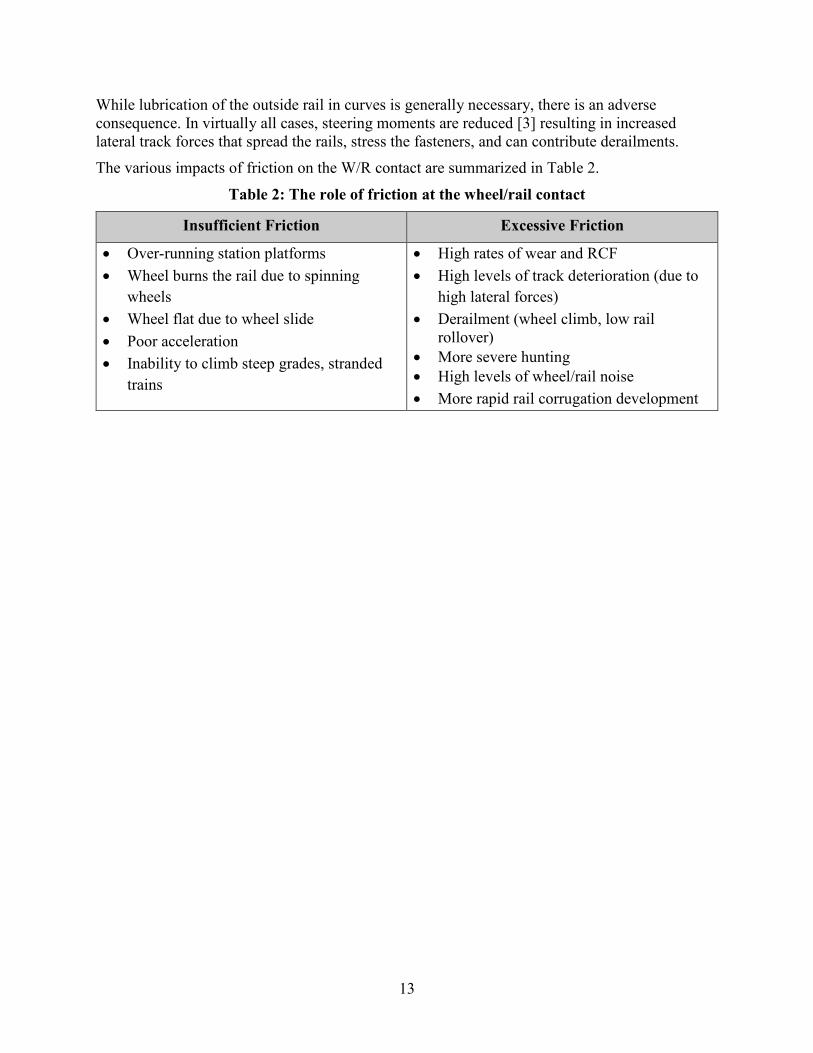
In curves, the leading wheelset of a truck offsets to the outside of the curve. The flange of the outside wheel often rubs with very high rates of slip against the gage face of the outside rail. When both wheel and rail are dry, the result is severe wear (see Figure 2). Lubrication, administered either on-board the train or from a wayside applicator, is a common defense against wear.
Figure 2: In the unlubricated case, wear of the rail gage-face (and wheel flange) can be
severe, with wear particles piling up around the rail fasteners
13
While lubrication of the outside rail in curves is generally necessary, there is an adverse consequence. In virtually all cases, steering moments are reduced [3] resulting in increased lateral track forces that spread the rails, stress the fasteners, and can contribute derailments.
The various impacts of friction on the W/R contact are summarized in Table 2.
Table 2: The role of friction at the wheel/rail contact
Insufficient Friction Excessive Friction
• Over-running station platforms • Wheel burns the rail due to spinning
wheels • Wheel flat due to wheel slide • Poor acceleration • Inability to climb steep grades, stranded
trains
• High rates of wear and RCF • High levels of track deterioration (due to
high lateral forces) • Derailment (wheel climb, low rail
rollover) • More severe hunting • High levels of wheel/rail noise • More rapid rail corrugation development
14
2. What is Friction?
2.1 Classical Theory
Friction is the resistive force that arises between two bodies in relative motion. Research from DaVinci (1599), Amontons (1699), and Coulomb (1785) form the following three laws of friction:
1. Friction is proportional to the normal force between surfaces.
2. Friction is independent of the nominal area of contact.
3. The kinetic friction is nearly independent of speed. Furthermore, it was generally understood that “kinetic friction” is generally less than “static” friction.
In its simplest form, friction force is proportional to the normal load (F ∝W) or F=µW.Explorations of friction have covered a range of mechanical and chemical mechanisms. The earliest explanation acknowledged that the contacting surfaces are rough on a micro-scale and that both normal and shear load is being borne by those asperities.
The Inclined Plane Model: Imagine two asperities in contact, with the average slope of the asperity being Θ. Further, the force required to move a load W up an inclined plane at an angle of Θ is FS=WtanΘ. The friction coefficient can then be identified as µ=tanΘ. While this explanation satisfies the previously mentioned three laws of friction, it has two deficiencies:
1. In case of very smooth surfaces, there is very often a high friction coefficient. This suggests that there are also chemical or molecular attraction forces involved1.
2. Once in motion, the surface would have some asperities sliding up the incline and others down with no net energy loss. Therefore, the bodies should continue sliding perpetually, but since energy is required to keep the bodies moving, there must be a dissipative mechanism operating.
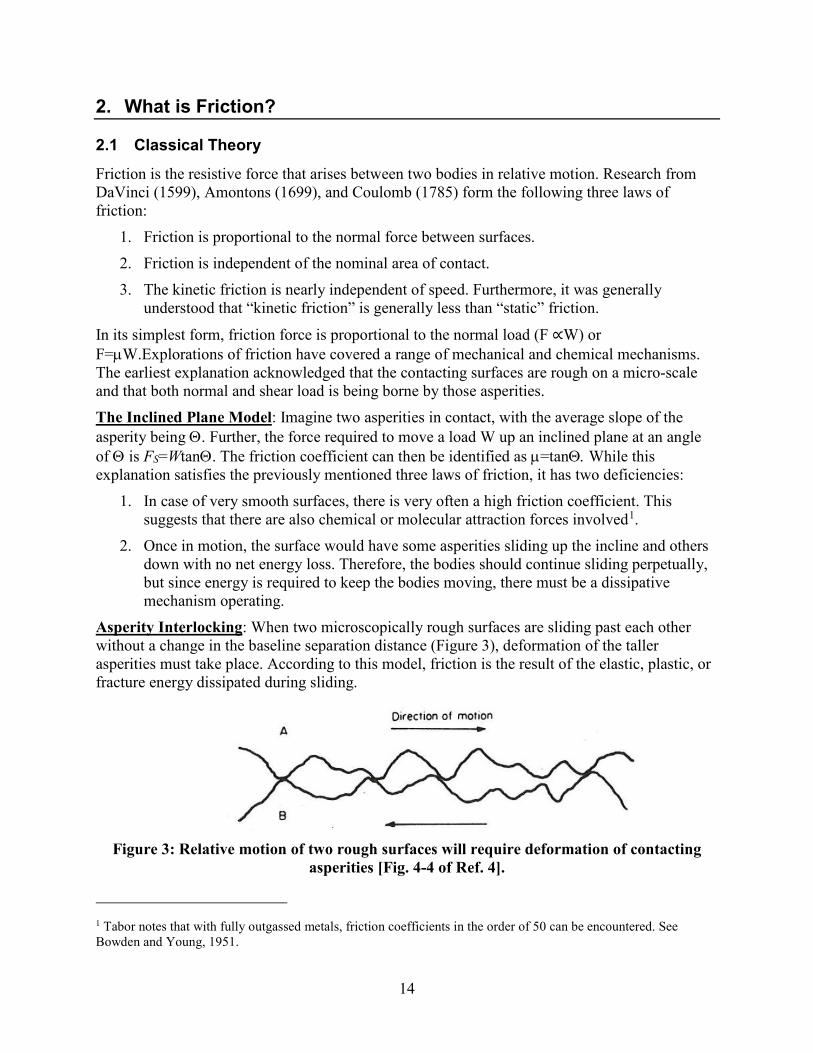
Asperity Interlocking: When two microscopically rough surfaces are sliding past each other without a change in the baseline separation distance (Figure 3), deformation of the taller asperities must take place. According to this model, friction is the result of the elastic, plastic, or fracture energy dissipated during sliding.
Figure 3: Relative motion of two rough surfaces will require deformation of contacting asperities [Fig. 4-4 of Ref. 4].
1 Tabor notes that with fully outgassed metals, friction coefficients in the order of 50 can be encountered. See Bowden and Young, 1951.
15
Cold Welding: The simple theory of Bowden and Tabor [5] presumes that pressures are very high at the asperity contacts (equivalent to the yield pressure of the material), and so the real area of contact AR = load /yield pressure = W/PY. At those locations of intimate metal-to-metal contact, the asperities effectively weld, and relative motion requires that those welded junctions break. The shearing stress S then must act along the real area of contact, such that the shear force FS = S×AR = S×W/PY and further that µ = FS/W = S/PY. This result says that friction is a function solely of the strength properties of the materials in contact. For an ideal plastic material, S is about 1/5th of PY [6], suggesting a rather invariant friction coefficient of about 0.2. However, since the measured friction coefficient varies significantly from 0.2, there are clearly additional factors at play in the general system.
Modified Adhesion Theory (Junction Growth): Tabor [7] understood the limits of their simplified approach and presented an improved model that recognized yield as resulting from combined normal and shear stresses. Yield of a two-dimensional asperity will be reached [8] when
P2+3S2=K2
When S=0, P=PY, so that K=PY and
P2+3S2 = PY2
If under normal loading the asperity has already yielded, then the increment of s can only be accompanied by a decrease in p (if we confine our discussion to the elastic-perfectly plastic case). Accordingly, the real area of contact AR must increase. In practice, this means that some of the individual asperity contact areas will increase in size while at the same time additional asperities may come into contact. In comparison with the Cold Welding Theory, the increase in AR with S allows for the larger coefficients of friction as measured in the practice.
For the generalized 3D asperity contact, it is presumed that a relationship of P2+αS2 = K2 holds. When S = 0, P = PY ⇒ P2+αS2 = PY
2. Based on empirical measurements it appears that α can vary between about 3 and 12 [7] with a value of 9 being most generally accepted.
At this point, there is no macroscopic sliding taking place. The surfaces are intimately connected at contacting asperities (junctions) whose individual areas and total number increase with normal and shear load. Under this model, the real area of contact continually increases with shear while the normal stress tends to zero. For perfectly clean surface this process could continue indefinitely with friction coefficients in the order of 10 being attained. The shear stress S is then approximately equal to the critical shear stress SY, W/AR is small compared with S/AR and αSY
2 ≃ PY
2. As noted from Tabor previously, PY≃5SY, which suggests that α=25. Experiments suggested lower values, hence the value of 9 used by Tabor subsequently.
To allow for sliding, it is necessary to introduce a contaminant film.
2.2 Influence of Contaminants
Assume that the two asperities in contact are separated by a film whose shear strength SF is some fraction of critical shear stress SY of the uncontaminated junction, i.e. SF = cSY. While the shear stress F/AR < SF, junction growth continues as discussed previously. However, when F/AR=SF, the film will shear, junction growth will cease, and local sliding will occur. Sliding will thus occur when
16
P2 + αSF2 = PY
2 [1]
But since PY2 = αSY
2 (shown previously), and SY = SF/c, we get P2 + αSF2 = α SF
2/c2
SF/P = µ = c / [α (1-c2)]1/2 [2]
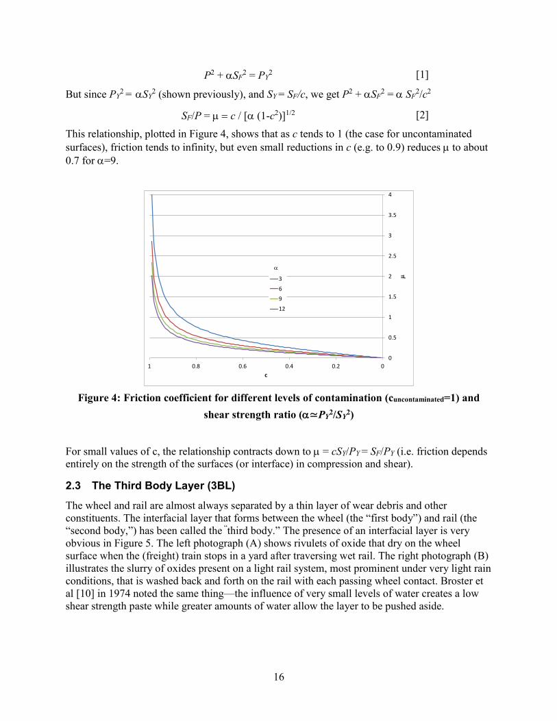
This relationship, plotted in Figure 4, shows that as c tends to 1 (the case for uncontaminated surfaces), friction tends to infinity, but even small reductions in c (e.g. to 0.9) reduces µ to about 0.7 for α=9.
Figure 4: Friction coefficient for different levels of contamination (cuncontaminated=1) and
shear strength ratio (α≃PY2/SY2)
For small values of c, the relationship contracts down to µ = cSY/PY = SF/PY (i.e. friction depends entirely on the strength of the surfaces (or interface) in compression and shear).
2.3 The Third Body Layer (3BL)
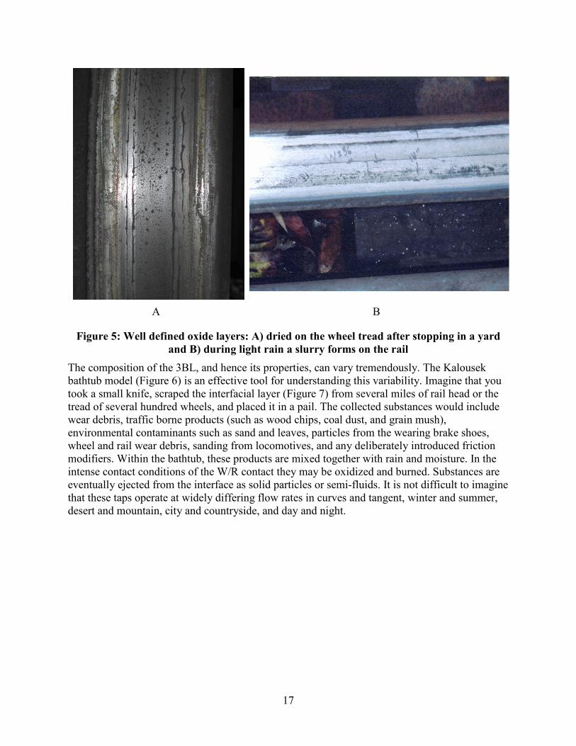
The wheel and rail are almost always separated by a thin layer of wear debris and other constituents. The interfacial layer that forms between the wheel (the “first body”) and rail (the “second body,”) has been called the “third body.” The presence of an interfacial layer is very obvious in Figure 5. The left photograph (A) shows rivulets of oxide that dry on the wheel surface when the (freight) train stops in a yard after traversing wet rail. The right photograph (B) illustrates the slurry of oxides present on a light rail system, most prominent under very light rain conditions, that is washed back and forth on the rail with each passing wheel contact. Broster et al [10] in 1974 noted the same thing—the influence of very small levels of water creates a low shear strength paste while greater amounts of water allow the layer to be pushed aside.
0
0.5
1
1.5
2
2.5
3
3.5
4
00.20.40.60.81
µ
c
3
6
9
12
α
17
A B
Figure 5: Well defined oxide layers: A) dried on the wheel tread after stopping in a yard and B) during light rain a slurry forms on the rail
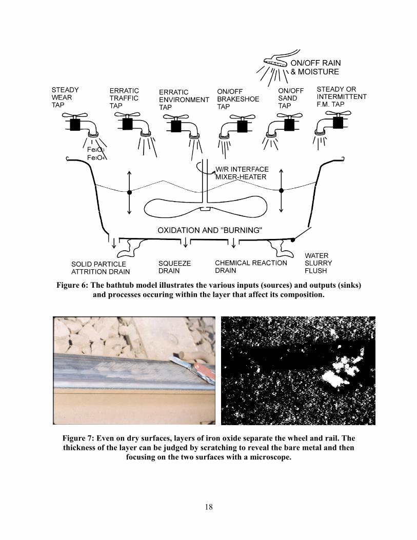
The composition of the 3BL, and hence its properties, can vary tremendously. The Kalousek bathtub model (Figure 6) is an effective tool for understanding this variability. Imagine that you took a small knife, scraped the interfacial layer (Figure 7) from several miles of rail head or the tread of several hundred wheels, and placed it in a pail. The collected substances would include wear debris, traffic borne products (such as wood chips, coal dust, and grain mush), environmental contaminants such as sand and leaves, particles from the wearing brake shoes, wheel and rail wear debris, sanding from locomotives, and any deliberately introduced friction modifiers. Within the bathtub, these products are mixed together with rain and moisture. In the intense contact conditions of the W/R contact they may be oxidized and burned. Substances are eventually ejected from the interface as solid particles or semi-fluids. It is not difficult to imagine that these taps operate at widely differing flow rates in curves and tangent, winter and summer, desert and mountain, city and countryside, and day and night.
18
Figure 6: The bathtub model illustrates the various inputs (sources) and outputs (sinks)
and processes occuring within the layer that affect its composition.
Figure 7: Even on dry surfaces, layers of iron oxide separate the wheel and rail. The thickness of the layer can be judged by scratching to reveal the bare metal and then
focusing on the two surfaces with a microscope.
19
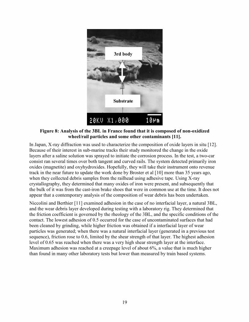
Figure 8: Analysis of the 3BL in France found that it is composed of non-oxidized
wheel/rail particles and some other contaminants [11]. In Japan, X-ray diffraction was used to characterize the composition of oxide layers in situ [12]. Because of their interest in sub-marine tracks their study monitored the change in the oxide layers after a saline solution was sprayed to initiate the corrosion process. In the test, a two-car consist ran several times over both tangent and curved rails. The system detected primarily iron oxides (magnetite) and oxyhydroxides. Hopefully, they will take their instrument onto revenue track in the near future to update the work done by Broster et al [10] more than 35 years ago, when they collected debris samples from the railhead using adhesive tape. Using X-ray crystallography, they determined that many oxides of iron were present, and subsequently that the bulk of it was from the cast-iron brake shoes that were in common use at the time. It does not appear that a contemporary analysis of the composition of wear debris has been undertaken.
Niccolini and Berthier [11] examined adhesion in the case of no interfacial layer, a natural 3BL, and the wear debris layer developed during testing with a laboratory rig. They determined that the friction coefficient is governed by the rheology of the 3BL, and the specific conditions of the contact. The lowest adhesion of 0.5 occurred for the case of uncontaminated surfaces that had been cleaned by grinding, while higher friction was obtained if a interfacial layer of wear particles was generated; when there was a natural interfacial layer (generated in a previous test sequence), friction rose to 0.6, limited by the shear strength of that layer. The highest adhesion level of 0.65 was reached when there was a very high shear strength layer at the interface. Maximum adhesion was reached at a creepage level of about 6%, a value that is much higher than found in many other laboratory tests but lower than measured by train based systems.
20
Figure 9: Portable X-ray diffraction analyzer with X-ray florescence capability.
During this testing the authors also arrived at boundaries of creepage, velocity, and contact pressure that would give strong adhesion but avoid wear particle generation. Outside of these boundaries, the activation energy was sufficient to trigger wear particle formation.
The W/R interfacial layers disintegrate and true metal-to-metal contact arises only under intense shearing and deformation, which can occur at the dry centre-plate/centre-bowl, as wheels are press-fitted onto the axle hub, where the friction wedge rubs against the column face in a truck/bogie and several other occasions in the vehicle and track systems. In W/R contact it is limited to the wheel-flange/gage-face region.
2.3.1 Dry contact of the wheel-flange/rail gage-face
When the wheel flange contacts the gage-face of the rail, there is a very high rate of slip; lateral creepages on a 75-degree flange angled wheel being typically in the order of 2% but reaching beyond 25% for very high angles of attack and a skewed truck frame2. Since gravity assists in eliminating debris from the interface, the wheel-flange/rail gage-face contact gives rise to metal-to-metal contact unless it is deliberately and conscientiously lubricated. As a result, the dry friction coefficient falls more along the lines of classical theory, being mostly dependent upon the ratio of shear strength to compressive strength of the surface layer. As per Section 2.1, an experimental value of α=9 produced a friction coefficient of around 0.35. A review of the literature for measurements of friction between the wheel-flange/rail gage-face were surprisingly fruitless. One suggested that “the friction coefficient between the self-cleaned wearing surface of flange and rail may be as high as 0.6,” [13] but unfortunately offered no substantiation. A query
2 Email from Dr. Wei Huang, NRC Jan 2013
21
to a colleague3 earned a reply that with a Salient push tribometer, “Our field experience is that dry gage face measurements are about 0.3.”
Most testing at high creepages has been on disc-on-disc systems that enable a 3BL to develop, representing top-of-rail contact conditions better than the gage face ones. Unfortunately, most operate only with longitudinal creepage and so there is no lateral creepage present to continually remove the interfacial layer, leading to unrealistically thick layers developing.
Other dry friction measurements using disc-on-disc [14] and pin-on-disc test rig [15] gave values of 0.6 and 0.5-0.75, respectively.
2.3.2 Leaf fall contamination
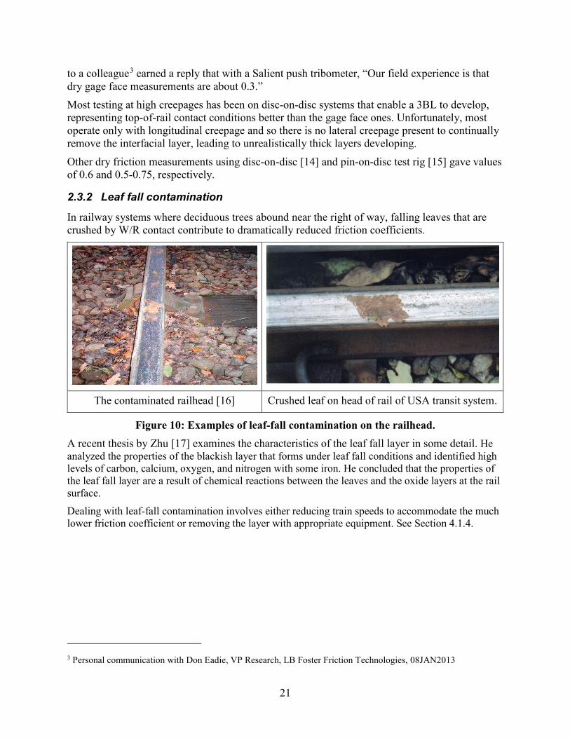
In railway systems where deciduous trees abound near the right of way, falling leaves that are crushed by W/R contact contribute to dramatically reduced friction coefficients.
The contaminated railhead [16] Crushed leaf on head of rail of USA transit system.
Figure 10: Examples of leaf-fall contamination on the railhead. A recent thesis by Zhu [17] examines the characteristics of the leaf fall layer in some detail. He analyzed the properties of the blackish layer that forms under leaf fall conditions and identified high levels of carbon, calcium, oxygen, and nitrogen with some iron. He concluded that the properties of the leaf fall layer are a result of chemical reactions between the leaves and the oxide layers at the rail surface.
Dealing with leaf-fall contamination involves either reducing train speeds to accommodate the much lower friction coefficient or removing the layer with appropriate equipment. See Section 4.1.4.
3 Personal communication with Don Eadie, VP Research, LB Foster Friction Technologies, 08JAN2013
22
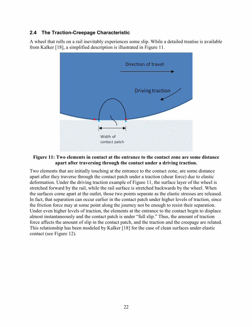
2.4 The Traction-Creepage Characteristic
A wheel that rolls on a rail inevitably experiences some slip. While a detailed treatise is available from Kalker [18], a simplified description is illustrated in Figure 11.
Figure 11: Two elements in contact at the entrance to the contact zone are some distance
apart after traversing through the contact under a driving traction. Two elements that are initially touching at the entrance to the contact zone, are some distance apart after they traverse through the contact patch under a traction (shear force) due to elastic deformation. Under the driving traction example of Figure 11, the surface layer of the wheel is stretched forward by the rail, while the rail surface is stretched backwards by the wheel. When the surfaces come apart at the outlet, those two points separate as the elastic stresses are released. In fact, that separation can occur earlier in the contact patch under higher levels of traction, since the friction force may at some point along the journey not be enough to resist their separation. Under even higher levels of traction, the elements at the entrance to the contact begin to displace almost instantaneously and the contact patch is under “full slip.” Thus, the amount of traction force affects the amount of slip in the contact patch, and the traction and the creepage are related. This relationship has been modeled by Kalker [18] for the case of clean surfaces under elastic contact (see Figure 12).
23
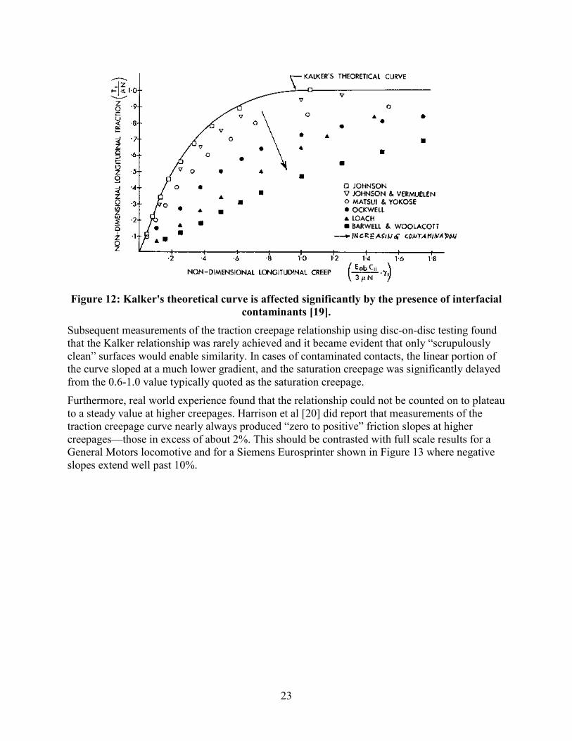
Figure 12: Kalker's theoretical curve is affected significantly by the presence of interfacial
contaminants [19]. Subsequent measurements of the traction creepage relationship using disc-on-disc testing found that the Kalker relationship was rarely achieved and it became evident that only “scrupulously clean” surfaces would enable similarity. In cases of contaminated contacts, the linear portion of the curve sloped at a much lower gradient, and the saturation creepage was significantly delayed from the 0.6-1.0 value typically quoted as the saturation creepage.
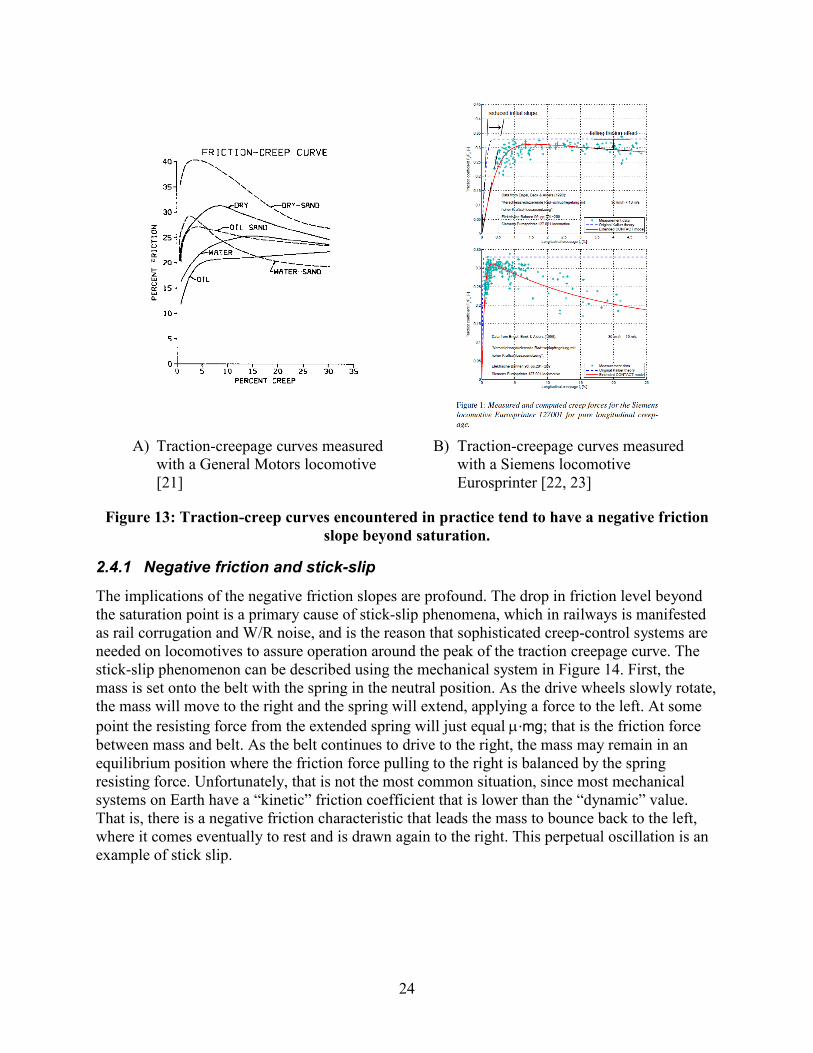
Furthermore, real world experience found that the relationship could not be counted on to plateau to a steady value at higher creepages. Harrison et al [20] did report that measurements of the traction creepage curve nearly always produced “zero to positive” friction slopes at higher creepages—those in excess of about 2%. This should be contrasted with full scale results for a General Motors locomotive and for a Siemens Eurosprinter shown in Figure 13 where negative slopes extend well past 10%.
24
A) Traction-creepage curves measured
with a General Motors locomotive [21]
B) Traction-creepage curves measured with a Siemens locomotive Eurosprinter [22, 23]
Figure 13: Traction-creep curves encountered in practice tend to have a negative friction slope beyond saturation.
2.4.1 Negative friction and stick-slip
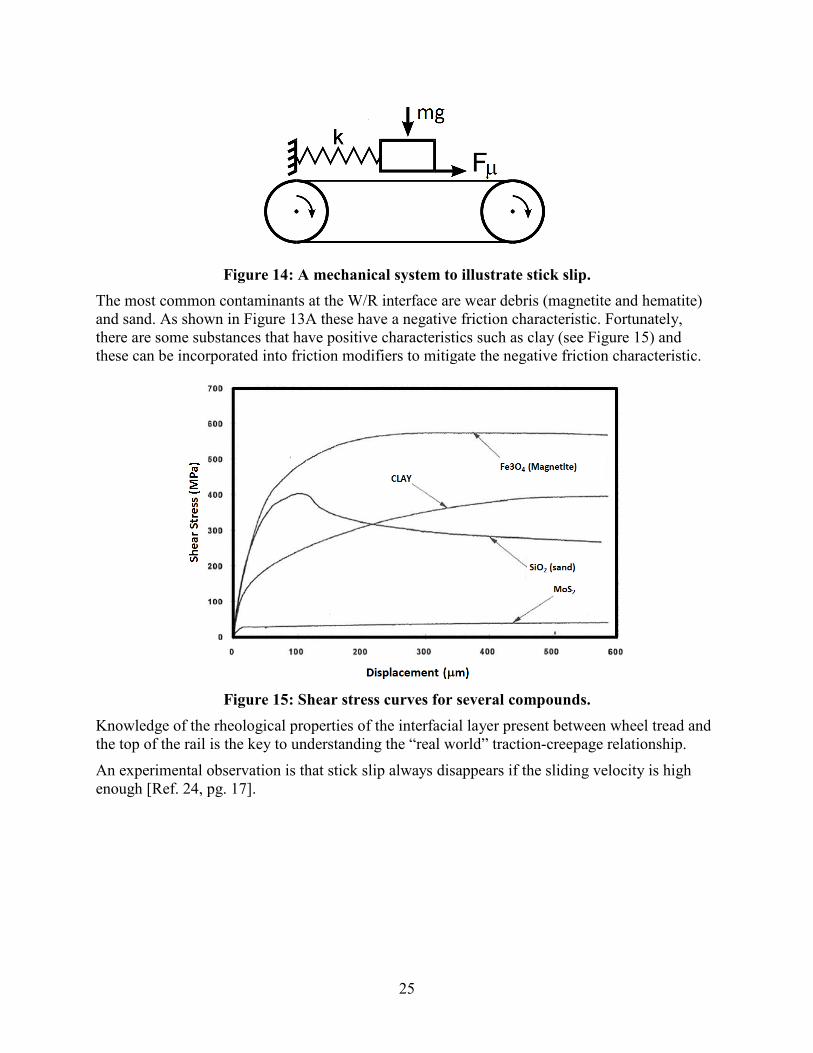
The implications of the negative friction slopes are profound. The drop in friction level beyond the saturation point is a primary cause of stick-slip phenomena, which in railways is manifested as rail corrugation and W/R noise, and is the reason that sophisticated creep-control systems are needed on locomotives to assure operation around the peak of the traction creepage curve. The stick-slip phenomenon can be described using the mechanical system in Figure 14. First, the mass is set onto the belt with the spring in the neutral position. As the drive wheels slowly rotate, the mass will move to the right and the spring will extend, applying a force to the left. At some point the resisting force from the extended spring will just equal µ∙mg; that is the friction force between mass and belt. As the belt continues to drive to the right, the mass may remain in an equilibrium position where the friction force pulling to the right is balanced by the spring resisting force. Unfortunately, that is not the most common situation, since most mechanical systems on Earth have a “kinetic” friction coefficient that is lower than the “dynamic” value. That is, there is a negative friction characteristic that leads the mass to bounce back to the left, where it comes eventually to rest and is drawn again to the right. This perpetual oscillation is an example of stick slip.
25
Figure 14: A mechanical system to illustrate stick slip.
The most common contaminants at the W/R interface are wear debris (magnetite and hematite) and sand. As shown in Figure 13A these have a negative friction characteristic. Fortunately, there are some substances that have positive characteristics such as clay (see Figure 15) and these can be incorporated into friction modifiers to mitigate the negative friction characteristic.
Figure 15: Shear stress curves for several compounds.
Knowledge of the rheological properties of the interfacial layer present between wheel tread and the top of the rail is the key to understanding the “real world” traction-creepage relationship.
An experimental observation is that stick slip always disappears if the sliding velocity is high enough [Ref. 24, pg. 17].
26
2.5 The Friction Circle
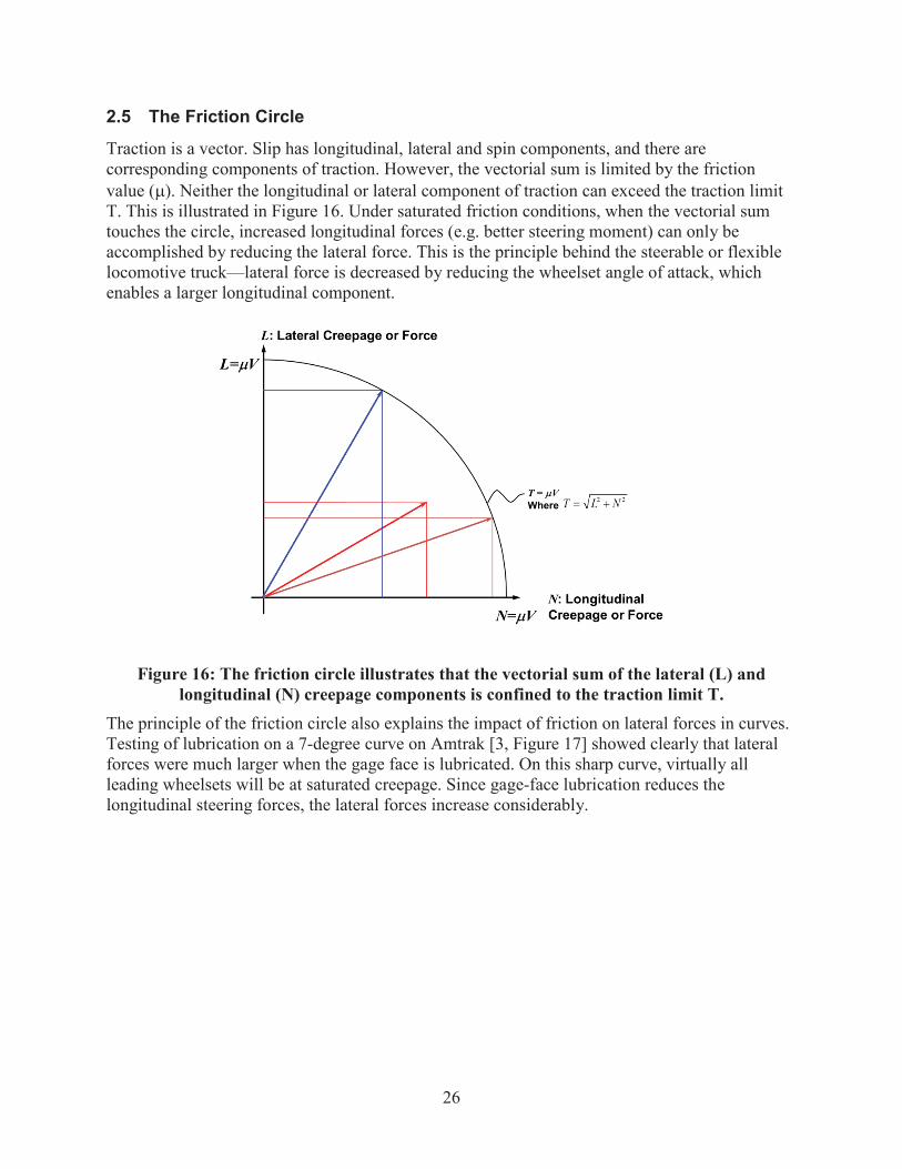
Traction is a vector. Slip has longitudinal, lateral and spin components, and there are corresponding components of traction. However, the vectorial sum is limited by the friction value ( ). Neither the longitudinal or lateral component of traction can exceed the traction limit T. This is illustrated in Figure 16. Under saturated friction conditions, when the vectorial sum touches the circle, increased longitudinal forces (e.g. better steering moment) can only be accomplished by reducing the lateral force. This is the principle behind the steerable or flexible locomotive truck—lateral force is decreased by reducing the wheelset angle of attack, which enables a larger longitudinal component.
Figure 16: The friction circle illustrates that the vectorial sum of the lateral (L) and longitudinal (N) creepage components is confined to the traction limit T.
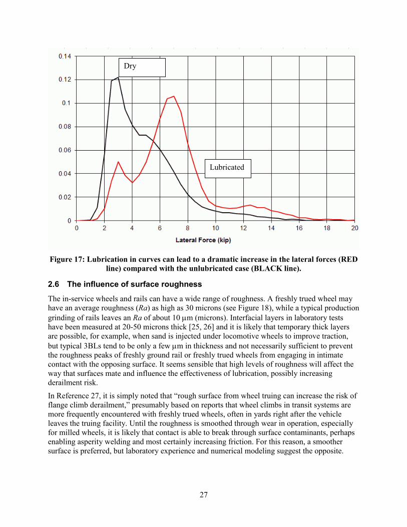
The principle of the friction circle also explains the impact of friction on lateral forces in curves. Testing of lubrication on a 7-degree curve on Amtrak [3, Figure 17] showed clearly that lateral forces were much larger when the gage face is lubricated. On this sharp curve, virtually all leading wheelsets will be at saturated creepage. Since gage-face lubrication reduces the longitudinal steering forces, the lateral forces increase considerably.
27
Figure 17: Lubrication in curves can lead to a dramatic increase in the lateral forces (RED
line) compared with the unlubricated case (BLACK line).
2.6 The influence of surface roughness
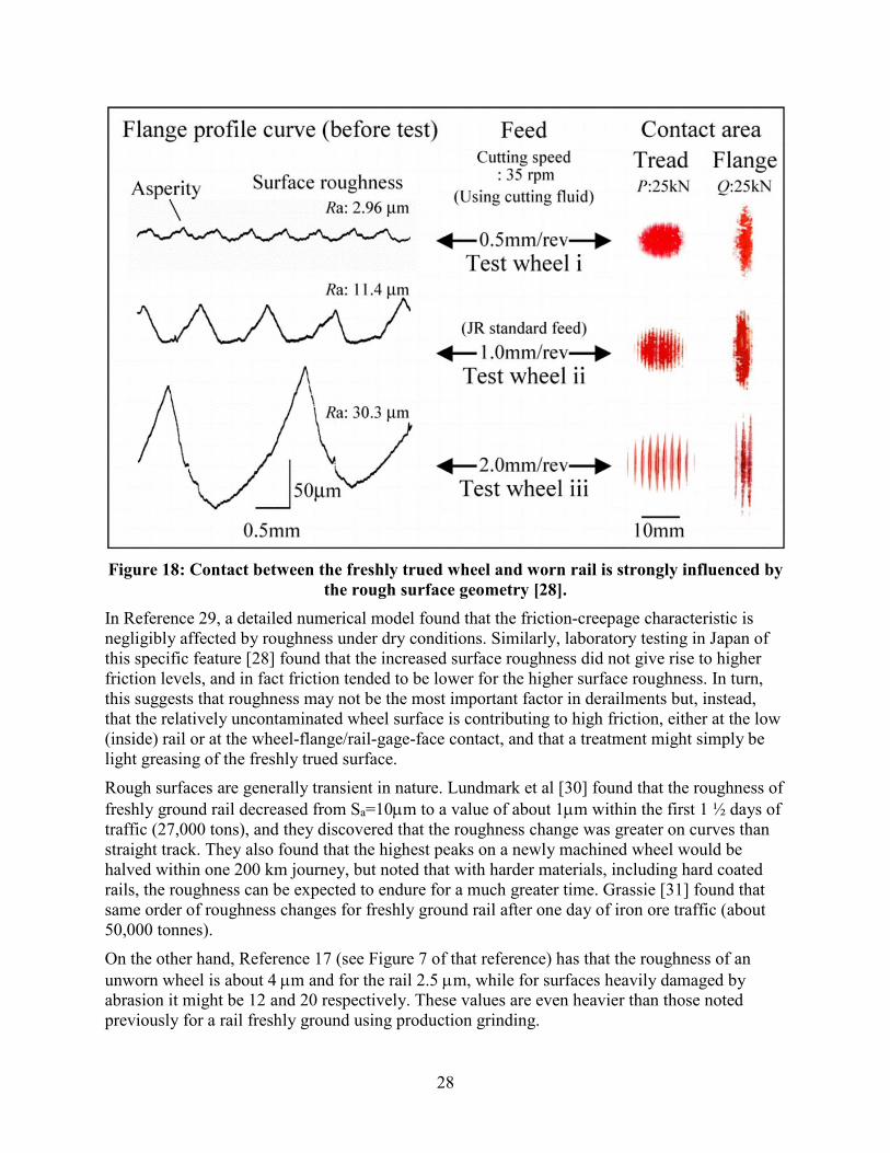
The in-service wheels and rails can have a wide range of roughness. A freshly trued wheel may have an average roughness (Ra) as high as 30 microns (see Figure 18), while a typical production grinding of rails leaves an Ra of about 10 µm (microns). Interfacial layers in laboratory tests have been measured at 20-50 microns thick [25, 26] and it is likely that temporary thick layers are possible, for example, when sand is injected under locomotive wheels to improve traction, but typical 3BLs tend to be only a few µm in thickness and not necessarily sufficient to prevent the roughness peaks of freshly ground rail or freshly trued wheels from engaging in intimate contact with the opposing surface. It seems sensible that high levels of roughness will affect the way that surfaces mate and influence the effectiveness of lubrication, possibly increasing derailment risk.
In Reference 27, it is simply noted that “rough surface from wheel truing can increase the risk of flange climb derailment,” presumably based on reports that wheel climbs in transit systems are more frequently encountered with freshly trued wheels, often in yards right after the vehicle leaves the truing facility. Until the roughness is smoothed through wear in operation, especially for milled wheels, it is likely that contact is able to break through surface contaminants, perhaps enabling asperity welding and most certainly increasing friction. For this reason, a smoother surface is preferred, but laboratory experience and numerical modeling suggest the opposite.
Lubricated
Dry
28
Figure 18: Contact between the freshly trued wheel and worn rail is strongly influenced by
the rough surface geometry [28]. In Reference 29, a detailed numerical model found that the friction-creepage characteristic is negligibly affected by roughness under dry conditions. Similarly, laboratory testing in Japan of this specific feature [28] found that the increased surface roughness did not give rise to higher friction levels, and in fact friction tended to be lower for the higher surface roughness. In turn, this suggests that roughness may not be the most important factor in derailments but, instead, that the relatively uncontaminated wheel surface is contributing to high friction, either at the low (inside) rail or at the wheel-flange/rail-gage-face contact, and that a treatment might simply be light greasing of the freshly trued surface.
Rough surfaces are generally transient in nature. Lundmark et al [30] found that the roughness of freshly ground rail decreased from Sa=10µm to a value of about 1µm within the first 1 ½ days of traffic (27,000 tons), and they discovered that the roughness change was greater on curves than straight track. They also found that the highest peaks on a newly machined wheel would be halved within one 200 km journey, but noted that with harder materials, including hard coated rails, the roughness can be expected to endure for a much greater time. Grassie [31] found that same order of roughness changes for freshly ground rail after one day of iron ore traffic (about 50,000 tonnes).
On the other hand, Reference 17 (see Figure 7 of that reference) has that the roughness of an unworn wheel is about 4 µm and for the rail 2.5 µm, while for surfaces heavily damaged by abrasion it might be 12 and 20 respectively. These values are even heavier than those noted previously for a rail freshly ground using production grinding.
29
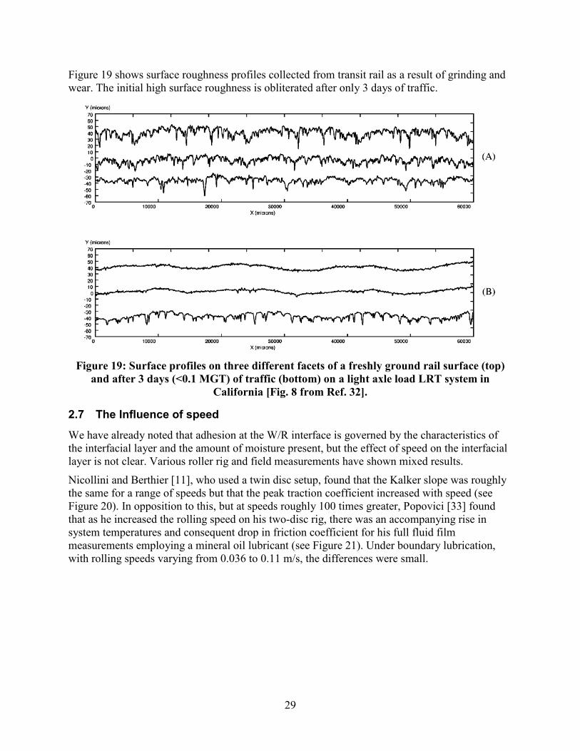
Figure 19 shows surface roughness profiles collected from transit rail as a result of grinding and wear. The initial high surface roughness is obliterated after only 3 days of traffic.
Figure 19: Surface profiles on three different facets of a freshly ground rail surface (top)
and after 3 days (<0.1 MGT) of traffic (bottom) on a light axle load LRT system in California [Fig. 8 from Ref. 32].
2.7 The Influence of speed
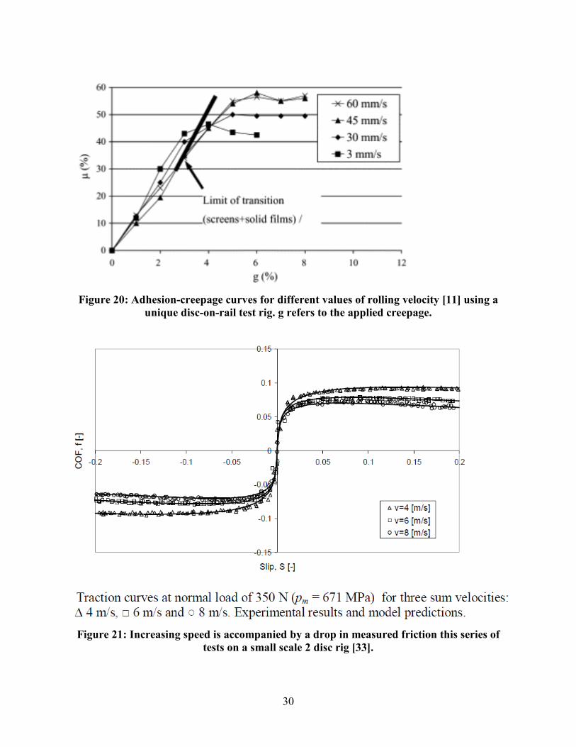
We have already noted that adhesion at the W/R interface is governed by the characteristics of the interfacial layer and the amount of moisture present, but the effect of speed on the interfacial layer is not clear. Various roller rig and field measurements have shown mixed results. Nicollini and Berthier [11], who used a twin disc setup, found that the Kalker slope was roughly the same for a range of speeds but that the peak traction coefficient increased with speed (see Figure 20). In opposition to this, but at speeds roughly 100 times greater, Popovici [33] found that as he increased the rolling speed on his two-disc rig, there was an accompanying rise in system temperatures and consequent drop in friction coefficient for his full fluid film measurements employing a mineral oil lubricant (see Figure 21). Under boundary lubrication, with rolling speeds varying from 0.036 to 0.11 m/s, the differences were small.
30
Figure 20: Adhesion-creepage curves for different values of rolling velocity [11] using a
unique disc-on-rail test rig. g refers to the applied creepage.
Figure 21: Increasing speed is accompanied by a drop in measured friction this series of
tests on a small scale 2 disc rig [33].
31
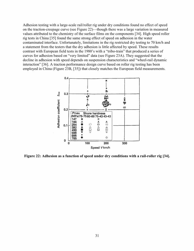
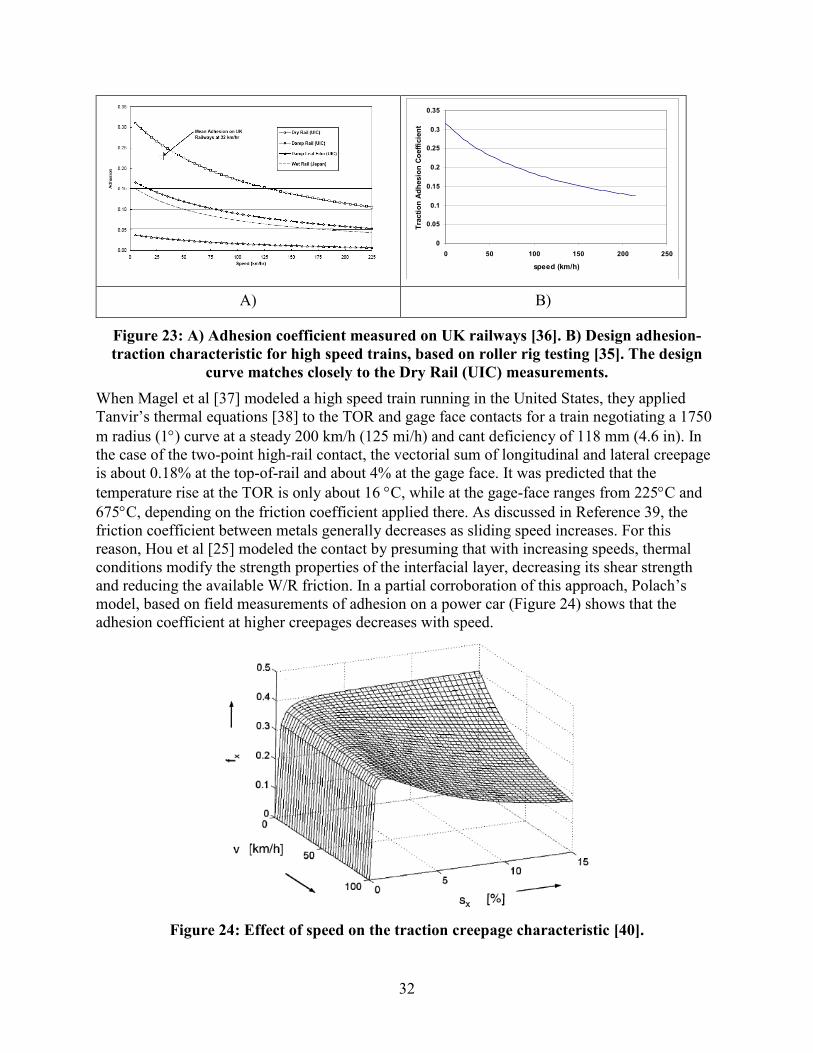
Adhesion testing with a large-scale rail/roller rig under dry conditions found no effect of speed on the traction-creepage curve (see Figure 22)—though there was a large variation in measured values attributed to the chemistry of the surface films on the components [34]. High speed roller rig tests in China [35] found the same strong effect of speed on adhesion in the water contaminated interface. Unfortunately, limitations in the rig restricted dry testing to 70 km/h and a statement from the testers that the dry adhesion is little affected by speed. These results contrast with European field tests in the 1980’s with a “tribo-train” that produced a series of curves for adhesion based on “very limited” data (see Figure 23A). They suggested that the decline in adhesion with speed depends on suspension characteristics and “wheel-rail dynamic interaction” [36]. A traction performance design curve based on roller rig testing has been employed in China (Figure 23B, [35]) that closely matches the European field measurements.
Figure 22: Adhesion as a function of speed under dry conditions with a rail-roller rig [34].
32
A) B)
Figure 23: A) Adhesion coefficient measured on UK railways [36]. B) Design adhesion-traction characteristic for high speed trains, based on roller rig testing [35]. The design
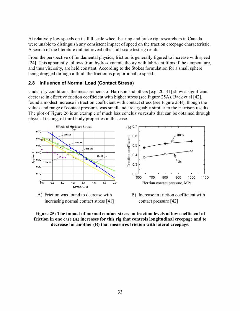
curve matches closely to the Dry Rail (UIC) measurements. When Magel et al [37] modeled a high speed train running in the United States, they applied Tanvir’s thermal equations [38] to the TOR and gage face contacts for a train negotiating a 1750 m radius (1°) curve at a steady 200 km/h (125 mi/h) and cant deficiency of 118 mm (4.6 in). In the case of the two-point high-rail contact, the vectorial sum of longitudinal and lateral creepage is about 0.18% at the top-of-rail and about 4% at the gage face. It was predicted that the temperature rise at the TOR is only about 16 °C, while at the gage-face ranges from 225°C and 675°C, depending on the friction coefficient applied there. As discussed in Reference 39, the friction coefficient between metals generally decreases as sliding speed increases. For this reason, Hou et al [25] modeled the contact by presuming that with increasing speeds, thermal conditions modify the strength properties of the interfacial layer, decreasing its shear strength and reducing the available W/R friction. In a partial corroboration of this approach, Polach’s model, based on field measurements of adhesion on a power car (Figure 24) shows that the adhesion coefficient at higher creepages decreases with speed.
Figure 24: Effect of speed on the traction creepage characteristic [40].
0
0.05
0.1
0.15
0.2
0.25
0.3
0.35
0 50 100 150 200 250
speed (km/h)
Trac
tion
Adhe
sion
Coe
ffici
ent
33
At relatively low speeds on its full-scale wheel-bearing and brake rig, researchers in Canada were unable to distinguish any consistent impact of speed on the traction creepage characteristic. A search of the literature did not reveal other full-scale test rig results.
From the perspective of fundamental physics, friction is generally figured to increase with speed [24]. This apparently follows from hydro-dynamic theory with lubricant films if the temperature, and thus viscosity, are held constant. According to the Stokes formulation for a small sphere being dragged through a fluid, the friction is proportional to speed.
2.8 Influence of Normal Load (Contact Stress)
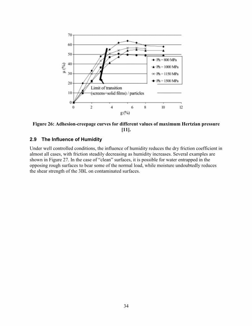
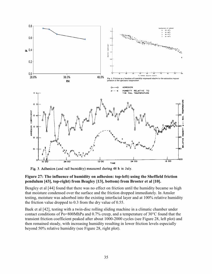
Under dry conditions, the measurements of Harrison and others [e.g. 20, 41] show a significant decrease in effective friction coefficient with higher stress (see Figure 25A). Baek et al [42], found a modest increase in traction coefficient with contact stress (see Figure 25B), though the values and range of contact pressures was small and are arguably similar to the Harrison results. The plot of Figure 26 is an example of much less conclusive results that can be obtained through physical testing, of third body properties in this case.
A) Friction was found to decrease with increasing normal contact stress [41]
B) Increase in friction coefficient with contact pressure [42]
Figure 25: The impact of normal contact stress on traction levels at low coefficient of friction in one case (A) increases for this rig that controls longitudinal creepage and to
decrease for another (B) that measures friction with lateral creepage.
34
Figure 26: Adhesion-creepage curves for different values of maximum Hertzian pressure
[11].
2.9 The Influence of Humidity
Under well controlled conditions, the influence of humidity reduces the dry friction coefficient in almost all cases, with friction steadily decreasing as humidity increases. Several examples are shown in Figure 27. In the case of “clean” surfaces, it is possible for water entrapped in the opposing rough surfaces to bear some of the normal load, while moisture undoubtedly reduces the shear strength of the 3BL on contaminated surfaces.
35
Figure 27: The influence of humidity on adhesion: top-left) using the Sheffield friction pendulum [43], top-right) from Beagley [13], bottom) from Broster et al [10]. Beagley et al [44] found that there was no effect on friction until the humidity became so high that moisture condensed over the surface and the friction dropped immediately. In Amsler testing, moisture was adsorbed into the existing interfacial layer and at 100% relative humidity the friction value dropped to 0.3 from the dry value of 0.55.
Baek et al [42], testing with a twin-disc rolling sliding machine in a climatic chamber under contact conditions of Po=800MhPa and 0.7% creep, and a temperature of 30°C found that the transient friction coefficient peaked after about 1000-2000 cycles (see Figure 28, left plot) and then remained steady, with increasing humidity resulting in lower friction levels especially beyond 50% relative humidity (see Figure 28, right plot).
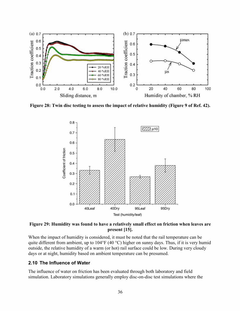
36
Figure 28: Twin disc testing to assess the impact of relative humidity (Figure 9 of Ref. 42).
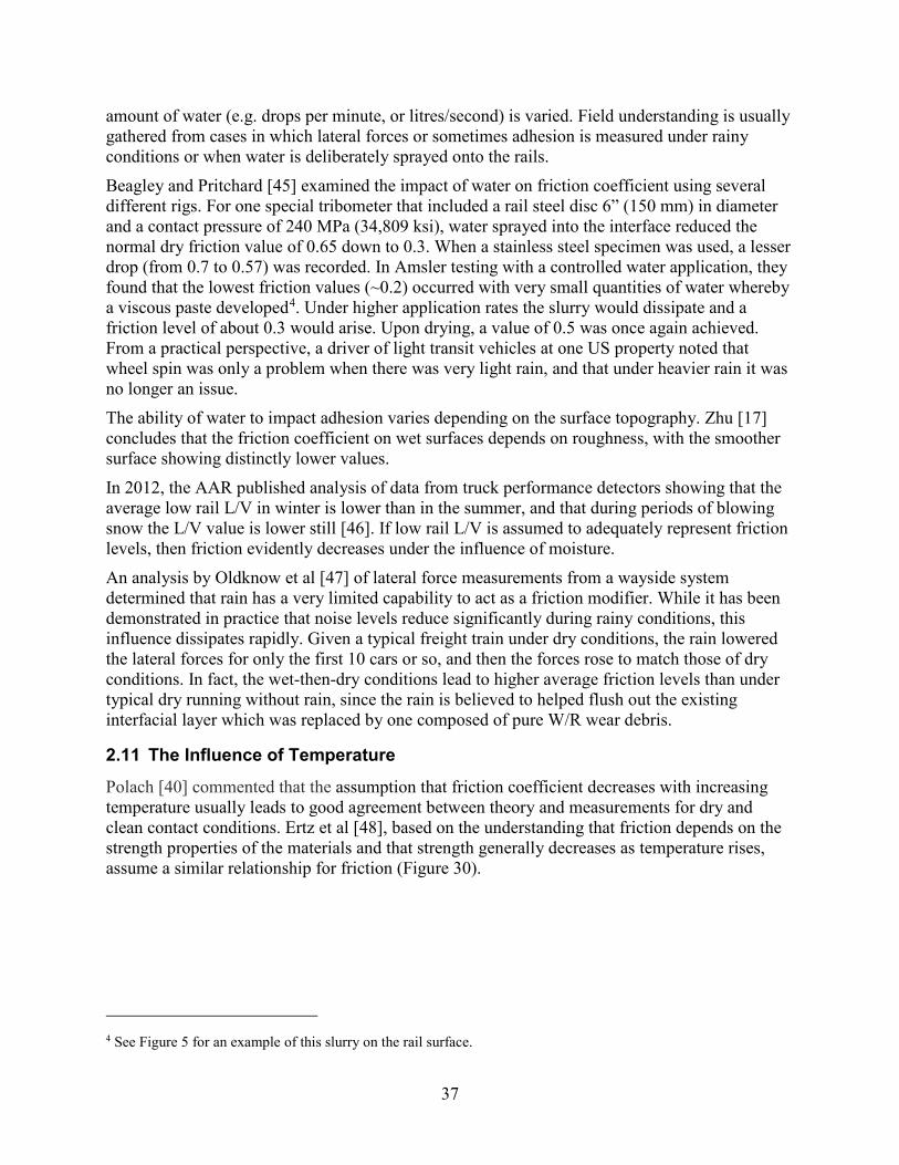
Figure 29: Humidity was found to have a relatively small effect on friction when leaves are
present [15]. When the impact of humidity is considered, it must be noted that the rail temperature can be quite different from ambient, up to 104°F (40 °C) higher on sunny days. Thus, if it is very humid outside, the relative humidity of a warm (or hot) rail surface could be low. During very cloudy days or at night, humidity based on ambient temperature can be presumed.
2.10 The Influence of Water
The influence of water on friction has been evaluated through both laboratory and field simulation. Laboratory simulations generally employ disc-on-disc test simulations where the
37
amount of water (e.g. drops per minute, or litres/second) is varied. Field understanding is usually gathered from cases in which lateral forces or sometimes adhesion is measured under rainy conditions or when water is deliberately sprayed onto the rails.
Beagley and Pritchard [45] examined the impact of water on friction coefficient using several different rigs. For one special tribometer that included a rail steel disc 6” (150 mm) in diameter and a contact pressure of 240 MPa (34,809 ksi), water sprayed into the interface reduced the normal dry friction value of 0.65 down to 0.3. When a stainless steel specimen was used, a lesser drop (from 0.7 to 0.57) was recorded. In Amsler testing with a controlled water application, they found that the lowest friction values (~0.2) occurred with very small quantities of water whereby a viscous paste developed4. Under higher application rates the slurry would dissipate and a friction level of about 0.3 would arise. Upon drying, a value of 0.5 was once again achieved. From a practical perspective, a driver of light transit vehicles at one US property noted that wheel spin was only a problem when there was very light rain, and that under heavier rain it was no longer an issue.
The ability of water to impact adhesion varies depending on the surface topography. Zhu [17] concludes that the friction coefficient on wet surfaces depends on roughness, with the smoother surface showing distinctly lower values.
In 2012, the AAR published analysis of data from truck performance detectors showing that the average low rail L/V in winter is lower than in the summer, and that during periods of blowing snow the L/V value is lower still [46]. If low rail L/V is assumed to adequately represent friction levels, then friction evidently decreases under the influence of moisture.
An analysis by Oldknow et al [47] of lateral force measurements from a wayside system determined that rain has a very limited capability to act as a friction modifier. While it has been demonstrated in practice that noise levels reduce significantly during rainy conditions, this influence dissipates rapidly. Given a typical freight train under dry conditions, the rain lowered the lateral forces for only the first 10 cars or so, and then the forces rose to match those of dry conditions. In fact, the wet-then-dry conditions lead to higher average friction levels than under typical dry running without rain, since the rain is believed to helped flush out the existing interfacial layer which was replaced by one composed of pure W/R wear debris.
2.11 The Influence of Temperature
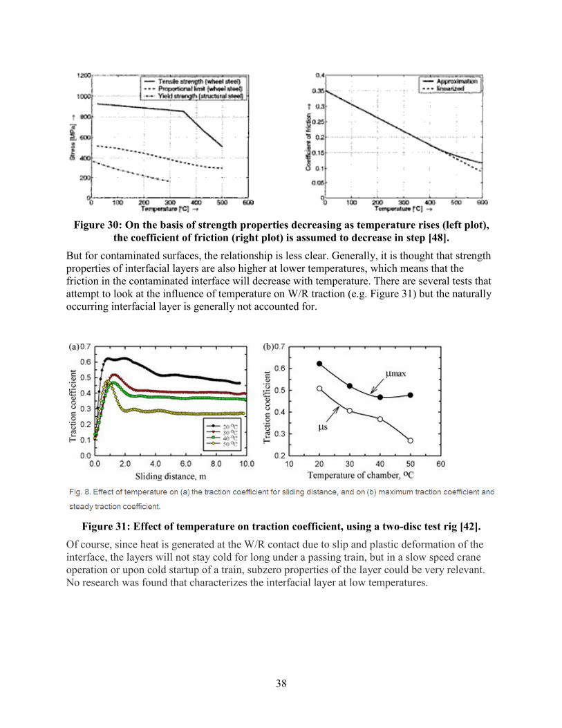
Polach [40] commented that the assumption that friction coefficient decreases with increasing temperature usually leads to good agreement between theory and measurements for dry and clean contact conditions. Ertz et al [48], based on the understanding that friction depends on the strength properties of the materials and that strength generally decreases as temperature rises, assume a similar relationship for friction (Figure 30).
4 See Figure 5 for an example of this slurry on the rail surface.
38
Figure 30: On the basis of strength properties decreasing as temperature rises (left plot),
the coefficient of friction (right plot) is assumed to decrease in step [48]. But for contaminated surfaces, the relationship is less clear. Generally, it is thought that strength properties of interfacial layers are also higher at lower temperatures, which means that the friction in the contaminated interface will decrease with temperature. There are several tests that attempt to look at the influence of temperature on W/R traction (e.g. Figure 31) but the naturally occurring interfacial layer is generally not accounted for.
Figure 31: Effect of temperature on traction coefficient, using a two-disc test rig [42].
Of course, since heat is generated at the W/R contact due to slip and plastic deformation of the interface, the layers will not stay cold for long under a passing train, but in a slow speed crane operation or upon cold startup of a train, subzero properties of the layer could be very relevant. No research was found that characterizes the interfacial layer at low temperatures.
39
3. Friction Modeling
Kalker’s theory for rolling contact is the most widely used model for W/R simulations. However, additional modifications were made to the theory to address several experimentally observed features, including the negative traction/creep characteristic beyond saturation and apparent dependencies of traction on speed and normal contact pressure.
3.1 Velocity Accommodation
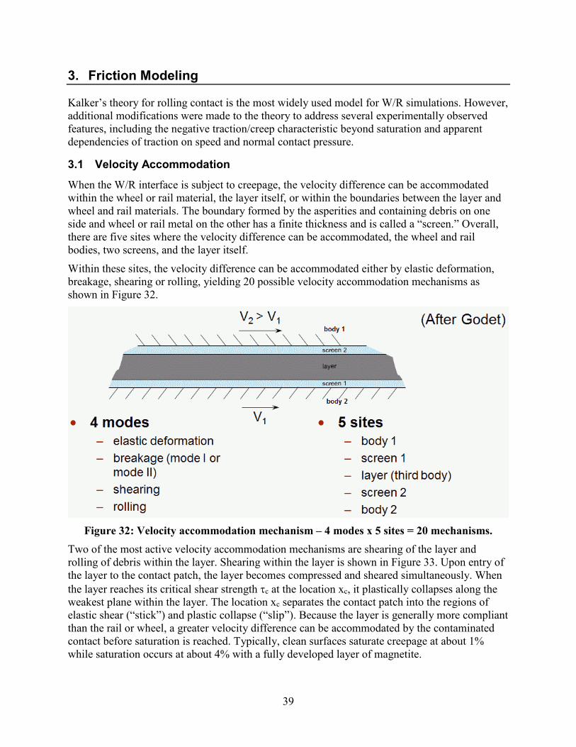
When the W/R interface is subject to creepage, the velocity difference can be accommodated within the wheel or rail material, the layer itself, or within the boundaries between the layer and wheel and rail materials. The boundary formed by the asperities and containing debris on one side and wheel or rail metal on the other has a finite thickness and is called a “screen.” Overall, there are five sites where the velocity difference can be accommodated, the wheel and rail bodies, two screens, and the layer itself.
Within these sites, the velocity difference can be accommodated either by elastic deformation, breakage, shearing or rolling, yielding 20 possible velocity accommodation mechanisms as shown in Figure 32.
Figure 32: Velocity accommodation mechanism – 4 modes x 5 sites = 20 mechanisms.
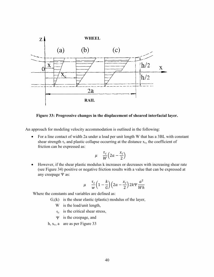
Two of the most active velocity accommodation mechanisms are shearing of the layer and rolling of debris within the layer. Shearing within the layer is shown in Figure 33. Upon entry of the layer to the contact patch, the layer becomes compressed and sheared simultaneously. When the layer reaches its critical shear strength τc at the location xc, it plastically collapses along the weakest plane within the layer. The location xc separates the contact patch into the regions of elastic shear (“stick”) and plastic collapse (“slip”). Because the layer is generally more compliant than the rail or wheel, a greater velocity difference can be accommodated by the contaminated contact before saturation is reached. Typically, clean surfaces saturate creepage at about 1% while saturation occurs at about 4% with a fully developed layer of magnetite.
40
Figure 33: Progressive changes in the displacement of sheared interfacial layer.
An approach for modeling velocity accommodation is outlined in the following:
• For a line contact of width 2a under a load per unit length W that has a 3BL with constant shear strength τc and plastic collapse occurring at the distance xc, the coefficient of friction can be expressed as:
𝜇𝜇 =𝜏𝜏𝑐𝑐𝑊𝑊�2𝑎𝑎 −
𝑥𝑥𝑐𝑐2�
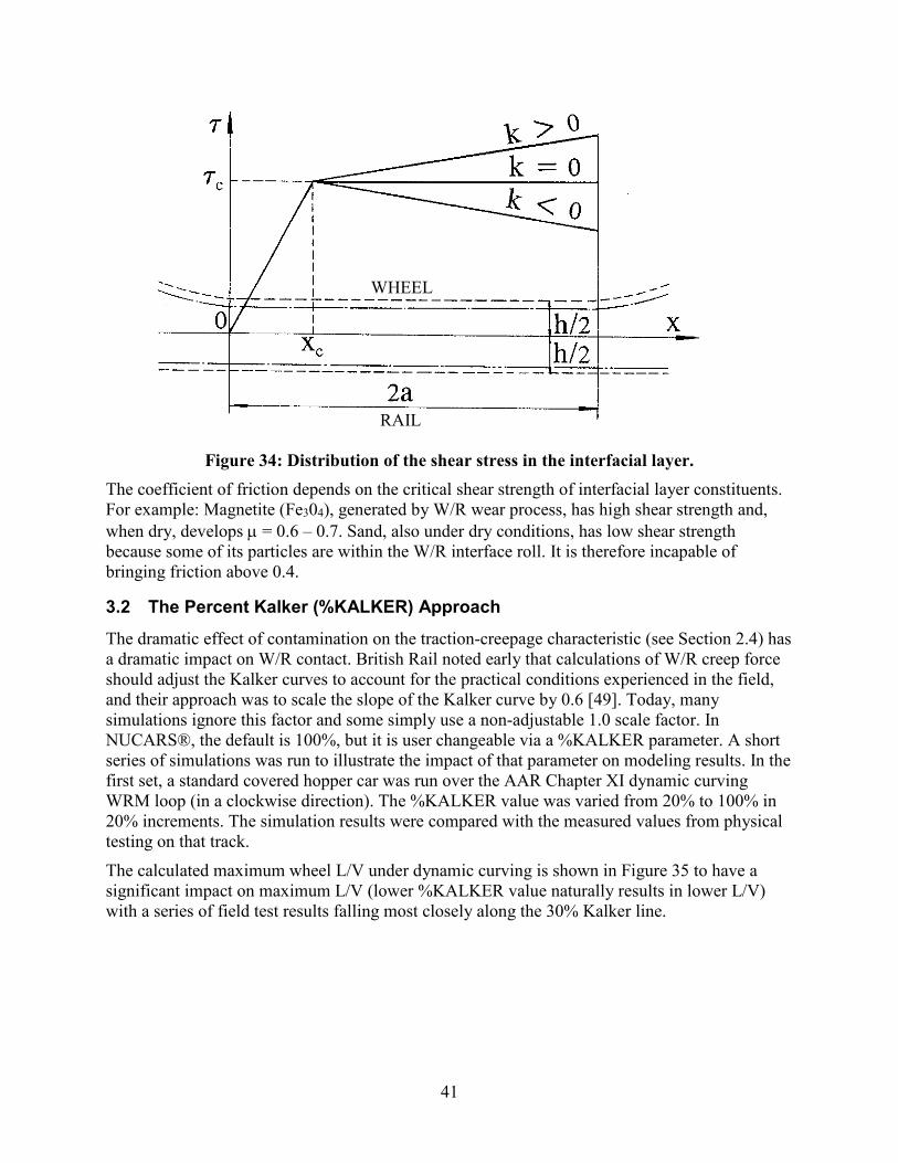
• However, if the shear plastic modulus k increases or decreases with increasing shear rate (see Figure 34) positive or negative friction results with a value that can be expressed at any creepage Ψ as:
𝜇𝜇 =𝜏𝜏𝑐𝑐𝑤𝑤�1 −
𝑘𝑘𝐺𝐺� �2𝑎𝑎 −
𝑥𝑥𝑐𝑐2�2𝑘𝑘Ψ
𝑎𝑎2
𝑊𝑊ℎ
Where the constants and variables are defined as: G,(k) is the shear elastic (plastic) modulus of the layer,
W is the load/unit length, τc is the critical shear stress, Ψ is the creepage, and
h, xc, a are as per Figure 33
WHEEL
RAIL
41
Figure 34: Distribution of the shear stress in the interfacial layer.
The coefficient of friction depends on the critical shear strength of interfacial layer constituents. For example: Magnetite (Fe304), generated by W/R wear process, has high shear strength and, when dry, develops µ = 0.6 – 0.7. Sand, also under dry conditions, has low shear strength because some of its particles are within the W/R interface roll. It is therefore incapable of bringing friction above 0.4.
3.2 The Percent Kalker (%KALKER) Approach
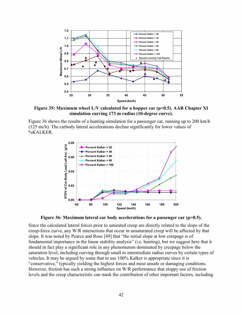
The dramatic effect of contamination on the traction-creepage characteristic (see Section 2.4) has a dramatic impact on W/R contact. British Rail noted early that calculations of W/R creep force should adjust the Kalker curves to account for the practical conditions experienced in the field, and their approach was to scale the slope of the Kalker curve by 0.6 [49]. Today, many simulations ignore this factor and some simply use a non-adjustable 1.0 scale factor. In NUCARS®, the default is 100%, but it is user changeable via a %KALKER parameter. A short series of simulations was run to illustrate the impact of that parameter on modeling results. In the first set, a standard covered hopper car was run over the AAR Chapter XI dynamic curving WRM loop (in a clockwise direction). The %KALKER value was varied from 20% to 100% in 20% increments. The simulation results were compared with the measured values from physical testing on that track.
The calculated maximum wheel L/V under dynamic curving is shown in Figure 35 to have a significant impact on maximum L/V (lower %KALKER value naturally results in lower L/V) with a series of field test results falling most closely along the 30% Kalker line.
WHEEL
RAIL
42
Figure 35: Maximum wheel L/V calculated for a hopper car (μ=0.5). AAR Chapter XI
simulation curving 173 m radius (10-degree curve). Figure 36 shows the results of a hunting simulation for a passenger car, running up to 200 km/h (125 mi/h). The carbody lateral accelerations decline significantly for lower values of %KALKER.
Figure 36: Maximum lateral car body accelerations for a passenger car (μ=0.5).
Since the calculated lateral forces prior to saturated creep are directly related to the slope of the creep-force curve, any W/R interactions that occur in unsaturated creep will be affected by that slope. It was noted by Pearce and Rose [49] that “the initial slope at low creepage is of fundamental importance in the linear stability analysis” (i.e. hunting), but we suggest here that it should in fact play a significant role in any phenomenon dominated by creepage below the saturation level, including curving through small to intermediate radius curves by certain types of vehicles. It may be argued by some that to use 100% Kalker is appropriate since it is “conservative,” typically yielding the highest forces and most unsafe or damaging conditions. However, friction has such a strong influence on W/R performance that sloppy use of friction levels and the creep characteristic can mask the contribution of other important factors, including
0.4
0.5
0.6
0.7
0.8
0.9
1.0
1.1
1.2
25 30 35 40 45 50 55
Max
imum
Whe
el L
/V
Speed (km/h)
Percent Kalker = 20
Percent Kalker = 30
Percent Kalker = 40
Percent Kalker = 60
Percent Kalker = 80
Percent Kalker = 100
Dynamic Curving Test Results
0.00
0.02
0.04
0.06
0.08
60 80 100 120 140 160 180 200Speed (km/h)
STD
V of
Car
Bod
y Le
ad L
atl A
cc. (
g's) Percent Kalker = 20
Percent Kalker = 40Percent Kalker = 60Percent Kalker = 80Percent Kalker = 100
43
the impact of vehicle characteristics (which are often the focus of many dynamic simulations in the first place).
Wheel climb and lateral force derailments, on the other hand, are governed by the absolute friction levels obtained in saturated creep and the simple friction limit should be sufficient.
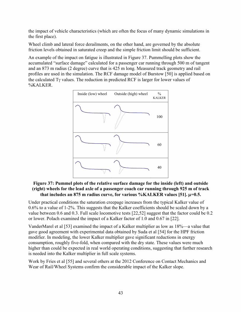
An example of the impact on fatigue is illustrated in Figure 37. Pummelling plots show the accumulated “surface damage” calculated for a passenger car running through 500 m of tangent and an 873 m radius (2 degree) curve that is 425 m long. Measured track geometry and rail profiles are used in the simulation. The RCF damage model of Burstow [50] is applied based on the calculated Tγ values. The reduction in predicted RCF is larger for lower values of %KALKER.
Inside (low) wheel Outside (high) wheel % KALKER
100
60
40
Figure 37: Pummel plots of the relative surface damage for the inside (left) and outside (right) wheels for the lead axle of a passenger coach car running through 925 m of track
that includes an 875 m radius curve, for various %KALKER values [51]. µ=0.5. Under practical conditions the saturation creepage increases from the typical Kalker value of 0.6% to a value of 1-2%. This suggests that the Kalker coefficients should be scaled down by a value between 0.6 and 0.3. Full scale locomotive tests [22,52] suggest that the factor could be 0.2 or lower. Polach examined the impact of a Kalker factor of 1.0 and 0.67 in [22].
VanderMarel et al [53] examined the impact of a Kalker multiplier as low as 18%—a value that gave good agreement with experimental data obtained by Suda et al [54] for the HPF friction modifier. In modeling, the lower Kalker multiplier gave significant reductions in energy consumption, roughly five-fold, when compared with the dry state. These values were much higher than could be expected in real world operating conditions, suggesting that further research is needed into the Kalker multiplier in full scale systems.
Work by Fries et al [55] and several others at the 2012 Conference on Contact Mechanics and Wear of Rail/Wheel Systems confirm the considerable impact of the Kalker slope.
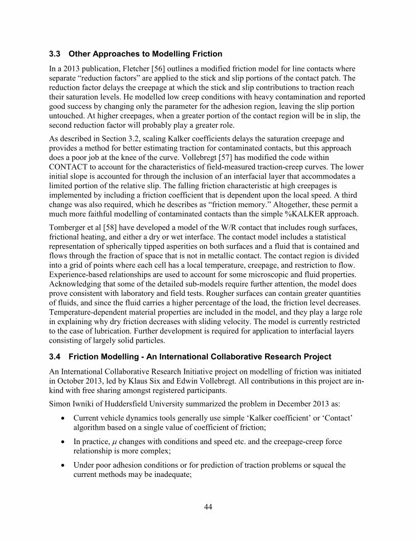
44
3.3 Other Approaches to Modelling Friction
In a 2013 publication, Fletcher [56] outlines a modified friction model for line contacts where separate “reduction factors” are applied to the stick and slip portions of the contact patch. The reduction factor delays the creepage at which the stick and slip contributions to traction reach their saturation levels. He modelled low creep conditions with heavy contamination and reported good success by changing only the parameter for the adhesion region, leaving the slip portion untouched. At higher creepages, when a greater portion of the contact region will be in slip, the second reduction factor will probably play a greater role.
As described in Section 3.2, scaling Kalker coefficients delays the saturation creepage and provides a method for better estimating traction for contaminated contacts, but this approach does a poor job at the knee of the curve. Vollebregt [57] has modified the code within CONTACT to account for the characteristics of field-measured traction-creep curves. The lower initial slope is accounted for through the inclusion of an interfacial layer that accommodates a limited portion of the relative slip. The falling friction characteristic at high creepages is implemented by including a friction coefficient that is dependent upon the local speed. A third change was also required, which he describes as “friction memory.” Altogether, these permit a much more faithful modelling of contaminated contacts than the simple %KALKER approach.
Tomberger et al [58] have developed a model of the W/R contact that includes rough surfaces, frictional heating, and either a dry or wet interface. The contact model includes a statistical representation of spherically tipped asperities on both surfaces and a fluid that is contained and flows through the fraction of space that is not in metallic contact. The contact region is divided into a grid of points where each cell has a local temperature, creepage, and restriction to flow. Experience-based relationships are used to account for some microscopic and fluid properties. Acknowledging that some of the detailed sub-models require further attention, the model does prove consistent with laboratory and field tests. Rougher surfaces can contain greater quantities of fluids, and since the fluid carries a higher percentage of the load, the friction level decreases. Temperature-dependent material properties are included in the model, and they play a large role in explaining why dry friction decreases with sliding velocity. The model is currently restricted to the case of lubrication. Further development is required for application to interfacial layers consisting of largely solid particles.
3.4 Friction Modelling - An International Collaborative Research Project
An International Collaborative Research Initiative project on modelling of friction was initiated in October 2013, led by Klaus Six and Edwin Vollebregt. All contributions in this project are in-kind with free sharing amongst registered participants. Simon Iwniki of Huddersfield University summarized the problem in December 2013 as:
• Current vehicle dynamics tools generally use simple ‘Kalker coefficient’ or ‘Contact’ algorithm based on a single value of coefficient of friction;
• In practice, µ changes with conditions and speed etc. and the creepage-creep force relationship is more complex;
• Under poor adhesion conditions or for prediction of traction problems or squeal the current methods may be inadequate;
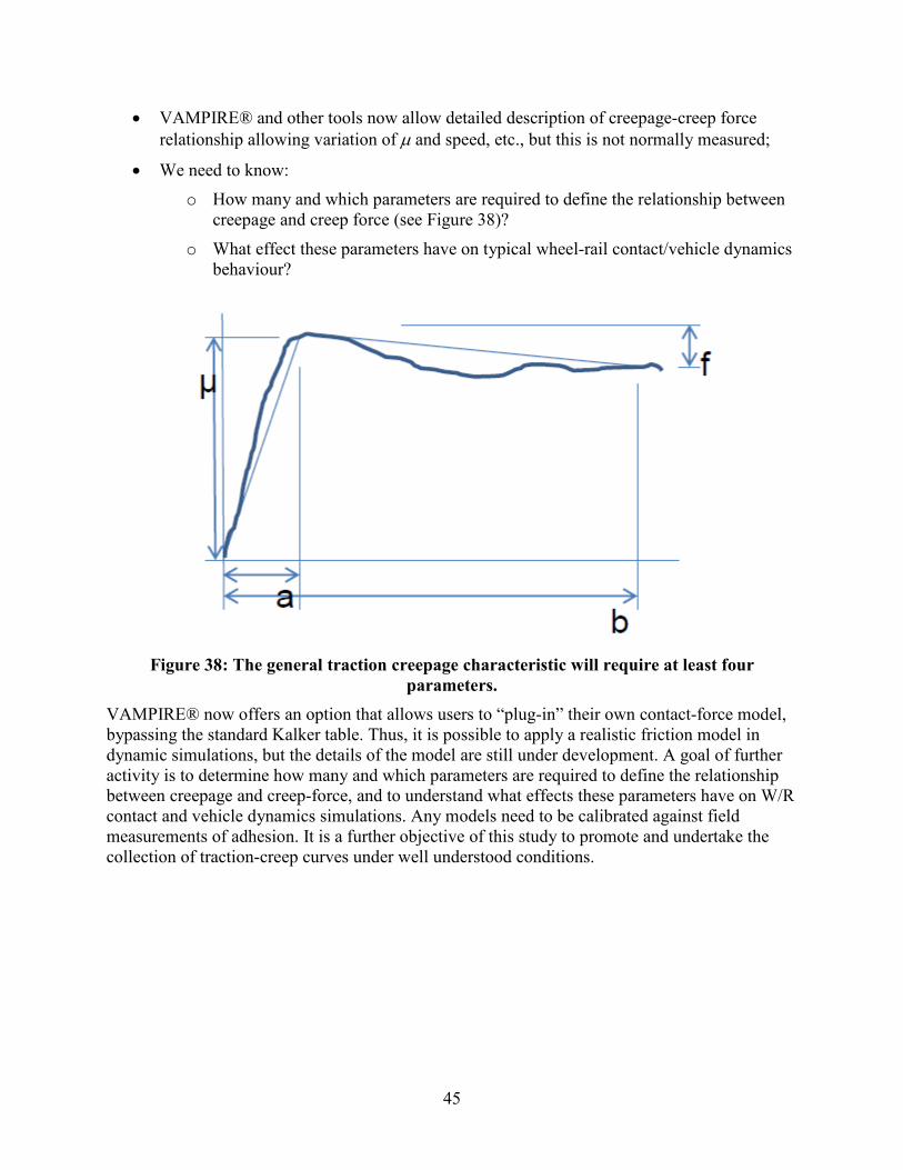
45
• VAMPIRE® and other tools now allow detailed description of creepage-creep force relationship allowing variation of µ and speed, etc., but this is not normally measured;
• We need to know: o How many and which parameters are required to define the relationship between
creepage and creep force (see Figure 38)?
o What effect these parameters have on typical wheel-rail contact/vehicle dynamics behaviour?
Figure 38: The general traction creepage characteristic will require at least four
parameters. VAMPIRE® now offers an option that allows users to “plug-in” their own contact-force model, bypassing the standard Kalker table. Thus, it is possible to apply a realistic friction model in dynamic simulations, but the details of the model are still under development. A goal of further activity is to determine how many and which parameters are required to define the relationship between creepage and creep-force, and to understand what effects these parameters have on W/R contact and vehicle dynamics simulations. Any models need to be calibrated against field measurements of adhesion. It is a further objective of this study to promote and undertake the collection of traction-creep curves under well understood conditions.
46
4. Friction Control
Friction control can assist in accomplishing many goals that locomotive, vehicle, operators, designers, as well as track maintenance managers, would like to attain:
• High dispatchable adhesion on locomotives. This is the minimum traction force that a locomotive can achieve under adverse conditions (such as contamination from oil or water). Sand is often used to improve adhesion between wheel and rail, and under dry conditions, it can develop a coefficient of friction about 0.4 (see Figure 13 A), but at the same time it abrades the locomotive wheels and fouls the ballast. Although railways would like to replace sanding, it is such a low-cost product that it is hard to imagine an affordable alternative.
• Low wear. This is achieved primarily through lubrication of the outer rail, but as noted in Reference 59, in the absence of top-of-rail contamination, the rates of lateral wear can be very high in curves.
• Alleviation of contact fatigue defects. By moderating high friction conditions at the W/R running band, a friction modifier reduces the traction forces that are a major contributor to rolling contact fatigue [see Figure 39, Ref. 60].
Figure 39: The effect of friction management of wear and RCF – full scale rig test results. Left to right: new 60E1 profile, “dry” after 100k wheel passes, Friction Modified (FM) for
100k wheel passes, and FM 400k wheel passes.
• Absence of truck hunting. The friction level and friction characteristic have a strong influence on the propensity for truck hunting [51], with higher levels promoting instability. By eliminating the highest friction levels, hunting can be minimized.
• Maximized fuel savings. Lubrication of rail in curves reduces rolling resistance by up to 50% in sharp curves [61] for a net reduction of anywhere between 5% [59] and 28% [62]
47
for trains running through mountainous territory. The addition of TOR friction management on a well lubricated system reduced fuel consumption by 3-5% [59].
Table 3: Comparison of contact conditions and natural lubricant effectiveness at top of rail and gage face
4.1 (Gage-face/Wheel-flange) Lubrication
At the contact between the wheel-flange and rail gage face, the slip velocity is high and the contact stress may also be high, leading to high wear rates, dangerous wheel climb forces, and excessive fuel consumption. A properly constituted lubricant film can effectively separate the wheel gage face and wheel flange, accommodating the high levels of slip exclusively through shearing of the lubricant film. In theory, wear can be almost totally eliminated, but because of lubrication breakdowns, the benefits are more typically a 10-20-fold reduction. The selection of appropriate curve grease is critical to the success of the program. Properties to consider include:
• Contact stress and slip amplitude. Load carrying or extreme pressure (EP) additives enhance anti-wear-lubricity properties of grease. EP additives can be divided into two groups:
1. Mechanical additives fill in the asperity valleys and reduce the stress concentrations on the asperity peaks. These include graphite, molybdenum disulfide (MoS2) and powdered metals such as lead, copper and zinc. MoS2 is an intrinsic lubricant—it can lubricate in absence of any other substance. It yields a coefficient of friction of approximately 0.06 when dry and 0.2 when wet. Graphite is an extrinsic lubricant because it needs moisture to lubricate well.
2. Chemical additives include sulphurised fatty oils, dithiocarbamates, and various sulphur/phosphorus compounds. These react with the metal and form a protective layer over surface asperities when activated by high contact pressures and flash temperatures. Thus, the chemical EP additives form a protective film when and where needed.
• Operating temperature. Lubricants consist of protective agents in a carrier. That carrier may itself be a petrochemical or biodegradable grease, plastics, or even water. It is chiefly the performance of the carrier under low and high temperatures that affects the temperature capabilities of the lubricant. Under low temperatures, curve grease must have
Wheel Tread / Rail Top Wheel Flange / Rail Gauge Face Slip: < 150 µ m (<0.006 in.) Slip: > 250 µ m (<0.010 in.) Wear: oxidative Wear: adhesive (gouging) Lubrication: boundary if liquids are present Lubrication: boundary if oil or grease is present - rheological if layer of oxide/ - dry if lubricant is used up contaminants is present Friction: lubricity of liquids - shear Friction: penetration of surface film or strength of layer asperity to asperity contact
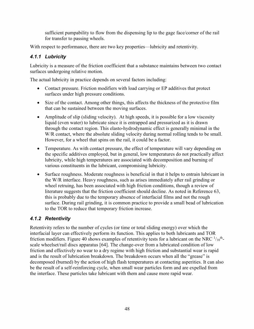
48
sufficient pumpability to flow from the dispensing lip to the gage face/corner of the rail for transfer to passing wheels.
With respect to performance, there are two key properties—lubricity and retentivity.
4.1.1 Lubricity
Lubricity is a measure of the friction coefficient that a substance maintains between two contact surfaces undergoing relative motion.
The actual lubricity in practice depends on several factors including:
• Contact pressure. Friction modifiers with load carrying or EP additives that protect surfaces under high pressure conditions.
• Size of the contact. Among other things, this affects the thickness of the protective film that can be sustained between the moving surfaces.
• Amplitude of slip (sliding velocity). At high speeds, it is possible for a low viscosity liquid (even water) to lubricate since it is entrapped and pressurized as it is drawn through the contact region. This elasto-hydrodynamic effect is generally minimal in the W/R contact, where the absolute sliding velocity during normal rolling tends to be small. However, for a wheel that spins on the rail, it could be a factor.
• Temperature. As with contact pressure, the effect of temperature will vary depending on the specific additives employed, but in general, low temperatures do not practically affect lubricity, while high temperatures are associated with decomposition and burning of various constituents in the lubricant, compromising lubricity.
• Surface roughness. Moderate roughness is beneficial in that it helps to entrain lubricant in the W/R interface. Heavy roughness, such as arises immediately after rail grinding or wheel retruing, has been associated with high friction conditions, though a review of literature suggests that the friction coefficient should decline. As noted in Reference 63, this is probably due to the temporary absence of interfacial films and not the rough surface. During rail grinding, it is common practice to provide a small bead of lubrication to the TOR to reduce that temporary friction increase.
4.1.2 Retentivity
Retentivity refers to the number of cycles (or time or total sliding energy) over which the interfacial layer can effectively perform its function. This applies to both lubricants and TOR friction modifiers. Figure 40 shows examples of retentivity tests for a lubricant on the NRC 1/10
th-scale wheelset/rail discs apparatus [64]. The change-over from a lubricated condition of low friction and effectively no wear to a dry regime with high friction and substantial wear is rapid and is the result of lubrication breakdown. The breakdown occurs when all the “grease” is decomposed (burned) by the action of high flash temperatures at contacting asperities. It can also be the result of a self-reinforcing cycle, when small wear particles form and are expelled from the interface. These particles take lubricant with them and cause more rapid wear.
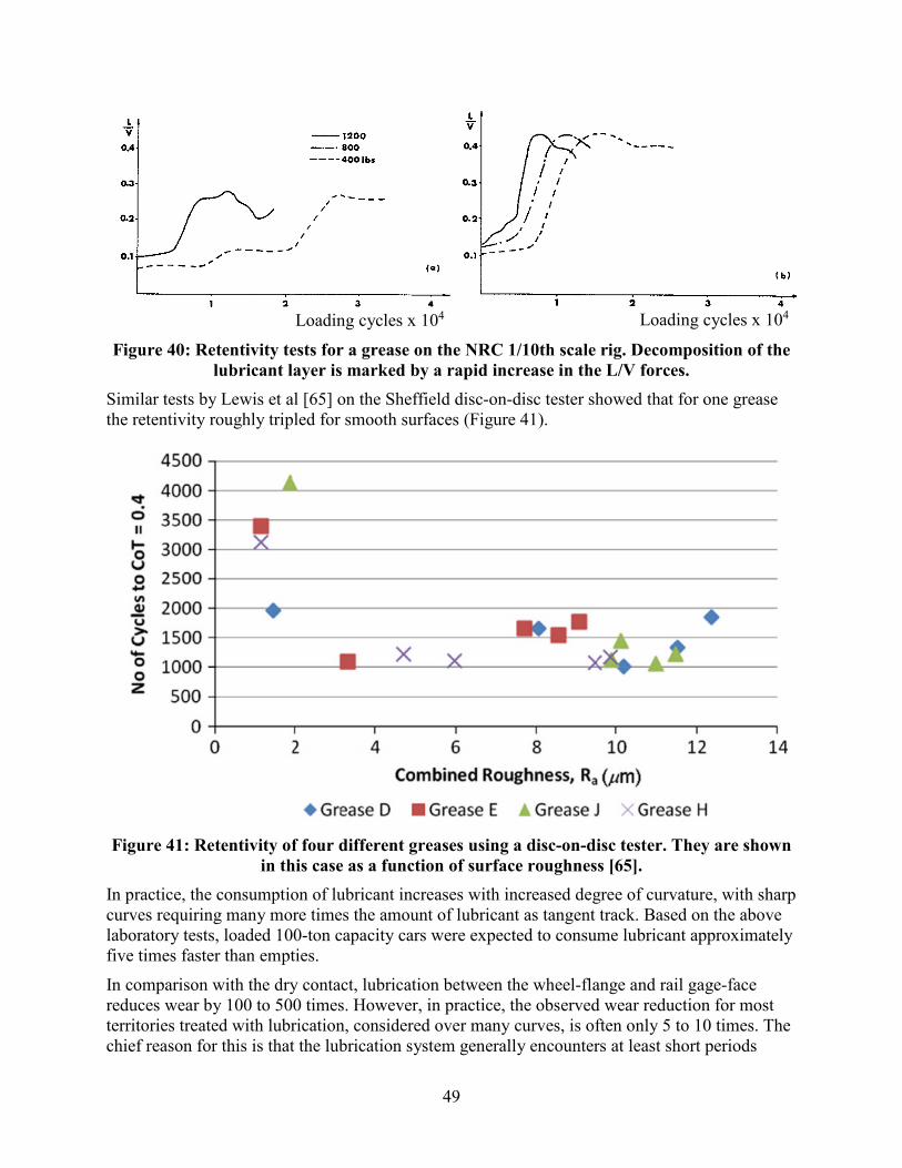
49
Loading cycles x 104
Loading cycles x 104
Figure 40: Retentivity tests for a grease on the NRC 1/10th scale rig. Decomposition of the lubricant layer is marked by a rapid increase in the L/V forces.
Similar tests by Lewis et al [65] on the Sheffield disc-on-disc tester showed that for one grease the retentivity roughly tripled for smooth surfaces (Figure 41).
Figure 41: Retentivity of four different greases using a disc-on-disc tester. They are shown
in this case as a function of surface roughness [65]. In practice, the consumption of lubricant increases with increased degree of curvature, with sharp curves requiring many more times the amount of lubricant as tangent track. Based on the above laboratory tests, loaded 100-ton capacity cars were expected to consume lubricant approximately five times faster than empties.
In comparison with the dry contact, lubrication between the wheel-flange and rail gage-face reduces wear by 100 to 500 times. However, in practice, the observed wear reduction for most territories treated with lubrication, considered over many curves, is often only 5 to 10 times. The chief reason for this is that the lubrication system generally encounters at least short periods
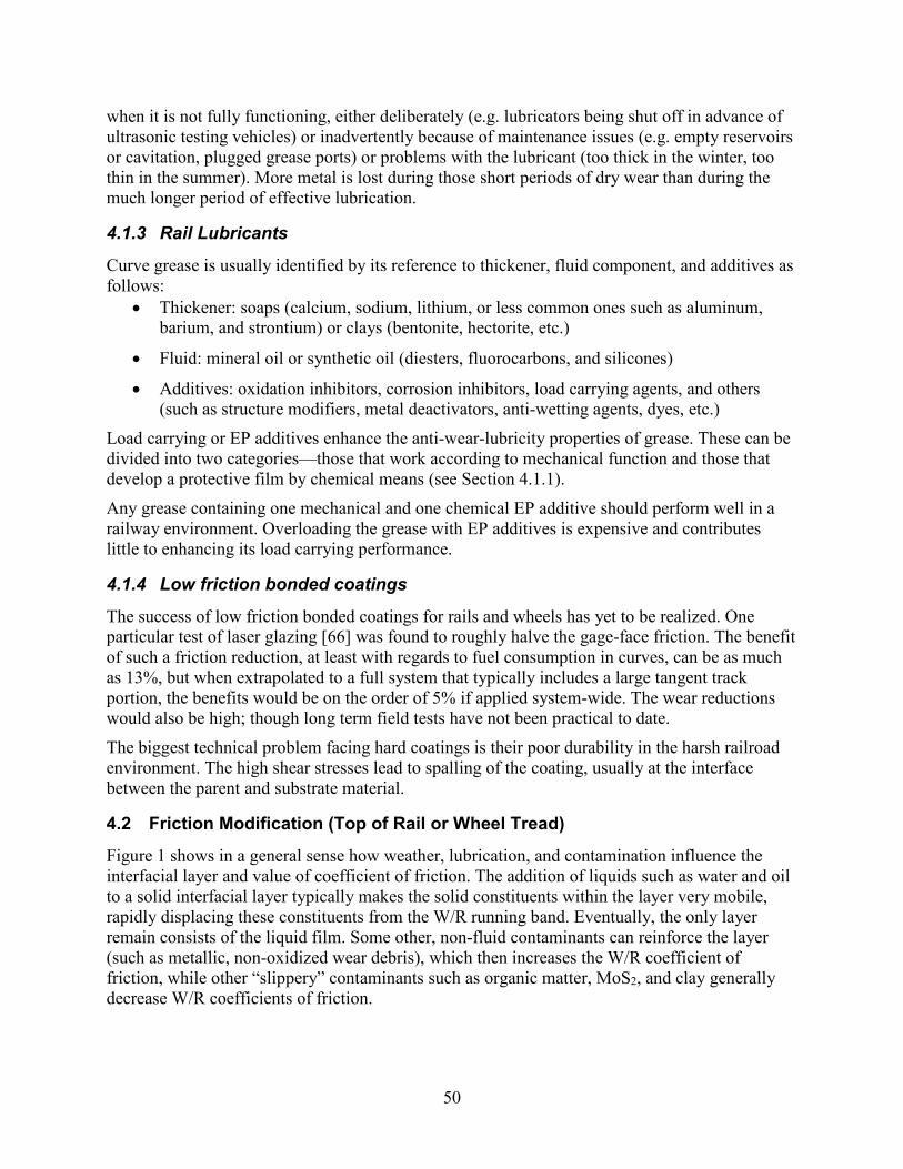
50
when it is not fully functioning, either deliberately (e.g. lubricators being shut off in advance of ultrasonic testing vehicles) or inadvertently because of maintenance issues (e.g. empty reservoirs or cavitation, plugged grease ports) or problems with the lubricant (too thick in the winter, too thin in the summer). More metal is lost during those short periods of dry wear than during the much longer period of effective lubrication.
4.1.3 Rail Lubricants
Curve grease is usually identified by its reference to thickener, fluid component, and additives as follows:
• Thickener: soaps (calcium, sodium, lithium, or less common ones such as aluminum, barium, and strontium) or clays (bentonite, hectorite, etc.)
• Fluid: mineral oil or synthetic oil (diesters, fluorocarbons, and silicones)
• Additives: oxidation inhibitors, corrosion inhibitors, load carrying agents, and others (such as structure modifiers, metal deactivators, anti-wetting agents, dyes, etc.)
Load carrying or EP additives enhance the anti-wear-lubricity properties of grease. These can be divided into two categories—those that work according to mechanical function and those that develop a protective film by chemical means (see Section 4.1.1).
Any grease containing one mechanical and one chemical EP additive should perform well in a railway environment. Overloading the grease with EP additives is expensive and contributes little to enhancing its load carrying performance.
4.1.4 Low friction bonded coatings
The success of low friction bonded coatings for rails and wheels has yet to be realized. One particular test of laser glazing [66] was found to roughly halve the gage-face friction. The benefit of such a friction reduction, at least with regards to fuel consumption in curves, can be as much as 13%, but when extrapolated to a full system that typically includes a large tangent track portion, the benefits would be on the order of 5% if applied system-wide. The wear reductions would also be high; though long term field tests have not been practical to date.
The biggest technical problem facing hard coatings is their poor durability in the harsh railroad environment. The high shear stresses lead to spalling of the coating, usually at the interface between the parent and substrate material.
4.2 Friction Modification (Top of Rail or Wheel Tread)
Figure 1 shows in a general sense how weather, lubrication, and contamination influence the interfacial layer and value of coefficient of friction. The addition of liquids such as water and oil to a solid interfacial layer typically makes the solid constituents within the layer very mobile, rapidly displacing these constituents from the W/R running band. Eventually, the only layer remain consists of the liquid film. Some other, non-fluid contaminants can reinforce the layer (such as metallic, non-oxidized wear debris), which then increases the W/R coefficient of friction, while other “slippery” contaminants such as organic matter, MoS2, and clay generally decrease W/R coefficients of friction.

51
The goal of a friction modifier that would work at the top-of-rail/wheel-tread interface is to provide an intermediate friction level, typically about 0.3-0.35. Thus, it is not a lubricant, but rather a mixture of solids and carriers that controls friction to the desired level.
A second important property of the friction modifier to consider is the traction-creep characteristic as discussed in Section 2.4. Some modifiers, such as sand, are known to have strong negative creep characteristics beyond the saturation point that contribute to noise, corrugation, and traction control difficulties. Natural items like grain mush and wood chips, in very modest quantities, can also provide a favorable top-of-rail friction condition. Some products are specifically engineered to provide a stable or positive traction-creepage characteristic.
4.2.1 Friction Modifiers
Friction modifiers come in two general forms: solid sticks that rub against the wheel running surface (Figure 42, left), or wayside systems that dispense a liquid product onto the rail running band (Figure 42, right). Both have been demonstrated to be quite effective in reducing wheel noise and vibration [67], reducing lateral forces [68, 47] and greenhouse gases [69], and to alleviate the growth of short pitch corrugations on mass transit lines [70, 71]. Other options for applying top-of-rail products are to use a manual roller or brush, or to spray the product with a hi-rail vehicle [72].
HPFTM sticks mounted against the wheel tread control noise and corrugation
A wayside application of KELTRACK® to the top of rail.
Figure 42: Controlling friction between the top of rail and wheel tread (photos courtesy of LBFoster).
Two other examples of engineered friction modifiers are shown in Figure 43. The second is a mixture of sand and stainless steel particles that are combined with an inorganic gelling agent, a stabilizer, and water. The gelling agent helps to flow and adhere the mixture to the rail and wheel surfaces while the stainless steel particles assure good electrical conductivity. This product has been used in the Netherlands since 1998.
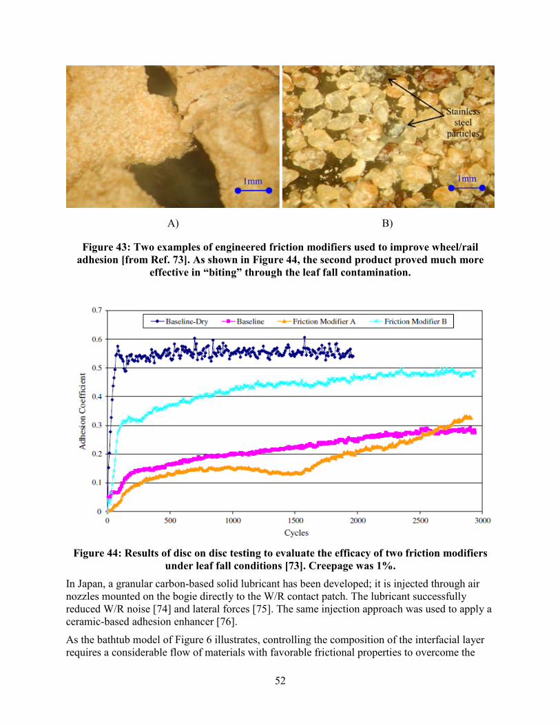
52
A) B)
Figure 43: Two examples of engineered friction modifiers used to improve wheel/rail adhesion [from Ref. 73]. As shown in Figure 44, the second product proved much more
effective in “biting” through the leaf fall contamination.
Figure 44: Results of disc on disc testing to evaluate the efficacy of two friction modifiers
under leaf fall conditions [73]. Creepage was 1%. In Japan, a granular carbon-based solid lubricant has been developed; it is injected through air nozzles mounted on the bogie directly to the W/R contact patch. The lubricant successfully reduced W/R noise [74] and lateral forces [75]. The same injection approach was used to apply a ceramic-based adhesion enhancer [76].
As the bathtub model of Figure 6 illustrates, controlling the composition of the interfacial layer requires a considerable flow of materials with favorable frictional properties to overcome the
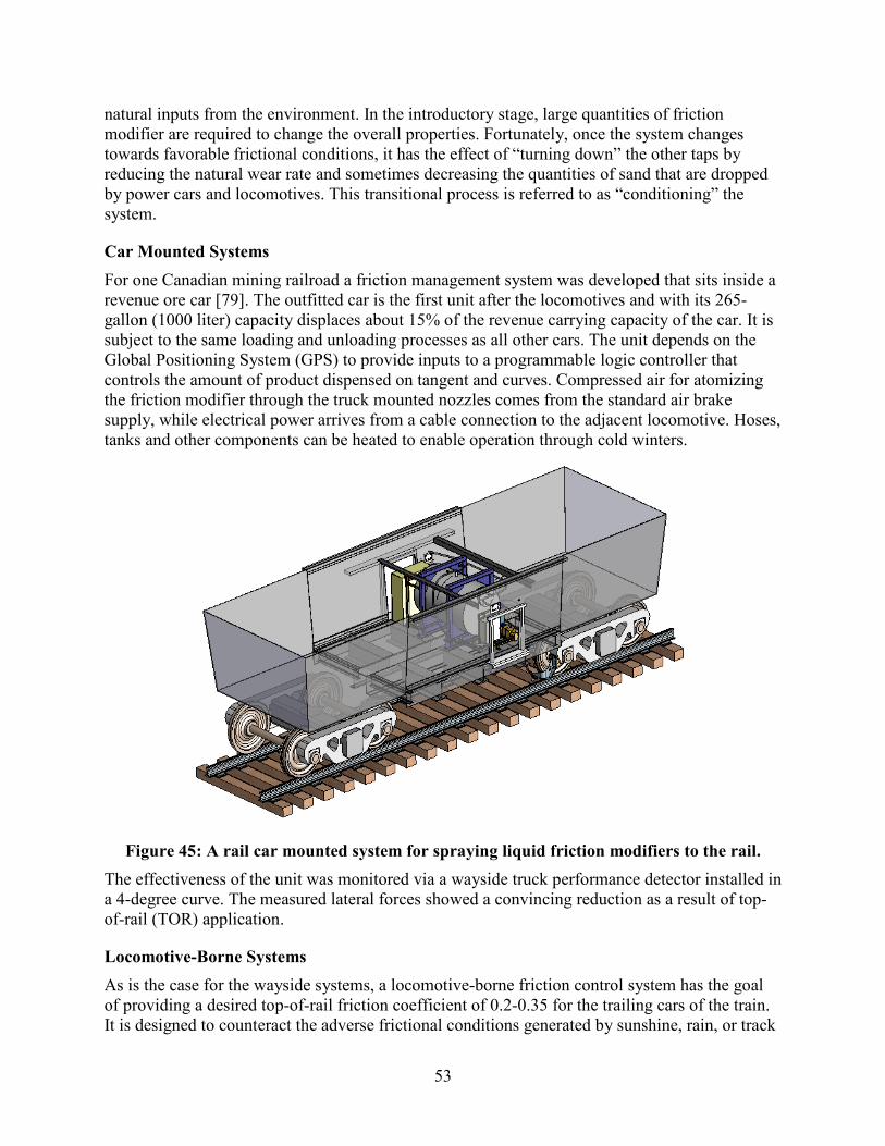
53
natural inputs from the environment. In the introductory stage, large quantities of friction modifier are required to change the overall properties. Fortunately, once the system changes towards favorable frictional conditions, it has the effect of “turning down” the other taps by reducing the natural wear rate and sometimes decreasing the quantities of sand that are dropped by power cars and locomotives. This transitional process is referred to as “conditioning” the system.
Car Mounted Systems For one Canadian mining railroad a friction management system was developed that sits inside a revenue ore car [79]. The outfitted car is the first unit after the locomotives and with its 265-gallon (1000 liter) capacity displaces about 15% of the revenue carrying capacity of the car. It is subject to the same loading and unloading processes as all other cars. The unit depends on the Global Positioning System (GPS) to provide inputs to a programmable logic controller that controls the amount of product dispensed on tangent and curves. Compressed air for atomizing the friction modifier through the truck mounted nozzles comes from the standard air brake supply, while electrical power arrives from a cable connection to the adjacent locomotive. Hoses, tanks and other components can be heated to enable operation through cold winters.
Figure 45: A rail car mounted system for spraying liquid friction modifiers to the rail.
The effectiveness of the unit was monitored via a wayside truck performance detector installed in a 4-degree curve. The measured lateral forces showed a convincing reduction as a result of top-of-rail (TOR) application.
Locomotive-Borne Systems As is the case for the wayside systems, a locomotive-borne friction control system has the goal of providing a desired top-of-rail friction coefficient of 0.2-0.35 for the trailing cars of the train. It is designed to counteract the adverse frictional conditions generated by sunshine, rain, or track
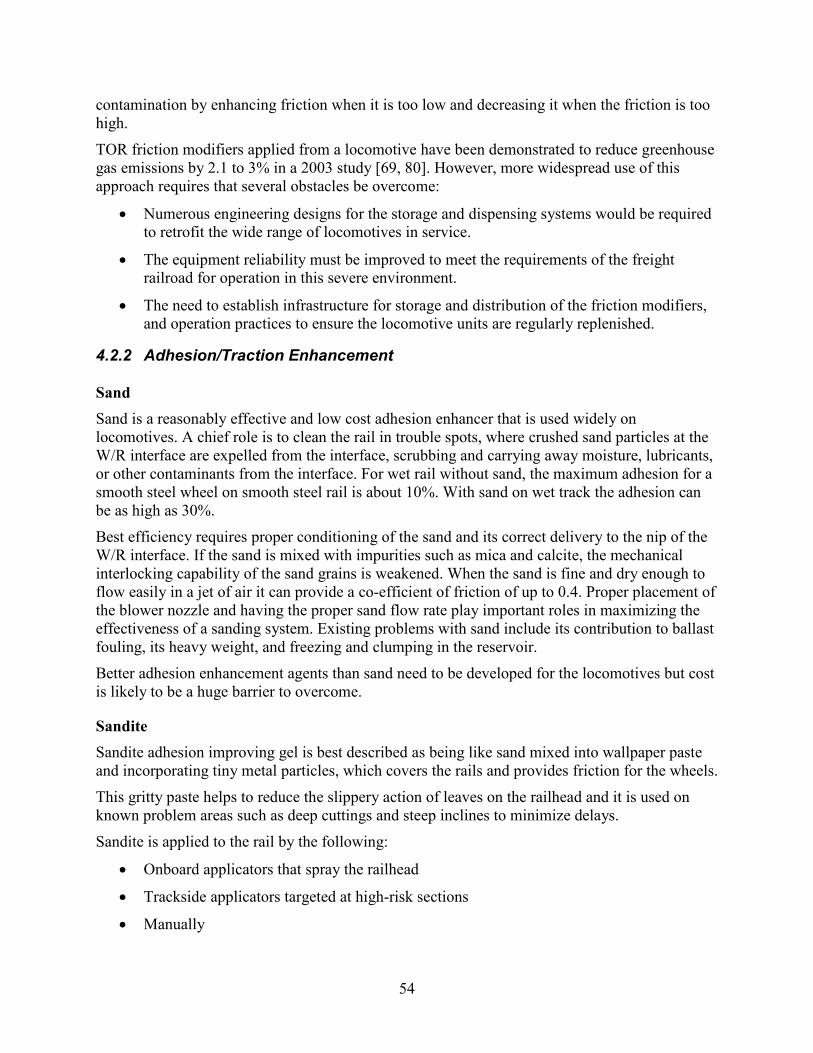
54
contamination by enhancing friction when it is too low and decreasing it when the friction is too high.
TOR friction modifiers applied from a locomotive have been demonstrated to reduce greenhouse gas emissions by 2.1 to 3% in a 2003 study [69, 80]. However, more widespread use of this approach requires that several obstacles be overcome:
• Numerous engineering designs for the storage and dispensing systems would be required to retrofit the wide range of locomotives in service.
• The equipment reliability must be improved to meet the requirements of the freight railroad for operation in this severe environment.
• The need to establish infrastructure for storage and distribution of the friction modifiers, and operation practices to ensure the locomotive units are regularly replenished.
4.2.2 Adhesion/Traction Enhancement
Sand Sand is a reasonably effective and low cost adhesion enhancer that is used widely on locomotives. A chief role is to clean the rail in trouble spots, where crushed sand particles at the W/R interface are expelled from the interface, scrubbing and carrying away moisture, lubricants, or other contaminants from the interface. For wet rail without sand, the maximum adhesion for a smooth steel wheel on smooth steel rail is about 10%. With sand on wet track the adhesion can be as high as 30%.
Best efficiency requires proper conditioning of the sand and its correct delivery to the nip of the W/R interface. If the sand is mixed with impurities such as mica and calcite, the mechanical interlocking capability of the sand grains is weakened. When the sand is fine and dry enough to flow easily in a jet of air it can provide a co-efficient of friction of up to 0.4. Proper placement of the blower nozzle and having the proper sand flow rate play important roles in maximizing the effectiveness of a sanding system. Existing problems with sand include its contribution to ballast fouling, its heavy weight, and freezing and clumping in the reservoir.
Better adhesion enhancement agents than sand need to be developed for the locomotives but cost is likely to be a huge barrier to overcome.
Sandite Sandite adhesion improving gel is best described as being like sand mixed into wallpaper paste and incorporating tiny metal particles, which covers the rails and provides friction for the wheels.
This gritty paste helps to reduce the slippery action of leaves on the railhead and it is used on known problem areas such as deep cuttings and steep inclines to minimize delays.
Sandite is applied to the rail by the following:
• Onboard applicators that spray the railhead
• Trackside applicators targeted at high-risk sections
• Manually
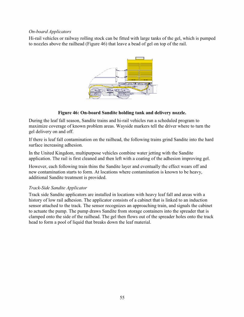
55
On-board Applicators Hi-rail vehicles or railway rolling stock can be fitted with large tanks of the gel, which is pumped to nozzles above the railhead (Figure 46) that leave a bead of gel on top of the rail.
Figure 46: On-board Sandite holding tank and delivery nozzle. During the leaf fall season, Sandite trains and hi-rail vehicles run a scheduled program to maximize coverage of known problem areas. Wayside markers tell the driver where to turn the gel delivery on and off.
If there is leaf fall contamination on the railhead, the following trains grind Sandite into the hard surface increasing adhesion.
In the United Kingdom, multipurpose vehicles combine water jetting with the Sandite application. The rail is first cleaned and then left with a coating of the adhesion improving gel.
However, each following train thins the Sandite layer and eventually the effect wears off and new contamination starts to form. At locations where contamination is known to be heavy, additional Sandite treatment is provided.
Track-Side Sandite Applicator Track side Sandite applicators are installed in locations with heavy leaf fall and areas with a history of low rail adhesion. The applicator consists of a cabinet that is linked to an induction sensor attached to the track. The sensor recognizes an approaching train, and signals the cabinet to actuate the pump. The pump draws Sandite from storage containers into the spreader that is clamped onto the side of the railhead. The gel then flows out of the spreader holes onto the track head to form a pool of liquid that breaks down the leaf material.
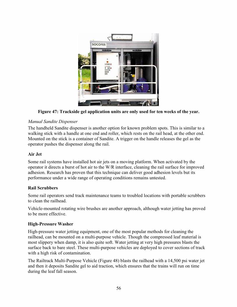
56
Figure 47: Trackside gel application units are only used for ten weeks of the year.
Manual Sandite Dispenser The handheld Sandite dispenser is another option for known problem spots. This is similar to a walking stick with a handle at one end and roller, which rests on the rail head, at the other end. Mounted on the stick is a container of Sandite. A trigger on the handle releases the gel as the operator pushes the dispenser along the rail.
Air Jet Some rail systems have installed hot air jets on a moving platform. When activated by the operator it directs a burst of hot air to the W/R interface, cleaning the rail surface for improved adhesion. Research has proven that this technique can deliver good adhesion levels but its performance under a wide range of operating conditions remains untested.
Rail Scrubbers Some rail operators send track maintenance teams to troubled locations with portable scrubbers to clean the railhead.
Vehicle-mounted rotating wire brushes are another approach, although water jetting has proved to be more effective.
High-Pressure Washer High-pressure water jetting equipment, one of the most popular methods for cleaning the railhead, can be mounted on a multi-purpose vehicle. Though the compressed leaf material is most slippery when damp, it is also quite soft. Water jetting at very high pressures blasts the surface back to bare steel. These multi-purpose vehicles are deployed to cover sections of track with a high risk of contamination.
The Railtrack Multi-Purpose Vehicle (Figure 48) blasts the railhead with a 14,500 psi water jet and then it deposits Sandite gel to aid traction, which ensures that the trains will run on time during the leaf fall season.
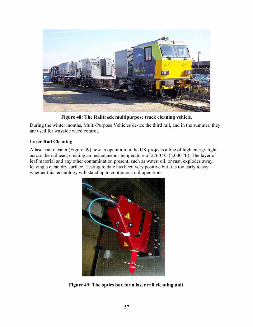
57
Figure 48: The Railtrack multipurpose track cleaning vehicle.
During the winter months, Multi-Purpose Vehicles de-ice the third rail, and in the summer, they are used for wayside weed control.
Laser Rail Cleaning A laser rail cleaner (Figure 49) now in operation in the UK projects a line of high energy light across the railhead, creating an instantaneous temperature of 2760 °C (5,000 °F). The layer of leaf material and any other contamination present, such as water, oil, or rust, explodes away, leaving a clean dry surface. Testing to date has been very positive but it is too early to say whether this technology will stand up to continuous rail operations.
Figure 49: The optics box for a laser rail cleaning unit.
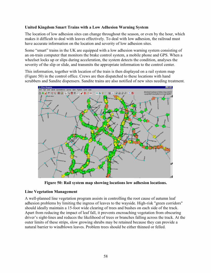
58
United Kingdom Smart Trains with a Low Adhesion Warning System The location of low adhesion sites can change throughout the season, or even by the hour, which makes it difficult to deal with leaves effectively. To deal with low adhesion, the railroad must have accurate information on the location and severity of low adhesion sites.
Some “smart” trains in the UK are equipped with a low adhesion warning system consisting of an on-train computer that monitors the brake control system, a mobile phone and GPS. When a wheelset locks up or slips during acceleration, the system detects the condition, analyses the severity of the slip or slide, and transmits the appropriate information to the control center.
This information, together with location of the train is then displayed on a rail system map (Figure 50) in the control office. Crews are then dispatched to these locations with hand scrubbers and Sandite dispensers. Sandite trains are also notified of new sites needing treatment.
Figure 50: Rail system map showing locations low adhesion locations.
Line Vegetation Management A well-planned line vegetation program assists in controlling the root cause of autumn leaf adhesion problems by limiting the ingress of leaves to the wayside. High-risk "green corridors" should ideally maintain a 15-foot wide clearing of trees and bushes on each side of the track. Apart from reducing the impact of leaf fall, it prevents encroaching vegetation from obscuring driver’s sight-lines and reduces the likelihood of trees or branches falling across the track. At the outer limits of these strips, slow growing shrubs may be retained because they can provide a natural barrier to windblown leaves. Problem trees should be either thinned or felled.
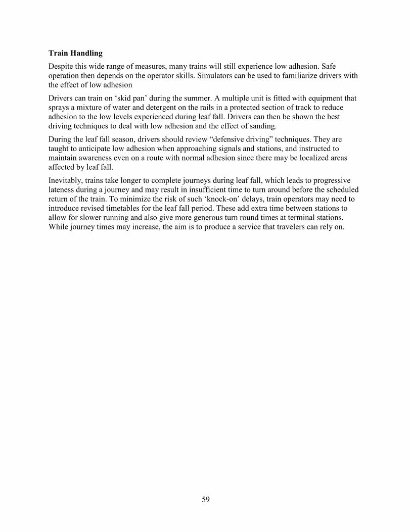
59
Train Handling Despite this wide range of measures, many trains will still experience low adhesion. Safe operation then depends on the operator skills. Simulators can be used to familiarize drivers with the effect of low adhesion
Drivers can train on ‘skid pan’ during the summer. A multiple unit is fitted with equipment that sprays a mixture of water and detergent on the rails in a protected section of track to reduce adhesion to the low levels experienced during leaf fall. Drivers can then be shown the best driving techniques to deal with low adhesion and the effect of sanding.
During the leaf fall season, drivers should review “defensive driving” techniques. They are taught to anticipate low adhesion when approaching signals and stations, and instructed to maintain awareness even on a route with normal adhesion since there may be localized areas affected by leaf fall.
Inevitably, trains take longer to complete journeys during leaf fall, which leads to progressive lateness during a journey and may result in insufficient time to turn around before the scheduled return of the train. To minimize the risk of such ‘knock-on’ delays, train operators may need to introduce revised timetables for the leaf fall period. These add extra time between stations to allow for slower running and also give more generous turn round times at terminal stations. While journey times may increase, the aim is to produce a service that travelers can rely on.

60
5. Methods for Measuring Friction
5.1 Laboratory-Scale Systems
Laboratory-scale systems are designed and intended to remain in a clean space with controlled levels of contamination. Most often they use small samples cut from the larger bodies, such that the contact conditions need to be scaled to represent the “real world” conditions. The laboratory instruments, with simple and well understood geometries under well-controlled conditions, are valuable for gaining fundamental understandings around friction. Typically, it is difficult to scale laboratory measurements to full scale systems.
5.1.1 The Friction Force Microscope
Scanning tunnel microscopy involves the movement of a very tiny cantilevered arm across a surface, with its deflections being measured with lasers [24]. This allows measurements of topography and friction at the nano-scale. As this is of little relevance to the mesoscopic W/R contact, we will leave the description there.
5.1.2 Pin-on-disc
The pin-on-disc rigs employ a rigid pin, mounted in an instrumented assembly that allows the force applied to the pin to be monitored. Vertical load is typically applied with dead weights. The geometry on the pin can be spherical, cylindrical, or others. Most commonly, the pin is stationary while the disc rotates underneath. Under these conditions, the peak traction is a measure of the friction coefficient under those conditions.
Figure 51: Pin-on-disc rig (Fig. 4.2 of Ref [33].
Compared with other friction testing methods, the pin-on-disc rig has the advantage of requiring only small test samples and testing is relatively affordable. Its main disadvantage is that the test conditions poorly replicate the W/R contact, but might be applicable to other railway systems such as at constant contact side bearings, the friction wedge and pocket, and the brake beam slide.
Powder Rheometer The National Research Council (NRC) of Canada applied the pin-on-disc principle to create a powder rheometer. It applies a dead weight through a lever arm against two stationary pins that contact a rotating anvil that is coated with a powder layer (Figure 52). A numerically-controlled
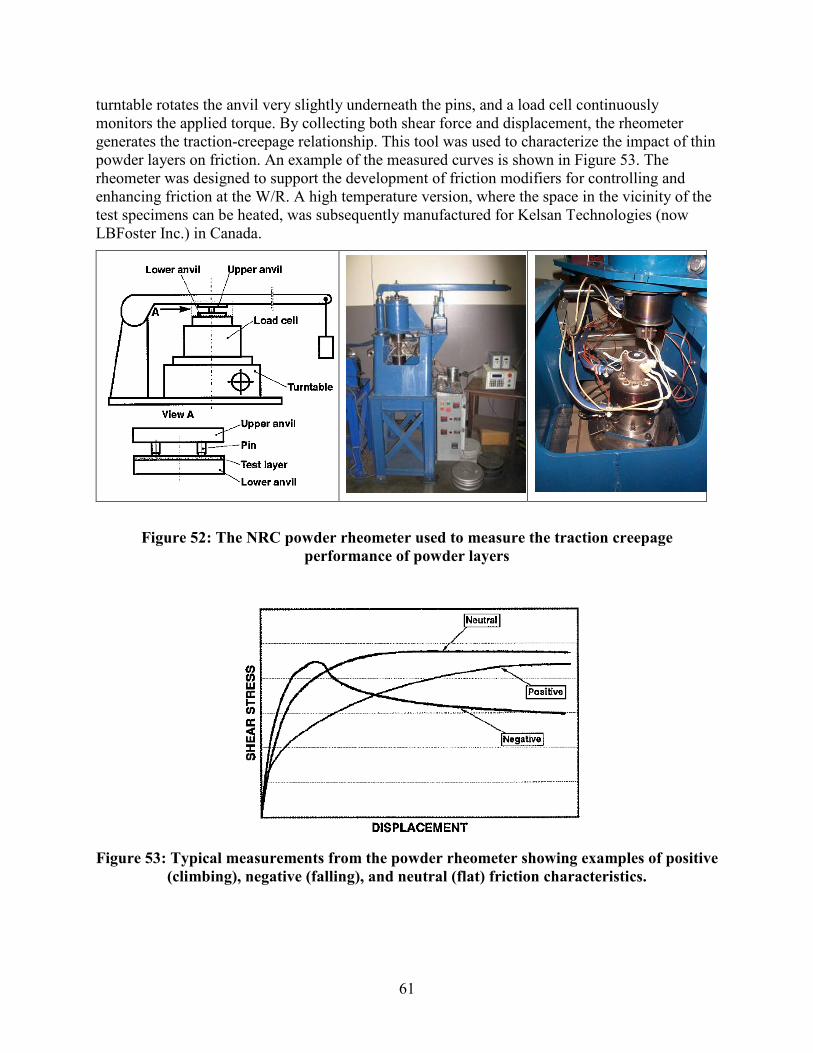
61
turntable rotates the anvil very slightly underneath the pins, and a load cell continuously monitors the applied torque. By collecting both shear force and displacement, the rheometer generates the traction-creepage relationship. This tool was used to characterize the impact of thin powder layers on friction. An example of the measured curves is shown in Figure 53. The rheometer was designed to support the development of friction modifiers for controlling and enhancing friction at the W/R. A high temperature version, where the space in the vicinity of the test specimens can be heated, was subsequently manufactured for Kelsan Technologies (now LBFoster Inc.) in Canada.
Figure 52: The NRC powder rheometer used to measure the traction creepage performance of powder layers
Figure 53: Typical measurements from the powder rheometer showing examples of positive
(climbing), negative (falling), and neutral (flat) friction characteristics.
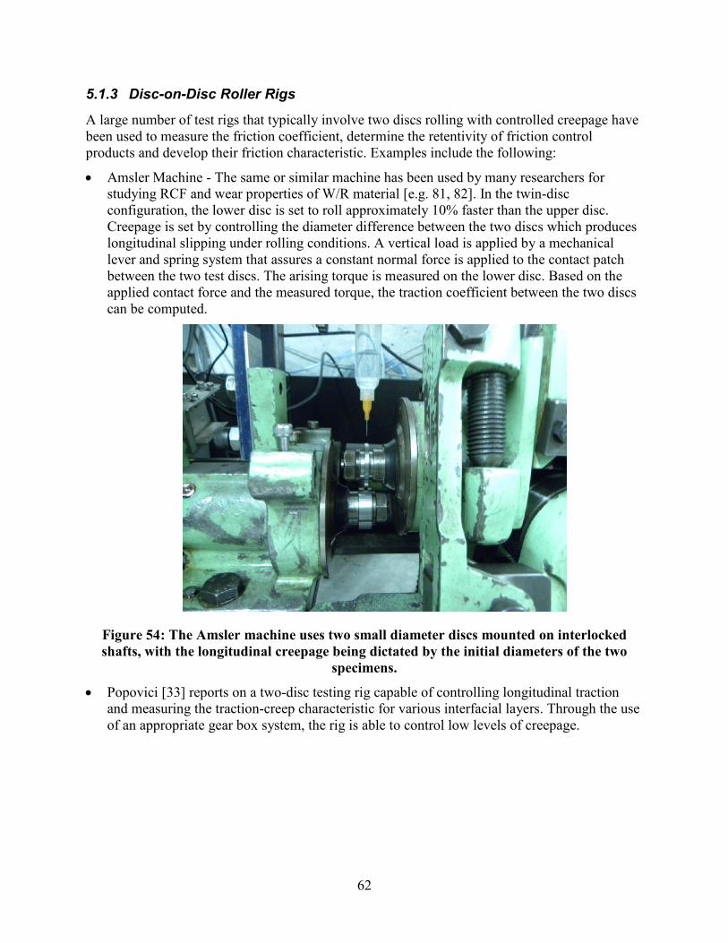
62
5.1.3 Disc-on-Disc Roller Rigs
A large number of test rigs that typically involve two discs rolling with controlled creepage have been used to measure the friction coefficient, determine the retentivity of friction control products and develop their friction characteristic. Examples include the following:
• Amsler Machine - The same or similar machine has been used by many researchers for studying RCF and wear properties of W/R material [e.g. 81, 82]. In the twin-disc configuration, the lower disc is set to roll approximately 10% faster than the upper disc. Creepage is set by controlling the diameter difference between the two discs which produces longitudinal slipping under rolling conditions. A vertical load is applied by a mechanical lever and spring system that assures a constant normal force is applied to the contact patch between the two test discs. The arising torque is measured on the lower disc. Based on the applied contact force and the measured torque, the traction coefficient between the two discs can be computed.
Figure 54: The Amsler machine uses two small diameter discs mounted on interlocked shafts, with the longitudinal creepage being dictated by the initial diameters of the two
specimens.
• Popovici [33] reports on a two-disc testing rig capable of controlling longitudinal traction and measuring the traction-creep characteristic for various interfacial layers. Through the use of an appropriate gear box system, the rig is able to control low levels of creepage.
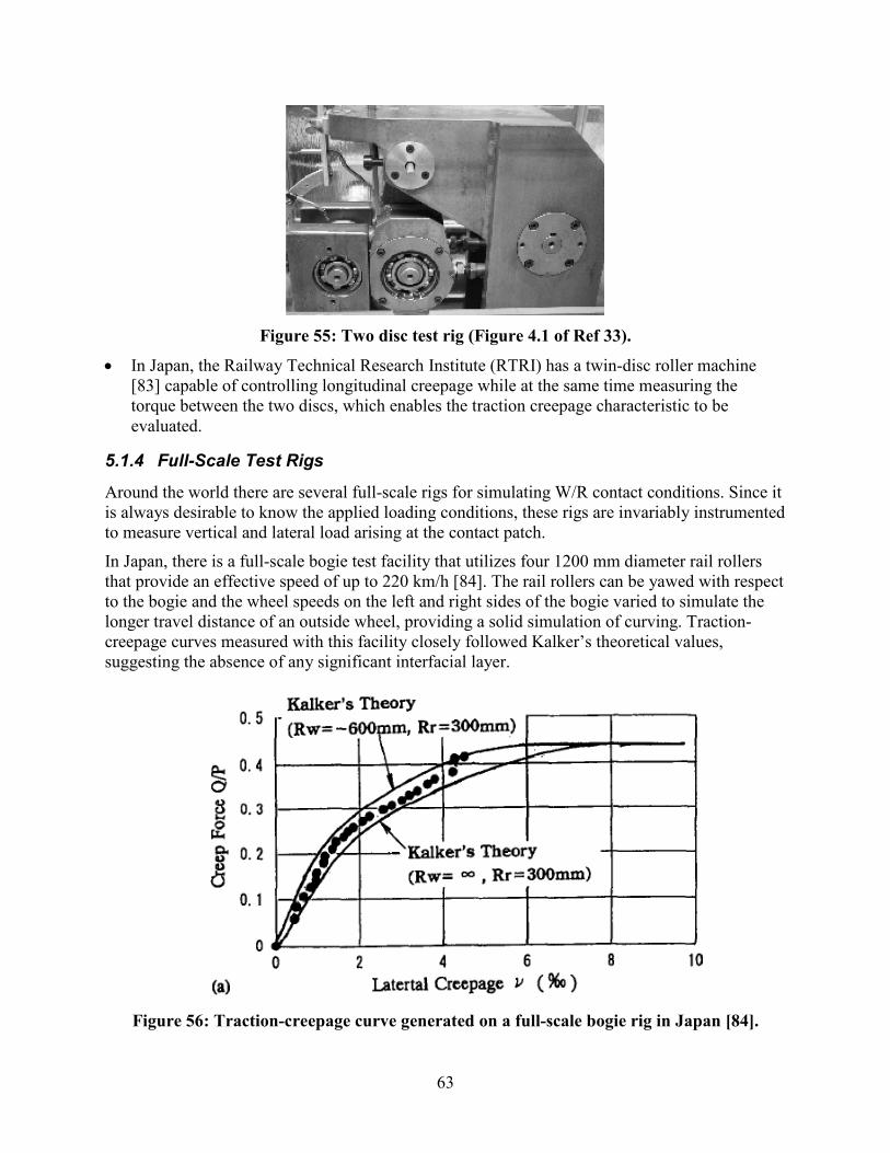
63
Figure 55: Two disc test rig (Figure 4.1 of Ref 33).
• In Japan, the Railway Technical Research Institute (RTRI) has a twin-disc roller machine [83] capable of controlling longitudinal creepage while at the same time measuring the torque between the two discs, which enables the traction creepage characteristic to be evaluated.
5.1.4 Full-Scale Test Rigs
Around the world there are several full-scale rigs for simulating W/R contact conditions. Since it is always desirable to know the applied loading conditions, these rigs are invariably instrumented to measure vertical and lateral load arising at the contact patch.
In Japan, there is a full-scale bogie test facility that utilizes four 1200 mm diameter rail rollers that provide an effective speed of up to 220 km/h [84]. The rail rollers can be yawed with respect to the bogie and the wheel speeds on the left and right sides of the bogie varied to simulate the longer travel distance of an outside wheel, providing a solid simulation of curving. Traction-creepage curves measured with this facility closely followed Kalker’s theoretical values, suggesting the absence of any significant interfacial layer.
Figure 56: Traction-creepage curve generated on a full-scale bogie rig in Japan [84].
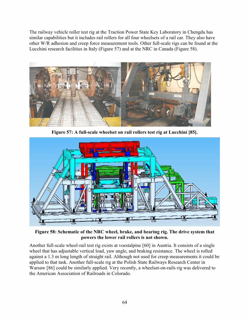
64
The railway vehicle roller test rig at the Traction Power State Key Laboratory in Chengdu has similar capabilities but it includes rail rollers for all four wheelsets of a rail car. They also have other W/R adhesion and creep force measurement tools. Other full-scale rigs can be found at the Lucchini research facilities in Italy (Figure 57) and at the NRC in Canada (Figure 58).
Figure 57: A full-scale wheelset on rail rollers test rig at Lucchini [85].
Figure 58: Schematic of the NRC wheel, brake, and bearing rig. The drive system that
powers the lower rail rollers is not shown. Another full-scale wheel-rail test rig exists at voestalpine [60] in Austria. It consists of a single wheel that has adjustable vertical load, yaw angle, and braking resistance. The wheel is rolled against a 1.3 m long length of straight rail. Although not used for creep measurements it could be applied to that task. Another full-scale rig at the Polish State Railways Research Center in Warsaw [86] could be similarly applied. Very recently, a wheelset-on-rails rig was delivered to the American Association of Railroads in Colorado.
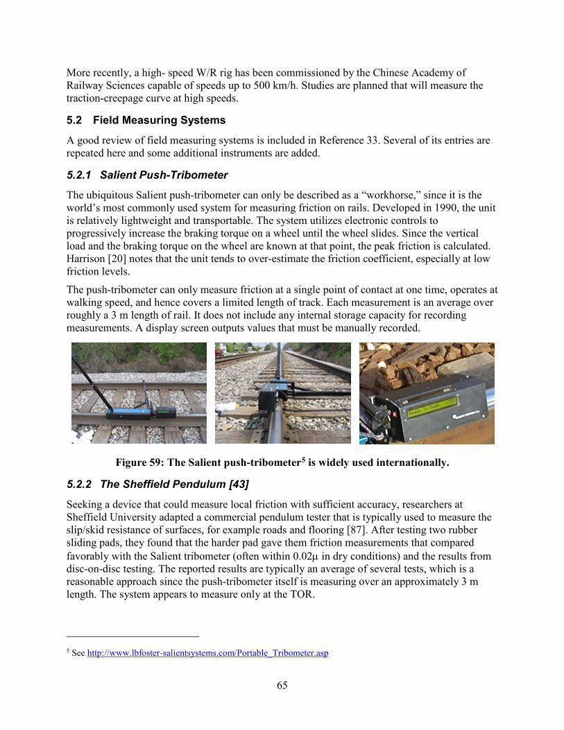
65
More recently, a high- speed W/R rig has been commissioned by the Chinese Academy of Railway Sciences capable of speeds up to 500 km/h. Studies are planned that will measure the traction-creepage curve at high speeds.
5.2 Field Measuring Systems
A good review of field measuring systems is included in Reference 33. Several of its entries are repeated here and some additional instruments are added.
5.2.1 Salient Push-Tribometer
The ubiquitous Salient push-tribometer can only be described as a “workhorse,” since it is the world’s most commonly used system for measuring friction on rails. Developed in 1990, the unit is relatively lightweight and transportable. The system utilizes electronic controls to progressively increase the braking torque on a wheel until the wheel slides. Since the vertical load and the braking torque on the wheel are known at that point, the peak friction is calculated. Harrison [20] notes that the unit tends to over-estimate the friction coefficient, especially at low friction levels.
The push-tribometer can only measure friction at a single point of contact at one time, operates at walking speed, and hence covers a limited length of track. Each measurement is an average over roughly a 3 m length of rail. It does not include any internal storage capacity for recording measurements. A display screen outputs values that must be manually recorded.
Figure 59: The Salient push-tribometer5 is widely used internationally.
5.2.2 The Sheffield Pendulum [43]
Seeking a device that could measure local friction with sufficient accuracy, researchers at Sheffield University adapted a commercial pendulum tester that is typically used to measure the slip/skid resistance of surfaces, for example roads and flooring [87]. After testing two rubber sliding pads, they found that the harder pad gave them friction measurements that compared favorably with the Salient tribometer (often within 0.02µ in dry conditions) and the results from disc-on-disc testing. The reported results are typically an average of several tests, which is a reasonable approach since the push-tribometer itself is measuring over an approximately 3 m length. The system appears to measure only at the TOR.
5 See http://www.lbfoster-salientsystems.com/Portable_Tribometer.asp
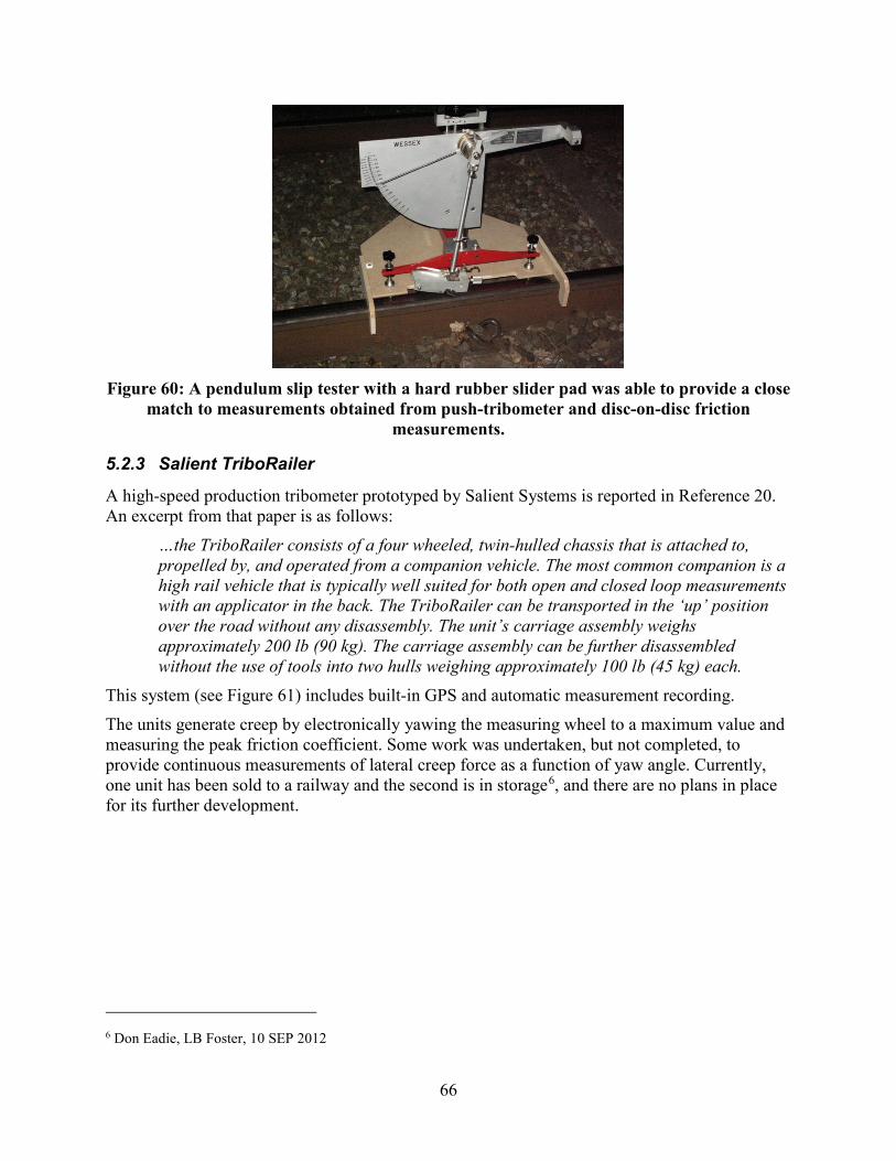
66
Figure 60: A pendulum slip tester with a hard rubber slider pad was able to provide a close
match to measurements obtained from push-tribometer and disc-on-disc friction measurements.
5.2.3 Salient TriboRailer
A high-speed production tribometer prototyped by Salient Systems is reported in Reference 20. An excerpt from that paper is as follows:
…the TriboRailer consists of a four wheeled, twin-hulled chassis that is attached to, propelled by, and operated from a companion vehicle. The most common companion is a high rail vehicle that is typically well suited for both open and closed loop measurements with an applicator in the back. The TriboRailer can be transported in the ‘up’ position over the road without any disassembly. The unit’s carriage assembly weighs approximately 200 lb (90 kg). The carriage assembly can be further disassembled without the use of tools into two hulls weighing approximately 100 lb (45 kg) each.
This system (see Figure 61) includes built-in GPS and automatic measurement recording.
The units generate creep by electronically yawing the measuring wheel to a maximum value and measuring the peak friction coefficient. Some work was undertaken, but not completed, to provide continuous measurements of lateral creep force as a function of yaw angle. Currently, one unit has been sold to a railway and the second is in storage6, and there are no plans in place for its further development.
6 Don Eadie, LB Foster, 10 SEP 2012
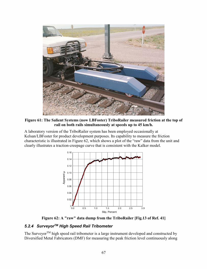
67
Figure 61: The Salient Systems (now LBFoster) TriboRailer measured friction at the top of
rail on both rails simultaneously at speeds up to 45 km/h. A laboratory version of the TriboRailer system has been employed occasionally at Kelsan/LBFoster for product development purposes. Its capability to measure the friction characteristic is illustrated in Figure 62, which shows a plot of the “raw” data from the unit and clearly illustrates a traction-creepage curve that is consistent with the Kalker model.
Figure 62: A "raw" data dump from the TriboRailer [Fig.13 of Ref. 41]
5.2.4 SurveyorTM High Speed Rail Tribometer
The SurveyorTM high speed rail tribometer is a large instrument developed and constructed by Diversified Metal Fabricators (DMF) for measuring the peak friction level continuously along
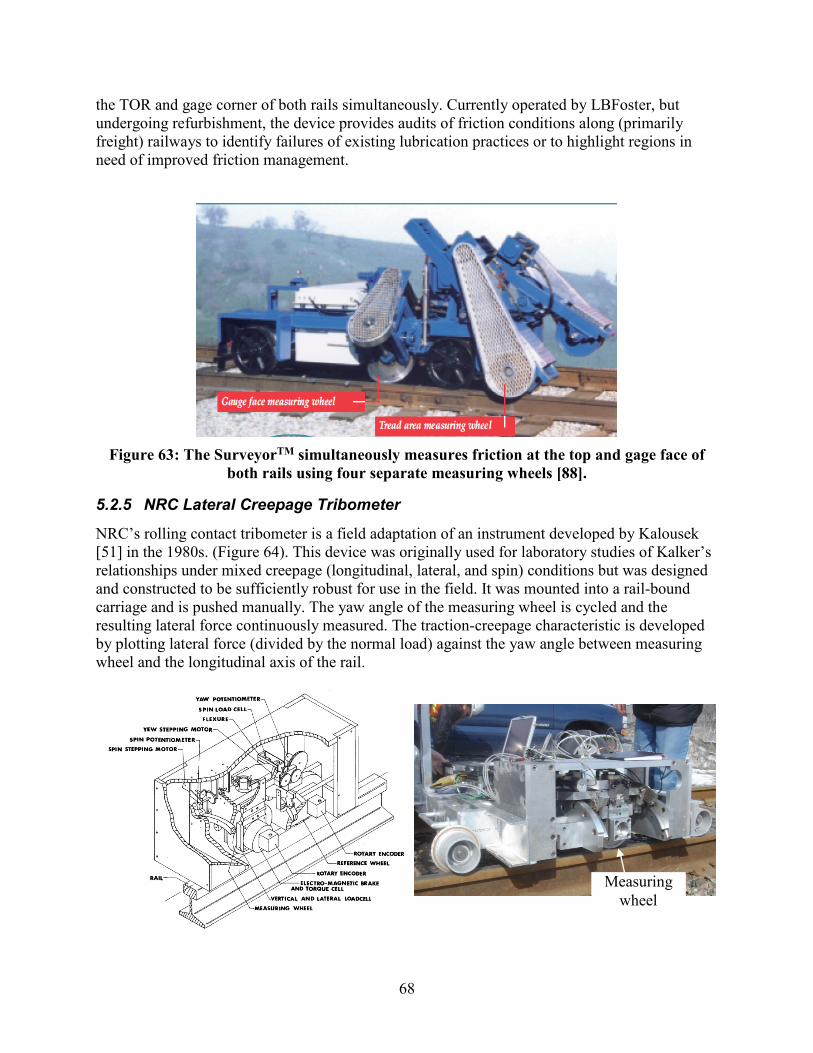
68
the TOR and gage corner of both rails simultaneously. Currently operated by LBFoster, but undergoing refurbishment, the device provides audits of friction conditions along (primarily freight) railways to identify failures of existing lubrication practices or to highlight regions in need of improved friction management.
Figure 63: The SurveyorTM simultaneously measures friction at the top and gage face of
both rails using four separate measuring wheels [88].
5.2.5 NRC Lateral Creepage Tribometer
NRC’s rolling contact tribometer is a field adaptation of an instrument developed by Kalousek [51] in the 1980s. (Figure 64). This device was originally used for laboratory studies of Kalker’s relationships under mixed creepage (longitudinal, lateral, and spin) conditions but was designed and constructed to be sufficiently robust for use in the field. It was mounted into a rail-bound carriage and is pushed manually. The yaw angle of the measuring wheel is cycled and the resulting lateral force continuously measured. The traction-creepage characteristic is developed by plotting lateral force (divided by the normal load) against the yaw angle between measuring wheel and the longitudinal axis of the rail.
Measuring wheel
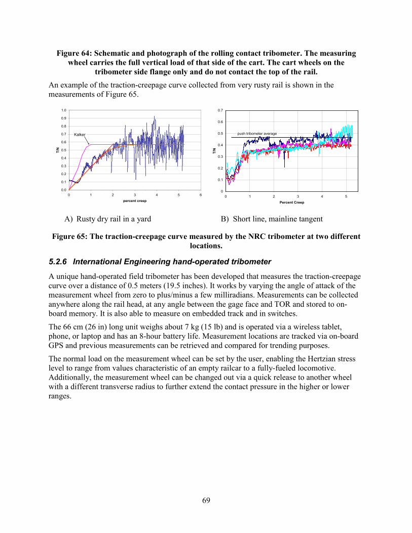
69
Figure 64: Schematic and photograph of the rolling contact tribometer. The measuring wheel carries the full vertical load of that side of the cart. The cart wheels on the
tribometer side flange only and do not contact the top of the rail. An example of the traction-creepage curve collected from very rusty rail is shown in the measurements of Figure 65.
A) Rusty dry rail in a yard B) Short line, mainline tangent
Figure 65: The traction-creepage curve measured by the NRC tribometer at two different locations.
5.2.6 International Engineering hand-operated tribometer
A unique hand-operated field tribometer has been developed that measures the traction-creepage curve over a distance of 0.5 meters (19.5 inches). It works by varying the angle of attack of the measurement wheel from zero to plus/minus a few milliradians. Measurements can be collected anywhere along the rail head, at any angle between the gage face and TOR and stored to on-board memory. It is also able to measure on embedded track and in switches.
The 66 cm (26 in) long unit weighs about 7 kg (15 lb) and is operated via a wireless tablet, phone, or laptop and has an 8-hour battery life. Measurement locations are tracked via on-board GPS and previous measurements can be retrieved and compared for trending purposes.
The normal load on the measurement wheel can be set by the user, enabling the Hertzian stress level to range from values characteristic of an empty railcar to a fully-fueled locomotive. Additionally, the measurement wheel can be changed out via a quick release to another wheel with a different transverse radius to further extend the contact pressure in the higher or lower ranges.
0.0
0.1
0.2
0.3
0.4
0.5
0.6
0.7
0.8
0.9
1.0
0 1 2 3 4 5 6
percent creep
T/N
Kalker
0
0.1
0.2
0.3
0.4
0.5
0.6
0.7
0 1 2 3 4 5
Percent Creep
T/N
push tribometer average
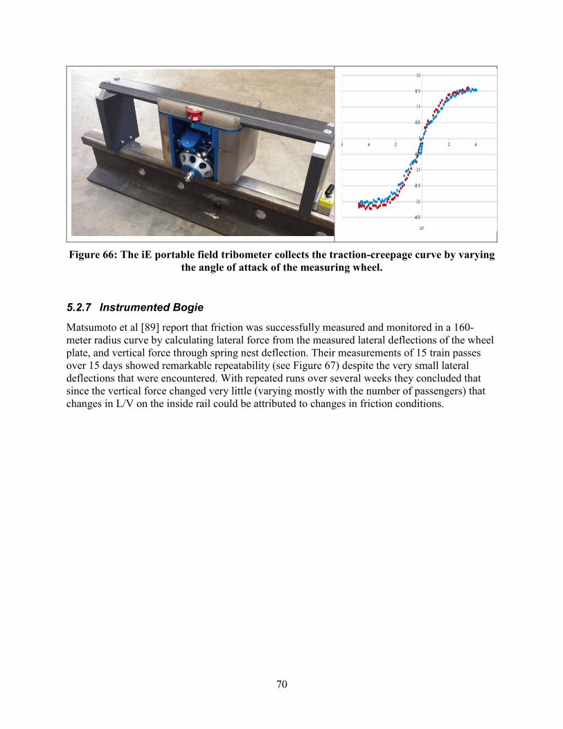
70
Figure 66: The iE portable field tribometer collects the traction-creepage curve by varying the angle of attack of the measuring wheel.
5.2.7 Instrumented Bogie
Matsumoto et al [89] report that friction was successfully measured and monitored in a 160-meter radius curve by calculating lateral force from the measured lateral deflections of the wheel plate, and vertical force through spring nest deflection. Their measurements of 15 train passes over 15 days showed remarkable repeatability (see Figure 67) despite the very small lateral deflections that were encountered. With repeated runs over several weeks they concluded that since the vertical force changed very little (varying mostly with the number of passengers) that changes in L/V on the inside rail could be attributed to changes in friction conditions.
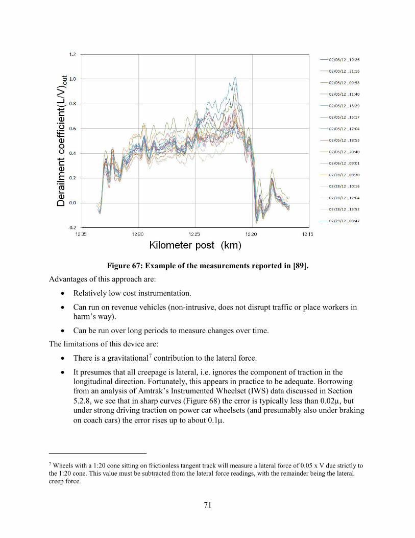
71
Figure 67: Example of the measurements reported in [89].
Advantages of this approach are:
• Relatively low cost instrumentation.
• Can run on revenue vehicles (non-intrusive, does not disrupt traffic or place workers in harm’s way).
• Can be run over long periods to measure changes over time. The limitations of this device are:
• There is a gravitational7 contribution to the lateral force.
• It presumes that all creepage is lateral, i.e. ignores the component of traction in the longitudinal direction. Fortunately, this appears in practice to be adequate. Borrowing from an analysis of Amtrak’s Instrumented Wheelset (IWS) data discussed in Section 5.2.8, we see that in sharp curves (Figure 68) the error is typically less than 0.02µ, but under strong driving traction on power car wheelsets (and presumably also under braking on coach cars) the error rises up to about 0.1µ.
7 Wheels with a 1:20 cone sitting on frictionless tangent track will measure a lateral force of 0.05 x V due strictly to the 1:20 cone. This value must be subtracted from the lateral force readings, with the remainder being the lateral creep force.
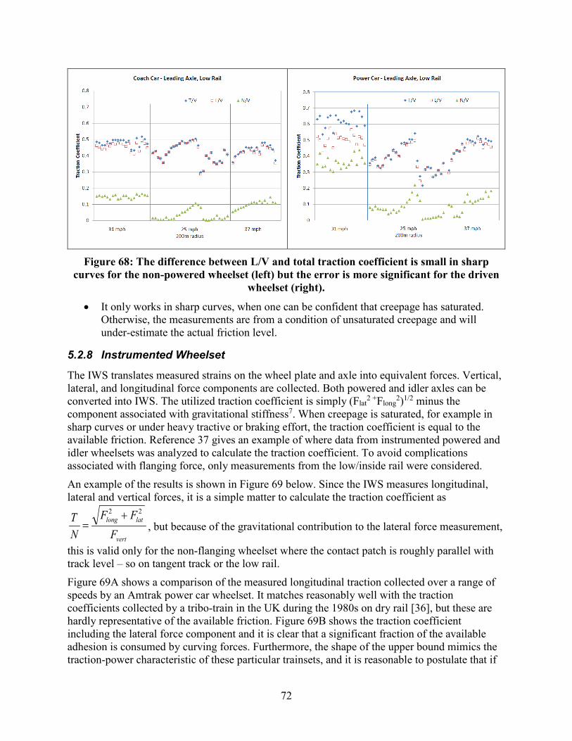
72
Figure 68: The difference between L/V and total traction coefficient is small in sharp curves for the non-powered wheelset (left) but the error is more significant for the driven
wheelset (right).
• It only works in sharp curves, when one can be confident that creepage has saturated. Otherwise, the measurements are from a condition of unsaturated creepage and will under-estimate the actual friction level.
5.2.8 Instrumented Wheelset
The IWS translates measured strains on the wheel plate and axle into equivalent forces. Vertical, lateral, and longitudinal force components are collected. Both powered and idler axles can be converted into IWS. The utilized traction coefficient is simply (Flat
2 +Flong2)1/2 minus the
component associated with gravitational stiffness7. When creepage is saturated, for example in sharp curves or under heavy tractive or braking effort, the traction coefficient is equal to the available friction. Reference 37 gives an example of where data from instrumented powered and idler wheelsets was analyzed to calculate the traction coefficient. To avoid complications associated with flanging force, only measurements from the low/inside rail were considered.
An example of the results is shown in Figure 69 below. Since the IWS measures longitudinal, lateral and vertical forces, it is a simple matter to calculate the traction coefficient as
vert
latlong
FFF
NT 22 +
= , but because of the gravitational contribution to the lateral force measurement,
this is valid only for the non-flanging wheelset where the contact patch is roughly parallel with track level – so on tangent track or the low rail.
Figure 69A shows a comparison of the measured longitudinal traction collected over a range of speeds by an Amtrak power car wheelset. It matches reasonably well with the traction coefficients collected by a tribo-train in the UK during the 1980s on dry rail [36], but these are hardly representative of the available friction. Figure 69B shows the traction coefficient including the lateral force component and it is clear that a significant fraction of the available adhesion is consumed by curving forces. Furthermore, the shape of the upper bound mimics the traction-power characteristic of these particular trainsets, and it is reasonable to postulate that if
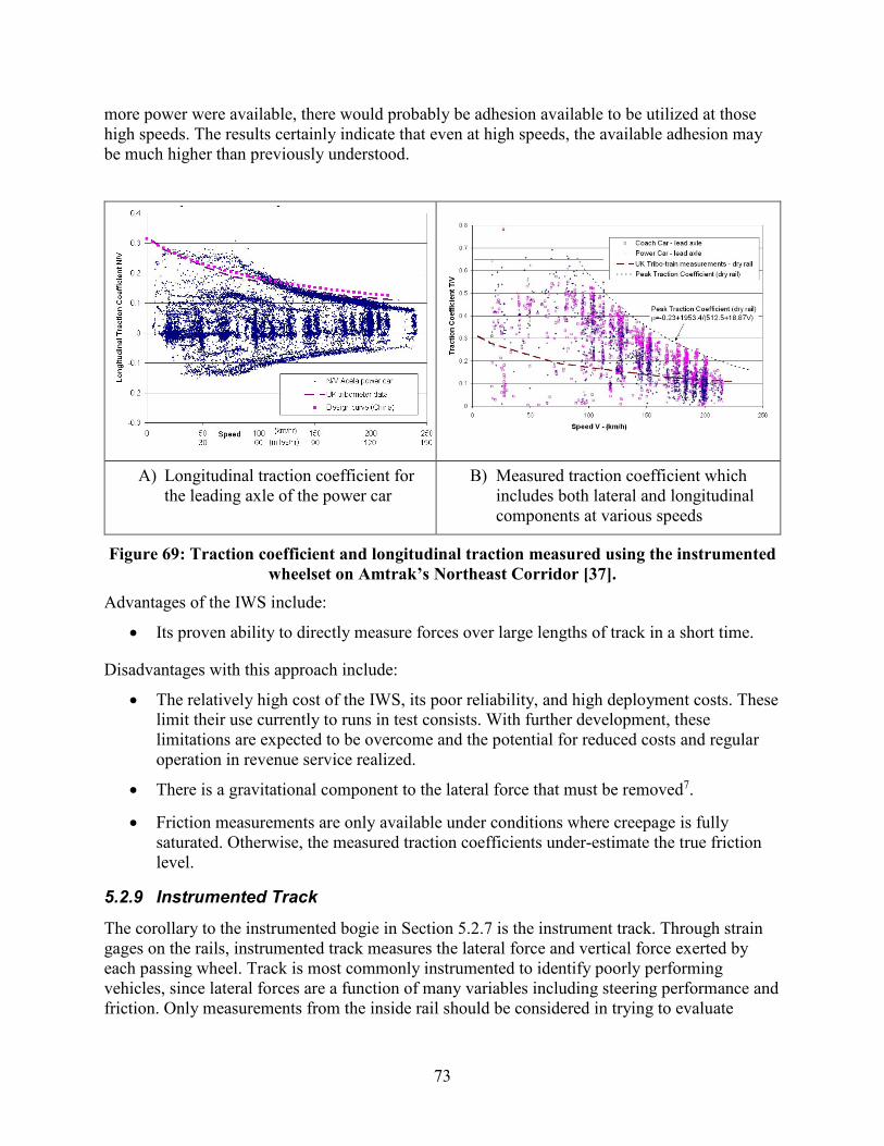
73
more power were available, there would probably be adhesion available to be utilized at those high speeds. The results certainly indicate that even at high speeds, the available adhesion may be much higher than previously understood.
A) Longitudinal traction coefficient for the leading axle of the power car
B) Measured traction coefficient which includes both lateral and longitudinal components at various speeds
Figure 69: Traction coefficient and longitudinal traction measured using the instrumented wheelset on Amtrak’s Northeast Corridor [37].
Advantages of the IWS include:
• Its proven ability to directly measure forces over large lengths of track in a short time.
Disadvantages with this approach include:
• The relatively high cost of the IWS, its poor reliability, and high deployment costs. These limit their use currently to runs in test consists. With further development, these limitations are expected to be overcome and the potential for reduced costs and regular operation in revenue service realized.
• There is a gravitational component to the lateral force that must be removed7.
• Friction measurements are only available under conditions where creepage is fully saturated. Otherwise, the measured traction coefficients under-estimate the true friction level.
5.2.9 Instrumented Track
The corollary to the instrumented bogie in Section 5.2.7 is the instrument track. Through strain gages on the rails, instrumented track measures the lateral force and vertical force exerted by each passing wheel. Track is most commonly instrumented to identify poorly performing vehicles, since lateral forces are a function of many variables including steering performance and friction. Only measurements from the inside rail should be considered in trying to evaluate
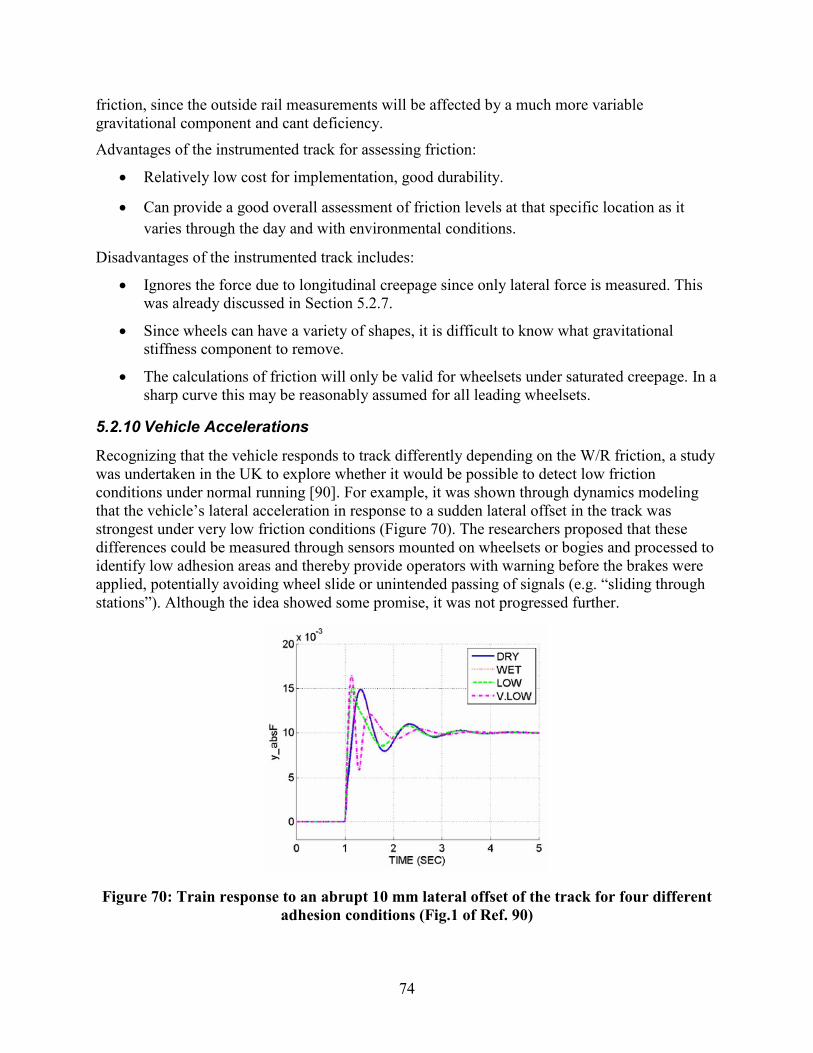
74
friction, since the outside rail measurements will be affected by a much more variable gravitational component and cant deficiency.
Advantages of the instrumented track for assessing friction:
• Relatively low cost for implementation, good durability.
• Can provide a good overall assessment of friction levels at that specific location as it varies through the day and with environmental conditions.
Disadvantages of the instrumented track includes:
• Ignores the force due to longitudinal creepage since only lateral force is measured. This was already discussed in Section 5.2.7.
• Since wheels can have a variety of shapes, it is difficult to know what gravitational stiffness component to remove.
• The calculations of friction will only be valid for wheelsets under saturated creepage. In a sharp curve this may be reasonably assumed for all leading wheelsets.
5.2.10 Vehicle Accelerations
Recognizing that the vehicle responds to track differently depending on the W/R friction, a study was undertaken in the UK to explore whether it would be possible to detect low friction conditions under normal running [90]. For example, it was shown through dynamics modeling that the vehicle’s lateral acceleration in response to a sudden lateral offset in the track was strongest under very low friction conditions (Figure 70). The researchers proposed that these differences could be measured through sensors mounted on wheelsets or bogies and processed to identify low adhesion areas and thereby provide operators with warning before the brakes were applied, potentially avoiding wheel slide or unintended passing of signals (e.g. “sliding through stations”). Although the idea showed some promise, it was not progressed further.
Figure 70: Train response to an abrupt 10 mm lateral offset of the track for four different adhesion conditions (Fig.1 of Ref. 90)
75
6. Conclusion
This survey of railway friction problems has identified a number of gaps in knowledge, expertise, and processes. They are summarized in the subsections that follow.
6.1 Instrumentation
Since friction is highly dependent upon the local conditions of rail and wheel, regular measurement is the only way to determine what values prevail at a given location on a railroad; while the standard Salient push-tribometer is very capable of providing a reasonable indication of friction level, it is unable to provide the fuller characterization needed in today’s sophisticated multi-body dynamics programs. At its simplest level, there are two properties required—the peak friction level and the saturation creepage. A more detailed analysis would include the full traction-creepage relationship.
Presently, there are four approaches to characterize friction:
1. Perform small-scale laboratory tests with systems able to closely control creepage and to measure the effective traction coefficient. The interfacial contaminants can be either naturally occurring as a result of wear and humidity, or deliberately introduced for characterization, such as abrasives and friction modifiers.
2. Perform full-scale laboratory simulations where the natural wear processes and composition of the interfacial layer are likely to be more representative of the field scenario. Like the smaller scale rigs, it is usually possible to control the W/R creepage and measure the required forces for calculating the traction coefficient.
3. Utilize special instrumentation on locomotives that allows ready access to the operating traction and creepage conditions.
4. Develop field instruments capable of measuring the traction-creepage relationship. At the time of this report, there were three instruments theoretically capable of doing this, but none had seen significant use. It is anticipated the new instrument from International Engineering will meet the need and with wider use, facilitate the development of a friction library for use by dynamic simulation packages for modeling derailment, wear and RCF.
The characteristics of the interfacial layer are poorly known. Because of the difficulty in getting on revenue track for long lengths of time, the use of x-ray diffraction, Glow Discharge-Optical Emission Spectroscopy, and other tools is not practical at the moment. A field instrument able to quickly characterize the composition of the interfacial layers is needed. Ideally, the instrument would be portable (could be carried by one person), self-contained (e.g., include its own power), and able to collect a spot measurement in 5 minutes or less, compared with the 30-50 minutes currently required.
6.2 Gage-face/Wheel-flange
Gage-face/wheel-flange contact can be particularly severe with very high contact stresses as well as large creepage. While the concept of lubricating that region is over a hundred years old, there is still considerable opportunity to improve applicator technology, fine-tune dispensing rates, and advance the lubricant formulations. First, answers to the following questions are required:
76
• What are the friction levels in the dry wheel flange contact?
• Under what conditions, presumably related to mechanical, chemical and surface energy considerations, are lubricants most effectively transferred from the wayside gage face distribution unit to the wheel flange?
• What is the relationship between grease composition and retentivity?
• Is there an effective test to determine the lower temperature limit at which lubricant can be picked up by the wheel flange?
• Is there an effective test to assess “carry down” at higher temperatures?
6.3 Modeling
It is well understood that the use of a Coulomb friction condition and the Kalker relationship is inadequate in simulating real-world phenomenon. While one approach is to scale the Kalker relationship (see Section 3.2), it does not account for the negative friction characteristic (see Section 2.4.1) that is at the root of important W/R phenomenon, including corrugation, wheel squeal, and the requirement for electronic adhesion and braking control systems. An improved relationship is needed and this needs to be accessible to multi-body dynamics simulations. Key questions to consider would be:
• How many and which parameters are required to adequately define the creepage-creep force relationship?
• What effect do these parameters have on typical W/R contact and vehicle dynamics behaviour?
• And if using the %KALKER approach, is there a logical and consistent method for choosing the scaling factor?
6.4 Testing
While it is possible in the laboratory to demonstrate the practical impacts of friction modifiers on the rates of wear and rolling contact fatigue, convincing field evidence has been difficult to obtain thus far. Well-controlled field tests are still needed.
Laboratory and field measurements of the traction-creepage relationship for a range of practical conditions, including high speeds, are needed both to improve understanding and for use in calibrating friction models. These tests need to include realistic interfacial layers.
There is little understanding of the friction characteristic at very low temperatures. Although low temperature performance would be important only for the first few rolling cycles until the surface warmed up, it is relevant for train startup in cold weather or perhaps for a crane operating in winter conditions.
6.5 Products
For adhesion enhancement, sand is commonly used. Since sand contributes to ballast fouling, is heavy in weight, and can freeze and clump in the reservoir, better adhesion enhancement agents are needed. They must be compatible with existing dispensing systems. The high cost of

77
alternative options will need to be taken into consideration as it could prove to be a challenge to overcome.
78
7. References
1. Lewis R. & Olofsson U. (2009). Wheel–rail interface handbook, Cambridge, UK, Woodhead Publishing Limited.
2. Rowell, B. & Richardson, W.S. (June 2003). An assessment of the available adhesion and slip risk for ERTMS, report # AEATR-VTI-2003-019, Issue 1 produced for the UK Rail Safety and Standards Board.
3. Sroba, P., Magel E., Caldwell, R. (2005). Testing of rail friction management on the 377.2 Baltimore Curve, NRC Report #54-A62209-T11-2-AUG05.
4. Halling J. (ed). (1978). Principles of Tribology, Great Britain, MacMillan Education Ltd.
5. Bowden, F.P. and Tabor, D. (1954). The friction and lubrication of solids, Oxford, Clarendon Press.
6. Tabor. D. (1951). The Hardness of Metals, Oxford, Clarendon Press.
7. Tabor, D. (1959). Junction growth in metallic friction: the role of combined stresses and surface contamination, Proceedings of the Royal Society of London, Series A, Mathematical and Physical Sciences, vol. 251.
8. Nadai, A. (1931). Plasticity, New York, McGraw Hill.
9. Bowden F.P. & Tabor, D. (1964). The friction and lubrication of solids, Pt. II, Oxford University Press.
10. Broster, M., Pritchard, C. & Smith, D.A. (1974). Wheel/rail adhesion: its relation to rail contamination on British Railways, Wear, Vol. 29.
11. Niccolini, E. & Berthier, Y. (2005). Wheel–rail adhesion: laboratory study of “natural” thirdbody role on locomotives wheels and rails, Wear, Vol. 258.
12. Suzumura J. et al. (2011). In situ X-ray analytical study on the alteration process of iron oxide layers at the railhead surface while under railway traffic, Wear, Vol. 271.
13. Beagley, T.M. (1976). Severe wear of rolling sliding contacts, Wear, Vol. 36.
14. Arias-Cuevas, O. et al. (2010), Rolling-sliding laboratory tests of friction modifiers in dry and wet wheel-rail contacts, Wear, Vol. 268.
15. Olofsson, U. & Sundvall, K. (2004). Influence of leaf, humidity and applied lubrication on friction in the wheel-rail contact pin-on-disc experiments, Proceedings of the IMechE Part F, Journal of Rail and Rapid Transit, Vol. 218, pp. 235–242.
16. Rowe, G. (2004). Metronet Rail Group, Central Line Leaf Fall Management, presentation.
17. Zhu, Y. (December 2011). Adhesion in the wheel/rail contact under contaminated conditions, Licentiate thesis, Royal Institute of Technology, Stockholm, Sweden.
18. Kalker, J.J. (1967). On the rolling contact of two elastic bodies in the presence of dry friction, Doctoral Dissertation, Technical University Delft, Delft, Netherlands.
19. Hobbs, A.E.W. (1967). A survey of creep. British Rail Dpt. DYN 52, Derby, UK.
79
20. Harrison, H., McCanney, T. & Cotter, J. (2003), Recent developments in coefficient of friction measurements at the wheel/rail interface, Wear Vol. 253.
21. Logston, C.F. & Itami, G.S. (1980)., Locomotive Friction-Creep Studies, ASME Journal of Engineering for Industry, Vol. 102, pp. 275–281.
22. Polach, O. (2006). Comparability of the non-linear and linearized stability assessment during railway vehicle design, Vehicle System dynamics: International Journal of Vehicle Mechanics and Mobility, Vol. 44.
23. Vollebregt, E.A.H. (2014). Numerical modeling of measured railway creep versus creep-force curves with CONTACT, Wear, Vol. 314, pp. 87–95.
24. Persson, B.N.J. (2000). Sliding Friction: Physical Principles and Applications, New York: Springer Verlag.
25. Hou, K., Kalousek, J. & Magel, E. (1997). Rheological model of solid layer in rolling contact, Wear, Vol. 211, pp. 134–140.
26. Meierhofer, A. et al. (2014). Third body Layer – experimental results and a model describing its influence on the traction coefficient, Wear, Vol. 314.
27. Wu H., Shu X. and Wilson N. (2005). Flange Climb Derailment Criteria and Wheel/Rail Profile Management and Maintenance Guidelines for Transit Operations, TCRP Report 71, Vol. 5, Washington, DC.
28. Ban, T. et al. (2004). A study on the coefficient of friction between rail gauge corner and wheel flange focussing on wheel machining, Proceedings International Wheelset Congress, Orlando, FL.
29. Zhu, Y. & Oloffsun. U. (2012). An Adhesion Model for Wheel–Rail Contact at the Micro Level Using Measured 3D Surface, Proceedings of 9th International Conference on Contact Mechanics and Wear of Rail/Wheel Systems, Chengdu, China, pp. 26.1.
30. Lundmark, J., Hoglund, E. & Prakesh, B. (2006). Running in behavior of rail and wheel contacting surfaces, Proceedings, International Conference on Tribology, Italy.
31. Grassie, S. (April 1997). Requirements for transverse railhead profile and railhead roughness following grinding, 6th International Heavy Haul Conference, Cape Town, South Africa.
32. Magel, E. & Kalousek, J. (2002). The application of contact mechanics to wheel rail profiles and rail grinding, Wear Vol. 253, pp 308–316.
33. Popovici, R. (February 2010). Friction in Wheel-rail contacts, PhD thesis, University of Twente, Enschede, The Netherlands.
34. Ohyama, T. (November 1991). Adhesion Characteristics of wheel/rail system and its control at high speeds, 4th RTRI Symposium, Tokyo, Japan.
35. Zhang, W. et al. (2002). Wheel/rail adhesion and analysis by using full scale roller rig, Wear, Vol. 253, pp. 82-88.
36. ORE Report 2, Question B164. (1990). Adhesion during Braking, and Anti-Skid Devices, Utrecht, Netherlands.
80
37. Magel, E.E. et al (2008), Traction, forces, wheel climb and damage in high speed railway operations, Wear, Vol. 265.
38. Tanvir. M.A. (1980). Temperature Rise Due to Slip Between Wheel and Rail- an Analytical Solution for Hertzian Contact, Wear, Vol. 61, No. 2, pp. 295–308.
39. Saka, N., Eleiche, A.M. & Suh N.P. (1997). Wear of metals at high sliding speeds, Wear, Vol. 44, pp. 109–125.
40. Polach, O. (2005). Creep forces in simulation of traction vehicles running on adhesion limit, Wear, Vol. 258.
41. Harrison, H. (2008). The development of a low creep regime, hand operated tribometer, Wear, Vol. 265.
42. Baek, K-S, Koygoku, K. & Nakahara, T. (2008). An experimental study of transient traction characteristics between rail and wheel under low slip and low speed conditions, Wear, Vol. 265.
43. Lewis, R. et al.. (2011). An alternative method for the assessment of railhead traction, Wear, Vol. 271.
44. Beagley, T.M., McEwan, I.J. & Pritchard, C. (1975). Wheel/rail adhesion – influence of railhead debris, Wear, Vol. 33.
45. Beagley, T.M. & Pritchard, C. (1975), Wheel-rail adhesion - the overriding influence of water, Wear, Vol. 35.
46. Cummings, S. & Kudinov, R. (August 2012). Seasonality of wheelset removals: Analysis of wheel and rail friction, AAR Technology Digest TD-12-016.
47. Oldknow, K., Eadie, D. & Stock, R. (January 2013). The influence of precipitation and friction control agents on forces at the wheel/rail interface in heavy haul railways, Proceedings of the Institution of Mechanical Engineers, Part F: Journal of Rail and Rapid Transit, Vol. 227, No. 1, pp. 86–93.
48. Ertz, M. & Bucher, F. (2003). Improved creep force model for wheel/rail contact considering roughness and temperature, Vehicle System Dynamics Vol. 37, pp. 314–325.
49. Pearce, T.G. & Rose, K.A. (1982). Tangential force – creepage relationships in theory and practice, Proceedings - Contact Mechanics and Wear of Rail/Wheel Systems, Vancouver, Canada.
50. Burstow, M.C. (September 2004). Whole life rail model application and development for RSSB, continued development of an RCF damage parameter, Report #AEAT-RES-2004-880.
51. Magel, E. & Liu, Y. (2009). Study of friction – measurement, analysis and practical implications for the wheel/rail contact, Proceedings - Contact Mechanics and Wear of Rail/Wheel Systems, Firenze, Italy.
52. Watkins, D.J. (1975). Exploring adhesion with British Rail’s tribometer train, Railway Engineering Journal, Vol. 4, No. 4.
53. VanderMarel, J. et al. (2012). A Predictive Model of Energy Savings from Top of Rail Friction Control, Proceedings of 9th International Conference on Contact Mechanics and Wear of Rail/Wheel Systems, Chengdu, China.
81
54. Suda, Y. et al. (2005). Development of onboard friction control, Wear, Vol. 258.
55. Fries, R. et al. (2011). Modeling of Friction Modifier and Lubricant Characteristics for Rail Vehicle Simulations, Proceedings IAVSD Symposium, Manchester, UK.
56. Fletcher, D.A. (2012). A new two-dimensional model of rolling–sliding contact creep curves for a range of lubrication types, Proc IMechE Part J: J Engineering Tribology Vol. 227(6) 529–537.
57. Vollebregt, E.A.H. (2014). Numerical modeling of measured railway creep versus creep-force curves with CONTACT, Wear, Vol. 314.
58. Tomberger, C. et al. (2011). Friction in wheel–rail contact: A model comprising interfacial fluids, surface roughness and temperature, Wear, Vol. 271.
59. Roney, M. et al. (2005). Canadian Pacific Railway’s 100% effective friction management strategy, Proceedings International Heavy Haul Conference, Rio de Janeiro, Brazil.
60. Eadie, D.T. et al. (2008). The effects of top of rail friction modifier on wear and rolling contact fatigue: Full scale rail-wheel test rig evaluation, analysis and modeling, Wear, Vol. 265, pp 122–1230.
61. Sroba, P. et al. (September 2001). Canadian Pacific Railway’s 100% effective lubrication initiative, Proceedings AREMA Annual Conference, Chicago, IL.
62. DeKoker, J. (October 1993). Rail and Wheel Flange Lubrication, South African Permanent Way Institute.
63. Magel, E. & Liu, Y. (2014). On some aspects of the wheel-rail interaction, Wear, Vol. 314.
64. Kalousek, J. (October 1976). Wear and Contact Fatigue Model for Railway Rail, NRC Technical Report, TR-WE-50, NRC No. 27491, TDC No. TP8344E.
65. Lewis, S.R. et al. (2014). “Assessment of railway curve lubricant performance using a twin-disc tester,” Wear, Vol. 314.
66. Aldajah, S.et al. (January 2005). Laser glazing of rails WBB-IWS tests (CNRC-Ottawa), ANL-05/03, Argonne National Laboratory.
67. Eadie, D. (January 2004). Experience with friction modifiers for noise and vibration reduction on North American transit systems, presentation: Transportation Research Board Annual Conference.
68. Matsumoto, A. et al. (2005). Improvement of bogie curving performance by using friction modifier to rail/wheel interface verification by full-scale rolling stand test, Wear, Vol. 258.
69. Cotter, J. et al. (2005). Top-of-Rail Friction Control: Reductions in Fuel and Greenhouse Gas Emissions, Proceedings International Heavy Haul Association Conference, Rio de Janeiro, Brazil.
70. Egana, J.I., Vinolas, J. & Gil-Negrete, N. (August 2005). Effect of liquid high positive friction (HPF) modifier on wheel-rail contact and rail corrugation, Tribology International, Vol. 38, Issue 8.
71. Eadie, D.T. et al. (2008). Field studies of the effect of friction modifiers on short pitch corrugation generation in curves, Wear, Vol. 265.
82
72. Eadie, D.T. et al. (2003). Top of Rail Friction Control: Lateral Force and Rail Wear Reduction in a Freight Application, Proceedings International Heavy Haul Association Specialist Technical Session, Dallas TX.
73. Li, Z. et al. (2009). Rolling–Sliding Laboratory Tests of Friction Modifiers in Leaf Contaminated Wheel–Rail Contacts, Tribology Letters, Vol. 33, pp. 97–109.
74. Ban, T. (June 2007). Friction Moderating System to Reduce Wheel/rail Interface Problems at Sharp Curves, Railway Technology Avalanche, No. 18.
75. Ishida, M., Ban, T. & Ogata, M. (June 2007). Friction Moderating System for Wheel/rail Interface to Reduce Lateral Forces in Sharp Curves, Proceedings International Heavy Haul Association Conference, Kiruna, Sweden.
76. Ohno, K., Ban, T. & Obara, T. (1996). Improvement of Adhesion Between Wheel and Rail by Ceramics Particle Injection, Journal of Japanese Society of Tribologists, Vol. 41, No. 12, pp.124–129.
77. Cotter, J. et al. (June 2005). Freight car-based top of rail friction modifier application system, Proceedings International Heavy Haul Association conference, Rio de Janeiro, Brazil.
78. Kelsan Technologies. (2004). Use of Top-of-Rail Friction Modifiers to Reduce Greenhouse Gas, TP#14851E Transport Canada Freight Transportation Case Studies.
79. Clayton P. & Hill, D.N. (1987). Rolling contact fatigue of a rail steel, Wear, Vol. 117.
80. Beynon, J.H., Garnham, J.E. & Sawley, K.J. (1996). Rolling contact fatigue of three pearlitic rail steels, Wear, Vol. 192.
81. Ishida, M., Ban, T. & Moto, T. (1998). The development of two-disc rolling contact test machine and some experimental results of checking its performance, Japan Rail Technology Joint Symposium, pp. 301–302 (in Japanese).
82. Matsumoto, A. et al. (1996). Wheel-rail contact mechanics at full scale on the test stand, Wear, Vol. 191.
83. WIDEM project newsletter No. 1. (2006). Available at http://www.widem.org/news.php.
84. Bogacz, R. & Konowrocki, R. (October 2012). On new effects of wheel-rail interaction, Archive of Applied Mechanics, Vol. 82, Issue 10-11, pp. 1313–1323.
85. BS 7976-1 (2002). Pendulum testers: part 1 – specification.
86. Surveyor High Speed Rail Tribometer, October 2015. Available at http://www.lbfoster-railtechnologies.com/pdf/brochures/PortecTRIBOMETER.pdf.
87. Matsumoto A. et al. (August 2012). Actual States of Wheel/Rail contact forces and friction on Sharp Curves, Proceedings 9th International Conference on Contact Mechanics and Wear of Rail/Wheel Systems, Chengdu China.
88. RSSB Research Brief. (December 2009). Investigating a novel method for estimating low adhesion conditions, Report T614.
83
Abbreviations and Acronyms
3BL Third Body Layer
DMF Diversified Metal Fabricators
EP Extreme Pressure
FM Friction Modified
FRA Federal Railroad Administration
GPS Global Positioning System
IWS Instrumented Wheelset
L/V Ratio of Lateral to Vertical Force
NRC National Research Council Canada
NRC-AST National Research Council Canada – Automotive and Surface Transportation
RCF Rolling Contact Fatigue
TOR Top of Rail
W/R Wheel/Rail
MoS2 Molybdenum Disulfide
Ra Average Surface Roughness
84
Definitions and Terminology
Adhesion: see Traction Coefficient
Creepage: non-dimensionalized slip, most commonly the difference in velocity of the two bodies divided by the average, i.e.
(v1-v2)/(0.5*(v1+v2))
Creep Saturation: see “Saturated Creepage.”
Dispatchable Adhesion: the minimum traction force a locomotive can develop under adverse conditions.
Friction (force): the shear force that resists relative motion between two surfaces in contact.
Friction Coefficient: the peak value of shear force/normal force that can be applied at the W/R contact before full slip.
Interfacial Layer: the thin film that normally exists at the W/R contact, separating the two surfaces and having a profound effect on friction.
Saturated Creepage: the value of creepage at which all points within the contact patch are in slip and beyond which the shear or traction force does not increase further.
Slip: a difference in the velocity of the wheel and rail surfaces that arises because of a yaw angle, traction or braking of the wheelset.
Traction-Creep Characteristic: the relationship illustrating how traction varies with creepage. See Section 2.4.
Traction Coefficient: the value of shear (or tractive) force divided by the normal force. At its limit, this is equal to the friction coefficient:
_/ FrictionNTAdhesion FF µµ ≤=
where FT is the tangential force and FN the force normal to the plane of the contact patch. Note that in the general case, FT has both longitudinal and lateral components.
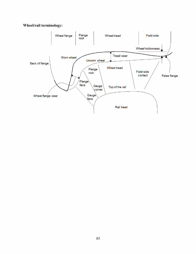
85
Wheel/rail terminology: