A Survey on Picture-Walking Automata

Jarkko Kari and Ville Salo

University of Turku

Abstract. Picture walking automata were introduced by M. Blum andC. Hewitt in 1967 as a generalization of one-dimensional two-way fi-nite automata to recognize pictures, or two-dimensional words. Severalvariants have been investigated since then, including deterministic, non-deterministic and alternating transition rules; four-, three- and two-waymovements; single- and multi-headed variants; automata that must stayinside the input picture, or that may move outside. We survey resultsthat compare the recognition power of different variants, consider theirbasic closure properties and study decidability questions.

Key words: Picture-walking automata, 2-dimensional automata, picturelanguages

1 Introduction

Informally, a picture is a matrix over a finite alphabet, and a picture languageis a set of matrices over the same alphabet. A picture-walking automaton is afinite state automaton moving on the cells of the given picture according to alocal rule, accepting if it reaches a final state [1].

The theory of picture languages is a branch of formal language theory whichstudies natural picture language families and connections between them. Mostof this theory has concentrated on classes having to do with ‘finite state’, in aneffort to find a natural counterpart for the one-dimensional regular languages.The classes obtained from picture-walking automata are usually not consideredto be a very natural counterpart due to their rather weak closure properties,but the recognizable picture languages take this place instead. In fact, manyinteresting proofs about picture-walking automata have more of a ‘navigational’than a language-theoretic feel to them.

In the first section, we deal with very basic and natural questions. We onlyconsider Boolean closure properties and the lattice of inclusions between thefour basic automata classes we define: DFA, NFA, UFA and AFA, that is, deter-ministic, non-deterministic, universally quantifying and alternating finite stateautomata, respectively. We present a slightly more refined view to these questionsby considering unary rectangles and non-unary square pictures separately withthe aim of clarifying the strengths and weaknesses of each approach. In each casewe obtain a slightly different set of non-closure properties, which taken togethergive a rather complete set of results for the class of all pictures.

The second section introduces a very modest-looking change to the definitionof an automaton: allowing it to exit the picture. We will see that this change isrelevant for AFA, but not for the other classes, although this is not altogetherstraightforward to prove. In the third and fourth sections, we introduce muchgreater changes to the definition. In the third section, we restrict the directionsin which the automaton is allowed to move. We give a brief introduction to theresults known for these classes. In particular, for three-way automata, we givea complete set of Boolean closure properties and complete comparison resultsbetween all three- and four-way automata classes, mostly without proofs. In thefourth section we give our automata a finite set of markers they can move aroundthe picture. In Section 5, we review decidability results, and recall connectionsbetween 2-dimensional DFA and Minsky machines.

Finally, we mention that a survey on two-dimensional picture-walking au-tomata theory already exists [2], although it’s main focus is not on finite stateautomata but on general Turing machines. Since few papers on picture-walkingautomata have been published after [2], it is still mostly up-to-date, except forsome open problems which have since been solved (many of which are presentedhere). There is also a good survey of general two-dimensional language theoryin the Handbook of Formal Languages [3].

2 Definitions

A picture is the two-dimensional analog of a finite word: a not necessarily squarematrix over a finite alphabet. We may usually assume a binary alphabet Σ ={0, 1}. We write Σ∗∗ for the full language of all matrices over Σ, and define apicture language as a subset of a full language. A class of picture languages,usually called a picture class, is a collection of picture languages.

For p ∈ Σ∗∗ we write p[(i, j)] = pi,j for the contents of the cell in position (i, j)in p, with the usual matrix indexing. We also draw p as a matrix, and thus, forinstance, the cell with index (1, 1) is considered the top left cell and the firstaxis is the vertical one, ascending downward. If (i, j) is not a cell of p, we definep[(i, j)] to be a special symbol # (that is, in practise we index pictures by Z2). Wewrite dom(p) for the set of indexes of (non-#) cells in p, called the domain of p,and edom(p) for the cells of dom(p) and all their neighbors. The width and heightof a picture p are denoted by |p| and p, respectively. The set edom(p)− dom(p)is called the border of p.

Let us start by defining the main picture-walking automata considered inthis survey, and their corresponding picture classes. Our automata have a singlehead, and they walk on the positions of the picture according to a local rule,accepting if they reach a final state. Existential and universal states can be usedto make (perfect) guesses and to check multiple local properties ‘simultaneously’,respectively.

Definition 1. An alternating finite state automaton (an AFA) A is a tuple(Q,Σ,E,U, I, F, δ) where Q is the set of states partitioned into E and U , the

sets of universal and existential states. The sets I, F ⊂ Q are called the sets ofinitial and final states. The function δ is called the transition function or thelocal rule and it has type δ : Q×Σ → 2Q×{(1,0),(−1,0),(0,1),(0,−1)}.

If Q = E (and thus U = ∅), the automaton is said to be non-deterministic(an NFA), and if Q = U and |I| = 1, it is said to be universally quantifying (aUFA). If all images of δ are singletons or empty sets and |I| = 1, the automatonis called deterministic (a DFA). We use the variable XFA to state things for allthe automata classes simultaneously.

Definition 2. Let A = (Q,Σ,E,U, I, F, δ) be an AFA. An instantaneous de-scription (an ID) of A on a picture p ∈ Σ∗∗ is a pair (q, x) ∈ Q × edom(p).An ID l2 = (q2, x2) is a successor of another ID l1 = (q1, x1) if (q2, x2 − x1) ∈δ(q1, p[x1]). We then write l1 → l2. For a vertex-labeled tree r, we write a1 → a2

if a2 is a child of a1 in r, and we write l(a) for the label of node a ∈ r.Now, an accepting run of A on p is a finite tree r labeled with ID’s such that

– the root of r has its label in I × {(1, 1)}.– if a1 ∈ r is not a leaf and l(a1) ∈ E × edom(p), then

∃a2 ∈ r : a1 → a2 ∧ l(a1)→ l(a2).

– if a1 ∈ r is not a leaf and l1 = l(a1) ∈ U × edom(p), then

∀l2 : l1 → l2 =⇒ ∃a2 ∈ r : a1 → a2 ∧ l(a2) = l2.

– the leaves of r have labels in F × edom(p).

We write L(A) for the set of pictures p over Σ for which there exists anaccepting run of A.

The restriction |I| = 1 is important for UFA, since otherwise I provides theautomaton with existential quantification. For DFA, NFA and UFA, we mayleave E and U out of the definition, and for DFA, we take δ to have the typeδ : Q×Σ → Q× {(1, 0), (−1, 0), (0, 1), (0,−1)}, with the obvious meaning.

Note that an accepting run for an NFA is just a sequence of ID’s. For UFA,an accepting run can look complicated, but we may – in an obvious way – definenon-accepting runs for them, that is, possibly infinite sequences of ID’s that proveno accepting run exists. This is possible since all choices of transitions must leadto acceptance or a picture is rejected by a UFA. Of course, a non-accepting runexists if and only if the picture is not accepted.

Note that our automata cannot sense if the border of the picture is next tothem, but must step on it and read the special symbol # in order to obtainthis information. We will also need 1-dimensional automata. These are alwaystwo-way automata, that is, they move both left and right. The left and rightends of the input word are again observed by reading a bordering #.

For each automata class XFA, the picture class corresponding to XFA willalso be called XFA. That is, asking whether there exists an XFA for a picture

language L is equivalent to asking whether L ∈ XFA. This should not causeconfusion.

We use the naming scheme of [4] and [5] for the XFA classes. DFA andNFA were defined already in [1] in 1967 and were simply called ‘automata’,while the most used names for DFA and NFA seem to have been ‘2-DA’ and‘2-NA’, respectively. UFA and AFA were discussed at least in [6], as a subset ofTuring machines, and were given the names ‘2-UFA’ and ‘2-AFA’ in [7]. Slightlyconfusingly, we will later write 2XFA to refer to two-way automata instead oftwo-dimensional automata. Two- and three-way restrictions of automata haveoften been denoted by having ‘TR’ and ‘TW’ somewhere in the name of the class,respectively. We do not consider probabilistic automata in this article: see [8] fora incomparability result between probabilistic automata and AFA.

The square pictures and the unary pictures are natural subclasses of the setof all pictures (also called the general pictures). Some negative results (results ofthe type L /∈ CLS for some picture class CLS) are easier to prove in the squareworld (content results) and some are easier to prove in the unary world (shaperesults).

Definition 3. For each automata class XFA, we write XFAs for the languagesof square pictures accepted by some automaton in XFA. We write XFAu for theunary languages of the XFA automata. Complements of languages in XFAs andXFAu are usually taken with respect to the set of all square pictures and all unarypictures, respectively.

The theory of picture languages has not been primarily concerned with thesekinds of automata, but a different model of computation known as recogniz-ability. We will not discuss the recognizable picture languages (REC) in length,but we do show some connections between the two worlds, and obtain someresults for picture-walking automata from non-closure properties of REC. Formore information on REC, see [3] or [5].

Definition 4. A Wang tile is an element of C4 for some set of colors C con-taining a special element #. A set T of Wang tiles with the same C defines apicture language over T by taking the pictures where neighboring colors match,and #’s occur (only) facing the border of the picture. Such a language is calleda local picture language. A recognizable picture language is the image of a localpicture language through a symbol-to-symbol projection. We denote the class ofrecognizable picture languages by REC.

We may also think of an REC grammar (tileset and projection) as ‘accept-ing’ languages instead of generating them, by taking a picture p, and assigning‘states’ (elements of T ) on top of the cells of p, which agree in their colors withthe neighboring states. When picture-walking automata are involved, we will,however, avoid the term ‘state’ in this context, and simply say tiles are assignedon top of the cells.

3 Basic results on 4-way automata

As is often the case in mathematics, the main results in the theory of picture-walking automata tend to be of one of two types: ‘positive’ or ‘negative’. Apositive result says a class is a subset of another, or that a language belongs toa class, while a negative result tells us a class is a proper subset of another, orthat a language cannot be accepted by some type of machine.

Many negative results are known for both XFAu and XFAs, and taken to-gether, one could say the natural questions for XFA have mostly been answered.However, the intersection of these classes is not understood at all. We repeat thefollowing two conjectures, which were made in [9] in 2004, and are still unan-swered.

Conjecture 1. The language of unary squares with prime side length are not inDFA.

Conjecture 2. DFA is a proper subset of NFA when restricted to unary squares.

As we mentioned, by varying either shape or content, we can build the begin-ning of a (proper) polynomial hierarchy and prove basic non-closure propertiesfor all the automata classes involved. We first show positive results for the classof all picture languages and then devote a subsection for negative results in boththe case of varying shape with unary alphabet and varying content with squareshape. In the unary case, a proper diamond of inclusions is shown to exist be-tween the four classes. As for the square case, proper inclusions are known tohold between DFAs, NFAs and AFAs, but little is known about UFAs. In eachcase a slightly different set of Boolean closure properties is obtained.

Figure 1 summarizes the known results. All inclusions drawn are proper, anddashed lines signify incomparable classes. On the right side, UFAs is known tobe between DFAs and AFAs, but not between DFAs and NFAs.

Fig. 1. A diagram of inclusions of the automata classes in the unary and square case.

Picture languages

?

Unary

DFAu

NFAu UFAu

AFAu

Square

DFAs

NFAs UFAs

AFAs?

?

In the following sections, we will see that DFA is closed under complementa-tion, while NFA, UFA and AFA are not. We prove non-closure under complementseparately for the unary and square cases for NFA and UFA. Non-closure in thecase of all pictures can easily be inferred from either proof. The case of comple-menting AFAu is unknown, but we prove non-closure for AFAs, from which thegeneral case of AFA easily follows. Figure 2 summarizes the closure propertiesknown for the different types of automata, where we write XFAx for XFA, XFAu

and XFAs.

Fig. 2. Refined table of Boolean closure properties of the XFA classes.

DFAx NFA NFAu NFAs UFAx AFA AFAu AFAs

¬ Yes No No ? No No ? No

∩ Yes Yes Yes Yes Yes Yes Yes Yes

∪ Yes Yes Yes Yes ? Yes Yes Yes

Note that for general pictures, all Boolean closure properties except for theclosure of UFA under union are known. In [5], a negative answer is conjectured.

Conjecture 3. UFA is not closed under union.

3.1 Positive results

Obviously, DFA ⊂ NFA ⊂ AFA and DFA ⊂ UFA ⊂ AFA with not necessarilyproper inclusions. It is also clear that all the classes are closed under rotationaround the center of the picture, vertical and horizontal flips and matrix trans-pose. We can also prove natural Boolean closure properties for these classes withsimple constructions outlined below.

The following observation has been used in numerous articles, including [7,4, 5]. The proof is a direct modification of [10].

Theorem 1. For every DFA A, there is a DFA A′ with L(A′) = L(A) such thatA′ halts on every input.

Corollary 1. DFA is closed under complementation, that is, DFA = co-DFA.

Theorem 2. All the XFA classes are closed under intersection and DFA, NFAand AFA are closed under union.

Proof. Since an accepting computation is necessarily halting in all branches ofthe accepting run, intersection can be implemented for any machine by simplytesting inclusion in the languages in question one by one. As for union, NFAand AFA can use an existential state, and for a halting DFA (guaranteed byTheorem 1), union can be implemented like intersection.

3.2 Negative results for varying shape and unary alphabet

The shape-based approach is more recent than the content-based one, and givesbetter results for connections between classes. It is based on 1-dimensional au-tomata. The tools we need are a reduction from 2D to 1D (Lemma 1) and alemma connecting the number of states in a 1-dimensional automata, and theperiod and threshold of its language (Lemma 2). After this, a single concretelanguage is enough to separate all the four automata classes. We also obtainnon-closure under complementation for NFAu and UFAu.

Let A be an XFA running on unary input, with language L = L(A). Foreach height h, we may, in a natural way, associate a 1-dimensional XFA Ahaccepting the unary language of the corresponding widths. Furthermore, Ah hasO(h) states where the invisible constant only depends on A.

Lemma 1. [4] Let A be an AFA with ku universal states and ke existentialstates recognizing the unary picture language L ⊂ {1}∗∗. Then, for each h, thelanguage Lh = {1|p| | p ∈ L, p = h} is recognized by a one-dimensional two-wayAFA Ah with ku(h+ 2) universal states and ke(h+ 2) existential states.

Proof. Let A = (Q, {1}, E, U, I, F, δ) and X = [0, h+ 1]. Then

Ah = (Q×X, {1}, E ×X,U ×X, I × {1}, F ×X, δh)

where δh simulates the local rule of A, interpreting the location of Ah as thehorizontal location of A, and the X component of the state of Ah as the verticallocation of A. It is clear that Ah correctly recognizes Lh.

Of course, each Ah accepts a unary regular language, and thus an eventuallyperiodic language. Since the Ah have linearly many states with respect to h, itwill be useful to prove a lemma which tells us something about the connectionbetween the number of states in a (one-dimensional) automaton, and the periodand threshold of the unary language it accepts.

Lemma 2. [4, 5] Let A be a 1D (two-way) AFA with k states over a unaryalphabet with language L ⊂ 1∗. Let n > k. Then

– if A is an NFA, 1n ∈ L =⇒ 1n+k! ∈ L.– if A is a UFA, 1n ∈ L⇐= 1n+k! ∈ L.

In particular, if A is a DFA, an equivalence holds, since if the transitionrelation is a function, we may change between universal and existential stateswithout changing the language.

Proof. First, assume all states are existential, and let 1n ∈ L. Consider a subse-quence s of an accepting run r for 1n, which visits border symbols # at s1 ands|s| or possibly ends with the automaton halting in the middle of the word (wethink of the automaton as being on the left border just before starting its run).We will translate such ‘partial runs’ to corresponding partial runs for the longerinput 1n+k!, which we then glue together to obtain 1n+k! ∈ L.

If a partial run moves from the left border back to the left border, the samepartial run can be used for the longer input, and similarly for the right border.If a partial run ends in the middle of the word, it can also directly be translatedfor the longer word.

If s moves from the left border to the right border, we note that there mustbe a repetition of states such that the automaton moved some number of steps0 < l ≤ k to the right in between. But l divides k!, so we may repeat this partialrun an additional k!

l times to obtain a corresponding partial run for the longerinput. A similar claim holds for partial runs from right to left.

The claim for UFA follows by considering non-accepting runs instead. Thefact that these runs can be infinite does not lead to complications.

We will now separate NFA and UFA by using the duality between existentialand universal quantification found in Lemma 2. For this, we will use the following‘billiard ball language’ from [4].

Definition 5. The billiard ball language Lbilliard is defined as

Lbilliard = {p ∈ {1}∗∗ | |p| ∈ 〈p, p+ 1〉} = {mp+ n(p+ 1) | m,n ∈ (N ∪ 0)}

Fig. 3. The movement of an NFA accepting the unary 3x10 picture, which is in Lbilliard.

That is, for each height h, the widths must be some linear combination ofh and h + 1. It is easy to make an NFA accepting this language by having itmove to the right diagonally, bouncing off the walls as in Figure 3. Just as easily,we can make a UFA accepting its (unary) complement. Using the lemmas weproved, we can also prove the converse claims: a UFA cannot accept Lbilliard andan NFA cannot accept its complement:

Lemma 3. Lbilliard /∈ UFAu, Lcbilliard /∈ NFAu

Proof. We will only prove Lbilliard /∈ UFAu, the proof for NFAu is symmetric. Soassume on the contrary that A is a UFA with k states accepting Lbilliard, and foreach h let Ah with L(Ah) = Lh be the 1-dimensional UFA given by Lemma 1.

By looking at the definition of Lbilliard, it is not hard to see that for each h,h2−h− 1 = h(h− 2) + (h− 1) is not in Lh, but h2−h is. Let h be large enoughthat h2−h−1 > k(h+2). Here, k(h+2) = kh is the number of states of Ah, and1h

2−h−1 /∈ Lh, so by Lemma 2, also 1h2−h−1+mkh! /∈ Lh for all m. But obviously

Lh contains every word longer than some threshold t, a contradiction.

Corollary 2. NFAu ./ UFAu.

Corollary 3.DFAu ( NFAu ( AFAu

andDFAu ( UFAu ( AFAu

Thus, we have built the diamond on the left in Figure 1. As a side product,we obtained that NFA and UFA are not closed under complement, completingthe unary part of Figure 2.

Corollary 4. NFAu and UFAu are not closed under complement.

3.3 Negative results for varying content and square shape

The separation of DFA and NFA on binary squares was done already in [1], andit is based on a pigeonhole argument.

Definition 6. The language Lcenter consists of square pictures p of odd sidelength over {0, 1} containing a 1 in the middle cell.

Theorem 3. Lcenter is in NFAs −DFAs.

Proof. It is easy to see that Lcenter is in NFAs: An NFA for it follows the maindiagonal southeast, and can turn northeast at any 1 it sees. It accepts if it reachesthe northeast corner. (Checking that the picture has square shape is trivial.)

Now, consider a hypothetical DFA A = (Q,Σ, I, F, δ) for it. We may assumeA always leaves the domain of the picture before accepting it, and that it alwayshalts by Theorem 1. To each binary n × n picture p we can then associate afunction fp characterizing the behavior of A inside the picture p. The functionfp has the type

fp : Q× E(p)→ Q× (edom(p)− dom(p)),

where E(p) is the set of cells of p with a neighbor outside dom(p), and fp((q, x)) =(q′, x′) if from the ID (q, x), A eventually leaves the domain of p in ID (q′, x′)(this is well-defined by the assumptions we made).

For some constant C depending only on A, we have that for any n thereare less than Cn elements in Q× E(p), and there are less than Cn elements inQ× (edom(p)−dom(p)). Therefore, there are less than CnCn different functionsfp for a fixed side length n. Of course, there are 2n

2pictures p with side length

n.By taking n large enough that CnCn < 2n

2, we thus obtain two pictures of

side length n with p[x] 6= q[x] for some x, but fp = fq. Now we can construct twolarger pictures p′ and q′ that agree everywhere except at a subpicture where p′

has a translated copy of p and q′ has q such that the position x is moved to themiddle of the larger pictures. One of these pictures is in Lcenter and the other isnot, but A will obviously accept p′ if and only if it accepts q′, a contradiction.

By Theorem 1, we then have the following.

Corollary 5. DFAs ( NFAs.

The proofs involving universal states use non-closure properties of REC. Ofcourse, we will first need to prove some connections between the automata classesand REC. Theorem 5 and its natural corollaries first appeared in [7], and inde-pendently in [4] where also Theorem 4 and its natural corollaries were proven.We will only scetch these proofs, more details can be found in [7] and [5]. Theproofs are for general pictures.

Theorem 4. NFA ⊂ REC.

Proof. For an NFA, we construct a set of Wang tiles whose valid tilings drawaccepting runs of the NFA on top of the picture. This is done by carrying theset of states the NFA can reach at each tile. The top left corner must contain aninitial state, and some tile must contain a final state. The problem is we needto make sure a final state can only occur if there is a path to it from the topleft corner. To achieve this, every state contained in a tile (except the initialstate at the top left corner) will have a single predecessor, and a final state isthe predecessor of no state. Then no loops containing a final state can occur, soa chain of successor links ending in a final state must have started at the initialstate at the top left cell – and thus represents a valid loopless computation ofthe NFA.

Theorem 5. co-AFA ⊂ REC.

Proof. For this, we construct a set of Wang tiles whose valid tilings depict failedcomputations. Again, tiles contain a set of states, and a tile contains a state ifthere is no accepting computation from that state. The top left tile must containall the initial states, a universal state must have at least one successor in theneighboring tiles (at least one choice of action leads to a failing computation),and an existential state must have all its successors in neighboring tiles (everypossible choice of action leads to a failing computation). No final states mayoccur. It is then easy to believe that a tiling exists if and only if the automatondoesn’t accept the input picture.

Next, we will need a concrete language. Let Lacyclic be the language of (notnecessarily planar) acyclic graphs. Any representation of graphs where the graphsare somehow ‘drawn’ on the (square) picture will do. We will assume a node canbe contained in every cell, an edge can go through multiple cells, edges can crosseach other freely, and a large (but fixed) number of them can move through asingle cell.

We note that Lacyclic is in UFAs, since an automaton can use universal statesto check that every possible run along the forward edges of the graph leads toa dead end. However, a standard pigeonhole argument shows it is not in REC[4]: Split pictures of side length n in two, with a vertical border in the middle,containing n nodes. On both sides, implement the same total order, connecting

each node to its immediate successor. For large enough n, there are more partialorders than there are possible tilings of the middle column in tilings acceptingthe pictures representing the partial orders. Therefore, some two pictures canswap their right sides, necessarily resulting in a picture with a valid tiling, butwhich contains a cycle.

By the previous paragraph, UFAs cannot be a subset of NFAs, or it wouldalso be a subset of REC, which is contradicted by Lacyclic ∈ UFAs − REC. Wethus obtain the partial diamond on the right side in Figure 1.

Theorem 6.DFAs ( NFAs ( AFAs,

DFAs ( UFAs

andUFAs 6⊂ NFAs

Theorem 7. UFAs and AFAs are not closed under complement.

Proof. Otherwise,UFAs = co-UFAs ⊂ REC,

which is a contradiction. The case of AFAs is proved similarly.

Using the connection with REC, it is also easy to show certain non-closureproperties for all of the classes XFA simultaneously. We outline the idea for anoperation that inherently works on general pictures instead of squares: concate-nation. Consider the following lemma, which directly follows from Theorem 5.

Lemma 4. If f is an operation on languages, L1, . . . , Lk ∈ DFA but f(L1, . . . , Lk)c /∈REC, then none of the classes XFA are closed under the operation f .

This implies that we can prove certain non-closure properties working com-pletely within REC – and REC is very easy to work with!

Theorem 8. None of the classes XFA are closed under concatenation.

Proof. We prove the claim for horizontal concatenation. Consider the languageLl=r = {p ∈ Σ∗∗ | p[∗, 1] = p[∗, |p|]}, where Σ = {a, b, c}. Clearly, Ll=r is in DFA,and therefore in all of the classes. Consider the language L = Ll=rLl=rLl=r. Ifone of the classes XFA were closed under concatenation, then L would be in thisclass. We show that L is not even in the class AFA. If it were, then Lc wouldbe in co-AFA, and therefore also in REC by Theorem 5. We will show, however,that Lc is outside REC, proving the claim. Suppose, on the contrary, that Lc

were in REC.The language Lc is the the language of pictures p such that

∀i, j such that 3 ≤ i < j ≤ |p| − 2 :p[∗, i] = p[∗, j] =⇒ p[∗, 1] 6= p[∗, i− 1] ∨ p[∗, j + 1] 6= p[∗, |p|] ,

where p[∗, k] means the kth column of p. It looks kind of hard to work with,so we use the many well-known closure properties of REC to simplify it: Firstwe restrict to the subset of pictures with columns alternatingly over {c} and{a, b} and with additional borders over {c}. In other words, the rows will be inthe regular language given by the expression c(c(a + b))∗cc. This restriction isobtained by intersecting with a recognizable language. On this subset of Lc, theconstraint simply forbids equal columns over {a, b}. We then erase the columnsover {c} using further closure properties to obtain that the simpler language

Lc 6=c = {p | 6 ∃i 6= j : p[∗, i] = p[∗, j]}

is in REC. But it is proven in [5] that Lc 6=c is in fact not in REC, a contradiction.See [5] for the details.

4 Moving outside the picture

In this section, we think of pictures as being embedded on the plane Z2 in theposition indicated by the indexes. Thus, extending the indexing of matrices, theplane will be drawn with the first axis being the vertical one, and the second thehorizontal one, with the first coordinate increasing as we move down, and thesecond as we move to the right.

So far, we have considered automata that are not allowed to exit the picturethey are accepting. It is easy to see that a DFA does not gain any extra strengthif it is allowed to exit a picture [11]. The corresponding question of whether NFAare strengthened if they are allowed to exit the picture was solved for picturesof height 1 in [11] in the negative. The question remained open for arbitraryshapes [11, 12, 4], until a negative answer was given recently in [5]. The solutionis based on a theorem from [9] characterizing the languages of non-deterministicautomata that are not allowed to enter the picture they are accepting, and wewill outline the proof in Section 4.2. Also the case of AFA was solved in [5]. Inthis case, a simple example shows automata are in fact strengthened if they canexit the picture.

Definition 7. FNFA is the class of picture languages accepted by NFA that areallowed to exit the pictures they are accepting. FAFA is the corresponding pictureclass for AFA.

Formally, this just means redefining the set of ID’s as Q×Z2 instead of Q×edom(p). As already mentioned, we will also need the following ‘dual’ automata.

Definition 8. ONFA is the class of unary picture languages accepted by NFAthat cannot enter the picture they are accepting. ONFA can sense the border ofthe picture next to them, and they are started at (0, 1), that is, just above the topleft cell.

4.1 AFA is not FAFA

In the one-dimensional case, it is well-known that two-way alternating finitestate automata accept exactly the regular languages [13]. On the other hand,even two-headed one-way deterministic automata clearly accept non-regular lan-guages. We use the natural embedding of words into pictures by considering thesublanguages of Lwords = {p ∈ Σ∗∗ : p = 1}, and show that even restrictedto such languages, alternating finite state automata become stronger if allowedto exit the domain of the picture. We denote by 2HAFA the class of picturelanguages accepted by 2-headed AFA that are not allowed to exit the picture.

Theorem 9. AFA ( FAFA. More precisely,

∅ 6= (2HAFA−AFA) ∩ Lwords ⊆ FAFA−AFA.

Proof. Clearly AFA ⊆ FAFA. To prove proper inclusion, we will simulate anarbitrary 2-headed AFA on strings, which are represented as 1 × n pictures,using the space above the string to remember the distance between the twoheads. This proves the claim, because a two-headed one-dimensional AFA canrecognize, for instance, the non-regular language {anbn | n ∈ N}, while a one-headed AFA restricted to a string will only recognize (embeddings of) regularlanguages.

Given a one-dimensional language L ⊆ Σ∗ recognized by a 2-headed AFA A,we construct a 1-headed FAFA A′ recognizing the picture language L′ = {p ∈Σ∗∗ | p = 1, p[1, ∗] ∈ L}.

We may assume A’s first head is always to the left of its second head. Whenthe first head of the one-dimensional 2HAFA is at p1 and its second head is atp2, the head of A′ hovers over the input string at (1 + p1 − p2, p1). The movesof A are directly translatable to moves of A′, so the only problem is to read thecontents of the cells under the two heads. But an AFA can do this by guessingthe contents, and using a universal state to branch two heads that check thatthe guess was correct. A third head then continues the simulation.

4.2 NFA is FNFA

We give a proof of this result based on ‘landing sequences’ of an FNFA, theinformation of which states and cells it can reach when it returns to the domainof the picture after exiting it. That is, we simulate the run of an FNFA byan NFA while it stays inside the picture, and when it leaves, we predict itslanding without leaving the picture. When considering the behavior of an FNFAoutside the domain of the picture, we only need to consider transition functionsδ : Q→ 2Q×Z2

where the Z2 part is the move of the automaton in the transition,which we can assume to be in {(0, 1), (0,−1), (1, 0), (−1, 0)}. This is becausean FNFA reads only unary input outside the picture. We give some furtherdefinitions to simplify the following discussion.

Definition 9. A run of an FNFA A on unary input is a sequence ((qi, xi))i ofpairs (q, x) where q is a state of A and x ∈ Z2, such that ∀i : δ(qi) 3 (qi+1, xi+1−xi) where δ is the transition rule of A.

We assume an FNFA never accepts outside the picture, since it can alwaysnavigate back to the picture in order to accept.

Definition 10. A state configuration is a subset of Q × Z2 (that is, a set ofID’s).

Definition 11. Let A be an FNFA with states Q. Then, if X,Y, Z are stateconfigurations, we define

A(X,Y, Z) = {z ∈ Z | ∃ run r of A : r ∈ XY ∗z}

referred to as a set of landings (which is also a state configuration). We alsouse the syntactic conventions that if a tuple is used in place of one of X,Y, Z,the tuple is enclosed in a singleton set, which is then used as the argument. Ifone of X,Y, Z is not a subset of Q × Z2, but a subset of Z2, then its cartesianproduct with Q is used instead.

The proof relies crucially on the following Landing Lemma, from [9], whichis interesting in its own right. It says that, while moving one step downward,the possible moves to the left and to the right form an eventually periodic set.We call a run that ends right after moving one step downward from the initialposition a south landing run.

In the proof, we use the following basic definitions and results from automatatheory: A semilinear subset of a commutative monoid M is a finite union of linearsets, which are sets of the form x+ N0x1 + · · ·+ N0xk for x, xi ∈M . The Parikhset corresponding to L ⊂ Σ∗ is

{x ∈ NΣ0 | ∃w ∈ L : ∀a ∈ Σ : |w|a = xa}.

Lemma 5 (Landing Lemma). For all s, f ∈ Q, the set

A((s, (−1, 0)), {(y, x) ∈ Z2 | y < 0}, {f} × ({0} × Z)),

considered as a Z-indexed sequence, is eventually periodic in both directions.

Proof. Let s ∈ {0, 1}Z be the corresponding binary sequence containing a 1 inthe positions A can reach in state f . To show si is eventually periodic in bothdirections, we construct a PDA accepting the language Lmoves of words

w ∈ {(1, 0), (−1, 0), (0, 1), (0,−1)}∗

such that some south landing run r of A has exactly this sequence as its sequenceof moves.

The PDA accepts when the stack becomes empty. It originally has one symbolZ on the stack, representing the fact that the NFA starts at height 1. The finite

control makes state transitions just as the NFA would, always reading the currentmove from the input word, rejecting the word if a different move is read. A Z ′

is pushed on top of the stack whenever the NFA moves up, and a Z ′ or Z ispopped whenever it moves down. However, the automaton may only pop a Zif it is about to enter state f . The stack is not changed when the NFA moveshorizontally. It is clear that such a PDA accepts exactly Lmoves, since when thestack become empty, the NFA being simulated would have entered state f , andwould have, altogether, moved one step down from its initial position.

Because this language is context-free, its Parikh set Lp is a semilinear subsetof N4

0 [14] and thus also a semilinear subset of Z4. But then, by well-knownclosure properties of semilinear sets,

{r − l | (d, u, r, l) ∈ Lp}

is semilinear in Z, where r and l are the amounts of right and left moves, respec-tively. But this is exactly the set {i | si = 1}, and a semilinear subset of Z mustbe eventually periodic in both directions.

Of course, symmetric claims hold for landings in other directions than down.The problem of whether NFA = FNFA essentially boils down to proving such alemma for landings on the border of a rectangle instead of a straight line.

Definition 12. The fundamental threshold and fundamental period of an ONFAA are the smallest possible t and q such that its landing sequences in all direc-tions from any state s to any state f all have t as a threshold and q as a periodin both directions. More precisely, we let q be the smallest period, and t is thenchosen to be the smallest threshold for this particular q.

The proof we present is based on the following characterization of the classONFA. This result is also interesting in its own right, and was also proven in [9].

Definition 13. An eventually periodic subset of N2 is a set X such that thereexist t, q such that

∀w > t : (h,w) ∈ X ⇐⇒ (h,w + q) ∈ X

and∀h > t : (h,w) ∈ X ⇐⇒ (h+ q, w) ∈ X.

We state two characterizations of the eventually periodic sets without proof,see [5] or [9].

Lemma 6. A subset X of N2 is eventually periodic if and only if there exist t, qsuch that

∀w > t : (h,w) ∈ X =⇒ (h,w + q) ∈ X

and∀h > t : (h,w) ∈ X =⇒ (h+ q, w) ∈ X.

Lemma 7. A subset X of N2 is eventually periodic if and only if the language{0m1n | (m,n) ∈ X} is a regular language.

Theorem 10. The shapes of languages of ONFA are exactly the eventually pe-riodic sets.

Proof. It is not hard to see that ONFA can accept all the eventually periodicsets using Lemma 7. For the other direction, we will use Lemma 6. We consider alanguage L′ in ONFA accepted by some automaton A, and let L = {(p, |p|) | p ∈L′}, which uniquely determines the language. We prove both the widths andheights of pictures in the language can be pumped, that is, there is a thresholdt and a period q such that

∀(h,w) ∈ L : h > t =⇒ (h+ q, w) ∈ L

∀(h,w) ∈ L : w > t =⇒ (h,w + q) ∈ L

It is enough to find such t and q that work for widths, since a symmetricargument will work for heights, and we can use the larger of the thresholds anda least common period of the periods to find the threshold and the period of thewhole language.

Let q′ and t′ be the fundamental period and fundamental threshold of A. Wewill prove that q = (|Q|t′)!q′ and t = (|Q|+ 1)t′, work as pumping constants forL. We start by naming some areas of the plane. We define the top left ray, thetop right ray, the bottom left ray and the bottom right ray as the sets of cells

{(0,−n) | n ∈ N0},

{(0, |p|+ n+ 1) | n ∈ N0},

{(p+ 1,−n) | n ∈ N0},

and{(p+ 1, |p|+ n+ 1) | n ∈ N0},

respectively. Note that the top and bottom rays do not coincide even if thepicture has height 1.

Now consider a run r accepting the picture of shape (h,w), where w > t.We split the run into partial runs r1, . . . , rk between the points of intersectionwith one of the four rays, that is, we partition the run into semiopen intervals bycutting the run at the points where a ray is crossed (we may assume A acceptson a ray).

These partial runs are transformed into a run of the automaton on the largerpicture of shape (h,w + q). There is an obvious way to identify the rays ofthe small picture with the rays of the large picture, and each partial run istransformed into a run that starts and ends at the corresponding cell in the cor-responding ray. It is then clear that by gluing together the partial runs obtainedfor the larger picture, a valid accepting run for the larger picture is obtained,proving (h,w + q) ∈ L.

For partial runs between two cells both in left rays, or two cells both in rightrays, it is obvious how to find a corresponding partial run for the larger picture.Now, all we need to do is apply the Landing Lemma 5 to transform the partialruns that move between the two sides of the small picture to such runs on thelarge picture. For this, consider such a partial run rj = u on the small picture.By symmetry, we may assume u starts just above a cell of the top left ray, andends on a cell of the top right ray. We split u further into subpartial runs uj

exactly as we did for r, but this time at the positions where the automatonsenses that it is next to the picture. Let J the sequence of indices of u where theautomaton senses p.

We now have two cases to consider:

– One of the subpartial runs uj moves the automaton to the right more thant′ cells.

– All subpartial runs uj move the automaton at most t′ to the right.

In the first case, we are done, since the automaton’s fundamental thresholdhas been exceeded, so the subpartial run uj can be made mq′ cells longer to theright, for any m ∈ N. In particular, it can be made q = (|Q|t′)!q′ cells longer,proving the claim in this case.

In the latter case, we note that there must be at least than w/t′ of thesesubpartial runs, where we chose w > t = (|Q| + 1)t′, and thus |J | > |Q|. Then,we may take an ascending subsequence K of J such that

– the sequence of positions of (ui)i∈K is ascending to the right.– between each two indices of K the automaton has moved at most t′ cells to

the right.– |K| > |Q|.

Now note that there must be a repetition of states in (ui)i∈K , say at a, b ∈K, a < b, and the distance d between ua and ub satisfies 1 ≤ d ≤ |Q|t′. Then thepartial run of length d between ua and ub can be repeated q

d = (|Q|t′)!q′d times

to obtain a partial run for the picture (h,w + q).This means that in both cases, we were able to make the partial run work for

a picture q wider, as long as the picture had width at least t, and thus t and qas we chose them are a threshold and period for pumping the widths of picturesin L.

Let us now give more notation for parts of a picture, and the space aroundit. Given a picture p, we call the cells (i, j) such that j < 1 the west half-planeHw(p), and similarly we get the east, north and south half-planes He(p), Hn(p)and Hs(p). These cover all the positions outside the picture. In what follows,we use a slightly different definition of rays: the top left west ray Rtlw(p) is theset {(1, x) : x < 1} and similarly we define Rtln(p), Rtrn(p), Rtre(p), Rbre(p),Rbrs(p), Rbls(p) and Rblw(p). The west edge of p is the set Ew(p) of cells on itsdomain with a left neighbor outside its domain. Similarly we obtain En(p), Ee(p)and Es(p). We define the edge of p as E(p) = Ew(p) ∪ En(p) ∪ Ee(p) ∪ Es(p).

We define the west line of p as Lw(p) = Rtln(p)∪Ew(p)∪Rbls(p), and similarlywe get Ln(p), Le(p) and Ls(p). We define the outside of p as O(p) = Hw(p) ∪He(p) ∪Hn(p) ∪Hs(p). Finally, we define Cm(p) as the subset of E(p) of cellsat most distance m away from some corner of p.

Given a run of an FNFA starting from just outside the edge of a picture andending at an edge, staying outside the picture during the run, we call the uniquehalf-plane on which it starts the initial half-plane. The part of the run beforeexiting the initial half-plane for the first time is called the initial segment of therun. Similarly, we define the final half-plane and the final segment of the run.Note that the initial and final segments can partially overlap, or be equivalentif the initial half-plane is never exited.

In what follows, we will use the terms ‘landing’ and ‘computing a state con-figuration’ somewhat informally. Implicitly, one of the following two definitionswill then apply.

Definition 14. Let Q be a finite set of states. For any Z ⊂ Z2 and FNFA Awith unique initial state s, the set of landings of A from x onto Z is defined asthe state configuration c on Z given by

A((s, x), Q×O(Z), Q× Z).

Let A be an FNFA with state set Q′ ⊃ Q and with a unique initial states ∈ Q′ −Q. We say A computes the state configuration c over Q from x withinZ if c is the state configuration

A((s, x), (Q′ −Q)× Z,Q× Z).

Now, we can prove the main theorem of this section: NFA = FNFA. First, letus compute the sub-landing sequences ‘near the corners‘ of pictures, assumingthe FNFA leaves the picture at one of its corners.

Lemma 8. Let A be an FNFA with states Q. Then, for every i ∈ Q and m > 0there exists an NFA A′ with states Q′ ⊃ Q such that

∀p : A((i, (0, 1)), O(p), C(p,m)) = A′((s′, (1, 1)), dom(p), Q× C(p,m))

Proof. C(p,m) is a finite set, so A′ simply needs to guess one of the landingpossibilities (s, x) ∈ Q × C(p,m) and check if it’s a possible landing of A. If itis, A′ finds x and enters s on it. But it’s easy to check if (s, x) is a landing of A:There exists an ONFA B that simulates A until it tries to enter the picture, andaccepts if it would’ve entered the correct cell x in the correct state s. The set{(h,w) | ∃p ∈ L(L(B)) : (p, |p|) = (h,w)} is eventually periodic, so A′ can easilycheck if p belongs to L(B). Since p ∈ L(B) if and only if (s, x) is a landing of A,we are done.

Using the previous lemma, we can now characterize all landings of runs thatstart near a corner.

Lemma 9. Let A be an FNFA with states Q. Then, for every i ∈ Q there existsan NFA A′ with states Q′ ⊃ Q such that

∀p : A((i, (0, 1)), O(p), E(p)) = A′((s′, (1, 1)), dom(p), Q× E(p))

Proof. Let t and q be the fundamental threshold and period of A, respectively,and assume (s, x) ∈ Z = A((i, (0, 1)), O(p), E(p)). First assume x ∈ Ew(p). Then

x /∈ C(p, t+ q + 1) =⇒ (s, x+ (q, 0)) ∈ Z

by the Landing Lemma 5, since A’s run with landing (s, x) must have entered thewest half-plane for the last time at some point, and we may thus pump the finalsegment of the run before landing, by q steps in either direction. By repeatingthe argument, (s, y) is also in Z for some y ∈ C(p, t+ q + 1)− C(p, t+ 1).

Conversely, if (s, y) is a landing of A onto C(p, t + q + 1) − C(p, t + 1),on the west side, then also all other (s, y + (mq, 0)) such that y + (mq, 0) ∈E(p)−C(p, t+1) are landings of A, again by the Landing Lemma 5, in particularif y is obtained from pumping x onto C(p, t+q+1)−C(p, t+1), then the landing(s, x) is found by pumping y the same distance in the other direction.

Now, for landings of A on C(p, t + q + 1), we apply Lemma 8. As for otherlandings, consider again landings on the west side of p. For all landings of A onto(s, x), where x ∈ C(p, t+ q+ 1)−C(p, t+ 1), we let A′ move q steps up or downas many times as it likes before entering s, while staying inside E(p)−C(p, t+1).By the argument of the first paragraph, we obtain all landings of A on Ew thisway. The other edges are handled similarly.

Finally, the result is obtained by handling runs that never exit the initialhalf-plane separately, and then using Lemma 9 for those that exit it.

Theorem 11. NFA = FNFA.

Proof. Given FNFA A, we construct an NFA A′ that has states Q ∪ Q′ whereQ are the states of A and Q′ are helper states used in the simulation. The NFAA′ uses only states of Q when inside p, and has the same transition functionas A when restricted to these states. Of course, this means A might try to exitp during its accepting run of p. When it tries to exit p, x being the first celloutside p it would’ve entered, it instead enters a special search state in Q′ thatcomputes the landing sequence of A′ from x onto the edges of the picture insidedom(p). We assume A never accepts a picture p while outside dom(p).

If we can accomplish this, then it should be clear that the languages of A andA′ are the same. We do not give a formal construction of A′, but an informalalgorithm for obtaining such an automaton from the behavior of A. So assume Aexits p during a run, and let x be the first cell outside p it sees. We may assumex is on the west side of p, since the other cases are symmetric. First, we notethat

A((s, x), O,E) = A((s, x), Hw, Ew)∪A(A((s, x), Hw, Rtln), O,E)∪A(A((s, x), Hw, Rbls), O,E)

where we write X instead of X(p) for brevity. We explain how A′ can com-pute each of the three parts within dom(p), in which case the pointwise unionis also computable. By symmetry, it’s enough to handle A((s, x), Hw, Ew) andA(A((s, x), Hw, Rtln), O,E).

Case 1: Computing A((s, x), Hw, Ew) inside dom(p).

Consider the landing sequence s1 of A from (s, x) upwards, that is, s1i is theset of landing states on the cell x + (−i, 1). By the Landing Lemma 5, thissequence s1 is eventually periodic. Therefore A′ can compute this sequenceinside Ew, since the sequence does not depend on the picture. This concludesthe first case.

Case 2: Computing A(A((s, x), Hw, Rtln), O,E) inside dom(p).

Let x = (i, j). Then,

A((s, x), Hw, Rtln) = s1[i+1,...) = s2,

where s1 is as in Case 1. Let Bs2 be an FNFA with initial state s′′ thatcomputes this sequence onto Rtln, and then simulates A. That is, Bs2 hasstates Q ∪Q′′, with Q′′ and Q disjoint, and

Bs2((s′′, (0, 1)), Q′′ ×Rtln, Q×Rtln) = A((s, x), Hw, Rtln)

for the unique initial state s′′ ofBs2 , andBs2 has the same transition functionas A, when restricted to states in Q, which implies

Bs2((s′′, (0, 1)), O,E) = A(A((s, x), Hw, Rtln), O,E).

By Lemma 9, there is an inner NFA with the same landings as Bs2 . Therefore,A′ can move up the side of p, determine the sequence s2, and depending onthis sequence, compute the landing sequence of Bs2 onto E inside dom(p).This is possible, because the sequence s2 is a final segment of the eventuallyperiodic sequence s1, and thus one of a finite amount of possibilities. Thisconcludes the second case.

The techniques presented here do not generalize for 3- or more-dimensionalpictures (with the obvious definitions). We end this section with the followingconjecture from [5].

Conjecture 4. NFA = FNFA on three-dimensional pictures.

5 Restricting the directions of movement

We will now turn to automata for which some directions of movement are for-bidden. We define the 2XFA as XFA that cannot use the directions up and left

(recall that our automata are started from the top left corner). The classes 3XFAare defined by forbidding only upward moves. Although results will still be usedfrom both the unary and the square worlds, we will only give results for generalpictures in this section. We will first collect results from the literature to givethe Boolean closure properties for each 3XFA. We then compare the three-wayclasses with each other and the four-way classes and give a strong connectionbetween 2AFA and a deterministic version of REC.

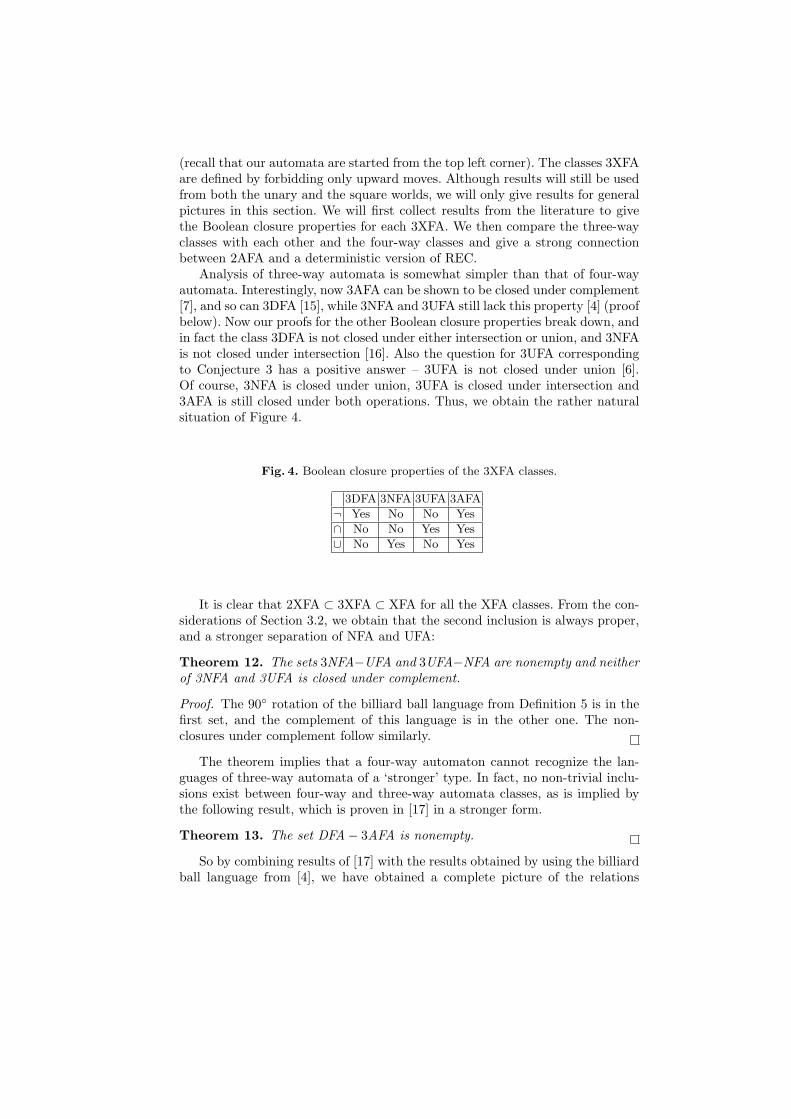
Analysis of three-way automata is somewhat simpler than that of four-wayautomata. Interestingly, now 3AFA can be shown to be closed under complement[7], and so can 3DFA [15], while 3NFA and 3UFA still lack this property [4] (proofbelow). Now our proofs for the other Boolean closure properties break down, andin fact the class 3DFA is not closed under either intersection or union, and 3NFAis not closed under intersection [16]. Also the question for 3UFA correspondingto Conjecture 3 has a positive answer – 3UFA is not closed under union [6].Of course, 3NFA is closed under union, 3UFA is closed under intersection and3AFA is still closed under both operations. Thus, we obtain the rather naturalsituation of Figure 4.

Fig. 4. Boolean closure properties of the 3XFA classes.

3DFA 3NFA 3UFA 3AFA

¬ Yes No No Yes

∩ No No Yes Yes

∪ No Yes No Yes

It is clear that 2XFA ⊂ 3XFA ⊂ XFA for all the XFA classes. From the con-siderations of Section 3.2, we obtain that the second inclusion is always proper,and a stronger separation of NFA and UFA:

Theorem 12. The sets 3NFA−UFA and 3UFA−NFA are nonempty and neitherof 3NFA and 3UFA is closed under complement.

Proof. The 90◦ rotation of the billiard ball language from Definition 5 is in thefirst set, and the complement of this language is in the other one. The non-closures under complement follow similarly.

The theorem implies that a four-way automaton cannot recognize the lan-guages of three-way automata of a ‘stronger’ type. In fact, no non-trivial inclu-sions exist between four-way and three-way automata classes, as is implied bythe following result, which is proven in [17] in a stronger form.

Theorem 13. The set DFA− 3AFA is nonempty.

So by combining results of [17] with the results obtained by using the billiardball language from [4], we have obtained a complete picture of the relations

between three- and four-way automata classes, on general pictures. We depictthis in Figure 5, where all inclusions are proper, all inclusions between classesare given by diagram chasing, and all other pairs of classes are incomparable.

Fig. 5. Diagram of inclusions for three-way and four-way automata classes.

3DFA

3NFA 3UFA

3AFA

DFA

NFA UFA

AFA

In Section 3.3, we showed some connections between REC and the XFAclasses (namely Theorems 4 and 5). It seems to be unknown whether co-AFAis actually equal to REC [7], although this seems unlikely. However, for 2-wayautomata, we have a natural connection between the two worlds: 2AFA is equalto a deterministic version of REC [18]. However, due to bad luck, the way theclasses are usually defined we have to rotate one of them by 180◦ to make themcoincide.

Definition 15. DREC is the subfamily of REC obtained by using north-westdeterministic tiles, that is, tilesets such that no two Wang tiles in the set mayshare both their north and west colors.

With the interpretation that REC accepts a language by assigning states onthe cells of a picture, this means when assigning states of a DREC grammar,knowing the north and west neighbors uniquely determines the state of thecurrent cell. We next prove the following [18]:

Theorem 14. 2AFAR = DREC.

We split the proof into two inclusions. Given a picture p and a position y, wedefine top left rectangle at y to be the rectangle between (1, 1) and y. Given sucha rectangle, we define its north child and west child as the rectangles that startfrom (1, 1) and end at y − (1, 0) and y − (0, 1), respectively. Note that 2AFAR

is of course just the class of languages accepted by 2-way AFA that start at thebottom right corner and can only move up and to the left.

Lemma 10. 2AFAR ⊆ DREC.

Proof. We construct a DREC grammar G simulating the given 2AFAR A. Ateach tile of G, the subset of states of A is held from which there is an accepting

computation of A for the top left rectangle at the position. At the top leftcorner, the correct subset of states of A is enforced, based on the symbol atthat position. It should be obvious how to inductively find the correct state setselsewhere, north-west deterministically, based on how the acceptance of an AFAis defined.

Lemma 11. DREC ⊆ 2AFAR.

Proof. Given a DREC grammar G, we find a 2AFAR A with the same language.The automaton A has the states T×S where T is the tileset of G, and S is a smallset of helper states needed in the construction (which we leave unspecified). Letus distinquish a state s ∈ S. When A is started in state (q, s) in cell x, it acceptsif and only if there is a consistent assignment of DREC states onto the cells ofthe top left rectangle at x such that the tile q is used as the state of cell x.

The top left corner can easily be detected by a 2AFAR. In the top left corner,A simply checks whether such a consistent assignment (of one tile) exists usinga look-up table. In the general case, A guesses the north and west neighbors q1and q2 of q with colors matching those of q. It then recursively checks these thatthe north and west children can be consistently colored in such a way that thecorresponding qi is used in the bottom right corner.

The algorithm works because in the recursion, in addition to consistent place-ments of states for the subpictures starting from the north and west neighborsexisting, they must also have the same tiles in the overlapping zone due to thedeterminism of DREC.

Then, the initial states of A simply start such searches from all tiles q ∈ T .

6 Markers

In this section, we only consider deterministic automata, and work on generalpictures. However, we give our automata a finite set of markers, which the au-tomaton can carry around, drop on the cells of the picture, and later lift upagain. The main results we present are from [1], although we will prove slightlystronger claims. There are many ways to formalize this idea, but most of thesecan be shown equivalent [1]. We choose the definition of ‘physical markers’, whichneed to be lifted before reusing, and which can be stacked on top of each other.

Of course, once k markers are given to our automata, we will obtain a hier-archy of languages based on how many markers are needed for a DFA to acceptthem. This hierarchy is proven infinite in [1] with a diagonalization argument. Wewill investigate only the beginning of this hierarchy, using concrete and naturalpicture languages.

The language Lcenter shows us DFA is already strengthened by the additionof one marker, since we can use the marker to implement essentially the same al-gorithm we used to prove Lcenter ∈ NFA. Denoting the class of picture languagesaccepted by DFA with n markers by nmDFA, we then have the following.

Theorem 15. DFA ( 1mDFA.

We will devote the main part of this section to separating DFA with twomarkers from those with just one, illustrating interesting programming tech-niques for DFA with markers, and an extended pigeonhole argument for DFAwith one marker.

Definition 16. For each n, Lnc is the language of pictures over {0, 1} contain-ing exactly n connected components over 1 (connected components of the graphwhere the vertices are the cells containing a 1, and there are edges between ad-jacent cells). We write Lc = L1c. For each n, we define Lneq as the subsetof Lnc containing exactly n components which are all translations of a singlecomponent.

In [1], in order to separate 1mDFA and 2mDFA, it is proven that there existsa language L ∈ 2mDFA whose intersection with L2c is exactly L2eq, but there isno such language in 1mDFA. We will instead prove the perhaps more interestingnew result that L2eq ∈ 2mDFA− 1mDFA.

The language Lc has been of interest to many authors in both the case ofpicture-walking automata and recognizability. In [19], Lc was proved to be inREC, while [17] proved it to be outside 3AFA. In [1], it was shown that a DFAcan accept Lc with one marker, and it was implicitly conjectured that this isnot possible with a regular DFA.

Conjecture 5. [1] The connected patterns are not in DFA.

Note that a proof through REC will certainly not work, since it is easyto write an AFA for Lc [20]. Neither does a direct pigeonhole argument seempossible.

Let us explain the construction of [1] for Lc with a one marker DFA, sinceit also nicely illustrates some of the techniques we will need for showing L2eq ∈2mDFA. First, we give some slightly informal terminology. By a local propertyP we mean a set of (p, x,m1, . . . ,mk), where x,mi ∈ dom(p), x representing thehead of the automaton and mi the positions of markers. We say P is an n-markerproperty, if a DFA with n unused markers started in cell x of picture p with somefixed k markers of its at m1, . . . ,mk can check whether (p, x,m1, . . . ,mk) ∈ P ,then returning to x carrying again the n markers.

So, let p ∈ Σ∗∗ be a binary picture. We say a column j of p is left separatingif it contains a 1, there is a 1 in p somewhere to the left of column j, and

6 ∃i : p[i, j] = 1 ∧ p[i, j − 1] = 1.

That is, left separating columns contain 1’s all of which are separated from all1’s to the left of them. Similarly, we define right separating columns. It is clearthat the 1’s of p are connected if and only if there are no left or right separatingcolumns, and on each column, two 1’s with only 0’s between them are connected.

Theorem 16. L1c ∈ 1mDFA.

Proof. Checking that no column is left or right separating is easy. Next, theautomaton reads the columns top-down, from left to right. At each 1 which isnot the last in its column, we check that it is in the same component as the next1 in the column. More precisely, we note that the local property ‘The current cellx contains a 1 and the next 1 in this column (at y) is in the same component.’ isa 1-marker property: the automaton drops the marker and then follows the edgeof the area of 1’s (using the classical labyrinth algorithm) until it either returnsto x, or it finds a 1 under the marker at x with only 0’s in between. Note thatthe latter is a 0-marker property and thus checkable during the search. In thefirst case, y is not in the same component, and we conclude p /∈ Lc. If the secondcase always occurs, we conclude p ∈ Lc.

We will first count that there are exactly two components, by extendingthe previous argument. This technique can be used to prove Lnc ∈ nmDFA,although, as in the case of one component, it is unknown whether this is optimal.

Theorem 17. L2c ∈ 2mDFA.

Proof. We define the shoulder of p as the cell containing a 1 seen first during acolumnwise top-down left to right search, and similarly we define the shoulderof a component of 1’s in p. We define the top left component as the componentof 1’s that the shoulder of p belongs to. Note that being on the outer border ofthe top left component is a 1-marker property, since whether the current cell isthe shoulder is a 0-marker property. For brevity, we call the top left componentA.

We now start a columnwise top-down left to right search over the picture.At each column, we continue down without permanently dropping any markers,while staying in A. This is possible since we can check whether the first cell wesee is in A (since it is necessarily on the outer border of its component), andwe can check whether the component changes as we move down the column. Ifanother component is not seen during the whole search, we conclude there isjust one component, and thus p /∈ L2c.

If a different component is seen at any time, we drop one of the markers.Note that it is then dropped at the outer border Y of some component B. Themarker will not be moved again, so in effect, whether a cell is on the outer borderof either A or B has turned into a 1-marker property. Just as importantly, if Bis completely within A, whether a cell belongs to the edge of the correspondinghole of A is now also a 1-marker property. Let X be the set of cells on this edge,or the outer border of A if B is not within A. We obtain that belonging to Xand belonging to Y are both one-marker properties.

After marking X and Y , we continue the search as previously, now essentiallywith a one marker automaton. When we enter the first component on a columnat x, we immediately conclude p /∈ L2c if this x is not in A or B (since, again,x is at the outer border of some component). After either A or B has beenentered, the automaton continues down the column while the component doesnot change. When it does change, we immediately reject if it does not go from Xto Y or from Y to X. If there are exactly two components, only such transitions

happen, and if only such transitions happen, A and B are of course the onlycomponents.

Next, let us compare these two components.

Theorem 18. L2eq ∈ 2mDFA.

Proof. By the previous theorem, we can assume there are exactly two compo-nents. Again, let A be the top left component and B the other one. Now, Bcannot be inside A or we can directly reject p. This is easy to check during theprevious algorithm, and even easier to do directly. Knowing this, we first locatethe shoulder of B: we do a columnwise search until either the first componentseen is not A or the component changes after a cell of A. We keep the othermarker – the B marker – here, and move the other marker to the shoulder ofA. The two markers will stay exactly this vector v away from each other duringthe rest of the search.

Now, consider the components as sets of vectors and p as the set of indiceswhere it contains a 1. We will check that A+v ⊂ p and B−v ⊂ p, which clearlyimplies A+v = B. For the first inclusion, we do a columnwise search using bothmarkers at once, and whenever the A-marker is in a cell of A, we check that theB-marker is on top of a 1. The second inclusion is done symmetrically.

In order to keep track of when the A-marker is on a cell of A, we start withthe markers at the shoulders of the corresponding components. Both markersare moved down simultaneously while the A-marker stays within A, skipping 0’sin the usual way, and we check the B-marker is on top of a 1 whenever the A-marker is. When the A-marker changes component, the head must have enteredB. We then continue until the component changes again: we must have returnedto A, and the search continues normally.

Now, let us prove also the negative result – that two markers are in factnecessary for L2eq.

Theorem 19. L2eq /∈ 1mDFA

Proof. Suppose A is a 1mDFA with L(A) = L2eq and let A have k states. Weassume A directly returns to the domain of the picture if it enters its border.

We will use a similar argument as the one in the proof of Theorem 3. For eachpicture p we define the function fp mapping ‘incoming ID’s’ to ‘outgoing ID’s’,although this time we also allow ‘accept’, ‘reject’ and ‘loop’ in the codomain.(We could avoid this by repeating the argument of [10] for one-marker DFA.)The function fp completely characterizes the behavior of A on p as long as theautomaton enters the picture without carrying the marker. We say that twopictures p and q are A-equivalent if fp = fq.

The basic idea for applying the pigeonhole principle here is that while themarker stays on one side of the picture, the original partition into A-equivalentpictures applies to the other side, and the marker cannot be moved across themiddle of the picture more than a linear amount of times without the automatonentering a cycle. Let us make this idea more precise.

Let n be fixed, and let X be the set of all pictures of size n × n containingexactly one connected component with 0’s around it. To each element of X2 wenaturally associate a picture of shape n × 2n where the two elements of X aresimply concatenated (note that such a picture is in L2c). The left- and right-hand sides of these pictures p are called the LHS and the RHS. We will showthat for large enough n, A will accept all pictures in Y × Y for some subset Yof X with more than one element, which is a contradiction.

We note that for some n-independent D, |X| ≥ 2Dn2

for large enough nby using a suitable skeleton of 1’s to allow rows on which bits can be chosenfreely while keeping the pattern connected. Let P be the partition of X intoA-equivalence classes, and again note that there are at most CnCn componentsin P for some C depending only on A. We write X/P for a maximal subset Zof X containing only A-equivalent elements (tie-breaking in some natural way).Of course, |Z| ≥ |X||P | .

Let us restrict our attention to Y0 = X/P . Consider the pictures Y 20 . The

automaton cannot accept any of the pictures in this set without moving themarker on the right side, since the RHS are all A-equivalent. For some subsetY ′0 ⊂ Y0 of size at least |Y0|

kn , A exits the LHS with the marker the first timethe same way in all pictures of Y ′0

2. Note that the content of the RHS does notinfluence how the marker leaves the LHS, since all pictures in Y0 are A-equivalent.If Y ′0 has more than one element, A must eventually move the marker back tothe LHS. Again, it does this the same way on some subset Y1 ⊂ Y ′0 of size |Y

′0 |kn .

If Y1 has more than one element, the marker eventually has to be moved onthe right side, but now this can be done in only kn − 1 ways, since otherwisethe automaton enters an infinite loop on all pictures of Y 2

1 , which is impossiblebecause Y 2

1 ∩L2eq 6= ∅. We thus obtain sets Y ′1 and Y2, and similarly Y ′i and Yi+1

for all i until the size of one of these reaches 0 or 1. Note that |Yi+1| ≥ |Yi|(kn−i)2 .

Since the automaton necessarily loops when i reaches kn, we have obtained|X/P | ≤ (kn)!2. But we can show this is false for large enough n, using astandard argument:

2Dn2

CnCn(kn)!2≤ |X/P |

(kn)!2≤ 1 ⇐⇒

Dn2 − Cn logCn− 2 log(kn)! ≤ log|X/P |(kn)!2

≤ 0

which is clearly not the case, using String’s approximation for log(kn)!. This isa contradiction, and thus L2eq /∈ 1mDFA.

Corollary 6. 1mDFA ( 2mDFA.

7 Algorithmic questions

Picture walking automata admit efficient parsing of pictures. Pictures of a lan-guage can be recognized in linear time on the size n = |p| × p of the picturep.

In the case of DFA, the linear time recognition can be done using logarithmicspace: By Theorem 1 we can assume the DFA halts on every input picture so itis enough to run the DFA until it halts. This happens within O(n) steps, andduring the computation one stores the current state and position of the DFAusing O(log n) space.

In the cases of NFA, UFA and AFA, linear space is enough. Consider thedirected graph whose vertices are the instantaneous descriptions (q, x) of theautomaton, and edges are given by the successor relation l1 −→ l2. For NFA,picture recognition amounts to finding a path from an initial ID to an acceptingID, which can be solved using standard depth-first search. In AFA, the verticesare classified as universal and existential. A simple linear-time algorithm executesa DFS search from the final ID’s backwards, progressively marking new verticesthat lead to acceptance. A universal vertex is marked only when all its followersbecome marked, while for existential vertices it is enough to have one followermarked. A picture is in the language iff an initial ID gets marked.

Another family of algorithmic questions concern the languages recognized bygiven automata. Here the situation is quite different, and undecidability usuallyprevails. The basic question is the emptiness problem: does the given automatonaccept any pictures ? It was mentioned already in [1] that unary emptiness forDFA is undecidable because Minsky machines can be simulated. Recall thatMinsky’s two-counter machine without an input tape consists of a deterministicfinite automaton and two counters, each storing one non-negative integer. Themachine can detect when either counter is zero. The machine changes its stateaccording to a deterministic transition rule. The new state only depends on theold state and on the results of the tests that check whether either counter isequal to zero. The transition rule also specifies whether to increment, decrementor keep unchanged the counters.

It is well known that two-counter machines can simulate Turing machines [21].In particular, it is undecidable whether a given machine reaches a specified halt-ing state h when started in its initial state i with both counters initialized tovalue 0.

A 2-counter machine can be interpreted as a DFA that operates on the (infi-nite) quadrant of the plane and has the same finite states as the 2-counter ma-chine. The position of the DFA encodes the two counter values: Position (x, y)represents counter values x and y. Increments and decrements of the counterscorrespond to horizontal and vertical steps of the DFA on the plane.

Any computation of a 2-counter machine can therefore be simulated by aDFA inside a sufficiently large rectangle. The dimensions of the rectangle haveto be at least as large as the largest counter values used during the acceptingcomputation. Zero values of the counters can be recognized as these correspondto the machine stepping on the top or left boundary of the rectangle. If the DFAtries to step on the right or the bottom border, it enters an error state e thatindicates that the rectangle was not large enough.

It is clear that the DFA outlined above accepts exactly the rectangles of sizesw × h where w and h are greater than the largest values in the two counters,

respectively, used during the accepting run of the Minsky machine. If the Minskymachine does not halt, the DFA does not accept any rectangle. Hence we havethe following.

Theorem 20. It is undecidable if a given unary DFA accepts any rectangles [1].

In the restricted models the situation is more interesting, and various de-cidability questions have been investigated among three-way automata [22–24].In [22], the unary emptiness was shown to be decidable among 3NFA, and in [24]the result was extended to arbitrary alphabets. It was also shown in [24] thatunary emptiness is undecidable among 3AFA, and even among 2AFA.

Theorem 21. The emptiness problem is

– decidable among 3NFA [22, 24],– undecidable among unary 2AFA [24].

Finally, we mention another application of the Minsky machine simulationby DFA, stating that the sizes of unary squares recognized by DFA can form avery sparse set [9].

Theorem 22. Let {a1, a2, . . .} be any recursively enumerable set of positive in-tegers. There exists a DFA that recognizes the language of unary squares of sizesbi × bi for i = 1, 2, . . . where bi > ai for all i = 1, 2, . . ..

The theorem is proved easily using the DFA simulation of a two-countermachine. First, an NFA is build where non-determinism is used to select theinitial counter values for the Minsky machine. Such limited non-determinismcan then be removed using the trick from [10]. See [9] for the details.

8 Conclusions

To conclude, we collect the open problems from the text into a single list.

Conjecture 1 The language of unary squares with prime side length are not inDFA.

Conjecture 2 DFA is a proper subset of NFA when restricted to unary squares.

Conjecture 3 UFA is not closed under union.

Conjecture 4 NFA = FNFA on three-dimensional pictures.

Conjecture 5 The connected patterns are not in DFA.

9 Acknowledgements

We would like to thank Ilkka Torma for helpful remarks on marker automata,and for reviewing the section on them.

References

1. Blum, M., Hewitt, C.: Automata on a 2-dimensional tape. In: FOCS, IEEE (1967)155–160

2. Inoue, K., Takanami, I.: A survey of two-dimensional automata theory. Inf. Sci.55(1-3) (1991) 99–121

3. Giammarresi, D., Restivo, A. In: Two-dimensional languages. Springer-Verlag NewYork, Inc., New York, NY, USA (1997) 215–267

4. Kari, J., Moore, C.: New results on alternating and non-deterministic two-dimensional finite-state automata. In Ferreira, A., Reichel, H., eds.: STACS. Vol-ume 2010 of Lecture Notes in Computer Science., Springer (2001) 396–406

5. Salo, V.: Classes of picture languages defined by tiling systems, automata andclosure properties. Master’s thesis, University of Turku (2011)

6. Ito, A., Inoue, K., Takanami, I., Taniguchi, H.: Two-dimensional alternating turingmachines with only universal states. Information and Control 55(1-3) (1982) 193–221

7. Ibarra, O.H., Jiang, T., 0008, H.W.: Some results concerning 2-d on-line tessellationacceptors and 2-d alternating finite automata. In: MFCS. (1991) 221–230

8. Okazaki, T., Zhang, L., Inoue, K., Ito, A., 0002, Y.W.: A note on two-dimensionalprobabilistic finite automata. Inf. Sci. 110(3-4) (1998) 303–314

9. Kari, J., Moore, C.: Rectangles and squares recognized by two-dimensional au-tomata. In Karhumaki, J., Maurer, H.A., Paun, G., Rozenberg, G., eds.: TheoryIs Forever. Volume 3113 of Lecture Notes in Computer Science., Springer (2004)134–144

10. Sipser, M.: Halting space-bounded computations. In: FOCS, IEEE (1978) 73–7411. Rosenfeld, A.: Picture Languages: Formal Models for Picture Recognition. Aca-

demic Press, Inc., Orlando, FL, USA (1979)12. Lindgren, K., Moore, C., Nordahl, M.: Complexity of two-dimensional patterns.

Journal of Statistical Physics 91 (1998) 909–951 10.1023/A:1023027932419.13. Ladner, R.E., Lipton, R.J., Stockmeyer, L.J.: Alternating pushdown and stack

automata. SIAM J. Comput. 13(1) (1984) 135–15514. Parikh, R.: On context-free languages. J. ACM 13(4) (1966) 570–58115. Szepietowski, A.: Some remarks on two-dimensional finite automata. Inf. Sci.

63(1-2) (1992) 183–18916. Inoue, K., Takanami, I.: Three-way tape-bounded two-dimensional turing ma-

chines. Inf. Sci. 17(3) (1979) 195–22017. Ito, A., Inoue, K., Takanami, I.: A note on three-way two-dimensional alternating

turing machines. Inf. Sci. 45(1) (1988) 1–2218. Ito, A., Inoue, K., Takanami, I.: Deterministic two-dimensional on-line tessellation

acceptors are equivalent to two-way two-dimensional alternating finite automatathrough 180-rotation. Theor. Comput. Sci. 66(3) (1989) 273–287

19. Reinhardt, K.: On some recognizable picture-languages. In Brim, L., Gruska, J.,Zlatuska, J., eds.: MFCS. Volume 1450 of Lecture Notes in Computer Science.,Springer (1998) 760–770

20. Inoue, K., Takanami, I., Taniguchi, H.: Two-dimensional alternating turing ma-chines. Theor. Comput. Sci. 27 (1983) 61–83

21. Minsky, M.L.: Computation: finite and infinite machines. Prentice-Hall, Inc. (1967)22. Inoue, K., Takanami, I.: A note on decision problems for three-way two-dimensional

finite automata. Inf. Process. Lett. 10(4/5) (1980) 245–24823. Kinber, E.B.: Three-way automata on rectangular tapes over a one-letter alphabet.

Inf. Sci. 35(1) (1985) 61–7724. Petersen, H.: Some results concerning two-dimensional turing machines and finite

automata. In Reichel, H., ed.: FCT. Volume 965 of Lecture Notes in ComputerScience., Springer (1995) 374–382