a survey on tree edit distance and related problems
TRANSCRIPT
A Survey on Tree Edit Distance and Related
Problems
Philip Bille∗
The IT University of Copenhagen
Glentevej 67, DK-2400 Copenhagen NV, Denmark.
Email: [email protected].
Abstract
We survey the problem of comparing labeled trees based on simple
local operations of deleting, inserting, and relabeling nodes. These op-
erations lead to the tree edit distance, alignment distance, and inclusion
problem. For each problem we review the results available and present,
in detail, one or more of the central algorithms for solving the problem.
keywords tree matching, edit distance
1 Introduction
Trees are among the most common and well-studied combinatorial structures incomputer science. In particular, the problem of comparing trees occurs in severaldiverse areas such as computational biology, structured text databases, imageanalysis, automatic theorem proving, and compiler optimization [43, 55, 22, 24,16, 35, 56]. For example, in computational biology, computing the similaritybetween trees under various distance measures is used in the comparison ofRNA secondary structures [55, 18].
Let T be a rooted tree. We call T a labeled tree if each node is a assigned asymbol from a fixed finite alphabet Σ. We call T an ordered tree if a left-to-rightorder among siblings in T is given. In this paper we consider matching problemsbased on simple primitive operations applied to labeled trees. If T is an orderedtree these operations are defined as follows:
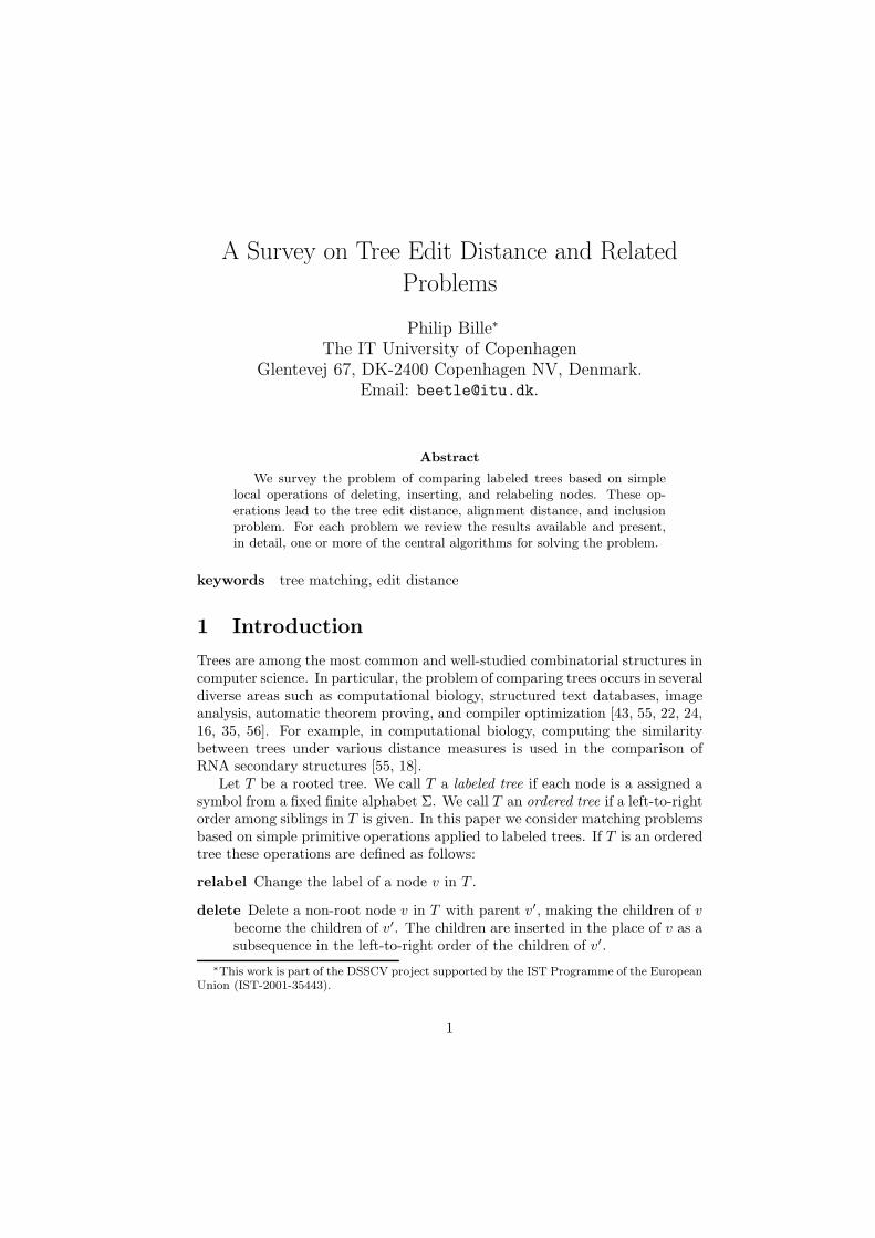
relabel Change the label of a node v in T .
delete Delete a non-root node v in T with parent v′, making the children of v
become the children of v′. The children are inserted in the place of v as asubsequence in the left-to-right order of the children of v′.
∗This work is part of the DSSCV project supported by the IST Programme of the EuropeanUnion (IST-2001-35443).
1
(a) l1 l2
(b) l1 l1
l2
(b) l1 l1
l2
Figure 1: (a) A relabeling of the node label l1 to l2. (b) Deleting the nodelabeled l2. (c) Inserting a node labeled l2 as the child of the node labeled l1.
insert The complement of delete. Insert a node v as a child of v′ in T makingv the parent of a consecutive subsequence of the children of v′.
Figure 1 illustrates the operations. For unordered trees the operations can bedefined similarly. In this case, the insert and delete operations works on asubset instead of a subsequence. We define three problems based on the editoperations. Let T1 and T2 be labeled trees (ordered or unordered).
Tree edit distance Assume that we are given a cost function defined oneach edit operation. An edit script S between T1 and T2 is a sequence of editoperations turning T1 into T2. The cost of S is the sum of the costs of theoperations in S. An optimal edit script between T1 and T2 is an edit scriptbetween T1 and T2 of minimum cost and this cost is the tree edit distance. Thetree edit distance problem is to compute the edit distance and a correspondingedit script.
2

Tree alignment distance Assume that we are given a cost function definedon pair of labels. An alignment A of T1 and T2 is obtained as follows. First weinsert nodes labeled with spaces into T1 and T2 so that they become isomorphicwhen labels are ignored. The resulting trees are then overlayed on top of eachother giving the alignment A, which is a tree where each node is labeled by apair of labels. The cost of A is the sum of costs of all pairs of opposing labelsin A. An optimal alignment of T1 and T2 is an alignment of minimum cost andthis cost is called the alignment distance of T1 and T2. The alignment distanceproblem is to compute the alignment distance and a corresponding alignment.
Tree inclusion T1 is included in T2 if and only if T1 can be obtained bydeleting nodes from T2. The tree inclusion problem is to determine if T1 isincluded in T2.
In this paper we survey each of these problems and discuss the results ob-tained for them. For reference, Table 1 on page 27 summarizes most of theavailable results. All of these and a few others are covered in the text. Thetree edit distance problem is the most general of the problems. The alignmentdistance corresponds to a kind of restricted edit distance, while tree inclusionis a special case of both the edit and alignment distance problem. Apart fromthese simple relationships, interesting variations on the edit distance problemhas been studied leading to a more complex picture.
Both the ordered and unordered version of the problems are reviewed. Forthe unordered case, it turns out that all of the problems in general are NP-hard.Indeed, the tree edit distance and alignment distance problems are even MAXSNP-hard [4]. However, under various interesting restrictions, or for specialcases, polynomial time algorithms are available. For instance, if we impose astructure preserving restriction on the unordered tree edit distance problem,such that disjoint subtrees are mapped to disjoint subtrees, it can be solved inpolynomial time. Also, unordered alignment for constant degree trees can besolved efficiently.
For the ordered version of the problems polynomial time algorithms exists.These are all based on the classic technique of dynamic programming (see, e.g.,[9, Chapter 15]) and most of them are simple combinatorial algorithms. Recentlyhowever, more advanced techniques such as fast matrix multiplication have beenapplied to the tree edit distance problem [8].
The survey covers the problems in the following way. For each problem andvariations of it we review results for both the ordered and unordered version.This will in most cases include a formal definition of the problem, a comparisonof the available results and a description of the techniques used to obtain theresults. More importantly, we will also pick one or more of the central algorithmsfor each of the problems and present it in almost full detail. Specifically, we willdescribe the algorithm, prove that it is correct, and analyze its time complexity.For brevity, we will omit the proofs of a few lemmas and skip over some lessimportant details. Common for the algorithms presented in detail is that, inmost cases, they are the basis for more advanced algorithms. Typically, most
3

of the algorithms for one of the above problems are refinements of the samedynamic program.
The main technical contribution of this survey is to present the problemsand algorithms in a common framework. Hopefully, this will enable the readerto gain a better overview and deeper understanding of the problems and howthey relate to each other. In the literature, there are some discrepancies in thepresentations of the problems. For instance, the ordered edit distance problemwas considered by Klein [25] who used edit operations on edges. He presentedan algorithm using a reduction to a problem defined on balanced parenthesisstrings. In contrast, Zhang and Shasha [55] gave an algorithm based on thepostorder numbering on trees. In fact, these algorithms share many featureswhich become apparent if considered in the right setting. In this paper wepresent these algorithms in a new framework bridging the gap between the twodescriptions.
Another problem in the literature is the lack of an agreement on a definitionof the edit distance problem. The definition given here is by far the most studiedand in our opinion the most natural. However, several alternatives ending invery different distance measures have been considered [30, 45, 38, 31]. In thispaper we review these other variants and compare them to our definition. Weshould note that the edit distance problem defined here is sometimes referredto as the tree-to-tree correction problem.
This survey adopts a theoretical point of view. However, the problems aboveare not only interesting mathematical problems but they also occur in manypractical situations and it is important to develop algorithms that perform wellon real-life problems. For practical issues see, e.g., [49, 46, 40].
We restrict our attention to sequential algorithms. However, there has beensome research in parallel algorithms for the edit distance problem, e.g., [55, 53,41].
This summarizes the contents of this paper. Due to the fundamental natureof comparing trees and its many applications several other ways to comparetrees have been devised. In this paper, we have chosen to limit ourselves to ahandful of problems which we describe in detail. Other problems include treepattern matching [27, 10] and [16, 35, 56], maximum agreement subtree [19, 11],largest common subtree [2, 20], and smallest common supertree [34, 13].
1.1 Outline
In Section 2 we give some preliminaries. In Sections 3, 4, and 5 we survey thetree edit distance, alignment distance, and inclusion problems respectively. Weconclude in Section 6 with some open problems.
2 Preliminaries and notation
In this section we define notations and definitions we will use throughout thepaper. For a graph G we denote the set of nodes and edges by V (G) and E(G)
4

respectively. Let T be a rooted tree. The root of T is denoted by root(T ). Thesize of T , denoted by |T |, is |V (T )|. The depth of a node v ∈ V (T ), depth(v),is the number of edges on the path from v to root(T ). The in-degree of a nodev, deg(v) is the number of children of v. We extend these definitions such thatdepth(T ) and deg(T ) denotes the maximum depth and degree respectively ofany node in T . A node with no children is a leaf and otherwise an internalnode. The number of leaves of T is denoted by leaves(T ). We denote the parentof node v by parent(v). Two nodes are siblings if they have the same parent.For two trees T1 and T2, we will frequently refer to leaves(Ti), depth(Ti), anddeg(Ti) by Li, Di, and Ii, i = 1, 2.
Let θ denote the empty tree and let T (v) denote the subtree of T rootedat a node v ∈ V (T ). If w ∈ V (T (v)) then v is an ancestor of w, and if w ∈V (T (v))\{v} then v is a proper ancestor of w. If v is a (proper) ancestor of w
then w is a (proper) descendant of v. A tree T is ordered if a left-to-right orderamong the siblings is given. For an ordered tree T with root v and childrenv1, . . . , vi, the preorder traversal of T (v) is obtained by visiting v and thenrecursively visiting T (vk), 1 ≤ k ≤ i, in order. Similarly, the postorder traversalis obtained by first visiting T (vk), 1 ≤ k ≤ i, and then v. The preorder numberand postorder number of a node w ∈ T (v), denoted by pre(w) and post(w), isthe number of nodes preceding w in the preorder and postorder traversal of T
respectively. The nodes to the left of w in T is the set of nodes u ∈ V (T ) suchthat pre(u) < pre(w) and post(u) < post(w). If u is to the left of w then w isto the right of u.
A forest is a set of trees. A forest F is ordered if a left-to-right order amongthe trees is given and each tree is ordered. Let T be an ordered tree and letv ∈ V (T ). If v has children v1, . . . , vi define F (vs, vt), where 1 ≤ s ≤ t ≤ i, asthe forest T (vs), . . . , T (vr). For convenience, we set F (v) = F (v1, vi).
We assume throughout the paper that labels assigned to nodes are chosenfrom a finite alphabet Σ. Let λ 6∈ Σ denote a special blank symbol and defineΣλ = Σ∪λ. We often define a cost function, γ : (Σλ ×Σλ)\(λ, λ) → R, on pairsof labels. We will always assume that γ is a distance metric. That is, for anyl1,l2,l3 ∈ Σλ the following conditions are satisfied:
1. γ(l1, l2) ≥ 0, γ(l1, l1) = 0.
2. γ(l1, l2) = γ(l2, l1).
3. γ(l1, l3) ≤ γ(l1, l2) + γ(l2, l3).
3 Tree Edit Distance
In this section we survey the tree edit distance problem. Assume that we aregiven a cost function defined on each edit operation. An edit script S betweentwo trees T1 and T2 is a sequence of edit operations turning T1 into T2. Thecost of S is the sum of the costs of the operations in S. An optimal edit scriptbetween T1 and T2 is an edit script between T1 and T2 of minimum cost. This
5

f f a
d e d e c d
a
c
a b
d
b a b
(a) (b) (c)
Figure 2: Transforming (a) into (c) via editing operations. (a) A tree. (b) Thetree after deleting the node labeled c. (c) The tree after inserting the nodelabeled c and relabeling f to a and e to d.
cost is called the tree edit distance, denoted by δ(T1, T2). An example of an editscript is shown in Figure 2.
The rest of the section is organized as follows. First, in Section 3.1, wepresent some preliminaries and formally define the problem. In Section 3.2 wesurvey the results obtained for the ordered edit distance problem and presenttwo of the currently best algorithms for the problem. The unordered versionof the problem is reviewed in Section 3.3. In Section 3.4 we review resultson the edit distance problem when various structure-preserving constraints areimposed. Finally, in Section 3.5 we consider some other variants of the problem.
3.1 Edit operations and edit mappings
Let T1 and T2 be labeled trees. Following [43] we represent each edit operationby (l1 → l2), where (l1, l2) ∈ (Σλ × Σλ)\(λ, λ). The operation is a relabeling ifl1 6= λ and l2 6= λ, a deletion if l2 = λ, and an insertion if l1 = λ. We extend thenotation such that (v → w) for nodes v and w denotes (label(v) → label(w)).Here, as with the labels, v or w may be λ. Given a metric cost function γ
defined on pairs of labels we define the cost of an edit operation by settingγ(l1 → l2) = γ(l1, l2). The cost of a sequence S = s1, . . . , sk of operations is
given by γ(S) =∑k
i=1 γ(si). The edit distance, δ(T1, T2), between T1 and T2 isformally defined as:
δ(T1, T2) = min{γ(S) | S is a sequence of operations transforming T1 into T2}.
Since γ is a distance metric δ becomes a distance metric too.An edit distance mapping (or just a mapping) between T1 and T2 is a rep-
resentation of the edit operations, which is used in many of the algorithms forthe tree edit distance problem. Formally, define the triple (M, T1, T2) to be anordered edit distance mapping from T1 to T2, if M ⊆ V (T1)×V (T2) and for anypair (v1, w1), (v2, w2) ∈ M :
1. v1 = v2 iff w1 = w2. (one-to-one condition)
6

f a
d e c d
a
c d
b a b
Figure 3: The mapping corresponding to the edit script in Figure 2.
2. v1 is an ancestor of v2 iff w1 is an ancestor of w2. (ancestor condition)
3. v1 is to the left of v2 iff w1 is to the left of w2. (sibling condition)
Figure 3 illustrates a mapping that corresponds to the edit script in Figure 2. Wedefine the unordered edit distance mapping between two unordered trees as thesame, but without the sibling condition. We will use M instead of (M, T1, T2)when there is no confusion. Let (M, T1, T2) be a mapping. We say that a nodev in T1 or T2 is touched by a line in M if v occurs in some pair in M . Let N1
and N2 be the set of nodes in T1 and T2 respectively not touched by any line inM . The cost of M is given by:
γ(M) =∑
(v,w)∈M
γ(v → w) +∑
v∈N1
γ(v → λ) +∑
w∈N2
γ(λ → w)
Mappings can be composed. Let T1, T2, and T3 be labeled trees. Let M1 andM2 be a mapping from T1 to T2 and T2 to T3 respectively. Define
M1 ◦ M2 = {(v, w) | ∃u ∈ V (T2) such that (v, u) ∈ M1 and (u, w) ∈ M2}
With this definition it follows easily that M1 ◦ M2 itself becomes a mappingfrom T1 to T3. Since γ is a metric, it is not hard to show that a minimum costmapping is equivalent to the edit distance:
δ(T1, T2) = min{γ(M) | (M, T1, T2) is an edit distance mapping}.
Hence, to compute the edit distance we can compute the minimum costmapping. We extend the definition of edit distance to forests. That is, for twoforests F1 and F2, δ(F1, F2) denotes the edit distance between F1 and F2. Theoperations are defined as in the case of trees, however, roots of the trees in theforest may now be deleted and trees can be merged by inserting a new root.The definition of a mapping is extended in the same way.
3.2 General ordered edit distance
The ordered edit distance problem was introduced by Tai [43] as a general-ization of the well-known string edit distance problem [48]. Tai presented an
7
algorithm for the ordered version using O(|T1||T2||L1|2|L2|
2) time and space.Subsequently, Zhang and Shasha [55] gave a simple algorithm improving thebounds to O(|T1||T2|min(L1, D1)min(L2, D2)) time and O(|T1||T2|) space. Thisalgorithm was modified by Klein [25] to get a better worst case time bound ofO(|T1|
2|T2| log |T2|)1 under the same space bounds. We present the latter two
algorithms in detail below. Recently, Chen [8] has presented an algorithm usingO(|T1||T2|+ L2
1|T2|+ L2.51 L2) time and O((|T1|+ L2
1)min(L2, D2) + |T2|) space.Hence, for certain kinds of trees the algorithm improves the previous bounds.This algorithm is more complex than all of the above and uses results on fastmatrix multiplication. Note that in the above bounds we can exchange T1 withT2 since the distance is symmetric.
3.2.1 A simple algorithm
We first present a simple recursion which will form the basis for the two dynamicprogramming algorithms we present in the next two sections. We will only showhow to compute the edit distance. The corresponding edit script can be easilyobtained within the same time and space bounds. The algorithm is due to Klein[25]. However, we should note that the presentation given here is somewhatdifferent. We believe that our framework is more simple and provides a betterconnection to previous work.
Let F be a forest and v be a node in F . We denote by F − v the forestobtained by deleting v from F . Furthermore, define F − T (v) as the forestobtained by deleting v and all descendants of v. The following lemma providesa way to compute edit distances for the general case of forests.
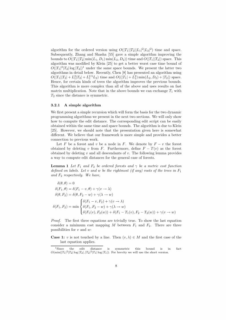
Lemma 1 Let F1 and F2 be ordered forests and γ be a metric cost functiondefined on labels. Let v and w be the rightmost (if any) roots of the trees in F1
and F2 respectively. We have,
δ(θ, θ) = 0
δ(F1, θ) = δ(F1 − v, θ) + γ(v → λ)
δ(θ, F2) = δ(θ, F2 − w) + γ(λ → w)
δ(F1, F2) = min
δ(F1 − v, F2) + γ(v → λ)
δ(F1, F2 − w) + γ(λ → w)
δ(F1(v), F2(w)) + δ(F1 − T1(v), F2 − T2(w)) + γ(v → w)
Proof. The first three equations are trivially true. To show the last equationconsider a minimum cost mapping M between F1 and F2. There are threepossibilities for v and w:
Case 1: v is not touched by a line. Then (v, λ) ∈ M and the first case of thelast equation applies.
1Since the edit distance is symmetric this bound is in factO(min(|T1|2|T2| log |T2|, |T2|2|T1| log |T1|). For brevity we will use the short version.
8

Case 2: w is not touched by a line. Then (λ, w) ∈ M and the second case ofthe last equation applies.
Case 3: v and w are both touched by lines. We show that this implies (v, w) ∈M . Suppose (v, h) and (k, w) are in M . If v is to the right of k then h
must be to right of w by the sibling condition. If v is a proper ancestor ofk then h must be a proper ancestor of w by the ancestor condition. Bothof these cases are impossible since v and w are the rightmost roots andhence (v, w) ∈ M . By the definition of mappings the equation follows. �
Lemma 1 suggests a dynamic program. The value of δ(F1, F2) depends ona constant number of subproblems of smaller size. Hence, we can computeδ(F1, F2) by computing δ(S1, S2) for all pairs of subproblems S1 and S2 in orderof increasing size. Each new subproblem can be computed in constant time.Hence, the time complexity is bounded by the number of subproblems of F1
times the number of subproblems of F2.To count the number of subproblems, define for a rooted, ordered forest F
the (i, j)-deleted subforest, 0 ≤ i + j ≤ |F |, as the forest obtained from F byfirst deleting the rightmost root repeatedly j times and then, similarly, deletingthe leftmost root i times. We call the (0, j)-deleted and (i, 0)-deleted subforests,for 0 ≤ j ≤ |F |, the prefixes and the suffixes of F respectively. The number
of (i, j)-deleted subforests of F is∑|F |
k=0 k = O(|F |2), since for each i there are|F | − i choices for j.
It is not hard to show that all the pairs of subproblems S1 and S2 that canbe obtained by the recursion of Lemma 1 are deleted subforests of F1 and F2.Hence, by the above discussion the time complexity is bounded by O(|F1|
2|F2|2).
In fact, fewer subproblems are needed, which we will show in the next sections.
3.2.2 Zhang and Shasha’s algorithm
The following algorithm is due to Zhang and Shasha [55]. Define the keyrootsof a rooted, ordered tree T as follows:
keyroots(T ) = {root(T )} ∪ {v ∈ V (T ) | v has a left sibling}
The special subforests of T is the forests F (v), where v ∈ keyroots(T ). Therelevant subproblems of T with respect to the keyroots is the prefixes of all specialsubforests F (v). In this section we refer to these as just the relevant subproblems.
Lemma 2 For each node v ∈ V (T ), F (v) is a relevant subproblem.
It is easy to see that, in fact, the subproblems that can occur in the aboverecursion are either subforests of the form F (v), where v ∈ V (T ), or prefixesof a special subforest of T . Hence, it follows by Lemma 2 and the definitionof a relevant subproblem, that to compute δ(F1, F2) it is sufficient to computeδ(S1, S2) for all relevant subproblems S1 and S2 of T1 and T2 respectively.
9

The relevant subproblems of a tree T can be counted as follows. For a nodev ∈ V (T ) define the collapsed depth of v, cdepth(v), as the number of keyrootancestors of v. Also, define cdepth(T ) as the maximum collapsed depth of allnodes v ∈ V (T ).
Lemma 3 For an ordered tree T the number of relevant subproblems, with re-spect to the keyroots is bounded by O(|T |cdepth(T )).
Proof. The relevant subproblems can be counted using the following expression:
∑
v∈keyroots(T )
|F (v)| <∑
v∈keyroots(T )
|T (v)| =∑
v∈V (T )
cdepth(v) ≤ |T |cdepth(T )
Since the number prefixes of a subforest F (v) is |F (v)| the first sum counts thenumber of relevant subproblems of F (v). To prove the first equality note thatfor each node v the number of special subforests containing v is the collapseddepth of v. Hence, v contributes the same amount to the left and right side.The other equalities/inequalities follow immediately. �
Lemma 4 For a tree T , cdepth(T ) ≤ min{depth(T ), leaves(T )}
Thus, using dynamic programming it follows that the problem can be solved intime (and space) O(|T1||T2|min{D1, L1}min{D2, L2}). Furthermore, by care-fully discarding distances between prefixes of special forests the space used inthe computation can be reduced to O(|T1||T2|). Hence,
Theorem 1 ([55]) For ordered trees T1 and T2 the edit distance problem canbe solved in time O(|T1||T2|min{D1, L1}min{D2, L2}) and space O(|T1||T2|).
3.2.3 Klein’s algorithm
In the worst case, that is for trees with linear depth and a linear numberof leaves, Zhang and Shasha’s algorithm of the previous section still requiresO(|T1|
2|T2|2) time as the simple algorithm. In [25] Klein obtained a better worst
case time bound of O(|T1|2|T2| log |T2|) while maintaining the same space bound
of O(|T1||T2|). It should be noted that the paper only states O(|T1|2|T2| log |T2|)
as the space bound. However, it is straightforward to improve this to O(|T1||T2|)[23].
The algorithm is based on an extension of the recursion in Lemma 1. Themain idea is to consider all of the O(|T1|
2) deleted subforests of T1 but onlyO(|T2| log |T2|) deleted subforests of T2. In total the worst case number ofsubproblems is thus reduced to the desired bound above.
A key concept in the algorithm is the decomposition of a rooted tree T intodisjoint paths called heavy paths. This technique was introduced by Harel andTarjan [15]. We define the size a node v ∈ V (T ) as |T (v)|. We classify eachnode of T as either heavy or light as follows. The root is light. For each internalnode v we pick a child u of v of maximum size among the children of v and
10

classify u as heavy. The remaining children are light. We call an edge to a lightchild a light edge, and an edge to a heavy child a heavy edge. The light depthof a node v, ldepth(v), is the number of light edges on the path from v to theroot.
Lemma 5 ([15]) For any tree T and any v ∈ V (T ), ldepth(v) ≤ log |T |+O(1).
By removing the light edges T is partitioned into heavy paths.We define the relevant subproblems of T with respect to the light nodes below.
We will refer to these as relevant subproblems in this section. First fix a heavypath decomposition of T . For a node v in T we recursively define the relevantsubproblems of F (v) as follows: F (v) is relevant. If v is not a leaf, let u bethe heavy child of v and let l and r be the number of nodes to the left and tothe right of u in F (v) respectively. Then, the (i, 0)-deleted subforests of F (v),0 ≤ i ≤ l, and the (l, j)-deleted subforests of F (v), 0 ≤ j ≤ r are relevantsubproblems. Recursively, all relevant subproblems of F (u) are relevant.
The relevant subproblems of T with respect to the light nodes is the unionof all relevant subproblems of F (v) where v ∈ V (T ) is a light node.
Lemma 6 For an ordered tree T the number of relevant subproblems with re-spect to the light nodes is bounded by O(|T | ldepth(T )).
Proof. Follows by the same calculation as in the proof of Lemma 3. �
Also note that Lemma 2 still holds with this new definition of relevant sub-problems. Let S be a relevant subproblem of T and let vl and vr denote theleftmost and rightmost root of S respectively. The difference node of S is eithervr if S−vr is relevant or vl if S−vl is relevant. The recursion of Lemma 1 com-pares the rightmost roots. Clearly, we can also choose to compare the leftmostroots resulting in a new recursion, which we will refer to as the dual of Lemma1. Depending on which recursion we use, different subproblems occur. We nowgive a modified dynamic program for calculating the tree edit distance. Let S1
be a deleted tree of T1 and let S2 be a relevant subproblem of T2. Let d be thedifference node of S2. We compute δ(S1, S2) as follows. There are two cases toconsider:
1. If d is the rightmost root of S2 compare the rightmost roots of S1 and S2
using Lemma 1.
2. If d is the leftmost root of S2 compare the leftmost roots of S1 and S2
using the dual of Lemma 1.
It is easy to show that in both cases the resulting smaller subproblems of S1
will all be deleted subforests of T1 and the smaller subproblems of S2 will all berelevant subproblems of T2. Using a similar dynamic programming techniqueas in the algorithm of Zhang and Shasha we obtain the following:
Theorem 2 ([25]) For ordered trees T1 and T2 the edit distance problem canbe solved in time O(|T1|
2|T2| log |T2|) and space O(|T1||T2|).
11

Klein [25] also showed that his algorithm can be extended within the sametime and space bounds to the unrooted ordered edit distance problem betweenT1 and T2, defined as the minimum edit distance between T1 and T2 over allpossible roots of T1 and T2.
3.3 General unordered edit distance
In the following section we survey the unordered edit distance problem. Thisproblem has been shown to be NP-complete [58, 50, 57] even for binary treeswith a label alphabet of size 2. The reduction is from the Exact Cover by3-set problem [12]. Subsequently, the problem was shown to be MAX-SNPhard [54]. Hence, unless P=NP there is no PTAS for the problem [4]. It wasshown in [58] that for special cases of the problem polynomial time algorithmsexists. If T2 has one leaf, i.e., T2 is a sequence, the problem can be solvedin O(|T1||T2|) time. More generally, there is an algorithm running in timeO(|T1||T2| + L2!3
L2(L32 + D2
1)|T1|). Hence, if the number of leaves in T2 islogarithmic the problem can be solved in polynomial time.
3.4 Constrained edit distance
The fact that the general edit distance problem is difficult to solve has led tothe study of restricted versions of the problem. In [51, 52] Zhang introducedthe constrained edit distance, denoted by δc, which is defined as an edit distanceunder the restriction that disjoint subtrees should be mapped to disjoint sub-trees. Formally, δc(T1, T2) is defined as a minimum cost mapping (Mc, T1, T2)satisfying the additional constraint, that for all (v1, w1), (v2, w2), (v3, w3) ∈ Mc:
• nca(v1, v2) is a proper ancestor of v3 iff nca(w1, w2) is a proper ancestorof w3.
According to [29], Richter [37] independently introduced the structure re-specting edit distance δs. Similar to the constrained edit distance, δs(T1, T2) isdefined as a minimum cost mapping (Ms, T1, T2) satisfying the additional con-straint, that for all (v1, w1), (v2, w2), (v3, w3) ∈ Ms such that none of v1, v2, andv3 is an ancestor of the others,
• nca(v1, v2) = nca(v1, v3) iff nca(w1, w2) = nca(w1, w3).
It is straightforward to show that both of these notions of edit distanceare equivalent. Henceforth, we will refer to them simply as the constrained editdistance. As an example consider the mappings of Figure 4. (a) is a constrainedmapping since nca(v1, v2) 6= nca(v1, v3) and nca(w1, w2) 6= nca(w1, w3). (b) isnot constrained since nca(v1, v2) = v4 6= nca(v1, v3) = v5, while nca(w1, w2) =w4 = nca(w1, w3). (c) is not constrained since nca(v1, v3) = v5 6= nca(v2, v3),while nca(w1, w3) = v5 6= nca(w2, w3) = w4.
In [51, 52] Zhang presents algorithms for computing minimum cost con-strained mappings. For the ordered case he gives an algorithm using O(|T1||T2|)time and for the unordered case he obtains a running time of O(|T1||T2|(I1 +
12

v5 w5
(a)
v4 w4
v1v2
v3
w1w2
w3
v5 w4
(b)
v4
v1v2
v3
w1
w2 w3
v5 w5
(c)
v4 w4
v1v2
v3
w1w2
w3
Figure 4: (a) A mapping which is constrained and less-constrained. (b) Amapping which is less-constrained but not constrained. (c) A mapping which isneither constrained nor less-constrained.
I2) log(I1 + I2)). Both use space O(|T1||T2|). The idea in both algorithms issimilar. Due to the restriction on the mappings fewer subproblem need to beconsidered and a faster dynamic program is obtained. In the ordered case thekey observation is a reduction to the string edit distance problem. For theunordered case the corresponding reduction is to a maximum matching prob-lem. Using an efficient algorithm for computing a minimum cost maximum flowZhang obtains the time complexity above. Richter presented an algorithm forthe ordered constrained edit distance problem, which uses O(|T1||T2|I1I2) timeand O(|T1|D2I2) space. Hence, for small degree, low depth trees this algorithmgives a space improvement over the algorithm of Zhang.
Recently, Lu et al. [29] introduced the less-constrained edit distance, δl,which relaxes the constrained mapping. The requirement here is that for all(v1, w1), (v2, w2), (v3, w3) ∈ Ml such that none of v1, v2, and v3 is an ancestorof the others,
• depth(nca(v1, v2)) ≥ depth(nca(v1, v3)) and also nca(v1, v3) = nca(v2, v3)if and only if depth(nca(w1, w2)) ≥ depth(nca(w1, w3)) and nca(w1, w3) =nca(w2, w3).
13
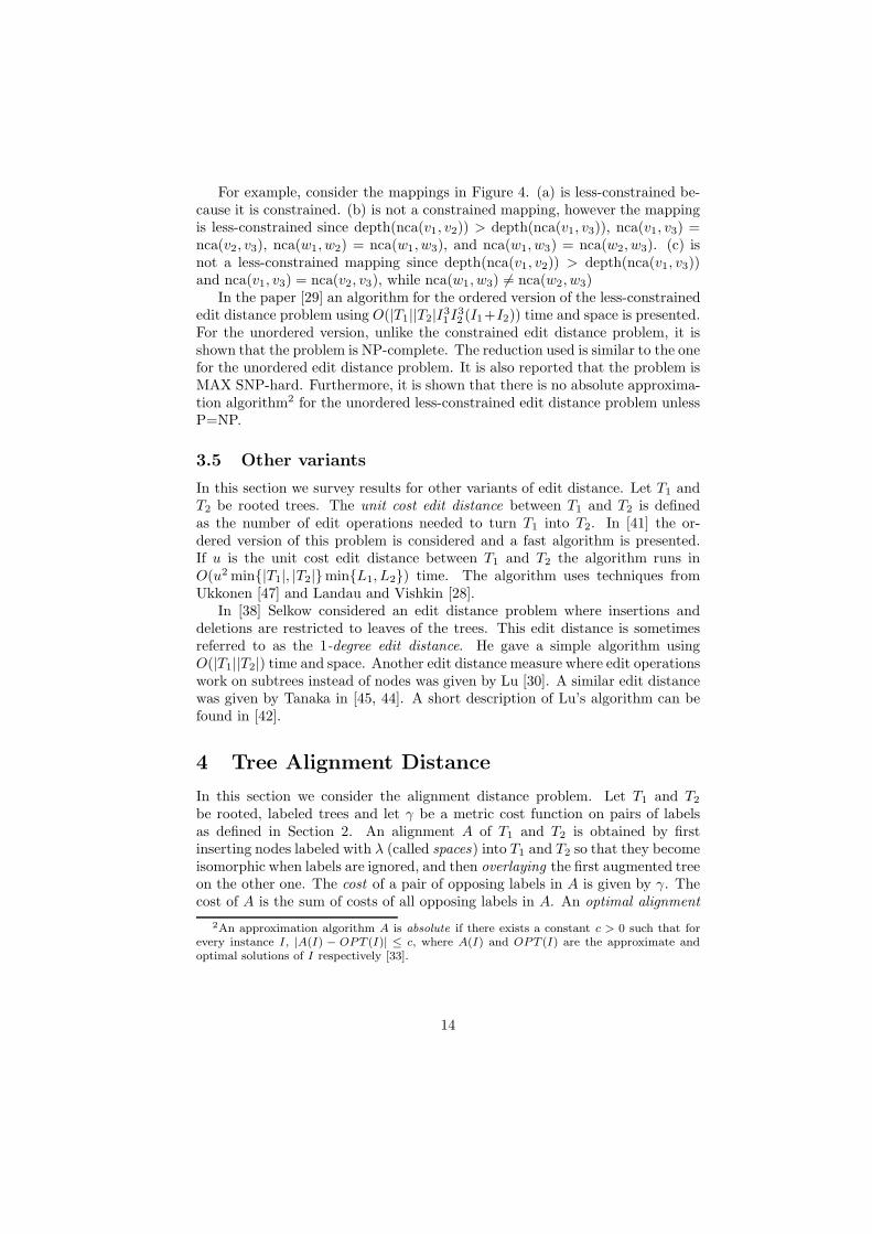
For example, consider the mappings in Figure 4. (a) is less-constrained be-cause it is constrained. (b) is not a constrained mapping, however the mappingis less-constrained since depth(nca(v1, v2)) > depth(nca(v1, v3)), nca(v1, v3) =nca(v2, v3), nca(w1, w2) = nca(w1, w3), and nca(w1, w3) = nca(w2, w3). (c) isnot a less-constrained mapping since depth(nca(v1, v2)) > depth(nca(v1, v3))and nca(v1, v3) = nca(v2, v3), while nca(w1, w3) 6= nca(w2, w3)
In the paper [29] an algorithm for the ordered version of the less-constrainededit distance problem using O(|T1||T2|I
31I3
2 (I1+I2)) time and space is presented.For the unordered version, unlike the constrained edit distance problem, it isshown that the problem is NP-complete. The reduction used is similar to the onefor the unordered edit distance problem. It is also reported that the problem isMAX SNP-hard. Furthermore, it is shown that there is no absolute approxima-tion algorithm2 for the unordered less-constrained edit distance problem unlessP=NP.
3.5 Other variants
In this section we survey results for other variants of edit distance. Let T1 andT2 be rooted trees. The unit cost edit distance between T1 and T2 is definedas the number of edit operations needed to turn T1 into T2. In [41] the or-dered version of this problem is considered and a fast algorithm is presented.If u is the unit cost edit distance between T1 and T2 the algorithm runs inO(u2 min{|T1|, |T2|}min{L1, L2}) time. The algorithm uses techniques fromUkkonen [47] and Landau and Vishkin [28].
In [38] Selkow considered an edit distance problem where insertions anddeletions are restricted to leaves of the trees. This edit distance is sometimesreferred to as the 1-degree edit distance. He gave a simple algorithm usingO(|T1||T2|) time and space. Another edit distance measure where edit operationswork on subtrees instead of nodes was given by Lu [30]. A similar edit distancewas given by Tanaka in [45, 44]. A short description of Lu’s algorithm can befound in [42].
4 Tree Alignment Distance
In this section we consider the alignment distance problem. Let T1 and T2
be rooted, labeled trees and let γ be a metric cost function on pairs of labelsas defined in Section 2. An alignment A of T1 and T2 is obtained by firstinserting nodes labeled with λ (called spaces) into T1 and T2 so that they becomeisomorphic when labels are ignored, and then overlaying the first augmented treeon the other one. The cost of a pair of opposing labels in A is given by γ. Thecost of A is the sum of costs of all opposing labels in A. An optimal alignment
2An approximation algorithm A is absolute if there exists a constant c > 0 such that forevery instance I, |A(I) − OPT (I)| ≤ c, where A(I) and OPT (I) are the approximate andoptimal solutions of I respectively [33].
14

of T1 and T2, is an alignment of T1 and T2 of minimum cost. We denote this costby α(T1, T2). Figure 5 shows an example (from [18]) of an ordered alignment.
a a (a, a)
e d b f (e, λ) (λ, f)
b c c d (b, b) (c, λ) (λ, c) (d, d)
(a) (b) (c)
Figure 5: (a) Tree T1. (b) Tree T2. (c) An alignment of T1 and T2.
The tree alignment distance problem is a special case of the tree editingproblem. In fact, it corresponds to a restricted edit distance where all insertionsmust be performed before any deletions. Hence, δ(T1, T2) ≤ α(T1, T2). Forinstance, assume that all edit operations have cost 1 and consider the examplein Figure 1. The optimal sequence of edit operations is achieved by deleting thenode labeled e and then inserting the node labeled f . Hence, the edit distanceis 2. The optimal alignment, however, is the tree depicted in (c) with a valueof 4. It is a well known fact that edit and alignment distance are equivalent interms of complexity for sequences, see, e.g., Gusfield [14]. However, for treesthis is not true which we will show in the following sections. In Section 4.1 andSection 4.2 we survey the results for the ordered and unordered tree alignmentdistance problem respectively.
4.1 Ordered tree alignment distance
In this section we consider the ordered tree alignment distance problem. Let T1
and T2 be two rooted, ordered and labeled trees. The ordered tree alignmentdistance problem was introduced by Jiang et al. in [18]. The algorithm presentedthere uses O(|T1||T2|(I1 + I2)
2) time and space. Hence, for small degree trees,this algorithm is in general faster than the best known algorithm for the editdistance. We present this algorithm in detail in the next section. Recently, in[17], a new algorithm was proposed designed for similar trees. Specifically, ifthere is an optimal alignment of T1 and T2 using at most s spaces the algorithmcomputes the alignment in time O((|T1|+ |T2|) log(|T1|+ |T2|)(I1 +I2)
4s2). Thisalgorithm works in a way similar to the fast algorithms for comparing similarsequences, see, e.g., Section 3.3.4 in [39]. The main idea is to speedup thealgorithm of Jiang et al. by only considering subtrees of T1 and T2 whose sizesdiffer by at most O(s).
15

4.1.1 Jiang, Wang, and Zhang’s algorithm
In this section we present the algorithm of Jiang et al. [18]. We only show howto compute the alignment distance. The corresponding alignment can easily beconstructed within the same complexity bounds. Let γ be a metric cost functionon the labels. For simplicity, we will refer to nodes instead of labels, that is,we will use (v, w) for nodes v and w to mean (label(v), label(w)). Here, v or w
may be λ. We extend the definition of α to include alignments of forests, thatis, α(F1, F2) denotes the cost of an optimal alignment of forest F1 and F2.
Lemma 7 Let v ∈ V (T1) and w ∈ V (T2) with children v1, . . . , vi and w1, . . . , wj
respectively. Then,
α(θ, θ) = 0
α(T1(v), θ) = α(F1(v), θ) + γ(v, λ)
α(θ, T2(w)) = α(θ, F2(w)) + γ(λ, w)
α(F1(v), θ) =
i∑
k=1
α(T1(vk), θ)
α(θ, F2(w)) =
j∑
k=1
α(θ, T2(wk))
Lemma 8 Let v ∈ V (T1) and w ∈ V (T2) with children v1, . . . , vi and w1, . . . , wj
respectively. Then,
α(T1(v), T2(w)) = min
α(F1(v), F2(w)) + γ(v, w)
α(θ, T2(w)) + min1≤r≤j{α(T1(v), T2(wr)) − α(θ, T2(wr)}
α(T1(v), θ) + min1≤r≤i{α(T1(vr), T2(w)) − α(T1(vr), θ)}
Proof. Consider an optimal alignment A of T1(v) and T2(w). There are fourcases: (1) (v, w) is a label in A, (2) (v, λ) and (k, w) are labels in A for somek ∈ V (T1), (3) (λ, w) and (v, h) are labels in A for some h ∈ V (T2) or (4) (v, λ)and (λ, w) are in A. Case (4) need not be considered since the two nodes canbe deleted and replaced by the single node (v, w) as the new root. The cost ofthe resulting alignment is by the triangle inequality at least as small.
Case 1: The root of A is labeled by (v, w). Hence,
α(T1(v), T2(w)) = α(F1(v), F2(w)) + γ(v, w)
Case 2: The root of A is labeled by (v, λ). Hence, k ∈ V (T1(ws)) for some1 ≤ r ≤ i. It follows that,
α(T1(v), T2(w)) = α(T1(v), θ) + min1≤r≤i
{α(T1(vr), T2(w)) − α(T1(vr), θ)}
Case 3: Symmetric to case 2. �
16

Lemma 9 Let v ∈ V (T1) and w ∈ V (T2) with children v1, . . . , vi and w1, . . . , wj
respectively. For any s, t such that 1 ≤ s ≤ i and 1 ≤ t ≤ j,
α(F1(v1, vs), F2(w1, wt)) = min
α(F1(v1, vs−1), F2(w1, wt−1)) + α(T1(vs), T2(wt))
α(F1(v1, vs−1), F2(w1, wt)) + α(T1(vs), θ)
α(F1(v1, vs), F2(w1, wt−1)) + α(θ, T2(wt))
γ(λ, wt) + min1≤k<s
{α(F1(v1, vk−1), F2(w1, wt−1))
+ α(F1(vk, vs), F2(wk))}γ(vs, λ) + min
1≤k<t{α(F1(v1, vs−1), F2(w1, wk−1))
+ α(F1(vs), F2(wk, wt))}
Proof. Consider an optimal alignment A of F1(v1, vs) and F2(w1, wt). Theroot of the rightmost tree in A is labeled either (vs, wt), (vs, λ) or (λ, wt).
Case 1: The label is (vs, wt). Then the rightmost tree of A must be an optimalalignment of T1(vs) and T2(wt). Hence,
α(F1(v1, vs), F2(w1, wt)) = α(F1(v1, vs−1), F2(w1, wt−1))+α(T1(vs), T2(wt)).
Case 2: The label is (vs, λ). Then T1(vs) is a aligned with a subforest F2(wt−k+1, wt),where 0 ≤ k ≤ t. The following subcases can occur:
2.1 (k = 0). T1(vs) is aligned with F2(wt−k+1, wt) = θ. Hence,
α(F1(v1, vs), F2(w1, wt)) = α(F1(v1, vs−1), F2(w1, wt))+α(T1(vs), θ).
2.2 (k = 1). T1(vs) is aligned with F2(wt−k+1, wt) = T2(wt). Similar tocase 1.
2.3 (k ≥ 2). The most general case. It is easy to see that:
α(F1(v1, vs), F2(w1, wt)) = γ(vs, λ) + min1≤r<t
{α(F1(v1, vs−1), F2(w1, wk−1)))
+ α(F1(vs), F2(wk, wt)).
Case 3: The label is (λ, wt). Symmetric to case 2. �
This recursion can be used to construct a bottom-up dynamic programmingalgorithm. Consider a fixed pair of nodes v and w with children v1, . . . , vi andw1, . . . , wj respectively. We need to compute the values α(F1(vh, vk), F2(w))for all 1 ≤ h ≤ k ≤ i, and α(F1(v), F2(wh, wk)) for all 1 ≤ h ≤ k ≤ j. Thatis, we need to compute the optimal alignment of F1(v) with each subforest ofF2(w) and, on the other hand, compute the optimal alignment of F2(w) witheach subforest of F1(v). For any s and t, 1 ≤ s ≤ i and 1 ≤ t ≤ j, define theset:
As,t = {α(F1(vs, vp), F2(wt, wq)) | s ≤ p ≤ i, t ≤ q ≤ j}
17

To compute the alignments described above we need to compute As,1 and A1,t
for all 1 ≤ s ≤ i and 1 ≤ t ≤ j. Assuming that values for smaller subproblemsare known it is not hard to show that As,t can be computed, using Lemma 9, intime O((i−s) · (j− t) · (i−s+ j− t)) = O(ij(i+ j)). Hence, the time to computeboth of As,1 and A1,t, 1 ≤ s ≤ i and 1 ≤ t ≤ j, is bounded by O(ij(i + j)2). Itfollows that the total time needed for all nodes v and w is bounded by:
∑
v∈V (T1)
∑
w∈V (T2)
O(deg(v) deg(w)(deg(v) + deg(w))2)
≤∑
v∈V (T1)
∑
w∈V (T2)
O(deg(v) deg(w)(deg(T1) + deg(T2))2)
≤ O((I1 + I2)2
∑
v∈V (T1)
∑
w∈V (T2)
deg(v) deg(w))
≤ O(|T1||T2|(I1 + I2)2)
In summary, we have shown the following theorem.
Theorem 3 ([18]) For ordered trees T1 and T2, the tree alignment distanceproblem can be solved in O(|T1||T2|(I1 + I2)
2) time and space.
4.2 Unordered tree alignment distance
The algorithm presented above can be modified to handle the unordered versionof the problem in a straightforward way [18]. If the trees have bounded degreesthe algorithm still runs in O(|T1|T2|) time. This should be seen in contrastto the edit distance problem which is MAX SNP-hard even if the trees havebounded degree. If one tree has arbitrary degree unordered alignment becomesNP-hard [18]. The reduction is, as for the edit distance problem, from the ExactCover by 3-Sets problem [12].
5 Tree Inclusion
In this section we survey the tree inclusion problem. Let T1 and T2 be rooted,labeled trees. We say that T1 is included in T2 if there is a sequence of deleteoperations performed on T2 which makes T2 isomorphic to T1. The tree inclusionproblem is to decide if T1 is included in T2. Figure 6(a) shows an example ofan ordered inclusion. The tree inclusion problem is a special case of the treeedit distance problem: If insertions all have cost 0 and all other operations havecost 1, then T1 can be included in T2 if and only if δ(T1, T2) = 0. Accordingto [7] the tree inclusion problem was initially introduced by Knuth [26][exercise2.3.2-22].
The rest of the section is organized as follows. In Section 5.1 we give somepreliminaries and in Section 5.2 and 5.3 we survey the known results on orderedand unordered tree inclusion respectively.
18

f
f d e
(a) b e a
c
b
f
f d e
(b) b e a
c
b
Figure 6: (a) The tree on the left is included in the tree on the right by deletingthe nodes labeled d, a and c. (b) The embedding corresponding to (a).
5.1 Orderings and embeddings
Let T be a labeled, ordered, and rooted tree. We define an ordering of the nodesof T given by v ≺ v′ iff post(v) < post(v′). Also, v � v′ iff v ≺ v′ or v = v′.Furthermore, we extend this ordering with two special nodes ⊥ and ⊤ such thatfor all nodes v ∈ V (T ), ⊥ ≺ v ≺ ⊤. The left relatives, lr(v), of a node v ∈ V (T )is the set of nodes that are to the left of v and similarly the right relatives, rr(v),are the set of nodes that are to the right of v.
Let T1 and T2 be rooted labeled trees. We define an ordered embedding(f, T1, T2) as an injective function f : V (T1) → V (T2) such that for all nodesv, u ∈ V (T1),
• label(v) = label(f(v)). (label preservation condition)
• v is an ancestor of u iff f(v) is an ancestor of f(u). (ancestor condition)
• v is to the left of u iff f(v) is to the left of f(u). (sibling condition)
Hence, embeddings are special cases of mappings (see Section 3.1). An unorderedembedding is defined as above, but without the sibling condition. An embedding(f, T1, T2) is root preserving if f(root(T1)) = root(T2). Figure 6(b) shows anexample of a root preserving embedding.
5.2 Ordered tree inclusion
Let T1 and T2 be rooted, ordered and labeled trees. The ordered tree inclu-sion problem has been the attention of much research. Kilpelainen and Man-
19

nila [22] (see also [21]) presented the first polynomial time algorithm usingO(|T1||T2|) time and space. Most of the later improvements are refinementsof this algorithm. We present this algorithm in detail in the next section.In [21] a more space efficient version of the above was given using O(|T1|D2)space. In [36] Richter gave an algorithm using O(|ΣT1
||T2| + mT1,T2D2) time,
where ΣT1is the alphabet of the labels of T1 and mT1,T2
is the set matches,defined as the number of pairs (v, w) ∈ T1 × T2 such that label(v) = label(w).Hence, if the number of matches is small the time complexity of this algorithmimproves the (|T1||T2|) algorithm. The space complexity of the algorithm isO(|ΣT1
||T2| + mT1,T2). In [7] a more complex algorithm was presented using
O(L1|T2|) time and O(L1 min{D2, L2}) space. In [3] an efficient average casealgorithm was given.
5.2.1 Kilpelainen and Mannila’s algorithm
In this section we present the algorithm of Kilpelainen and Mannila [22] for theordered tree inclusion problem. Let T1 and T2 be ordered labeled trees. DefineR(T1, T2) as the set of root-preserving embeddings of T1 into T2. We defineρ(v, w), where v ∈ V (T1) and w ∈ V (T2):
ρ(v, w) = min≺
({w′ ∈ rr(w) | ∃f ∈ R(T1(v), T2(w′))} ∪ {⊤})
Hence, ρ(v, w) is the closest right relative of w which has a root-preservingembedding of T1(v). Furthermore, if no such embedding exists ρ(v, w) is ⊤.It is easy to see that, by definition, T1 can be included in T2 if and only ifρ(v,⊥) 6= ⊤. The following lemma shows how to search for root preservingembeddings.
Lemma 10 Let v be a node in T1 with children v1, . . . , vi. For a node w inT2, define a sequence p1, . . . , pi by setting p1 = ρ(v1, max≺ lr(w)) and pk =ρ(vk, pk−1), for 2 ≤ k ≤ i. There is a root preserving embedding f of T1(v) inT2(v) if and only if label(v) = label(w) and pi ∈ T2(w), for all 1 ≤ k ≤ i.
Proof. If there is a root preserving embedding between T1(v) and T2(w) it isstraightforward to check that there is a sequence pi, 1 ≤ i ≤ k such that theconditions are satisfied. Conversely, assume that pk ∈ T2(w) for all 1 ≤ k ≤ i
and label(v) = label(w). We construct a root-preserving embedding f of T1(v)into T2(w) as follows. Let f(v) = w. By definition of ρ there must be a rootpreserving embedding fk, 1 ≤ k ≤ i, of T1(vk) in T2(pk). For a node u in T1(vk),1 ≤ k ≤ i, we set f(u) = fk(u). Since pk ∈ rr(pk−1), 2 ≤ k ≤ i, and pk ∈ T2(w)for all k, 1 ≤ k ≤ i, it follows that f is indeed a root-preserving embedding. �
Using dynamic programming it is now straightforward to compute ρ(v, w)for all v ∈ V (T1) and w ∈ V (T2). For a fixed node v we traverse T2 in reversepostorder. At each node w ∈ V (T2) we check if there is a root preservingembedding of T1(v) in T2(w). If so we set ρ(v, q) = w, for all q ∈ lr(w) suchthat x � q, where x is the next root-preserving embedding of T1(v) in T2(w).
20

For a pair of nodes v ∈ V (T1) and w ∈ V (T2) we test for a root-preservingembedding using Lemma 10. Assuming that values for smaller subproblems hasbeen computed, the time used is O(deg(v)). Hence, the contribution to the totaltime for the node w is
∑
v∈V (T1) O(deg(v)) = O(|T1|). It follows that the time
complexity of the algorithm is bounded by O(|T1||T2|). Clearly, only O(|T1||T2|)space is needed to store ρ. Hence, we have the following theorem,
Theorem 4 ([22]) For any pair of rooted, labeled, and ordered trees T1 andT2, the tree inclusion problem can be solved in O(|T1||T2|) time and space.
5.3 Unordered tree inclusion
In [22] it is shown that the unordered tree inclusion problem is NP-complete.The reduction used is from the Satisfiability problem [12]. Independently, Ma-tousek and Thomas [32] gave another proof of NP-completeness.
An algorithm for the unordered tree inclusion problem is presented in [22]using O(|T1|I12
2I1 |T2|) time. Hence, if I1 is constant the algorithm runs inO(|T1||T2|) time and if I1 = log |T2| the algorithm runs in O(|T1| log |T2||T2|
3).
6 Conclusion
We have surveyed the tree edit distance, alignment distance, and inclusion prob-lems. Furthermore, we have presented, in our opinion, the central algorithmsfor each of the problems. There are several open problems, which may be thetopic of further research. We conclude this paper with a short list proposingsome directions.
• For the unordered versions of the above problems some are NP-completewhile others are not. Characterizing exactly which types of mappingsthat gives NP-complete problems for unordered versions would certainlyimprove the understanding of all of the above problems.
• The currently best worst case upper bound on the ordered tree edit dis-tance problem is the algorithm of [25] using O(|T1|
2|T2| log |T2|). Con-versely, the quadratic lower bound for the longest common subsequenceproblem [1] problem is the best general lower bound for the ordered treeedit distance problem. Hence, a large gap in complexity exists which needsto be closed.
• Several meaningful edit operations other than the above may be considereddepending on the particular application. Each set of operations yield anew edit distance problem for which we can determine the complexity.Some extensions of the tree edit distance problem have been considered[6, 5, 24].
21

Acknowledgements
Thanks to Inge Li Gørtz and Anna Ostlin for proof reading and helpful discus-sions.
References
[1] A. V. Aho, J. D. Ullman, and D. S. Hirschberg. Bounds on the complexityof the longest common subsequence problem. Journal of the ACM (JACM),1(23):1–12, January 1976.
[2] T. Akutsu and M. M. Halldorsson. On the approximation of largest com-mon point sets and largest common subtrees. In Proceedings of the 5th An-nual International Symposium on Algorithms and Computation, in LectureNotes in Computer Science (LNCS), volume 834, pages 405–413. Springer,1994.
[3] L. Alonso and R. Schott. On the tree inclusion problem. In Proceedings ofMathematical Foundations of Computer Science, pages 211–221, 1993.
[4] A. Arora, C. Lund, R. Motwani, M. Sudan, and M. Szegedy. Proof verifi-cation and hardness of approximation problems. In Proceedings of the 33rdIEEE Symposium on the Foundations of Computer Science (FOCS), pages14–23, 1992.
[5] S. Chawathe and H. Garcia-Molina. Meaningful change detection in struc-tured data. In Proceedings of the ACM SIGMOD International Conferenceon Management of Data, pages 26–37, Tuscon, Arizona, 1997.
[6] S. S. Chawathe, A. Rajaraman, H. Garcia-Molina, and J. Widom. Changedetection in hierarchically structured information. In Proceedings of theACM SIGMOD International Conference on Management of Data, pages493–504, Montreal, Quebec, June 1996.
[7] Weimin Chen. More efficient algorithm for ordered tree inclusion. Journalof Algorithms, 26:370–385, 1998.
[8] Weimin Chen. New algorithm for ordered tree-to-tree correction problem.Journal of Algorithms, 40:135–158, 2001.
[9] Thomas H. Cormen, Charles E. Leiserson, Ronald L. Rivest, and CliffordStein. Introduction to Algorithms, second edition. MIT Press, 2001.
[10] Moshe Dubiner, Zvi Galil, and Edith Magen. Faster tree pattern match-ing. In Proceedings of the 31st IEEE Symposium on the Foundations ofComputer Science (FOCS), pages 145–150, 1990.
[11] Martin Farach and Mikkel Thorup. Fast comparison of evolutionary trees.In Proceedings of the 5th Annual ACM-SIAM Symposium on Discrete Al-gorithms, pages 481–488, 1994.
22
[12] Michael J. Garey and David S. Johnson. Computers and Intractability: AGuide to the Theory of NP-completeness. Freeman, 1979.
[13] Arvind Gupta and Naomi Nishimura. Finding largest subtrees and smallestsupertrees. Algorithmica, 21:183–210, 1998.
[14] D. Gusfield. Algorithms on Strings, Trees, and Sequences. CambridgeUniversity Press, 1997.
[15] D. Harel and R. E. Tarjan. Fast algorithms for finding nearest commonancestors. SIAM Journal of Computing, 13(2):338–355, 1984.
[16] Christoph M. Hoffmann and Michael J. O’Donnell. Pattern matchingin trees. Journal of the Association for Computing Machinery (JACM),29(1):68–95, 1982.
[17] Jesper Jansson and Andrzej Lingas. A fast algorithm for optimal align-ment between similar ordered trees. In Proceedings of the 12th AnnualSymposium on Combinatorial Pattern Matching (CPM), in Lecture notesof Computer Science (LNCS), volume 2089. Springer, 2001.
[18] Tao Jiang, Lusheng Wang, and Kaizhong Zhang. Alignment of trees – analternative to tree edit. Theoretical Computer Science (TCS), 143, 1995.
[19] Dmitry Keselman and Amihood Amir. Maximum agreement subtree in aset of evolutionary trees – metrics and efficient algorithms. In Proceedings ofthe 35th Annual Symposium on Foundations of Computer Science (FOCS),pages 758–769, 1994.
[20] S. Khanna, R. Motwani, and F. F. Yao. Approximation algorithms for thelargest common subtree problem. Technical report, Stanford University,1995.
[21] Pekka Kilpelainen. Tree Matching Problems with Applications to Struc-tured Text Databases. PhD thesis, University of Helsinki, Department ofComputer Science, November 1992.
[22] Pekka Kilpelainen and Heikki Mannila. Ordered and unordered tree inclu-sion. SIAM Journal of Computing, 24:340–356, 1995.
[23] Philip Klein, 2002. Personal communication.
[24] Philip Klein, Srikanta Tirthapura, Daniel Sharvit, and Ben Kimia. A tree-edit-distance algorithm for comparing simple, closed shapes. In Proceed-ings of the 11th Annual ACM-SIAM Symposium on Discrete Algorithms(SODA), pages 696–704, 2000.
[25] P.N. Klein. Computing the edit-distance between unrooted ordered trees.In Proceedings of the 6th annual European Symposium on Algorithms (ESA)1998., pages 91–102. Springer-Verlag, 1998.
23

[26] Donald Erwin Knuth. The Art of Computer Programming, Volume 1. Ad-dison Wesley, 1969.
[27] S. Rao Kosaraju. Efficient tree pattern matching. In Proceedings of the30th IEEE Symposium on the Foundations of Computer Science (FOCS),pages 178–183, 1989.
[28] G. M. Landau and U. Vishkin. Fast parallel and serial approximate stringmatching. Journal of Algorithms, 10:157–169, 1989.
[29] Chin Lung Lu, Zheng-Yao Su, and Chuan Yi Tang. A new measure of editdistance between labeled trees. In Proceedings of the 7th Annual Interna-tional Conference on Computing and Combinatorics (COCOON), volume2108 of Lecture Notes in Computer Science (LNCS). Springer, 2001.
[30] S. Y. Lu. A tree-to-tree distance and its application to cluster analysis.IEEE Transactions on Pattern Analysis and Machine Intelligence (PAMI),1:219–224, 1979.
[31] S. Y. Lu. A tree-matching algorithm based on node splitting and merging.IEEE Transactions on Pattern Analysis and Machine Intelligence (PAMI),6(2):249–256, 1984.
[32] Jiri Matousek and R. Thomas. On the complexity of finding iso- and othermorphisms for partial k-trees. Discrete Mathematics, 108:343–364, 1992.
[33] Rajeev Motwani. Lecture notes on approximation algorithms volume 1.Technical Report STAN-CS-92-1435, Stanford University, Department ofComputer Science, 1992.
[34] Naomi Nishimura, Prabhakar Ragde, and Dimitrios M. Thilikos. Findingsmallest supertrees under minor containment. International Journal ofFoundations of Computer Science, 11(3):445–465, 2000.
[35] R. Ramesh and I.V. Ramakrishnan. Nonlinear pattern matching in trees.Journal of the Association for Computing Machinery (JACM), 39(2):295–316, 1992.
[36] Thorsten Richter. A new algorithm for the ordered tree inclusion problem.In Proceedings of the 8th Annual Symposium on Combinatorial PatternMatching (CPM), in Lecture Notes of Computer Science (LNCS), volume1264, pages 150–166. Springer, 1997.
[37] Thorsten Richter. A new measure of the distance between ordered trees andits applications, technical report 85166-cs. Technical report, Departmentof Computer Science, University of Bonn, 1997.
[38] Stanley M. Selkow. The tree-to-tree editing problem. Information Process-ing Letters, 6(6):184–186, 1977.
24

[39] J. Setubal and J. Meidanis. Introduction to Computational Biology. PWSPublishing Company, 1997.
[40] Dennis Shasha, Jason Tsong-Li Wang, Huiyuan Shan, and Kaizhong Zhang.Atreegrep: Approximate searching in unordered trees. In Proceedings ofthe 14th International Conference on Scientific and Statistical DatabaseManagement, pages 89–98, 2002.
[41] Dennis Shasha and Kaizhong Zhang. Fast algorithms for the unit costediting distance between trees. Journal of Algorithms, 11:581–621, 1990.
[42] Dennis Shasha and Kaizhong Zhang. Approximate tree pattern matching.In Pattern Matching in String, Trees and Arrays, pages 341–371. OxfordUniversity, 1997.
[43] Kuo-Chung Tai. The tree-to-tree correction problem. Journal of the Asso-ciation for Computing Machinery (JACM), 26:422–433, 1979.
[44] Eiichi Tanaka. A note on a tree-to-tree editing problem. InternationalJournal of Pattern Recognition and Artificial Intelligence, 9(1):167–172,1995.
[45] Eiichi Tanaka and Keiko Tanaka. The tree-to-tree editing problem. Interna-tional Journal of Pattern Recognition and Artificial Intelligence, 2(2):221–240, 1988.
[46] Srikanta Tirthapura, Daniel Sharvit, Philip Klein, and Benjamin B. Kimia.Indexing based on edit-distance matching of shape graphs. In Proceedingof SPIE International Symposium on Voice, Video and Data Communica-tions, pages 91–102, 1998.
[47] Esko Ukkonen. Finding approximate patterns in strings. Journal of Algo-rithms, 6:132–137, 1985.
[48] Robert A. Wagner and Michael J. Fischer. The string-to-string correctionproblem. Journal of the ACM (JACM), 21:168–173, 1974.
[49] Jason Tsong-Li Wang, Kaizhong Zhang, Karpjoo Jeong, and DennisShasha. A system for approximate tree matching. IEEE Transactionson Knowledge and Data Engineering, 6(4):559–571, 1994.
[50] Kaizhong Zhang. The Editing Distance Between Trees: Algorithms andApplications. PhD thesis, Courant Institute, Departement of ComputerScience, 1989.
[51] Kaizhong Zhang. Algorithms for the constrained editing problem betweenordered labeled trees and related problems. Pattern Recognition, 28:463–474, 1995.
[52] Kaizhong Zhang. A constrained edit distance between unordered labeledtrees. Algorithmica, 15(3):205–22, 1996.
25

[53] Kaizhong Zhang. Efficient parallel algorithms for tree editing problems. InProceedings of the 7th Annual Symposium Combinatorial Pattern Matching(CPM), in Lecture Notes in Computer Science 1075, pages 361–372, 1996.
[54] Kaizhong Zhang and Tao Jiang. Some MAX SNP-hard results concerningunordered labeled trees. Information Processing Letters, 49:249–254, 1994.
[55] Kaizhong Zhang and Dennis Shasha. Simple fast algorithms for the editingdistance between trees and related problems. SIAM Journal of Computing,18:1245–1262, 1989.
[56] Kaizhong Zhang, Dennis Shasha, and Jason T. L. Wang. Approximatetree matching in the presence of variable length don’t cares. Journal ofAlgorithms, 16(1):33–66, 1994.
[57] Kaizhong Zhang, Rick Statman, and Dennis Shasha. On the editing dis-tance between unordered labeled trees. Technical Report 289, The Univer-sity of Western Ontario, Departement of Computer Science, 1991.
[58] Kaizhong Zhang, Rick Statman, and Dennis Shasha. On the editing dis-tance between unordered labeled trees. Information Processing Letters,42:133–139, 1992.
26

Tree edit distancevariant type time space referencegeneral O O(|T1||T2|D
21D
22) O(|T1||T2|D
21D
22) [43]
general O O(|T1||T2|min(L1, D1)min(L2, D2)) O(|T1||T2|) [55]general O O(|T1|
2|T2| log |T2|) O(|T1||T2|) [25]general O O(|T1||T2| + L2
1|T2| + L2.51 L2) O((|T1| + L2
1)min(L2, D2) + |T2|) [8]general U MAX SNP-hard [54]
constrained O O(|T1||T2|) O(|T1||T2|) [51]constrained O O(|T1||T2|I1I2) O(|T1||D2I2) [37]constrained U O(|T1||T2|(I1 + I2) log(I1 + I2)) O(|T1||T2|) [52]
less-constrained O O(|T1||T2|I31I3
2 (I1 + I2)) O(|T1||T2|I31I3
2 (I1 + I2)) [29]less-constrained U MAX SNP-hard [29]
unit-cost O O(u2 min(|T1|, |T2|)min(L1, L2)) O(|T1||T2|) [41]1-degree O O(|T1||T2|) O(|T1||T2|) [38]
Tree alignment distancegeneral O O(|T1||T2|(I1 + I2)
2) O(|T1||T2|(I1 + I2)2) [18]
general U MAX SNP-hard [18]similar O O((|T1| + |T2|) log(|T1| + |T2|)(I1 + I2)
4s2) O((|T1| + |T2|) log(|T1| + |T2|)(I1 + I2)4s2) [17]
Tree inclusiongeneral O O(|T1||T2|) O(|T1|min(D2L2)) [21]general O O(|ΣT1
||T2| + mT1,T2D2) O(|ΣT1
||T2| + mT1,T2) [36]
general O O(L1|T2|) O(L1 min(D2L2)) [7]general U NP-hard [22, 32]
Table 1: Results for the tree edit distance, alignment distance, and inclusion problem listed according to variant. Di, Li, andIi denotes the depth, the number of leaves, and the maximum degree respectively of Ti, i = 1, 2. The type is either O forordered or U for unordered. The value u is the unit cost edit distance between T1 and T2 and the value s is the number ofspaces in the optimal alignment of T1 and T2. The value ΣT1
is set of labels used in T1 and mT1,T2is the number of pairs of
nodes in T1 and T2 which have the same label.
27