A Survey on Understanding, Visualizations, andExplanation of Deep Neural Networks

Atefeh Shahroudnejad†

† Concordia Institute for Information Systems Engineering, Concordia University, Montreal, Canada

Abstract—Recent advancements in machine learning and sig-nal processing domains have resulted in an extensive surgeof interest in Deep Neural Networks (DNNs) due to theirunprecedented performance and high accuracy for differentand challenging problems of significant engineering importance.However, when such deep learning architectures are utilized formaking critical decisions such as the ones that involve humanlives (e.g., in control systems and medical applications), it is ofparamount importance to understand, trust, and in one word“explain” the argument behind deep models’ decisions. In manyapplications, artificial neural networks (including DNNs) areconsidered as black-box systems, which do not provide sufficientclue on their internal processing actions. Although some recentefforts have been initiated to explain the behaviors and decisionsof deep networks, explainable artificial intelligence (XAI) domain,which aims at reasoning about the behavior and decisions ofDNNs, is still in its infancy. The aim of this paper is to providea comprehensive overview on Understanding, Visualization, andExplanation of the internal and overall behavior of DNNs.

Index Terms: Interpretability, Opening the black-box,Understanding and Visualization of Deep Neural Net-works, Convolutional Neural Network (CNN), RecurrentNeural Network (RNN), Explainable Artificial Intelligence(XAI), Explainability by Design

I. INTRODUCTION

Nowadays, advanced machine learning techniques [1]–[5]have strongly influenced all aspects of our lives by takingover human roles in different complicated tasks. As such,critical decisions are being made based on machine learn-ing models’ predictions with limited human intervention orsupervision. Among such machine learning techniques, deepneural networks (DNNs) [5], such as convolutional neural net-works (CNNs) [6] and recurrent neural networks (RNNs) [2][7], have shown unprecedented performance specially in im-age/video processing and computer vision tasks. However,such deep architectures are extremely complex, full of non-linearities, and also not fully transparent; therefore, it is vitalto understand what operations or input information lead to aspecific decision before deploying such complex models inmission-critical applications. Consequently, it is undeniablynecessary to build the trust of a deep model by validatingits predictions, and be certain that it performs as expected and

reliably on unseen or unfamiliar real-world data. In particular,in critical domains such as biomedical applications [8] andautonomous vehicles (self-driving cars) [9], a single incorrectdecision cannot be tolerated as it could possibly lead tocatastrophic consequences and even threat human lives. Toguarantee the reliability of a machine learning model, it isimperative to understand, analyze, visualize, and in one wordexplain the rational reasons behind its decisions, which is thefocus of this article. Despite its importance, explainabilityof DNNs is still in its infancy and a long road is ahead toopen the ”black-box” of DNNs. Explainability can be fulfilledvisually (focus of this work), text based or example based [10].Generally speaking, the main goal of an explainable DNN isto find answers to questions of like: What is happening insidea DNN? What does each layer of a deep architecture do? Whatfeatures is a DNN looking for? Why should we trust decisionsmade by a neural network? Having appropriate answers tothese questions through development of explainable modelsresults in the following advantages [11]: (i) Verification of themodel; (ii) Improving a model by understanding its failurepoints; (iii) Extracting new insights and hidden laws of themodel, and; (iv) Identifying modules responsible for incorrectdecisions. To achieve these goals, we focus on the followingaspects:• Visualizing and Understanding DNNs: We start by

visualizing features in pre-trained networks to understandthe learned kernels (in CNNs) and data structures (inRNNs). We analyze the behavior of DNNs from this pointof view and call it Structural Analysis.

• Explaining DNNs: We specifically describe the overalland internal behaviors of DNNs in the explainability con-cept. Overall behavior (functional analysis) is based oninput-output relations, while, internal behavior (decisionanalysis) tries to dive into mathematical derivatives todescribe the decision.

• Explainability by Design: We look into bringing explain-ability properties into the network design instead of tryingto explain a pre-trained network with fixed structure.In other words, we explore DNN architectures that areinherently explainable and discuss how explainability canbe achieved by design in general.

arX

iv:2

102.

0179

2v1

[cs

.LG

] 2

Feb

202

1

2

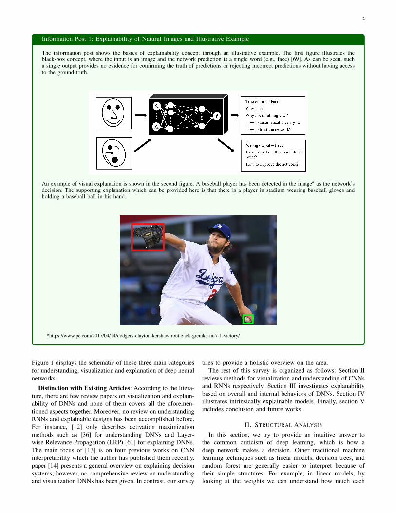
Information Post 1: Explainability of Natural Images and Illustrative Example

The information post shows the basics of explainability concept through an illustrative example. The first figure illustrates theblack-box concept, where the input is an image and the network prediction is a single word (e.g., face) [69]. As can be seen, sucha single output provides no evidence for confirming the truth of predictions or rejecting incorrect predictions without having accessto the ground-truth.

An example of visual explanation is shown in the second figure. A baseball player has been detected in the imagea as the network’sdecision. The supporting explanation which can be provided here is that there is a player in stadium wearing baseball gloves andholding a baseball ball in his hand.

ahttps://www.pe.com/2017/04/14/dodgers-clayton-kershaw-rout-zack-greinke-in-7-1-victory/

Figure 1 displays the schematic of these three main categoriesfor understanding, visualization and explanation of deep neuralnetworks.

Distinction with Existing Articles: According to the litera-ture, there are few review papers on visualization and explain-ability of DNNs and none of them covers all the aforemen-tioned aspects together. Moreover, no review on understandingRNNs and explainable designs has been accomplished before.For instance, [12] only describes activation maximizationmethods such as [36] for understanding DNNs and Layer-wise Relevance Propagation (LRP) [61] for explaining DNNs.The main focus of [13] is on four previous works on CNNinterpretability which the author has published them recently.paper [14] presents a general overview on explaining decisionsystems; however, no comprehensive review on understandingand visualization DNNs has been given. In contrast, our survey

tries to provide a holistic overview on the area.The rest of this survey is organized as follows: Section II

reviews methods for visualization and understanding of CNNsand RNNs respectively. Section III investigates explanabilitybased on overall and internal behaviors of DNNs. Section IVillustrates intrinsically explainable models. Finally, section Vincludes conclusion and future works.

II. STRUCTURAL ANALYSIS

In this section, we try to provide an intuitive answer tothe common criticism of deep learning, which is how adeep network makes a decision. Other traditional machinelearning techniques such as linear models, decision trees, andrandom forest are generally easier to interpret because oftheir simple structures. For example, in linear models, bylooking at the weights we can understand how much each

3

Underestanding,Visualization and

Explanation of DNNs

Structural Analysis

CNNs RNNs

BehaviouralAnalysis

FunctionalAnalysis

DecisionAnalysis

Explainabilityby Design

First LayerFeaturesIntermediateLayers Features

Last LayerFeatures

CapsNet

CNN/FF

semanticalobject-part filters

Fig. 1: Overall categorization for understanding, visualization an explanation of deep neural networks

input feature effects the decision. Hence, several methods havebeen proposed to evidence the meaningful conduct of deepnetworks. In this regard, we investigate CNNs and RNNsas two fundamental categories of DNNs and analyze howinformation is restructured and represented during the learningprocess by these networks.

A. Understanding Convolutional Neural Networks

CNNs contribute significantly to the recent success andinterest of DNNs. The most widely used CNN architec-tures include AlexNet [6], VGGNet [15], ResNet [16],GoogleNet [18] and DenseNet [19], among others. Each con-volutional layer in a CNN (Fig. 2) includes several filters suchthat each of these filters will be highly activated by a patternpresent in the training set (e.g., one kernel might be lookingfor curves), which in turn is considered as a ”template”. Assuch, interpreting the chain of these learned filters based ondifferent inputs can explain complex decisions maid by CNNsand how the results are achieved. To visualize and understandthe learned features of a CNN, we focus on three distinct levelsas specified below.

Fig. 2: A regular CNN architecture including convolutional layers (”Conv”),pooling layers (”Pool”), and fully-connected layers (”FC”).

A.1. First Layer Features: Within the first layer, consideringthat the pixel space is available, filters can be visualized byprojection to this space [6]. The weights of convolutionalfilters in the first layer of a pre-trained model, indicates whattype of low-level features they are looking for, e.g., orientededges with different positions and angels or various opposingcolors. In the next layer, these features are combined togetheras higher level features, e.g., corner and curves. This processcontinues and in each subsequent layer more complete featureswill be extracted.

In the first convolutional layer, raw pixels of an input imageare fed to the network. Convolutional filters in this layer slideover the input image to obtain inner products between theirweights and each image patch which provides the first layerfeature maps. Since it is a direct inner product between thefilters’ weights and pixels of input image in the first layer, wecan somehow understand what these filters are looking for byvisualizing the learned filters’ weights. The intuition behindit comes from template matching. The inner product will bemaximized when both vectors are the same. For instance, thereare 96 filters of 11 × 11 × 3 dimension in the first layer ofAlexNet. Each of these 11 × 11 × 3 filters can be visualizedas a three-channels (RGB) 11× 11 small image [6] (Fig. 3).

As shown in Fig. 3, there are opposing colors (like blueand orange, pink and green) and oriented edges with differentangels and positions. This is similar to human visual systemwhich detects basic features like oriented edges in its earlylayers [27]. Independent of the architecture and the type oftraining data, the first layer filters always contain opposingcolors (if inputs are color images) and oriented edges.

A.2. Intermediate Layers Features:Visualizing features associated with the higher layers of

a DNN cannot be accomplished as easy as the first layerdiscussed above, because projection to pixel space is notstraightforward (higher layers are connected to their previouslayer output instead of connecting directly to the input image).

4

Fig. 3: 96 first layer convolutional filters (with size 11 × 11 × 3) of pre-trained Alexnet model [6].

Therefore, if the same visualization procedure is conducted forthe weights of the intermediate convolutional layers (simillarin nature to the approach used for the first layer), we cansee which pattern activate these layers maximally; but thevisualized patterns are not quite understandable. Since we donot know what previous layer outputs look like in terms ofimage pixels, we cannot interpret what these filters are lookingfor. For instance, Fig. 4 indicates this weight visualization forthe second convolutional layer.

Hence, other alternative approaches are required to discoveractivities of higher layers. This sub-section investigates meth-ods to understand CNNs based on filters in the intermediatelayers and presents their incorporation in a few interestingapplications, i.e., feature inversion, style transfer and GoogleDeepDream1.

Maximizing filters’ activation maps or class scores throughback-propagating them to the pixel space is called gradient-based approach. This common visualization approach helps tofind out how much a variation in an input image effects ona unit score [36]. Also, patterns or patches in input images,which activate a specific unit, will be discovered.

In the following, we demonstrate the gradient-based meth-ods in intermediate layers.

Reference [29] visualizes intermediate features by exploringwhat types of input image patches cause different neurons’maximal activations. Generally, each image patch stimulatesa specific neuron. The algorithm is running many imagesthrough the pre-trained network and recording feature valuesfor a particular neuron in a particular layer (e.g. Conv5). Thenimage patches in dataset corresponding to the parts of that neu-ron which has been maximally activated, are visualized. Here,to detect most responsible pixels for higher activation of a neu-

1https://ai.googleblog.com/2015/06/inceptionism-going-deeper-into-neural.html

ron through deconvolution process, the paper proposes GuidedBack-propagation instead of regular back-propagation to havemuch cleaner result images. In Guided Back-propagation sinceonly positive gradients are back-propagated through ReLUs,only positive influences are tracked throughout the network.The intuition behind this projection down to pixel space isobtaining saliency map for that neuron (same as saliencymap for a class score described in section III-A) which isaccomplished by computing the gradient of each neuron valuewith respect to the input image pixels.

However, for more understanding it is necessary to knowwhat type of input in general maximizes the score of anintermediate neuron (or a class score in case of section III-A)and causes this neuron to be maximally activated. For thispurpose, in a pre-trained network with fix weights, gradientascent is applied iteratively on pixels of a zeros-(or uniformly)initialized image which is called synthesized image and it isupdated accordingly. Here, a regularization term is needed toprevent pixels of the generated image from overfitting to somespecific features of the network. The generated image shouldmaximally activate a neuron value (or a class score) whileappearing to be a natural image. Hence, it should have thestatistics of natural images and a regularization term (Rθ(X))shall force it to look almost natural. A common regularizer isthe L2 norm of synthesized image (‖X‖2), which penalizesextremely large pixel values. But through this regularization,the quality of generated results is not enough and therefore itneeds to be improved by improving regularization term insteadof using just L2 one.

In this regard, paper [28] uses two other regularizers inaddition to L2 norm as natural image priors which are: theGaussian blur to penalize high frequency information; settingpixels with small values or low gradients to zero duringthe optimization procedure (Eq. (1)). Using these regularizersmakes generated results look more impressive and much clearto see.

X∗ = argmaxX

(fi(X)−Rθ(X)) (1)

[28] generally proposes an interactive deep visualization andinterpreting toolbox whose input can be an image or a video.The toolbox displays neurons’ activations on a selected layerof a pre-trained network and it gives the intuition of whatthat layer’s neurons are doing. For example, units in thefirst layer response strongly to sharp edges. On the otherhand, in higher layers (e.g., Conv5) they response to moreabstract concepts (e.g. cat’s face in cat image). The toolboxalso shows synthesized images to produce high activation viaregularized gradient ascent as mentioned before. It means thatthe neuron fires in response to a specific concept. By feedingall training set images and selecting top ones that activatethe particular neuron most and also computing pixels whichare most responsible for the neuron’s high activation throughbackward deconvolution process, we can concretely analyzethat neuron.

In references [33], [34], the weights of the output layer (e.g.,class scores) are back-propagated to the last convolutional

1https://cs.stanford.edu/people/karpathy/convnetjs/demo/cifar10.html

5

Fig. 4: Visualizing filters’ weights of second convolutional layer same as the first layer visualization. Here, there are 20 filters with size 5× 5× 16. Thisvisualization has been taken from ConvNetJS CIFAR-10 demo1.

layer to determine the importance of each activation map inthe decision. Moreover, GradCAM [33] and Guided Back-propagation [29] can be combined together through element-wise product to result more specific feature importance [33].

Another approach to improve visualization is consideringextra features. In this regard, paper [37] tries to explicitlyconsider multiple facets (feature types) of a neuron in theoptimization procedure rather than assuming only one featuretype. ”Multiple facets” refers to different types of imagesin the dataset where all of them are in the same class andconvey same concept (e.g. different colors of an object).To visualize a neuron’s multiple facets, the algorithm firstuses k-means to cluster all different images which highlyactivate the neuron. Each cluster is considered as a differentfacet and the mean of its images is used to initialize asynthesized image for the facet. Then, activation maximizationprocedure of the neuron is applied to all facets’ synthesizedimages. Paper [38] proposes a deep image generator network(DGN) as a learned natural image prior for synthesized imagein activation maximization framework. The generator is thegenerator part of GAN, which is trained to invert extractedfeature representation by the encoder such that the synthesizedimage has features close to real images and the discriminatorcan not distinguish it from real ones. The final objectiveis optimizing latent space representation (instead of pixelspace) to generate a synthesized image which maximizes theactivation of determined neuron. By adding such additionalpriors toward modeling natural images, we can generate veryrealistic images at the end which indicate what the neuronsare looking for.

In the following, we briefly refer to the most popularapplications of understanding intermediate filters.

Applications: The idea of synthesizing images using gradi-ent ascent is quite powerful and it can be used for generatingadversarial examples to fool the network. By choosing anarbitrary image and an arbitrary class, the algorithm startsmodifying the image to maximize the selected class scoreand repeats this process until the network is fooled. Theresults are much surprising because they look same as originalimages but they are classified as selected classes. Google has

also proposed another application named DeepDream, whichcreates dreamy hallucinogenic images. It again indicates whatfeatures the network are looking for. DeepDream tries toamplify some existing features which have been detected bythe network in an input image through maximizing neuronactivations in a layer. After running an input image throughthe pre-trained network up to the chosen layer, the gradientof that layer (which is equal to its activation (Eq. (2))) iscomputed with respect to input image pixels and the inputimage is updated iteratively to maximize this layer activation.when we select lower layers, many edges and swirls pop upin the image. On the other hand by selecting higher layers,some meaningful objects appear in the image.

I∗ = argmaxI

∑i

fi(I)2 (2)

Feature inversion concept indicates what types of imageelements are captured at different layers of the network. Infeature inversion an image runs through the pre-trained net-work and its feature values are recorded. After reconstructingthat image from the feature representation of different layers,regarding what reconstructed images look like, they give somesense about how much information have been captured in thesefeature vectors [31]. For instance, if the image is reconstructedbased on first layers’ features (e.g. ReLU2 in VGG-16), wecan see the image is well reconstructed which means thatless information is thrown away at these layers. in contrast,in deeper layers although the general spatial structure of theimage is preserved, a lot of low level details such as exactpixel values, colors and texture are lost which means that inhigher layers the network is throwing away these kind of lowlevel information and instead it focuses on keeping aroundmore semantic information. It synthesizes a new image (X)by matching its features (Φ(X)) back to that recorded features(Φ0) which are computed before for that layer. It minimizesthe distance between them using gradient-ascent and total-variation regulariser (Eq. (3)).

X∗ = argminX∈<H×W×C

‖Φ(X)− Φ0‖2 + λRV β (X), (3)

6

where the result image (X∗) has the most similar features

to the recorded ones. λ is the regularizer coefficient, andtotal variation regularizer (RV β ) is another natural image priorwhich penalizes differences between adjacent pixels verticallyand horizontally, which makes the generated image smoother.However, this natural image objective is hardly achieved inpractice. Therefore, the authors improved their method usingnatural pre-images and more appropriate regularizers [32].

Feature reconstruction loss is also used in single imagesuper-resolution problem [22]. It transfers semantic knowledgein this way and therefore it can more precisely reconstructsfine details and tiny edges rather than previous methods suchas Bicubic and SRCNN.

Texture synthesis problem is generating a larger piece ofa texture from a small patch of it. Nearest neighbor is oneclassical approach for texture analysis which works well forsimple textures. It generates one pixel at a time based on itsneighborhoods which have been generated before and copyingthe nearest one. But for more complex textures, neural networkfeatures and gradient-ascent procedure are required to matchpixels. Neural network synthesis uses the concept of grammatrix [21]. It runs the input texture through a pre-trainedCNN and records convolutional features at each network layer(C×H×W feature tensor at each layer). According to Eq. (4),the outer product between every two of these C-dimensionalfeature vectors (F ) in each layer indicates second order co-occurrence statistics of different features at that two points.

Glij =∑k

F likFljk (4)

Gram matrix (G) gives the sense that which features in featuremap tend to activate together at different spatial positions.The average of all C × C feature vectors pairs in each layercreates a gram matrix for that layer as a texture descriptor ofinput image. There is no spatial information in gram matrixbecause this average operator. Using these texture descriptors,it is possible to synthesize a new image with similar textureof original image through a gradient-ascent procedure. Itreconstructs gram matrix (texture descriptor) instead of wholefeature map reconstruction of the input image. If we use of anartwork instead of input texture in texture synthesis algorithm(by maximizing gram matrices), we will see the generatedimage tries to reconstruct pieces of that artwork.

Style transfer is the combination of feature inversion andtexture synthesis algorithms. It defines a global reconstructionloss on them (`total). In style transfer [20], there are twoinput images called content and style image. The outputshould looks like to content image with the general textureof style image. Therefore, the algorithm generates a newimage through minimizing the feature reconstruction loss ofthe content image (`content) and the gram matrix loss of thestyle image (`style).

`total = α`content + β`style (5)

Here, using feature inversion and texture synthesis together in

Eq. (5) brings more control on what the generated image will

look like compared to DeepDream. By considering a trade-off between content and style loss (α and β multipliers),we determine how much the output matches to content andstyle. By resizing style image before applying the algorithm,it indicates the features scale for reconstruction from styleimage. Style transfer can also be done with multiple styleimages by taking a weighted average of different styles’ grammatrices at the same time. Style transfer can be combined withDeepDream by considering three losses: style loss, contentloss, and DeepDream loss which maximizes neuron activationsin a layer. Since style transfer consists of many iterativelyforward and backward passes through the pre-trained network,it is very slow and needs a lot of memory. Hence, paper [22]proposes a real-time style transfer approach which is fastenough to be applied on video. The method trains a feed-forward image transformation network on a dedicated styleimage. This network is fed by a content image and its outputis directly stylized image. Therefore, there is no need tocompute several optimization procedure for each synthesisimage like [20]. In the training phase, the weights of feed-forward network are updated through minimizing the globalloss, which is combination of content and style losses asbefore. This process iterates for tens of thousand contentimages. In test time, there is no need to feature extraction andloss network. It is enough to feed content image to the trainedfeed-forward network. Paper [23] also improves the speed ofstyle transfer in a similar way. It consists of two networks : afeed-forward generative network which is trained and finallyused for stylizing images; and a pre-trained descriptor networkwhich calculates losses for each training iteration. They alsoimproves their results by replacing batch normalization withinstance normalization in generator network [24]. These faststyle transfer networks are computationally expensive becausea separate feed-forward network should be trained for eachstyle. To tackle this limitation, paper [25] trains just a singlefeed-forward network same as [22] for capturing multiplestyles in real-time using conditional instance normalization.This approach allows all convolutional weights of the networkare shared across all those styles. The only difference formodeling each style is that separate shift and scale parametersare learned after normalization for that style. The network canalso blends styles in test time.

Paper [39] defines generality and specificity concepts forlayer features and quantifies how much neurons of each layerare general or specific. The first layer features are completelygeneral because they are in a lower level. On the contrary, lastlayer features are totally specific to a particular task. Featuretransition from general to specific can be used for determiningtransfered layers when fine-tuning a network for a specifictarget.

A.3. Last Layer Features: The last layer produces a sum-mary feature vector of the input image. This sub-sectionwill investigate these high-dimensional feature visualizationin CNNs. Generally speaking, there are fully-connected layersand a classifier at the end of CNNs. The classifier providespredicted scores of each class category in the training dataset.The fully-connected layer before the classifier provides feature

7

Fig. 5: Top six nearest training images which their produced feature vectorsin the last layer have smallest Euclidean distance form the feature vector ofcorresponding test image in the left [6].

representation vector of input image, which is fed to theclassifier for making final decision. For example in AlexNetthese feature vectors have 4096 dimension.

In this regard, paper [6] feeds images in the datasets to thepre-trained CNN and after running them through the network,it collects their feature vectors of last fully-connected layer.Then, it uses nearest neighbors method to interpret the lasthidden layer. If feature vectors of two images have smallEuclidean distance, it means that the network considers themsimilar. Nearest neighbors in feature space (rather than pixelspace) considers the similarity of images in terms of semanticcontent. As we can see in Figure 5, the pixels in the test imagesare kind of different from those in their nearest neighbors intraining images, but they are in the same feature space whichrepresents the semantic content of those images.

Another approach for visualizing the last layer is by dimen-sionality reduction. The most important aim in this categoryis to preserve the structure of high-dimensional data in low-dimensional space as much as possible. It makes the featurespace visualizable by reducing feature vectors’ dimensions totwo or three dimensions which can be displayed. For instance,Principle Component Analysis (PCA) is one of the traditionallinear dimensionality reduction techniques. However, whenhigh-dimensional data stand close to low-dimensional, it isusually impossible to keep similar data-points close to eachother using linear projections. Hence, non-linear methodsare more suitable for high-dimensional data because theycan preserve the local structure of data very well. In thisregard, paper [40] introduces t-Distributed Stochastic NeighborEmbedding (t-SNE) dimensionality reduction technique forhigh-dimensional data visualization. It models similar data-points by small pairwise distance and dissimilar ones by largepairwise distance. Therefore, t-SNE captures data local struc-ture while tracing global structure (e.g. clusters occurrence atdifferent scales). By applying t-SNE technique to the obtainedfeature vectors of dataset images from the last layer of atrained network, high-dimensional feature space is compressedto two-dimensional one. Therefore, we can see what types of

Fig. 6: t-SNE visualization for the last layer features of the pre-trainedImageNet classifier 1. Each image has been displayed at its correspondingposition in two-dimensional feature space.

images are in the same location in the t-SNE representation(two-dimensional coordinate) and also have some sense aboutthe geometry of the learned features as well as certain semanticconcepts (e.g. different types of flowers are in same cluster).Figure 6 illustrates t-SNE visualization for the last layerfeatures of the pre-trained ImageNet classifier.

B. Understanding Recurrent Neural Networks

RNNs are considered as exceptionally successful categoryof neural network models specially in applications with se-quential data such as text, video and speech. Commonly usedRNN architectures include VanillaRNN (Fig. 7), Long Short-Term Memory (LSTM), and Gated Recurrent Unit (GRU),which have been applied in various applications such asmachine translation [41], language modeling [42], text clas-sification [43], image captioning [44], video analysis [45]and speech recognition [46]. Although RNNs’ performancesare impressive in these areas, it is still difficult to interprettheir internal behaviors (what they learn to capture) and alsounderstand their shortcomings.

Analyzing RNNs’ behavior is most challenging because:First, hidden states perform like memory-cells and store inputsequence information. Thousands of these hidden states shouldbe updated with millions parameters of nonlinear functions,when an input sequence (e.g. text) is fed to the network.Therefore, due to number of hidden states and parameters, in-terpreting RNNs’ behavior is difficult. Second, There are somecomplex sequential rules in sequential data which are difficultto be analyzed (e.g. grammar and language models embeddedin texts). Third, there are many-to-many relationship between

1https://cs.stanford.edu/people/karpathy/cnnembed

8

Fig. 7: A simple RNN architecture unrolling.

hidden states and input data which effects on understandinghidden states information [47]. Fourth, in contrary to CNNswhich their input space is continuous, RNNs are usuallyapplied on discretized inputs such as text words. Moreover,each hidden unit gradient depends on its previous hiddenunit. Hence, gradient-based interpretation methods such asactivation maximization are barely applicable on intermediatehidden units.

In this regard, some research studies have tried to addressthese challenges and interpret the hidden state units’ behaviorin different RNN models by monitoring representation of theseunits changes over time. paper [48] introduces a static visu-alization method. It uses character-level language modeling(i.e., the input is a characters sequence and pre-trained RNN issupposed to predict next character) as an interpretable testingplatform to understand learned dependencies and activationsin RNNs. They demonstrate that there are some interpretablehidden state units in language model, which can be understoodas language properties. They select a single hidden unit andvisualize its value as a heatmap on data. For instance, oneunit is sensitive to word positions in a line; the other oneillustrates the depth of an expression; some other units turnon inside comments and quotes, indentation and conditionalstatements (e.g. if statement in a block of code).

However, studying the changes of hidden units to discoverinterpretable patterns includes a lot of noise. In this regard,paper [49] generalizes the idea of [48] and proposes a vi-sualization interactive tool to identify hidden units dynamicsin LSTM and conduct more experiments. This visualizationtool allows users to selectively trace and monitor changesof local unit vectors over time by specifying an input rangeand determining a hypothesis about hidden unit propertiesto capture a pattern. These local unit changes are adjustableto find similar phrases with this pattern in large datasets.For a hypothesis (e.g. selecting noun phrases in languagemodeling), the number of activated hidden units at each timestep is encoded in a match-count-heatmap and all foundedmatched phrases are also provided. Moreover, there are extraannotations as ground-truth which helps users to confirm orreject the hypothesis. However, many hidden units still exist,and the semantics behind them are not clear, which makesit difficult to understand their dynamics (which patterns theycapture). Moreover, formulating a hypothesis requires someinsights about the values of hidden units over time.

Paper [50] proposes a gradient-based saliency technique forvisualizing local semantics and determining the importanceof each word in an input text and its contribution in thefinal prediction (e.g. text classification). Values of hidden

units’ vectors are plotted over a sequence. But this plot ismight be unscalable when there are a large number hiddenunits in the model. The saliency heatmaps for same sen-tences which are fed to three different trained RNN models(VanillaRNN, LSTM and Bi-Directional LSTM) confirm thatLSTM architectures present clearer emphasis on substantialwords and decrease the effects of irrelevant words. In theother word, LSTMs can learn to capture important words insentences. However, it is critical to go beyond the words andfocus on structures and semantics learned by these networks.Considering the scalability deficiency in [50], paper [47] usesbi-graph partitioning and co-clustering visualization to modelthe relation between hidden units and inputs (e.g. text words)for more data structure investigation in hidden units. Forindividual hidden unit evaluation, the function of each singlehidden unit i (hi) is understood using exploring its most salientwords which are defined based on model’s response to a wordw at time t. Eq. (6) indicates the relation between hi and wordw. Most salient words for unit i have larger |s(w)i|.

s(w)i = E(∆hti|wt = w), (6)

∆hti = hti − ht−1i ,

where ∆hti is considered as response of hi to word w at timet . For sequence evaluation, glyph-based visualization is usedto interpret how hidden units change dynamically and behaveover a sequence input.

Paper [51] have added an attention mechanism to thedecoder part in machine translation context (sequence-to-sequence model which can be considered as a combinationof many-to-one (encoder) and one-to-many (decoder)). Thismechanism assigns attention weights to each hidden state unitin the decoder part and it allows decoder to select parts of theinput text to pay attention on them. Here, attention weight isdefined as a probability of translation a target word from aninput word which represents the importance of correspondinghidden unit. Therefore, the model automatically looking forthe phrases in the input text which are relevant to next wordprediction. Paper [52] defines an omission score to quantifythe contribution of each word in final representation. The scoreis computed based on the difference between sentence repre-sentations with and without that word. They also try to learnlexical patterns and grammatical functions which take moresemantic information through changing each word positionand analyzing the resulting representations. For determiningrelated hidden units to a specific context, mutual informationhas been used. Paper [53] tries to analyze decisions madeby a RNN through monitoring the effects of removing thefollowing items on the network’s decision: input words, wordarray dimensions and hidden state units as different partsof representation. They apply reinforcement learning to findleast number of words which should be removed for changingmodel’s decision.

III. BEHAVIORAL ANALYSIS

The main goal of a DNN’s explanation is analyzing its be-havior and answering this question: Why should we trust this

9

neural network’s decision? For this desired, explainability re-quires extra qualitative information about how the model reacha specific decision. In this section, we study explainabilitybased on overall and internal behaviors of DNNs. FunctionalAnalysis tries to capture overall behavior by investigatingthe relation between inputs and outputs. On the other hand,Decision Analysis sheds light on internal behavior throughprobing internal components rolls.

A. Functional Analysis

Generally speaking, approaches belonging to the functionalanalysis category provide explainability by considering thewhole neural network as a non-opening black-box and try-ing to find the most relevant pixels for a specific decisionregarding the input image. In other words, network’s operationis interpreted through discovering the relation between inputsand their corresponding outputs. This sub-section investigatessuch explainable methods.

One approach is applying a sensitivity analysis for in-terpreting classifiers’ predictions which it means changingthe input image and observing the consequent changes inthe results. For instance, paper [29] approximates how mucheach part of the input image is involved in the decision ofnetwork’s classifier. The algorithm blocks out different regionsof an input image with a sliding gray square and then itruns these occluded images through the network and displaystheir probabilities for correct class using a heatmap. Whenthe blocked region corresponds to determinative part of theimage (it is important in true decision), the correct classprobability will decrease. Paper [65] also applies a similarapproach to obtain the heatmap. Here, instead of blocking out,each intended region is sampled from the surrounding largerwindow (except the region area). The difference between twoclass probabilities (original and sampled patch) indicates theimportance of that region. A gradient-based method has beenproposed in [30], [58] which determines pivotal pixels ina non-linear classifier’s decision using saliency map. Theycompute gradient of the predicted class score Sc with respectto the input image pixels (∂Sc/∂I); which means that howmuch classification score will change by stumbling each pixel.However, since the resulting saliency maps are noisy andvisually diffused, SmoothGrad [59] has been proposed tosuppress the noise by averaging over saliency maps of noisycopies of an input image. Moreover, to address probablegradient saturation problem and also capture important pixelsmore precisely, interior gradients [60] integrates gradients ofthe scaled copies of original input instead of considering onlythe input’s gradient.

Another approach, named Local Interpretable Model-Agnostic Explanations (LIME), assumes that all complexmodels are locally linear. Hence, it explains predictions byapproximating them with an interpretable simple model aroundseveral local neighborhoods [54]. LIME creates fake dataset bypermuting original observations and then measures similaritybetween those generated fake data and the original ones.These new data are fed to our neural network and their classpredictions are calculated. Then, top best-describing features

which give maximum likelihood of the predicted class, areselected and a simple model (e.g. linear model) is fitted todata based on it. The weights of this model are consideredas an explanation for local behavior of the complex model.Despite LIME with model locally linear assumption, Anchorapproach [55] can capture locally non-linear behaviors by ap-plying interpretable if-then rules (i.e., Anchors) in local model-agnostic explanations. Anchors determine the sufficient partof the input for a specific prediction. The presented approachin [56], named Dirichlet process mixture model with multipleelastic nets (DMM-MEN), also non-linearly approximates themodel’s decision boundary through a Bayesian model withcombination of multiple elastic nets. Hence, DMM-MENdiscovers more generalized insights of a model and make asuperior explanation for each prediction.

Another recently proposed explanation, named contrastiveexplanations method (CEM) [57], provides explanation byfinding the minimum features in the input which are suffi-cient to result the same prediction (i.e., Pertinent Positive)accompanied with the minimum features which should beabsent in the input to prevent the final prediction change (i.e.,Pertinent Negative). For an input image x, CEM determinesPertinent Positives (δpos) such that argmaxi[Pred(x)]i =argmaxi[Pred(δ)]i. Where δ ⊆ x, and [Pred(x)]i isthe ith class prediction for input x. Pertinent Negatives(δneg) are also determined such that argmaxi[Pred(x)]i =argmaxi[Pred(x + δ)]i. Here, δ * x. Moreover, three regu-larizers have been used in minimization process for efficientfeature selection, and having a close data manifold to the input.

B. Decision Analysis

In this sub-section, we analyze internal component of neuralnetworks for extended transparency of the learned decisions.In particular, one shortcoming of functional methods (Sub-section III-A) is that they can not show which neurons playmore important role in making a decision. To address thisshortcoming, some methods such [65] has generalized theirfunctional approach (III-A) to the hidden layers. Practically,for a neuron in layer hi, its activation is calculated in twocases: with existing an intended neuron in previous layer hi−1

and without it. The difference between them is consideredas contribution of the neuron in hi−1 on the decision madeby the neuron in subsequence layer. Moreover, there aresome methods which try to explain network’s predictions bytracing back and decomposing them through that network.Going backward and constructing a final relevance path canbe done using redistribution rules. One of such techniquesis LRP [61] and deep Taylor decomposition in general [62]which is applied to the pre-trained model and redistributesits output iteratively backward through the network using alocal propagation rule derived from deep Taylor decomposition(Eq. (7)). Where R(l)

i is the relevance score of neuron i in layerl, and aiwij is the input of neuron j from neuron i. Here, thenetwork output is expressed by sum of all neurons’ relevancescores in each layer (Eq. (8)). Final pixel relevances depict aheatmap, which visualizes contribution of each pixel.

10

R(l)i =

∑j

aiwij∑i aiwij

R(l+1)j (7)

f(I) = ... =∑d∈l+1

R(l+1)d =

∑d∈l

R(l)d = ... =

∑d∈1

R(1)d (8)

The naive propagation rule (Eq. (7)) is not numerically stable(Ri can take unbounded large values when

∑i aiwij is a small

value close to zero). Hence, two other LRP rules, named ε-rule (Eq. (9)) and αβ-rule (Eq. (10)) have been proposed toavoid unboundedness.

R(l)i =

∑j

aiwij∑i aiwij + ε sign(

∑i aiwij)

R(l+1)j , (9)

R(l)i =

∑j

(αaiw

+ij∑

i aiw+ij

+ βaiw

−ij∑

i aiw−ij

)R(l+1)j , (10)

where ε ≥ 0 is a stablizer term. ” + ” and ” − ” indicatesthe positive and negative parts respectively. α and β arecontrolling parameters such that α + β = 1. Another similarwork in this line is called DeepLIFT [66]. It propagatesimportant scores according to difference of each neuron’sactivation with its reference activation. Here, reference ac-tivation is the neuron’s activation when the network is fedby a reference input (e.g. zero image for MNIST because ofall black backgrounds). DeepLIFT helps information could bepropagated even in zero gradient condition.

Paper [63] explains network’s predictions from the train-ing data perspective. Determining the most responsible datapoints (for a specific prediction) by removing each of themand retraining the network is so slow and costly. Therefore,according to Eq. (11) each training data zi is unweighted by asmall value ε and its effect on models’ parameters is computedusing influence functions.

Iup,params(z)def=dθε,zdε

∣∣∣∣ε=0

= −H−1

θ∇θL(z, θ) (11)

s.t. θε,z = argminθ∈Θ

1

n

n∑i=1

L(zi, θ) + εL(z, θ),

where L is lost function and H is Hessian matrix. In this view,

influence functions can be also used for making adversarialexamples to fool the network. Due to the fact that positiveand negative important examples are not provided by influencefunctions, a real-time scalable method [64] has been proposedto address both positive and negative most responsible trainingdata. Here, model’s prediction for a test image is decomposedinto the weighted linear combination of influential trainingpoints. If large weight is positive, the corresponding pointincreases the prediction. Otherwise, it belongs to a inhibitorynegative point and decreases the prediction.

Fig. 8: Detection architecture of a three layers CapsNet. In the Primary-Capslayer, each arrow represents activity vector of a capsule. A sample activatedcapsule has been shown by the red arrow which has higher magnitude for theexample kernel introduced to find curve fragment of digit 6

IV. EXPLAINABILITY BY DESIGN

While existing works mostly focus on explaining thedecision-making and contributing factors of established DNNs,building such a posterior knowledge can be both challengingand costly when the architectures and algorithms are notcreated with explainability in mind. Therefore, it is worth toinclude explainability into the design of DNNs.

The recent adoption of privacy-by-design [67], i.e., theGeneral Data Protection Regulation (GDPR) by the EuropeanUnion in 2018, has also make it timely and of paramounturgency to dive into explaining decisions made by DNNs.

This section investigates some recently proposed DNNswith explainable designs. Capsule Network (CapsNet) [68]is one of those architectures which has been designed withintrinsically explainable structure. CapsNet proposes the ideaof equivalence instead of invariance and encapsulating poseinformation (such as scaling and rotation) and other instanti-ation parameters using capsules’ activity vectors. Paper [69]analyzes CapsNet’s nested architecture (Fig. 8) and verifies itsexplainable properties. Each capsule consists of a likelihoodvalue and an instantiation parameter vector. For an objectcapsule, when all its component capsules’ vectors in previouslayer are consistent together (e.g., all of them are in thesame scale and rotation), it will have higher likelihood whichexplains high probability of the feature that the capsule detects.Moreover, during learning procedure (routing-by-agreement)unrelated capsules become smaller through non-squashingfunction and resulting coupling coefficients. Hence, CapsNetintrinsically construct a relevance path without applying abackward process for explanation.

Another architecture is an interpretable feed-forward designfor CNNs (CNN/FF) rather than the original CNNs withback-propagation [70]. Each convolutional layer in CNN/FFis considered as a vector space transformation and filterweights are computed using the introduced subspace approx-imation with adjusted bias (Saab) transform which is a PCA-based transformation. Moreover, in each fully-connected layer,CNN/FF applies k-means clustering on the input and combinesthe class and cluster labels as k pseudo-labels for that input.Then, a linear least square regression (LSR) is computed bythese pseudo-labels and the output is obtained accordingly.

11

2010

2011

2012

2013

2014

2015

2016

2017

2018

0

100

200

300

400

500

600

Num

ber

ofpu

blic

atio

ns

Fig. 9: Increasing interests on explainability, interpretability and visualiza-tion of DNNs based on Google scholar data.

Since CNN/FF is based on linear algebra and data statistics,its structure is mathematically explainable.

Paper [71] also proposes an interpretable CNN with seman-tical object-part filters in high convolutional layers. Since eachof these filters is activated by a specific part of an objectrather than activating by mixture of patterns in common CNNs,there is a disentangled representation in these convolutionallayers. Here, a mutual-information-based loss is defined foreach filter which enforces it to capture a more distinct objectpart of a category in an unsupervised manner. The authorsalso improved their approach by measuring each object-partfilter’s contribution in final decisions and learning the corre-sponding decision tree which explains network’s predictionsquantitatively [72].

V. CONCLUSION AND FUTURE WORKS

Increasing interests on Explainable Artificial Intelligence(XAI), as displayed in Fig. 9, has motivated scientists to domore research in this area. In this article, we presented thenecessity of explanation, visualization, and understanding ofDeep Neural Networks (DNNs), specially in complex machinelearning and critical computer vision tasks. We advanced ourknowledge in this domain by reviewing the state-of-the-artinterpreting and explaining solutions in three main categories(structural analysis, behavioral analysis and explainability bydesign). Table I presents a summarization of all the reviewedmethods. However, There are still three key items that requirefurther investigation as briefly outlined below:

1. Since there are some visual artifacts in image data,which can be wrongly considered as a kind of explanationor mislead interpreting process, it is critical to evaluate andvalidate the obtained explanations using a sanity check testing.Additionally, a criteria is required for comparing differentexplanations and choosing the best one to trust a model.

2. Interpreting and explaining Deep Generative Models(DGMs), as the most promising unsupervised and semi-supervised learning approaches, has not completely investi-gated before. DGMs aim to learn a model that representstrue data distribution of training samples and then generatereal samples from that distribution. The most popular DGMsinclude generative adversarial networks (GAN) and variationalautoencoders (VAE) which it is important to analyze theirstructure through understanding the latent space and learningdisentangled representations.

3. Due to the advantages of embedding explainability inarchitecture and few existing such methods, there is still aroom for designing more inherently explainable strategies forDNN structures.

4. Adversarial examples are the inputs which cause a modelmakes an incorrect prediction. Considering that explanationsdiscover the reasons behind a prediction, they can be used toimprove DNNs resistance against various adversarial attacks.

TABLE I: Summary of DNNs understanding, visualization an explanation methods

Reference Year Category Method

[6] 2014 CNNs/First Layer Visualizing weights of conv filters in the first layer

[29] 2014 CNNs/Intermediate Layer Finding input patches which maximize a neuron activation

[36] 2014 CNNs/Intermediate Layer Visualizing through activation maximization

[28] 2015 CNNs/Intermediate Layer Synthesizing the input which maximizes a neuron activation

[33] 2016 CNNs/Intermediate Layer Back-propagating output weights to the last Conv layer

[34] 2016 CNNs/Intermediate Layer Back-propagating output weights to the last Conv layer

[37] 2016 CNNs/Intermediate Layer Multifaceted feature visualization

[38] 2016 CNNs/Intermediate Layer Synthesizing the input which maximizes a neuron activation

12

[31] 2015 CNNs/Intermediate Layer Feature inversion

[32] 2016 CNNs/Intermediate Layer Feature inversion

[22] 2016 CNNs/Intermediate Layer Image super-resolution and Style transfer

[21] 2015 CNNs/Intermediate Layer Texture synthesis

[20] 2016 CNNs/Intermediate Layer Style transfer

[23] 2016 CNNs/Intermediate Layer Style transfer

[24] 2016 CNNs/Intermediate Layer Style transfer

[25] 2017 CNNs/Intermediate Layer Style transfer

[39] 2014 CNNs/First and Intermediate Layers Generality and specificity concepts of conv features

[6] 2014 CNNs/Last Layer Visualizing last layer feature vectors by nearest neighbor

[40] 2008 CNNs/Last Layer Visualizing last layer feature vectors by t-SNE

[48] 2015 RNNs Static visualization for character-level language modeling

[49] 2016 RNNs An interactive tool to identify hidden units dynamics

[50] 2015 RNNs Gradient-based saliency technique for visualizing local semantics

[47] 2017 RNNs Modeling the relation between hidden units and inputs

[51] 2014 RNNs Attention mechanism for finding more relevant phrases

[52] 2017 RNNs Quantifying contribution of each word in final representation

[53] 2016 RNNs Monitoring the effects of removing items in final decision

[29] 2014 Functional Analysis Sensitivity analysis

[65] 2017 Functional and Decision Analysis Sensitivity analysis

[58] 2010 Functional Analysis Determining pivotal pixels in classifier decisions

[30] 2013 Functional Analysis Determining pivotal pixels in classifier decisions

[59] 2017 Functional Analysis Smooth sensitivity map

[60] 2016 Functional Analysis Integrated gradients of scaled copies of original input

[54] 2016 Functional Analysis LIME

[55] 2018 Functional Analysis Anchor

[56] 2018 Functional Analysis DMM-MEN

[57] 2018 Functional Analysis CEM

[61] 2015 Decision Analysis LRP

[66] 2017 Decision Analysis DeepLIFT

[63] 2017 Decision Analysis Explaining decisions from training data perspective

[64] 2018 Decision Analysis Explaining decisions from training data perspective

[69] 2018 Explainability by design CapsNet

[70] 2018 Explainability by design CNN/FF

[71] 2017 Explainability by design Semantical object-part filters

[72] 2018 Explainability by design Semantical object-part filters decision tree

13

REFERENCES

[1] P.P. Brahma, D. Wu and Y. She, “Why Deep Learning Works: AManifold Disentanglement Perspective,” IEEE Trans. Neural Netw.Learning Syst., 27(10), pp. 1997-2008. 2016.

[2] K. Greff, R.K. Srivastava, J. Koutnık, B.R. Steunebrink and J. Schmid-huber, “LSTM: A Search Space Odyssey,” IEEE Trans. Neural Netw.Learning Syst., 28(10), pp. 2222-2232. 2017.

[3] A. Creswell and A.A. Bharath, “Denoising adversarial autoencoders,”IEEE Trans. Neural Netw. Learning Syst., (99), pp. 1-17. 2018.

[4] C.M. Bishop, “Pattern Recognition and Machine Learning,” Springer-Verlag New York, 2006.

[5] I. Goodfellow, Y. Bengio, and A. Courville, “Deep Learning,” MITpress, 2016.

[6] A. Krizhevsky, I. Sutskever and G.E. Hinton, “Imagenet Classificationwith Deep Convolutional Neural Networks,” Advances in NeuralInformation Processing Systems, pp. 1097-1105, 2012.

[7] S. Hochreiter and J. Schmidhuber , “Long short-term memory,” Neuralcomputation, 9(8), pp.1735-1780, 1997.

[8] M. Havaei, A. Davy, D. Warde-Farley, A. Biard, A. Courville, Y. Bengio,C. Pal, P.M. Jodoin, and H. Larochelle, “Brain Tumor Segmentation withDeep Neural Networks,” arXiv preprint arXiv:1505.03540, 2015.

[9] M. Bojarski, D.D. Testa, D. Dworakowski, B. Firner, B. Flepp, P. Goyal,L.D. Jackel, M. Monfort, U. Muller, J. Zhang, X. Zhang, J. Zhao, andK. Zieba, “End to End Learning for Self-Driving Cars,” arXiv preprintarXiv:1604.07316, 2016.

[10] Z.C. Lipton, “The Mythos of Model Interpretability,” arXiv preprintarXiv:1606.03490, 2016.

[11] W. Samek, T. Wiegand, and K.R. Muller, “Explainable ArtificialIntelligence: Understanding, Visualizing and Interpreting Deep LearningModels,” ITU Journal: ICT Discoveries, Special Issue The Impact ofAI on Communication Networks and Services, vol. 1, pp. 1-10, 2017.

[12] G. Montavon, W. Samek and K.R. Muller, “Methods for interpretingand understanding deep neural networks,” Digital Signal Processing,73, pp.1-15, 2018.

[13] Q. Zhang and S.C. Zhu, “Visual interpretability for deep learning: asurvey,” Frontiers of Information Technology & Electronic Engineering,19(1), pp.27-39, 2018.

[14] R. Guidotti, A. Monreale, S. Ruggieri, F. Turini, F. Giannotti and D.Pedreschi, “A survey of methods for explaining black box models,”ACM Computing Surveys (CSUR), 51(5), pp.93, 2018.

[15] K. Simonyan and A. Zisserman, “Very deep convolutional networks forlarge-scale image recognition,” International Conference on LearningRepresentations (ICLR), 2015.

[16] K. He, X. Zhang, S. Ren, and J. Sun, “Deep residual learning forimage recognition,” IEEE conference on Computer Vision and PatternRecognition (CVPR), pp. 770-778, 2016.

[17] C. Szegedy, W. Liu, Y. Jia, P. Sermanet, S. Reed, D. Anguelov, D. Erhan,V. Vanhoucke, and A. Rabinovich, “Going deeper with convolutions,”IEEE conference on Computer Vision and Pattern Recognition (CVPR),pp. 1-9, 2015.

[18] C. Szegedy, W. Liu, Y. Jia, P. Sermanet, S. Reed, D. Anguelov, D. Erhan,V. Vanhoucke, and A. Rabinovich, “Going deeper with convolutions,”IEEE conference on Computer Vision and Pattern Recognition (CVPR),pp. 1-9, 2015.

[19] G. Huang, Z. Liu, L. Van Der Maaten and K.Q. Weinberger, “Denselyconnected convolutional networks,” IEEE conference on ComputerVision and Pattern Recognition (CVPR), pp. 3, 2017.

[20] L.A. Gatys, A.S. Ecker and M. Bethge, “Image style transfer using con-volutional neural networks,” Computer Vision and Pattern Recognition(CVPR),2016 IEEE Conference, pp. 2414-2423. IEEE, 2016.

[21] L. Gatys, A.S. Ecker and M. Bethge, “Texture synthesis using convo-lutional neural networks,” Advances in Neural Information ProcessingSystems, pp. 262-270, 2015.

[22] J. Johnson, A. Alahi and L. Fei-Fei, “Perceptual losses for real-timestyle transfer and super-resolution,” European Conference on ComputerVision, pp. 694-711, Springer, Cham, 2016.

[23] D. Ulyanov, V. Lebedev, A. Vedaldi and V.S. Lempitsky, “TextureNetworks: Feed-forward Synthesis of Textures and Stylized Images,”ICML, pp. 1349-1357, 2016.

[24] D. Ulyanov, A. Vedaldi and V.S. Lempitsky, “Instance Normaliza-tion: The Missing Ingredient for Fast Stylization,” arXiv preprintarXiv:1607.08022, 2016.

[25] V. Dumoulin, J. Shlens and M. Kudlur, “A learned representation forartistic style,” Proc. of ICLR, 2017.

[26] F. M. Hohman, M. Kahng, R. Pienta and D. H. Chau, “Visual Analyticsin Deep Learning: An Interrogative Survey for the Next Frontiers,” IEEETransactions on Visualization and Computer Graphics, in press, 2018.

[27] Y. LeCun, Y. Bengio and G. Hinton, “Deep learning,” nature 521.7553,p.436, 2015.

[28] J. Yosinski, J. Clune, A. Nguyen, T. Fuchs and H. Lipson, “Under-standing Neural Networks Through Deep Visualization,” arXiv preprintarXiv:1506.06579, 2015.

[29] M.D. Zeiler and R. Fergus, “Visualizing and Understanding Convolu-tional Networks,” European Conference on Computer Vision, pp. 818-833. Springer, Cham, 2014.

[30] K. Simonyan, A. Vedaldi and A. Zisserman, “Deep inside convolutionalnetworks: Visualising image classification models and saliency maps,”arXiv preprint arXiv:1312.6034, 2013.

[31] A. Mahendran and A. Vedaldi, “Understanding deep image representa-tions by inverting them,”, 2015

[32] A. Mahendran and A. Vedaldi, “Visualizing deep convolutional neuralnetworks using natural pre-images.,” International Journal of ComputerVision, 120(3), pp.233-255, 2016.

[33] R.R. Selvaraju, A. Das, R. Vedantam, M. Cogswell, D. Parikh and D.Batra, “Grad-cam: Why did you say that? visual explanations from deepnetworks via gradient-based localization ,” CoRR, abs/1610.02391, 7,2016.

[34] B.Zhou, A.Khosla, A.Lapedriza, A.Oliva and A. Torralba, “Learningdeep features for discriminative localization.,” Computer Vision andPattern Recognition (CVPR), 2016 IEEE Conference, pp. 2921-2929.IEEE, 2016.

[35] A. Nguyen, J. Yosinski, J. Clune, “Multifaceted feature visualization:Uncovering the different types of features learned by each neuron indeep neural networks,” arXiv preprint arXiv:1602.03616, 2016.

[36] D. Erhan, Y. Bengio, A. Courville and P. Vincent, “ Visualizing higher-layer features of a deep network,” University of Montreal, 1341(3), p.1,2009.

[37] A. Nguyen, J. Yosinski and J. Clune, “Multifaceted Feature Visual-ization: Uncovering the Different Types of Features Learned By EachNeuron in Deep Neural Networks,” Visualization for Deep Learningworkshop, ICML conference, 2016.

[38] A. Nguyen, A. Dosovitskiy, J. Yosinski, T. Brox and J. Clune, “Syn-thesizing the preferred inputs for neurons in neural networks via deepgenerator networks,” Advances in neural information processing sys-tems, pp. 3387-3395, 2016.

[39] J. Yosinski, J. Clune, Y. Bengio and and H. Lipson, “ How transferableare features in deep neural networks?,” Advances in neural informationprocessing systems, pp. 3320-3328, 2014.

[40] L. Maaten and G. Hinton, “Visualizing data using t-SNE,” Journal ofmachine learning research, no.9, pp.2579-2605, 2008.

[41] I. Sutskever, O. Vinyals, and Q. V. Le, “Sequence to sequence learningwith neural networks,” Advances in neural information processingsystems, pp.3104-3112, 2014.

[42] Y. Kim, Y. Jernite, D. Sontag, A. M. Rush, “Character-Aware NeuralLanguage Models,” AAAI, pp.2741-2749, 2016.

[43] A. M. Dai and Q. V. Le, “Semi-supervised sequence learning,” Advancesin Neural Information Processing Systems, pp.2741-2749, 2015.

[44] A. Karpathy and L. Fei-Fei, “Deep visual-semantic alignments forgenerating image descriptions,” Proceedings of the IEEE conferenceon computer vision and pattern recognition, pp. 3128-3137, 2015.

[45] D. Singh, E. Merdivan, I. Psychoula, J. Kropf, S. Hanke, M. Geist andA. Holzinger, “Human activity recognition using recurrent neural net-works,” International Cross-Domain Conference for Machine Learningand Knowledge Extraction, pp. 267-274, Springer, Cham, 2017.

[46] W. Chan, N. Jaitly, Q.V. Le, O. Vinyals and N. M. Shazeer, “Speechrecognition with attention-based recurrent neural networks,” U.S. Patent9,799,327, 2017.

[47] Y. Ming, S. Cao, R. Zhang, Z. Li, Y. Chen, Y. Song and H. Qu,“Understanding hidden memories of recurrent neural networks,” arXivpreprint arXiv:1710.10777, 2017.

[48] A. Karpathy, J. Johnson and L. Fei-Fei, “Visualizing and understandingrecurrent networks,” arXiv preprint arXiv:1506.02078, 2015.

[49] H. Strobelt, S. Gehrmann, B. Huber, H. Pfister and A. M. Rush, “Visualanalysis of hidden state dynamics in recurrent neural networks,” CoRR,abs/1606.07461, 2016.

[50] J. Li, X. Chen, E. Hovy and D. Jurafsky, “Visualizing and understandingneural models in NLP,” arXiv preprint arXiv:1506.01066, 2015.

[51] D. Bahdanau, K. Cho and Y. Bengio, “Neural machine translation byjointly learning to align and translate,” arXiv preprint arXiv:1409.0473,2014.

14

[52] A Kadar, G Chrupała and A Alishahi, “Representation of linguistic formand function in recurrent neural networks,” Computational Linguistics,43(4), pp.761-780, 2017.

[53] J. Li, W. Monroe, D. Jurafsky, “Understanding neural networks throughrepresentation erasure,” arXiv preprint arXiv:1612.08220, 2016.

[54] M.T. Ribeiro, S. Singh and C. Guestrin, “Why Should I Trust You?:Explaining the Predictions of Any Classifier,” Proceedings of the 22ndACM SIGKDD International Conference on Knowledge Discovery andData Mining, pp. 1135-1144, 2016.

[55] M.T. Ribeiro, S. Singh and C. Guestrin, “Anchors: High-precisionmodel-agnostic explanations,” AAAI Conference on Artificial Intelli-gence, 2018.

[56] W. Guo, S. Huang, Y. Tao, X. Xing and L. Lin, “Explaining DeepLearning Models–A Bayesian Non-parametric Approach,” Advances inNeural Information Processing Systems, pp. 4519-4529, 2018.

[57] A. Dhurandhar, P.Y. Chen, R. Luss, C.C. Tu, P. Ting, K. Shan-mugam, and P. Das, “Explanations based on the Missing: TowardsContrastive Explanations with Pertinent Negatives,” arXiv preprintarXiv:1802.07623, 2018.

[58] D. Baehrens, T. Schroeter, S. Harmeling, M. Kawanabe, K. Hansenand K.R. Muller, “How to Explain Individual Classification Decisions,”Journal of Machine Learning Research, vol. 11, pp. 1803-1831, 2010.

[59] D. Smilkov, N. Thorat, B. Kim, F. Viegas and M. Wattenberg,“Smoothgrad: removing noise by adding noise,” JarXiv preprintarXiv:1706.03825, 2017.

[60] M. Sundararajan, A. Taly and Q. Yan, “Gradients of counterfactuals,”arXiv preprint arXiv:1611.02639, 2016.

[61] S. Bach, A. Binder, G. Montavon, F. Klauschen, K.R. Muller and W.Samek, “On Pixel-Wise Explanations for Non-linear Classifier Decisionsby Layer-Wise Relevance Propagation,” PloS one, vol. 10, no. 7, pp.130-140, 2015.

[62] G. Montavon, S. Lapuschkin, A. Binder, W. Samek and K.R. Muller,“Explaining nonlinear classification decisions with deep taylor decom-position,” Pattern Recognition, 65, pp. 211-222, 2017.

[63] P.W. Koh, and P. Liang, “Understanding Black-Box Predictions viaInfluence Functions,” arXiv preprint arXiv:1703.04730, 2017.

[64] C.K. Yeh, J. Kim, I.E.H. Yen and P. K. Ravikumar, “Representer PointSelection for Explaining Deep Neural Networks,” Advances in NeuralInformation Processing Systems, 2018.

[65] L.M. Zintgraf, T.S. Cohen, T. Adel and M. Welling, “Visualizing deepneural network decisions: Prediction difference analysis,” arXiv preprintarXiv:1702.04595, 2017.

[66] A. Shrikumar, P. Greenside and A Kundaje, “Learning importantfeatures through propagating activation differences,” arXiv preprintarXiv:1704.02685, 2017.

[67] A. Cavoukian, “Privacy by design,” Take the challenge. Informationand privacy commissioner of Ontario, Canada., 2009.

[68] S. Sabour, N. Frosst, and G.E. Hinton, “Dynamic Routing betweenCapsules,” Advances in Neural Information Processing Systems, pp.3859-3869. 2017.

[69] A. Shahroudnejad, A. Mohammadi and K.N. Plataniotis, “Improvedexplainability of capsule networks: Relevance path by agreement,” arXivpreprint arXiv:1802.10204, 2018.

[70] C.-C.J. Kuo, M. Zhang, S. Li, J. Duan and Y. Chen, “InterpretableConvolutional Neural Networks via Feedforward Design,” arXiv preprintarXiv:1810.02786, 2018.

[71] Q. Zhang, Y.N. Wu and S.C. Zhu, “Interpretable convolutional neuralnetworks,” arXiv preprint arXiv:1710.00935, 2(3), p.5, 2017.

[72] Q. Zhang, Y.N. Wu and S.C. Zhu, “Interpreting CNNs via decisiontrees,” arXiv preprint arXiv:1802.00121, 2018.