UNIVERSITY OF ST. ANDREWS

DISCUSSION PAPERS IN ENVIRONMENTAL ECONOMICS

http://www.st-andrews.ac.uk/gsd/research/envecon/eediscus/

PAPER 2016-15

A Sustainable Century?Genuine Savings in developing and developed

countries, 1900-2000

MATHIAS BLUM , CRISTIÁN DUCOING , and EOIN MCLAUGHLIN

Keywords: Genuine Savings, Developed countries Latin America, Sustainability

JEL codes: E21, E22, N50, Q00, Q01, Q20, Q30, Q50

A Sustainable Century?

Genuine Savings in developing and developed countries, 1900-2000∗

Matthias Blum† Cristián Ducoing‡ Eoin McLaughlin§

October 5, 2016

Abstract

This chapter traces the long-run development of Genuine Savings (GS) using a panel of eleven countries

during the twentieth century. This panel covers a number of developed countries (Great Britain, Germany,

Switzerland, France, the US, and Australia) as well as a set of resource-abundant countries in Latin America

(Argentina, Brazil, Chile, Colombia, and Mexico). These countries represent approximately 50 percent

of the world’s output in terms of Gross Domestic Product (GDP) by 1950, and include large economies

and small open economies, and resource-rich and resource-scarce countries, thus allowing us to compare

their historical experiences. Components of GS considered include physical and human capital as well as

resource extraction and pollution damages. Generally, we find evidence of positive GS over the course of the

twentieth century, although the two World Wars and the Great Depression left considerable marks. Also, we

found striking differences between Latin American and developed countries when Total Factor Productivity

(TFP) is included; this could be a signal of natural resource curse or technological gaps unnoticed in previous

works.

Keywords: Genuine Savings, Developed countries Latin America, Sustainability

JEL Codes: E21, E22, N50, Q00, Q01, Q20, Q30, Q50

∗Acknowledgements: This paper has benefitted from comments and suggestions from Jean-Pascal Bassino, Nick hanley and

participants at the 10th Sound Economic History Workshop in Lund University and the Högre Seminariet at the Economic History

department, Umeå University. We thank the Leverhulme Trust for partly funding this work. We thank Maria Carolina Camacho,

Therese Hoefeler, Christoph Klenk and Philipp Mennig for research assistance.†Queen’s University Management School, Queen’s University Belfast, matthias.blum@qub.ac.uk‡Department of Geography and Economic History , Umeå Universitet, cristian.ducoing@umu.se§Department of Geography and Sustainable Development, University of St. Andrews, eoin.mclaughlin@st-andrews.ac.uk

2

1 Introduction

Over the past quarter-century, Genuine Savings (GS henceforth), or Adjusted Net Savings (ANS), has

emerged as an important indicator of sustainable development. It is based on the concept of wealth

accounting, and it is argued that it addresses shortcomings in conventional metrics of economic development

by incorporating broader measures of saving and investment (Hamilton and Hepburn, 2014; Stiglitz et al.,

2009).1 GS measures year-on-year changes in total capital stocks (physical, natural, social, institutional

& human). Following the pioneering studies of Pearce and Atkinson (1993) and Hamilton (1994), the

World Bank has published estimates of GS from the mid-1990s to the present World Bank (2011, 1997,

2015). Hamilton and Clemens (1999) and World Bank (2006, 2011) illustrate the nature of these estimates for

almost all countries in the world and show how a negative GS indicator can be interpreted as a signal of

unsustainable development. Current World Bank GS data at the country level stretches back to the 1970s, and

provides empirical evidence of the level of sustainable/unsustainable economic development throughout

the world:2 the recent 2013 global average GS rate was 8.35 per cent of Gross National Income, however there

was considerable variation in the data with values ranging from -49.89 to 36.41 per cent of Gross National

Income.

The question of sustainability is inherently about scale. Should our focus be on a global, national or local

scale? The World Bank publishes national indicators of sustainability, but arguably it is global sustainability

that is a more pressing concern given that issues such as climate change are caused by global externalities.

The issue of scale is at the centre of Pezzey and Burke (2014) who seek to understand why national GS

indicators (generally positive) give conflicting signals compared to alternative ecological based indicators of

sustainability (overwhelmingly negative). Their answer lies in how pollution damages (primarily carbon)

were accounted for. Rather than using literature derived prices they instead re-estimate the underlying DICE

models and derive new estimates of the social costs of carbon prices. They find that models assuming future

CO2 emissions are controlled lead to indicators of sustainability not too dissimilar from the World Bank,

whilst the business as usual assumption leads to an indicator of unsustainability. While global estimates

may be the ideal to gauge sustainability paths, economic and environmental policy are designed and

implemented at the national level. Therefore we follow the Pezzey and Burke (2014) paradigm and aggregate

national measures of GS to construct aggregate “global” indicators of sustainability and incorporate global

externalities, mainly CO2 emissions, in this calculation but we also present national indicators, excluding

the global pollutants, so that comparison can be made both between countries and with components of the

global estimate.

1A similar approach is also adopted by the Arrow et al. (2012)/UNU-IHDP. (2014, 2012), who also focus on measuring wealth andchanges in wealth as a measure of sustainability.

2The World Bank has annually updated estimates and the most recent estimates covered 159, 152 and 131 countries in 2011, 2012,2013: Data taken from http://data.worldbank.org/topic/environment [accessed 7 March 2016].

3

This paper follows the framework of Hamilton and Clemens (1999) and World Bank (2006, 2011) to

extend estimates of GS back to the start of the 20th century. We track the evolution of fixed capital formation,

natural resource use and educational expenditure across a number of countries in Western Europe, the

Americas and the Antipodes. In addition, we have also included a value of technological progress, or what

Pezzey (2004) refers to as the “value of time passing” which increases the future consumption possibilities

of a country. We do this by incorporating country specific estimates of Total Factor Productivity (TFP)’s

contribution to sustainable development, because as Weitzman (1997, 1999) illustrates, incorporating TFP

can make “a sizeable adjustment” to the sustainability indicator proposed. Effectively what TFP growth

implies is that even if capital stocks remain constant over time, output can increase due to efficiency gains.

The literature on GS relates to two major themes in the economic history literature namely capital

formation and growth accounting. The focus on capital as a basis for sustainability harks back to an old

literature (e.g. Rostow (1960)) on the importance of capital in the industrial revolution.3 Statements about the

centrality of capital led to a research agenda involving the construction of historical capital stock estimates

for developed countries (e.g. Feinstein and Pollard (1988)), these pioneering studies for the basis of this

undertaking. Also relevant to this project is the work of Angus Maddison (2001) who constructed historical

Gross Domestic Product (GDP) estimates for many countries since the 1800s (again building on the national

account estimates by Feinstein (1972)and others). Maddison’s main objective was to construct comparable

historical GDP estimates to chart the path of economic growth and development over time (Bolt and van

Zanden, 2014). Although the GS approach outlined in this chapter shares similar roots with this growth

literature, the emphasis is on welfare rather than outright growth and the emphasis on broader measures

of saving are what distinguish GS from the wider growth literature (Ferreira et al., 2008); this is where our

historical contribution lies.

Following the trajectory of GS during this period allows us to re-investigate the eventful economic history

of the 20th century from the vantage of sustainability. The panel of countries we use to study this period in

history includes leading Western economies such as the United States, Germany, Great Britain, Australia

and France, and set of Latin American resource-dependent economies such as Brazil, Chile, Colombia and

Mexico. In addition, Argentina serves as the counterpart of these resource-extracting countries, whereas

Switzerland allows assessing the experiences of a Small Open Economy in the midst of European turmoil.

The initial period of our study is the heyday of the first era of globalisation, with free capital and labour

movements and a drive towards freer trade. The First World War was a major dislocation to the international

economy and this is a period in which many of our countries experience negative GS. The inter-war period

3Rostow’s preconditions was “a rise in the rate of productive investment from, say, 5 per cent or less to over 10 per cent of nationalincome (or net national product)” and that this definition “is also designed to rule out from the take-off the quite substantial economicprogress which can occur in an economy before a truly self-reinforcing growth process gets under way (emphasis added).” Also, seeArndt (1987, pp54-60) for a discussion on the importance of capital formation in early development theory.

4

witnessed the Great Depression and the re-introduction of trade barriers. The Second World War was another

shock to the international economy. In the post-WWII period we see a gradual return to freer trade and

integration in commodity markets. The period from 1970-2000 is also the backdrop of the ‘curse of natural

resources’ whereby Sachs and Warner (2001); Sachs (1999) found a negative correlation between the share

of primary exports in GDP and future GDP growth; countries in Latin America were seen as the prime

exemplars of this (Sachs, 1999).

The economic development of Latin America has been a recurrent topic in twentieth century economic

history, especially in the debate about divergence and convergence (Bértola and Ocampo, 2012). At the outset

of the twentieth century Argentina and Chile had GDP per capita levels comparable to some European

states, such as France or Germany, yet by the end of the millenium there was significant divergence (Bolt and

van Zanden, 2014). There are several reasons behind divergence in the inter-war period (1918-38); however,

recent studies point out the extenuation of an economic model based on natural resources exports and lack

of productive diversification (Tafunell and Ducoing, 2015). In the post WWII period there is still debate

surrounding the effects of Import Substitution Industrialization (ISI). The strong growth performance of

larger countries, such as Mexico or Brazil, which stood in contrast to the poorer growth rates exhibited by

the southern cone region (Argentina, Chile and Uruguay), opened a discussion on the gains and losses of

this economic policy (Gómez-Galvarriato and J.G., 2009), and the timing of the divergence between Latin

America and the developed world Prados de la Escosura (2009). In direct relation to this debate and the

aim of this chapter, natural resource prices have played a key role in Latin American development. Latin

American economic thought after the Second World War was strongly influence by the Prebisch-Singer

hypothesis (secular deterioration in primary commodity prices relative to manufactured goods). The current

extenuation of the so-called “supercycle” has increased worries about the region’s economic future.

Our headline results (table 1 & figure 1) show that, in general, the aggregate global GS measure was

positive. We find that all countries were on a positive development path in terms of physical capital

accumulation. When more comprehensive savings indicators are used, we find that natural resource

depletion lowers saving rates in resource abundant economies considerably, and results in negative saving

rates in some Latin American countries. We find that the accumulation of intangible assets plays an

increasingly important role, especially for leading Western economies during the second half of the twentieth

century. The share of intangible assets has constantly increased ever since, constituting the most important

single contributing factor to wealth accumulation in the majority of countries in our panel by the end of the

twentieth century.

5

2 Genuine Savings as indicator of sustainability

The economics of Sustainable Development (SD) is traditionally based on capabilities-based or outcome-

based definitions of what constitutes SD. The capabilities-based approach views a sustainable development

path of an economy as one where the (per capita) real values of changes in capital stocks are non-negative

(i.e. constant or increasing). Whereas the means-based approach views a sustainable development path

as one where utility or consumption per capita is non-declining (Hanley et al., 2015). Furthermore, what

constitutes sustainable development also depends on how one perceives total capital, one version being that

SD requires non-declining total wealth (weak sustainability) and another where SD requires non-declining

natural capital (strong sustainability). The first approach assumes perfect substitutability between different

types of capital and that natural capital can be valued using monetary values. Whereas the latter approach

sees natural capital as having critical thresholds and that a decrease in a physical unit of natural capital

cannot be replaced by an increase in the quantity of other forms of capital. As the degree of substitutability is

difficult to establish empirically (i.e. Markandya and Pedroso-Galinato (2007)), how one chooses to approach

sustainable development, from a weak or strong perspective, is a matter of preference based on values.

Moreover, this dichotomy is in some respects a false because if a country fails a weak sustainability test it

will in all likelihood also fail a strong test as well.

Using the definition of sustainable development from the Brundtland Report,4 the weak approach to

sustainability links future well-being with changes in wealth (or capital stocks) (Pearce, 2002). The theoretical

underpinnings of the neoclassical approach to weak sustainability are now well established.5 The underlying

logic is that future consumption can be seen as a form of interest on past wealth accumulation, since the

productive basis, i.e. labour, physical and intangible capital, are the productive forces used to generate

income. The GS approach to sustainability rests firmly on the so-called Hartwick Rule (Hartwick, 1977), as

this shows how consumption can be constant over time by re-investing rents from natural resource extraction

into other forms of capital (i.e. man-made or human). One of the attractions of the GS is that, under certain

assumptions, it can be used to assess both the capabilities-based and the outcome-based approaches to

Sustainable Development (Hanley et al., 2015). Another attraction is that it is firmly grounded in the system

of national accounts (SNA) framework and can be used to measure and compare countries in a consistent

manner.

Over the past 25 years there have been a series of GS estimates for a host of countries. The time period

covered by most estimates range from the 1970s to the present (Hamilton and Clemens, 1999; World Bank,

4Sustainable Development is development that meets the needs of the present without compromising the ability of future generationsto meet their own needs. It contains within it two key concepts: the concept of ‘needs’, in particular the essential needs of the world’spoor, to which overriding priority should be given; and the idea of limitations imposed by the state of technology and social organisationson the environment’s ability to meet present and future needs’ (World Commission on Environment and Development, 1987, p.43).

5See Hanley et al. (2015) for a comprehensive review.

6

2011), although a number of studies have calculated GS for shorter (Pezzey et al., 2006; Mota and Domingos,

2013; Ferreira and Vincent, 2005; Pezzey and Burke, 2014; Ferreira and Moro, 2011) and longer horizons

(Greasley et al., 2016; Lindmark and Acar, 2013; Greasley et al., 2014; Hanley et al., 2016; Rubio, 2004). Studies

have tended to trade off scale and scope, with studies focusing on individual countries being richer in data

quality but not directly comparable with other country-specific studies. Definitions of metrics have also

varied with ‘green’ and ‘genuine’ savings measures commonly constructed and used interchangeably.6

Technological change has been an important concept in the theoretical literature (e.g. (Weitzman, 1997;

Pemberton and Ulph, 2001), but there are a number of challenges incorporating a measure of technological

change into empirical studies.7 A number of studies have attempted to address this and have have used TFP

growth as an indicator of technological progress and incorporated this into the genuine savings framework

through the net present value of TFP’s contribution to future GDP growth (Pezzey et al., 2006; Mota and

Domingos, 2013; Greasley et al., 2014).

There have been a number of empirical tests of the theoretical properties of GS and its link with future

consumption and in general the evidence tends to be supportive of the predictive power of GS. For example,

Ferreira and Vincent (2005), Ferreira et al. (2008) and World Bank (2006) find a positive correlation between

GS and the present value of future changes in consumption.8 Similarly, using the same testing structure,

there is also evidence of a longer-run relationship between GS and future changes in well-being (real wages

& consumption per capita), although here the results suggest that the choice of time horizon and discount

rate has the greatest effect on the estimated parameters (Greasley et al., 2014; Hanley et al., 2016).

Another issue with current empirical indicators is the treatment of international trade flows. For example,

countries heavily reliant on the export of natural resources can be deemed to have negative genuine savings

whilst countries importing the said natural resources will have positive genuine savings as they are not

consuming their “national” natural capital. Atkinson et al. (2012) explore this importing/exporting of

sustainability using input-output models to assess the trade flows of countries, they find a clear trend of

countries production of natural resources (i.e. extraction) being much less than their consumption. Moreover,

changing trade patterns in recent years have seen a shift in manufacturing from developed to developing

countries and this is reflected in a shift in emissions, for example European CO2 emission reductions were as

much a result of structural changes as they were due to environmental policy (Emission Trading Scheme). 9

In a sense, this links back to the literature on the “pollution haven hypothesis”, i.e. tightening environmental

regulation or changes in preferences for environmental goods can lead to an outsourcing of pollution to other

areas with lower environmental regulatory standards or preferences. These are issues of extreme relevance

6See Hanley et al. (2015) for a review of the empirical literature.7Such as how to measure technology, i.e. R&D, patents, energy intensity, total factor productivity.8Although, Ferreira & Vincent found that education spending was a poor proxy for human capital formation and did not substantially

improve the performance of the indicator.9e.g. see Koch et al. (2014).

7

for the current paper, whilst we do not have the data to observe trade patterns over time or CO2 flows, by

scaling up to a “global” level we can attempt to reduce some of the limitations that these trade flows may

induce in our estimates.

3 Data and methodology

We have largely followed the World Bank (2011, 2006) methodology, as stated by Bolt et al. (2002), for

calculating GS to calculate a range of increasingly-comprehensive measures of year-on-year changes in total

capital for Germany over time. We construct the following indicators to display and distinguish several

degrees of sustainability:

- Net Investment = net fixed produced capital formation and overseas investment

- Green Investment = Net + ∆ natural capital

- Genuine Savings = Green Investment + education expenditure

- GSTFP = GS + Net Present Value of TFP

- GScarbon = GS - carbon emissions

- GSTFPcarbon = GSTFP - carbon emissions

To allow comparability across space and time, all units have been deflated using national GDP deflators

and have been converted into purchasing power adjusted international dollars following Maddison (2001),

expressed as Geary-Khamis dollars ($) in the figures below.10

An important component of GS is net investment, including overseas investment, which reflects changes

in a country’s physical assets.11 In a previous study of Latin American ‘Green’ investment over the period

1973-1986, Vincent (2001) lamented the quality of conventional measures of reproducible capital in Latin

American countries. In order to overcome this concern, we make use of new capital stock estimates for Latin

American Tafunell and Ducoing (2015).

To account for the depletion of natural (renewable and non-renewable) resources we subtracted the rent

from the depletion of natural resources, using gross revenues minus average costs of depletion, from net

investment.12 For European countries, the bulk of gross revenues from resource extraction originate from the10See data appendix for a full list of data sources by country.11These data were readily available for various countries, but for some countries we estimated net investment using gross investment

and consumption of fixed capital, or simply annual depreciation of assets (see appendix for a detailed list of sources used).12We used the market value of extracted renewables and non-renewable resources as well as the extracted quantities to compute the

gross revenues. The average extraction costs were estimated using labour requirement and the average wage of labourers. Similarly,estimates of the value of the change in timber stocks by country was based on changes in area covered with forests, the average quantityof timber per m3 and the market value of timber. For more recent periods the FAO (2010) provides estimates on the cubic quantities oftimber on a given surface area; it is likely that applying this methodology on historical periods overestimates historical forest stockssince we implicitly assume than the high modern tree planting density has existed throughout the period under observation.

8

extraction of coal, and for more recent times from oil and natural gas (Great Britain). We also considered

other resources, but the quantities by and large are negligible compared with the accumulation of other

assets. For the US and Australia, two resource abundant developed nations, we included data on coal, oil

and gas as well as metal and mineral ores, as well as changes in forestry. For Latin American countries,

resources considered include metal and mineral ores and fossil fuels. Important sources of natural capital

depletion are petroleum (Argentina, Colombia, Mexico), gold (Brazil, Colombia), silver (Colombia), coal

(Brazil) and copper (Chile).

Education expenditure is used to proxy the accumulation of human capital to obtain a more inclusive

measure of a country’s assets. Admittedly there are limitations to this approach as it is known that education

does not perfectly equate with human capital, however, alternatives measurements of human capital stocks,

such as discounted life-time earnings, are not available for all countries over the whole of our sample.

Furthermore, an additional limitation of this approach is that education expenditure as a proxy for human

capital accumulation makes no allowances for appreciation of (e.g. on-the-job training & experience)

and depreciation (aging & mortality) of human capital. Moreover, this approach does not account for

international migration whereby migrant recipients benefit from the human-capital embodied in immigrants

and developing countries may experience losses in human capital through emigration.

We added a proxy for the accumulation of technology to take into account intangible assets as suggested

by Weitzman (1997).Weitzman suggests that this adjustment may be in the region of 40 per cent of Net Na-

tional Product. Thus, omitting a technological progress measure would mis-state the degree of sustainability

of an economy. In relation to technological progress, although many of the general purpose technologies

were invented in the late nineteenth century (telephone, electricity, combustion engine), it was not until the

twentieth century that they were adopted en masse and in many cases this meant the use of new natural

resources that had been overlooked in the past (oil and natural gas for example) but in turn this lead to more

efficient use of resources (e.g. improvements in fuel efficiency) e.g. see Gordon (2016). Therefore, we have

incorporated the effects of exogenous technological progress in our measure of GS by including the present

value of TFP growth. We calculate TFP assuming a standard Cobb-Douglas production function with capital

and labour measured in man-hours.

Y = AL(α) K1−α

Where Y equals income, L is labour (measured in man hours) and K is the capital stock. A denotes TFP

which is estimated as a residual from this calculation. Trend TFP was used to estimate the value of exogenous

technological progress. Following Pezzey et al. (2006) and Greasley et al. (2014) we calculate the present

value of future changes in trend TFP over a 20 year time horizon. This is done to capture the uncertainty

over the duration of the value of technological progress.13 TFP is a central piece of the puzzle to assess13Arrow et al. (2012, table 3) incorate a measure of TFP but do so by adding the current TFP growth rate to the per capita growth

rate of Total (Comprehensive) Wealth. However, this approach only adds 1 year and does not take account of the value of time as an

9

sustainable development; this metric, however, is somewhat in conflict with other components of GS. TFP

is related to innovativeness, intangible assets, institutions and social capital, and as a consequence the

incorporation of TFP brings the risk of ‘double-counting’ the effects equally associated with technology

and human capital. Baier et al. (2006) find that incorporating a measure of human capital reduces the size

of the residual; Similarly, Manuelli and Seshadri (2014) argue that better measurements of human capital

quantity and quality can further reduce TFP. There is therefore reason to believe that the overlap between

human capital accumulation and the value of technology accumulation leads to a slight overestimation of

total capital formation. Data limitations and availability prevent us from fully disentangling human capital

and technology. We therefore opt to incorporate an unadjusted TFP series in our estimates, however, in

the results section we illustrate the effect of TFP appended to Green investment to avoid the possibility of

double counting as education expenditure is included in GS.

Lastly, we incorporate a range of prices related to damages from carbon dioxide emission in our global

estimates. Carbon dioxide is a greenhouse gas (GHG) with lifetime of up to 200 years in the atmosphere

and accounts for 75 per cent of global warming potential Stern (2007, table 8.1). The crucial factor is that it

is a stock pollutant in that the annual emissions add to the existing concentration in the atmosphere and

each unit of emissions increases the marginal damage cost of the pollutant in the future (Kunnas et al., 2014).

To account for CO2 in our sustainability indicator we used the total amount of carbon dioxide emitted and

estimates of the social costs of carbon derived from the wider literature. There are a range of price estimates

that we have incorporated, such as the constant $20 tonne carbon cost of the World Bank metric, $29 t/c from

Tol (2012), $110 t/c from the Stern Review (Stern, 2007). However, the results presented below purposely

utilise the more recent estimates of the social cost of carbon by Pezzey and Burke (2014). The first price, $131

t/c, estimated from a DICE model recalibrated to assume that it is economically optimal to control emissions

such that warming may be limited to an agreed target of 2◦C and a significantly higher price of $1455 t/c

which assumes that no controls of CO2 emissions are implemented. We choose to highlight these contrasting

prices as our study shares similarities with Pezzey and Burke (2014) in that we also attempt to determine if

the world is on a "global" sustainability path. These prices are discounted over time as suggested by Tol

(2012) and as illustrated by (Kunnas et al., 2014).14

A limitation of the construction of GS as outlined above is that it only covers quantifiable indicators that

can be approximately expressed in monetary units. Thus GS overlooks non-market environmental goods

and services and as a result the GS metric excludes developments in other pollutants such SO2 and NOx,

and developments in biodiversity and ecosystem services. Historical estimates of SO2 and biodiversity

uncontrolled capital stock. The choice of 20 years follows Pezzey et al. (2006) and Greasley et al. (2014). Using the case of Argentina asan example, where the present value of TFP is 10.12 per cent over 20 years, if a shorter hoirzon (10 years) is used this is reduced to8.45 per cent of GDP and if a longer horizon (30 years) is used this increases to 15.87 per cent of GDP. Therefore, by chosing a 20-yearhorizon we err on the side of underestimation of the value of technological progress.

14For a more comprehensive overview of data sources used see the data appendix as well as Blum et al. (2013), Camacho (2014),Greasley et al. (2014), Greasley et al. (2016), Höfeler (2014), Klenk (2013) and Mennig (2015).

10

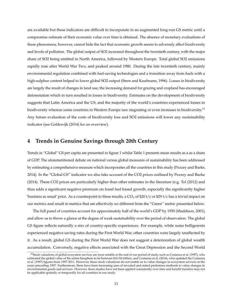
are available but these indicators are difficult to incorporate in an augmented long-run GS metric until a

compromise estimate of their economic value over time is obtained. The absence of monetary evaluations of

these phenomena, however, cannot hide the fact that economic growth seems to adversely affect biodiversity

and levels of pollution. The global output of SO2 increased throughout the twentieth century, with the major

share of SO2 being emitted in North America, followed by Western Europe. Total global SO2 emissions

rapidly rose after World War Two, and peaked around 1980. During the late twentieth century, mainly

environmental regulation combined with fuel-saving technologies and a transition away from fuels with a

high-sulphur content helped to lower global SO2 output (Stern and Kaufmann, 1996). Losses in biodiversity

are largely the result of changes in land use; the increasing demand for grazing and cropland has encouraged

deforestation which in turn resulted in losses in biodiversity. Estimates on the development of biodiversity

suggests that Latin America and the US, and the majority of the world’s countries experienced losses in

biodiversity whereas some countries in Western Europe saw stagnating or even increases in biodiversity.15

Any future evaluation of the costs of biodiversity loss and SO2 emissions will lower any sustainability

indicator (see Goldewijk (2014) for an overview).

4 Trends in Genuine Savings through 20th Century

Trends in “Global” GS per capita are presented in figure 1 whilst Table 1 presents mean results as a as a share

of GDP. The aforementioned debate on national versus global measures of sustainability has been addressed

by estimating a comprehensive measure which incorporates all the countries in this study (Pezzey and Burke,

2014). In the “Global GS” indicator we also take account of the CO2 prices outlined by Pezzey and Burke

(2014). These CO2 prices are particularly higher than other estimates in the literature (e.g. Tol (2012) and

thus adds a significant negative premium on fossil fuel based growth, especially the significantly higher

‘business as usual’ price. As a counterpoint to these results, a CO2 of $20 t/c or $29 t/c has a trivial impact on

our metrics and result in metrics that are effectively no different from the “Green” metric presented below.

The full panel of countries account for approximately half of the world’s GDP by 1950 (Maddison, 2001),

and allow us to throw a glance at the degree of weak sustainability over the period of observation. The global

GS figure reflects naturally a mix of country-specific experiences. For example, while some belligerents

experienced negative saving rates during the First World War, other countries were largely unaffected by

it. As a result, global GS during the First World War does not suggest a deterioration of global wealth

accumulation. Conversely, negative effects associated with the Great Depression and the Second World

15Stock valuations of global ecosystem services are most notable at the end of our period of study, such as Costanza et al. (1997), whoestimated the global value of the entire biosphere to be between $16-54 trillion, and Costanza et al. (2014), who updated the Costanzaet al. (1997) figures from 1997-2011. However, these stock valuations do not enable us to value changes in ecosystem services in theyears preceding 1997. Furthermore, there have been increasing uses of revealed and stated preference methods to value changes inenvironmental goods and services. However, these studies have not been applied consistently over time and benefit transfers may notbe applicable spatially or temporally for all countries in our study.

11

Figure 1: Global estimations on Net Investment, Green Investment, GS and GSTFP per capita. GK$ 1990.Co2 Estimations with prices under control ($131 in 2005) and no control ($1455 in2005)

-1000

0

1000

2000

3000

4000

5000

1900 1920 1940 1960 1980 2000

Gea

ry K

ham

is $

1990

per

cap

ita

Co2 under control $ 131

NetGreen

GreenCO2GS

GSTFPGreenTFP

-2500

-2000

-1500

-1000

-500

0

500

1000

1500

2000

2500

3000

1900 1920 1940 1960 1980 2000

Gea

ry K

ham

is $

1990

per

cap

ita

Co2 under no control $ 1455

NetGreen

GreenCO2GS

GSTFPGreenTFP

Sources: Own estimations-Data appendix table 3 and table 4

12

War are clearly visible in the global GS figure; these two periods were the only episodes in the twentieth

century when the world experienced substantial losses of wealth. In the aftermath of the Second World

War, global GS recovered quickly, rising to unprecedented levels in the 1970s. Starting with the economic

depression in the 1980s, GS decreased to somewhat lower levels, but remained to be consistently high in

historical perspective. Although towards the end of our sample represents a declining share of global GDP

(40 per cent by 1990) and thus weakens the global representativeness of our findings.

Table 1: Global Net Investment, Green, Genuine Savings and GSTFP as share of the GDP

CO2 Prices under control US$131 (2005) CO2 Prices under no control US$1455 (2005)

Net Investment Green GreenCo2 GS GSTFP GreenTFP GreenCo2 GS GSTFP GreenTFP% % % % % % % % % %

7,39 4,97 3,74 6,88 33,01 30,08 -8,61 -5,47 20,80 17,861900-1946

CO2 Prices under control US$131 (2005) CO2 Prices under no control US$1455 (2005)Net Investment Green GreenCo2 GS GSTFP GreenTFP GreenCo2 GS GSTFP GreenTFP

% % % % % % % % % %7,47 4,97 3,94 5,69 32,93 31,19 -6,50 -4,75 22,50 20,75

1946-2000CO2 Prices under control US$131 (2005) CO2 Prices under no control US$1455 (2005)

Net Investment Green GreenCo2 GS GSTFP GreenTFP GreenCo2 GS GSTFP GreenTFP% % % % % % % % % %

7,33 4,96 3,58 7,88 33,09 28,94 -10,38 -6,08 19,05 14,91

Sources: Own estimations in based to the Appendix

In a counterfactual study of how much countries would be wealthier in terms of fixed capital if they

followed the Hartwick Rule and reinvested in fixed capital, Hamilton et al. (2006) illustrate the possibility

of unbounded and rising consumptionif a GS rate of at least 5 per cent of GDP was maintained over time.

Hamilton et al. (2006)’s finding provides us with a yardstick with which to assess the performance of our

global metric from a sustainability perspective in terms of its capacity for raising consumption over future

generations. For our ‘global’ indicator, Table 1 shows that net investment is overwhelmingly positive which

indicates that rents were reinvested in the productive capacities. However, in terms of Green investment,

this is considerably lower and over the whole century this is below the 5% prescribed threshold outlined

by Hamilton et al. (2006). When CO2 damages are accounted for this suggests a worse performance and

although this metric is not negative, CO2 damages are large and rising over the 20th century and are likely

to increase in the future. Our GS indicator, which includes education expenditure, returns our sustainability

indicator towards a sustainability path and GSTFP even more so. The message appears to be clear, the

20th century shows that overall the Hartwick Rule was followed but worries about the legacy of CO2

emissions are clearly evident. CO2 damages clearly indicate a path towards lower “green savings”. Yet,

taking a sanguine view, if we continue to adopt technological solutions we may continue on a sustainable

13

development path.

The data presented in Table 2 and Figures 2, 3 and 4 illustrate the patterns of our respective countries,

although we have opted to exclude CO2 from these metrics. Net investment in our panel of Western countries

was generally positive, ranging from approximately five per cent in Great Britain, between seven and ten

per cent in the United States, Australia, France, and Germany, to approximately 14 per cent in Switzerland.

Resource depletion played a modest role among these countries, with Australia and the US depleting natural

resources in the amount of 3.4 and 2.7 per cent of GDP, respectively. British and Germany depletion levels

were between one and two per cent of GDP, while French depletion totals 0.6 per cent of GDP. Switzerland, a

country almost without any significant natural resources, accumulated natural capital due to the absence

of depletion of fossil fuels and minerals and afforestation. Our panel of Western countries was relatively

homogenous in terms of education expenditure; figures range from 2.2 to 3.7 per cent of GDP.

However, by far the largest single contributor to wealth accumulation was through the value of techno-

logical progress. Technology is broadly defined, including human capital, social capital, but also the quality

of formal and informal institutions; it is proxied as total factor productivity and it captures productive factors

that are not included in physical capital and labour inputs. Our augmented GS indicator, which is inspired by

Weitzman (1997), includes the accumulation of physical capital, pollution, resource depletion as well as the

present value of future changes in technology. Our results suggest that technology is an important intangible

asset, contributing 17 and 18 per cent of GDP to national savings in France and Australia, respectively, 23 and

25 per cent in Great Britain and the US, respectively, 28 per cent in Switzerland and 38 per cent in Germany.

The development of GS in the panel of Western countries mirrors the political and social history during

this period (figure 2). Important events influencing economic development include the two World Wars, the

Great Depression during the interwar years, and the depression during the early 1980s. These events are

clearly visible in the data, but the magnitude of the associated economic effects suggest that these shocks

were experienced differently across these six Western countries. War economies during the First World

War resulted in negative GS in Great Britain, France, Australia and Germany, while GS in the United States

remained almost unaffected. Similarly, Great Britain, the United States, France and in particular Germany

experienced negative GS rates during the Second World War. These effects mirror the extraordinary war

effort and the absence of any long-run development strategy; the consequences of the Second World War

was most devastating in Germany, which suffered heavily due to dismantlement and destruction of capital,

but other European warring parties were also seriously affected. Conversely, Australia during the Second

World War, and neutral Switzerland throughout this troubled period benefitted from the turmoil in terms of

GS. A somewhat atypical pattern is visible in the Swiss GS series. While the two World Wars and the Great

Depression slowed wealth accumulation down considerably in many countries, Switzerland experienced

large savings during these period. It is important to highlight Switzerland’s role as a safe haven of capital,

14

and the limited possibilities of import and domestic consumption during these periods.

Western countries in this panel developed rapidly during the post-war Golden Age, both in terms of

economic growth but also in terms of GS. Between 1950 and 1970, GS in the United States and Great Britain

almost doubled, French and German GS almost tripled, and Swiss GS more than quadrupled. The exception

to this rule is Australia, where GS were constantly positive, but by and large stagnated during this period.

Only during the 1970s and early 1980s, Australia experienced increases in GS. The global recession of the

early 1980s is also visible in the development of GS; Great Britain and the United States experienced the

largest decline in GS during this period.

In figure 2 we present the augmented GS estimate, which captures changes in the value of technology in

an economy in addition to conventional GS. During the first half of the 20th century, we find that a large

share of wealth is generated through the accumulation of technology, not through conventional GS. The

upper trend in each country diagram reports the level of Genuine Savings including the present value of

future changes in technology. This development is reinforced during the second half of the 20th century,

when technology becomes a large contributor to wealth accumulation. In the United States, Great Britain

and Germany, technology becomes the largest single contributor to wealth accumulation during this period.

By 1950, augmented GS in these three countries is three to four times larger than the conventional GS metric.

In France and Australia, technology also plays an important role with respect to wealth accumulation, but

levels of GS and augmented GS are evidently lower than in the US, Great Britain and Germany. Switzerland,

again, shows some atypical patterns regarding the role of accumulation of intangible assets. Swiss GS and

augmented GS increased rapidly during the 20th century, but this increase seems to be the result of physical

capital accumulation; the present value of future changes in technology appears to remain almost constant

across time.

Results for Latin America suggest that net investment during the twentieth century was somewhat lower

compared with Western countries’ wealth accumulation. However, net investment was considerable in

Brazil, Colombia and Mexico, almost reaching Western levels (table 2). Whereas net investment in Argentina

and Chile was relatively low in comparison, but positive on average. The most striking difference between

Latin American countries and the set of Western countries is the generally low levels of augmented saving

measures. If resource depletion is incorporated in the green investment indicator, savings are substantially

lower, and reach negative values for Chile and Mexico. Similarly, Brazilian and Colombian investment

figures drop from eleven and nine per cent to approximately 4 per cent each when resource depletion

is considered. In Chile, depletion can be mainly attributed to copper ore and saltpetre depletion, while

Colombia and Mexico have been producers of petroleum. Resource depletion is partly outweighed by

investment in education; the value of education expenditure ranges between under 0.5 per cent of GDP

(Argentina) to up to 1.7 per cert (Brazil). Moreover, with lower TFP growth, technological progress accounts

15

Table 2: Net Investment, Green, Genuine Savings and GSTFP as share of GDP

1900 - 2000

Net Investment Green GS GSTFP% % % %

Britain 4,63 2,80 5,49 28,58Germany 9,41 8,09 11,34 49,57US 7,07 4,42 8,11 32,62Australia 7,68 4,33 6,55 24,69France 8,93 8,38 11,76 29,07Switzerland 14,07 14,39 17,53 45,40Argentina 3,73 3,20 3,54 13,67Brazil 11,10 3,88 5,71 27,29Chile 2,06 -5,64 -3,75 1,82Colombia 8,73 3,61 4,69 6,98Mexico 8,58 -1,40 -0,30 7,24

1900-1946

Net Investment Green GS GSTFP% % % %

Britain 2,64 0,86 2,42 20,80Germany 9,47 8,01 10,12 49,25US 9,30 6,27 8,29 38,02Australia 7,59 4,59 5,51 25,09France 5,16 4,69 6,26 35,54Switzerland 11,47 11,80 13,90 54,29Argentina 3,56 3,40 3,59 16,58Brazil 12,96 3,29 4,20 14,17Chile 3,85 -1,67 -0,64 3,14Colombia 1,48 -3,38 -3,05 -0,69Mexico 2,42 -11,42 -10,93 -5,85

1900-1946

Net Investment Green GS GSTFP% % % %

Britain 6,29 4,43 8,07 35,08Germany 9,35 8,16 12,36 49,83US 5,21 2,88 7,96 34,36Australia 7,75 4,11 7,42 24,35France 12,09 11,47 16,35 23,66Switzerland 16,24 16,56 20,57 37,95Argentina 3,87 3,02 3,50 11,24Brazil 9,59 4,43 7,05 38,53Chile 0,56 -8,96 -6,36 0,72Colombia 14,80 9,45 11,17 13,40Mexico 13,73 6,97 8,60 18,20

Source: Own estimations and Data Appendix

16

Figure 2: Genuine Savings and augmented Genuine Savings with TFP per capita.Developed Countries 1900 - 2000, Geary -Khamis $ 1990

-2000

0

2000

4000

6000

8000

1900 1920 1940 1960 1980 2000

Gea

ry-K

ham

is $

1990

GREAT BRITAIN

GS GSTFP

-2000

0

2000

4000

6000

8000

1900 1920 1940 1960 1980 2000

Gea

ry-K

ham

is $

1990

UNITED STATES

GSGSTFP

-2000

0

2000

4000

6000

8000

1900 1920 1940 1960 1980 2000

Gea

ry-K

ham

is $

1990

GERMANY

GSGSTFP

-2000

0

2000

4000

6000

8000

1900 1920 1940 1960 1980 2000

Gea

ry-K

ham

is $

1990

FRANCE

GSGSTFP

-2000

0

2000

4000

6000

8000

1900 1920 1940 1960 1980 2000

Gea

ry-K

ham

is $

1990

AUSTRALIA

GSGSTFP

-2000

0

2000

4000

6000

8000

1900 1920 1940 1960 1980 2000

Gea

ry-K

ham

is $

1990

SWITZERLAND

GSGSTFP

Source, Appendix

for only 2 per cent of GDP in Colombia, between 10 and 20 per cent in Argentina and Brazil, approximately

five-seven per cent of GDP in Chile and Mexico.

Figure 4 allows a closer look at the development of investment in Latin America, including the effects

of social turmoil and somewhat higher investment rates in the second half of 20th century. We cannot

identify a clear trend in the development of GS during the first half of the 20th century; in fact, we by and

large observe long periods of stagnation, which were interrupted by the First World War, the Second World

War and to a lesser extend by the Great Depression. Latin American economies, however, were generally

less affected by these events compared with some Western countries. The Mexican Revolution resulted in

highly negative GS during the Revolution, 1910 to 1920, and its aftermath. Mexican GS turned positive only

during the Second World War. The second half of the 20th century generally brought somewhat higher GS,

and some Latin American economies experienced a sustained increase in savings. Decisive events in this

period include capital flight after 1970, and the Chilean depression after 1972, which were related to socialist

reforms. Chilean GS recovered slowly, only reaching positive saving rates in the early 1980s. The global

17

Figure 3: Genuine Savings TFP augmented in GK $1990 per capita. Developed countries 1900 - 1990

-1000

0

1000

2000

3000

4000

5000

6000

7000

8000

9000

10000

1900 1910 1920 1930 1940 1950 1960 1970 1980 1990

Gea

ry K

ham

is $

1990

years

GREAT BRITAIN

-1000

0

1000

2000

3000

4000

5000

6000

7000

8000

9000

10000

1900 1910 1920 1930 1940 1950 1960 1970 1980 1990

Gea

ry K

ham

is $

1990

years

USA

-1000

0

1000

2000

3000

4000

5000

6000

7000

8000

9000

10000

1900 1910 1920 1930 1940 1950 1960 1970 1980 1990

Gea

ry K

ham

is $

1990

years

GERMANY

-1000

0

1000

2000

3000

4000

5000

6000

7000

8000

9000

10000

1900 1910 1920 1930 1940 1950 1960 1970 1980 1990

Gea

ry K

ham

is $

1990

years

AUSTRALIA

-1000

0

1000

2000

3000

4000

5000

6000

7000

8000

9000

10000

1900 1910 1920 1930 1940 1950 1960 1970 1980 1990

Gea

ry K

ham

is $

1990

years

SWITZERLAND

-1000

0

1000

2000

3000

4000

5000

6000

7000

8000

9000

10000

1900 1910 1920 1930 1940 1950 1960 1970 1980 1990

Gea

ry K

ham

is $

1990

years

FRANCE

Source, Appendix

18

Figure 4: Genuine Savings TFP augmented in GK $1990 per capita. Latin American countries 1900 - 1990

-1500

-1000

-500

0

500

1000

1500

2000

2500

3000

3500

1900 1920 1940 1960 1980 2000

Gea

ry K

ham

is $

1990

years

ARGENTINA

-1500

-1000

-500

0

500

1000

1500

2000

2500

3000

3500

1900 1920 1940 1960 1980 2000

Gea

ry K

ham

is $

1990

years

BRAZIL

-1500

-1000

-500

0

500

1000

1500

2000

2500

3000

3500

1900 1920 1940 1960 1980 2000

Gea

ry K

ham

is $

1990

years

CHILE

-1500

-1000

-500

0

500

1000

1500

2000

2500

3000

3500

1900 1920 1940 1960 1980 2000

Gea

ry K

ham

is $

1990

years

COLOMBIA

-1500

-1000

-500

0

500

1000

1500

2000

2500

3000

3500

1900 1920 1940 1960 1980 2000

Gea

ry K

ham

is $

1990

years

MEXICO

Source, Appendix

19

recession of the early 1980s, and especially the depression of Asian economies in the late 1990s, affected

Latin America, leading to plummeting investment.

5 Conclusions

This study provides estimates of the development of a series of ‘Global’ and national savings metrics using a

panel of eleven countries in the course of the twentieth century. We compare net investment, GS, and an

augmented GS measure that considers the value of technology, to assess the degree of weak sustainability of

these countries. We find that GS were mostly positive during this period and increased substantially during

the second half of the twentieth century. The results for six Western countries in our panel - Australia, France,

Germany, Great Britain, Switzerland, and the United States - suggest that the Western world experienced

large accumulation of capital, and that a large share of this capital accumulation occurred due to intangible

assets, such as technology. For Latin America, we find that physical capital accumulation was largely positive

during the twentieth century. However, most Latin American countries in our panel experienced substantial

depletion of natural resources, and this disinvestment reduces national savings considerably. The eventful

history of the twentieth century left severe marks, which are reflected by investment and savings figures

presented in this study. The First World War is the first of these events in the twentieth century; it resulted in

plummeting savings rates among European warring parties. The Great Depression, which is considered

one of the most severe depressions in history, had a similar impact among the affected countries. The most

devastating effect, however, came about during the Second World War, when a great deal of economic

resources were invested in the war effort, and long-run development strategies were largely absent. The

second half of the twentieth century brought substantial increases in wealth accumulation, especially in

Western countries, but also setbacks during the Oil Crisis in the 1970s and the global economic depression

in the early 1980s. However, we find that the treatment of CO2 and how it is priced has an enormous

impact on the sustainability signal (Pezzey and Burke (2014). The two prices shown, the high ‘business

as usual’ and the lower ‘control’, highlight the messages embodied in their assumptions: if there are no

attempts to control emissions into the future, then the twentieth century was a century built on unsustainable

practices; if, however, the damaging potential of uncontrolled emissions are accepted and these emissions

are optimally ‘controlled’, then the development seen in the twentieth century can be determined to have

been on a sustainable path. Only time can tell. Why do these events matter? The results presented in

this chapter have strong implications for the present and future economic development of the countries

considered in this study. A number of studies argue that consumption is a function of (previous) capital

accumulation, since the productive basis, i.e. labour, physical and intangible capital, are the productive

forces used to generate income. The lessons from these studies are straightforward: current investment in

20

physical capital, intangible assets such as human capital and technology may result in higher consumption,

wages and well-being in the future. Likewise, erosion of the productive basis due to depreciation of assets,

pollution and depletion of natural resources may limit, or even reduce, future well-being. The implications

of this perspective for the ‘global’ economy are clear; in order to ensure future sustainability the Hartwick

Rule ought to be followed and technological progress, i.e. an increasingly intelligent use of existing assets,

can play an immense role in future sustainability, especially taking into account the future development of

the new economic giants of twenty-first century (i.e. China and India).

Bibliography

Arrow, K. J., P. Dasgupta, L. H. Goulder, K. J. Mumford, and K. Oleson (2012, may). Sustainability and the measurement

of wealth. Environment and Development Economics 17(03), 317–353.

Atkinson, G., M. Agarwala, and P. Muñoz (2012). Are national economies (virtually) sustainable?: an empirical analysis of

natural assets in international trade. In Inclusive Wealth Report 2012: Measuring progress toward sustainability, Volume 1,

pp. 87–117. Cambridge University Press.

Baier, S. L., G. P. Dwyer, and R. Tamura (2006). How important are capital and total factor productivity for economic

growth? Economic Inquiry 44(1), 23–49.

Bértola, L. and J. A. Ocampo (2012). The Economic Development of Latin America Since Independence. Initiative for Policy

Dialogue. (Oxford: Oxford University Press).

Blum, M., E. McLaughlin, and N. Hanley (2013). Genuine savings and future well-being in Germany, 1850-2000.

Bolt, J. and J. L. van Zanden (2014, mar). The Maddison Project: collaborative research on historical national accounts.

The Economic History Review, n/a–n/a.

Bolt, K., M. Matete, and M. Clemens (2002). Manual for calculating adjusted net savings. Environment Department, World

Bank, 1–23.

Camacho, C. (2014). Adjusted Net Savings and its Relationship with Future Well-being: Policy Implications for Latin America.

Msc thesis, TU Munich.

Costanza, R., R. d’Arge, R. De Groot, S. Faber, M. Grasso, B. Hannon, K. Limburg, S. Naeem, R. V. O’neill, J. Paruelo,

et al. (1997). The value of the world’s ecosystem services and natural capital. Nature.

Costanza, R., R. de Groot, P. Sutton, S. van der Ploeg, S. J. Anderson, I. Kubiszewski, S. Farber, and R. K. Turner (2014).

Changes in the global value of ecosystem services. Global Environmental Change 26, 152–158.

Feinstein, C. (1972). National Income, Expenditure and Output of the United Kingdom, 1855-1965. Cambridge: Cambridge

University Press.

21

Feinstein, C. H. and S. Pollard (Eds.) (1988). Studies in Capital Formation in the United Kingdom, 1750-1920. Oxford

University Press.

Ferreira, S., K. Hamilton, and J. R. Vincent (2008). Comprehensive wealth and future consumption: Accounting for

population growth. World Bank Economic Review 22(2), 233–248.

Ferreira, S. and M. Moro (2011). Constructing genuine savings indicators for Ireland, 1995-2005. Journal of Environmental

Management 92(3), 542–53.

Ferreira, S. and J. R. Vincent (2005). Genuine Savings : Leading Indicator of Sustainable Development ? Economic

Development and Cultural Change 53(3), 737–754.

Goldewijk, K. K. (2014). Environmental quality since 1820. In Z. Luiten, B. Joerg, M. Marco, R. Auke, and T. Marcel

(Eds.), How was life? Global Well-being Since 1820, Chapter 10. OECD Publishing.

Gómez-Galvarriato, A. and W. J.G. (2009). Was It Prices, Productivity or Policy? Latin American Industrialisation after

1870. Journal of Latin American Studies 41(04), 663–694.

Gordon, R. (2016). The Rise and Fall of American Growth: The U.S. Standard of Living since the Civil War. The Princeton

Economic History of the Western World. Princeton University Press.

Greasley, D., N. Hanley, J. Kunnas, E. McLaughlin, L. Oxley, and P. Warde (2014). Testing genuine savings as a

forward-looking indicator of future well-being over the (very) long-run. Journal of Environmental Economics and

Management 67(2), 171–188.

Greasley, D., N. Hanley, E. McLaughlin, and L. Oxley (2016). Australia: a Land of Missed Opportunities?, st andrews

environmental economics discussion papers, 2016-08.

Hamilton, K. (1994). Green adjustments to GDP. Resources Policy 20(3), 155–168.

Hamilton, K. and M. Clemens (1999, may). Genuine Savings Rates in Developing Countries. The World Bank Economic

Review 13(2), 333–356.

Hamilton, K. and C. Hepburn (2014, may). Wealth. Oxford Review of Economic Policy 30(1), 1–20.

Hamilton, K., G. Ruta, and L. Tajibaeva (2006). Capital accumulation and resource depletion: A hartwick rule counterfac-

tual. Environmental and Resource Economics 34(4), 517–533.

Hanley, N., L. Dupuy, and E. Mclaughlin (2015). Genuine savings and sustainability. Journal of Economic Surveys 29(4),

779–806.

Hanley, N., L. Oxley, D. Greasley, E. McLaughlin, and M. Blum (2016). Empirical Testing of Genuine Savings as

an Indicator of Weak Sustainability: A Three-Country Analysis of Long-Run Trends. Environmental and Resource

Economics 63(2), 313–338.

22

Hartwick, J. (1977). Intergenerational equity and the investing of rents from exhaustible resources. The american economic

review.

Höfeler, T. (2014). Evaluating sustainable economic development in Latin America in historical perspective. Msc thesis, TU

Munich.

Klenk, C. (2013). Green accounting in a historical framework – The power of genuine saving rates as a forecasting instrument for

future well-being. Msc thesis, TU Munich.

Koch, N., S. Fuss, G. Grosjean, and O. Edenhofer (2014). Causes of the EU ETS price drop: Recession, CDM, renewable

policies or a bit of everything?-New evidence. Energy Policy 73, 676–685.

Kunnas, J., E. McLaughlin, N. Hanley, D. Greasley, L. Oxley, and P. Warde (2014). Counting carbon: historic emissions

from fossil fuels, long-run measures of sustainable development and carbon debt. Scandinavian Economic History

Review 62(3), 243–265.

Lindmark, M. and S. Acar (2013, feb). Sustainability in the making? A historical estimate of Swedish sustainable and

unsustainable development 1850–2000. Ecological Economics 86, 176–187.

Maddison, A. (2001). The World Economy: A Millennial Perspective. OECD.

Manuelli, R. E. and A. Seshadri (2014). Human capital and the wealth of nations. The American Economic Review 104(9),

2736–2762.

Markandya, A. and S. Pedroso-Galinato (2007). How substitutable is natural capital? Environmental and Resource

Economics 37(1), 297–312.

Mennig, P. (2015). Genuine Savings and Future Well-Being in France, 1850-2000. Msc thesis, TU Munich.

Mota, R. P. and T. Domingos (2013, nov). Assessment of the theory of comprehensive national accounting with data for

Portugal. Ecological Economics 95, 188–196.

Pearce, D. (2002). An Intellectual History of Environmental Economics. Annual Review of Energy and the Environment 27,

57–81.

Pearce, D. W. and G. D. Atkinson (1993). Capital theory and the measurement of sustainable development: an indicator

of "weak" sustainability. Ecological Economics 8(2), 103–108.

Pemberton, M. and D. Ulph (2001). Measuringincome and measuring sustainability. Scandinavian Journal of Eco-

nomics 103(1), 25–40.

Pezzey, J. (2004). ‘one-sided sustainability tests with amenities, and changes in technology, trade and population’. Journal

of Environmental Economics and Management 48(1), 613–631.

Pezzey, J. C. and P. J. Burke (2014, oct). Towards a more inclusive and precautionary indicator of global sustainability.

Ecological Economics 106, 141–154.

23

Pezzey, J. C., N. Hanley, K. Turner, and D. Tinch (2006, apr). Comparing augmented sustainability measures for Scotland:

Is there a mismatch? Ecological Economics 57(1), 60–74.

Prados de la Escosura, L. (2009). When did Latin America fall behind? In The Decline of Latin American Economies: Growth,

Institutions, and Crises. University of Chicago Press.

Rostow, W. W. (1960). The stages of economic growth. Cambridge University Press.

Rubio, M. d. M. (2004). The capital gains from trade are not enough: evidence from the environmental accounts of

Venezuela and Mexico. Journal of Environmental Economics and Management 48(3), 1175–1191.

Sachs, J. D. (1999). Resource Endowments and the Real Exchange Rate: A Comparison of Latin America and East Asia.

In Changes in Exchange Rates in Rapidly Developing Countries: Theory, Practice, and Policy Issues (NBER-EASE volume 7),

NBER Chapters, Chapter 5, pp. 133–154. National Bureau of Economic Research, Inc.

Sachs, J. D. and A. M. Warner (2001). The curse of natural resources. European Economic Review 45(4 - 6), 827–838.

Stern, D. I. and R. K. Kaufmann (1996). Estimates of global anthropogenic methane emissions 1860–1993. Chemo-

sphere 33(1), 159–176.

Stern, N. (2007). Economics of Climate Change: The Stern Review. Cambridge University Press.

Stiglitz, J. E., A. Sen, and J.-P. Fitoussi (2009). Report by the Commission on the Measurement of Economic Performance

and Social Progress. Sustainable Development 12, 292.

Tafunell, X. and C. Ducoing (2015, oct). Non-Residential Capital Stock in Latin America, 1875-2008: New Estimates and

International Comparisons. Australian Economic History Review, n/a–n/a.

Tol, R. S. J. (2012). On the Uncertainty About the Total Economic Impact of Climate Change. Environmental and Resource

Economics 53(1), 97–116.

UNU-IHDP. (2012). Inclusive wealth report 2012: measuring progress toward sustainability. Cambridge University Press.

UNU-IHDP. (2014). Inclusive wealth report 2014: measuring progress toward sustainability. Cambridge University Press.

Vincent, J. R. (2001). Are greener national accounts better?, centre for international development at harvard university working

papers 63.

Weitzman, M. L. (1997, mar). Sustainability and Technical Progress. Scandinavian Journal of Economics 99(1), 1–13.

Weitzman, M. L. (1999). Pricing the limits to growth from minerals depletion. Quarterly Journal of Economics, 691–706.

World Bank (1997). Expanding the Measure of Wealth: Indicators of Environmentally Sustainable Development.

World Bank (2006). Where is the Wealth of Nations?: Measuring Capital for the 21st Century. The World Bank.

World Bank (2011). The Changing Wealth of Nations: Measuring Sustainable Development in the New Millennium. World Bank

Publications.

24

World Bank (2015). World Development Indicators 2015.

World Commission on Environment and Development (1987). Report of the World Commission on Environment and

Development: Our Common Future (The Brundtland Report).

25

Appendix

Sources

Australia

The GS estimations for Australia: Greasley et al. (2016)

Great Britain and United States

Hanley et al. (2016)

France

Note that all statistics use for this study refer to ‘European France’, excluding Algeria and other (former) colonies.

GDP and GDP deflator: Pre-1982 data on French GDP is available from Toutain (1987) and Flora et al. (1983). GDP

levels for later periods are taken from official Statistical Yearbooks of the French National Institute of Statistics and

Economic Studies (INSEE). Data for the period between 1914 and 1920 can be found in Hautcoeur (2005). For the

period 1939 to 1945 data on French GDP is taken from Occhino, Oosterlinck and White (2006). A GDP deflator was

constructed using data from Mitchell (2007), Lévy-Leboyer and Bourguignon (1985) and the INSEE. Net investment: net

fixed capital formation and changes in inventories for the 19th and for the beginning of the 20th century is provided by

Lévy-Leboyer and Bourguignon (1985). The gap between 1914 and 1945 was estimated using Markovitch (1966) who

reports investment and destructions during the wars as well as investment in the inter-war period and Carré, Dubois

and Malinvaud (1972). For the period 1945 to 2000 data on inventory changes and net fixed capital formation was taken

from the INSEE, the World Bank (2014) and the United Nations UNSD (2014) investment statistics. Data on net overseas

investment is provided by Banque de France (2014), which provides a section with historical time series going back to

the 18th century. Private consumption was taken from Flora et al. (1983), the INSEE, Baudrillard (1996), Beaupré (2004)

and Asselain (1984). Forestry: For the second half of the 19th century a complete time series of French forest stocks and

the French timber market was not available. In France, forestry management only developed to a high standard at the

end of the 19th century. Therefore, linear interpolation was used for the construction of the time series between 1850 and

1890 as there was only data available in five year intervals. Information on French forestry stocks were taken from Zon

(1910) and Zon and Sparhawk (1923), Cinotti (1996), Koerner et al. (2000) and from the statistical database of the FAO

(2014). Non-renewable resources: Detailed data on French mining activities, including the number of employees in the

mining sector, extraction quantities and market prices, can be found in the yearly publications of the French mining

sector called Les Annales des Mines, a series of which the first issue was published in 1794. Additional information

are provided by the statistical yearbooks of the INSEE, especially by the issues called Annuaires Rétrospectifs, which

include data going back until the 18th century, and by Mitchell (2007). To assess the costs of depletion the number

of employees in the mining sector and their average wage were used. Data on the labour force is provided by Les

Annales des Mines and the INSEE. Wages of mining workers are reported by the INSEE, Simiand (1907), Marchand

and Thélot (1997) and Diebolt and Jaoul-Grammare (2008). Education expenditure is provided by Diebolt (1995, 2000).

26

For the post-1994 period World Bank (2014) data on education expenditure was used. Carbon emissions were taken

from Andres et al. (1999) and Boden, Marland and Andres (1995). This data is available online on the website of the

Carbon Dioxide Information Analysis Center, an organization within the United States Department of Energy, under

http://cdiac.ornl.gov/CO2_Emission/timeseries/national. Total Factor Productivity: labour hours worked and real

GDP is taken from Greasley and Madsen (2006). Information on capital stock can be found in Guerrero (2013). Factor

shares used were from Greasley and Madsen (2006), capital share is 0.60 and labour 0.40. A Kalman filter of the TFP

growth rate was estimated and this was forecast using an ARIMA (2,1). Discount rates: Data on historical interest rates

and government bond yields were taken from Homer and Sylla (2005) and Banque de France (2014).

Germany

GDP and GDP deflator: Pre-1975 data on German national product is available from Flora et al. (1983) and Hoffmann

et al. (1965). GDP levels for later periods are taken from German Statistical Yearbooks (1999, 2008). Missing periods

1914-1924 and 1940-1949 were estimated using Ritschl and Spoerer’s (1997) GNP series. A GDP deflator was constructed

using data from Hoffman et al (1965), Mitchell (2007) and the United Nations Statistical Division (2013). Net investment:

Net investment from 1850-1959 is provided by Hoffmann et al. (1965). We estimated the gap during 1914-1924 using

Kirner (1968) who reports investment in buildings, construction, and equipment by sector for the war and inter-war

periods. The period 1939 to 1949 was estimated by using data on net capital stock provided by Krengel (1958). To

estimate investment during 1960 to 1975 we used Flora et al.’s (1983) data on net capital formation. For the period 1976

to 2000 we use official World Bank (2010) and United Nations (2013) investment statistics to complete the series. Data on

the change in overseas capital stock and advances is provided by Hoffmann et al. (1965). Gaps during war and inter-war

periods were estimated using information on the balance of payments provided by the German central bank (Deutsche

Bundesbank, 1998, 2005). Remaining missing values were estimated using trade balances as a proxy for capital flows

(Deutsche Bundesbank, 1976; Flora et al., 1983; Hardach, 1973). Private Consumption is taken from Flora et al. (1983),

German Statistical Office, downloadable under www.gesis.oreg/histat, Ritschl (2005), Abelshauser (1998), and Harrison

(1988). Forestry: Zon (1910), Zon et al. (1923), Hoffmann et al. (1965), and Endres (1922). Non-renewable resources:

Fischer (1989) and Fischer and Fehrenbach (1995) provide detailed data on German mining activities including the

number of employees in mining, covering the period until the 1970s. Information on quantities and market prices by

commodity on an annual basis are available. Additional information was collected from Mitchell (2007). Data provided

by Fischer (1989) and Fischer and Fehrenbach (1995) are also available by German state, which allows subtracting

contemporary contributions of the mining sector of Alsace-Lorraine between 1871 and 1918. Moreover, the statistical

offices of the German Empire and the Federal Republic of Germany provide information on the 1914 to 1923 as well as

the post-1962 periods, respectively (Bundesamt, 2013; Germany. Statistisches Reichsamt., 1925). To assess the costs of

depletion the number of employees in mining and their average wage were used. Data on the labour force in mining is

provided by Fischer (1989), Fischer and Fehrenbach (1995), and the German Statistical Office (2013). Wages of mining

workers are reported by Hoffmann et al. (1965), Kuczynski (1947), Mitchell (2007), and official contemporary statistics

(Germany. Statistisches Reichsamt., 1925). Expenditure on schooling: Data on education expenditure is provided

by Hoffmann et al. (1965) and Diebolt (1997, 2000). For the post-1990 period we use World Bank data on education

27

expenditure. Missing values for the periods 1922-24 and 1938-48 have to be estimated. For the former period, we assume

that expenditures between 1921 and 1925 developed gradually and apply linear interpolation. For the latter period

we use Flora (1983, p. 585) who reports that the number of pupils and students in Germany dropped by 16.3 per cent

between 1936 and 1950 – this occurred most likely due to population losses after WWII. The corresponding drop in

education expenditure was 16.5 per cent. We assume that the 1939 expenditure level was maintained until 1945, when

the number of students plummeted. Therefore, we assume that the expenditure level between 1946 and 1948 was equal

to the 1949 figure. Carbon emissions were taken from Andres et al. (1999) and Boden et al. (1995). TFP: Data on labour

hours worked and real GDP is taken from Greasley and Madsen (2006). Information on capital stock for the period

1850 through 2000 is provided by Metz (2005). Missing values during and after WWII have been estimated on the basis

of Krengel (1958). Factor shares used were from Greasley and Madsen (2006), capital share is 0.60 and labour 0.40.

A Kalman filter of the TFP growth rate was estimated. Discount rates were taken from Homer and Sylla (2005) and

Deutsche Bundesbank (2013)[2].

Switzerland

GDP: Halbeisen et al (2012), Wirtschaftsgeschichte der Schweiz im 20. Jahrhundert. Basel: Schwabe; HSSO: His-

torische Statistik der Schweiz Online (Historical Statistics of Switzerland online), Kammerer Patrick et al. (Hg.),

www.fsw.uzh.ch/histstat/main.php.; Capital: Halbeisen et al. (2012); BFS Online: Swiss Statistics, Swiss Federal Statisti-

cal Office (BFS), www.bfs.admin.ch/; Kehoe and Ruhl (2003); Goldsmith (1981); Siegenthaler and Ritzmann-Blickenstorfer

(1996); Education expenditure: BFS Online: Swiss Statistics, Swiss Federal Statistical Office (BFS), www.bfs.admin.ch/;

HSSO: Historische Statistik der Schweiz Online (Historical Statistics of Switzerland online), Kammerer Patrick et al.

(Hg.), www.fsw.uzh.ch/histstat/main.php; Forest: HSSO: Historische Statistik der Schweiz Online (Historical Statistics

of Switzerland online), Kammerer Patrick et al. (Hg.), www.fsw.uzh.ch/histstat/main.php; Siegenthaler and Ritzmann-

Blickenstorfer (1996); BFS Online: Swiss Statistics, Swiss Federal Statistical Office (BFS), www.bfs.admin.ch/; LFI Online:

National forest inventory Switzerland LFI, http://www.lfi.ch/resultate/suche.php; Rieger (2007); Costs of production:

BAFU (2010). Biodiversität und Holznutzung – Synergien und Grenzen. Federal Office for the Environments Switzerland

(BAFU), April 2010; BAFU (2011). Jahrbuch Wald und Holz - Annuaire La forêt et le bois – Federal Office for the

Environments Switzerland (BAFU); Strawe (1994); HSSO: Historische Statistik der Schweiz Online (Historical Statistics

of Switzerland online), Kammerer Patrick et al. (Hg.), www.fsw.uzh.ch/histstat/main.php.; Degen (2012); BFS Online:

Swiss Statistics, Swiss Federal Statistical Office (BFS), www.bfs.admin.ch/; Studer (2008); Fossil fuel: Marek (2008); Marek

(1994); (Gisler, 2011); Gebhardt (1957); Bellwald (2013); BFS Online: Swiss Statistics, Swiss Federal Statistical Office (BFS),

www.bfs.admin.ch/ Iron ore: Fehlmann H. & Durrer R. (1932); HSSO: Historische Statistik der Schweiz Online (Histori-

cal Statistics of Switzerland online), Kammerer Patrick et al. (Hg.), www.fsw.uzh.ch/histstat/main.php.; IEA online:

International Energy Agency (IEA), http://www.iea.org/countries/membercountries/switzerland/; BFS Online: Swiss

Statistics, Swiss Federal Statistical Office (BFS), www.bfs.admin.ch/; Kündig and Leuenberger (1997); Bärtschi, 2011;

Gesis online, Historische Statistiken, Historical statistics (Histat): http://www.gesis.org/histat/; Population: BFS Online:

Swiss Statistics, Swiss Federal Statistical Office (BFS), www.bfs.admin.ch/; HSSO: Historische Statistik der Schweiz

Online (Historical Statistics of Switzerland online), Kammerer Patrick et al. (Hg.), www.fsw.uzh.ch/histstat/main.php.;

28

Discount rates: BFS Online: Swiss Statistics, Swiss Federal Statistical Office (BFS), www.bfs.admin.ch/; TFP: Halbeisen

et al, (2012).

Latin America

GDP and GDP deflator: Argentina – From 1900-2000 the nominal GDP was derived from Della Paolera and Taylor

(2003). GDP deflator is based on data from MoxLAD (2014) from 1900-1960 and on data from World Bank (2014b) for

years thereafter. Brazil – Nominal GDP and GDP deflator were derived from the historical series from IBGE (2014). Chile

– From 1900-1940 the nominal GDP in USD was calculated using Hofman (2000). From 1940-1995 the nominal GDP was

taken from Braun-Llona et al. (2000) and from 1995-2010 from Banco Central de Chile (2014). The GDP deflator was

derived from World Bank (2014b) from 1960-2010. Braun-Llona et al. (2000) reports a real GDP series from 1900-1995 in

prices from 1995. Colombia – The nominal GDP was taken from GRECO (1999b) from 1905-1997 and from 1998-2010 from

World Bank (2014b). For the years before 1905 the GDP was calculated using the growth rate reported by Hofman (2000).

From 1900-1960 the GDP deflator was derived by using the variations given by GRECO (1999b), after 1960 is it taken

from World Bank (2014b). Mexico – From 1900-1970 the nominal GDP was taken from INEGI (2009), following years are

derived from World Bank (2014b). The GDP deflator was calculated using the GDP deflator reported by MoxLAD (2014).

Consumer price index and inflation: Argentina, Brazil, Mexico – data were taken from Clio infra (2014). Chile – 1900-1995

from Braun-Llona et al. (2000); from 1995 and thereafter from Clio infra (2014). Colombia – 1900-1905 from Braun-Llona

et al. (2000) and from 1905 to 1996 data is from GRECO (1999b). For the last years it was taken from World Bank (2014b).

Exchange rates and changes in local currency units (LCU): Argentina – data from Della Paolera and Taylor (2003). The

exchange rate from Nuevos Pesos to USD from 1916 until 1999 was taken from Della Paolera and Taylor (2003) and for

later years from Clio infra (2014). Brazil – Changes in LCU were derived from MoxLAD (2014); the exchange rate from

LCU to USD from IBGE (2014). Chile – Changes in LCU are reported by MoxLAD (2014). From 1900-1995 the exchange

rate to USD is reported by Braun-Llona et al. (2000), while later years were taken from Banco Central de Chile (2014).

Colombia – exchange rate from Pesos to USD was taken from GRECO (1999b) from 1905-1997; for the following years it is

from CEPAL (2014). Mexico – Changes in LCU were taken from MoxLAD (2014); the exchange rate to USD was derived

from INEGI (2009) until 2009, while later years are from CEPAL (2014). Investment and gross fixed capital formation

(GFCF) – All countries – The series for GFCF after 1950 was taken from CEPAL (2009) and CEPAL (2014). These data

was converted to real prices of 2010 and calculated for the years from 1900-1950 using the index reported by Tafunell

(2011). Tafunell (2013) explains the method to build the GFCF data on non-residential construction and machinery and

equipment. The article by Tafunell and Ducoing (2015) is an extension of the latter. Consumption of fixed capital – All

countries – World Bank (2014b) reports information starting in 1970. For previous years data was estimated using the

methodology reported by the World Bank in Bolt et al. (2002). Overseas investment – All countries – From 1900-1949 data

is based on Taylor (1998). Argentina, Colombia, Mexico: From 1950-1969 data was taken from CEPAL (2009) and for later

years from World Bank (2014b). Brazil, Chile: Data is taken from CEPAL (2014) from 1950-1974 and later from World

Bank (2014b). Natural resources: Forestry – All countries – Annual change of forest area for the period of 1900-1985 was

taken from Houghton et al. (1991). Forest area after 1990 was taken from the World Bank (2014b). Minerals & Energy -

Argentina – Gold, silver: 1921-1944: Imperial Mineral Resources Bureau (various years); 1949-1954: Colonial Geological

29

Surveys (various years); 1955-1969: Institute of Geological Sciences (various years-a); 1970-1980: Institute of Geological

Sciences (various years-b); 1981-1991: British Geological Survey (various years); 1992-2010: British Geological Survey

(2014); Rothwell (1898) reports data for 1895-1897. Copper: 1913-1944: Imperial Mineral Resources Bureau (various

years); 1960-1969: Institute of Geological Sciences (various years-a); 1970-1973: Institute of Geological Sciences (various

years-b); 1974-2008: CEPAL (2014); 2009-2010: British Geological Survey (2014). Missing years were linearly interpolated.

Coal: 1939-2002: Mitchell (1998); 2003-2008: CEPAL (2014); 2009-2010 were assumed to be constant as 2008. Iron ore:

1937-1989 Mitchell (1998), 1990-2010 World Steel Association (2014). Natural gas: 1929-1966: Mitchell (1998); 1970-1980:

Institute of Geological Sciences (various years-b); 1981-1991: British Geological Survey (various years); 1992-2010: British

Geological Survey (2014). Crude petroleum: 1915-2002 Mitchell (1998); 2003-2010: British Geological Survey (2014). Lead:

1920-2000: Mitchell (1998); 2001-2010: British Geological Survey (2014). Tin: 1923-1944: Imperial Mineral Resources

Bureau (various years); 1944-54: Colonial Geological Surveys (various years); 1955-1970: Institute of Geological Sciences

(various years-a); 1974-1995 CEPAL (2014), from 1996-2010 production was assumed to be constant as value of 1995.

Zinc: 1939-1944: Imperial Mineral Resources Bureau (various years), 1945-1955: Institute of Geological Sciences (various

years-a); 1956-2003: Mitchell (1998); 2004-2008: CEPAL (2014); 2009-2010: British Geological Survey (2014). Brazil – Gold:

1913-1944: Imperial Mineral Resources Bureau (various years), 1949-1954: Colonial Geological Surveys (various years);

1955-1969: Institute of Geological Sciences (various years-a); 1970-80: Institute of Geological Sciences (various years-b);

1981-91: British Geological Survey (various years); 1992-2010: British Geological Survey (2014); Rothwell (1898) reports

data for 1895-1897. Silver: 1913-44: Imperial Mineral Resources Bureau (various years), 1949-54: Colonial Geological

Surveys (various years); 1955-1969: Institute of Geological Sciences (various years-a); 1970-80: Institute of Geological

Sciences (various years-b); 1981-91: British Geological Survey (various years); 1992-2010: British Geological Survey

(2014). Copper: 1955-1960: Institute of Geological Sciences (various years-a); 1965: Instituto Brasileiro de Mineração

(2013), 1974-2008 CEPAL (2014); 2009-2010: British Geological Survey (2014). Coal: 1913-2002: Mitchell (1998); 2003-2008:

CEPAL (2014); 2009-2010 was assumed to be constant as value in 2008. Iron ore: 1923-1935: Imperial Mineral Resources

Bureau (various years); 1936-92: Mitchell (1998), 1993-2008: CEPAL (2014); 2009-2010: British Geological Survey (2014).

Natural gas: 1942-1966: Mitchell (1998), 1972-1980: Institute of Geological Sciences (various years-b); 1981-1991: British

Geological Survey (various years); 1992-2010: British Geological Survey (2014). Crude petroleum: 1942-2002: Mitchell

(1998); 2003-2010: British Geological Survey (2014). Lead: 1921-1944: Imperial Mineral Resources Bureau (various

years); 1945-2003: Mitchell (1998); 2004-2010: British Geological Survey (2014). Tin: 1943-2002: Mitchell (1998); 2003-

2008: CEPAL (2014); 2009-2010: British Geological Survey (2014). Zinc: 1965-2003: Mitchell (1998); 2003-2008: CEPAL

(2014); 2009-2010: British Geological Survey (2014). Aluminium/ bauxite: 1953-1991: Mitchell (1998); 1992-2010: British

Geological Survey (2014). Chile – Gold, silver: 1900-1995: Braun-Llona et al. (2000), 1996-2010: British Geological Survey

(2014). Copper: 1900-1995: Braun-Llona et al. (2000); 1996-2008: CEPAL (2014); 2009-2010: British Geological Survey

(2014). Coal: 1900-1990: Braun-Llona et al. (2000); 1991-2008: CEPAL (2014); 2009-2010 the production volume of 2008

was assumed. Iron ore: 1911-1998: Mitchell (1998); 1990-2007: CEPAL (2014); 2009-2010: British Geological Survey (2014).

Natural gas: 1952-1966: Mitchell (1998); 1970-1980: Institute of Geological Sciences (various years-b); 1981-1991: British

Geological Survey (various years); 1992-2010: British Geological Survey (2014). Crude petroleum: 1949-2002: Mitchell

(1998); 2003-2010: British Geological Survey (2014). Lead: 1920-1944: Imperial Mineral Resources Bureau (various years),

30

1945-1954: Colonial Geological Surveys (various years); 1955-1969: Institute of Geological Sciences (various years-a);

1970-1980: Institute of Geological Sciences (various years-b); 1981-1991: British Geological Survey (various years);

1992-2010: British Geological Survey (2014). Zinc: 1926-33: Imperial Mineral Resources Bureau (various years); 1953-54:

Colonial Geological Surveys (various years); 1955-1970: Institute of Geological Sciences (various years-a) missing years

were assumed to be zero as production is already very low in the years before; 1974-2008: CEPAL (2014); 2009-2010:

British Geological Survey (2014). Colombia - Gold, silver: 1913-1929: Imperial Mineral Resources Bureau (various years).

1931-2010: UMPME (2014). Copper: 1951-2010: UMPME (2014). Coal: 1926-32: Imperial Mineral Resources Bureau

(various years); 1933-1949: Mitchell (1998); 1950-2010: Mineral Agency of Colombia. Iron ore: 1960-1998: Mitchell (1998);

1999-2010: British Geological Survey (2014). Natural gas: 1952-1966: Mitchell (1998); 1970-1980: Institute of Geological

Sciences (various years-b); 1981-1991: British Geological Survey (various years): 1992-2010: British Geological Survey

(2014). Crude petroleum: 1922-2005: Mitchell (1998); 2003-2010: British Geological Survey (2014). Lead: 1960-1985:

Mitchell (1998); 1990-2010: Mosquera and Bautista (2005). Zinc: 1960-1970: Institute of Geological Sciences (various

years-a). Mexico - Gold, silver: 1900-2008: INEGI (2009); 2009-2010: British Geological Survey (2014). Copper: 1900-1975:

INEGI (2009); 1976-2003: Mitchell (1998); 2004-2007: CEPAL (2014); 2008-2010: British Geological Survey (2014). Coal:

1900-2008: INEGI (2009). Iron ore: 1900-2008: INEGI (2009); 2009-2010: British Geological Survey (2014). Natural gas:

1932-1966: Mitchell (1998); 1970-1980: Institute of Geological Sciences (various years-b); 1981-1991: British Geological

Survey (various years); 1992-2010: British Geological Survey (2014). Crude petroleum: 1901-2007: INEGI (2009). Lead:

1900-2008: INEGI (2009); 2009-2010: British Geological Survey (2014). Tin: 1903-2008: INEGI (2009). Zinc: 1900-2008:

INEGI (2009); 2009-2010: British Geological Survey (2014). Resource prices: Coal: 1900-1971: U.S. Bureau of Mines (2014);

1972-2010: U. S. Energy Information Administration (2012). Crude petroleum, lead, copper, silver, tin, zinc: 1900-2010:

The price index was taken from MoxLAD (2014). Natural gas: 1922-2010: U.S. Energy Information Administration (2014).

Iron ore: 1900-2010: U.S. Geological Survey (2014). Gold: 1908-2000: GRECO (1999a); 2001-2010: World Bank (2014a).

Bauxite: 1900-2010: U.S. Geological Survey (2014). Labor costs were calculated by multiplying the economically active

populations (EAP) in the extractive industry with the average real wage. Argentina - 1914-1990: EAP of the extractive

industry was taken from Mitchell (1998), who reports data for the years 1914, 1947, 1960, 1970 and 1980. For 1980 and

1985 data from CEPAL (2014) and from 1990-2010 data from World Bank (2014b) was available for the total workforce.

Brazil - From IBGE (1990) information about the EAP in extractive industry from 1900-1989 are available. From 1990-2010

data from the World Bank (2014b) about the total workforce was available. From 1990 to 1995 the percentage of occupied

population in the extractive industry from the whole labor force was calculated. Chile - Braun-Llona et al. (2000) gives

the number of people working in mining as well as percentages of people working in mining from the whole labor

force from 1900-1995. From 1996 the total EAP was available from World Bank (2014b). Colombia - Mitchell (1998)

reports the EAP in the extractive sector for 1938, 1951, 1964, 1973, 1992 and 2004. Data about the general workforce

is available from GRECO (1999b) between 1925 and 1996 as well as between 1997 and 2010 from World Bank (2014b).

Mexico - INEGI (2009) reports the EAP in the extractive and petroleum industry from 1900-1997 and from 1998-2004 the

EAP in the extractive and petroleum sector. The discount rate for calculating the PV of future changes in real wages

is based on each country’s geometrical average of real GDP growth rate. Population: Argentina – From 1900-1996 the

population was taken from Braun-Llona et al. (2000) and thereafter from INDEC (2014). Brazil - The whole series was

31

taken from IBGE (2014). Chile – From 1900-1995 data was derived from Braun-Llona et al. (2000) and for years after 1996

from Banco Central de Chile (2014). Colombia – From 1905-1997 data was derived from GRECO (1999b), the following

years were from DANE (2014). The first five years were calculated using the average growth rate between 1905 and

1915. Mexico – The whole series until 1995 was taken from Braun-Llona et al. (2000), the following years from World

Bank (2014b). Education expenditure: Argentina – World Bank (2014b) and MoxLAD (2014). Brazil – From 1930-2004

data was calculated with information on education expenditure which is given as a percentage of GDP by Rodrigues

M. (2007). From 2004-2010 data is reported by World Bank (2014b). Chile - Braun-Llona et al. (2000) report data for the

period between 1900 to 1996. The data series was completed with World Bank (2014b). Colombia – Data from Helg

(2001), DANE (1985), World Bank (2014b) and MoxLAD (2014). Mexico – From 1900-1966 data is derived from INEGI

(2009) and from 1997-2014 from INEGI (2014). Carbon emissions: All countries – Data on emissions are reported by

Boden et al. (2014). The prices for CO2 were calculated using the methodology presented by Tol (2012) who estimated a

CO2 price of 29 USD per ton in 2015. The prices for other years are calculated by discounting it with a rate of 1.99 %.

TFP: LA ASTORGA, P., BERGÉS, A. R., & FITZGERALD, V. (2011). PRODUCTIVITY GROWTH IN LATIN AMERICA

OVER THE LONG RUN. Review of Income and Wealth, 57(2), 203–223. http://doi.org/10.1111/j.1475-4991.2011.00447.x

Argentina – From 1900-1993 TFP growth is reported by Elias (1996) and from 1993-2010 from data estimated by Feenstra

et al. (2013). Brazil, Chile – From 1900-1950 data was derived from Elias (1996). These growth rates were assumed to be

constant for every decade. From 1950-2010 growth was calculated from the series estimated by Feenstra et al. (2013).

Colombia – From 1900-1950 growth rates are reported by Astorga et al. (2003); thereafter we used a series provided by

Feenstra et al. (2013). Mexico – From 1900-1950 growth rates are derived from Baier et al. (2006). From 1950-2010 the

growth was calculated from the series estimated by Feenstra et al. (2013). The value of technology in the economy was

calculated using the methodology in Pezzey et al. (2006).

32

Data

Table 3: World Aggregates 1900 - 2000 with CO2 under control (US$131) : Net Investment, Green Investment,Green CO2, Genuine Savings, Augmented GS and Green TFP. in GK $1990 per capita

Net Green Green CO2 GS GSTFP GreenTFP Net Green Green CO2 GS GSTFP GreenTFP

1900 398,73 312,29 292,34 329,11 1017,03 980,27 1951 687,03 524,93 436,97 596,08 2434,44 2275,331901 476,42 396,37 375,70 415,01 1126,27 1086,96 1952 549,68 397,34 310,04 472,79 2327,09 2164,341902 417,36 342,87 321,50 361,95 1101,10 1060,65 1953 528,35 363,64 274,53 455,42 2341,91 2161,021903 463,11 389,11 365,40 406,67 1169,82 1128,55 1954 523,21 360,91 272,54 458,88 2346,94 2160,601904 375,89 304,89 281,06 323,81 1093,34 1050,60 1955 668,95 512,49 416,25 619,85 2589,92 2386,321905 525,71 450,53 424,75 468,96 1286,50 1242,29 1956 699,27 546,38 445,27 654,81 2623,54 2414,011906 615,92 534,06 507,38 551,92 1402,13 1357,59 1957 682,83 547,47 446,06 679,86 2655,93 2422,131907 498,17 408,36 377,81 423,04 1278,04 1232,81 1958 571,81 432,91 334,03 575,73 2517,01 2275,311908 257,84 176,96 148,31 196,42 1007,43 959,31 1959 660,47 514,56 413,61 670,54 2670,12 2413,191909 509,24 428,27 397,95 448,79 1307,09 1256,25 1960 686,23 486,65 381,38 650,49 2682,41 2413,301910 379,52 294,53 262,52 314,52 1178,11 1126,10 1961 709,89 516,48 410,26 702,68 2750,77 2458,341911 388,68 299,31 266,74 321,61 1208,17 1153,31 1962 763,52 568,13 457,59 766,53 2851,18 2542,241912 424,67 331,52 297,26 350,90 1256,96 1203,32 1963 693,66 501,62 385,37 721,00 2822,00 2486,361913 472,21 370,34 333,16 388,84 1316,43 1260,75 1964 797,10 617,41 496,53 851,90 3016,14 2660,761914 243,02 133,06 98,91 155,04 1020,44 964,32 1965 854,50 667,64 542,74 939,17 3169,55 2773,111915 243,10 129,00 94,33 147,53 979,84 926,64 1966 894,25 713,24 584,00 997,50 3286,44 2872,931916 396,63 262,45 224,30 272,24 1196,59 1148,65 1967 835,65 659,60 526,56 981,58 3267,55 2812,531917 324,52 180,74 139,34 181,92 1094,51 1051,94 1968 830,66 661,09 521,94 991,02 3335,31 2866,221918 218,26 91,92 49,60 86,41 1037,80 1000,99 1969 944,19 765,52 617,93 1124,78 3535,92 3029,071919 407,67 308,39 270,53 310,24 1266,49 1226,78 1970 879,09 719,53 563,10 1091,37 3470,81 2942,541920 550,64 389,56 345,39 379,38 1375,16 1341,17 1971 928,64 699,44 540,01 1085,64 3503,69 2958,061921 306,35 214,18 176,22 227,72 1211,86 1160,36 1972 953,62 755,09 589,27 1149,62 3641,09 3080,741922 337,01 215,57 175,30 232,15 1279,68 1222,84 1973 1164,32 970,30 795,42 1390,72 4065,86 3470,561923 435,16 314,84 268,46 328,78 1408,95 1348,64 1974 1035,29 772,95 602,22 1220,62 3875,49 3257,081924 312,46 181,87 135,74 194,72 1319,13 1260,16 1975 799,05 468,14 303,12 930,17 3545,50 2918,451925 442,88 325,78 278,91 355,39 1424,74 1348,25 1976 943,74 601,01 425,84 1061,16 3780,99 3145,671926 374,70 254,44 208,93 286,53 1405,42 1327,83 1977 998,63 644,58 465,69 1097,40 3876,11 3244,401927 388,00 285,81 236,10 319,68 1462,97 1379,39 1978 1094,24 731,21 544,82 1175,01 4035,61 3405,421928 367,58 272,62 222,98 307,99 1480,85 1395,83 1979 1190,97 625,76 434,41 1072,63 4008,97 3370,751929 335,30 228,96 175,35 274,12 1498,07 1399,30 1980 1061,08 393,84 207,25 844,46 3803,03 3165,821930 169,31 82,85 33,99 135,58 1295,86 1194,27 1981 1055,91 436,63 255,99 894,71 3805,79 3167,071931 -38,60 -99,94 -142,79 -39,64 1046,76 943,62 1982 744,77 166,08 -9,36 632,93 3479,14 2836,851932 -138,38 -196,35 -234,54 -124,80 872,65 762,91 1983 643,59 103,14 -73,28 567,70 3430,62 2789,641933 -74,13 -134,61 -175,26 -77,07 937,91 839,72 1984 825,19 287,97 106,73 755,98 3748,43 3099,181934 21,50 -57,02 -101,10 -3,12 1100,63 1002,65 1985 719,94 221,26 36,65 706,99 3808,31 3137,971935 123,93 45,81 -0,68 102,18 1294,44 1191,58 1986 671,17 361,52 174,64 869,96 4077,22 3381,901936 168,95 72,90 20,54 126,65 1459,01 1352,91 1987 646,91 323,39 129,36 839,07 4119,36 3409,651937 299,91 187,71 131,40 240,34 1660,60 1551,66 1988 834,99 549,07 348,08 1089,92 4435,03 3693,191938 216,43 118,03 66,10 179,03 1609,91 1496,98 1989 946,55 645,86 439,39 1205,39 4629,74 3863,741939 229,54 110,94 54,75 167,99 1658,88 1545,64 1990 792,24 469,93 268,01 1049,87 4459,82 3677,961940 138,92 24,04 -36,02 76,16 1692,97 1580,79 1991 623,96 332,19 134,01 914,351941 193,96 74,07 10,33 114,30 1926,26 1822,29 1992 599,00 320,41 119,88 921,891942 7,36 -101,96 -169,35 -69,31 1902,79 1802,76 1993 567,01 316,08 111,14 913,301943 -50,13 -163,27 -232,78 -132,95 2017,61 1917,78 1994 657,17 409,71 201,12 1016,451944 -67,17 -164,55 -235,51 -135,64 2020,07 1920,21 1995 635,67 380,95 169,58 951,411945 -495,42 -579,34 -640,11 -532,17 1364,65 1256,71 1996 662,06 373,26 153,08 942,801946 356,15 252,81 185,49 289,63 1906,41 1802,27 1997 820,14 542,90 318,31 1110,821947 443,73 326,74 252,37 372,62 1971,61 1851,36 1998 819,21 595,87 366,52 1174,111948 477,83 351,38 272,89 392,41 2039,12 1919,60 1999 756,54 508,43 274,76 1108,511949 423,49 300,77 228,88 369,21 2044,11 1903,78 2000 723,88 384,01 142,46 1005,701950 603,74 476,18 393,43 540,96 2300,06 2152,53

33

Table 4: World Aggregates 1900 - 2000 with CO2 no control (US$1455) : Net Investment, Green Investment,Green CO2, Genuine Savings, Augmented GS and Green TFP. in GK $1990 per capita

Net Green Green CO2 GS GSTFP GreenTFP Net Green Green CO2 GS GSTFP GreenTFP

1900 398,73 312,29 90,74 127,51 815,44 778,67 1951 687,03 524,93 -451,99 -292,89 1 545,47 1 386,361901 476,42 396,37 166,76 206,06 917,33 878,02 1952 549,68 397,34 -572,32 -409,56 1 444,74 1 281,981902 417,36 342,87 105,43 145,88 885,04 844,59 1953 528,35 363,64 -626,10 -445,22 1 441,27 1 260,391903 463,11 389,11 125,77 167,04 930,19 888,92 1954 523,21 360,91 -620,63 -434,29 1 453,78 1 267,441904 375,89 304,89 40,27 83,01 852,55 809,80 1955 668,95 512,49 -556,42 -352,82 1 617,25 1 413,651905 525,71 450,53 164,20 208,42 1 025,95 981,74 1956 699,27 546,38 -576,63 -367,10 1 601,64 1 392,101906 615,92 534,06 237,69 282,23 1 132,44 1 087,90 1957 682,83 547,47 -578,94 -345,14 1 630,93 1 397,141907 498,17 408,36 69,06 114,30 969,30 924,07 1958 571,81 432,91 -665,34 -423,64 1 517,64 1 275,931908 257,84 176,96 -141,32 -93,20 717,81 669,69 1959 660,47 514,56 -606,61 -349,68 1 649,90 1 392,971909 509,24 428,27 91,49 142,33 1 000,63 949,79 1960 686,23 486,65 -682,63 -413,52 1 618,40 1 349,291910 379,52 294,53 -61,03 -9,03 854,56 802,55 1961 709,89 516,48 -663,37 -370,95 1 677,14 1 384,721911 388,68 299,31 -62,47 -7,60 878,96 824,10 1962 763,52 568,13 -659,63 -350,70 1 733,96 1 425,021912 424,67 331,52 -49,01 4,63 910,70 857,06 1963 693,66 501,62 -789,56 -453,92 1 647,07 1 311,441913 472,21 370,34 -42,59 13,10 940,68 885,00 1964 797,10 617,41 -725,15 -369,78 1 794,45 1 439,081914 243,02 133,06 -246,19 -190,07 675,34 619,22 1965 854,50 667,64 -719,69 -323,26 1 907,12 1 510,681915 243,10 129,00 -256,10 -202,89 629,42 576,21 1966 894,25 713,24 -722,25 -308,75 1 980,19 1 566,691916 396,63 262,45 -161,35 -113,41 810,94 763,00 1967 835,65 659,60 -818,02 -363,00 1 922,96 1 467,941917 324,52 180,74 -279,10 -236,52 676,07 633,50 1968 830,66 661,09 -884,47 -415,38 1 928,91 1 459,821918 218,26 91,92 -378,08 -341,27 610,11 573,30 1969 944,19 765,52 -873,77 -366,92 2 044,22 1 537,371919 407,67 308,39 -112,05 -72,34 883,91 844,20 1970 879,09 719,53 -1 017,92 -489,65 1 889,79 1 361,521920 550,64 389,56 -100,96 -66,97 928,81 894,82 1971 928,64 699,44 -1 071,35 -525,71 1 892,33 1 346,701921 306,35 214,18 -207,52 -156,01 828,13 776,62 1972 953,62 755,09 -1 086,73 -526,38 1 965,10 1 404,751922 337,01 215,57 -231,68 -174,84 872,69 815,85 1973 1 164,32 970,30 -972,05 -376,75 2 298,39 1 703,091923 435,16 314,84 -200,26 -139,95 940,23 879,91 1974 1 035,29 772,95 -1 123,41 -505,00 2 149,87 1 531,461924 312,46 181,87 -330,51 -271,53 852,89 793,91 1975 799,05 468,14 -1 364,67 -737,62 1 877,70 1 250,661925 442,88 325,78 -194,87 -118,38 950,96 874,48 1976 943,74 601,01 -1 344,60 -709,28 2 010,55 1 375,231926 374,70 254,44 -250,97 -173,37 945,52 867,92 1977 998,63 644,58 -1 342,32 -710,61 2 068,10 1 436,391927 388,00 285,81 -266,31 -182,73 960,56 876,98 1978 1 094,24 731,21 -1 339,00 -708,81 2 151,79 1 521,601928 367,58 272,62 -278,76 -193,74 979,11 894,10 1979 1 190,97 625,76 -1 499,63 -861,41 2 074,94 1 436,721929 335,30 228,96 -366,45 -267,69 956,26 857,50 1980 1 061,08 393,84 -1 678,58 -1 041,37 1 917,20 1 279,991930 169,31 82,85 -459,85 -358,26 802,02 700,43 1981 1 055,91 436,63 -1 569,67 -930,95 1 980,13 1 341,411931 -38,60 -99,94 -575,81 -472,67 613,73 510,59 1982 744,77 166,08 -1 782,50 -1 140,21 1 706,00 1 063,711932 -138,38 -196,35 -620,53 -510,79 486,67 376,93 1983 643,59 103,14 -1 856,32 -1 215,34 1 647,58 1 006,601933 -74,13 -134,61 -586,13 -487,93 527,05 428,86 1984 825,19 287,97 -1 724,98 -1 075,73 1 916,71 1 267,461934 21,50 -57,02 -546,64 -448,66 655,09 557,11 1985 719,94 221,26 -1 829,19 -1 158,85 1 942,48 1 272,131935 123,93 45,81 -470,51 -367,65 824,61 721,75 1986 671,17 361,52 -1 714,07 -1 018,74 2 188,52 1 493,191936 168,95 72,90 -508,59 -402,49 929,87 823,77 1987 646,91 323,39 -1 831,65 -1 121,95 2 158,34 1 448,631937 299,91 187,71 -437,69 -328,75 1 091,51 982,57 1988 834,99 549,07 -1 683,32 -941,48 2 403,63 1 661,791938 216,43 118,03 -458,70 -345,78 1 085,10 972,17 1989 946,55 645,86 -1 647,36 -881,36 2 542,99 1 776,991939 229,54 110,94 -513,20 -399,96 1 090,93 977,68 1990 792,24 469,93 -1 772,72 -990,86 2 419,09 1 637,231940 138,92 24,04 -643,09 -530,91 1 085,91 973,72 1991 623,96 332,19 -1 868,94 -1 088,601941 193,96 74,07 -633,94 -529,97 1 281,99 1 178,02 1992 599,00 320,41 -1 906,86 -1 104,841942 7,36 -101,96 -850,46 -750,43 1 221,68 1 121,64 1993 567,01 316,08 -1 960,12 -1 157,961943 -50,13 -163,27 -935,37 -835,54 1 315,02 1 215,19 1994 657,17 409,71 -1 907,11 -1 091,781944 -67,17 -164,55 -952,68 -852,81 1 302,90 1 203,04 1995 635,67 380,95 -1 966,79 -1 184,961945 -495,42 -579,34 -1 254,32 -1 146,38 750,44 642,50 1996 662,06 373,26 -2 072,27 -1 282,541946 356,15 252,81 -494,97 -390,83 1 225,95 1 121,81 1997 820,14 542,90 -1 951,60 -1 159,101947 443,73 326,74 -499,29 -379,04 1 219,95 1 099,70 1998 819,21 595,87 -1 951,47 -1 143,881948 477,83 351,38 -520,38 -400,86 1 245,85 1 126,33 1999 756,54 508,43 -2 086,88 -1 253,141949 423,49 300,77 -497,73 -357,39 1 317,50 1 177,17 2000 723,88 384,01 -2 298,76 -1 435,521950 603,74 476,18 -442,95 -295,41 1 463,69 1 316,15

34