a system dynamics model for simulating the logistics demand

Journal of Industrial Engineering and ManagementJIEM, 2015 – 8(3): 783-803 – Online ISSN: 2013-0953 – Print ISSN: 2013-8423

http://dx.doi.org/10.3926/jiem.1325

A System Dynamics Model for Simulating the Logistics Demand

Dynamics of Metropolitans: A Case Study of Beijing, China

Ying Qiu1, Xianliang Shi1, Chunhua Shi2

1School of Economics and Management, Lab of Logistics Management and Technology,

Beijing Jiaotong University (China)2Higher Education Press (China)

[email protected], [email protected], [email protected]

Received: November 2014Accepted: April 2015

Abstract:

Purpose: We attempted to propose an approach to simulate the dynamics of Beijing’s logistics

demand, which can do some help to find out the dynamics path of the needed storage and

shipment, put forward with logistics policies and enhance logistics service.

Design/methodology/approach: W e present a paper with system dynamics (SD)

methodology, which was run by the software of Vensim®.

Findings: With SD model, causal loop diagram and stock and flow diagram are constructed, as

well as some experiments and policy analysis. The research findings revealed that the increase

of average shipping capacity for a vehicle will bring a decrease in congestion and CO2 emission

directly and the decrease of the average fuel use for a vehicle can help with the reduction of

CO2 emission directly. Both the two parameters are the indirect causes of logistics demand

dynamics in Beijing.

Originality/value: Researches of this paper are aiming at handling logistics demand dynamics

of Beijing, problems belonging to the area of complex systems, with SD model, where, to the

best of our knowledge, no significant research has been done.

Keywords: logistics demand, system dynamics, Beijing

-783-

http://www.jiem.org/

mailto:[email protected]



http://www.omniascience.com/

Journal of Industrial Engineering and Management – http://dx.doi.org/10.3926/jiem.1325

1. Introduction

The emergency of city is definitely a great progress and worthless treasure of human

civilization’s history, which is sharply developed in the past 200 years around the world with

the rise of vast emerging powers like China, Russia and India. The urbanization level of China

reached 53.7% in 2013, which is forecasted to be 56%-58% around 2020 and 70% in 20-30

years. According to the policies put forward in 18th National Congress of CPC and 12th NPC,

majority of the areas in China will experience a higher level of urbanization in the future,

leading to more big cities and congregate population. Along with the speeding-up development

of the urbanization, metropolitans like Beijing are faced with a dilemma. Demands, generated

from production and civil life are ascending with city-expansions, which can’t be satisfied well

with the existing supplies. Pollutions, resource scarcity, booming of population and congestion,

etc. are breaking down the living environment of civil people. The dilemmas of metropolitans

ask for an efficient and environmental solution, with which materials and products serving for

production and civil life can be safely stored and quickly shipped —a better urban logistics

system. As people known in research of economic or social systems, the fundamental thing is

the study of demand, which is the original intention of this paper to choose such a topic.

We adopted the system dynamics (SD) methodology in this work for its merits in solving

complicated systematic problems (Cai, 2008) as a modeling and analysis tool tackling the

complicated issues of the simulation of logistics demand amount in Beijing. The next section

presents a literature review. Section 3 presents some description of the studying area and SD

methodology, while section 4 provides the model description, as well as the causal-loop

diagram, feedback diagram and equations. Section 5 exposes experiments based on SD model.

Finally, in section 6, conclusions will be presented.

2. Literature Review

System dynamics is a powerful methodology for obtaining insights into problems of dynamic

complexity and policy resistance (Georgiadis & Besiou, 2008). J.W. Forrester developed SD

methodology in 1961 to model and simulate dynamic management problems of operation and

stock in companies (Forrester, 1961). And then, Forrester gave out the structure and principles

of SD model in 1968 (Forrester, 1968). The next year in 1969, Forrester introduced SD model

to the wider area of social science and summarized the evolution of American cities. From

then, SD methodology began to be used in some huge and comprehensive areas to solve the

dynamic problems. In the 1970s, Forrester together with the Club of Rome published “World

Dynamics” (Forrester JW, 1971)” and “The limits to growth” (Meadows, Meadows, Randers &

Behrens, 1972), in which they analyzed the interactions and feedbacks of the five fundamental

factors (population, agriculture, natural resource, industrial production and pollution) of global

development. Forrester was the first to study the interactions between natural resources,

-784-


technology and economic sectors (Georgiadis & Besiou, 2008; Meadows et al., 1972).

Researches of SD was booming since 1970s, which is being applied to areas of natural science,

social science and engineering, etc. nowadays.

SD methodology is widely used in the researches of sustainability. Jin, Xu and Yang (2009)

attempts to incorporate system dynamics (SD) into EF to develop a dynamic EF forecasting

framework, and provide a platform to support policy making for urban sustainability

improvement. Bockermann, Meyer, Omann and Spangenber (2005) adopted econometric

method and SD method modelling sustainability, both of which were used to test sustainability

strategies for their environmental, social and economic impacts. Collins, Neufville, Claro,

Oliveira and Pacheco (2013) explored how interactions between physical and political systems

in forest fire management impact the effectiveness of different allocations by SD model and

conducted a case study of Portugal. Ansari and Seifi (2013) presented a system dynamics

model to analyze energy consumption and CO2 emission in Iranian cement industry under

various production and export scenarios.

Forrester (1969) firstly applied SD methodology to simulate the evolution of American cities in

his book “Urban Dynamics”, which initiated the use of SD to research on some society-related

issues. Mavrommati, Bithas and Panayiotidis (2013) propose a dynamics approach for

Ecologically Sustainable Development (ESD) in urban coastal systems, which can facilitate

decision makers to define paths of development that comply with the principles of ESD.

Musango, Brent, Amigun, Pretorius and Muller (2012) assessed the technology sustainability

based on the SD approach and analyzed the case of biodiesel developments in South Africa.

Egilmez and Tatari (2012) studied US highway system sustainability and tested three potential

strategies for policy making by SD methodology. Researches for the society-related issues with

SD model have been combined with 3S (RS, GPS, GIS) technologies these days, with which

people could develop a dynamic, visible, updating and computer-transforming system (Cai,

2008). Xu and Coors (2012) developed an integrated system (GISSD System) to assess the

sustainability of urban residential development with the integration of SD methodology, GIS

and 3D visualization.

SD methodology has been also widely used in business management, policy design, strategy

making, etc., which has been well known and proven in strategic decision-making (Georgiadis,

Vlachos and Iakovou, 2005). Qudrat-Ullah (2013) presented a dynamic simulation model

drawing on SD model to analyze the complex electricity system in Canada. Ghazvini and

Shukur (2013) discussed the use of SD as an effective approach to understand the impact of

aspects and components of e-health system on policy making. Faezipour and Ferreir (2013)

applied SD methodology to analyze the social aspect in healthcare systems and explored

important factors and relationships related to patient satisfaction. Georgiadis (2013) developed

an integrated SD model for strategic capacity planning in closed-loop recycling networks, which

combined with the simulation discipline and the feedback control theory. Zaim, Bayyurt, Tarim,

-785-


Zaim and Guc (2013) examined how the activities and variables of knowledge management

process interact with each other and how they affect organization with SD model. Bouloiz,

Garbolino, Tkiouat and Guarnieri (2013) developed a SD model to analyze causal

interdependencies between safety factors of the complex chemical storage system. Tong and

Dou (2014) developed a simulation system with SD model to help with decision-making and

classifying safety investments by structurally analyzing the causality between safety

investments and their influence factors.

In the area of logistics or supply chain management, a great amount of papers can be found

developed by SD methodology. Teimoury, Nedaei, Ansari and Sabbaghi (2013) proposed the

SD approach to study the behaviors and relationships with in the supply chain of perishable

fruits and vegetables, taking into account the influence of import quota policy. Tako and

Robinson (2012) explored the application of discrete event simulation and SD methodology as

decision support systems for logistics and supply chain management by looking at the nature

and level of issues modelled. Poles (2013) modelled a production and inventory system for

remanufacturing using a SD approach to explore the dynamics of the remanufacturing process

and to evaluate system improvement strategies. Shouping, Qiang and Lifang (2005) analyzed

the area logistics system and established a SD model, illustrating by the case of Guangzhou.

Rasjidin, Kumar, Alam and Abosuliman (2012) used SD methodology to investigate the

influence of weather and forward contract conditions on the fluctuation of energy supply and

demand in order to minimize energy retailer’s cost.

In this work, we develop a SD methodology to simulate the evolution of Beijing’s logistics

demand, taking economic, social and environmental factors into account, which is, to some

extent, creative for the use of SD methodology, combing with some achievements in the area

of society, city and area economic theories, logistics management theories, as well as some

ideas of sustainability.

3. Study Area and Methodology

3.1. Area of Beijing

Beijing city, as the capital of China, is one of the fastest economic growing and most densely

populated cities in the world, which is playing a pivotal role in the area of politics and culture

for the whole country. Beijing is composed with 16 districts and counties like Dongcheng

District and Miyun County, which covers 16410.54 kilometers. Every district or county plays

different roles in Beijing, with which Beijing government grouped all the districts and counties

for four different functional zone. Up to 2013, more than 21.14 million people lived in Beijing,

who brought Beijing’s GDP to 1950 billion with a growth of 7.7%. Modern service industry in

Beijing plays increasingly important role, which account for 76.9% in the whole GDP. In the

-786-


context of the strategy for integration of Beijing, Hebei and Tianjin, Beijing will be trapped with

a totally new situation, as well as logistics in Beijing. As illustrated in Figure 1, Beijing city, the

studying area is located in the east of China between the range of 115.7°E-117.4°E and

39.4°N-41.6°N, next to Hebei Province and Tianjin City.

Figure 1. Studying area

3.2. System Dynamics Methodology

System Dynamics is an integrated methodology that combined system scientific theory with

computer simulation, believing that the internal structure is the determination of the behavior

model and features of a system (Zhong, Jia & Qian, 2013).

The structure of a system in SD methodology is exhibited by causal-loop diagram (CLD)

(Georgiadis et al., 2005); the CLD reflects the major feedback mechanisms. There are many

variables in a CLD connected with arrows and influence lines, forming several causal chains

and loops. The direction of influence lines means the direction of the effect of a causal chain;

in details, when there’s a sign”+” at the upper end of an influence line, the variables on the

two sides of the influence line change in the same direction, otherwise they change in the

-787-


opposite one. All the variables and influence lines sketch the system of negative (balancing)

and positive (reinforcing) feedback loops. In a negative feedback loop, the system seeks to a

balancing situation. To the opposite, an unstable equilibrium can be exhibited in a positive

feedback loop.

Stock and flow diagram (SFD) presents another important scheme in SD methodology with the

stock and flow variables, which helps people do the quantitative analysis. Stock variables are

the reflections of the accumulation, which picture the states of the system. While flow

variables are the only reason diversifying stocks, representing the flows in the system.

Nowadays, with the help of computer, great simulation programs like DYNAMO, iThink,

Vensim® and Powersim® are supporting the researches on different areas with SD

methodology.

4. Model Description

4.1. Boundary and Structure

SD model must be established with a closed-system boundary, within which the system

interactions take place that give the system its characteristic behavior (Forrester, 1969).

Therefore, it is fundamental to determine where the boundary is when build the simulating

model for Beijing’s logistics demand and illustrate it appropriately. Although the boundary of a

complex social system is difficult to illustrate, the components or the subsystems of this

system can be structured, as illustrated in Figure 2. The whole model can be divided into five

subsystems, which separately are production subsystem, civil life subsystem, urban logistics

subsystem, natural environment subsystem and social subsystem. There will be some key

indexes that connect different subsystems, as shown in Table 1, which will help with the

construction of causal loop diagram.

-788-


Figure 2. Boundary and structure of SD model

Subsystems Production Civil life Urban logistics Naturalenvironment

Social

Production -- Finished product Orders Pollution Population

Civil life Finished product -- Orders Protection Population

Urban logistics Orders Orders -- PollutionPopulation

PolicyTechnology

Naturalenvironment

ResourcesPollution

Protection Orders -- Population Policy

Social Population PopulationPopulation

PolicyTechnology

Population Policy --

Table 1. Key indexes between subsystems

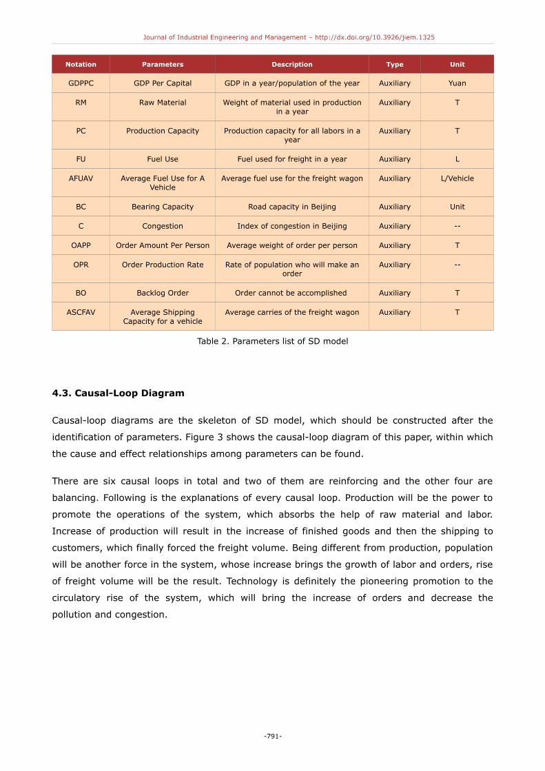
4.2. Identification of Parameters

Based on all the subsystems, key performance indicators can be put forward as Table 2

illustrated. Parameters are composed of stocks, flows and auxiliaries, which are clearly shown

in Table 2 with their notations, descriptions, types and units. Parameter of Freight Volume is

the representative of Beijing’s logistics demand, while CO2 Emission will explain the effect of

production and logistics to environment. At the same time, parameter of Average Shipping

Capacity for A Vehicle will tell the influence of logistics technology and Bearing Capacity

illustrates the competition between congestion and the increase of vehicles. To tackle with

some dilemmas, the government has proposed some important policies to decrease

-789-


congestions and environment pollution in Beijing. Based on all the parameters, we can do

some analysis and tests on the policies by changing the value of some important parameters,

which will be presented in Section 5.

Notation Parameters Description Type Unit

L Labor Total amount of labor of production inBeijing

Stock Million persons

Po Population Total population in Beijing Stock Million persons

GDP GDP The amount of annual GDP of Beijing Stock 10 million Yuan

OA Orders accomplished Total weight of accomplished orders inBeijing

Stock T

FGI Finished Goods Inventory Total weight of goods inventory inBeijing

Stock T

CE CO2 emission Total amount of CO2 emitted Stock Cubic meter

VA Vehicle amount The amount of freight wagons inBeijing

Stock Unit

FV Freight volume Total weight of annual freight in Beijing Stock T

LI Labor Increase Total amount of labor of productionincreased in Being during one year

Flow Millionpersons/year

PI Population Increase Total population increased in Beijingduring one year

Flow Millionpersons/year

GDPI GDP Increase The amount of annual GDP increase inBeijing

Flow 10 millionYuan/year

Pr1 Production Total weight produced in Beijing in oneyear

Flow T/year

S Sales Total weight sold in Beijing in one year Flow T/year

OP Order Production Total weight ordered in Beijing in oneyear

Flow T/year

VAI Vehicle Amount Increase The amount of freight wagon increasedin Beijing during one year

Flow Unit/year

VAD Vehicle Amount Decrease The amount of freight wagondecreased in Beijing during one year

Flow Unit/year

FVI Freight Volume Increase Freight increased in Beijing during oneyear

Flow T/year

FVD Freight Volume Decrease Freight decreased in Beijing during oneyear

Flow T/year

LIR Labor Increase Rate Labor in production increased rateevery year

Auxiliary --

Pr2 Productivity Productivity of per labor Auxiliary T

PIF Population IncreaseFraction

Population increased rate every year Auxiliary --

GDPIR GDP Increase Rate GDP increased rate every year Auxiliary --

-790-


Notation Parameters Description Type Unit

GDPPC GDP Per Capital GDP in a year/population of the year Auxiliary Yuan

RM Raw Material Weight of material used in productionin a year

Auxiliary T

PC Production Capacity Production capacity for all labors in ayear

Auxiliary T

FU Fuel Use Fuel used for freight in a year Auxiliary L

AFUAV Average Fuel Use for AVehicle

Average fuel use for the freight wagon Auxiliary L/Vehicle

BC Bearing Capacity Road capacity in Beijing Auxiliary Unit

C Congestion Index of congestion in Beijing Auxiliary --

OAPP Order Amount Per Person Average weight of order per person Auxiliary T

OPR Order Production Rate Rate of population who will make anorder

Auxiliary --

BO Backlog Order Order cannot be accomplished Auxiliary T

ASCFAV Average ShippingCapacity for a vehicle

Average carries of the freight wagon Auxiliary T

Table 2. Parameters list of SD model

4.3. Causal-Loop Diagram

Causal-loop diagrams are the skeleton of SD model, which should be constructed after the

identification of parameters. Figure 3 shows the causal-loop diagram of this paper, within which

the cause and effect relationships among parameters can be found.

There are six causal loops in total and two of them are reinforcing and the other four are

balancing. Following is the explanations of every causal loop. Production will be the power to

promote the operations of the system, which absorbs the help of raw material and labor.

Increase of production will result in the increase of finished goods and then the shipping to

customers, which finally forced the freight volume. Being different from production, population

will be another force in the system, whose increase brings the growth of labor and orders, rise

of freight volume will be the result. Technology is definitely the pioneering promotion to the

circulatory rise of the system, which will bring the increase of orders and decrease the

pollution and congestion.

-791-


Figure 3. Causal loop diagram of SD model

(1) Finished inventory → shipping to customer → Finished inventory (Balancing-1)

(2) Order production → Freight volume → GDP → Order production (Reinforcing-1)

(3) Order production → Freight volume → GDP → Technology → order production (Reinforcing-

2)

(4) Vehicles amount → Pollution → Vehicles amount (Balancing-2)

(5) Vehicles amount → Congestion → Vehicles amount (Balancing-3)

(6) Production → Shipping to customer → Freight volume → GDP → Technology → Population

→ Labor → Production (Balancing-4)

4.4. Stock and Flow Diagrams

Stock and flow diagram is the algebraic representation of model based on the causal loops

identified (Egilmez and Tatari, 2012). In this section, stock and flow diagram is shown as

Figure 4. In SD model, stocks can be calculated with the integration of their flows, whose

structure is presented in (1) as an integration equation. Stocks will be first defined and then

are the flows and auxiliaries.

(1)

Following is the separate explanations for some key variables.

-792-


• Labor (L): Labor is a stock parameter, which will be calculated as follows:

(2)

(3)

Where LIR will be decided by the change of Population Increase Fraction (PIF), which

will be calculated by the multiplication of the PIF and a proper factor.

• Population(P):

(4)

(5)

Where PIF is calculate by a lookup function with data from Beijing’s annual statistical

book.

• GDP:

(6)

Where GDPI is the GDP increase every year calculated as (7), the GDP Increase Rate

(GDPIR) is calculated by a lookup function with data from Beijing’s annual statistical

book.

(7)

• Finished Goods Inventory (FGI):

(8)

Parameter Pr1 will be affected by two other indexes of RM and PC, the minimum value

between the two parameters will decide the value of Pr1, whose calculation will be

(9)

a is a changeable factor that means a transfer rate from raw material to finished

products. RM is assumed as a constant variable and PC is calculated as:

(10)

-793-


• Orders Accomplished (OA):

(11)

As the model structured, OP is assume the same as S, which is affected by parameters

of OAPP, GDPPC, P and OPR, will be calculated as

(12)

• CO2 Emission

CE will arise by procedure of production and the fuel use for freight, whose calculation

is

(13)

b and g is the rate of CO2 from production and fuel use for freight.

(14)

AFU is treated as a constant variable.

CE is related to congestions in cities. People have to use less vehicles if CO2 emission is

very high, what helps decrease congestion coincidentally. So, the calculation for

Congestion (C) is:

(15)

Bearing Capacity (BC) represents the total amount of vehicles could be drive on the

road, which is assumed as a constant number since there are not so many spaces for

Beijing to the road construction.

• Vehicle Amount (VA):

(16)

(17)

Where the S is the same as P and the ASCAV is a constant variable.

(18)

-794-


• Freight Volume (FV):

FV is treated as the representative of logistics demand in this paper, whose calculation

is:

(19)

(20)

(21)

Figure 4. Stock and flow diagram of SD model

5. Policy Analysis

As the political center of China, Beijing is the city where most of the key policies are put

forward. With the speeding up expansion of the capital, Beijing is faced with more and more

problems, which forced Beijing’s government to issue some powerful measures and polices.

Some of the policies were closely related to Beijing’s logistics system.

Promotion of logistics technology, especially some technologies to increase logistics efficiency

and decrease the pollution to environment.

Ways to enhancing the bearing capacity of Beijing city, no matter the by the way of

construction or by the way of management.

Based on the structured SD model, we will try to verify the policies with the simulations.

-795-


5.1. Promotion of Logistics Technology

In this paper, parameter of ASCAV is treated as the representative of logistics technology,

which means that if the average shipping capacity of a vehicle increased, then we thought that

logistics technology developed.

5.1.1. Enhance the Average Shipping Capacity of a Vehicle

To verify this kind of policy, this paper selected the parameter of ASCAV. The initial value of

ASCAV is 0, which was set as 40t, 80t, 120t and represented with a green line, a red line and a

blue line separately. And we got pictures as shown in Figure 5, 6 and 7. In Figure 5, FV doesn’t

present any difference when the ASCAV changes, which means this kind of technology is not

the force of Beijing’s logistics demand. But we do find some changes in Figure 6 and Figure 7,

in which the amount of vehicle and CO2 emission show a downward trend with the increase of

ASCAV. The experiment results give three enlightenments to us:

• Technology on improving freight facilities won’t stimulate demand, which means if the

government wants to obtain an increasing logistics demand, some other kinds of

technology like e-commerce or rush delivery may be proposed.

• Bigger wagons can bring less vehicle amount.

• Bigger wagons can bring less CO2 emission.

• Recently, vehicles with yellow license plate are forbidden to appear inside the Fifth Ring

Road during the day time to ensure the safe of the city and unimpeded traffic, which

means all the freight wagons couldn’t come into the city center unless the goods in

freight wagons are changed into little vans with blue license plate. The result of this

phenomenon is the increase of vehicles and against with the experiment results based

on SD model, which will finally lead to higher CO2 emission. Beijing government has no

choice to put forward with the forbidden policy, though the consequence will do harm to

efficiency and environment.

-796-


Figure 5. Experiment for freight volume with changes of ASCAV

Figure 6. Experiment for vehicle amount with changes of ASCAV

-797-


Figure 7. Experiment for CO2 emission with changes of ASCAV

5.1.2. Reduce Average Fuel Use for a Vehicle

Beijing government has issued some policies to vehicle users for the decrease of average fuel

use for a vehicle, which won’t bring a directly change of logistics demand either, but will be

beneficial to environment protection. AFUAV is an auxiliary in SD model, which is regarded as

the representative of technology, especially for protect environment from being polluted from

freight. So AFUAV is designed as 5000, 10000, 15000 and illustrated with a green line, red line

and blue line. The result of experiment tells that with the decreasing fuel use CO2 emission and

the rate of the increase of the emission will go down.

Figure 8. Experiment for CO2 emission with changes of AFUAV

-798-


Based on the above experiments and analysis, we make sure that ASCAV and AFUAV won’t

bring a change to freight volume directly, though the benefit to social and environment is

obvious. But on the other side, decrease of vehicle amount can help with the reduction of

congestion, which could bring a better traffic condition for urban logistics. If the CO2 emission

keeps going on, it is definitely that government will force people to reduce the holding volume

of vehicles, which will make many orders delay and reduce urban logistics demand mediately.

5.2. Ways to Enhance the Bearing Capacity

Parameter of BC represents the bearing capacity of the road in Beijing. The limit of bearing

capacity in Beijing has been broken through since the booming of population and vehicles.

Heavy congestions are everywhere in Beijing, which lead to delay of freight and decrease of

logistics demand mediately. We assume the value of BC as 200, 500, 800 and illustrated the

changes of congestions with green line, red line and blue line, shown as Figure 9. The

experiment result shows that with the increase of a cities bearing capacity, congestion will be

greatly decreased.

Figure 9. Experiment for CO2 emission with changes of BC

-799-


Actually, congestions usually appear in the center and main road of Beijing, where no space

can be used for construction. These years the government put forward with some other

policies to enhance the bearing capacity:

• Time limited-entry policy.

• Wagon limited-entry policy

• Limited –entry policy to vehicles authorized in other provinces

• Better traffic management

• Constructions for subways

6. Conclusion

Due to complicated characteristics of urban logistics and sophisticated relations with other

systems, the simulation for urban logistics demand is definitely a systematic work, which

contains not only the conditions of urban logistics demand itself, but also requires a large

amount of work studying on some other related factors like society, population, economy,

environment and etc. Based on that, SD methodology is an excellent tool with a systematic

thought, which can help us figure out the relationships of numerous variables and find out the

variables’ changing direction.

This paper gave out a clear list of parameters representing the key performances of Beijing’s

logistics system. Based on those parameters, causal loop diagram and stock and flow diagram

were constructed. With the tested SD model, we realized some experiments by changing some

of the auxiliaries in SD model. We found that: (1) technologies like enhancing the average

shipping capacity for a vehicle and decreasing the average fuel use for a vehicle will not bring a

direct change of logistics demand in Beijing. Some forbidden policies issued by Beijing

government will do aggravate congestion and environment pollution; (2) ways to enhance the

bearing capacity will decrease the CO2 emission directly and promote logistics demand

mediately. Some limited policies authorized by Beijing government is helpful to decrease

congestions and CO2 emission, and will help with the increase of Beijing’s logistics demand.

Acknowledgements

This work is supported by Natural Science Foundation of China (Grant No. 713900334),

"EC-China Research Network on Integrated Container Supply Chains" Project (Grant

NO.612546)", Program for New Century Excellent Talents in University (Grant No.

NCET-11-0567) and funded by the Lab of Logistics Management and Technology.

-800-


References

Ansari, N., & Seifi, A. (2013). A system dynamics model for analyzing energy consumption and

CO2 emission in Iranian cement industry under various production and export scenarios.

Energy Policy, 58, 75-89. http://dx.doi.org/10.1016/j.enpol.2013.02.042

Bockermann, A., Meyer, B., Omann, I., & Spangenberg, J.H. (2005). Modelling sustainability

comparing an econometric (PANTA RHEI) and a systems dynamics model (SuE). Journal of

Policy Modeling, 27(2), 189-210. http://dx.doi.org/10.1016/j.jpolmod.2004.11.002

Bouloiz, H., Garbolino, E., Tkiouat, M., & Guarnieri, F. (2013). A system dynamics model for

behavioral analysis of safety conditions in a chemical storage unit. Safety Science, 58, 32-40.http://dx.doi.org/10.1016/j.ssci.2013.02.013

Cai, L. (2008).The application of system dynamics in the research of sustainable development.

Beijing: China Environmental Science Press.

Collins, R.D., Neufville, R., Claro, J., Oliveira, T., & Pacheco, A.P. (2013). Forest fire

management to avoid unintended consequences: A case study of Portugal using system

dynamics. Journal of Environmental Management, 130(30), 1-9.

http://dx.doi.org/10.1016/j.jenvman.2013.08.033

Egilmez, G., & Tatari, O. (2012). A dynamic modeling approach to highway sustainability:

Strategies to reduce overall impact. Transportation Research Part A, 46(7), 1086-1096.http://dx.doi.org/10.1016/j.tra.2012.04.011

Faezipour, M., & Ferreira, S. (2013). A system dynamics perspective of patient satisfaction in

healthcare. Procedia Computer Science, 16, 148-156. http://dx.doi.org/10.1016/j.procs.2013.01.016

Forrester, J.W. (1961). Industrial dynamics. MIT Press

Forrester, J.W. (1968). Principles of Systems. MIT Press

Forrester, J.W. (1969). Urban dynamics. MIT Press

Forrester, J.W. (1971). World dynamics. Wright-Allen Press

Georgiadis, P. (2013). An integrated System Dynamics model for strategic capacity planning in

closed-loop recycling networks: A dynamic analysis for the paper industry. Simulation

Modeling Practice and Theory, 32, 116-137. http://dx.doi.org/10.1016/j.simpat.2012.11.009

Georgiadis, P., Vlachos, D. & Iakovou, E. (2005). A system dynamics modeling framework for

the strategic supply chain management of food chains. Journal of Food Engineering, 70(3),

351-364. http://dx.doi.org/10.1016/j.jfoodeng.2004.06.030

-801-

http://dx.doi.org/10.1016/j.jfoodeng.2004.06.030

http://dx.doi.org/10.1016/j.simpat.2012.11.009

http://dx.doi.org/10.1016/j.procs.2013.01.016

http://dx.doi.org/10.1016/j.tra.2012.04.011

http://dx.doi.org/10.1016/j.jenvman.2013.08.033

http://dx.doi.org/10.1016/j.ssci.2013.02.013

http://dx.doi.org/10.1016/j.jpolmod.2004.11.002

http://dx.doi.org/10.1016/j.enpol.2013.02.042


Georgiadis, P., & Besiou, M. (2008). Sustainability in electrical and electronic equipment

closed-loop supply chains: A system dynamics approach. Journal of Cleaner Production,

16(15), 1665-1678. http://dx.doi.org/10.1016/j.jclepro.2008.04.019

Ghazvini, A., & Shukur, Z. (2013). System Dynamics in E-Health Policy Making and the “Glocal”

Concept. Procedia Technology, 11, 155-160. http://dx.doi.org/10.1016/j.protcy.2013.12.175

Jin, W., Xu, L., & Yang, Z. (2009). Modelling a policy making framework for urban

sustainability: Incorporating system dynamics into the Ecological Footprint. Ecological

Economics, 68(12), 2938-2949. http://dx.doi.org/10.1016/j.ecolecon.2009.06.010

Mavrommati, G., Bithas, K., & Panayiotidis, P. (2013). Operationalizing sustainability in urban

coastal systems: A system dynamics analysis. Water Research, 17(20), 7235-7250.http://dx.doi.org/10.1016/j.watres.2013.10.041

Meadows, D.H., Meadows, D.L., Randers, J., & Behrens, W. (1972). The limits to growth.

Universe Books

Musango, J.K., Brent, A.C., Amigun, B., Pretorius, L., & Muller, H. (2012). A system dynamics

approach to technology sustainability assessment: The case of biodiesel developments in

South Africa. Technovation, 32(11), 639-651. http://dx.doi.org/10.1016/j.technovation.2012.06.003

Poles, R. (2013). System Dynamics modelling of a production and inventory system for

remanufacturing to evaluate system improvement strategies. Int J Production Economics,

144(1), 189-199. http://dx.doi.org/10.1016/j.ijpe.2013.02.003

Qudrat-Ullah, H. (2013). Understanding the dynamics of electricity generation capacity in

Canada: A system dynamics approach. Energy, 59(15), 285-294.

http://dx.doi.org/10.1016/j.energy.2013.07.029

Rasjidin, R., Kumar, A., Alam, F., & Abosuliman, S. (2012). A system dynamics conceptual

model on retail electricity supply and demand system to minimize retailer’s cost in eastern

Australia. Procedia Engineering, 49, 330-337. http://dx.doi.org/10.1016/j.proeng.2012.10.145

Shouping, G., Qiang, Z., & Lifang, L. (2005). Area Logistics System Based on System Dynamics

Model. Tsinghua Science and Technology, 10(2), 265-269. http://dx.doi.org/10.1016/S1007-

0214(05)70065-1

Tako, A.A., & Robinson, S. (2012). The application of discrete event simulation and system

dynamics in the logistics and supply chain context. Decision Support Systems, 52(4), 802-

815. http://dx.doi.org/10.1016/j.dss.2011.11.015

-802-

http://dx.doi.org/10.1016/j.dss.2011.11.015

http://dx.doi.org/10.1016/S1007-0214(05)70065-1

http://dx.doi.org/10.1016/S1007-0214(05)70065-1

http://dx.doi.org/10.1016/j.proeng.2012.10.145

http://dx.doi.org/10.1016/j.energy.2013.07.029

http://dx.doi.org/10.1016/j.ijpe.2013.02.003

http://dx.doi.org/10.1016/j.technovation.2012.06.003

http://dx.doi.org/10.1016/j.watres.2013.10.041

http://dx.doi.org/10.1016/j.ecolecon.2009.06.010

http://dx.doi.org/10.1016/j.protcy.2013.12.175

http://dx.doi.org/10.1016/j.jclepro.2008.04.019


Teimoury, E., Nedaei, H., Ansari, S., & Sabbaghi, M. (2013). A multi-objective analysis for

import quota policy making in a perishable fruit and vegetable supply chain: A system

dynamics approach. Computers and Electronics in Agriculture, 93, 37-45.

http://dx.doi.org/10.1016/j.compag.2013.01.010

Tong, L., & Dou, Y. (2014). Simulation study of coal mine safety investment based on system

dynamics. International Journal of Mining Science and Technonogy, 24(2), 201-205.http://dx.doi.org/10.1016/j.ijmst.2014.01.010

Xu, Z., & Coors, V. (2012). Combining system dynamics model, GIS and 3D visualization in

sustainability assessment of urban residential development. Building and Environment, 47,

272-287. http://dx.doi.org/10.1016/j.buildenv.2011.07.012

Zaim, S., Bayyurt, N., Tarim, M., Zaim, H., & Guc, Y. (2013). System dynamics modeling of a

knowledge management process: A case study in Turkish Airlines. Procedia Social and

Behavioral Sciences, 99(6), 545-552. http://dx.doi.org/10.1016/j.sbspro.2013.10.524

Zhong, Y., Jia, X, & Qian, Y. (2013). System Dynamics. Beijing: Science Press.

Journal of Industrial Engineering and Management, 2015 (www.jiem.org)

Article's contents are provided on a Attribution-Non Commercial 3.0 Creative commons license. Readers are allowed to copy, distribute

and communicate article's contents, provided the author's and Journal of Industrial Engineering and Management's names are included.

It must not be used for commercial purposes. To see the complete license contents, please visit

http://creativecommons.org/licenses/by-nc/3.0/.

-803-

http://www.intangiblecapital.org/




http://dx.doi.org/10.1016/j.sbspro.2013.10.524

http://dx.doi.org/10.1016/j.buildenv.2011.07.012

http://dx.doi.org/10.1016/j.ijmst.2014.01.010

http://dx.doi.org/10.1016/j.compag.2013.01.010

a system dynamics model for simulating the logistics demand

Documents