a system of linear equations is a set of linear equations ...d00922011/matlab/282/20170624.pdf ·...

System of Linear Equations

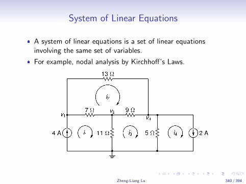
� A system of linear equations is a set of linear equationsinvolving the same set of variables.

� For example, nodal analysis by Kirchhoff’s Laws.

Zheng-Liang Lu 340 / 394

� A general system of m linear equations with n unknowns canbe written as

a11x1 +a12x2 · · · +a1nxn = b1a21x1 +a22x2 · · · +a2nxn = b2

......

. . .... =

...am1x1 +am2x2 · · · +amnxn = bm

where x1, . . . , xn are unknowns, a11, . . . , amn are thecoefficients of the system, and b1, . . . , bm are the constantterms.


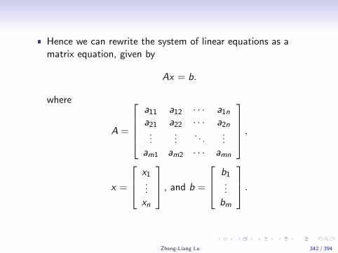
� Hence we can rewrite the system of linear equations as amatrix equation, given by

Ax = b.

where

A =

a11 a12 · · · a1na21 a22 · · · a2n

......

. . ....

am1 am2 · · · amn

,

x =

x1...xn

, and b =

b1...bm

.


Solving General System of Linear Equations

� Let x be the column vector with n independent variables andm constraints.1

� If m = n, then there exists the unique solution.2

� If m > n, then there is no exact solution.� Fortunately, we can find a least-squares error solution such

that ‖Ax ′ − b‖2 is minimal. (See the next page.)

� If m < n, then there are infinitely many solutions.

� We can calculate the inverse by simply using the left matrixdivide operator (\) or mldivide like this:

x = A\b.

1Assume that they are linearly independent.2Equivalently, rank(A) = rank([A, b]). Also see Cramer’s rule.


https://en.wikipedia.org/wiki/Cramer's_rule

Unique Solution (m = n)

� For example, 3x +2y −z = 1x −y +2z = −1−2x +y −2z = 0

1 >> A = [3 2 -1; 1 -1 2; -2 1 -2];2 >> b = [1; -1; 0];3 >> x = A \ b4

5 16 -27 -2


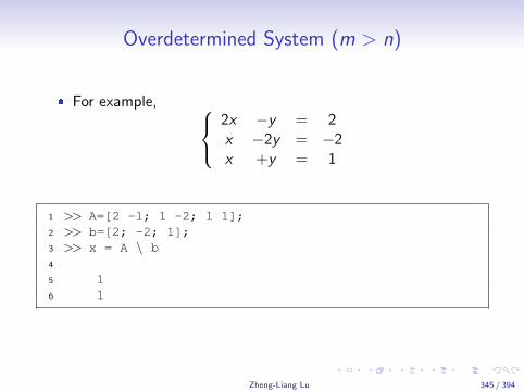
Overdetermined System (m > n)

� For example, 2x −y = 2x −2y = −2x +y = 1

1 >> A=[2 -1; 1 -2; 1 1];2 >> b=[2; -2; 1];3 >> x = A \ b4

5 16 1


Underdetermined System (m < n)� For example, {

x +2y +3z = 74x +5y +6z = 8

1 >> A = [1 2 3; 4 5 6];2 >> b = [7; 8];3 >> x = A \ b4

5 -36 07 3.3338

9 % (Why?)

� Note that this solution is a basic solution, one of infinitelymany.

� How to find the directional vector?Zheng-Liang Lu 346 / 394

Gaussian Elimination

� Recall the procedure of Gaussian Elimination in high school.

� Now we proceed to write a program which solves the followingsimultaneous equations:

3x +2y −z = 1x −y +2z = −1

−2x +y −2z = 0

� Then we have x = 1, y = −2, and z = −2.


� Suppose det(A) 6= 0.

� Form an upper triangular matrix

A =

1 a12 · · · a1n0 1 · · · a2n...

... 1...

0 0 · · · 1

with b =

b1b2...bn

,where aijs and bi s are the values after math.

� Use a backward substitution to determine the solution vectorx by

xi = bi −n∑

j=i+1

aijxj ,

where i = 1, 2, · · · , n.


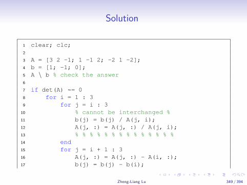
Solution

1 clear; clc;2

3 A = [3 2 -1; 1 -1 2; -2 1 -2];4 b = [1; -1; 0];5 A \ b % check the answer6

7 if det(A) ~= 08 for i = 1 : 39 for j = i : 3

10 % cannot be interchanged %11 b(j) = b(j) / A(j, i);12 A(j, :) = A(j, :) / A(j, i);13 % % % % % % % % % % % % % %14 end15 for j = i + 1 : 316 A(j, :) = A(j, :) - A(i, :);17 b(j) = b(j) - b(i);


18 end19 end20 x = zeros(3, 1);21 for i = 3 : -1 : 122 x(i) = b(i);23 for j = i + 1 : 1 : 324 x(i) = x(i) - A(i, j) * x(j);25 end26 end27 else28 disp('No unique solution.');29 end30 x


Exercise

� Write a program which solves a general system of linearequations.

� The function rank(A) provides an estimate of the number oflinearly independent rows or columns of A.3

� Check if rank(A) = rank([A, b]).� If so, then there is at least one solution.� If not, then there is no solution.

� The function rref([A, b]) produces the reduced row echelonform of A.

3rank(A) ≤ min{r , c} where r and c are the numbers of rows and columns.Zheng-Liang Lu 351 / 394

Solution

1 function y = linearSolver(A, b)2

3 if rank(A) == rank([A, b]) % argumented matrix4 if rank(A) == size(A, 2);5 disp('Exact one solution.')6 x = A \ b7 else8 disp('Infinite numbers of solutions.')9 rref([A b])

10 end11 else12 disp('There is no solution. (Only least ...

square solutions.)')13 end


Example: 2D Laplace’s Equation for Electrostatics

� Laplace’s equation4 is one of 2nd-order partial differentialequations (PDEs).5

� Let Φ(x , y) be an electrical potential, which is a function ofx , y ∈ R.

� Consider∇2Φ(x , y) = 0,

where ∇2 = ∂2

∂x2+ ∂2

∂y2 is the Laplace operator.

� Solving Laplace’s equation in practical applications oftenrequires numerical methods.

4Pierre-Simon Laplace (1749–1827).5See

https://en.wikipedia.org/wiki/Partial_differential_equation.Zheng-Liang Lu 354 / 394

https://en.wikipedia.org/wiki/Partial_differential_equation

Rectangular Trough


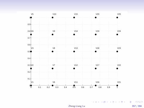
Extremely Simple Assumption

� First, we can partition the region into many subregions by aproper mesh generation.

� If Φ(x , y) satisfies the Laplace’s equation, then Φ(x , y) can beapproximated by

Φ(x , y) ≈ Φ(x + ε, y) + Φ(x − ε, y) + Φ(x , y + ε) + Φ(x , y − ε)4

,

where ε is a small distance compared with the system size.


0 0.1 0.2 0.3 0.4 0.5 0.6 0.7 0.8 0.9 10

0.1

0.2

0.3

0.4

0.5

0.6

0.7

0.8

0.9

1

V1

V2

V3

V4

V5

V6

V7

V8

V9

V10

V11

V12

V13

V14

V15

V16

V17

V18

V19

V20

V21

V22

V23

V24

V25


Reformulation

� Consider the boundary condition:� V1 = V2 = · · · = V4 = 0� V21 = V22 = · · · = V24 = 0� V1 = V6 = · · · = V16 = 0� V5 = V10 = · · · = V25 = 100

� Now define

x =[V7 V8 V9 V12 V13 V14 V17 V18 V19

]Twhere T is the transposition operator.


� Then we form Ax = b where

A =

4 −1 0 −1 0 0 0 0 0−1 4 −1 0 −1 0 0 0 00 −1 4 0 0 −1 0 0 0−1 0 0 4 −1 0 −1 0 00 −1 0 −1 4 −1 0 −1 00 0 −1 0 −1 4 −1 0 −10 0 0 −1 0 0 4 −1 00 0 0 0 −1 0 −1 4 −10 0 0 0 0 −1 0 −1 4

and

b =[

0 0 100 0 0 100 0 0 100]T.

� As you can see that V7 = V17,V8 = V18 and V9 = V19 due tothe spatial symmetry, the dimension of A can be reduced to 6!(Try.)


1 clear; clc; close all;2

3 a = 1; b = 1; n = 5; V0 = 100;4

5 x = linspace(0, a, 5);6 y = linspace(0, b, 5);7 [X Y] = meshgrid(x, y);8

9 figure; hold on; grid on;10 plot(X, Y, 'k.', 'markersize', 24);11 for i = 1 : length(x)12 for j = 1 : length(y)13 text(X(n * (i - 1) + j), Y(n * (i - 1) + ...

j) + 0.05, sprintf('V%d', n * (i - 1) ...+ j));

14 end15 end16

17 % boundary condition


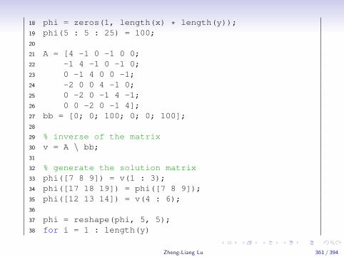
18 phi = zeros(1, length(x) * length(y));19 phi(5 : 5 : 25) = 100;20

21 A = [4 -1 0 -1 0 0;22 -1 4 -1 0 -1 0;23 0 -1 4 0 0 -1;24 -2 0 0 4 -1 0;25 0 -2 0 -1 4 -1;26 0 0 -2 0 -1 4];27 bb = [0; 0; 100; 0; 0; 100];28

29 % inverse of the matrix30 v = A \ bb;31

32 % generate the solution matrix33 phi([7 8 9]) = v(1 : 3);34 phi([17 18 19]) = phi([7 8 9]);35 phi([12 13 14]) = v(4 : 6);36

37 phi = reshape(phi, 5, 5);38 for i = 1 : length(y)


39 for j = 1 : length(x)40 h = text(X(n * (i - 1) + j), Y(n * (i - ...

1) + j) - 0.05, sprintf('%7.4f', ...phi(j, i)));

41 set(h, 'color', 'r');42 end43 end44

45 figure; hold on; grid on;46 contour(X, Y, phi); colorbar;

� This is a toy example for numerical methods.

� You may consider Finite Difference Method (FDM) and FiniteElement Method (FEM), both widely used in commercialsimulation softwares!6

� Besides, the mesh generation is also important for numericalmethods.7

6Read http://www.macs.hw.ac.uk/~ms713/lecture_1.pdf.7See https://en.wikipedia.org/wiki/Mesh_generation.


http://www.macs.hw.ac.uk/~ms713/lecture_1.pdf

https://en.wikipedia.org/wiki/Mesh_generation

0 0.1 0.2 0.3 0.4 0.5 0.6 0.7 0.8 0.9 10

0.1

0.2

0.3

0.4

0.5

0.6

0.7

0.8

0.9

1

10

1010

10

10

20

20

20

2030

3030

3040

40 40

4050

50 50

5060

60 60

70

70 70

80 8080

90 9090

100 100 100

10

20

30

40

50

60

70

80

90

100


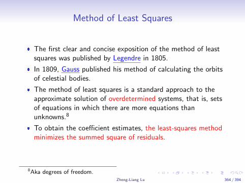
Method of Least Squares

� The first clear and concise exposition of the method of leastsquares was published by Legendre in 1805.

� In 1809, Gauss published his method of calculating the orbitsof celestial bodies.

� The method of least squares is a standard approach to theapproximate solution of overdetermined systems, that is, setsof equations in which there are more equations thanunknowns.8

� To obtain the coefficient estimates, the least-squares methodminimizes the summed square of residuals.

8Aka degrees of freedom.Zheng-Liang Lu 364 / 394

http://en.wikipedia.org/wiki/Adrien-Marie_Legendre

http://en.wikipedia.org/wiki/Carl_Friedrich_Gauss

� Let {yi}ni=1 be the observed response values and {yi}ni=1 bethe fitted response values.

� Let εi = yi − yi be the residual for i = 1, . . . , n.

� Then the sum of square error estimates associated with thedata is given by

S =n∑

i=1

ε2i .


Illustration


Linear Least Squares

� In the sense of linear least squares, a linear model is said to bean equation which is linear in the coefficients.

� Now we choose a linear equation,

y = ax + b,

where a and b are to be determined.

� So εi = (axi + b)− yi and then

S =n∑

i=1

((axi + b)− yi )2.

� The coefficient a and b can be determined by differentiating Swith respect to each parameter, and setting the result equalto zero. (Why?)


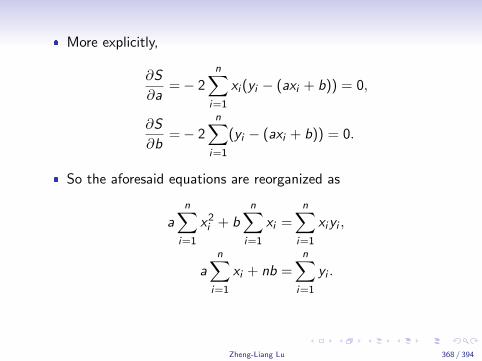
� More explicitly,

∂S

∂a=− 2

n∑i=1

xi (yi − (axi + b)) = 0,

∂S

∂b=− 2

n∑i=1

(yi − (axi + b)) = 0.

� So the aforesaid equations are reorganized as

an∑

i=1

x2i + bn∑

i=1

xi =n∑

i=1

xiyi ,

an∑

i=1

xi + nb =n∑

i=1

yi .


� In form of matrices,[ ∑ni=1 x

2i

∑ni=1 xi∑n

i=1 xi n

] [ab

]=

[ ∑ni=1 xiyi∑ni=1 yi

].

� So we have

a =n∑n

i=1 xiyi −∑n

i=1 xi∑n

i=1 yin∑n

i=1 x2i − (

∑ni=1 xi )

2=

cov(x , y)

cov(x),

where cov(x , y) denotes the covariance between x = {xi}ni=1

and y = {yi}ni=1.

� Then we have

b =1

n(

n∑i=1

yi − an∑

i=1

xi ).


Example: Circle Fitting

� Consider a set of data points surrounding some center.

� Now the coordinates of the circle center and also the radiusare desired.

� This needs to estimate 3 unknowns: (xc , yc) and r > 0.

� Recall that a circle equation is (x − xc)2 + (y − yc)2 = r2.

� The above equation can be equivalent to

2xxc + 2yyc + z = x2 + y2,

wherez = r2 − x2c + y2c .


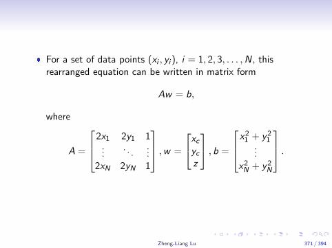
� For a set of data points (xi , yi ), i = 1, 2, 3, . . . ,N, thisrearranged equation can be written in matrix form

Aw = b,

where

A =

2x1 2y1 1...

. . ....

2xN 2yN 1

,w =

xcycz

, b =

x21 + y21

...x2N + y2N

.



3 N = 100;4 theta = 2 * pi * rand(1, N);5 xcc = 5;6 ycc = 3;7 rcc = 10;8

9 x = xcc + rcc * cos(theta) + randn(1, N) * 0.5;10 y = ycc + rcc * sin(theta) + randn(1, N) * 0.5;11

12 xt = x - mean(x);13 yt = y - mean(y);14 distance = sqrt(xt .ˆ 2 + yt .ˆ 2)15 maxR = max(distance);16

17 xt = xt / maxR;18 yt = yt / maxR;19 distance = distance / maxR;


20

21 A = [2 * xt', 2 * yt', ones(N, 1)];22 b = (distance .ˆ 2)';23

24 % v = [xc; yc; z]25 v = A \ b26 r = sqrt(v(3) + v(1) ˆ 2 + v(2) ˆ 2) * maxR27 xc = v(1) * maxR + mean(x)28 yc = v(2) * maxR + mean(y)29

30 figure; plot(x, y, 'o');31 hold on; grid on; axis equal;32

33 theta = linspace(0, 2 * pi, 100);34 x = xc + r * cos(theta );35 y = yc + r * sin(theta );36 plot(x , y , 'r-');


−5 0 5 10 15

−6

−4

−2

0

2

4

6

8

10

12


Polynomials9

� In fact, all polynomials of n-th order with addition andmultiplication to scalars form a vector space, denoted by Pn.

� In general, f (x) is said to be a polynomial of n-order providedthat

f (x) = anxn + an−1x

n−1 + · · ·+ a0,

where an 6= 0.

� It is convenient to express a polynomial by a coefficient vector(an, an−1, . . . , a0), where the elements are the coefficients ofthe polynomial in descending order.

9Weierstrass approximation theorem states that every continuous functiondefined on a closed interval [a, b] can be uniformly approximated as closely asdesired by a polynomial function. Seehttps://en.wikipedia.org/wiki/Stone_Weierstrass_theorem.


https://en.wikipedia.org/wiki/Stone_Weierstrass_theorem

Arithmetic Operations

� P1 + P2 returns the addition of two polynomials.

� P1 − P2 returns the subtraction of two polynomials.

� The function conv(P1,P2) returns the resulting coefficientvector for multiplication of the two polynomials P1 and P2.10

� The function [Q,R] = deconv(B,A) deconvolves vector Aout of vector B.

� Equivalently, B = conv(A,Q) + R.� This is so-called “Euclidean division algorithm.”

� The function polyval(P,X ) returns the values of a polynomialP evaluated at x ∈ X .

10See Convolution.Zheng-Liang Lu 376 / 394

http://en.wikipedia.org/wiki/Euclidean_division

http://en.wikipedia.org/wiki/Convolution

1 clear; clc;2

3 p1 = [1 -2 -7 4];4 p2 = [2 -1 0 6];5 %%% addition6 p3 = p1 + p27 %%% substraction8 p4 = p1 - p29 %%% multiplcaition

10 p5 = conv(p1, p2)11 %%% division: q is quotient and r is remainder12 [q, r] = deconv(p1, p2)13 x = -1 : 0.1 : 1;14 plot(x, polyval(p1, x), 'o', x, polyval(p2, x), ...

'*', x, polyval(p5, x), 'd');15 grid on; legend('p1', 'p2', 'conv(p1, p2)');


−1 −0.5 0 0.5 1

−20

−10

0

10

20

30

p1p2conv(p1,p2)


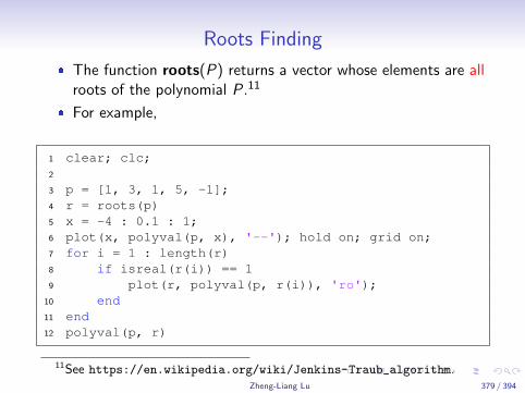
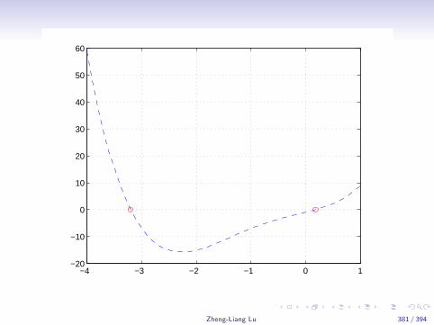
Roots Finding

� The function roots(P) returns a vector whose elements are allroots of the polynomial P.11

� For example,

1 clear; clc;2

3 p = [1, 3, 1, 5, -1];4 r = roots(p)5 x = -4 : 0.1 : 1;6 plot(x, polyval(p, x), '--'); hold on; grid on;7 for i = 1 : length(r)8 if isreal(r(i)) == 19 plot(r, polyval(p, r(i)), 'ro');

10 end11 end12 polyval(p, r)

11See https://en.wikipedia.org/wiki/Jenkins-Traub_algorithm.Zheng-Liang Lu 379 / 394

https://en.wikipedia.org/wiki/Jenkins-Traub_algorithm

1 >> r =2

3 -3.20514 0.0082 + 1.2862i5 0.0082 - 1.2862i6 0.18867

8 >> ans =9

10 1.0e-013 *11

12 0.404113 -0.0133 + 0.0529i14 -0.0133 - 0.0529i15 0

� Why not exactly zero?


−4 −3 −2 −1 0 1−20

−10

0

10

20

30

40

50

60


Exercise: Internal Rate of Return (IRR)

� Given a collection of pairs (time, cash flow) involved in aproject, the IRR is a rate of return when the net present valueis zero.

� Explicitly, the IRR can be calculated by solving

N∑n=0

Cn

(1 + r)n= 0,

where Cn is the cash flow at time n.

� For example, consider an investment may be given by thesequence of cash flows:

C0 = −123400,C1 = 36200,C2 = 54800,C3 = 48100.

� Then the IRR is 5.96%.


Forming Polynomials

� The function poly(V ), where V is a vector, returns a vectorwhose elements are the coefficients of the polynomial whoseroots are the elements of V .

� Simply put, the function roots and poly are inverse functionsof each other.


Example

1 clear; clc;2

3 v = [0.5 sqrt(2) 3];4 y = 1;5 for i = 1 : 36 y = conv(y, [1 -v(i)]);7 end8 y9

10 poly(v)


Integral and Derivative of Polynomials

� The function polyder(P) returns the derivative of thepolynomial whose coefficients are the elements of vector P indescending powers.

� The function polyint(P,K ) returns a polynomial representingthe integral of polynomial P, using a scalar constant ofintegration K .

1 clear; clc;2

3 p = [4 3 2 1];4 p der = polyder(p)5 p int = polyint(p, 0) % assume K = 0


Exercise

� Consider f (x) = 4x3 + 3x2 + 2x + 1 for x ∈ R.

� Determine the coefficients of its derivative f ′ and integrationF (x) =

∫ x0 f (t)dt.

� Do not use the built-in functions.


1 clear; clc;2

3 p = [4 3 2 1];4 K = 0;5 q1 = zeros(1, length(p));6 for i = 2 : length(p) - 17 q1(i) = p(i - 1) * (length(p) - (i - 1));8 end9 q1

10

11 q2 = zeros(1, length(p) + 1);12 q2(length(q2)) = K;13 for i = 1 : length(p)14 q2(i) = 1 / (length(p) - i + 1) * p(i);15 end16 q2


Curve Fitting by Polynomials

� The function polyfit(x , y , n) returns the coefficients for apolynomial p(x) of degree n that is a best fit (in aleast-squares sense) for the data in y .


Example


3 x = linspace(0, 1, 10);4 y = cos(rand(1, length(x)) * pi / 2) + x .ˆ 2;5 figure; hold on; grid on; plot(x, y, 'o');6

7 color = 'rgbck';8 x = linspace(0, 1, 100);9 for i = 1 : 5

10 p = polyfit(x, y, i);11 plot(x , polyval(p, x ), color(i));12 end13 p14

15 A = [x' .ˆ 5, x' .ˆ 4, x' .ˆ 3, x' .ˆ 2, x' .ˆ 1, ...ones(10, 1)];

16 b = y';17 pp = A \ b


Overfitting


Occam’s Razor

“Entities must not be multiplied beyond necessity.”– Duns Scotus

� In science, Occam’s razor is used as a heuristic to guidescientists in developing theoretical models rather than as anarbiter between published models.

� Among competing hypotheses, the one with the fewestassumptions should be selected.

� For example, Runge’s phenomenon is a problem of oscillationat the edges of an interval that occurs when using polynomialinterpolation with polynomials of high degree over a set ofequispaced interpolation points.12

12See https://en.wikipedia.org/wiki/Runge’s_phenomenon.Zheng-Liang Lu 391 / 394

https://en.wikipedia.org/wiki/Runge's_phenomenon

Eigenvalues and Eigenvectors13

� Let A be a square matrix.

� Then v is an eigenvector associated with the eigenvalue λ if

Av = λv .

� Equivalently,(A− λI )v = 0.

� For nontrivial vectors v , det(A− λI ) = 0.

� The above equation is the so-called characteristic polynomial,whose roots are actually eigenvalues!

� Use eig(A) to derive the eigenvalues associated witheigenvectors for the matrix A.

13See https://en.wikipedia.org/wiki/Eigenvalues_and_

eigenvectors#Applications.Zheng-Liang Lu 392 / 394

https://en.wikipedia.org/wiki/Eigenvalues_and_eigenvectors#Applications

https://en.wikipedia.org/wiki/Eigenvalues_and_eigenvectors#Applications

Singular Value Decomposition (SVD)14

� Let Am×n be a matrix.

� Then σ is called one singular value associated with thesingular vectors u ∈ Rm×1 and v ∈ Rn×1 for A provided that{

Av = σu,ATu = σv .

� We further have {AV = UΣ,ATU = VΣ,

where U and V are both unitary, and the diagonal terms in Σare σ’s, 0’s in off-diagonal terms.

� You may use the built-in function svd.

14Seehttps://www.mathworks.com/help/matlab/math/singular-values.html.


https://www.mathworks.com/help/matlab/math/singular-values.html

Example: Low-rank Approximation for Image Compression

� This idea originates from Principal Component Analysis(PCA).15

� Use svd to calculate the principal components of the inputimage.

� Then we can have an image extremely similar to the originone, but with a smaller image size by keeping the vectorsassociated with a few first largest of principal components.

15See https://www.cs.princeton.edu/picasso/mats/

PCA-Tutorial-Intuition_jp.pdf andhttp://setosa.io/ev/principal-component-analysis/.


https://www.cs.princeton.edu/picasso/mats/PCA-Tutorial-Intuition_jp.pdf

https://www.cs.princeton.edu/picasso/mats/PCA-Tutorial-Intuition_jp.pdf

http://setosa.io/ev/principal-component-analysis/

a system of linear equations is a set of linear equations ...d00922011/matlab/282/20170624.pdf ·...

Documents