a systematic procedure to study the influence of occupant behavior on building energy

A Systematic Procedure to Study the Influence of Occupant

Behavior on Building Energy Consumption

Zhun Yu1, Benjamin C. M. Fung

2, Fariborz Haghighat

1, Hiroshi Yoshino

3, Edward

Morofsky 4

1Department of Building, Civil and Environmental Engineering, Concordia University,

Montreal, Quebec, H3G 1M8, Canada 2Concordia Institute for Information Systems Engineering, Concordia University,

Montreal, Quebec, H3G 1M8, Canada 3Department of Architecture and Building Science, Tohoku University, Japan

4Real Property Branch, Public Works and Government Services Canada, Place du Portage III,

8B1, Gatineau, Québec, K1A 0S5 Canada

Abstract

Efforts have been devoted to the identification of the impacts of occupant behavior on

building energy consumption. Various factors influence building energy consumption

at the same time, leading to the lack of precision when identifying the individual

effects of occupant behavior. This paper reports the development of a new

methodology for examining the influences of occupant behavior on building energy

consumption; the method is based on a basic data mining technique (cluster analysis).

To deal with data inconsistencies, min-max normalization is performed as a data

preprocessing step before clustering. Grey relational grades, a measure of relevancy

between two factors, are used as weighted coefficients of different attributes in cluster

analysis. To demonstrate the applicability of the proposed method, the method was

applied to a set of residential buildings’ measurement data. The results show that the

method facilitates the evaluation of building energy-saving potential by improving the

behavior of building occupants, and provides multifaceted insights into building

energy end-use patterns associated with the occupant behavior. The results obtained

could help prioritize efforts at modification of occupant behavior in order to reduce

building energy consumption, and help improve modeling of occupant behavior in

numerical simulation.

Keywords: Occupant behavior; Building energy consumption; Data mining; Cluster

analysis; Grey relational analysis

1 Introduction

The identification of major determinants of building energy consumption, together

with a thorough understanding of the impacts of the identified determinants on energy

consumption patterns, could assist in achieving the goal of improving building energy

performance and reducing greenhouse gas emissions due to the building energy

consumption. In general, the factor influencing the total building energy consumption

can be divided into seven categories:

(1) Climate (e.g., outdoor air temperature, solar radiation, wind velocity, etc.),

(2) Building-related characteristics (e.g., type, area, orientation, etc.)

(3) User-related characteristics, except for social and economic factors (e.g., user

presence, etc.),

(4) Building services systems and operation (e.g., space cooling/heating, hot water

supplying, etc.),

(5) Building occupants’ behavior and activities,

(6) Social and economic factors (e.g., degree of education, energy cost, etc.), and

(7) Indoor environmental quality required.

Among these seven factors, social and economic factors will partly determine the

occupant attitude toward energy consumption, and building occupants will embody

such impact on their daily activities and behavior, thereby influencing building energy

consumption. At the same time, indoor environment quality could be regarded as

being basically decided by building occupants, thereby influencing building energy

consumption. In essence, these two categories of factors which represent occupants’

influences affect building energy consumption indirectly. Therefore, their influences

on building energy consumption are already contained within the effects of occupant

behavior, and there is no need to take them into consideration when identifying the

effects of influencing factors.

The separate and combined influences of the first four factors on building energy

consumption can be identified via simulation. With a variety of parameter settings,

current simulation software is robust in respect to simulating different situations based

upon these four factors. However, it is difficult to completely identify the influences

of occupant behavior and activities through simulation due to users’ behavior diversity

and complexity; current simulation tools can only imitate behavior patterns in a rigid

way. In recent years several models have been established to integrate the influence of

building occupant behavior into building simulation programs [1-4]. However, these

models focus only on typical activities such as the control of sun-shading devices,

while realistic building user-behavior patterns are more complicated.

A number of studies [5-7] suggest that, in order to obtain the full effects of user

behavior, one possible approach is to extract corresponding useful information from

real measured data, since such data already contains the full effects. For example, Yu

et al [7] proposed a decision tree method for building energy demand modeling, and

applied this method to the historical data on Japanese residential buildings. The

generated model has a flowchart-like tree structure, enabling users to quickly extract

useful information on the influence factors of building energy consumption. Such

model along with derived information could benefit the improvement of building

energy performance greatly. Generally, the previous studies on the effects of occupant

behavior can be divided into two categories. The first category focuses on the effects

of building user presence on building energy consumption. For example, Emery and

Kippenhan [8] reported a survey on the effects of occupant presence upon home

energy usage in four nearly identical houses. The four houses were divided into two

pairs, and the building envelope of one pair was constructed with improved thermal

resistance. One of each pair of houses was left unoccupied, while the other was

occupied by university student families. Researchers compared the first heating

season’s (1987–88) total energy consumption of the occupied and unoccupied houses

(i.e., the sum of heating, lighting, and appliances). They found that the presence of

occupants increased the total energy consumption of both occupied houses, and the

house with the improved building envelope had a smaller increase. The second

category focuses on the effects of actions occupants took to influence energy

consumption. For example, Ouyang and Hokao [9] investigated energy-saving

potential by improving user behavior in 124 households in China. In this study, these

houses were divided into two groups: one was educated to promote energy-conscious

behavior and put corresponding energy-saving measures into effect in July 2008,

while the other was required to keep behavior intact. Comparisons were made

between monthly household electricity uses in July 2007 and July 2008 for both

groups. Researchers found that, on the average, effective promotion of

energy-conscious behavior could reduce household electricity consumption by more

than 10%. Evidently, comparative analyses on measured data were conducted in these

studies to identify the effects of user behavior. However, the limitations of this method

are significant. First, apart from user behavior, the other four influencing factors also

contribute to the variation in building energy consumption simultaneously, while this

method is unable to adequately remove the effects of those four factors and identify

the influences of occupant behavior. Although in these studies some measures were

implemented to remove the impact of those factors, such as using nearly identical

housing characteristics and taking energy data in other years with similar climatic

conditions as a reference, the effects of these measures are questionable since even a

slight difference in some building parameters (e.g., heat loss coefficient) and weather

parameters (e.g., annual average outdoor air temperature) would result in remarkable

fluctuations in the building energy consumption. Second, in real building databases,

buildings are usually described by a mixture of variable types such as numerical

variable, categorical variable (e.g., residential building types are divided into detached

and apartment), and ordinal variable (e.g., buildings are rated as platinum, gold, and

silver). Such data of mixed variable types is difficult to process by statistical methods

that are normally utilized in comparative analyses. This also adds the difficulty of

distinguishing between building-related effects and user-related effects. Third, with

regard to comparative analyses, buildings are usually classified into different groups

to simplify research. Such classification is commonly based on building-related

parameters, such as floor area. For example, if building floor area ranges from 100 m2

to 400 m2, it can be replaced by small, medium, and large corresponding to the

intervals [100, 200], [200, 300], and [300, 400], respectively. Accordingly, all the

buildings are classified into three groups, i.e. small buildings, medium buildings, and

large buildings; and further study can be performed on each group. In this process, the

partition of building-related parameters is normally decided by considerations of

convenience and intuition. Why should 200 m2 and 300 m

2 be the interval between

each group? Hence, a more rational classification method for grouping buildings is

required.

Moreover, buildings are commonly represented by various typical parameters at the

same time, such as building age and floor area. All these parameters may be divided

into different levels, such as low and high, for simplicity. In order to perform a

comprehensive investigation, the sample size (i.e. number of buildings) necessary for

research should be determined by the combination of different levels of all parameters.

For example, suppose seven typical parameters are selected for representation and

each are stratified into 3 levels (e.g. small, medium, and large). In terms of

combinatorial theory, it can be calculated that at least 37

= 2187 buildings should be

investigated for comparison, which may be quite impractical.

The main purpose of this paper is to develop a methodology for identifying the effects

of occupant behavior on the building energy consumption through data analysis,

thereby evaluating the energy saving potential by improving user behavior and

providing deep insights into the building energy consumption patterns.

This paper is organized as follows: Section 2 introduces the proposed methodology.

Section 3 describes the results of applying this method to a set of field measurement

data and discusses the related work. Section 4 concludes the paper.

2 Methodology

A new methodology is proposed for examining the effects of occupant behavior on the

building energy consumption. Basically, it is realized by organizing similar buildings

among all the investigated buildings into various groups based on the four influencing

factors unrelated to user behavior, so that for each building in the same group the four

factors have similar effects on the building energy consumption. Accordingly, the

effects of occupant behavior on the building energy consumption can be identified

accurately in these groups. Further, provided there is a sufficient building sample size

and subject buildings have a large divergence in the four influencing factors, implying

that the full effects of the four factors in each group can be similar enough and the

energy consumption difference caused by them is comparatively small, energy

consumption difference between buildings in each group could be thought of as being

caused only by occupant behavior. It is obvious that the identification of building

groups is the most important element of this methodology. Such identification is

achieved mainly via cluster analysis.

2.1 Cluster analysis

Cluster analysis is the process of grouping the observations into classes or clusters so

that objects in the same cluster have high similarity, while objects in different clusters

have low similarity. Fig. 1 shows a clustering schema based on a hypothetical building

data table. It contains various energy-related variables such as outdoor air temperature

(T) and building heat loss coefficient (HLC).

Attribute 1

(T)...

Attribute m

(HLC)

Instance 1

…

Instance i

Instance j

...

Instance n

x x x

x x x

x x x

x x x

x x x

x x x

Cluster 1

Cluster w

... x x x

Instance

...

Figure 1. Clustering schema

The data table consists of m attributes and n instances. Each attribute represents a

variable and each instance denotes a building. All the instances are grouped into w

clusters. Accordingly, these w clusters are homogeneous internally and heterogeneous

between different clusters [10]. Such internal cohesion and external separation are

based upon the m attributes as well as their influences; it implies that these attributes

have the most similar holistic effects on the building energy performance of the same

cluster buildings, while the effects are significantly distinct for the buildings in

different clusters. Therefore, the separate effects of occupant behavior on the building

energy consumption can be identified more precisely based on cluster analysis and the

four influencing factors unrelated to the occupant behavior. Note that these four

influencing factors are represented by corresponding parameters selected from an

existing database.

Before conducting cluster analysis, some preprocessing steps are needed in order to

deal with the inconsistencies of different attributes. For example, most of the

energy-related attributes have their own units. Switching attribute units from one to

another may significantly change the attribute values, thereby impacting the quality

and accuracy of clusters. Therefore, data transformation techniques should be applied

in order to help avoid dependence on the selection of attribute units. Also, data

transformation can help prevent attributes with large ranges from outweighing those

with comparatively smaller ranges. At the same time, the contribution of different

attributes to the building energy consumption may differ considerably; thus, after data

normalization, each attribute should be associated with a weight that reflects its

significance. Grey relational analysis will be used to identify such weights. The

procedure of data transformation and grey relational analysis will be introduced in

Sections 2.2 and 2.3, respectively.

The dissimilarity between observations in the database is calculated using the distance

between them in the cluster analysis. In this study, the most popular distance measure,

Euclidean distance, is used [10]:

𝑑(𝑘, 𝑙) = √(𝑥𝑘1 − 𝑥𝑙1)2 + (𝑥𝑘2 − 𝑥𝑙2)2 + ⋯ + (𝑥𝑘𝑛 − 𝑥𝑙𝑛)2

where k = (xk1, xk2, …, xkn) and l = (xl1, xl2, …, xln) are buildings. xk1, …, xkn are n

parameters of k and xl1, …, xln are n parameters of l.

Commonly used clustering algorithms include K-means, K-medoids, and CLARANS

[10]. In this study, we employ the K-means, along with open-source data mining

software WEKA [11], to perform cluster analysis, due to its high efficiency and wide

applicability.

The K-means algorithm is one of the simplest partition methods to solve clustering

problem. Given a dataset (D) containing w objects, the K-means algorithm aims to

partition these w objects into k clusters with two restraints: 1) the center of each

cluster is the mean position of all objects in that cluster, 2) each object has been

assigned to the cluster with the closest center. This algorithm consists of given steps: 1)

Randomly select k observations from D as the initial cluster centers, 2) Calculate the

distance between each remaining observation and each initially chosen center, 3)

Assign each remaining observation to the cluster with the closest center, 4)

Recalculate the mean values, i.e., the cluster centers, of the new clusters, and 5)

Repeat Steps 2 to 4 until the algorithm converges, meaning that the cluster centers do

not change. It should be mentioned that K-means is quite sensitive to initial cluster

centers. Therefore, different values should be tried so as to obtain the minimum sum

of the distances within a cluster. At the same time, the number of clusters should be

specified in advance.

2.2 Data transformation

As mentioned previously, data transformation has been applied in order to deal with

the inconsistencies in measured dataset. Specifically, min-max normalization [10] is

performed to scale the values so that they fall within a predetermined range. The main

advantage of min-max normalization lies in its ability to reserve the relationships

between the initial data since it carries out a linear normalization. Assume that xmax

and xmin are the original maximum and minimum values of a numerical attribute. By

min-max normalization, a value, x, of this attribute can be transformed to x’ in the

new specified range [x’min, x’max] by calculating

𝑥′ =𝑥 − 𝑥𝑚𝑖𝑛

𝑥𝑚𝑎𝑥 − 𝑥𝑚𝑖𝑛

(𝑥′𝑚𝑎𝑥 − 𝑥′𝑚𝑖𝑛) + 𝑥′𝑚𝑖𝑛

In this study, the new range is defined as [0, 1].

For binary attributes, their two states, such as the operation states of room air

conditioners, i.e. [ON, OFF], can be transformed to [0, 1] or [1, 0] directly. The

decision to recode these two states to either [0, 1] or [1, 0] depends upon whether or

not there is a preferred positive value.

For multi-valued categorical attributes with an implicit order, it is often necessary to

rank their ordered states first, and then map the obtained range onto [0, 1] by

𝑥𝑖 ′ =𝑟𝑎𝑛𝑘𝑖 − 1

𝑟𝑎𝑛𝑘𝑚𝑎𝑥 − 1

where

x’: transformed value of each state

ranki: corresponding rank of each state

rankmax: maximum rank

For example, the four levels of certification in the Leadership in Energy and

Environmental Design (LEED) Green Building Rating System, i.e. [CERTIFIED,

SILVER, GOLD, PLATINUM], will be transformed to [0, 1/3, 2/3, 1] using the

aforementioned method.

2.3 Grey relational analysis

Based on geometrical mathematics, grey relational analysis (GRA) has been proposed

in order to find grey relational grades and a grey relational order (i.e. the rank of grey

relational grades) that can be used to describe primary trend relationships between

related factors, and to identify the important factors that significantly influence

predefined target factors [12]. For example, if the building energy consumption is

defined as the target factor, GRA can provide grey relational grades for its various

influencing factors, such as outdoor air temperature and floor area. These grey

relational grades are numerical measures of the impact of the influencing factors on

the total building energy consumption. The larger the grey relational grades are, the

more significant impacts the influencing factors have. In comparison with other

similar multi-factorial analysis methods such as regression analysis and principal

component analysis, the main advantages of GRA are its comparative simplicity and

the ability to deal with small data sets that do not have typical probability

distributions.

Let y0 be the objective sequence (measured data of target factor, such as the building

energy consumption) and yi be the compared sequences (measured data of related

factors, such as various influencing factors of building energy consumption):

𝑦0 = (𝑦0(1), y0(2), … , y0(𝑛))

y𝑖 = (y𝑖(1), y𝑖(2), … , y𝑖(𝑛)), 𝑖 = 1, 2, … , 𝑚

The procedure of GRA is described as follows:

Step 1: Normalization of raw data (Min-max normalization is used in this study), y0

and yi are used to denote obtained normalized sequences;

Step 2: Calculate grey relational coefficients ζ. ζi(k) between y0 and yi is defined as

𝜉𝑖(𝑘) =min

𝑖min

𝑘|𝑦0(𝑘) − 𝑦𝑖(𝑘)| + 𝛼 max

𝑖max

𝑘|𝑦0(𝑘) − 𝑦𝑖(𝑘)|

|𝑦0(𝑘) − 𝑦𝑖(𝑘)| + 𝛼 max𝑖

max𝑘

|𝑦0(𝑘) − 𝑦𝑖(𝑘)|

𝑖 = 1, 2, … , m; 𝑘 = 1, 2, … , n

where α is distinguishing coefficient and 0<α<1, normally α = 0.5;

Step 3: Calculate grey relational grade γ

𝛾(𝑦0, 𝑦𝑖) =1

𝑛∑ 𝜉𝑖(𝑘)

𝑛

𝑘=1

Step 4: Rank the obtained grey relational grades; thus, grey relational order can be

identified.

As mentioned previously, grey relational grade will be employed to be weighted

coefficients of corresponding attributes in cluster analysis. Note that grey relational

grades range from 0 to 1. Generally, r > 0.9 indicates a marked influence, r > 0.8

indicates a relatively marked influence, r > 0.7 indicates a noticeable influence, and r

< 0.6 indicates a negligible influence [13].

3 Case study – Occupant behavior effects in residential buildings

3.1 Data collection and preprocessing

To evaluate and improve residential buildings’ energy performance, a project entitled

“Investigation on Energy Consumption of Residents All over Japan” was carried out

by the Architecture Institute of Japan from December 2002 to November 2004 [14].

For this project, field surveys on energy-related data and other relevant information

were carried out in 80 residential buildings located in six different districts in Japan:

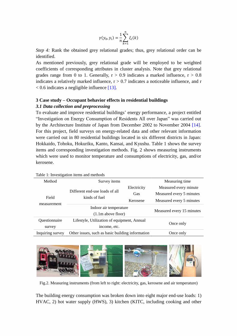
Hokkaido, Tohoku, Hokuriku, Kanto, Kansai, and Kyushu. Table 1 shows the survey

items and corresponding investigation methods. Fig. 2 shows measuring instruments

which were used to monitor temperature and consumptions of electricity, gas, and/or

kerosene.

Table 1: Investigation items and methods

Method Survey items Measuring time

Field

measurement

Different end-use loads of all

kinds of fuel

Electricity Measured every minute

Gas Measured every 5 minutes

Kerosene Measured every 5 minutes

Indoor air temperature

(1.1m above floor) Measured every 15 minutes

Questionnaire

survey

Lifestyle, Utilization of equipment, Annual

income, etc. Once only

Inquiring survey Other issues, such as basic building information Once only

Fig.2. Measuring instruments (from left to right: electricity, gas, kerosene and air temperature)

The building energy consumption was broken down into eight major end-use loads: 1)

HVAC, 2) hot water supply (HWS), 3) kitchen (KITC, including cooking and other

kitchen equipment such as dishwasher and range hood), 4) lighting (LIGHT), 5)

refrigerator (REF), 6) amusement and information (A&I, such as television, telephone,

and computer, etc.), 7) housework and sanitary (HOUSE, such as washing machine,

vacuum, and electrical shaver, etc.), and 8) others (OTHER, unidentified usage such

as electrical shutter and all the unclear items).

Scrutinizing the data from the 80 buildings, researchers found that only 67 sets were

complete, while 13 had missing values of energy consumption data. Data reduction

and aggregation was then performed to obtain a smaller representation of the original

data. For example, diverse energy unit of different kinds of primary energy sources

used by the various buildings, including electricity, natural gas, and kerosene, was

converted to MJ based on conversion coefficients in Table 2 so they could be added

directly. Then, readings of each end-use load at different intervals (e.g., 1 or 5 minutes)

were averaged over each month. The resulting data was stored in a database.

Table 2: Conversion coefficients of different fuels

Fuel Conversion coefficient Unit

Electricity 3.6 MJ/kWh

City gas (4A-7C) 20.4 MJ/Nm3

City gas (12A-13C) 45.9 MJ/Nm3

Liquefied petroleum gas (LPG) 50.2 MJ/Nm3

Kerosene 36.7 MJ/L

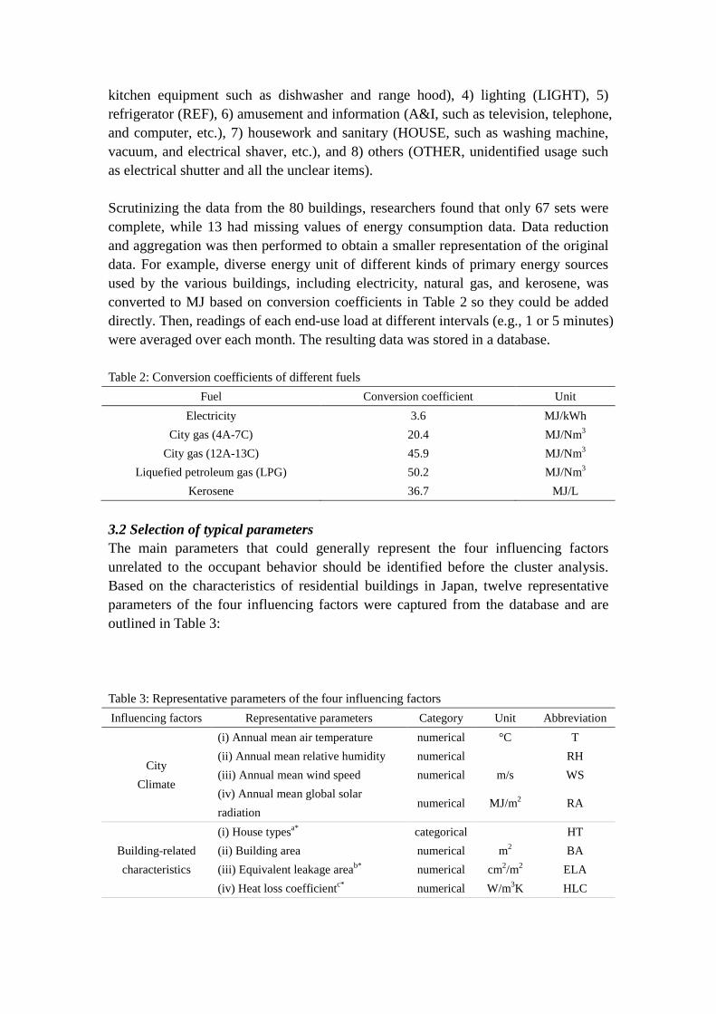
3.2 Selection of typical parameters

The main parameters that could generally represent the four influencing factors

unrelated to the occupant behavior should be identified before the cluster analysis.

Based on the characteristics of residential buildings in Japan, twelve representative

parameters of the four influencing factors were captured from the database and are

outlined in Table 3:

Table 3: Representative parameters of the four influencing factors

Influencing factors Representative parameters Category Unit Abbreviation

City

Climate

(i) Annual mean air temperature numerical °C T

(ii) Annual mean relative humidity numerical RH

(iii) Annual mean wind speed numerical m/s WS

(iv) Annual mean global solar

radiation numerical MJ/m

2 RA

Building-related

characteristics

(i) House typesa*

categorical HT

(ii) Building area numerical m2 BA

(iii) Equivalent leakage areab*

numerical cm2/m

2 ELA

(iv) Heat loss coefficientc*

numerical W/m3K HLC

User-related

characteristics

except social and

economic factors

(i) Number of occupants numerical NO

Building services

systems and

operationd*

Energy source of usage for

(i) Space heating and cooling categorical HC

(ii) Hot water supply categorical HWS

(iii) Kitchen equipment categorical KE

a*) House types are divided into either detached house or apartment.

b*) Measured by the fan pressurization method.

c*) Calculated based on building design plans.

d*) Energy source of usage is divided into either electric or non-electric. Since all of the space cooling

equipment is electric, the value of HC is determined by space heating equipment.

3.2 Results and discussion

3.2.1 Grey relational grades

The ultimate goal of this study is to identify the influences of the occupant behavior

on the building energy consumption. Therefore, annual building energy use intensity

(EUI) in 2003 was selected as the objective sequence in GRA, and accordingly, there

is no need to consider the building area independently. Among the remaining eleven

parameters, four weather parameters are time-series variables that can be viewed as a

function of time. In order to take both the impact of season and regional climate

difference into consideration, grey relational grades were first calculated for each

building based on monthly building EUI and local monthly weather parameters [15];

then, an average was taken over grey relational grades in each district. For the other

seven parameters, considering the size of database, grey relational grades were

calculated on all the buildings.

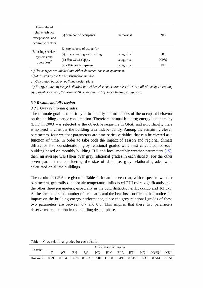
The results of GRA are given in Table 4. It can be seen that, with respect to weather

parameters, generally outdoor air temperature influenced EUI more significantly than

the other three parameters, especially in the cold districts, i.e. Hokkaido and Tohoku.

At the same time, the number of occupants and the heat loss coefficient had noticeable

impact on the building energy performance, since the grey relational grades of these

two parameters are between 0.7 and 0.8. This implies that these two parameters

deserve more attention in the building design phase.

Table 4: Grey relational grades for each district

District Grey relational grades

T WS RH RA NO HLC ELA HTa*

HCb*

HWSb*

KEb*

Hokkaido 0.799 0.584 0.620 0.683 0.701 0.780 0.490 0.617 0.537 0.514 0.551

Tohoku 0.831 0.555 0.765 0.662

Hokuriku 0.772 0.532 0.644 0.716

Kanto 0.737 0.601 0.732 0.641

Kansai 0.712 0.580 0.695 0.690

Kyusyu 0.654 0.605 0.661 0.675

a* The two states of house types, i.e., detached house and apartment, are transformed to [0, 1].

b* The two states of these three parameters, i.e., electrical and non-electrical, are transformed to [0, 1].

3.2.2 Cluster analysis

After data preprocessing and the calculation of the grey relational grades, i.e.

weighted coefficients of the selected parameters in Table 3, cluster analysis was

conducted using the open-source data mining software WEKA. The results of cluster

analysis are given in Table 5. With the consideration of the size of the database, four

clusters were determined by the K-means algorithms based on Euclidean distance

measures. Cluster centroids, which represent the mean value for each dimension, were

used to characterize the clusters. For example, it can be seen that cluster 1, in

comparison with the other clusters, is a segment of buildings representing a high

outdoor air temperature (the cluster centroid of T in this cluster is 0.609, which is

higher than that in the other three clusters), detached houses (the cluster centroid of

HT in this cluster is 0, indicating that all the buildings in this cluster are detached

house), high heat loss coefficients, low equivalent leakage areas, small number of

occupants, non-electrical hot water supplies and kitchen equipment, etc. Similarly, the

other clusters can be explained as follows: cluster 2 can be mainly characterized as

high solar radiation, large number of occupants, electrical space heating and cooling,

and electrical kitchen equipment. Cluster 3 is a segment of buildings representing a

low outdoor air temperature, low heat loss coefficients, high equivalent leakage area,

and non-electrical hot water supplies. Cluster 4 can be mainly characterized as high

outdoor relative humidity, non-electrical space heating and cooling, and electrical

kitchen equipment. In addition, the centroid of all the data is also given for

comparison with the cluster centroids, as shown in Full Data column in Table 5. The

internal cohesion and external separation for the clusters based upon the eleven

attributes imply that these attributes have the most similar holistic effects on the

building energy performance in the same cluster, while the effects are significantly

distinct for the buildings in different clusters.

Table 5

Centroid of each cluster and statistics on the number and percentage of instances assigned to

different clusters

Attribute Full Data Cluster

1 2 3 4

T 0.451 0.609 0.483 0.312 0.408

WS 0.313 0.316 0.303 0.339 0.302

RH 0.395 0.262 0.417 0.428 0.439

RA 0.347 0.318 0.370 0.343 0.343

HT 0.166 0.000 0.134 0.411 0.116

HLC 0.183 0.254 0.154 0.116 0.229

ELA 0.394 0.291 0.413 0.460 0.390

NO 0.275 0.216 0.320 0.234 0.296

HC 0.305 0.331 0.000 0.501 0.537

HWS 0.307 0.514 0.067 0.514 0.289

KE 0.222 0.551 0.000 0.514 0.000

Clustered instances and proportion 67 (100%) 13 (19%) 23 (34%) 15 (22%) 16 (24%)

3.2.3 Effects of occupant behavior

3.2.3.1 End-use load shapes

After the generation of four clusters, different end-use loads of various buildings in

each cluster were averaged over one year. Fig. 3 shows the average annual EUI of

different end-use loads for each cluster. The proportion of each end-use load to the

whole is also given above the corresponding bar.

Fig. 3. Average annual EUI of different end-use loads

As shown in Fig. 3, hot water supply and HVAC form the two largest categories of

end-use loads in terms of average annual EUI in all four clusters, while housework

and sanitary and ‘others’ have a modest contribution. Also, the two largest loads far

exceed the other six end-use loads that do not have significant variations in the

proportion among most of the clusters. This indicates that occupants in different

clusters had similar behavior. Moreover, the proportions of both hot water supply and

HVAC remain approximately steady among these clusters, except that there is a

noticeable increase in the HVAC proportion in Cluster 4, which is mainly

characterized by medium-low outdoor air temperature and non-electrical space

heating equipment. This increase may be partly caused by two factors: 1) the high

electricity rate in Japan, and 2) the high efficiency of non-electrical space heating

devices such as kerosene space heaters. A high electricity rate tends to restrict

occupants’ usage of electrical heating/cooling equipment in the other three clusters,

while high efficiency of non-electrical space heating devices encourages occupants’

utilization of them in Cluster 4, thereby increasing energy consumption. Therefore, a

rational combination of electricity rates and primary heating/cooling sources could

help reduce building energy consumption through influencing occupant behavior.

25

% 37

%

9%

11

%

7%

5%

5%

3%

29

%

37

%

10

%

7%

6%

5%

2%

4%

28

%

34

%

7%

9%

7%

7%

3%

4%

41

%

33

%

6%

6%

5%

5%

2%

1%

0

50

100

150

200

HV

AC

HW

SLI

GH

TK

ITC

REF

A&

IH

OU

SEO

THER

HV

AC

HW

SLI

GH

TK

ITC

REF

A&

IH

OU

SEO

THER

HV

AC

HW

SLI

GH

TK

ITC

REF

A&

IH

OU

SEO

THER

HV

AC

HW

SLI

GH

TK

ITC

REF

A&

IH

OU

SEO

THERA

ver

age

annual

EU

I o

f

dif

eren

t en

d-u

se l

oad

s

(MJ/

m2)

End-use loads

Cluster 4 Cluster 3 Cluster 2 Cluster 1

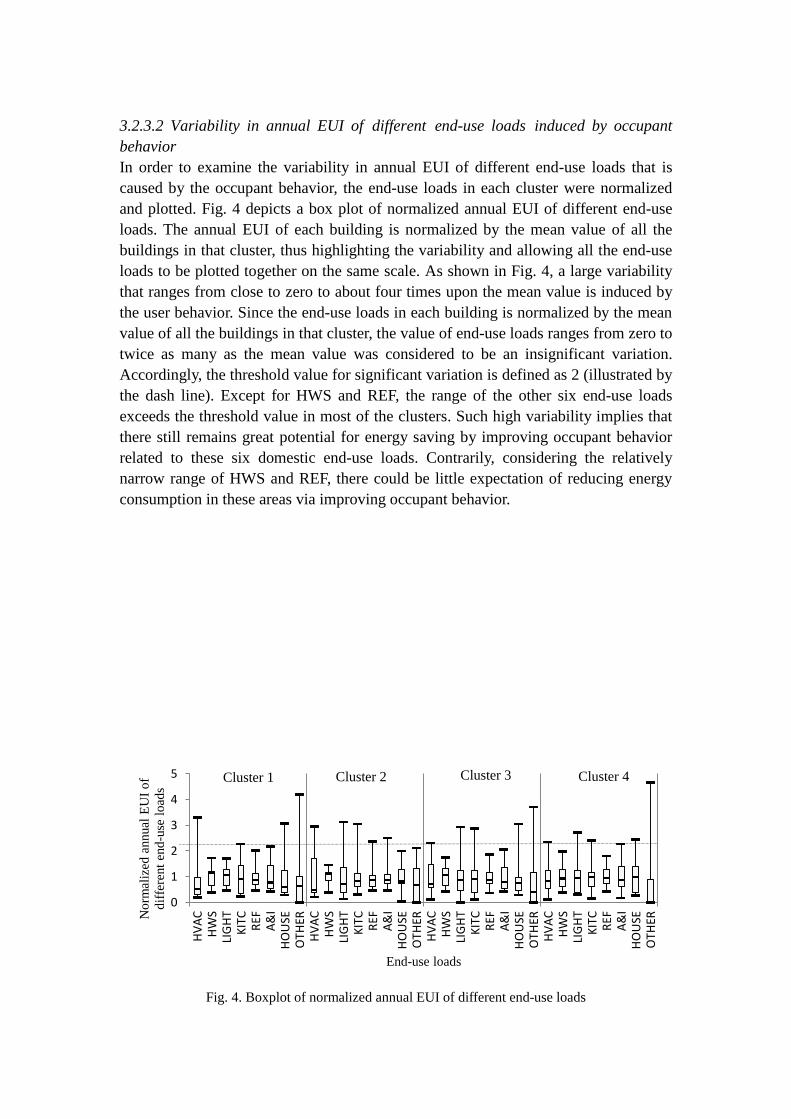
3.2.3.2 Variability in annual EUI of different end-use loads induced by occupant

behavior

In order to examine the variability in annual EUI of different end-use loads that is

caused by the occupant behavior, the end-use loads in each cluster were normalized

and plotted. Fig. 4 depicts a box plot of normalized annual EUI of different end-use

loads. The annual EUI of each building is normalized by the mean value of all the

buildings in that cluster, thus highlighting the variability and allowing all the end-use

loads to be plotted together on the same scale. As shown in Fig. 4, a large variability

that ranges from close to zero to about four times upon the mean value is induced by

the user behavior. Since the end-use loads in each building is normalized by the mean

value of all the buildings in that cluster, the value of end-use loads ranges from zero to

twice as many as the mean value was considered to be an insignificant variation.

Accordingly, the threshold value for significant variation is defined as 2 (illustrated by

the dash line). Except for HWS and REF, the range of the other six end-use loads

exceeds the threshold value in most of the clusters. Such high variability implies that

there still remains great potential for energy saving by improving occupant behavior

related to these six domestic end-use loads. Contrarily, considering the relatively

narrow range of HWS and REF, there could be little expectation of reducing energy

consumption in these areas via improving occupant behavior.

Fig. 4. Boxplot of normalized annual EUI of different end-use loads

0

1

2

3

4

5

HV

AC

HW

SLI

GH

TK

ITC

REF

A&

IH

OU

SEO

THER

HV

AC

HW

SLI

GH

TK

ITC

REF

A&

IH

OU

SEO

THER

HV

AC

HW

SLI

GH

TK

ITC

REF

A&

IH

OU

SEO

THER

HV

AC

HW

SLI

GH

TK

ITC

REF

A&

IH

OU

SEO

THERN

orm

aliz

ed a

nnual

EU

I o

f

dif

fere

nt

end

-use

lo

ads

End-use loads


3.2.3.3 Reference building and energy-saving potential

In order to evaluate energy-saving potential for the four clusters, the reference

building for each cluster was first defined. The characterization of the reference

building was carried out by identifying the building with the energy consumption

closest to the cluster energy consumption centroid in terms of Euclidean distance and

end-use loads. The annual EUI of different end-use loads of a reference building for

each cluster is given in Table 6.

Table 6

Annual EUI of different end-use loads of reference building for each cluster (MJ/m2)

HVAC HWS LIGHT KITC REF A&I HOUSE OTHER SUM

Cluster 1 77 165 31 24 25 12 29 0 363

Cluster 2 45 161 39 25 22 20 7 12 332

Cluster 3 154 141 33 42 20 13 6 0 409

Cluster 4 188 212 34 25 15 19 11 0 504

Fig. 5. Stacked-column diagram of annual EUI of different end-use loads of three typical buildings

Fig. 5 shows the stacked-column diagram of annual EUI of different end-use loads of

three typical buildings in the four clusters: a reference building (RB) and buildings

with the minimum (Min) and maximum (Max) annual EUI. Occupant behavior led to

a huge difference between these three different buildings in each cluster. In this study,

annual EUI of different end-use loads of a reference building was taken as a baseline.

Accordingly, the energy-saving potential of a building with a larger annual EUI than

that of a reference building could be determined by computing the difference between

them. For example, the potential energy savings that could be achieved by improving

occupant behavior for the buildings with the maximum annual EUI in the four clusters,

i.e. EUIMax – EUIRB, were 281 MJ/m2, 250 MJ/m

2, 198 MJ/m

2, and 202 MJ/m

2,

respectively. Moreover, comparison with a reference building provided a means of

examining which end-use load seemed to have the greatest potential for energy

conservation. For instance, comparison between the building with the maximum

0

100

200

300

400

500

600

700

800

Min RB Max Min RB Max Min RB Max Min RB MaxAnnual

EU

I o

f d

iffe

rent

end

-use

load

s (M

J/m

2)

Reference building and buildings with the minimum and maximum EUI

OTHER

HOUSE

A&I

REF

KITC

LIGHT

HWS

HVAC


annual EUI and the reference building in each cluster indicated that HVAC

contributed the most towards energy saving, while HWS had a negligible contribution.

This result is consistent with the conclusion drawn from Fig. 3. Similarly, other

end-uses loads with noticeable energy-saving potential in each cluster could be

identified, such as housework and sanitary in Cluster 1 and lighting in Cluster 4. Such

information can help building owners realize that which occupant behavior should be

modified in practice to effectively improve building energy performance. Further,

based on this information, a better effect may be achieved if building occupants

receive an energy-saving education and tips on how to improve their behavior. It

should be noted that, in comparison with a reference building, buildings with the

minimum annual EUI in the four clusters not only had lower HVAC EUI, but also had

much smaller HWS EUI. A possible explanation for this is that occupants in these

buildings reduced energy consumption by being concerned about the cost in living

standards. For example, these occupants may decrease the frequency of utilization of

room air conditioners in the cooling season, even though the indoor temperature is not

the best comfort temperature. Further field investigation is needed to identify the real

reasons.

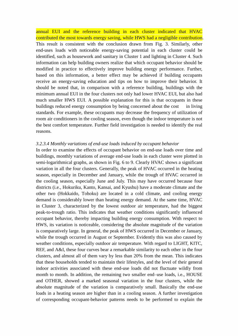
3.2.3.4 Monthly variations of end-use loads induced by occupant behavior

In order to examine the effects of occupant behavior on end-use loads over time and

buildings, monthly variations of average end-use loads in each cluster were plotted in

semi-logarithmical graphs, as shown in Fig. 6 to 9. Clearly HVAC shows a significant

variation in all the four clusters. Generally, the peak of HVAC occurred in the heating

season, especially in December and January, while the trough of HVAC occurred in

the cooling season, especially June and July. This may have occurred because four

districts (i.e., Hokuriku, Kanto, Kansai, and Kyushu) have a moderate climate and the

other two (Hokkaido, Tohoku) are located in a cold climate, and cooling energy

demand is considerably lower than heating energy demand. At the same time, HVAC

in Cluster 3, characterized by the lowest outdoor air temperature, had the biggest

peak-to-trough ratio. This indicates that weather conditions significantly influenced

occupant behavior, thereby impacting building energy consumption. With respect to

HWS, its variation is noticeable, considering the absolute magnitude of the variation

is comparatively large. In general, the peak of HWS occurred in December or January,

while the trough occurred in August or September. Evidently this was also caused by

weather conditions, especially outdoor air temperature. With regard to LIGHT, KITC,

REF, and A&I, these four curves bear a remarkable similarity to each other in the four

clusters, and almost all of them vary by less than 20% from the mean. This indicates

that these households tended to maintain their lifestyles, and the level of their general

indoor activities associated with these end-use loads did not fluctuate wildly from

month to month. In addition, the remaining two smaller end–use loads, i.e., HOUSE

and OTHER, showed a marked seasonal variation in the four clusters, while the

absolute magnitude of the variation is comparatively small. Basically the end-use

loads in a heating season are higher than in a cooling season. A further investigation

of corresponding occupant-behavior patterns needs to be performed to explain the

reasons for this variation.

Fig. 6. Monthly variation of end-use loads in Cluster 1



10

100

1000

10000

Jan. Feb. Mar. Apr. May Jun. Jul. Aug. Sep. Oct. Nov. Dec.

End

-use

lo

ads

(MJ)

Month

HVAC

HWS

LIGHT

KITC

REF

A&I

HOUSE

OTHER

10

100

1000

10000


End

-use

lo

ads

(MJ)

Month

HVAC

HWS

LIGHT

KITC

REF

A&I

HOUSE

OTHER

10

100

1000

10000


End

-use

lo

ads

(MJ)

Month

HVAC

HWS

LIGHT

KITC

REF

A&I

HOUSE


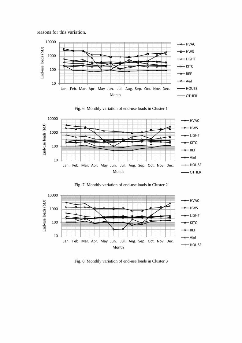
3.2.3.5 Monthly average indoor temperature of air-conditioned room

Different occupant behavior, especially those associated with HVAC, can significantly

affect indoor climate, which in turn will have an influence on occupant behavior,

thereby causing dramatic differences in building energy consumption. Therefore, the

effects of occupant behavior on building energy consumption should be understood

and interpreted in conjunction with the investigation of indoor climate. Figures 10–13

show the monthly average living-room temperature of three typical buildings in each

cluster: the reference building (RB) and buildings with the maximum and minimum

annual EUI (Max and Min). These selected living rooms had air conditioners and/or

heating equipment. As shown in Fig. 10, there is a significant difference between

living-room temperatures of the three buildings in the cooling season and a minor

difference in other seasons. The living room of Max was maintained at a temperature

of about 24 °C in the cooling season. At the same time, the room temperature of Min

was around 5 °C higher than that of Max, and the room temperature of RB was

generally between that of Max and Min in this season. Considering that Cluster 1 is

characterized by the highest outdoor air temperature, it can be deduced that the

frequency of utilization of room air conditioners in the cooling season in these three

buildings can be ranked as: Max > RB > Min. With respect to the other three clusters,

Fig. 11–13 shows that the living room of Max was maintained at a temperature of

about 24 °C all year, while living-room temperatures of RH and Min varied with the

outdoor air temperature. Clearly the frequency of utilization of space cooling/heating

equipment in the three buildings in these three clusters has the same order as that in

Cluster 1 in both heating and cooling seasons. These results suggest that occupant

behavior that seeks thermal comfort normally results in high energy consumption.

Therefore, there has to be a trade-off between human thermal comfort and building

energy consumption, and it is necessary to strike a balance between achieving a high

comfort level and reducing energy consumption through modifying occupant

behavior.

10

100

1000

10000


End

-use

lo

ads

(MJ)

Month

HVAC

HWS

LIGHT

KITC

REF

A&I

HOUSE

OTHER

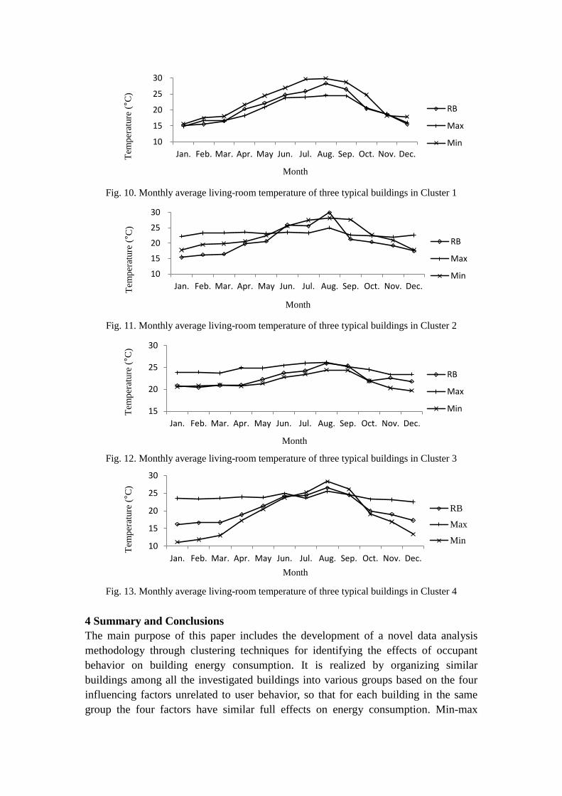
Fig. 10. Monthly average living-room temperature of three typical buildings in Cluster 1




4 Summary and Conclusions

The main purpose of this paper includes the development of a novel data analysis

methodology through clustering techniques for identifying the effects of occupant

behavior on building energy consumption. It is realized by organizing similar

buildings among all the investigated buildings into various groups based on the four

influencing factors unrelated to user behavior, so that for each building in the same

group the four factors have similar full effects on energy consumption. Min-max

10

15

20

25

30

Jan. Feb. Mar. Apr. May Jun. Jul. Aug. Sep. Oct. Nov. Dec.Tem

per

ature

(°C

)

Month

RB

Max

Min

10

15

20

25

30


Tem

per

ature

(°C

)

Month

RB

Max

Min

15

20

25

30


Tem

per

ature

(°C

)

Month

RB

Max

Min

10

15

20

25

30


Tem

per

ature

(°C

)

Month

RB

Max

Min

normalization techniques are performed as a data preprocessing step to deal with the

inconsistencies of different attributes. Grey relational analysis is also carried out, and

grey relational grades, a measure of relevancy between two factors, are used as

weighted coefficients of attributes in cluster analysis.

In order to demonstrate its applicability, this methodology was applied to a group of

residential buildings located in six different districts of Japan. Energy-related data of

these buildings was measured, and a database was developed after scrutinizing the

measured data. Twelve attributes were captured from the database to represent the

influencing factors unrelated to occupant behavior. K-means method was selected in

cluster analysis and four clusters were obtained as a result.

In these four clusters the effects of occupant behavior on building energy consumption

were examined at the end-use level. End-use variations over time and buildings

induced by occupant behavior were analyzed. Also, as a preliminary step toward

identifying energy-saving potential, a reference building was defined as the building

whose energy consumption was the closest to cluster energy consumption centroid in

terms of Euclidean distance and end-use loads. Moreover, indoor climate was

investigated to better understand and interpret the effects of occupant behavior.

This proposed method allows researchers to evaluate building energy-saving potential

by improving user behavior, and provides multifaceted insights into building energy

end-use patterns associated with occupant behavior. The results obtained could help

prioritize efforts of modification of occupant behavior to reduce building energy

consumption, and also could be used to improve modeling of user behavior in

numerical simulation.

The main focus of future research should be placed on identifying appropriate

building sample sizes and number of clusters, selecting typical attributes that can

adequately represent the influencing factors unrelated to occupant behavior, since

these measures will provide more precise effects of occupant behavior. In addition,

more case studies in different sectors, such as commercial buildings and office

buildings, should be conducted to further improve building energy performance and

policy formulation.

Acknowledgements

The authors would like to express their gratitude to the Public Works and Government

Services Canada, and Concordia University for the financial support.

References

[1] C. F. Reinhart, Lightswitch-2002: a model for manual and automated control of electric

lighting and blinds, Solar Energy 77 (1) (2004), pp. 15–28.

[2] D. Bourgeois. Detailed occupancy prediction, occupancy-sensing control and advanced

behavioral modeling within whole-building energy simulation. Ph.D. thesis, l’Universite Laval,

Quebec, 2005.

[3] H. B. Rijal, P. Tuohy, M. A. Humphreys, J. F. Nicol, A. Samuel, J. Clarke, Using results from

field surveys to predict the effect of open windows on thermal comfort and energy use in buildings,

Energy and Buildings 39 (7) (2007), pp. 823–836.

[4] P. Hoes, J. L. M. Hensen, M. G. L. C. Loomans, B. de Vries, D. Bourgeois, User behavior in

whole building simulation, Energy and Buildings 41(3) (2009), pp. 295–302.

[5] H. Nakagami, Lifestyle change and energy use in Japan: Household equipment and energy

consumption, Energy 21(12) (1996), pp. 1157–1167.

[6] L. Lopes, S. Hokoi, H. Miura, K. Shuhei, Energy efficiency and energy savings in Japanese

residential buildings – research methodology and surveyed results, Energy and Buildings 37(7)

(2005), pp. 698–706.

[7] Z. Yu, F. Haghighat, B. C. M. Fung, H. Yoshino, A decision tree method for building energy

demand modeling, Energy and Buildings 42(10) (2010), pp. 1637–1646.

[8] A. F. Emery, C. J. Kippenhan, A long-term study of residential home heating consumption and

the effect of occupant behavior on homes in the Pacific Northwest constructed according to

improved thermal standards, Energy 31(5) (2006), pp. 677–693.

[9] J. Ouyang, K. Hokao, Energy-saving potential by improving occupants' behavior in urban

residential sector in Hangzhou City, China, Energy and Buildings 41(7) (2009), pp. 711–720.

[10] J. Han, M. Kamber, Data mining concepts and techniques, Elsevier Inc., San Francisco

(2006).

[11] WEKA, The University of Waikato. Software, http://www.cs.waikato.ac.nz/ml/weka/

[12] J. Deng, Introduction to grey system, Journal of Grey System 1 (1989), pp. 1–24.

[13] C. Fu, J. Zheng, J. Zhao, W. Xu, Application of grey relational analysis for corrosion failure

of oil tubes, Corrosion Science 43(5) (2001), pp. 881–889.

[14] http://www.data.jma.go.jp/obd/stats/data/en/smp/index.html

[15] Climate Statistics, Japan Meteorological Agency. Monthly Mean and Monthly Total Tables,

http://www.data.jma.go.jp/obd/stats/data/en/smp/index.html

http://www.data.jma.go.jp/obd/stats/data/en/index.html

http://www.data.jma.go.jp/obd/stats/data/en/smp/index.html

a systematic procedure to study the influence of occupant behavior on building energy

Documents