A Tale of Two Tails:Commuting and the Fuel Price Response in Driving∗

Kenneth Gillingham, Yale University, NBER, and CESIfoAnders Munk-Nielsen, University of Copenhagen

September 28, 2018

Abstract

Pricing greenhouse gases is widely understood as the most efficient approach formitigating climate change, yet distributional effects hamper political acceptance. Thesedistributional effects are especially important in transport, the fastest growing sector forgreenhouse gas emissions. Using rich data covering the entire population of vehicles andhouseholds in Denmark, this study uncovers an important feature of driving demand:two groups of much more responsive households in the lower and upper tails of thework distance distribution. We further estimate the causal effect of public transport–acritical determinant of the upper tail–and show how public transport access can bothreconcile differences in fuel price elasticities between the United States and Europe,and considerably influence the distributional effects of fuel pricing.

Keywords: distributional effects, transportation, commuting, urban form, environ-mental taxes.JEL classification codes: R4, R2, Q4, H2, L9

∗Gillingham: Yale University, NBER, and CESIfo, 195 Prospect Street, New Haven, CT 06033 USA,kenneth.gillingham@yale.edu; Munk-Nielsen: University of Copenhagen, Department of Economics, ØsterFarimagsgade 5, 26.3.01, DK-1353 Copenhagen K, Denmark, anders.munk-nielsen@econ.ku.dk. The authorswish to thank Bertel Schjerning, John Rust, Matthew Kotchen, Ismir Mulalic, Fedor Iskhakov, and SørenLeth-Petersen, as well as numerous seminar participants, for helpful comments and feedback. The authorswould also like to acknowledge funding from the IRUC research project, financed by the Danish Council forStrategic Research.

1

“Relocation is part of the solution to a serious problem. That growth and jobs are toounevenly distributed between country and city. It creates a risk of Denmark being rippedapart.” - Lars Løkke Rasmussen, Prime Minister of Denmark, 19 October 2016 (on thegovernment’s plan to relocate public sector jobs)

1 Introduction

Greenhouse gas emissions from transportation amount to a quarter or more of all anthro-pogenic emissions in many countries around the world, and this share is rapidly growing.From 1990 to 2015, the share of greenhouse gas emissions from transport has increased from15 percent to 26 percent in Europe and from 23 percent to 27 percent in the United States(EEA, 2017; EPA, 2017). With continued declines in the cost of renewables and continueddecarbonization of the electricity sector, this trend is likely to continue and perhaps evenaccelerate. Thus, policymakers worldwide have become increasingly attentive to the trans-port sector. Economists are uniformly in support of pricing greenhouse gases as the first-bestapproach to mitigate greenhouse gas emissions. Yet, political acceptance of pricing policiesis often hampered by concerns about the distributional effects of such policies, and this isespecially true for pricing transportation fuel consumption (Borenstein, 2017). A commonconcern is that pricing policies will disproportionately affect a subset of households, such asless-wealthy households outside of urban areas.

This study uses millions of vehicle-level odometer readings matched to individual-leveldemographic information from the Danish registers to ask several questions. How do house-holds across the population change their driving in response to fuel price changes? How isthis response influenced by access to public transport? And what does the heterogeneity inresponse mean for the distributional effects of fuel price changes? We uncover a new findingto the literature: two groups of households who are much more responsive to changing fuelprices than most of the population. These households are in the tails of the work distancedistribution; one group has the longest commutes and the other commutes very little. Ourmean medium-run (one-year) elasticity estimate of -0.30 is considerably influenced by thesetwo groups of tail households, each of which are much more elastic. These findings can berationalized by switching costs incurred when substituting from driving to other modes oftransport, such as public transport, and we estimate the causal effect of public transport ondriving responsiveness. Danes have almost universal access to public transport and we positthat our results hold in similar settings around the world.

Our results have direct policy implications. By uncovering the economic mechanisms atwork in the driving elasticity, we show that the two groups of tail households face substantially

2

reduced impacts from fuel price increases. This is especially important because the roughly15% of the population in the upper tail–households with the longest commutes–face a heavyburden from fuel price increases and thus may be more opposed to pricing greenhouse gases.This is a politically salient point in Denmark as the Danish government pays particularly closeattention to rural voters who tend to have longer commutes. As was noted by Prime MinisterRasmussen, the Danish government is even going as far as moving 3,900 governmental jobsto outside the capital region at a cost of over 400 million DKK ($61 million at the July 9,2017 exchange rate).1 These issues are by no means isolated to Denmark, with the impact ongroups of voters outside of cities playing a key role in policy debates about pricing greenhousegases throughout the developed world.

Indeed, our findings also have implications for other countries where access to publictransport is less universal. Our results suggest that access to public transport is a prerequisitefor the existence of the upper tail. Without adequate access to public transport, householdswith long commutes are less able to substitute away from driving when fuel prices rise.Intuitively, previous work from countries with more limited access to public transport, suchas the United States, show no evidence of the upper tail of responsiveness from householdswith longer commutes. Such previous work does however routinely find that households incities (who would be expected to have shorter commutes) tend to be more responsive (e.g.,Kayser, 2000; Gillingham, 2013, 2014; Gillingham, Jenn, and Azevedo, 2015), consistent withour lower tail, which we show is also primarily driven by households in the cities in Denmark.By identifying the upper tail in the work distance distribution in Denmark, we show thatthere is a group of more-responsive households in Europe that is not likely to exist in countrieslike the United States where public transport provision is lower. This directly impacts theeffectiveness of fuel pricing in reducing driving and emissions and may crucially affect thepolitical acceptability of pricing greenhouse gases.

This research contributes to several strands of literature. First, there is a growing lit-erature on the distributional effects of policies to reduce greenhouse gas emissions from thetransportation sector. Economists have worked on this issue for decades, primarily focusingon the vertical distributional effects (i.e., distributional effects over income) of gasoline taxes(Poterba, 1989, 1991). More recently, Borenstein and Davis (2016) estimate the distribu-tional effects of U.S. Clean Energy Tax Credits (including subsidies for hybrid and electricvehicles) and find them to be quite regressive. Levinson (2016), Jacobsen (2013), and Davisand Knittel (2016) compare the vertical distributional impacts of fuel economy standards togasoline taxes in the United States, generally finding that fuel economy standards are more

1See the Danish factsheet: https://www.regeringen.dk/aktuelle-dagsordener/udflytning-af-statslige-arbejdspladser/se-status-paa-udflytning/.

3

regressive than gasoline taxes.2 There is much less work on geographic distributional conse-quences, despite the importance for policy. Bento et al. (2009) use survey data to estimatethe efficiency and distributional consequences of gasoline taxes across states in the UnitedStates and show that households in more rural states face a much higher burden. Our studyis the first to identify the two tails of more responsive drivers, link them to geographic loca-tion, shed light on the mechanisms creating them, and show how they influence the short-rundistributional effects of policies affecting fuel prices.

This study also uses rich data to provide a new point estimate for the fuel price elasticityof driving, which is a dominant component in the modeling of gasoline or diesel demand.Understanding the responsiveness to fuel prices is a first-order question in economics. Notonly is it valuable for anticipating responses to future swings in oil prices, it is also usefulfor measuring the macroeconomic effects of oil price fluctuations (e.g., Edelstein and Kilian,2009) and providing insight into the role of speculators during oil price shocks (Hamilton,2009). Not surprisingly, there is a vast literature aiming to estimate the price elasticityof gasoline demand (e.g., for some recent studies see Coglianese et al., 2016; Davis andKilian, 2011; Hughes, Knittel, and Sperling, 2008; Li, Linn, and Muehlegger, 2014; Hymeland Small, 2015; Small and van Dender, 2007; Levin, Lewis, and Wolak, 2017). Most ofthese studies use aggregate data at the regional or national level.3 More recently, severalstudies have estimated the elasticity of vehicle-miles-traveled with respect to the price ofgasoline using disaggregated micro-level data, either from surveys or inspection odometerreading data (e.g., Linn, 2016; Bento et al., 2009; Gillingham, 2013, 2014; Munk-Nielsen,2015; De Borger, Mulalic, and Rouwendal, 2016b; Knittel and Sandler, 2018). In a notablecontrast, estimates for drivers in the United States tend to be in the range of -0.05 to -0.30,while similar benchmark estimates for European drivers tend to show a much more elasticresponse. For example, Frondel and Vance (2013) estimate a medium-run driving elasticitywith respect to the gasoline price of -0.45 in Germany.4 Similarly, in contemporaneous work,De Borger, Mulalic, and Rouwendal (2016a) focus on a subsample of two-vehicle householdsin Denmark and find the medium-run fuel price elasticity of driving to range between -0.32and -0.45. We demonstrate how the removal of the upper tail–or the removal of adequateaccess to public transport–can reconcile these differing estimates between the United Statesand Europe.

2There is a substantial literature on the distributional effects of gasoline taxes and carbon taxes, includingHausman and Newey (1995), West (2004), West and Williams (2004), Bento et al. (2009), Sterner (2012),Williams et al. (2015).

3Review articles cover dozens of studies going back decades, most using aggregate data. For example, seeDahl and Sterner (1991), Espey (1998), Graham and Glaister (2004), and Brons et al. (2008).

4-0.45 is the fixed effects estimate, which we believe is better identified than other estimates in the paper,which are closer to -0.6.

4

Our results also contribute to a third vein of literature on the complex relationshipsbetween household location, public transport availability, gasoline prices, and consumer deci-sions about how much to drive. Since at least McFadden (1974), it has long been recognizedthat access to public transport is an important mediator of travel choices, with clear environ-mental implications (e.g., Glaeser and Kahn, 2010). Our work contributes to this literatureby using an instrumental variables strategy to identify the causal effect of public transporton the responsiveness of driving to fuel price changes. Further, there is growing evidence thaturban form and the spatial structure of commuting demand can affect travel mode choices(Bento et al., 2005; Grazi, van den Bergh, and van Ommeren, 2008; Brownstone and Golob,2010). Our paper follows the literature estimating short-run and medium-run driving elastic-ities by holding the household location fixed, but shows how long-run equilibrium commutedistances influence the short-run response to fuel prices.5 These results are important for landuse and transport policy, as they clarify the implications of policies that encourage shortercommute times (e.g., some smart growth policies) or greater access to public transport.

The remainder of this paper is organized as follows. The next section describes the richDanish register data and provides descriptive evidence on the primary features of the datarelevant to estimating the driving responsiveness. Section 3 describes our empirical strategy,while section 4 presents the results and a set of robustness checks. Section 5 discussesimplications for policy, including an illustrative distributional effects analysis. Section 6concludes.

2 Data

2.1 Data Sources

This study is based on rich data from the Danish registers on the population of both house-holds and vehicles in Denmark from 1998 to 2011. There are three main sources. The firstis the vehicle license plate register, which contains the vehicle identification number, grossvehicle weight rating (i.e., maximum operating weight including passengers and cargo), fueltype, date of registration, owner identification number, and whether the vehicle type is apersonal car or a van.6

The second data source is the vehicle inspection database. Since July 1, 1998, all vehicles5We also run a series of robustness checks where we exploit data on household residence and work locations

and changes in these over time, finding that both our mean elasticity and tail results are quite robust.6Company cars are not in our database and are not linked to a person but rather to the firm. However,

individuals with access to a company car must pay a tax for this, and we observe that 3.7% of our householdshave at least one member paying this tax.

5

in Denmark are required to undertake a mandatory safety inspection at periodic intervalsafter the first registration of the vehicle. In Denmark, the first inspection is roughly fouryears out, and subsequent inspections are every other year.7 Only a small number of usedvehicles are imported into Denmark, in part because they pay a large vehicle registration feeand value-added tax that are assessed based on similar new vehicle prices. The fee and taxschedule are based on the value of the vehicle for all vehicles new to Denmark.8 The inspectiondatabase contains odometer readings, which can be used to determine the kilometers drivenbetween two inspections.

The third primary data source is the household register, which contains detailed demo-graphic data at the calendar year-level. These data include the number of members of thehousehold, ages and sex of these members, municipality of the household, income of thehousehold members (including transfers), and a measure of work distance used to calculatethe tax deduction for work travel.9 On Danish tax forms, households must report theirhome address, workplace address, and number of days that work travel occurred (regardlessof mode of transport). Multiplying the door-to-door work distance by the number of daysyields a measure of work distance that accounts for how much total commuting is actuallyoccurring. We then divide by 225 to give a measure of the effective average work distance ina workday. This measure is particularly useful because a household that lives very far awayfrom work but rarely ever physically commutes (e.g., teleworks most of the time) would havea low (average) work distance by this measure. The tax authorities take this measure seri-ously, with random audits of employers, and checks on the home and work addresses, so it isconsidered a highly reliable measure. One downside of this measure is that the individual isonly eligible for a deduction if the distance is greater than 12 kilometers but there is no min-imum requirement on the number of days that travel to work occurred. The work distancemeasure will therefore be equal to zero if the individual lives closer than 12 kilometers fromthe work place or if the individual does not travel to their workplace. If an individual livesfurther than 12 kilometers and only occasionally commutes, it is possible for the measure tobe between 0 and 12.

For 2000 to 2008, we also have data on the actual work distance for 79.6% of the households7This is a very similar schedule to inspections in states in the United States, such as California. Details

about the driving period lengths are in Appendix A.1.2. We control for the length of the period and performrobustness checks subsampling on the period length.

8After 2007, the vehicle registration fee assessed at the time of the transaction is also adjusted based onthe fuel economy of the vehicle.

9For couples, there is a separate work distance variable for the male and female of the couple. In thesecases, we use the maximum work distance of the two members but have also performed robustness checks toconfirm that this does not appreciably change the primary results.

6

measured using a door-to-door shortest-path algorithm and provided by Statistics Denmark.10

This second measure provides a useful check on our first measure, especially for householdswith commutes under 12 kilometers (See Appendix A.3.3). However, the actual work distancemeasure is a flawed measure for understanding the commute length of long work distancehouseholds, for some of these households may work from home or in nearby locations, andthus rarely travel the full commute. Fortunately, our robustness checks suggest similar resultsregardless of which measure we use.

In addition to the register data, we also bring in daily price data for 95 octane gasolineand diesel fuel from the Danish Oil Industry Association.11 Similarly, we also bring in dailyWest Texas Intermediate crude oil price data for a robustness check.12 Finally, we use datafrom Journey Planner on all bus and train stops in Denmark in 2013.13 This is a singlecross-section, but there were no substantial Denmark-wide changes in public transport overour time period; there were only minor extensions of certain lines and other tweaks to thesystem, as will be discussed further below.

We also have access to some additional car characteristics, including fuel economy inkilometers/liter and the manufacturer suggested retail price (MSRP). These data are fromthe Danish Automobile Dealer Association (DAF). However, these variables are not availablefor car vintages older than 1997. Finally, we bring in historical municipality-level populationdata from 1916 from Statistics Denmark.

2.2 Development of the Final Dataset

We combine the data from the various sources to create a final dataset where the unitof observation is a vehicle driving period between two inspections. So if a driver has afirst inspection of her vehicle on June 1, 2004 and the next inspection on June 6, 2006,the driving period will be the 735 days between these two tests. We use the difference inodometer readings between these two inspections to calculate the total kilometers driven andthe kilometers driven per day over the driving period. Similarly, we calculate the averagegasoline, diesel, and oil price over the same driving period. If a car changes owners during adriving period, we include an observation for both households that have contributed to thedriving and a variable for the fraction of the driving period the car is held by each owner.

To match our calendar year demographic data with driving periods, we construct aweighted average of the values of the demographic variables over the years covered by the

10Statistics Denmark has access to the actual addresses of individuals. This information, however, isanonymized in our dataset so we cannot perform any operations based on GIS information.

11See www.eof.dk, Accessed June 17, 2015.12See www.eia.gov/dnav/pet/hist/LeafHandler.ashx?n=PET&s=RWTC&f=D, Accessed June 15, 2015.13See www.journeyplanner.dk, Accessed April 19, 2013.

7

driving period. For example, if a driving period covers half of 2001, all of 2002, and half of2003, the values of the demographic variables would be given a weight of 0.25 for 2001, 0.5for 2002, and 0.25 for 2003. The density of public transport stops is added to the data atthe municipality level.

The final dataset after cleaning consists of 5,855,446 driving period observations coveringnearly all driving periods by Danish drivers over the period from 1998 to 2011. Table 1presents summary statistics for the final dataset. For our estimations, we demean all of thevariables in order to facilitate interactions. Appendix A provides further details on the datasources and cleaning process.

2.3 Descriptive Evidence

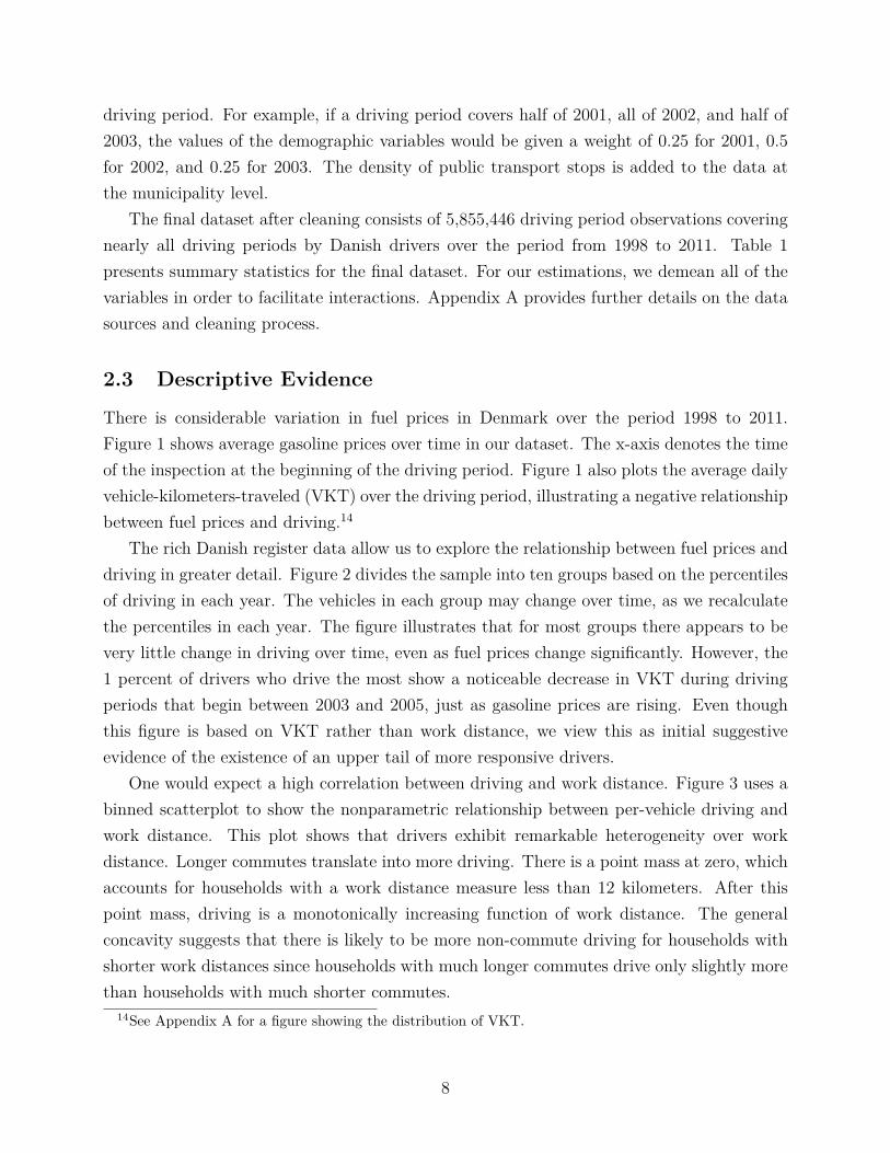
There is considerable variation in fuel prices in Denmark over the period 1998 to 2011.Figure 1 shows average gasoline prices over time in our dataset. The x-axis denotes the timeof the inspection at the beginning of the driving period. Figure 1 also plots the average dailyvehicle-kilometers-traveled (VKT) over the driving period, illustrating a negative relationshipbetween fuel prices and driving.14

The rich Danish register data allow us to explore the relationship between fuel prices anddriving in greater detail. Figure 2 divides the sample into ten groups based on the percentilesof driving in each year. The vehicles in each group may change over time, as we recalculatethe percentiles in each year. The figure illustrates that for most groups there appears to bevery little change in driving over time, even as fuel prices change significantly. However, the1 percent of drivers who drive the most show a noticeable decrease in VKT during drivingperiods that begin between 2003 and 2005, just as gasoline prices are rising. Even thoughthis figure is based on VKT rather than work distance, we view this as initial suggestiveevidence of the existence of an upper tail of more responsive drivers.

One would expect a high correlation between driving and work distance. Figure 3 uses abinned scatterplot to show the nonparametric relationship between per-vehicle driving andwork distance. This plot shows that drivers exhibit remarkable heterogeneity over workdistance. Longer commutes translate into more driving. There is a point mass at zero, whichaccounts for households with a work distance measure less than 12 kilometers. After thispoint mass, driving is a monotonically increasing function of work distance. The generalconcavity suggests that there is likely to be more non-commute driving for households withshorter work distances since households with much longer commutes drive only slightly morethan households with much shorter commutes.

14See Appendix A for a figure showing the distribution of VKT.

8

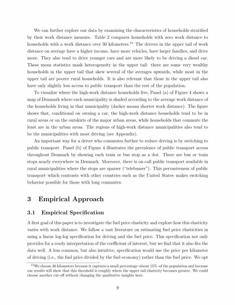
We can further explore our data by examining the characteristics of households stratifiedby their work distance measure. Table 2 compares households with zero work distance tohouseholds with a work distance over 30 kilometers.15 The drivers in the upper tail of workdistance on average have a higher income, have more vehicles, have larger families, and drivemore. They also tend to drive younger cars and are more likely to be driving a diesel car.These mean statistics mask heterogeneity in the upper tail: there are some very wealthyhouseholds in the upper tail that skew several of the averages upwards, while most in theupper tail are poorer rural households. It is also relevant that those in the upper tail alsohave only slightly less access to public transport than the rest of the population.

To visualize where the high-work distance households live, Panel (a) of Figure 4 shows amap of Denmark where each municipality is shaded according to the average work distance ofthe households living in that municipality (darker means shorter work distance). The figureshows that, conditional on owning a car, the high-work distance households tend to be inrural areas or on the outskirts of the major urban areas, while households that commute theleast are in the urban areas. The regions of high-work distance municipalities also tend tobe the municipalities with most driving (see Appendix).

An important way for a driver who commutes further to reduce driving is by switching topublic transport. Panel (b) of Figure 4 illustrates the prevalence of public transport accessthroughout Denmark by showing each train or bus stop as a dot. There are bus or trainstops nearly everywhere in Denmark. Moreover, there is on-call public transport available inrural municipalities where the stops are sparser (“telebusser”). This pervasiveness of publictransport–which contrasts with other countries such as the United States–makes switchingbehavior possible for those with long commutes.

3 Empirical Approach

3.1 Empirical Specification

A first goal of this paper is to investigate the fuel price elasticity and explore how this elasticityvaries with work distance. We follow a vast literature on estimating fuel price elasticities inusing a linear log-log specification for driving and the fuel price. This specification not onlyprovides for a ready interpretation of the coefficient of interest, but we find that it also fits thedata well. A less common, but also intuitive, specification would use the price per kilometerof driving (i.e., the fuel price divided by the fuel economy) rather than the fuel price. We opt

15We choose 30 kilometers because it captures a small percentage–about 15%–of the population and becauseour results will show that this threshold is roughly where the upper tail elasticity becomes greater. We couldchoose another cut-off without changing the qualitative insights here.

9

not to use this specification because we do not observe fuel economy for a sizable portion ofthe sample.16

Consider the demand for driving for vehicle i in household h during a driving period t,which may cover several years y. Recall that a driving period is simply the period in betweentwo odometer readings. We model the demand for driving as follows:

log VKTiht = γ log pft + xihtβ + φ(f, t) + µh + εiht. (1)

VKTiht is the average daily driving in kilometers, xiht denotes a vector of controls, and pft isthe average daily fuel price over the driving period t for the fuel type f ∈ {gasoline, diesel}of vehicle i. The coefficient γ is our primary coefficient of interest–the fuel price elasticity.The controls in xiht include variables for work distance, age of members of the household,gross income of members of the household, whether the household lives within one of the fivemajor urban areas of Denmark, number of children, whether the vehicle is a company car,whether the household has at least one self-employed individual, and the density of bus ortrain stops in the municipality. The vector xiht also includes variables for whether and byhow much the driving period overlaps with other driving periods by the same household.17

We use φ(f, t) to denote fuel type-specific time controls. We consider several differenttypes of time controls with increasing flexibility and our results are robust to which type weuse. In the simplest case, we use a linear time trend in the mid-date of the driving period.A more flexible control uses year dummies for the mid-date of the driving period to allowa non-linear trend in average driving. We can then include a second set of year dummiesinteracted with a dummy for diesel fuel to allow the effect to be fuel-type specific. Next,we include year dummies equal to one if the driving period overlaps with the calendar yearfor even a single day. However, if a driving period only has a single day in a year, it wouldnaturally be affected less by whatever unobserved time-factors affecting driving in that year.Thus, we examine a specification that includes year variables that are equal to the fractionof the driving period that takes place in the given year. These fuel-type specific year controls

16We also include household-vehicle fixed effects in a robustness check, and these fixed effects removeany vehicle-specific time-invariant factors, such as fuel economy. Our resulting elasticity is nearly identical.Further, we examine specifications where all covariates are included in logs as well as specifications where allcovariates enter in levels, and again find similar results.

17Recall that if the car changes owner mid-way through the driving period, the driving period is included asan observation by both households and we add a control for the percent of the driving period each householdowns the car. We also add controls for ownership of other vehicles that do not admit driving observationssuch as motorcycles, mopeds, trailers, etc.

10

are what we use in our preferred specification.18

In addition to the year controls, we also include controls for the length of the drivingperiod as well as a dummy for whether the driving period is the first observation for thecar (i.e., it is a new car), the car age, and the fraction of the driving period that it wasowned by the current household. The controls for the length of the driving period may beparticularly helpful for directly addressing any mean reversion due to shorter driving periodshaving greater variance in VKT. Finally, µh are household fixed effects.19

3.2 Identification

Of primary interest in this paper is discerning whether there is important heterogeneity inthe relationship between driving and fuel price that influences the short-run distributionalimpacts of price changes. Our gasoline and diesel fuel price variables are time series variables,as there is negligible cross-sectional variation in fuel prices across Denmark. The primarysource of the time series variation in these refined fuel price variables is variation in oilprices, as oil is the feedstock for gasoline and diesel production. Any remaining variation inthe refined fuel prices may be due to Denmark-specific shocks to refining or fuel demand. Theoil price is determined on the global market and Denmark is a small market, so it reasonablyfollows that Denmark-specific shocks are not likely to affect the global oil price. However,localized shocks may influence the non-oil price-related variation in the refined fuel prices. Inaddition, there may be correlated demand shocks across countries. For example, a commondemand shock in Northern Europe due to a macroeconomic shock would be represented inthe refined fuel price time-series variation.

These localized shocks and correlated demand shocks are likely to be a small part of thefuel price variation. Nevertheless, we consider each carefully. We address common regionaldemand shocks that may influence both driving and oil prices with our flexible time controls,and we perform a series of robustness checks with different time controls. We address thepossibility of endogeneity due to localized shocks by performing a robustness check in which

18To illustrate these, if a driving period starts in the middle of 2001 and ends in the middle of 2003, thenthe controls will be 0.25 for 2001 and 2003 and 0.5 for 2002 and zero for all other years. These variables areinterpreted exactly like year dummies but are more flexible in the sense that they accommodate the fact thatour driving periods can have different lengths and may cover a given year to a smaller or greater extent. Forclarity, note that if all driving periods started on Jan 1 and ended on Dec 31 the same year, there would beno difference between our time controls and using year dummies. Our effects are not fully flexible, however:the effect of covering 2003 by 10% is the same whether those 10% are in the start of the year or the endof the year. We have also estimated a specification with dummies at the year-and-month level, but if wefurthermore allow each of these dummies to vary by fuel type, there is almost no variation left in the pricevariable.

19Note that only 15% of households in Denmark own more than one vehicle, so household fixed effects arenearly the same as household-vehicle fixed effects.

11

we instrument for the refined fuel price with the global oil price. Specifically, we use theWTI oil price index, which is based in the United States and captures variation in global oilprices that is quite removed from localized shocks in Denmark.

As fuel prices are an aggregate Denmark-wide variable, one might be concerned aboutother macroeconomic dynamics, such as fuel prices affecting the macroeconomy and thusindirectly affecting driving. Fortunately, we have access to panel data on household-levelincomes, which are a far more precise variable to use to account for how macroeconomic shocksaffect consumer decisions than commonly used variables such as GDP or unemployment.Importantly, our income variable is time-varying.20

Our specification includes household fixed effects to nonparametrically address time-invariant unobserved household heterogeneity. These household fixed effects are particularlyimportant for identification because they allow us to focus on within-household variation(deviations from the mean) in driving over time. Any sorting into different locations basedon time-invariant unobserved preferences will be captured by the fixed effects, as will anytime-invariant unobserved household heterogeneity relating to the car choice decision. Thismeans that the variation we use in the work distance variable is purged of longer-term issuesof consumer preferences about where to live and where to work.

In using these household fixed effects, we are identifying our work distance-related coef-ficients largely from households that moved or had their workplace move. The identifyingassumption for these coefficients to be quantifying a causal effect is that households move fora variety of reasons (e.g., for a better job, to be closer to family, to reduce their commute,to buy a house, etc.), but they do not move because of a change in unobserved preferencesfor driving, and similarly, workplaces change for exogenous reasons to the household (e.g.,the company moves or the worker gets a new job). For this identification strategy to beproblematic one must believe that households have a time-varying unobserved preference fordriving that happens to be correlated with the choice to move or change jobs. While thisseems unlikely, it may be possible. Thus, we run a series of robustness checks exploringdifferent sources of variation using subsamples. For example, a firm relocation should be anexogenous shifter of work distance from the household perspective and we find that our basicresults still hold on a subsample of households where only firms relocate.21 We also findsimilar results when we explore a subsample of only households that choose to relocate. Thefact that we get similar results when we utilize these very different sources of variation in the

20We also explore a robustness check where we include municipality-level unemployment, but find thatadding this covariate makes no difference to the fuel price coefficient or the tail.

21We do not use this as our primary specification because of the unusual sample selection (people whohave their firm relocate are not the same as the broader population) and because we lose power from usingthe much smaller sample. The details are in Appendix C.8.

12

work distance over time provides further evidence supporting the validity of our identifyingassumption.

Another possible identification concern is that our variable for public transport access,the density of bus and train stops, is simultaneously determined with driving. For this tobe an issue, the Danish government would have to set public transport access based at leastin part on the expected responsiveness to fuel price in an area. If the Danish governmentset public transport access based on the level of driving, this would be fully addressed bythe household fixed effects. However, it may be possible that the Danish government setpublic transport access based in part on responsiveness, perhaps due to a desire to alleviatecongestion during times of lower fuel prices. To address any possible endogeneity concernrelating to our variable for public transport access, we also examine a specification wherewe instrument for public transport access with municipality-level population data from 1916,which is the earliest year complete municipality-level population data are available.22 Thisapproach follows Duranton and Turner (2011), Mulalic, Pilegaard, and Rouwendal (2015),and other recent papers using historical data that determine the location of rail and roadlines, but otherwise should not influence outcomes today.

A further possible concern is that urban amenities might change over time, and thesechanges could be correlated with both work distance and driving. While most urban amenitiestake decades to develop and can be safely considered constant in our empirical setting, itis possible that some amenities occasionally change. Public transport is an example. Weresearched this possibility carefully. In general, we find that there were few changes tourban amenities over our time period, and public transport also did not change much. AnyDenmark-wide changes would be addressed directly with our time controls, so any concernwould have to be a region-specific change that is correlated with work distance. The onlymeaningful change we uncovered was the addition of a line to the Copenhagen metro between2002 and 2007 (Mulalic, Pilegaard, and Rouwendal, 2015). This would not be captured inour variable for public transport access. If households or firms happened to move in the2007-2011 period because of this expansion of the metro line, this could bias our coefficienton the work distance. Thus, we perform a robustness check in which we remove the GreaterCopenhagen area from our estimation sample, and again find similar results.

A next possible identification concern could be that we are not including controls forvehicle characteristics, such as fuel economy. Given our household fixed effects addressingtime-invariant household preferences for vehicles and the fact that we are using time seriesvariation in fuel prices, this is unlikely to be an issue. This is especially true because in

22See http://www.dst.dk/Site/Dst/Udgivelser/GetPubFile.aspx?id=19910&sid=byersfolk1801,Accessed June 12, 2017.

13

Denmark only a small percentage of households have more than one car (less than 15%),so household fixed effects are extremely similar to vehicle fixed effects. However, we alsoexamine a robustness check with household-vehicle fixed effects to address any unobservedheterogeneity at the vehicle (rather than household) level, which again provides similar resultsonly on a smaller subsample and with somewhat less power. Regarding multi-car households,we observe and control for the number of cars, motorcycles, mopeds, campers, vans, andtrailers.

4 Results

4.1 The Mean Elasticity of Driving

Table 3 shows the results from estimating the linear fixed effects model in equation (1). A richset of controls are included in the estimation, but for brevity, we report selected coefficients.Column (1) is the most parsimonious specification, which only controls for seasonality (%of the driving period covering each month), the driving period, and car characteristics. Thecoefficient on the log fuel price indicates a fuel price elasticity of driving of -0.87. Whenwe add year controls and demographics in column (2), the elasticity changes to -0.30. Thisindicates the importance of controlling for individual-level demographics as well as usingtime controls. In columns (3) and (4), we add household fixed effects with and without timecontrols. Without the time controls, the elasticity is -0.51. Adding time controls bringsthe elasticity to -0.30, which is our preferred estimate and can be interpreted as a medium-run or one-year elasticity. It may not be surprising that the elasticity moves closer to zerowhen we nonparametrically control for general time trends in driving since larger economictrends could be correlated with both driving and fuel prices.23 The ability to simultaneouslycontrol for household fixed effects and time controls is a unique advantage of our data, whichcombines full population data with a over a decade time horizon.

It is worth noting that we find the same fuel price elasticity in columns (2) and (4), whichare identical except for the addition of household fixed effects. We take this as an indicationthat our rich set of controls are capturing the most important determinants of the fuel priceelasticity. In particular, we expect that the variables for work distance, company cars, andpersonal income capture key components of driving demand.

As was also seen in our descriptive analysis, Table 3 shows that driving is increasing inwork distance. Even the dummy for whether the work distance is non-zero (recall that it

23In Appendix Table 15 we show that the elasticity is robust to the exact functional form of the timecontrols. In fact, even in a specification with just a linear time trend in the starting year of the period, theelasticity is -0.31.

14

is censored at 12 km based on how the data are collected) has a positive and statisticallysignificant coefficient. The results indicate that increasing the work distance by one additionalkm can be interpreted as increasing daily driving by approximately 0.6%. An increase of onestandard deviation in work distance would correspond to a change in driving of over a thirdof the inter-quartile range–an economically significant effect.24

The statistically significant coefficients on income suggest that increasing income lowersdriving demand for couples, while it increases driving demand for singles. This may be dueto wealthier couples being able to afford to live in more geographically advantageous areas,while singles cannot. However, this effect is economically relatively small, which is importantbecause it indicates that factors such as work distance are more economically significant thaneven income. This provides evidence supporting a focus on commuting in this paper.

The coefficient on the density of bus/train stops per km2 is statistically significant andnegative in columns (2) and (3), which might be expected: better access to public trans-port should reduce driving. However, because access to public transport is so universal inDenmark (recall Figure 4) and public transport access changes so rarely, there is relativelylimited variation in this variable and no time-series variation. When households fixed effectsare included, the remaining identifying variation stems from households that move betweenmunicipalities. Thus, it may not be surprising that in column (4), which includes the year-fuelcontrols, the effect becomes statistically indistinguishable from zero. As discussed above, apossible concern with this specification is that the public transport variable is endogenous. Aswe will see shortly, the estimated fuel price elasticity does not change in our IV specification,further supporting our identification approach here.

A natural question that arises when using the price elasticity for policy analysis is howwell the functional form of the demand curve follows a constant elasticity assumption. Toexplore non-linearities further, Figure 5 plots the non-parametric relationship between logVKT and log fuel price, where both variables have been residualized in a first stage to accountfor partial correlations with remaining regressors.25 A key finding is that over a broad rangeof fuel prices, the functional form in the log-log scale is approximately linear. This supportsboth the use of the log-log specification, as well as the use of the elasticity over a relativelybroad range of fuel price changes. Only at the extremes of fuel price in our data, which areidentified from fewer observations, do we observe a nonlinear relationship. Note that the

24The standard deviation of work distance is 19.7 and the inter-quartile range where it is observed is 19.3.The VKT distribution has standard deviation 40.2, a 25th percentile of 27.7 km, and a 75the percentile of58.2.

25Note that this is different from a partially linear semi-parametric model. The literature includes anumber of estimators for doing this (e.g., Robinson, 1988; Blundell, Horowitz, and Parey, 2012) but standardapproaches do not permit fixed effects, which are key in our setting. This is why we focus on the non-parametric relationship between orthogonalized regressors instead.

15

extremes in fuel price are not the extremes in work distance or VKT, so these extremes areentirely unrelated to our tails. Having a slightly different relationship at very high and verylow fuel prices accords with intuition and underscores that the estimates in this paper shouldbe used with caution when the fuel price is much lower or higher than has been typicallyobserved in our dataset.

4.2 Exploring the Tails

We next explore a similar specification to our primary model in equation (1) that includesinteractions between the log of the fuel price and a subset of controls to better understandthe determinants of the mean elasticity. We denote this subset with x1

iht. The linear modelwith interactions is given by

log VKTiht = γ0 log pft + γ1x1iht × log pft + xihtβ + φ(f, t) + µh + εiht.

In x1iht, we include variables of interest for our interactions, including work distance and

public transport variables. A virtue of this approach is the simplicity of estimation usinga standard fixed effects estimator. One feature of this approach is that the model placesno restrictions on the values of γ0 or γ1, so it is possible to find positive values of the priceelasticity of driving for certain groups of households.26

Table 4 shows the results from estimating the above equation. Column (1) repeats ourprimary results with no interactions. Column (2) adds work distance interactions. Column(3) further adds the public transport density interaction (estimated on the slightly smallersample for which the data including the IV are complete). Column (4) is the same as ourprimary specification in column (1), only it instruments for public transport density withmunicipality population in 1916. The first-stage F-statistic is 49.5, demonstrating that wedo not have a weak instrument concern. Column (5) instruments for public transport density,as well as the interaction of public transport density with the fuel price. Comparing acrosscolumns demonstrates the robustness of our results. Most notably, the elasticity at the mean,presented near the bottom of the table, does not substantially change across columns.

We first focus on the work distance interaction variables. In column (2) in Table 4, weinclude interactions with a quadratic in work distance. All three work distance coefficientsare statistically significant. The interactions of the quadratic in work distance with price

26Blundell, Horowitz, and Parey (2012) formulate a nonparametric estimator that imposes negative elas-ticities, arguing that their findings of an upward sloping demand curve without this restriction must be dueto a small sample size. Our sample size is very large and set of controls extensive, so we prefer to not toimpose any non-negativity constraints on the elasticity. Of course, it is also theoretically possible that somepeople respond to rising fuel prices by increasing their driving (e.g., if driving is a complement to an activitythat is strongly positively correlated with fuel prices).

16

tend to show an essentially decreasing linear slope, while the interaction of the dummy fora non-zero work distance implies an overall relationship that perhaps can be described asan inverted-U. To more clearly illustrate this relationship in a nonparametric fashion, weinteracted the log fuel price with 19 dummies for work distance bins. Figure 6 illustratesthe inverted-U shape. For the shortest work distances (< 12 km), the fuel price elasticity isrelatively high in absolute value at nearly -0.40.27 For slightly longer work distances (longenough where walking and biking are less viable options), the elasticity decreases in absolutevalue around -0.05 (a value comparable to some estimates in the United States). But then itincreases in absolute value again, reaching roughly -0.6 for work distances over 70 km (notethe data begins to become sparser by this point).

Figure 6 visually demonstrates two tails based on work distance. A first tail consists ofhousesholds who own a vehicle but commute very little (either live very close to work or tendto work from home). A second tail consists of households with very long commutes. There isa clear economic intuition that can rationalize these two tails. For the first tail, nearly all ofthe driving is for non-work trips. Unlike trips between home and work, these trips are morelikely to be diverse, which means that drivers may have more opportunities to substitute someof these trips from driving to biking, walking, or public transport (and these trips are likelyto be city driving, which for non-electric hybrid cars is less efficient). For the second tail,smaller increases in fuel prices lead to much larger expenditures on driving, providing a strongincentive to consider substitutes. Both tails influence the mean driving elasticity, althoughthe second tail would be expected to be more important for overall fuel consumption due tothe greater expenditures on fuel by drivers in this upper tail. In Appendix D we develop asimple analytical model of travel decisions to build further intuition for the two tails.

Moving to public transport, Columns (3) and (5) in Table 4 both show that the coefficienton the public transport interaction with fuel price is statistically significant and negative,indicating that increased public transport access increases the responsiveness to fuel pricechanges. In column (5), we are instrumenting for public transport density in both the maineffect and interaction with a valid and strong instrument, and thus we interpret this result asthe causal effect of public transport density on the fuel price responsiveness. The coefficientindicates that an increase of one more bus or train stop per square kilometer will changethe fuel price elasticity by -0.01 (recall the mean number of stops per square kilometer isjust under 16, with a standard deviation of just over 18). Thus, subtracting one standarddeviation from the mean can change the price elasticity by -0.18, which is an economicallylarge difference in responsiveness when the mean elasticity is -0.30. This result is not only to

27This result is robust to using the shortest path measure of work distance, which reassures us that thecoding at zero is not the reason for our finding of the lower tail. Furthermore, the shape is robust to using alog specification in work distance. The details are in Appendix C.10.

17

the best of our knowledge new to the literature, but it also underscores that public transportaccess is a key factor influencing the fuel price responsiveness–a result we will discuss furtherin section 5.

4.3 Geographic Heterogeneity in the Elasticity of Driving

The results thus far indicate two tails, the first of which involves households with longcommutes (upper tail) and the second households who commute very little (lower tail). Onemight expect to see further evidence of the upper tail in a particularly high responsivenessto fuel price changes in the outskirts of cities, where households have the longest commutes.Similarly, a high responsiveness to fuel price changes in urban areas would build furtherevidence supporting our hypothesized mechanism for the lower tail. Figure 7 presents theresults of a geographical analysis, illustrating the spatial location of the most responsivehouseholds. The shading in the figure indicates the predicted elasticity for each observationaveraged over the municipalities (darker is more responsive). The three largest cities arelabeled.

Two key findings emerge from Figure 7. First, some of the most responsive municipalitiesare in the largest cities. This aligns with the above evidence suggesting that there is atail of more responsive drivers with shortest commutes. Second, many of the other mostresponsive municipalities are in the outskirts of cities. For example, the region just north ofCopenhagen has some of the most elastic drivers. These areas tend to have wealthy, high-educated households who often drive for their commute to jobs in Copenhagen. Access topublic transport is excellent (recall Figure 4). Similar findings emerge for other areas in theoutskirts of urban areas, further building evidence in support of the existence of an uppertail.

4.4 Robustness Checks

We perform an extensive set of robustness checks to confirm our primary results. They aresummarized briefly here and discussed in more detail in the Appendix. They broadly confirmour preferred point estimate of the fuel price elasticity, -0.30. Moreover, in our tests, we findthat the result of the two tails generally continues to hold. Table 5 provides an overview ofthe different robustness checks, showing the highest and lowest elasticities that came out ineach case; in many cases, the extreme elasticities are to be expected, so we discuss them inthe text below, going through each case in turn.

Our first robustness check examines the time window of our sample. Rather than usingdriving periods that start between July 1998 and December 2007 (which run through 2011),

18

we estimate the same model either starting the sample as late as 2001 or ending the sampleas early as 2004. The results bound our preferred estimate in a relatively narrow window:-0.40 to -0.28. The differences may be due to a time-varying elasticity as much as to a lackof robustness. Our second check examines a subsample of the data either controlling for orrestricting the sample to driving periods that are of a typical length, which in our settingis two years or four years, plus or minus three months. Our estimated elasticity is quiterobust and demonstrates that timing of the inspections is not an identification concern. SeeAppendix C.1 for full results. The result of the two tails holds for these robustness checks.

The empirical design in this study models both gasoline and diesel car users. This essen-tially imposes the restriction that drivers of the two different types of cars respond similarlyto the fuel price regardless of whether it is gasoline or diesel. The resulting mean elasticityis more useful from a policy perspective, but it masks differences in how diesel and gaso-line vehicles are driven. We thus perform a third robustness check where we estimate thesame model in equation (1) separately for diesels and gasoline vehicles. We also examine aspecification with an interaction between the log fuel price and a diesel dummy. The inter-action shows that the gasoline price elasticity is -0.26, while for the diesel segment it is -0.38.Estimating on separate samples yields corresponding elasticities of -0.27 and -0.55. Thesefindings demonstrate that the elasticity is not primarily identified by the differential betweengasoline and diesel fuel prices. They also highlight that the diesel segment is more pricesensitive, which is consistent with the story behind the two tails since diesel drivers tend tohave longer commutes. We perform a similar robustness check for a couples subsample and asingles subsample, finding elasticities of -0.32 and -0.20 respectively. In both cases, the uppertail persists, although the upper tail loses statistical significance in the subsample of singlesand diesel cars, perhaps not surprisingly given how much of the data (including many of thepeople in the tails) are excluded.

The year controls employed in equation (1) are highly flexible, which is important forcontrolling for potentially correlated time-varying factors, but is also demanding on the data.We thus run robustness checks where we examine alternative time controls (see AppendixC.4). We find that the results are robust to removing our seasonality controls (the % of eachmonth controls) and even removing the year controls for diesel vehicles. When we reduce thetime controls to a single linear trend we find estimated elasticity of -0.31. The elasticity isalso unchanged if we use year dummies based on the midpoint of the driving period. Bothtails remain in all of these checks.

Next, we consider the possibility that fuel prices are endogenous. Denmark is a smallcountry buying both gasoline and diesel on the larger European market, so it is not likelythat Denmark-specific demand shocks lead to an endogeneity issue. However, it is possible

19

that such an issue may occur. Thus, our robustness check instruments the fuel price usingthe WTI crude oil price, which is not only physically located in the United States, but isdetermined by global oil market movements (see Appendix C.6). It is hard to imagine asmall localized demand shock in Denmark possibly affecting the WTI crude oil price. At thesame time, the first stage regression indicates that it is a strong instrument, since oil is theprimary feedstock for refined fuel. The 2SLS fuel price elasticity estimate is a statisticallysignificant -0.36. This estimate is close to our preferred estimate of -0.30, and we view this asconfirming our estimate. Given the standard errors, these two estimates are not statisticallysignificantly different.

One possible concern with our study is that we use the work distance variable reported ontax returns and households with work distances less than 12 kilometers are not eligible for thededuction, so are coded to zero. While we are very confident that this coding is done correctly(due to the threat of random audits) our primary results do not have much variation betweenzero and 12 kilometers. Thus, we also estimate our model using the 79.6% subsample forwhich we have the actual distance between the home and workplace using a shortest-distancealgorithm. The estimated elasticity is -0.37 and again is not statistically significantly differentfrom our preferred estimate of -0.30, confirming our estimate on the larger sample using thebetter measure that captures intensity of commuting. Equally importantly, the result of thetwo tails again holds using this alternative work distance measure (see Appendix C.10).

We also perform a series of robustness checks examining the possibility of selection intodifferent vehicles that may lead car characteristics to be endogenous (e.g., see Gillingham(2013) or Munk-Nielsen (2015)). We find our results quite robust to the exact choice ofvehicle characteristics that are included. More importantly, we also run a specification withhousehold-vehicle fixed effects, which would address any concern about the inclusion or ex-clusion of any particular vehicle characteristic, such as fuel economy. The estimated elasticityis -0.31 and the tail story continues to hold, confirming that our results are robust, albeitwith some loss of statistical significance due to the smaller sample (see Appendix C.7).

Next, we consider the source of variation over time in the work distance measure. Weexplore different sources of variation, estimating the model on subsamples of only householdsthat choose to relocate or only households where the firm of at least one spouse relocates atsome point during the sample.28 These are much smaller subsamples that are useful for un-derstanding the variation driving our results. Using the 49,074 observation subsample whereonly the firm relocates, we find a mean elasticity of -0.36. Using the 3,244,793 observationsubsample where a household moves, we find a mean elasticity of -0.41. In both cases, the

28A relocation is defined by Statistics Denmark based on a change in address for the firm or one of thefirm’s work locations, or if the work location of all workers in one location changed to a different locationwithin the same firm.

20

two tails based on work distance are still present and the original mean elasticity is withinthe 95% confidence interval (due to the substantially higher standard error on the estimates).The details are in Appendix C.8.

Finally, we examine the possibility that gasoline prices affect driving both directly, througha consumer response to the price at the pump, and indirectly, through macroeconomic effects.Our empirical specification includes personal income at the household level as a covariate,which should address macroeconomic effects that may influence driving. We first addedmunicipality-level unemployment as another covariate to the specification run in column 4of Table 3. The coefficient on the log fuel price changes from -0.301 to -0.299 and is againstatistically significant. The work distance interaction coefficients are again identical to arounding error, indicating that the tail remains. We also include register data measure ofunemployment as controls (see Appendix C.9), and the estimate only changes from -0.301 to-0.298 with the tail estimates similarly unchanged.

Second, we explored the relationship between unemployment rates and fuel prices byregressing the unemployment rate on fuel prices. When we look at the correlation without anyother covariates, we see a very small and negative relationship. When we add further controls,especially time controls, the coefficient on fuel price becomes statistically insignificant. Whilenot definitive, we view these findings as suggestive that fuel prices seem to have relativelylittle effect on the unemployment rate in the Danish economy. We further divide the sampleinto four bins based on the average work distance of the municipality and run the sameregression of the unemployment rate on the fuel price on each subsample. We again finda small effect, and importantly, the effect is roughly the same over the four bins of workdistance. This suggests that the effect of fuel prices on the unemployment rate does not varybased on commuting distance.

Third, we ran a type of placebo test by collecting data on the price of other fuels that mightalso influence the economy but that are not used for driving. We ran the same regression asin column 4 of Table 3 only we also include covariates for the log of the natural gas price andthe log of three coal prices for coal that is occasionally imported into Northern Europe: fromthe United States, Australia, and South Africa.29 For all four prices (regardless of whetherwe include them separately or together), we find that the coefficient values are very closeto zero and statistically insignificant. This provides further evidence that the results we arefinding are from fuel prices influencing directly influencing driving, rather than influencingthe broader economy and indirectly influencing driving.

29The source of the natural gas prices is Statistics Denmark, while the source of the coal prices is the U.S.Energy Information Administration.

21

5 Implications for Policy

In this section, we discuss the implications for policy of our results. The finding of the twotails is particularly important in light of discussions in Europe about carbon taxation. Aneconomy-wide carbon tax would raise the price of fossil fuels in all sectors, including transport.Perhaps the most challenging political obstacle to carbon pricing is the potential for perversedistributional consequences. Vertical distributional consequences (i.e., across income) areclearly important, but what we emphasize here is that distributional consequences acrossgeography due to differences in work distance can also be very important. As has been well-documented in the news, in many countries around the world–including Denmark–there ispolitical discontent in areas outside of the large cities. For example, most of the votes forBrexit in the United Kingdom were from areas outside of London and other large cities. Thereis similar discontent in Denmark, with the anti-immigration party receiving the most votesin areas outside of the largest cities. Politicians in Denmark have been acutely aware of thisdiscontent and have gone to great lengths to provide support for these areas. For example,they have moved thousands of government jobs away from the capital region urban center, ata cost of millions of dollars. Thus, the differing distributional effects over geography–whichare influenced greatly by the work distance–are directly relevant for the political acceptabilityof any policy that disproportionately impacts poorer rural regions more, including carbonpricing.

The tails have clear implications for the differing distributional effects. The upper tailis especially important for it tends to consist of drivers who live outside of the major urbanareas and who drive relatively more (just under 15% of the population). These upper tailhouseholds face a high burden from fuel prices and a disproportionately higher burden whenfuel prices rise. Thus, we perform a simple set of illustrative calculations to demonstrate theimportance of our finding of the upper tail. The focus here is on short-run equilibria; the muchlonger-run relationships between location choice, labor markets, and driving responsivenessare outside the scope of this analysis.

For illustrative purposes, we focus our analysis on the short-run effects of an increase infuel taxes that leads the fuel price to rise by 1 DKK/l for both gasoline and diesel.30 Theaverage gasoline price over the 1998 to 2008 period is 9.01 in 2005 DKK, so this representsa substantial price increase, but it is within the range of the variation in our data.31 Witha fuel price elasticity of driving of -0.30, the proposed increase of 1 DKK/l translates into

30This construction sidesteps issues of passthrough; this equal a 1 DKK/l tax if the passthrough rate was100%.

31This maps to an increase in gasoline prices of $0.57 per gallon based on the June 18, 2015 exchange rateof 6.54 DKK per dollar.

22

a 3.3% short-run reduction in driving (it could be expected to be larger in the long-run).If this occurred due to a tax policy, then fuel tax revenue would increase by 13.2%.32 Weabstract from externalities in this analysis in order to focus on distributional effects.

5.1 Distributional Effects

We focus on the distributional impacts on consumers, calculating both the transfers fromconsumers to the government (i.e., government revenue, calculated as (p1 − p0)V KT (p1))and the direct loss in consumer surplus from reducing the amount driven (

∫ p1p0V KT (p) −

V KT (p1)dp).33 Ignoring externalities, these two quantities combined amount to the changein consumer surplus (∆CS) prior to any redistribution of revenues. In Denmark, the revenuesfrom fuel taxes are added to the general fund, for use on all government spending. Forillustrative purposes, we assume that the funds are redistributed (or provided in equivalently-valued services) on an equal basis to households, an assumption that is reasonable for theDanish setting. Figure 8 provides a simple graphical presentation of the two areas beingcalculated (note in our calculations, we are not imposing linearity on the demand curve).

Table 6 shows the effects of the increase in fuel prices due to the fuel tax broken down bywork distance group. A key finding emerges from this analysis: Households in the upper tailof the work distance distribution are more able to substitute away from driving to reducetheir tax burden, as shown by the greater direct change in consumer surplus (∆CS in column(1)). They drive much more (compare the the upper tail to the full sample in column (2)),but can substitute away from driving to a greater degree, consistent with a larger discreteshift to public transport. This comes about from a flatter demand curve, implying a largerdirect loss in consumer surplus, but a greater ability to avoid the tax by changing behavior.

Of course, the revenue from the transfer is not lost, but can be used for a variety ofpurposes or redistributed. For illustrative purposes, we calculated the effects of a uniformredistribution. We find that those in the upper tail face a much larger burden from the fueltax policy than average (-15 DKK per household per day), while those in the lowest tailreceive a gain (5.82 DKK per household per day). Quantifying these effects is crucial forunderstanding the political acceptability of carbon taxes and more broadly the distributionaleffects after redistribution is a question that policymakers in Denmark care deeply about.Compensatory policies, such as a policy that redistributes more of the revenue to the upper

32At 9 DKK/l, the increase of 1 DKK/l is 11.1%, which at an elasticity of -0.30 translates to a change indriving of 3.33%. Over the sample period, taxes make up 64.87% of the gasoline price, corresponding to 5.84DKK/l at 9 DKK/l. An increase in 1 DKK/l thus corresponds to an increase of 17.13% in taxes, giving atotal relative change in taxes of (1 + 0.1713)× (1− 0.0333) = 13.2%.

33This direct loss in consumer surplus is the Harberger triangle or deadweight loss assuming that Danesare price-takers for fuel and that any externalities have already been internalized from previous taxes.

23

tail, would be necessary if the policy goal is an an equal distributional effects by group.In contrast to the above results, we can see in Figure 9 that this illustrative policy is

actually quite progressive from a vertical equity standpoint, with a higher burden faced bywealthier households. This underscores the usefulness of focusing on more than just verticaldistributional equity.

A natural question is how the Danes have come to accept taxes in excess of 50% of theprice at the pump. We posit that public transport may play a key role. Our causal estimateof the effect of public transport on price sensitivity indicates that while the average elasticityis -0.30, if we reduce the public transport density by one standard deviation, the averageelasticity becomes -0.13. Thus, public transport is instrumental in providing householdswith options for avoiding the large fuel taxes. A second implication though is that fuel taxesare especially distorting for households in the upper tail in leading to changes in behavior(which may be efficiency-improving to the extent that there are uninternalized externalities).

5.2 Public Transport and Reconciling Elasticities

Our results are also insightful for reconciling elasticities between Europe and the UnitedStates (recall the literature reviewed in section 1). First, note that in Figure 6 the averageelasticity outside of the two tails is closer to zero than -0.3 and for much of the sample, closerto zero than -0.2. This squarely puts the elasticity in the range of elasticities commonlyestimated in the United States. Our estimate of the causal impact of public transport providesan insight into why.

Recall that we also performed a simulation that reduces the density of public transport inDenmark by one standard deviation. This change brings the density to roughly in the rangeof levels common in the United States, and thus sheds light on the extent to which publictransport can reconcile the elasticities. We found that the elasticity becomes -0.13. Thisfinding helps to further bridge a gap in the literature by helping to reconcile the differencesbetween elasticity estimates that are an important input to policy.

6 Conclusion

This paper uncovers two tails of more responsive drivers than most of the population inDenmark. The first tail is a small group of consumers living in the outskirts of cities withlong commutes, but adequate access to public transport. The second tail is a group of driverswho commute very little and tend to live in cities. There is an economic intuition for eachof these tails: households with long commutes can readily switch to public transport, while

24

households who commute very little largely use their vehicles for a diverse set of non-worktrips, many of which can easily be switched to other modes of transport. Households that arenot in these two tails tend to be much more inelastic in their response to fuel price changes.

This finding is important for two reasons. First, it is particularly relevant for the politicaleconomy of carbon pricing. Those in the upper tail face the largest burden from a rise infuel prices, but access to public transport allows them to more readily substitute away fromdriving, thereby reducing their burden. Our illustrative calculations quantify the importanceof this effect, showing how ample access to public transport reduces the burden on the uppertail through access to an appealing substitute.

Second, the finding of the two tails helps to reconcile the results of studies in Europe andthe United States that estimate fuel price elasticities. Most studies in the United States showfuel price elasticities in the range of -0.10 to -0.30, while those in Europe over the same timeframe generally tend to be higher in absolute value. Our preferred mean price elasticity valueis -0.30, but we estimate the causal impact of public transport to show that if we removeample access to public transport, this elasticity changes to -0.13, which is much more in linewith recent estimates from the United States for short-run fuel price elasticities of driving.One implication of these results is that if the United States improved its public transportopportunities, the upper tail of responsiveness could emerge there as well, potentially reducingsome of the political challenges to fuel taxation and carbon pricing.

25

References

Bento, Antonio, Maureen Cropper, Ahmed Mushfiq Mobarak, and Katja Vinha. 2005. “TheEffects of Urban Spatial Structure on Travel Demand in the United States.” Review ofEconomics and Statistics 87(3):466–478.

Bento, Antonio, Lawrence Goulder, Mark Jacobsen, and Roger von Haefen. 2009. “Distri-butional and Efficiency Impacts of Increased US Gasoline Taxes.” American EconomicReview 99(3):667–699.

Blundell, Richard, Joel Horowitz, and Matthias Parey. 2012. “Measuring the Price Respon-siveness of Gasoline Demand: Economic Shape Restrictions and Nonparametric DemandEstimation.” Quantitative Economics 3 (1):29–51.

Borenstein, Severin. 2017. “Creative Pie Slicing To Address Climate Policy Opposition.”Energy Institute at Haas Blog .

Borenstein, Severin and Lucas Davis. 2016. “The Distributional Effects of US Clean EnergyTax Credits.” In Tax Policy and the Economy, Volume 30. University of Chicago Press,191–234.

Brons, Martijn, Peter Nijkamp, Eric Pels, and Piet Rietveld. 2008. “A Meta-analysis of thePrice Elasticity of Gasoline Demand. A SUR Approach.” Energy Economics 30 (5):2105–2122.

Brownstone, David and Thomas Golob. 2010. “The Impact of Residential Density on VehicleUsage and Energy Consumption.” Journal of Urban Economics 65 (1):91–98.

Coglianese, John, Lucas Davis, Lutz Kilian, and James Stock. 2016. “Anticipation, TaxAvoidance, and the Price Elasticity of Gasoline Demand.” Journal of Applied Econometricsforthcoming.

Dahl, Carol and Thomas Sterner. 1991. “Analysing Gasoline Demand Elasticities: A Survey.”Energy Economics 13 (3):203–210.

Davis, Lucas and Lutz Kilian. 2011. “Estimating the Effect of a Gasoline Tax on CarbonEmissions.” Journal of Applied Econometrics 26 (7):1187–1214.

Davis, Lucas and Chris Knittel. 2016. “Are Fuel Economy Standards Regressive?” NBERWorking Paper 22925 .

26

De Borger, B., I. Mulalic, and J. Rouwendal. 2016a. “Substitution between cars within thehousehold.” Transportation Research A 85:135–156.

De Borger, Bruno, Ismir Mulalic, and Jan Rouwendal. 2016b. “Measuring the Rebound Effectwith Micro Data: A First Difference Approach.” Journal of Environmental Economics andManagement 79:1–17.

Duranton, Gilles and Matthew Turner. 2011. “The Fundamental Law of Road Congestion:Evidence from the US.” American Economic Review 101 (6):2616–52.

Edelstein, Paul and Lutz Kilian. 2009. “How Sensitive Are Consumer Expenditures to RetailEnergy Prices.” Journal of Monetary Economics 56 (6):766–779.

EEA. 2017. “Greenhouse Gas Emissions from Transport Indicator Assessment.” EuropeanEnvironment Agency .

EPA. 2017. “Inventory of U.S. Greenhouse Gas Emissions and Sinks: 1990-2015.” U.S.Environmental Protection Agency .

Espey, Molly. 1998. “Gasoline Demand Revisited: An International Meta-analysis of Elas-ticities.” Energy Economics 20 (3):273–295.

Frondel, Manuel and Colin Vance. 2013. “Re-Identifying the Rebound: What about Asym-metry?” Energy Journal 34 (4):43–54.

Gillingham, Kenneth. 2013. “Selection on Anticipated Driving and the Consumer Responseto Changing Gasoline Prices.” Yale University Working Paper .

———. 2014. “Identifying the Elasticity of Driving: Evidence from a Gasoline Price Shock.”Regional Science & Urban Economics 47 (4):13–24.

Gillingham, Kenneth, Alan Jenn, and Ines Azevedo. 2015. “Heterogeneity in the Responseto Gasoline Prices: Evidence from Pennsylvania and Implications for the Rebound Effect.”Energy Economics 52 (S1):S41–S52.

Glaeser, Edward and Matthew Kahn. 2010. “The Greenness of Cities: Carbon DioxideEmissions and Urban Development.” Journal of Urban Economics 67 (3):404–418.

Graham, Daniel and Stephen Glaister. 2004. “Road Traffic Demand Elasticity Estimates: AReview.” Transport Reviews 24 (3):261–274.

Grazi, Fabio, Jeroen van den Bergh, and Jos van Ommeren. 2008. “An Empirical Analysisof Urban Form, Transport, and Global Warming.” The Energy Journal 29 (4):97–122.

27

Hamilton, James. 2009. “Understanding Crude Oil Prices.” Energy Journal 30 (2):179–206.

Hausman, Jerry and Whitney Newey. 1995. “Nonparametric Estimation of Exact ConsumersSurplus and Deadweight Loss.” Econometrica 63 (6):1445–1476.

Hughes, Jonathan, Christopher Knittel, and Daniel Sperling. 2008. “Evidence of a Shift inthe Short-Run Price Elasticity of Gasoline Demand.” Energy Journal 29 (1):93–114.

Hymel, Kent M. and Kenneth A. Small. 2015. “The Rebound Effect for Automobile Travel:Asymmetric Response to Price Changes and Novel Features of the 2000s.” Energy Eco-nomics forthcoming.

Jacobsen, Mark. 2013. “Evaluating U.S. Fuel Economy Standards in a Model with Producerand Household Heterogeneity.” American Economic Journal: Economic Policy 5 (2):148–187.

Kayser, Hilke. 2000. “Gasoline Demand and Car Choice: Estimating Demand Using House-hold Information.” Energy Policy 22 (3):331–348.

Knittel, Christopher and Ryan Sandler. 2018. “The Welfare Impact of Indirect PigouvianTaxation: Evidence from Transportation.” American Economic Review: Economic Policyforthcoming.

Levin, Lewis, Matthew Lewis, and Frank Wolak. 2017. “High-Frequency Evidence on theDemand for Gasoline.” American Economic Journal: Economic Policy 9 (3):314–347.

Levinson, Arik. 2016. “Energy Efficiency Standards Are More Regressive Than EnergyTaxes?” NBER Working Paper 22956 .

Li, Shanjun, Joshua Linn, and Erich Muehlegger. 2014. “Gasoline Taxes and ConsumerBehavior.” American Economic Journal: Economic Policy 6 (4):302–342.

Linn, Joshua. 2016. “The Rebound Effect for Passenger Vehicles.” Energy Journal 37 (2):257–288.

McFadden, Daniel. 1974. “The Measurement of Urban Travel Demand.” Journal of PublicEconomics 3 (4):97–122.

Mulalic, Ismir, Ninette Pilegaard, and Jan Rouwendal. 2015. “Does Improving Public Trans-port Decrease Car Ownership? Evidence from the Copenhagen Metropolitan Area.” Tin-bergen Institute Discussion Paper 2015-139 .

28

Munk-Nielsen, Anders. 2015. “Diesel Cars and Environmental Policy.” Working Paper .

Poterba, James. 1989. “Lifetime Incidence and the Distributional Burden of Excise Taxes.”American Economic Review 79 (2):325–330.

———. 1991. “Is the Gasoline Tax Regressive?” In Tax Policy and the Economy, Volume5. MIT Press, 145–164.

Robinson, Peter M. 1988. “Root-N-consistent semiparametric regression.” Econometrica:931–954.

Small, Kenneth A. and Kurt van Dender. 2007. “Fuel Efficiency and Motor Vehicle Travel:The Declining Rebound Effect.” Energy Journal 28 (1):25–51.

Sterner, Thomas. 2012. “Distributional Effects of Taxing Transport Fuel.” Energy Policy41:75–83.

West, Sarah. 2004. “Distributional Effects of Alternative Vehicle Pollution Control Technolo-gies.” Journal of Public Economics 88 (3-4):735–757.

West, Sarah and Roberton Williams. 2004. “Estimates from a Consumer Demand System:Implications for the Incidence of Environmental Taxes.” Journal of Environmental Eco-nomics and Management 47 (3):535–558.

Williams, Roberton, Hal Gordon, Dallas Burtraw, Jared Carbone, and Richard Morgenstern.2015. “The Initial Incidence of a Carbon Tax across Income Groups.” National Tax Journal68 (1):195–214.

29

Tables

Table 1: Summary Statistics

Mean Std devPanel A: Vehicle CharacteristicsVehicle-km-traveled (km/day) 46.6 (40.2)Vehicle-km-traveled (log) 3.027 (0.855)Vehicle Weight (kilograms) 1,671 (331)Car age at start of period (years) 6.97 (5.17)1(Diesel vehicle) 0.14 (0.35)1(Van) 0.08 (0.27)Driving period length (years) 2.34 (0.89)% of period owned by this owner 0.79 (0.30)# additional cars owned 0.34 (0.60)# vans owned 0.05 (0.24)# motorcycles owned 0.05 (0.27)# mopeds owned 0.03 (0.16)

Panel B: Household CharacteristicsReported work distance (km) 12.2 (19.7)1(Work distance > 12km) 0.50 (0.50)Reported work distance (log) 3.027 (0.855)Actual work distance (km)a 23.4 (35.6)Gross income (DKK) 574,056 (627,921)Gross income-couples (DKK) 646,638 (628,011)Gross income-singles (DKK) 320,975 (558,098)Gross income (log) 13.09 (0.579)1(Couple) 0.78 (0.42)Age (oldest household member) 49.8 (14.4)Number of children 0.76 (1.02)1(Urban municipality) 0.16 (0.36)Bus/train stops per km2 15.9 (18.4)1(Access to company car) 0.03 (0.18)1(Self-employed) 0.10 (0.30)Observations 5,855,446An observation is a vehicle driving period between two odometer readings.All Danish kroner (DKK) are inflation-adjusted to 2005 DKK. We are notpermitted to present the min and max due to Statistics Denmark rules. Av-erage log variables are only averaged over observations with strictly positivevalues. a: The actual work distance is available for 79.6% of the sample.

30

Table 2: Means of Selected Variables Stratified by Work Distance

WD=0 WD∈ (0; 30] WD>30Daily Vehicle-kilometers-traveled 39.90 51.19 62.87Gross income (DKK) 508,542 638,515 692,646Gross income-couples (DKK) 589,690 690,251 739,434Gross income-singles (DKK) 304,080 350,612 389,282Couple dummy 0.72 0.85 0.8664Reported work distance (km) 0.00 16.95 49.45Work distance > 12 km dummy 0.00 1.00 1.00Work distance (door-to-door)a 12.66 24.38 49.44Number of children 0.58 0.99 1.00Urban dummy 0.19 0.13 0.10Self employed dummy 0.12 0.07 0.05Bus/train stops per km2 17.45 14.14 13.29Diesel dummy 0.11 0.16 0.25Car age at start of period 7.33 6.68 6.22# additional cars owned 0.26 0.39 0.51Observations 3,253,413 1,762,952 839,081WD denotes the work distance.An observation is a vehicle driving period between two odometer readings.a: The door-to-door work distance is available for 79.6% of the sample.

31

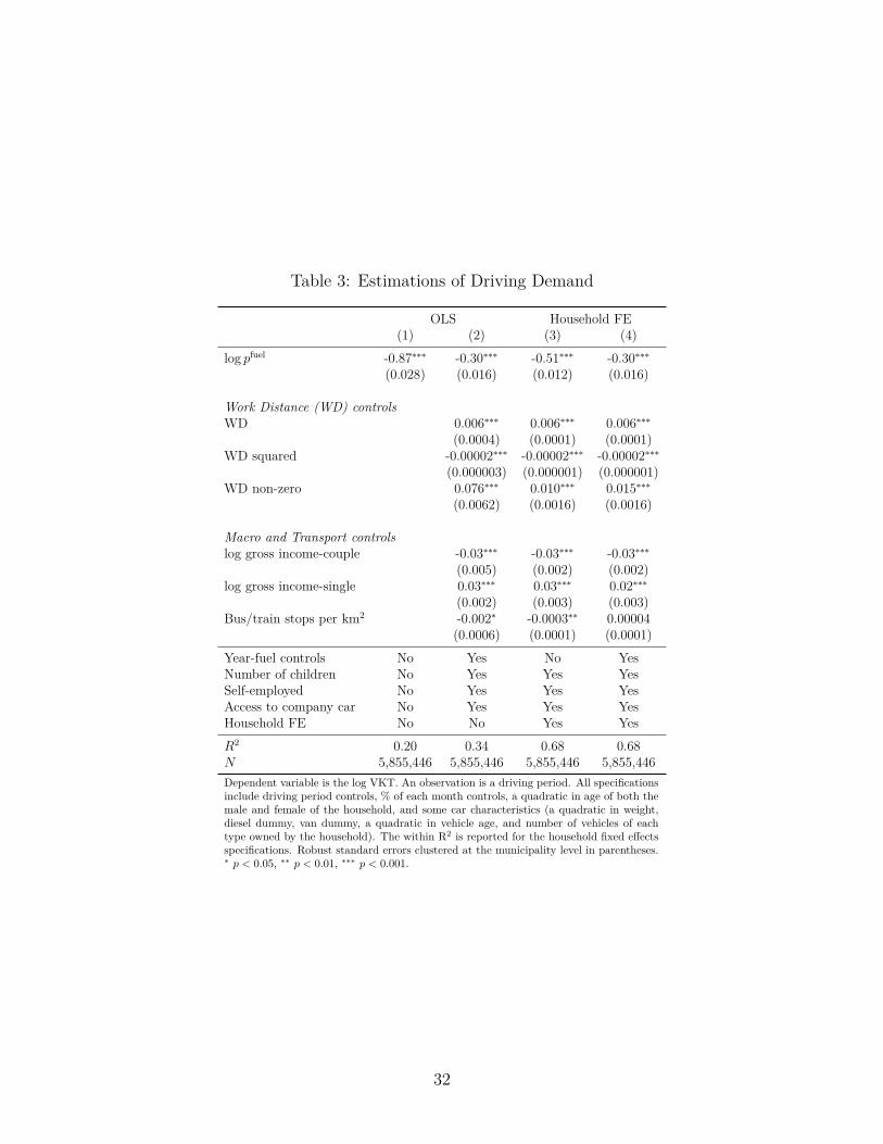
Table 3: Estimations of Driving Demand

OLS Household FE(1) (2) (3) (4)

log pfuel -0.87∗∗∗ -0.30∗∗∗ -0.51∗∗∗ -0.30∗∗∗(0.028) (0.016) (0.012) (0.016)

Work Distance (WD) controlsWD 0.006∗∗∗ 0.006∗∗∗ 0.006∗∗∗

(0.0004) (0.0001) (0.0001)WD squared -0.00002∗∗∗ -0.00002∗∗∗ -0.00002∗∗∗

(0.000003) (0.000001) (0.000001)WD non-zero 0.076∗∗∗ 0.010∗∗∗ 0.015∗∗∗

(0.0062) (0.0016) (0.0016)

Macro and Transport controlslog gross income-couple -0.03∗∗∗ -0.03∗∗∗ -0.03∗∗∗

(0.005) (0.002) (0.002)log gross income-single 0.03∗∗∗ 0.03∗∗∗ 0.02∗∗∗

(0.002) (0.003) (0.003)Bus/train stops per km2 -0.002∗ -0.0003∗∗ 0.00004

(0.0006) (0.0001) (0.0001)Year-fuel controls No Yes No YesNumber of children No Yes Yes YesSelf-employed No Yes Yes YesAccess to company car No Yes Yes YesHousehold FE No No Yes YesR2 0.20 0.34 0.68 0.68N 5,855,446 5,855,446 5,855,446 5,855,446Dependent variable is the log VKT. An observation is a driving period. All specificationsinclude driving period controls, % of each month controls, a quadratic in age of both themale and female of the household, and some car characteristics (a quadratic in weight,diesel dummy, van dummy, a quadratic in vehicle age, and number of vehicles of eachtype owned by the household). The within R2 is reported for the household fixed effectsspecifications. Robust standard errors clustered at the municipality level in parentheses.∗ p < 0.05, ∗∗ p < 0.01, ∗∗∗ p < 0.001.

32

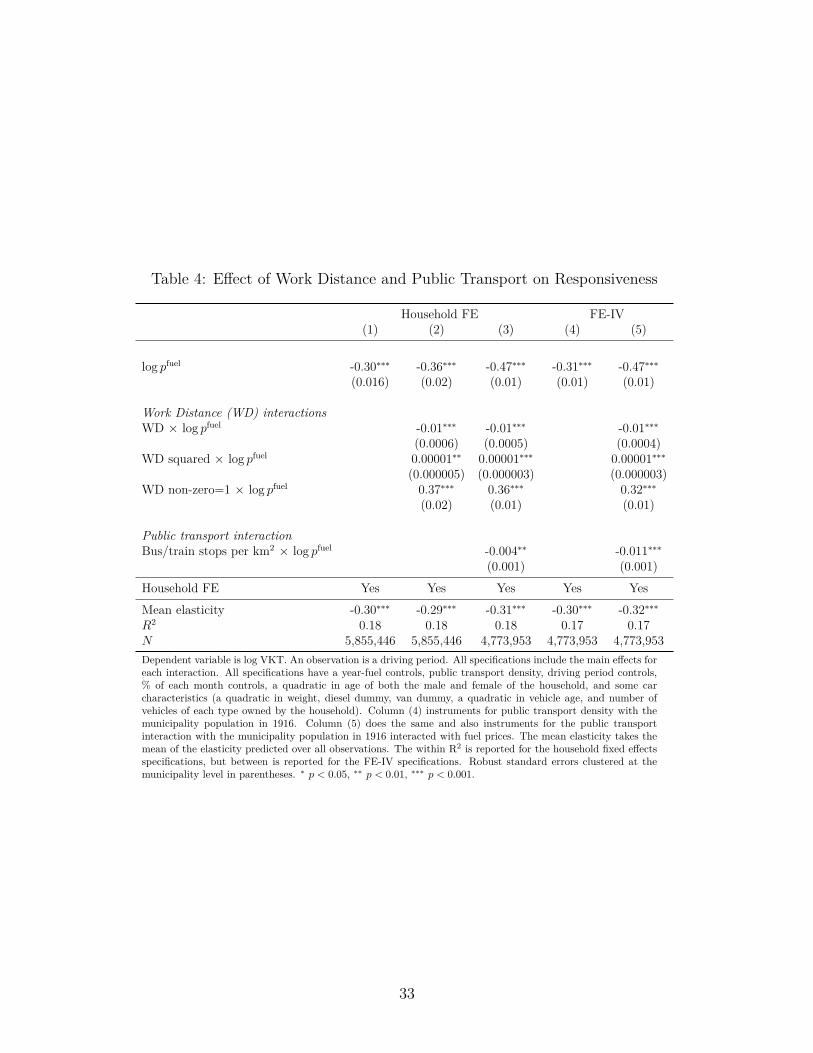
Table 4: Effect of Work Distance and Public Transport on Responsiveness

Household FE FE-IV(1) (2) (3) (4) (5)

log pfuel -0.30∗∗∗ -0.36∗∗∗ -0.47∗∗∗ -0.31∗∗∗ -0.47∗∗∗(0.016) (0.02) (0.01) (0.01) (0.01)

Work Distance (WD) interactionsWD × log pfuel -0.01∗∗∗ -0.01∗∗∗ -0.01∗∗∗

(0.0006) (0.0005) (0.0004)WD squared × log pfuel 0.00001∗∗ 0.00001∗∗∗ 0.00001∗∗∗

(0.000005) (0.000003) (0.000003)WD non-zero=1 × log pfuel 0.37∗∗∗ 0.36∗∗∗ 0.32∗∗∗

(0.02) (0.01) (0.01)

Public transport interactionBus/train stops per km2 × log pfuel -0.004∗∗ -0.011∗∗∗

(0.001) (0.001)Household FE Yes Yes Yes Yes YesMean elasticity -0.30∗∗∗ -0.29∗∗∗ -0.31∗∗∗ -0.30∗∗∗ -0.32∗∗∗R2 0.18 0.18 0.18 0.17 0.17N 5,855,446 5,855,446 4,773,953 4,773,953 4,773,953Dependent variable is log VKT. An observation is a driving period. All specifications include the main effects foreach interaction. All specifications have a year-fuel controls, public transport density, driving period controls,% of each month controls, a quadratic in age of both the male and female of the household, and some carcharacteristics (a quadratic in weight, diesel dummy, van dummy, a quadratic in vehicle age, and number ofvehicles of each type owned by the household). Column (4) instruments for public transport density with themunicipality population in 1916. Column (5) does the same and also instruments for the public transportinteraction with the municipality population in 1916 interacted with fuel prices. The mean elasticity takes themean of the elasticity predicted over all observations. The within R2 is reported for the household fixed effectsspecifications, but between is reported for the FE-IV specifications. Robust standard errors clustered at themunicipality level in parentheses. ∗ p < 0.05, ∗∗ p < 0.01, ∗∗∗ p < 0.001.

33

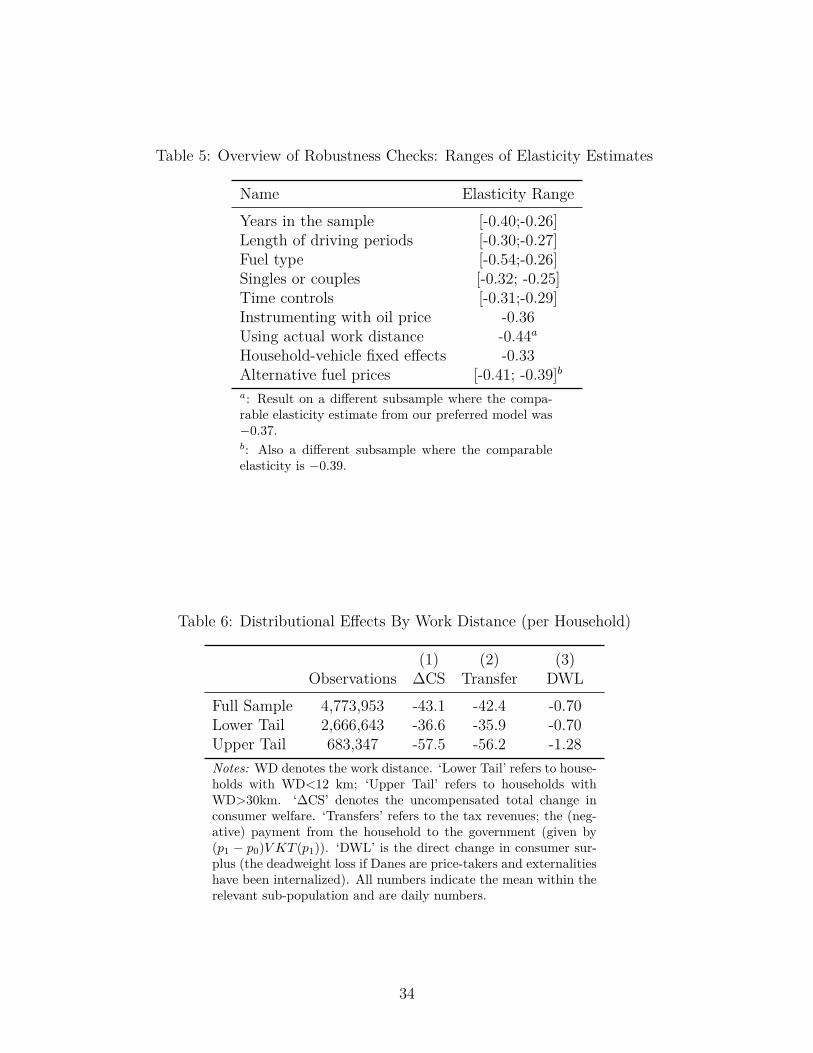
Table 5: Overview of Robustness Checks: Ranges of Elasticity Estimates

Name Elasticity RangeYears in the sample [-0.40;-0.26]Length of driving periods [-0.30;-0.27]Fuel type [-0.54;-0.26]Singles or couples [-0.32; -0.25]Time controls [-0.31;-0.29]Instrumenting with oil price -0.36Using actual work distance -0.44aHousehold-vehicle fixed effects -0.33Alternative fuel prices [-0.41; -0.39]ba: Result on a different subsample where the compa-rable elasticity estimate from our preferred model was−0.37.b: Also a different subsample where the comparableelasticity is −0.39.

Table 6: Distributional Effects By Work Distance (per Household)

(1) (2) (3)Observations ∆CS Transfer DWL

Full Sample 4,773,953 -43.1 -42.4 -0.70Lower Tail 2,666,643 -36.6 -35.9 -0.70Upper Tail 683,347 -57.5 -56.2 -1.28Notes: WD denotes the work distance. ‘Lower Tail’ refers to house-holds with WD<12 km; ‘Upper Tail’ refers to households withWD>30km. ‘∆CS’ denotes the uncompensated total change inconsumer welfare. ‘Transfers’ refers to the tax revenues; the (neg-ative) payment from the household to the government (given by(p1 − p0)V KT (p1)). ‘DWL’ is the direct change in consumer sur-plus (the deadweight loss if Danes are price-takers and externalitieshave been internalized). All numbers indicate the mean within therelevant sub-population and are daily numbers.

34

Figures

Figure 1: Vehicle Kilometers Traveled (VKT) and Fuel Price

(a) Levels

88

.59

9.5

20

05

DK

K p

er

lite

r fu

el

44

46

48

50

52

VK

T

1998 2001 2003 2006 2009Start date of period

VKT Fuel price

Note: Local polynomial average smoothed by start date.

(b) Logarithms

2.1

2.15

2.2

2.25

log

2005

DKK

per

lite

r fue

l

3.55

3.6

3.65

3.7

3.75

VKT

(log)

1998 2001 2003 2006 2009Start date of period

VKT Fuel priceNote: Local polynomial average smoothed by start date.

Figure 2: Percentiles of Driving Over Time

(a) VKT

050

100

150

200

VKT

1998 2000 2002 2004 2006Start-year of driving period

P1 P5 P10 P25 P50P75 P90 P95 P99 Mean

Percentiles of VKT Over Time

(b) log VKT

12

34

5lo

g VK

T

1998 2000 2002 2004 2006Start-year of driving period

P1 P5 P10 P25 P50P75 P90 P95 P99 log(mean)

Percentiles of VKT Over Time

35

Figure 3: Nonparametric Relationship Between Driving and Work Distance

4050

6070

Vehi

cle

kilo

met

ers

trave

led

(km

/day

)

0 20 40 60 80 100Work distance (km)

Mean driving 95% CI (clustered)

Notes: The line shows raw means within bins of work distance. We have split work distance according to 40bins with equally many observations, except for the zero bin (which holds half of observations). To constructthe confidence interval, we regressed driving on dummies for all bins, excluding a constant in the regression.We then used the standard errors (clustered at the municipality level) for these dummies to construct the95% confidence intervals around the means, multiplying by ±1.96. There are bins for work distance between0 and 12 due to households that work part time but have work distances above 12 km.

Figure 4: Average Work Distance by Municipality (Panel (a)) and Public Transport Stops(Panel (b))

(b)

CopenhagenCopenhagen

(a)

Copenhagen

36

Figure 5: Nonparametric Demand Curve

3.64

83.

653.

652

3.65

4lo

g VK

T (re

sidu

aliz

ed)

2.16 2.18 2.2 2.22 2.24log fuel price (residualized)

95% CI Demand

Note: This figure is constructed by first residualizing log VKT and log fuel price and then running alocal polynomial regression with the default bandwidth in Stata. The first-stage residualization is done byregressing the variable on a full set of controls (excluding the fuel price) and household fixed effects andextracting the residual. We show the relationship for residualized log fuel prices between the 1st and 99thpercentile of log fuel prices (2.15 and 2.24).

37

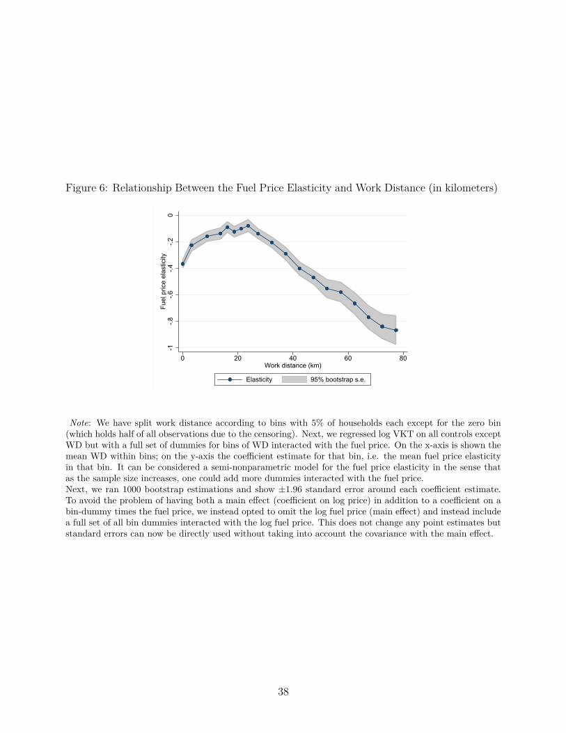
Figure 6: Relationship Between the Fuel Price Elasticity and Work Distance (in kilometers)-1

-.8-.6

-.4-.2

0Fu

el p

rice

elas

ticity

0 20 40 60 80Work distance (km)

Elasticity 95% bootstrap s.e.

Note: We have split work distance according to bins with 5% of households each except for the zero bin(which holds half of all observations due to the censoring). Next, we regressed log VKT on all controls exceptWD but with a full set of dummies for bins of WD interacted with the fuel price. On the x-axis is shown themean WD within bins; on the y-axis the coefficient estimate for that bin, i.e. the mean fuel price elasticityin that bin. It can be considered a semi-nonparametric model for the fuel price elasticity in the sense thatas the sample size increases, one could add more dummies interacted with the fuel price.Next, we ran 1000 bootstrap estimations and show ±1.96 standard error around each coefficient estimate.To avoid the problem of having both a main effect (coefficient on log price) in addition to a coefficient on abin-dummy times the fuel price, we instead opted to omit the log fuel price (main effect) and instead includea full set of all bin dummies interacted with the log fuel price. This does not change any point estimates butstandard errors can now be directly used without taking into account the covariance with the main effect.

38

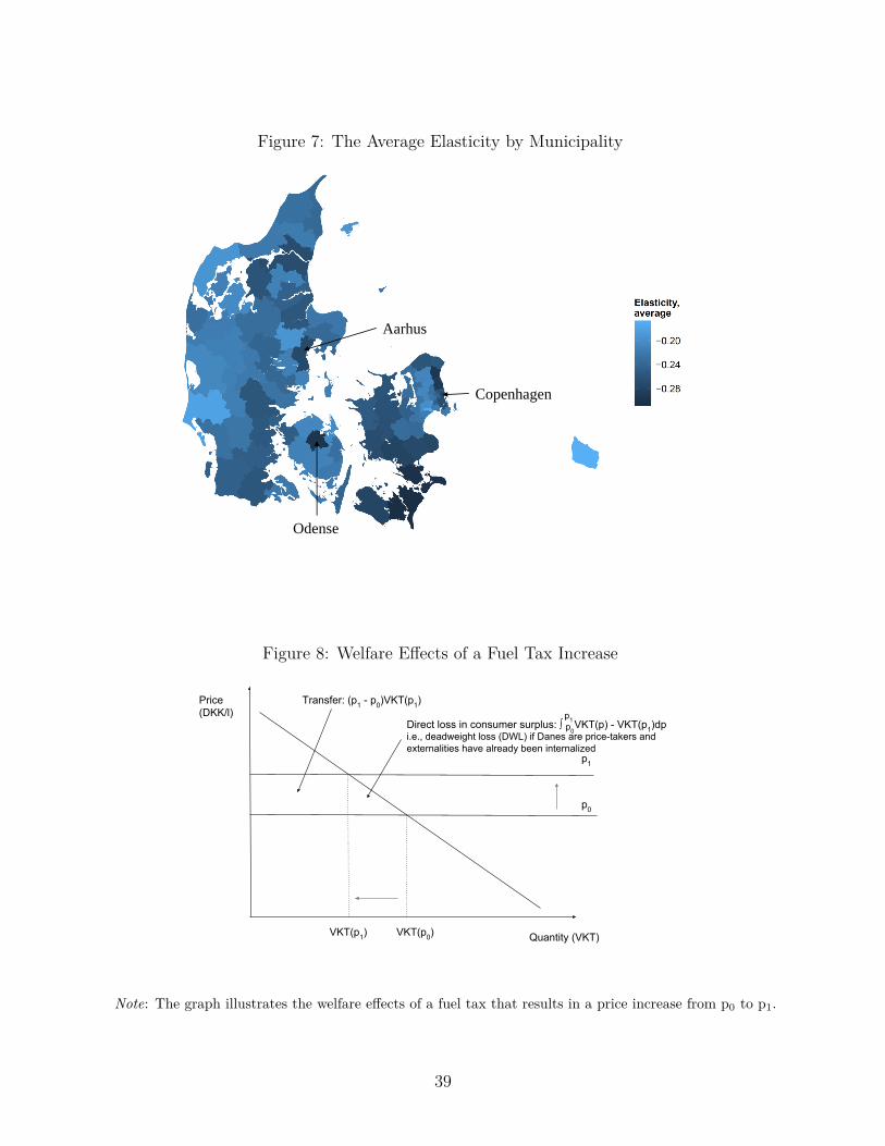
Figure 7: The Average Elasticity by Municipality

Copenhagen

Odense

Aarhus

Figure 8: Welfare Effects of a Fuel Tax Increase

Price(DKK/l)

Quantity (VKT)

p0

p1

VKT(p1) VKT(p0)

Transfer: (p1 - p0)VKT(p1)

Direct loss in consumer surplus: ∫ VKT(p) - VKT(p1)dpi.e., deadweight loss (DWL) if Danes are price-takers and externalities have already been internalized

p1p0

Note: The graph illustrates the welfare effects of a fuel tax that results in a price increase from p0 to p1.

39

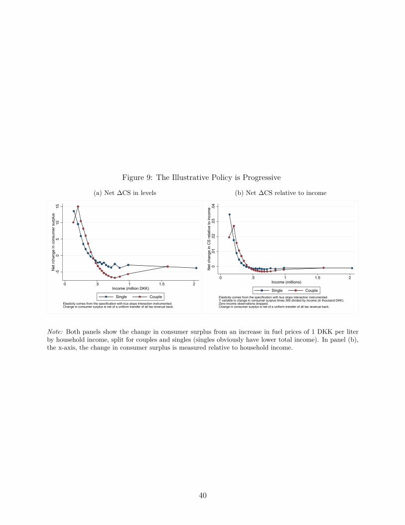
Figure 9: The Illustrative Policy is Progressive

(a) Net ∆CS in levels

-50

510

15N

et rc

hang

e in

con

sum

er s

urpl

us

0 .5 1 1.5 2Income (million DKK)

Single CoupleElasticity comes from the specification with bus stops interaction instrumented.Change in consumer surplus is net of a uniform transfer of all tax revenue back.

(b) Net ∆CS relative to income

0.0

1.0

2.0

3.0

4N

et c

hang

e in

CS

rela

tive

to in

com

e

0 .5 1 1.5 2Income (millions)

Single CoupleElasticity comes from the specification with bus stops interaction instrumented.Y variable is change in consumer surplus times 365 divided by income (in thousand DKK).Zero-income observations dropped.Change in consumer surplus is net of a uniform transfer of all tax revenue back.

Note: Both panels show the change in consumer surplus from an increase in fuel prices of 1 DKK per literby household income, split for couples and singles (singles obviously have lower total income). In panel (b),the x-axis, the change in consumer surplus is measured relative to household income.

40

ONLINE APPENDIX

A Data Appendix

Given the comprehensiveness and richness of the dataset used in this study, we include thisonline appendix to describe the data in more detail and elaborate on the sample selection.

A.1 Development of the Final Dataset

As a general rule, we focused our data cleaning efforts on avoiding dropping observationsto maximize our dataset coverage. Our data cleaning proceeded as follows. First, we con-verted the dataset into one where the observation is a driving period and all negative drivingobservations or other observations with critical missing data are dropped. This dataset has10,994,333 observations. We further restrict the data to have driving periods that beganafter July 1, 1998 (since tests were not mandatory prior to this date) and before January 1,2008 (this ensures that our sample is not biased away from new vehicles). These restrictionsleave us with 7,254,893 observations. After this, we delete observations where the lengthof the driving period, which we call years to test, is not either between 1 and 2.5 years orbetween 3.5 and 4.5 years. This is chosen to balance not getting too many observations withunexplained lengths of the driving periods while also accounting for early phase-in, whichled to a number of 1-year periods in 1999 and 2000. This leaves us with 6,877,185 drivingperiods. We have missing demographic variables for 277,294 observations, which brings usto 6,599,891 observations. We drop 178 outlier observations with VKT greater than 10,000km/day. Finally, because we use household fixed effects, we drop 744,267 households thatare only observed once in the dataset. This brings us to our final sample size of 5,855,446.

To clarify how these observations are distributed over time, Table 10 shows a histogramof the start year of the driving period. The low number in the first year is due to the sampleselection criterion keeping only periods starting after July 1, 1998.

The following sections provide more detail on the sources and cleaning of the data.

A.1.1 Car Ownership

The data we use on car ownership comes from the Danish Central Motor Register. Thisregister contains the license plate, vehicle identification number (VIN), and personal identi-fication number (i.e., CPR numbers, which allow us to merge these data in with other publicregisters). In the raw data, we observe some problematic observations. When we observea car with a car ownership period for one owner that does not end and a car ownership

41

Figure 10: Observations by start year

02

00

40

06

00

80

0O

bse

rva

tio

ns (

tho

usa

nd

s)

1998 2000 2002 2004 2006Start year of driving period

period for a different owner at a later date, we know that the transaction was not properlyrecorded. In this case, we assign the ending of the ownership period for the first owner at thedate when the second owner is first observed with the vehicle. We also do the same for thereverse scenario. We also occasionally see problematic observations where there is an overlapof owners. In that case, we have no way of discerning which person truly owns the car andaccording to the data documentation such an observation should be impossible so we dropthem from the dataset.

A.1.2 Driving Periods

The data on driving periods come from the Ministry of Transportation (MOT) tests thatwere introduced in 1997. These inspections are mandatory and must be performed at carages 4, 6, 8, 10, 12, etc. This means that we have two types of driving periods; The firstdriving period is 4 years long (that is, it has 4 years to test) and any subsequent drivingperiod will be only 2 years long. The inspection date is set based on the date of the firstregistration of the car in Denmark. In practice, the years to test may deviate with plus orminus three months around these designated years. A person may choose to take the car infor inspection earlier than the set date if he or she wishes.

MOT tests were originally performed by public authorities directly but in more recentyears, they have been performed by private companies approved by the MOT. The goal ofthe test is to verify that the car is in safe condition for driving on the roads. As a part ofthe test, the odometer of the car is recorded. A test may have four outcomes; 1) The car can

42

be approved. 2) The car can be conditionally approved, meaning that certain repairs mustbe performed for the car to be in legal driving order but that no extra test will be required.3) The car can be approved after a re-inspection, implying that repairs must be made andthen the car must return for another test before 33 calendar days. Finally, 4) the car canbe declared not approved in which case it will be illegal to drive the car and the police willwithdraw the license plates. Some drivers may take their vehicle in for an inspection earlyprior to selling the car in order to give the buyer a signal that the car is in proper workingorder. Figure 11 shows the distribution of the driving period length. The vertical lines markthe sample selection described above.

Figure 11: Years to Test Distribution

0.5

11

.5D

en

sity

0 2 4 6 8Test length in years

Note: Deselects observations with length over 8 years (9964 obs.).Vertical lines mark sample selection for estimation.

Driving period length

Note: Years to test is the time between two odometer readings. New cars come in for inspection around 4years and used cars around 2 years.

The sample selection criteria mentioned above for the timing of the driving periods canalso be seen in Figure 12. We have selected the sample for a period when the years to test isrelatively constant, thus helping to alleviate any concerns of sample selection bias based onthis variable.

A.2 Detailed Variable Description

Table 7 lists of all the variables used in this paper with details on each.

Table 7: Variables used in the paper

Variable Description

43

VKT Vehicle-kilometers-traveled in km per day. The variable is constructed by taking first-differencesof the odometer readings from the dataset with vehicle inspections. For the first inspection weobserve for a car, we assume that the odometer was zero at the time of the car’s first registrationin Denmark. This will be incorrect if the car was imported from abroad. However, then the carmust have had a toll inspection, which we observe, so we can run a robustness check on thisassumption. We find that this does not impact our results.

Couple Dummy for there being two members of the household (married or co-habiting, of oppositegenders and having at less than 15 years of age difference).

Real gross income The sum of gross incomes for the member(s) of the household. The variable comes from theincome tax registers. The variable includes all government transfers such as pension payments,unemployment benefits, etc.

Real gross income (couples) As above but equal to zero for singles.

Real gross income (singles) As above but equal to zero for couples.

WD Work distance. The variable is based on the Danish deduction for work distance. Any workinghousehold having further than 12 km each way to work can deduct a fixed amount per km.Thus, the measure will be equal to zero if the individual lives closer than 12 km from his orher work. Between 12 and 25 km, there is a rate and above 25 km, the rate drops to half.The rate changes over the period. The total deduction is the daily rate times the number ofdays worked. The variable is self-reported but the tax authorities have access to both the homeand work addresses for the individual. The deduction is the rate times the distance times thenumber of days worked. We do not observe the number of days worked so we assume 225 workdays, which corresponds to the number of days in a typical Danish work year. For example, theofficial number of work days were 224 in 2007, 226 in 2008, 225 in 2009 and 228 in 2010. Mostunions follows these, as do most public sector employees. Figure 16 shows the density of thework distance variable. Note that there is a positive mass on the interval (0; 12) km even thoughthe deduction is only given if the door-to-door work distance is above 12 km; this is due to theassumption about 225 work days per year. If an individual works part-time, say 110 days, buthas a distance of 20 km to work, then the variable will be equal to 10. The positive mass willtherefore contain many part time employees. For validity, we can compare it to the continuousWD measure, available for a subset of the period (see Appendix A.3.3).

WD non-zero Dummy for the WD measure being observed. Thus, this is essentially a dummy for the individualliving further than 12 km from the work place.

WD (door-to-door distance) This is the door-to-door distance from home to work. The variable comes from the DanishTechnical University’s Department of Transportation. It is calculated using a shortest-pathalgorithm and the National Transport model with GIS data on households and their work places.The variable is only observed for households where the work place is observed and not for 1998or 1999. In total, it is observed for 76.17% of our estimation sample (79.61% of the observationsbetween 2000 and 2008). We use this measure to validate the tax-based WD variable.

# of children The number of children aged less than 18 years living with the household.

Urban (dummy) Dummy equal to one if the household lives in either Copenhagen, Frederiksberg, Aarhus, Aalborgog Odense municipalities, which constitute the major Danish urban areas.

Company car Dummy equal to one if at least one member of the household has paid the tax penalty for havingaccess to a company car. The use of company cars is restricted to avoid making it an alternativeto buying your own car privately. The size of the tax depends on the value of the car. Wecollapse the variable to a dummy for having any car available to any of the members of thehousehold. Individuals may have access to a company car and not pay this tax if the car is a“yellow license plate” car. These cars can have at most two seats and are typically vans used bycraftsmen. The police enforce this very strictly and an individual caught using a company carprivately and not paying the penalty is fined and some times forced to pay the registration tax.

44

Self employed Dummy equal to one if the household has at least one self employed individual. This informationcomes from the tax registers.

# of periods observed The number of driving periods observed for the household. Note that the other driving periodsmay be with different cars and that our sample selects only households with at least two drivingperiods.

Bus/Train stops per km2 The number of public transport stops in the municipality in 2013 divided by the area of themunicipality of residence at the start of the driving period in km2. The data for this comes fromthe Travel Planner (http://rejseplanen.dk), which is a search engine for planning trips usingpublic transportation. The data are only available for a cross-section in 2013. The highest num-ber of stops is 79.9 stops per km2 for Odense municipality and the lowest is Aaskov municipalitywith 0.3 stops per km2.

Weight (ton) The gross weight of the car in metric tonnes. This is the maximum allowed weight of the vehicleincluding cargo. The variable comes from the vehicle type approval documents.

Diesel Dummy equal to one if the car uses diesel fuel. Note that the fuel price will then be based onthe diesel price.

Van Dummy equal to one if the vehicle is a van.

Percent owned of period The fraction of the driving period where the car was owned by this household. That is, if thedriving period starts on Jan 1st, 2001 and ends on Jan 1st 2003, but the car changed owner onJan 1st 2002, this variable will be equal to 0.5 for both the observations of the two householdsdriving the car.

Driving period length The length of the driving period in years. For new cars, this will be 4 years and for older cars,it will be 2 years, both plus or minus 3 months and with some exceptions. Note that our sampleselects on driving periods being either 1.0 to 2.5 years long or 3.5 to 4.5 years long.

Car age Car age in years at the start of the driving period. Car age is defined as the time since the car’sfirst registration in Denmark since we do not observe the actual production year of the vehicle.This will be very close to the number of years since the model year for most vehicles, but willbe off for the small number of imported vehicles.

# cars / vans / motorcycles /mopeds / trailers owned

Continuous measure of the number of vehicles of the given type owned by the household. Forexample, if for a given household i and driving period t, the household owns another car forthe entire duration of the period, then # of cars owned will be 2.0. If that other car is onlypurchased half-way through the driving period t, then it is equal to 1.5. That is, the variable isequal to the fraction of this driving period overlapping with the ownership of other vehicles.

First driving period Dummy equal to one if it is the car’s first driving period, i.e., the driving period’s start date isequal to the first registration date of the car.

Fraction owned For household i and driving period t, this is the percent of the driving period where houseohld iis the owner. That is, if the car changes owner midway through, there will be an observation inthe dataset for each of the two households owning the car and they will both have this variableset to 0.5.

Years to test The length of the driving period in years (continuous variable). Due to our sample selection,this will be in [1.0; 2.5] or in [3.5; 4.5].

% of each month This is a set of variables for each month equal to the % of the driving period taking place ineach of the 12 months. Thus, if a driving period is precisely 2 or 4 years long, these will all beequal to 1

12 . We omit April as the reference group in regressions since the fractions will alwayssum to 1.

Year controls These are variables for each year, 1998, ..., 2011, each equal to the % of the driving periodfalling in that year. In the preferred specification, we exclude year 2003 as the reference yearand include an additional full set of year controls interacted with the diesel dummy to allow aseparate time trend for diesels.

45

A.3 Additional Descriptives

A.3.1 Driving and Demographics

Figure 13 shows the distribution of vehicles kilometers traveled (VKT). The figure is cut at200 km/day for clarity. Note that there is still positive mass for very low VKT. This may beexplained by vehicles such as vintage or specialty cars.

A.3.2 Additional Spatial Descriptives

Figure 14 shows the number of observations (i.e., driving periods) by municipality. The fourmajor urban areas clearly stand out: Copenhagen (east), Odense (center, on the island ofFyn), Aarhus (midway up on the eastern side of Jutland) and Aalborg (Northern part ofJutland).

Figure 15 shows a map of Denmark where municipalities are colored by the average VKTof the households. We see that the households with high driving tend to be in the outskirts ofthe major urban areas with a few exceptions. Note that this figure plots observations in theestimation sample, so it should be interpreted recognizing that it conditions on householdsowning a car. Note that the car ownership rate is 40% in the five largest urban municipalitiesand 67% elsewhere in Denmark, so a map of the per capita driving would show even lowerdriving in the urban areas relative to rural areas.

A.3.3 Work Distance

In this subsection, we discuss the validity of the work distance variable. Table 8 showssummary statistics for work distances of males, females and singles. It shows both themeasure based on the tax deduction for work distance as well as the “door-to-door workdistance” variable, which measures the distance using GPS coordinates. The tax deductionis a deduction from taxable income and it is given as a fixed amount per kilometer per daybut is equal to zero if the distance is shorter than 12 km. The number of days worked is notobserved so we assume that all individuals work 225 days a year, which is very common inDenmark. Hence, if the individual actually worked fewer days, we will be undershooting themeasure (which explains why the variable can take values below 12 km) and vice versa. Theper km rate varies over time and there is a kink in the schedule at 50 km where it falls tohalf the rate.34

34In some years, a small number of fringe municipalities (Danish: udkantskommuner) also had the full rateafter the 50 km threshold.

46

Figure 12: Years to Test by Start Date of the Driving Period

23

45

6Y

ears

to test

1992 1994 1996 1998 2000 2002 2004 2006 2008 2010 2012Start date of driving period

Vertical lines mark January 1st 1994 and July 1st 1998 respectively.

Years to test by start of the driving period

Note: Years to test is the difference between two odometer readings. Since there are more used than new cars,the average is closer to 2 than 4. We start our sampling period in mid 1998 because the average stabilizeshere. Prior to that, cars were coming in that had never been to an inspection before and therefore had verylong driving periods.

To explore the validity of the work distance variable, we exploit the aforementioned door-to-door work distance, which is based on the address of the home and work location. Thus,it directly captures the literal work distance. However, it is not available for the full sampleand it is a massive over-estimate for households that work from home or work elsewhere thanthe primary office of their work. Thus, we see it as a useful robustness check and opt to usethe tax return variable in our primary specification.

We compare the distribution of driving according to the two variables to validate the taxreturn measure. To make the comparison sensible, make the comparison for the subsamplewhere both measures fall in the range [12 km ; 100 km]. The lower bound ensures that thetax-based measure is also observed, while the upper bound makes the graph easier to read.Figure 16 shows the comparison, demonstrating the comparability of the two work distancevariables.

47

Figure 13: The Distribution of Vehicle Kilometers Traveled

0.0

05.0

1.0

15.0

2D

ensi

ty

0 50 100 150 200Vehicle Kilometers Traveled

Note: Observations with more than 200km/day omitted.

Figure 14: Observations in the Estimation Sample by Municipality

50000

100000

150000

200000

250000Observations

48

Figure 15: Average Driving by Municipality

35

40

45

50

VKT,average

Table 8: Work Distance (WD) Variables

N mean sd p1 p10 p25 p50 p75 p90 p95 p99WD, male 4550411 9.5932 18.51 0.0 0.0 0.0 0.0 15.5 32.2 44.7 80.7WD, female 4550411 6.9385 13.77 0.0 0.0 0.0 0.0 10.7 24.8 33.7 58.3WD, single 1305035 7.6966 16.87 0.0 0.0 0.0 0.0 9.0 27.5 39.3 75.1WD non-zero, male 4550411 0.3493 0.48 0 0 0 0 1 1 1 1WD non-zero, female 4550411 0.3137 0.46 0 0 0 0 1 1 1 1WD non-zero, single 1305035 0.2917 0.45 0 0 0 0 1 1 1 1WD, door-to-door, male 3343884 20.3157 34.36 0.0 0.0 2.7 9.8 23.7 46.5 71.8 196.3WD, door-to-door, female 3094025 14.3657 22.45 0.0 0.6 2.8 8.1 18.1 32.1 45.0 99.3WD, door-to-door, single 813453 18.6009 32.87 0.0 0.1 2.6 8.6 21.1 42.0 66.1 183.4

Note: WD refers to the work distance variable based on the travel tax deduction, which is censored at 12 kmbut contains information on the number of days commuted. “WD door-to-door” refers to the shortest pathmeasure from home to work. The two measures should only be expected to be equal if the person has longerthan 12 km to work and works precisely 225 days each year.

49

Figure 16: Comparing the Two Work Distance Measures

0.0

1.0

2.0

3.0

4

20 40 60 80 100Work distance (male)

WD WD (actual)

Selection: males’ work distance should be in [12; 100] km with both measures (1013011 obs.).WD is based on the tax deduction and WD (actual) on GPS coordinates.

Note: Both curves are non-parametric kernel density estimates for the work distance for households where itis greater than 12 km for both measures. The tax-based measure features a few notable excess-mass points,which is most likely due to individuals rounding off if in doubt.

B Additional Regression Results

This appendix contains number of econometric results supplementing the primary resultsfrom section 4. To begin, Table 9 shows the coefficients pertaining to car characteristics andthe driving period that were suppressed in the primary results table in our paper.

To further explore heterogeneity, Table 10 shows the coefficients for the demographicvariables for the quantiles 1, 50 and 99 in the panel quantile regression estimates. They showthat many of the coefficients do not vary over the conditional distribution of VKT. However,the fuel price elasticity, work distance, company car dummy, and transit stop density variableschange.

50

Table 9: Main results — Car and Period Controls

OLS Household FE(1) (2) (3) (4)

No demo Base FE Mainlog pfuel -0.866∗∗∗ -0.298∗∗∗ -0.515∗∗∗ -0.304∗∗∗

(0.00509) (0.0143) (0.00722) (0.0154)New car -0.00350∗ 0.0128∗∗∗ 0.00838∗∗∗ 0.0394∗∗∗

(0.00148) (0.00148) (0.00160) (0.00164)Percent owned of period -0.189∗∗∗ -0.112∗∗∗ -0.0537∗∗∗ -0.0154∗∗∗

(0.000826) (0.000862) (0.00106) (0.00110)Driving period length -0.0507∗∗∗ -0.0541∗∗∗ -0.0465∗∗∗ -0.0242∗∗∗

(0.000634) (0.000645) (0.000681) (0.000725)Weight (ton) 0.00214∗∗∗ 0.00169∗∗∗ 0.00166∗∗∗ 0.00167∗∗∗

(0.00000523) (0.00000506) (0.00000799) (0.00000798)Weight squared -0.000000471∗∗∗ -0.000000369∗∗∗ -0.000000354∗∗∗ -0.000000354∗∗∗

(1.35e-09) (1.30e-09) (2.00e-09) (2.00e-09)Diesel 0.316∗∗∗ 0.311∗∗∗ 0.228∗∗∗ 0.259∗∗∗

(0.000918) (0.00557) (0.00139) (0.00545)Van -0.236∗∗∗ -0.199∗∗∗ -0.204∗∗∗ -0.205∗∗∗

(0.00117) (0.00115) (0.00171) (0.00170)Car age -0.0302∗∗∗ -0.0275∗∗∗ -0.0284∗∗∗ -0.0293∗∗∗

(0.0000932) (0.0000911) (0.000140) (0.000141)# cars owned 0.0482∗∗∗ -0.0202∗∗∗ -0.0581∗∗∗ -0.0501∗∗∗

(0.000593) (0.000759) (0.00114) (0.00109)# vans owned 0.0111∗∗∗ -0.0470∗∗∗ -0.0711∗∗∗ -0.0654∗∗∗

(0.00124) (0.00122) (0.00183) (0.00179)# motorcycles owned 0.0319∗∗∗ -0.00420∗∗∗ 0.0102∗∗∗ 0.0118∗∗∗

(0.00101) (0.000905) (0.00178) (0.00178)# mopeds owned 0.136∗∗∗ 0.0415∗∗∗ 0.0232∗∗∗ 0.0204∗∗∗

(0.00138) (0.00131) (0.00218) (0.00217)# trailers owned 0.0123∗∗∗ 0.0258∗∗∗ 0.00334∗∗ 0.00595∗∗∗

(0.000519) (0.000983) (0.00106) (0.00106)Year controls No Yes No YesHousehold FE No No Yes YesR2 0.20 0.34 0.68 0.68N 5,855,446 5,855,446 5,855,446 5,855,446Dependent variable is the log VKT. An observation is a driving period. All specifica-tions have all of the other variables and controls in Table 9. Robust standard errorsclustered at the household level in parentheses. ∗ p < 0.05, ∗∗ p < 0.01, ∗∗∗ p < 0.001.

51

Table 10: Panel Quantile Regression for P01, P50 and P99: Demographics

(1) (2) (3) (4)Linear P01 P50 P99

log pfuel -0.304∗∗∗ -0.559∗∗∗ -0.233∗∗∗ -0.609∗∗∗(0.0154) (0.0663) (0.00739) (0.0592)

Work Distance (WD) controlsWD, male 0.00242∗∗∗ 0.00137∗∗∗ 0.00260∗∗∗ 0.00347∗∗∗

(0.0000336) (0.000106) (0.0000118) (0.0000947)WD non-zero, male 0.0329∗∗∗ 0.0797∗∗∗ 0.0320∗∗∗ -0.00688

(0.00107) (0.00427) (0.000476) (0.00382)WD, female 0.00303∗∗∗ 0.00245∗∗∗ 0.00328∗∗∗ 0.00338∗∗∗

(0.0000443) (0.000151) (0.0000168) (0.000135)WD non-zero, female 0.0257∗∗∗ 0.0950∗∗∗ 0.0247∗∗∗ -0.0327∗∗∗

(0.00111) (0.00461) (0.000513) (0.00412)WD, single 0.00419∗∗∗ 0.00360∗∗∗ 0.00448∗∗∗ 0.00562∗∗∗

(0.0000835) (0.000216) (0.0000241) (0.000193)WD non-zero, single 0.0724∗∗∗ 0.138∗∗∗ 0.0713∗∗∗ -0.0174∗

(0.00243) (0.00832) (0.000927) (0.00743)

Age controlsAge, male 0.0212∗∗ 0.0224∗∗∗ 0.0213∗∗∗ 0.0199∗∗∗

(0.00813) (0.00133) (0.000148) (0.00119)Age, female 0.0468∗∗∗ 0.0534∗∗∗ 0.0469∗∗∗ 0.0403∗∗∗

(0.00813) (0.00132) (0.000148) (0.00118)Age, single 0.0598∗∗∗ 0.0631∗∗∗ 0.0604∗∗∗ 0.0549∗∗∗

(0.000939) (0.000971) (0.000108) (0.000868)Age squared, male -0.0000930∗∗∗ -0.000118∗∗∗ -0.0000943∗∗∗ -0.0000705∗∗∗

(0.0000112) (0.0000128) (0.00000143) (0.0000115)Age squared, female -0.000195∗∗∗ -0.000275∗∗∗ -0.000197∗∗∗ -0.000117∗∗∗

(0.0000115) (0.0000134) (0.00000149) (0.0000120)Age squared, single -0.000206∗∗∗ -0.000275∗∗∗ -0.000213∗∗∗ -0.000119∗∗∗

(0.00000767) (0.00000933) (0.00000104) (0.00000834)

Other demographic controlslog gross inc (couple) -0.0242∗∗∗ -0.0156∗∗∗ -0.0176∗∗∗ -0.0278∗∗∗

(0.00162) (0.00304) (0.000339) (0.00272)log gross inc (single) 0.0200∗∗∗ 0.0268∗∗∗ 0.0195∗∗∗ 0.0144∗∗∗

(0.00288) (0.00226) (0.000252) (0.00202)Urban (dummy) -0.0249∗∗∗ -0.0392∗∗∗ -0.0254∗∗∗ -0.0146∗∗

(0.00284) (0.00519) (0.000578) (0.00463)# of kids -0.0168∗∗∗ -0.0145∗∗∗ -0.0169∗∗∗ -0.0145∗∗∗

(0.000650) (0.00146) (0.000163) (0.00130)Company car -0.0977∗∗∗ -0.312∗∗∗ -0.102∗∗∗ 0.0601∗∗∗

(0.00216) (0.00695) (0.000775) (0.00621)Self employed 0.000712 -0.0818∗∗∗ 0.00334∗∗∗ 0.0694∗∗∗

(0.00136) (0.00426) (0.000474) (0.00380)Bus/Train stops per km2 0.0000419 -0.0000421 0.0000173 0.000300∗∗

(0.0000548) (0.000103) (0.0000114) (0.0000916)

Year controls Yes Yes Yes Yes% of each month Yes Yes Yes YesCar Yes Yes Yes YesPeriod Yes Yes Yes YesLinear Fixed Effects (FE) Yes No No NoCanay (2011) FE No Yes Yes YesN 5855446 5855446 5855446 5855446Standard errors in parentheses. FE are at the household level.∗ p < 0.05, ∗∗ p < 0.01, ∗∗∗ p < 0.001

52

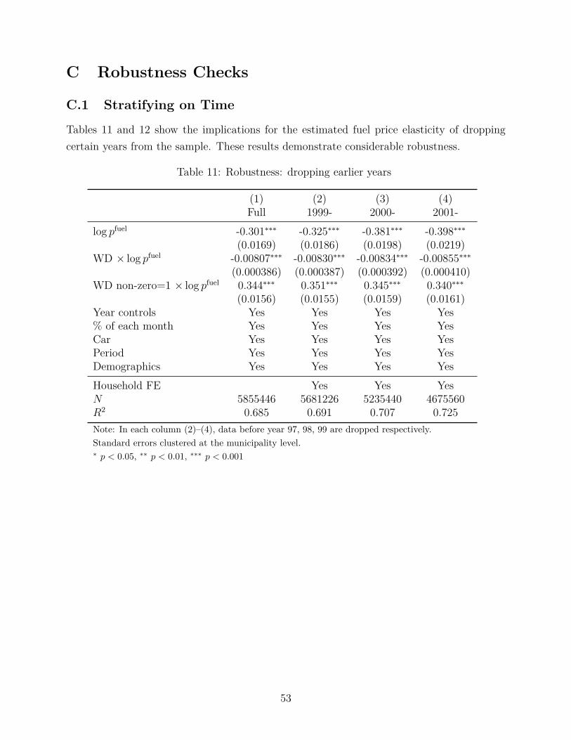
C Robustness Checks

C.1 Stratifying on Time

Tables 11 and 12 show the implications for the estimated fuel price elasticity of droppingcertain years from the sample. These results demonstrate considerable robustness.

Table 11: Robustness: dropping earlier years

(1) (2) (3) (4)Full 1999- 2000- 2001-

log pfuel -0.301∗∗∗ -0.325∗∗∗ -0.381∗∗∗ -0.398∗∗∗(0.0169) (0.0186) (0.0198) (0.0219)

WD × log pfuel -0.00807∗∗∗ -0.00830∗∗∗ -0.00834∗∗∗ -0.00855∗∗∗(0.000386) (0.000387) (0.000392) (0.000410)

WD non-zero=1 × log pfuel 0.344∗∗∗ 0.351∗∗∗ 0.345∗∗∗ 0.340∗∗∗(0.0156) (0.0155) (0.0159) (0.0161)

Year controls Yes Yes Yes Yes% of each month Yes Yes Yes YesCar Yes Yes Yes YesPeriod Yes Yes Yes YesDemographics Yes Yes Yes YesHousehold FE Yes Yes YesN 5855446 5681226 5235440 4675560R2 0.685 0.691 0.707 0.725Note: In each column (2)–(4), data before year 97, 98, 99 are dropped respectively.Standard errors clustered at the municipality level.∗ p < 0.05, ∗∗ p < 0.01, ∗∗∗ p < 0.001

53

Table 12: Robustness: dropping later years

(1) (2) (3) (4)Full -2006 -2005 -2004

log pfuel -0.301∗∗∗ -0.255∗∗∗ -0.307∗∗∗ -0.278∗∗∗(0.0169) (0.0186) (0.0191) (0.0198)

WD × log pfuel -0.00807∗∗∗ -0.00801∗∗∗ -0.00818∗∗∗ -0.00873∗∗∗(0.000386) (0.000403) (0.000408) (0.000506)

WD non-zero=1 × log pfuel 0.344∗∗∗ 0.335∗∗∗ 0.348∗∗∗ 0.347∗∗∗(0.0156) (0.0160) (0.0169) (0.0194)

Year controls Yes Yes Yes Yes% of each month Yes Yes Yes YesCar Yes Yes Yes YesPeriod Yes Yes Yes YesDemographics Yes Yes Yes YesHousehold FE Yes Yes YesN 5855446 5177147 4443035 3736630R2 0.685 0.697 0.712 0.727Note: In each column (2)–(4), data after year 06, 05, 04 are dropped respectively.Standard errors clustered at the municipality level.∗ p < 0.05, ∗∗ p < 0.01, ∗∗∗ p < 0.001

C.2 Stratifying on Couples or Singles

Table 13 shows the results when estimating on the sample consisting exclusively of couplesor singles, again demonstrating considerable robustness.

54

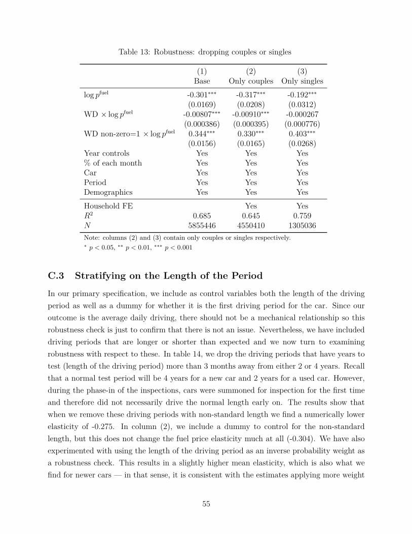
Table 13: Robustness: dropping couples or singles

(1) (2) (3)Base Only couples Only singles

log pfuel -0.301∗∗∗ -0.317∗∗∗ -0.192∗∗∗(0.0169) (0.0208) (0.0312)

WD × log pfuel -0.00807∗∗∗ -0.00910∗∗∗ -0.000267(0.000386) (0.000395) (0.000776)

WD non-zero=1 × log pfuel 0.344∗∗∗ 0.330∗∗∗ 0.403∗∗∗(0.0156) (0.0165) (0.0268)

Year controls Yes Yes Yes% of each month Yes Yes YesCar Yes Yes YesPeriod Yes Yes YesDemographics Yes Yes YesHousehold FE Yes YesR2 0.685 0.645 0.759N 5855446 4550410 1305036Note: columns (2) and (3) contain only couples or singles respectively.∗ p < 0.05, ∗∗ p < 0.01, ∗∗∗ p < 0.001

C.3 Stratifying on the Length of the Period

In our primary specification, we include as control variables both the length of the drivingperiod as well as a dummy for whether it is the first driving period for the car. Since ouroutcome is the average daily driving, there should not be a mechanical relationship so thisrobustness check is just to confirm that there is not an issue. Nevertheless, we have includeddriving periods that are longer or shorter than expected and we now turn to examiningrobustness with respect to these. In table 14, we drop the driving periods that have years totest (length of the driving period) more than 3 months away from either 2 or 4 years. Recallthat a normal test period will be 4 years for a new car and 2 years for a used car. However,during the phase-in of the inspections, cars were summoned for inspection for the first timeand therefore did not necessarily drive the normal length early on. The results show thatwhen we remove these driving periods with non-standard length we find a numerically lowerelasticity of -0.275. In column (2), we include a dummy to control for the non-standardlength, but this does not change the fuel price elasticity much at all (-0.304). We have alsoexperimented with using the length of the driving period as an inverse probability weight asa robustness check. This results in a slightly higher mean elasticity, which is also what wefind for newer cars — in that sense, it is consistent with the estimates applying more weight

55

to the newer driving observations.We have also experimented with a regression where we assign each observation a weight

proportional to the length of the driving period. We found that this raises the elasticity alittle, moving it towards the higher elasticity we find when we estimate on the subsample ofhouseholds holding newer cars.

Table 14: Robustness: length of the driving period

(1) (2) (3)Base Dummy Subsample

log pfuel -0.301∗∗∗ -0.296∗∗∗ -0.268∗∗∗(0.0169) (0.0172) (0.0187)

WD × log pfuel -0.00807∗∗∗ -0.00807∗∗∗ -0.00906∗∗∗(0.000386) (0.000386) (0.000412)

WD non-zero=1 × log pfuel 0.344∗∗∗ 0.344∗∗∗ 0.300∗∗∗(0.0156) (0.0157) (0.0151)

Non-standard test length -0.00274∗∗(0.000834)

Year controls Yes Yes Yes% of each month Yes Yes YesCar Yes Yes YesPeriod Yes Yes YesDemographics Yes Yes YesHousehold FE Yes Yes YesR2 0.685 0.685 0.726N 5855446 5855446 4535353Note: Standard test length: years to test is ± 3 months from either 2 or 4 years.Elsewhere, sample selection requires VKT in [1;2.5] or [3.5;4.5] years.Standard errors clustered at the municipality level.∗ p < 0.05, ∗∗ p < 0.01, ∗∗∗ p < 0.001

C.4 Year and Seasonality Controls

Table 15 shows the results when we change the way we control for time effects in decreasingcomplexity over the columns. The results show that even if we simplify down to a specificationwith only a linear time trend, our mean elasticity is nearly unchanged. However, if we removetime controls entirely, the elasticity changes substantially.

56

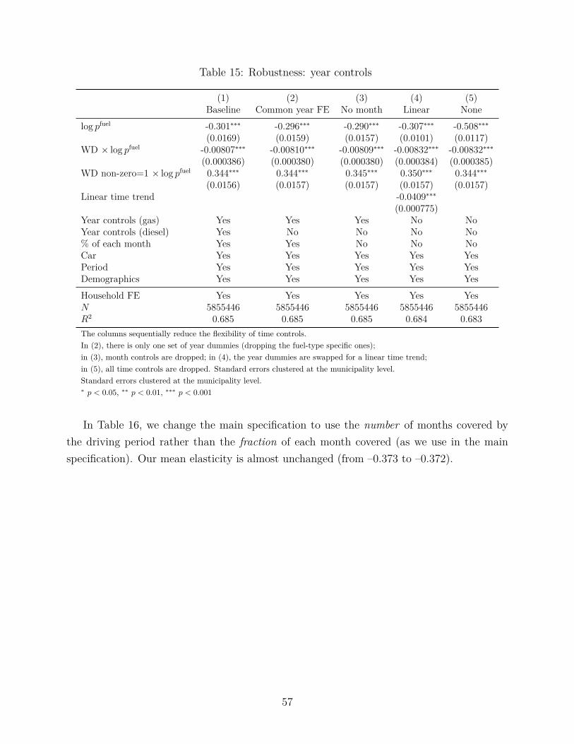
Table 15: Robustness: year controls

(1) (2) (3) (4) (5)Baseline Common year FE No month Linear None

log pfuel -0.301∗∗∗ -0.296∗∗∗ -0.290∗∗∗ -0.307∗∗∗ -0.508∗∗∗(0.0169) (0.0159) (0.0157) (0.0101) (0.0117)

WD × log pfuel -0.00807∗∗∗ -0.00810∗∗∗ -0.00809∗∗∗ -0.00832∗∗∗ -0.00832∗∗∗(0.000386) (0.000380) (0.000380) (0.000384) (0.000385)

WD non-zero=1 × log pfuel 0.344∗∗∗ 0.344∗∗∗ 0.345∗∗∗ 0.350∗∗∗ 0.344∗∗∗(0.0156) (0.0157) (0.0157) (0.0157) (0.0157)

Linear time trend -0.0409∗∗∗(0.000775)

Year controls (gas) Yes Yes Yes No NoYear controls (diesel) Yes No No No No% of each month Yes Yes No No NoCar Yes Yes Yes Yes YesPeriod Yes Yes Yes Yes YesDemographics Yes Yes Yes Yes YesHousehold FE Yes Yes Yes Yes YesN 5855446 5855446 5855446 5855446 5855446R2 0.685 0.685 0.685 0.684 0.683The columns sequentially reduce the flexibility of time controls.In (2), there is only one set of year dummies (dropping the fuel-type specific ones);in (3), month controls are dropped; in (4), the year dummies are swapped for a linear time trend;in (5), all time controls are dropped. Standard errors clustered at the municipality level.Standard errors clustered at the municipality level.∗ p < 0.05, ∗∗ p < 0.01, ∗∗∗ p < 0.001

In Table 16, we change the main specification to use the number of months covered bythe driving period rather than the fraction of each month covered (as we use in the mainspecification). Our mean elasticity is almost unchanged (from –0.373 to –0.372).

57

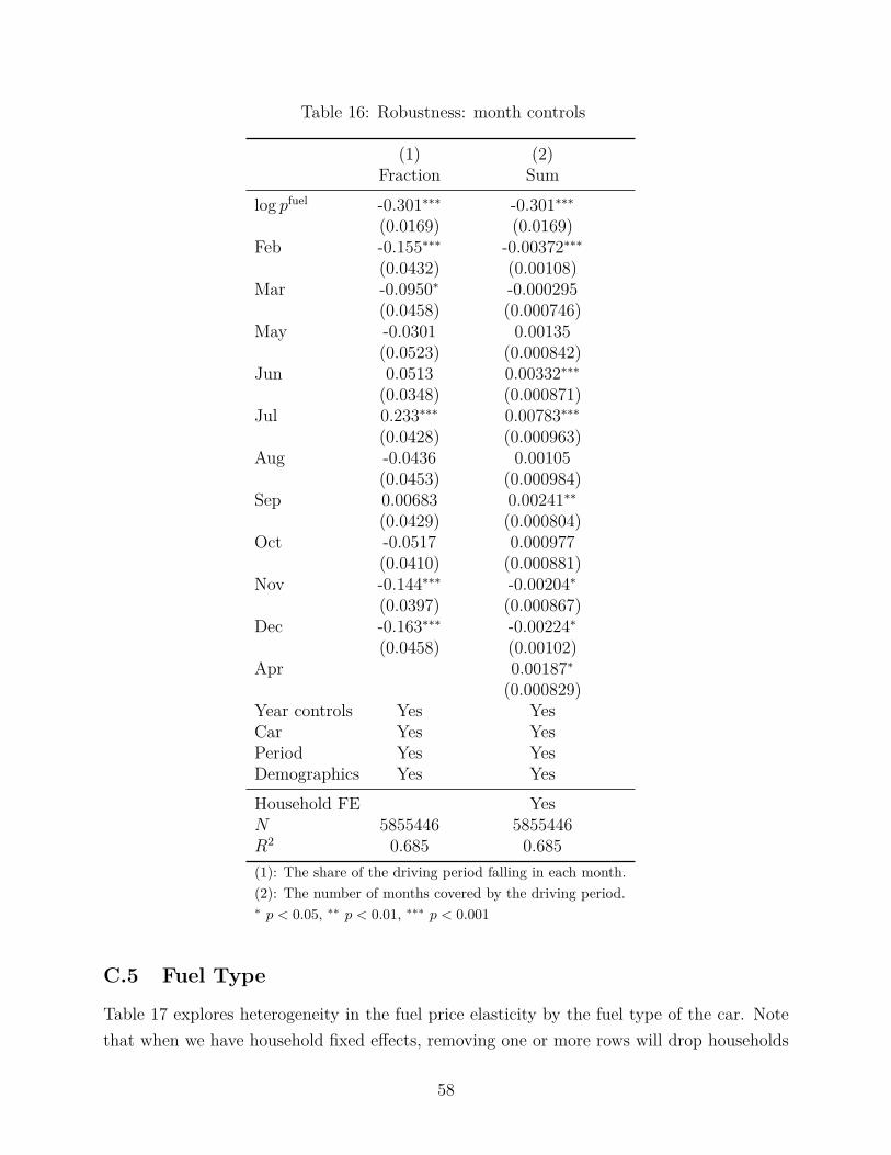
Table 16: Robustness: month controls

(1) (2)Fraction Sum

log pfuel -0.301∗∗∗ -0.301∗∗∗(0.0169) (0.0169)

Feb -0.155∗∗∗ -0.00372∗∗∗(0.0432) (0.00108)

Mar -0.0950∗ -0.000295(0.0458) (0.000746)

May -0.0301 0.00135(0.0523) (0.000842)

Jun 0.0513 0.00332∗∗∗(0.0348) (0.000871)

Jul 0.233∗∗∗ 0.00783∗∗∗(0.0428) (0.000963)

Aug -0.0436 0.00105(0.0453) (0.000984)

Sep 0.00683 0.00241∗∗(0.0429) (0.000804)

Oct -0.0517 0.000977(0.0410) (0.000881)

Nov -0.144∗∗∗ -0.00204∗(0.0397) (0.000867)

Dec -0.163∗∗∗ -0.00224∗(0.0458) (0.00102)

Apr 0.00187∗(0.000829)

Year controls Yes YesCar Yes YesPeriod Yes YesDemographics Yes YesHousehold FE YesN 5855446 5855446R2 0.685 0.685(1): The share of the driving period falling in each month.(2): The number of months covered by the driving period.∗ p < 0.05, ∗∗ p < 0.01, ∗∗∗ p < 0.001

C.5 Fuel Type

Table 17 explores heterogeneity in the fuel price elasticity by the fuel type of the car. Notethat when we have household fixed effects, removing one or more rows will drop households

58

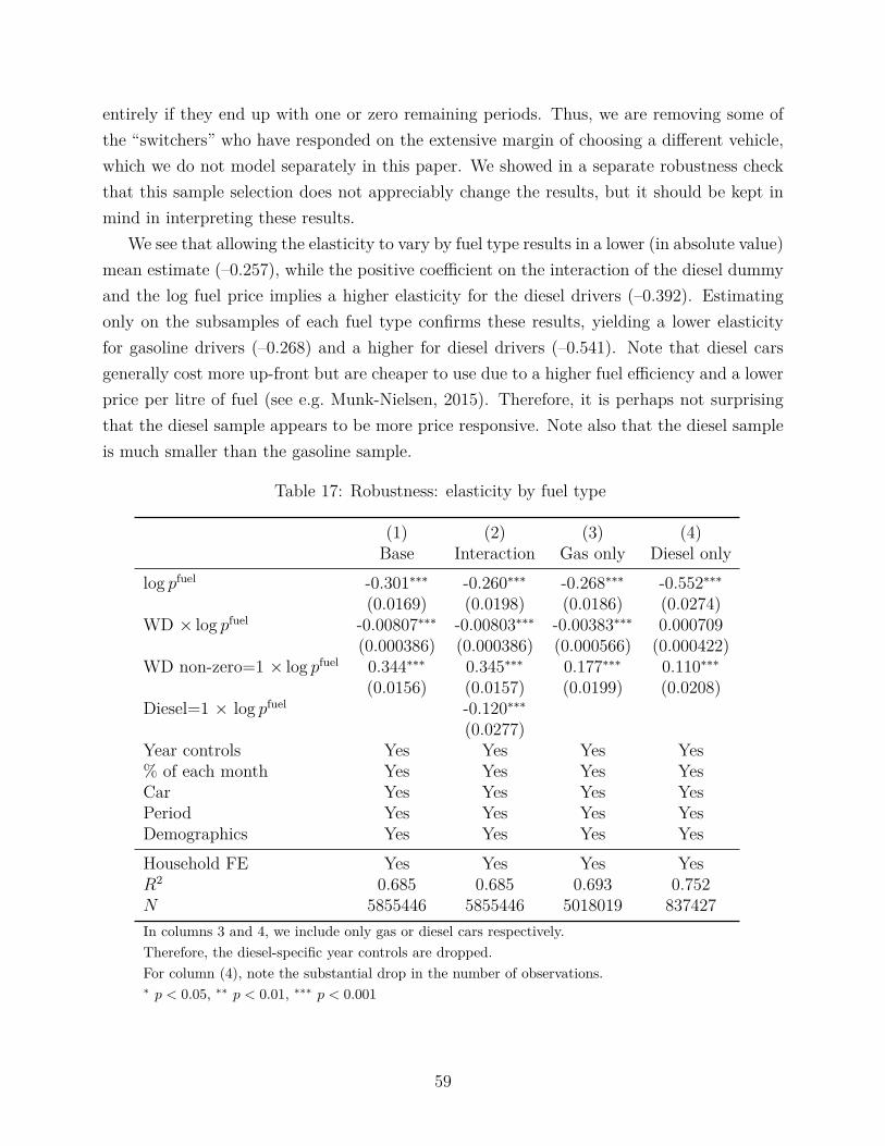
entirely if they end up with one or zero remaining periods. Thus, we are removing some ofthe “switchers” who have responded on the extensive margin of choosing a different vehicle,which we do not model separately in this paper. We showed in a separate robustness checkthat this sample selection does not appreciably change the results, but it should be kept inmind in interpreting these results.

We see that allowing the elasticity to vary by fuel type results in a lower (in absolute value)mean estimate (–0.257), while the positive coefficient on the interaction of the diesel dummyand the log fuel price implies a higher elasticity for the diesel drivers (–0.392). Estimatingonly on the subsamples of each fuel type confirms these results, yielding a lower elasticityfor gasoline drivers (–0.268) and a higher for diesel drivers (–0.541). Note that diesel carsgenerally cost more up-front but are cheaper to use due to a higher fuel efficiency and a lowerprice per litre of fuel (see e.g. Munk-Nielsen, 2015). Therefore, it is perhaps not surprisingthat the diesel sample appears to be more price responsive. Note also that the diesel sampleis much smaller than the gasoline sample.

Table 17: Robustness: elasticity by fuel type

(1) (2) (3) (4)Base Interaction Gas only Diesel only

log pfuel -0.301∗∗∗ -0.260∗∗∗ -0.268∗∗∗ -0.552∗∗∗(0.0169) (0.0198) (0.0186) (0.0274)

WD × log pfuel -0.00807∗∗∗ -0.00803∗∗∗ -0.00383∗∗∗ 0.000709(0.000386) (0.000386) (0.000566) (0.000422)

WD non-zero=1 × log pfuel 0.344∗∗∗ 0.345∗∗∗ 0.177∗∗∗ 0.110∗∗∗(0.0156) (0.0157) (0.0199) (0.0208)

Diesel=1 × log pfuel -0.120∗∗∗(0.0277)

Year controls Yes Yes Yes Yes% of each month Yes Yes Yes YesCar Yes Yes Yes YesPeriod Yes Yes Yes YesDemographics Yes Yes Yes YesHousehold FE Yes Yes Yes YesR2 0.685 0.685 0.693 0.752N 5855446 5855446 5018019 837427In columns 3 and 4, we include only gas or diesel cars respectively.Therefore, the diesel-specific year controls are dropped.For column (4), note the substantial drop in the number of observations.∗ p < 0.05, ∗∗ p < 0.01, ∗∗∗ p < 0.001

59

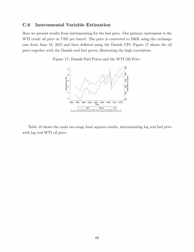
C.6 Instrumental Variable Estimation

Here we present results from instrumenting for the fuel price. Our primary instrument is theWTI crude oil price in USD per barrel. The price is converted to DKK using the exchangerate from June 18, 2015 and then deflated using the Danish CPI. Figure 17 shows the oilprice together with the Danish real fuel prices, illustrating the high correlation.

Figure 17: Danish Fuel Prices and the WTI Oil Price

10

02

00

30

04

00

50

06

00

20

05

DK

K p

er

ba

rre

l

67

89

10

11

20

05

DK

K p

er

lite

r

1996 1998 2000 2002 2004 2006 2008 2010 2012Date

O95 Diesel Oil

Oil price is converted with the spot USD to DKK rate and then deflated by Danish CPI

Table 18 shows the main two-stage least squares results, instrumenting log real fuel pricewith log real WTI oil price.

60

Table 18: Instrumental Variables Results

No FE FE(1) (2) (3) (4)

OLS 2SLS FE 2SLS FElog pfuel -0.298∗∗∗ -0.484∗∗∗ -0.301∗∗∗ -0.364∗∗∗

(0.0177) (0.0221) (0.0169) (0.0244)WD × log pfuel -0.00548∗∗∗ -0.000544 -0.00807∗∗∗ -0.000336

(0.000611) (0.000691) (0.000386) (0.000471)WD non-zero=1 × log pfuel 0.404∗∗∗ -0.205∗∗∗ 0.344∗∗∗ 0.121∗∗∗

(0.0235) (0.0248) (0.0156) (0.0196)Year controls Yes Yes Yes Yes% of each month Yes Yes Yes YesCar Yes Yes Yes YesPeriod Yes Yes Yes YesDemographics Yes Yes Yes YesHousehold FE No No YesN 5855446 5855331 5855446 5855296Standard errors in parentheses∗ p < 0.05, ∗∗ p < 0.01, ∗∗∗ p < 0.001

Table 19 shows the first stage results. Note that the very high R2 of 98% is partially dueto the fact that overlapping periods are repeated. These results indicate that the log oil priceis a very strong instrument. The F-statistic for both columns is well above 100.

Table 19: Instrumental Variables Results: First Stage

(1) (2)Simple Full

-0.973∗∗∗ -0.855∗∗∗(0.000299) (0.000700)

log poil 0.176∗∗∗ 0.177∗∗∗(0.0000187) (0.0000552)

1(Dieselcar)× log poil 0.147∗∗∗ 0.124∗∗∗(0.0000519) (0.000129)

All controls No YesHousehold FE No NoN 5855331 5855331R2 0.972 0.982Standard errors in parentheses∗ p < 0.05, ∗∗ p < 0.01, ∗∗∗ p < 0.001

61

C.7 Fuel Efficiency and Car Price

In this section, we argue why our estimate of the fuel price elasticity is not biased by ourinclusion of most, but not all, vehicle characteristics. First, we show that adding the fueleconomy as a control (in the subsample where the variable is observed) does not change thefuel price elasticity.

In Table 20, we show the results of our primary estimation only including fuel economyand car price (manufacturer’s suggested retail price, MSRP). One major reason why thesevariables are not included in the main specifications is that they are only available for asubset of the period. The data source for these variables is the Danish Automobile DealerAssociation (DAF). This dataset has been merged to the VINs used by the Motor Register.35

The results in Table 20 show how the sample where the characteristics are observed isdifferent from the estimation sample used throughout this paper; switching to this subsamplechanges the fuel price elasticity from –0.30 to –0.59 (see column (2)). This can be at leastpartly explained by there being more households with newer cars in the subsample; from theinteraction results, we saw that households who have newer cars tend to also be more pricesensitive. Including the fuel efficiency variable in column (3) only very slightly changes theelasticity from -0.59 to -0.58. Further including the MSRP in column (4) leaves this almostentirely unchanged (-0.58). We take this as an indication that the included car characteristicsare so highly correlated with these variables, that we have little to worry about by excludingthem.

35The authors gratefully acknowledge Ismir Mulalic at DTU Transport for his assistance with this.

62

Table 20: Robustness: controlling for fuel efficiency and MSRP

(1) (2) (3) (4)Base Subsample Add km/l Add MSRP

log pfuel -0.301∗∗∗ -0.602∗∗∗ -0.593∗∗∗ -0.594∗∗∗(0.0169) (0.0220) (0.0219) (0.0222)

Fuel efficiency in km/l -0.00246∗∗∗ 0.00167∗∗∗(0.000508) (0.000452)

Car price 0.000000477∗∗∗(1.55e-08)

WD × log pfuel -0.00807∗∗∗ -0.00504∗∗∗ -0.00503∗∗∗ -0.00516∗∗∗(0.000386) (0.000415) (0.000415) (0.000408)

WD non-zero=1 × log pfuel 0.344∗∗∗ 0.437∗∗∗ 0.436∗∗∗ 0.430∗∗∗(0.0156) (0.0174) (0.0174) (0.0169)

Weight (ton) 0.00167∗∗∗ 0.00197∗∗∗ 0.00194∗∗∗ 0.00177∗∗∗(0.0000267) (0.0000282) (0.0000274) (0.0000305)

Weight squared -0.000000354∗∗∗ -0.000000385∗∗∗ -0.000000381∗∗∗ -0.000000366∗∗∗(5.48e-09) (5.62e-09) (5.61e-09) (6.21e-09)

Diesel 0.257∗∗∗ 0.217∗∗∗ 0.231∗∗∗ 0.198∗∗∗(0.00646) (0.00971) (0.0109) (0.0105)

Van -0.204∗∗∗ -0.230∗∗∗ -0.232∗∗∗ -0.137∗∗∗(0.00304) (0.00324) (0.00339) (0.00436)

Car age -0.0293∗∗∗ -0.0194∗∗∗ -0.0199∗∗∗ -0.0176∗∗∗(0.000413) (0.000298) (0.000297) (0.000306)

# cars owned -0.0498∗∗∗ -0.0258∗∗∗ -0.0258∗∗∗ -0.0270∗∗∗(0.00146) (0.00168) (0.00168) (0.00171)

# vans owned -0.0653∗∗∗ -0.0803∗∗∗ -0.0802∗∗∗ -0.0841∗∗∗(0.00188) (0.00241) (0.00240) (0.00247)

# motorcycles owned 0.0117∗∗∗ 0.00874∗∗∗ 0.00868∗∗∗ 0.00843∗∗∗(0.00172) (0.00213) (0.00212) (0.00211)

# mopeds owned 0.0210∗∗∗ 0.0167∗∗∗ 0.0167∗∗∗ 0.0168∗∗∗(0.00234) (0.00261) (0.00261) (0.00262)

# trailers owned 0.00592∗∗∗ 0.00870∗∗∗ 0.00866∗∗∗ 0.00876∗∗∗(0.00126) (0.00135) (0.00134) (0.00135)

Year controls Yes Yes Yes Yes% of each month Yes Yes Yes YesPeriod Yes Yes Yes YesDemographics Yes Yes Yes YesHousehold FE Yes Yes YesR2 0.685 0.779 0.779 0.780N 5855446 3035301 3035301 3035301(2), (3) and (4) restricts the sample to fuel efficiency and car MSRP being observed.∗ p < 0.05, ∗∗ p < 0.01, ∗∗∗ p < 0.001

C.8 Location Decisions and Work Distance

In this section, we address robustness with respect to household and firm location decisions.We have data on the home municipality of the household. This allows us to classify house-holds as moving based on whether they ever change municipality. Table 21 shows the key

63

specification estimated on the primary sample of 5.9m households and on the subsample of3.2m households make a move across municipal borders in column (2). The mean elasticity islarger, changing from -0.30 to -0.36, but all coefficients relating to the work distance and itsinteraction with the fuel price are not statistically different. This indicates that our findingof a different elasticity for households in the tails of the work distance distribution is notdriven by households relocating.

Next, we turn to the firm location decisions. In our data, we can identify the firm aworker is employed at as well as the individual sub-unit (“plant”) within the firm. Our datacontains information on whether the plant relocates in a given year. This information iscreated by Statistics Denmark based on the plant locations where individuals work.36 Asone might expect, relocations are not extremely common in our data, but common enoughto leave us with 49,074 household-driving-periods to estimate our model on.

In column (3), we estimate on the subsample of 49,074 households where the work locationof at least one spouse relocates. The 95% confidence intervals around these parameters allcontain the original parameter estimates. In column (4), we estimate only with householdswhere the firm did not relocate and the results are extremely close to the original results. Ofcourse, the spouse where the firm moves may decide to look for a different job in responseto advance information about the firm relocating. In columns (5) we only use the 26,803observations where the firm relocates but where the household does not and again, theoriginal parameter estimates are all contained in the 95% confidence interval. Finally, incolumn (6), we only estimate on the 3.2m households that moved but where neither spouseworked at a firm-plant that relocated. It almost does not change the results to exclude thehouseholds where the firm relocated.

36In their raw data, Statistics Denmark observes one address no longer being associated with a firm and anew one being, and they observe the addresses of many of the workers switching from the old address to thenew. They require a minimum of the workers from one location appearing at the new in order for it to beclassified as a relocation.

64

Table 21: Robustness: Stratifying on location choices

(1) (2) (3) (4) (5) (6)Baseline HH moves Firm moves Firm stays Firm, not HH HH, not firm

Estimation sample contains observations where:Household moves Yes Yes No Yes No YesHousehold never moves Yes No Yes Yes Yes NoFirm moves Yes Yes Yes No Yes NoFirms never moves Yes Yes No Yes No Yeslog pfuel -0.356∗∗∗ -0.418∗∗∗ -0.374∗ -0.357∗∗∗ -0.457∗ -0.416∗∗∗

(0.0200) (0.0223) (0.151) (0.0201) (0.208) (0.0223)WD 0.0270∗∗∗ 0.0233∗∗∗ 0.0426∗∗∗ 0.0269∗∗∗ 0.0509∗∗ 0.0231∗∗∗

(0.00135) (0.00209) (0.0110) (0.00136) (0.0155) (0.00209)WD non-zero -0.807∗∗∗ -0.769∗∗∗ -0.643∗ -0.808∗∗∗ -0.907∗ -0.767∗∗∗

(0.0376) (0.0570) (0.280) (0.0374) (0.435) (0.0564)WD × log pfuel -0.00980∗∗∗ -0.00800∗∗∗ -0.0172∗∗∗ -0.00974∗∗∗ -0.0204∗∗ -0.00794∗∗∗

(0.000634) (0.000964) (0.00490) (0.000641) (0.00710) (0.000965)WD non-zero=1 × log pfuel 0.374∗∗∗ 0.357∗∗∗ 0.310∗ 0.375∗∗∗ 0.421∗ 0.356∗∗∗

(0.0172) (0.0260) (0.126) (0.0171) (0.197) (0.0257)Mean elasticity -0.302 -0.355 -0.414 -0.302 -0.493 -0.352Household FE Yes Yes Yes Yes Yes YesN 5855446 3244793 49074 5806372 26803 3168183Standard errors clustered at the municipality-level in parentheses.A household is defined as “moving” if it is observed in two different municipalities. Households are assigned to firmsbased on their registered primary employer. We match households to the firm they work and to the individual worklocation within the firm they work (which we refer to as a “plant”). Our data contains information on whether theparticular plant relocated in a given year. If the plant relocates and the household still works with the firm in the yearof the relocation, we classify that entire household observation as one where the firm moves.∗ p < 0.05, ∗∗ p < 0.01, ∗∗∗ p < 0.001

C.9 Macro effects: unemployment and alternative fuels

Table 22 includes controls for unemployment. The data is based on uninsurance benefitsclaims and we use both a dummy for any unemployment during the driving period as wellas a measure of the fraction of the driving period covered by unemployment. Each of thesecontrols are specific by gender and single households.

65

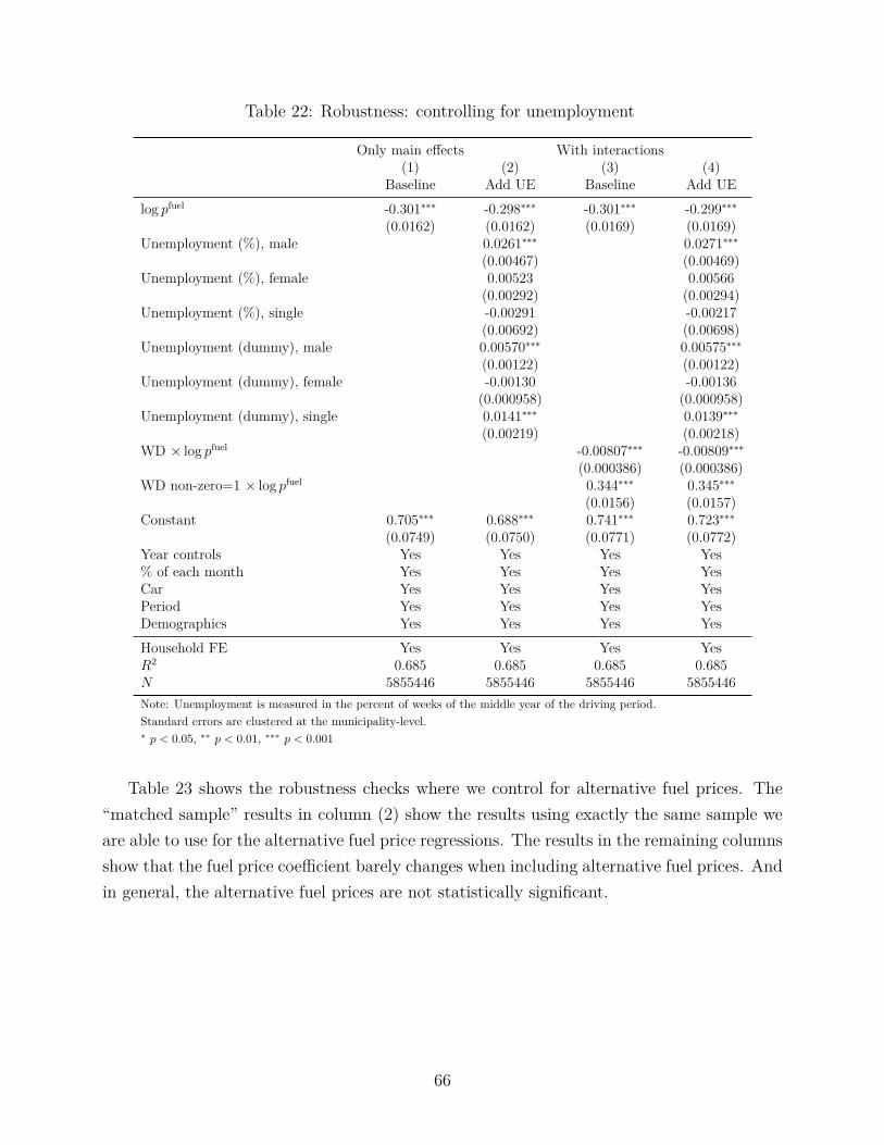
Table 22: Robustness: controlling for unemployment

Only main effects With interactions(1) (2) (3) (4)

Baseline Add UE Baseline Add UElog pfuel -0.301∗∗∗ -0.298∗∗∗ -0.301∗∗∗ -0.299∗∗∗

(0.0162) (0.0162) (0.0169) (0.0169)Unemployment (%), male 0.0261∗∗∗ 0.0271∗∗∗

(0.00467) (0.00469)Unemployment (%), female 0.00523 0.00566

(0.00292) (0.00294)Unemployment (%), single -0.00291 -0.00217

(0.00692) (0.00698)Unemployment (dummy), male 0.00570∗∗∗ 0.00575∗∗∗

(0.00122) (0.00122)Unemployment (dummy), female -0.00130 -0.00136

(0.000958) (0.000958)Unemployment (dummy), single 0.0141∗∗∗ 0.0139∗∗∗

(0.00219) (0.00218)WD × log pfuel -0.00807∗∗∗ -0.00809∗∗∗

(0.000386) (0.000386)WD non-zero=1 × log pfuel 0.344∗∗∗ 0.345∗∗∗

(0.0156) (0.0157)Constant 0.705∗∗∗ 0.688∗∗∗ 0.741∗∗∗ 0.723∗∗∗

(0.0749) (0.0750) (0.0771) (0.0772)Year controls Yes Yes Yes Yes% of each month Yes Yes Yes YesCar Yes Yes Yes YesPeriod Yes Yes Yes YesDemographics Yes Yes Yes YesHousehold FE Yes Yes Yes YesR2 0.685 0.685 0.685 0.685N 5855446 5855446 5855446 5855446Note: Unemployment is measured in the percent of weeks of the middle year of the driving period.Standard errors are clustered at the municipality-level.∗ p < 0.05, ∗∗ p < 0.01, ∗∗∗ p < 0.001

Table 23 shows the robustness checks where we control for alternative fuel prices. The“matched sample” results in column (2) show the results using exactly the same sample weare able to use for the alternative fuel price regressions. The results in the remaining columnsshow that the fuel price coefficient barely changes when including alternative fuel prices. Andin general, the alternative fuel prices are not statistically significant.

66

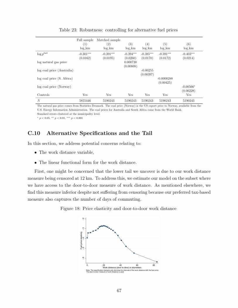
Table 23: Robustness: controlling for alternative fuel prices

Full sample Matched sample(1) (2) (3) (4) (5) (6)

log km log km log km log km log km log kmlog pfuel -0.301∗∗∗ -0.391∗∗∗ -0.394∗∗∗ -0.385∗∗∗ -0.391∗∗∗ -0.403∗∗∗

(0.0162) (0.0195) (0.0260) (0.0170) (0.0172) (0.0214)log natural gas price 0.000730

(0.00808)log coal price (Australia) -0.00255

(0.00397)log coal price (S. Africa) -0.0000288

(0.00425)log coal price (Norway) -0.00566∗

(0.00228)Controls Yes Yes Yes Yes Yes YesN 5855446 5190243 5190243 5190243 5190243 5190243The natural gas price comes from Statistics Denmark. The coal price (Norway) is the US export price to Norway, available from theU.S. Energy Information Administration. The coal prices for Australia and South Africa come from the World Bank.Standard errors clustered at the municipality level.∗ p < 0.05, ∗∗ p < 0.01, ∗∗∗ p < 0.001

C.10 Alternative Specifications and the Tail

In this section, we address potential concerns relating to:

• The work distance variable,

• The linear functional form for the work distance.

First, one might be concerned that the lower tail we uncover is due to our work distancemeasure being censored at 12 km. To address this, we estimate our model on the subset wherewe have access to the door-to-door measure of work distance. As mentioned elsewhere, wefind this measure inferior despite not suffering from censoring because our preferred tax-basedmeasure also captures the number of days of commuting.

Figure 18: Price elasticity and door-to-door work distance

-.6-.5

-.4-.3

-.2Fu

el p

rice

elas

ticity

0 20 40 60 80Work distance (door to door) in kilometers

Note: The specification interacts only dummies for intervals of the work distance with the fuel price.The door-to-door measure of work distance is used.

67

Second, we turn to the functional form for how the work distance enters. Omitting theother controls, our specification takes the form

log VKTit = (γ0 + γ1WDit + γ21{WDit>0}) log pfuelit + δ0 + δ1WDit + δ21{WDit>0} + · · ·

One may worry that our linear specification in work distance does not capture the truerelationship in the elasticity, or find it unnatural to have log in price and quantity but notwork distance. However, we find this to be the most natural specification because the workdistance–in contrast to the fuel price and driving–takes the value of zero often. Nevertheless,to satisfy the curious reader, Table 19 shows that the finding of a U-shape in the elasticityover work distance also arises from such a specification. We are presenting the results fromthe following regression:

log VKTit = (γ0+γ11{WDit>0} log WDit+γ21{WDit>0}) log pfuelit +δ0+δ11{WDit>0} log WDit+δ21{WDit>0}+· · ·

Figure 19 shows that the picture is qualitatively exactly the same as in the primary speci-fication, shown in Figure 6, although the functional form of the relationship now naturallydisplays slight additional curvature due to logarithic form in work distance.

Figure 19: Price elasticity work distance measured in logs

-.5-.4

-.3-.2

Pred

icte

d fu

el p

rice

elas

ticity

0 20 40 60 80 100Work distance

Note: The work distance is the maximum for couples. Horizontal line marks 12 km.Elasticity comes from the specification with log work distance.Elasticity is averaged within bins of work distance.

68

D A Simple Model of Travel Decisions

This section develops a simple model of the travel decision of a car-owning agent in order tobuild intuition for the economics underlying our empirical results. The focus of this model ison the economics of the short-run price responsiveness of driving and how it varies with thework distance of the household. For clarity of exposition, we abstract from other decisionsthat may influence driving in the long-run, such as where to live and what employment toaccept. Our model is well-suited for a setting where the decision-maker has access to publictransport. Such a setting is relevant to nearly all of Denmark, as well as much of Europeand many other areas in the world. For example, in 2014, 87% of Danes live within onekilometer of a public transport stop and nearly all the remainder are served by on-call buses(“telebusser”).37 We model a static setting for a given finite amount of time, such as oneweek.

Let the total number of kilometers traveled by the agent be given by T . The agent cantravel by personal vehicle or by other modes of transport, including public transport, biking,or walking. Let the kilometers traveled by personal vehicle be denoted by v, so the remainingkilometers traveled is T − v. Consider two types of travel. The first type is repeated travelthat occurs several times a week, such as for a commute to work. The second is discretionary,shopping, or leisure travel. Let dw ∈ [0, 1] be the fraction of commuting (work) trips driven.dw = 1 if all of commuting is accomplished by driving and dw = 0 if all of commuting isdone by other modes of transport. Similarly, let dl ∈ [0, 1] be the fraction for non-commuting(leisure) trips.

Let w be the kilometers traveled for the commute and gw(dw, w) be the additional utilityfrom commuting to work by driving rather than other forms of transport. Similarly, let l bethe kilometers traveled for non-work trips and gl(dl, l) be the utility from driving for non-work trips. In the short-run, w is not a choice variable, so gw(dw, w) ≡ gw(dw). In contrast,l is a choice variable. As driving is a more flexible form of transport, assume ∂gl(dw)

∂dw > 0 and∂gl(dl)∂dl > 0. However, there is an important difference between commuting trips and other

trips that motivates our specification of these functions. While trips for shopping or leisureinvolve travel to a diverse set of locations, commute trips are very homogenous, from thesame origin to the same destination and usually at the same time of day. Thus, for a givenset of commute trips in a given time period, we expect the marginal utility from commutingby personal car to be constant, regardless of the amount of driving. This allows us to define

37See http://passagerpulsen.taenk.dk/file/68/download?token=fy19yEeh, Accessed June 16, 2015.

69

gw(dw) ≡ γwdw, where γw is a constant.38 In contrast, there is inherent heterogeneity in theability to bike, walk, or take public transport for non-commute trips. For some shopping orleisure trips, public transport or biking are very attractive modes of travel; for others, theyare highly unappealing due to the distance or destination.

Consider an agent who maximizes utility subject to a budget constraint:

maxdw∈[0,1],dl∈[0,1],l

u(x) + gw(dw) + gl(dl, l)

s.t. y ≥ pvv + pb(T − v) + x,

where x is the outside good (whose price is normalized to 1), y is total income, pv is the priceper kilometer of driving a personal vehicle (hence “v”), and pb is the price per kilometer ofthe non-driving mode such as a bus (hence “b”).

Inserting the assumed form of gw, the Lagrangian for this problem can be written as

maxdw∈[0,1],dl∈[0,1],l

u(x) + γwdw + gl(dl, l) + λ[y − (pv − pb)v − pbT − x

],

where λ is the shadow price or marginal utility of income.Assuming standard regularity conditions and using v = dww + dll, the optimal dl can be

characterized by the following first-order condition:

∂g(dl, l)∂dl

= λ(pv − pb)l.

This condition indicates that the household will choose the fraction of non-commute driving,dl ∈ [0, 1], so that the marginal utility of an additional kilometer traveled by car is equal tothe marginal cost (converted to be in terms of utility). Because shopping and leisure tripsare heterogenous, the household will shift the least inconvenient trips to public transport,walking, or biking when fuel prices increase. Of course, corner solutions at 0 and 1 are possibleif the marginal cost is sufficiently high or low. Otherwise, ∂2gl(dl,l)

∂(dl)2 6= 0 and the monotonicityof gl(·) assures an interior solution, as one would expect. Similarly, the first order conditionfor l is ∂gl(dl,l)

∂l= λ

[(pv − pb)(dl − dw)− pb

], which indicates that the marginal benefits of

additional non-commute driving are equal to the marginal costs.The setting is different for commuting, as ∂gw(dw)

∂dw = γw. Given this, as long as we do nothave exact indifference (i.e., γw = λ(pv − pb)w), a utility-maximizing household would neverchoose an interior solution. Instead, we obtain the following discrete solution for the choice

38This follows from the short-run nature of the decision. In the longer-run, the utility from the workcommute may be increasing in w, as it may allow for the household to buy a better house or get a betterjob. But in the short-run, the house and job are fixed and thus the utility from commuting is fixed.

70

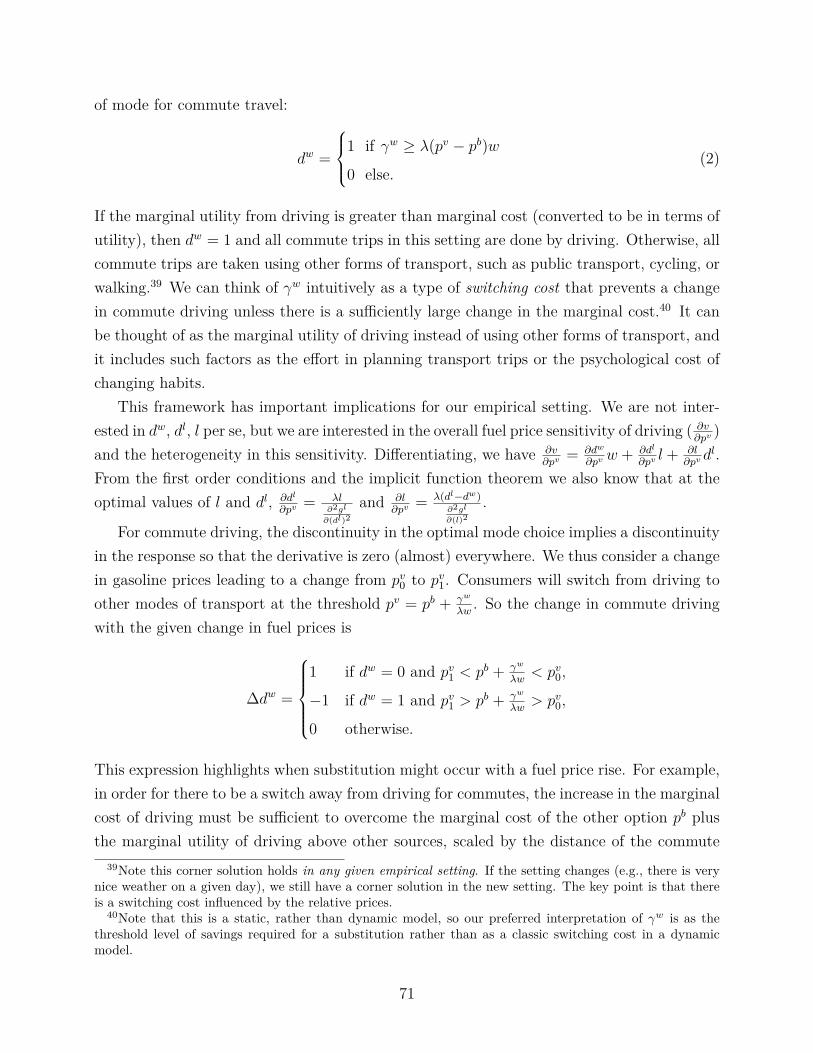
of mode for commute travel:

dw =

1 if γw ≥ λ(pv − pb)w

0 else.(2)

If the marginal utility from driving is greater than marginal cost (converted to be in terms ofutility), then dw = 1 and all commute trips in this setting are done by driving. Otherwise, allcommute trips are taken using other forms of transport, such as public transport, cycling, orwalking.39 We can think of γw intuitively as a type of switching cost that prevents a changein commute driving unless there is a sufficiently large change in the marginal cost.40 It canbe thought of as the marginal utility of driving instead of using other forms of transport, andit includes such factors as the effort in planning transport trips or the psychological cost ofchanging habits.

This framework has important implications for our empirical setting. We are not inter-ested in dw, dl, l per se, but we are interested in the overall fuel price sensitivity of driving ( ∂v

∂pv )and the heterogeneity in this sensitivity. Differentiating, we have ∂v

∂pv = ∂dw

∂pv w + ∂dl

∂pv l + ∂l∂pv d

l.From the first order conditions and the implicit function theorem we also know that at theoptimal values of l and dl, ∂dl

∂pv = λl∂2gl

∂(dl)2and ∂l

∂pv = λ(dl−dw)∂2gl

∂(l)2.

For commute driving, the discontinuity in the optimal mode choice implies a discontinuityin the response so that the derivative is zero (almost) everywhere. We thus consider a changein gasoline prices leading to a change from pv0 to pv1. Consumers will switch from driving toother modes of transport at the threshold pv = pb + γw

λw. So the change in commute driving

with the given change in fuel prices is

∆dw =

1 if dw = 0 and pv1 < pb + γw

λw< pv0,

−1 if dw = 1 and pv1 > pb + γw

λw> pv0,

0 otherwise.

This expression highlights when substitution might occur with a fuel price rise. For example,in order for there to be a switch away from driving for commutes, the increase in the marginalcost of driving must be sufficient to overcome the marginal cost of the other option pb plusthe marginal utility of driving above other sources, scaled by the distance of the commute

39Note this corner solution holds in any given empirical setting. If the setting changes (e.g., there is verynice weather on a given day), we still have a corner solution in the new setting. The key point is that thereis a switching cost influenced by the relative prices.

40Note that this is a static, rather than dynamic model, so our preferred interpretation of γw is as thethreshold level of savings required for a substitution rather than as a classic switching cost in a dynamicmodel.

71

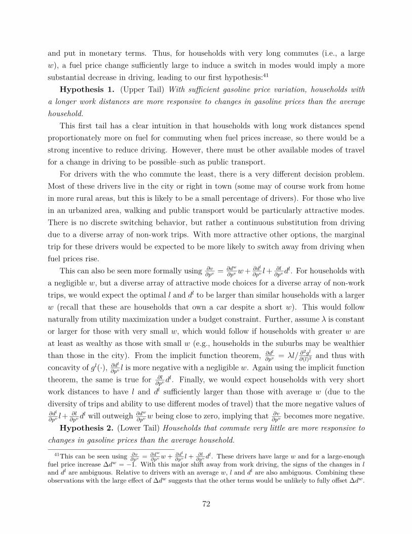
and put in monetary terms. Thus, for households with very long commutes (i.e., a largew), a fuel price change sufficiently large to induce a switch in modes would imply a moresubstantial decrease in driving, leading to our first hypothesis:41

Hypothesis 1. (Upper Tail) With sufficient gasoline price variation, households witha longer work distances are more responsive to changes in gasoline prices than the averagehousehold.

This first tail has a clear intuition in that households with long work distances spendproportionately more on fuel for commuting when fuel prices increase, so there would be astrong incentive to reduce driving. However, there must be other available modes of travelfor a change in driving to be possible–such as public transport.

For drivers with the who commute the least, there is a very different decision problem.Most of these drivers live in the city or right in town (some may of course work from homein more rural areas, but this is likely to be a small percentage of drivers). For those who livein an urbanized area, walking and public transport would be particularly attractive modes.There is no discrete switching behavior, but rather a continuous substitution from drivingdue to a diverse array of non-work trips. With more attractive other options, the marginaltrip for these drivers would be expected to be more likely to switch away from driving whenfuel prices rise.

This can also be seen more formally using ∂v∂pv = ∂dw

∂pv w+ ∂dl

∂pv l+ ∂l∂pv d

l. For households witha negligible w, but a diverse array of attractive mode choices for a diverse array of non-worktrips, we would expect the optimal l and dl to be larger than similar households with a largerw (recall that these are households that own a car despite a short w). This would follownaturally from utility maximization under a budget constraint. Further, assume λ is constantor larger for those with very small w, which would follow if households with greater w areat least as wealthy as those with small w (e.g., households in the suburbs may be wealthierthan those in the city). From the implicit function theorem, ∂dl

∂pv = λl/ ∂2gl

∂(l)2 and thus withconcavity of gl(·), ∂dl

∂pv l is more negative with a negligible w. Again using the implicit functiontheorem, the same is true for ∂l

∂pv dl. Finally, we would expect households with very short

work distances to have l and dl sufficiently larger than those with average w (due to thediversity of trips and ability to use different modes of travel) that the more negative values of∂dl

∂pv l+ ∂l∂pv d

l will outweigh ∂dw

∂pv w being close to zero, implying that ∂v∂pv becomes more negative.

Hypothesis 2. (Lower Tail) Households that commute very little are more responsive tochanges in gasoline prices than the average household.

41This can be seen using ∂v∂pv = ∂dw

∂pv w + ∂dl

∂pv l + ∂l∂pv d

l. These drivers have large w and for a large-enoughfuel price increase ∆dw = −1. With this major shift away from work driving, the signs of the changes in land dl are ambiguous. Relative to drivers with an average w, l and dl are also ambiguous. Combining theseobservations with the large effect of ∆dw suggests that the other terms would be unlikely to fully offset ∆dw.

72

This second hypothesis stems naturally from our model, but is also consistent with pre-vious empirical evidence from the United States indicating that households residing in citiesare some of the most responsive to fuel price changes (Kayser, 2000; Gillingham, 2013, 2014;Gillingham, Jenn, and Azevedo, 2015). This formulation is also more general than householdsthat reside in cities

To be clear, we do not claim that these two hypotheses hold under all conditions (e.g.,without adequate public transport, the upper tail is much less likely). However, they holdunder reasonable assumptions and provide empirically testable implications for the hetero-geneity in the fuel price elasticity of driving in our empirical setting. We also do not claimthat this model provides the only way that two tails might be generated.42

We intentionally developed a simple static model to build intuition for the shorter-rundriving decisions. In a dynamic setting, we would expect to see similar substitution behav-ior, whereby households could “invest” in switching if the discounted savings from doing sooutweigh the switching cost.43 Because the savings equal w times the travel cost differential,households with longer w will switch for smaller changes in the fuel price. Such a mechanismcould also be included in our model by allowing γw to be heterogeneous and increasing inw. For a longer-run analysis, the work distance could be endogenized, but this is outside thescope of our paper, which follows the literature in focusing on the short-run driving decision.

42For example, if one made the assumption that the elasticity increases with fuel demand as a share ofincome and also assumed that this share increases with distance from the city, one could generate the uppertail. Our data suggest that the share may not vary uniformly with distance from the city, so this would bea poor assumption.

43The intuition is similar to the intuition in an (S, s)-model of portfolio choice; for small changes in thefuel prices, most households will stick with their baseline mode choice and avoid paying the switching cost.For larger changes, however, they will be forced to re-optimize.

73