a taxonomy of self-organizing maps for temporal sequence processing
TRANSCRIPT

1
A Taxonomy of Self-organizing Maps
for Temporal Sequence Processing
Gabriela Guimarães a)
Victor Sousa Lobo b) Fernando Moura-Pires c)
a) CENTRIA , Computer Science Department, New University of Lisbon, Portugal
b) Navy Academy, Portugal [email protected]
c) University of Évora, Portugal
[email protected] Abstract
This paper presents a taxonomy for Self-organizing Maps (SOMs) for temporal
sequence processing. Four main application areas for SOMs with temporal processing
have been identified. These are prediction, control, monitoring and data mining. Three
main techniques have been used to model temporal relations in SOMs: 1) pre-
processing or post-processing the data, but keeping the basic SOM algorithm; 2)
modifying the activation and/or learning algorithm to take those temporal
dependencies into account; 3) modifying the network topology, either by introducing
feedback elements, or by using hierarchical SOMs. Each of these techniques is
explained and discussed, and a more detailed taxonomy is proposed. Finally, a list of
some of the existing and relevant papers in this area is presented, and the distinct
approaches of SOMs for temporal sequence processing are classified into the
proposed taxonomy. In order to handle complex domains, several of the adaptation
forms are often combined.
Keywords
Self-organizing Maps, temporal sequences, taxonomy of classifiers, temporal SOMs

2
1 Introduction
The Self-organizing Maps (SOM), proposed by Kohonen [37], also called Kohonen
networks, have been used with a great deal of success in many applications [41].
Since SOMs are neural networks based on unsupervised learning, they have been
widely used for exploratory tasks [16],[34]. The main aim here is to discover patterns
in high dimensional data and find novel patterns that might be hidden in the data. This
often assumes an adequate visualization of the network structures, such as component
maps [64], U-matrices [68], or a hierarchical and colored visualization of the SOM
[24],[55],[76]. However, the basic SOM is designed to map patterns, or feature
vectors, from an input space (usually with high dimensionality) into an output space
(usually with a low dimensionality), and does not take time into account. Many
different approaches have been taken to adapt the basic SOM algorithm for time
sequence processing, each with it's particular advantages and drawbacks, and some
are reviewed in [12],[23],[41]. We shall call these adaptations of the original SOM
temporal SOMs. In this paper, we will identify the main ideas that have been
proposed, and establish a taxonomy for temporal SOMs. We will also provide
examples of applications of those techniques and discuss their relative strengths and
interdependencies. We will not focus on the details of their implementations, for
although they may be crucial to the success of certain applications, they do not bring
relevant insight on how to take time into consideration when using SOMs.
Temporal SOMs have been used in a wide variety of applications, usually for one of
the following purposes: prediction [44],[70],[74], control [59],[61], monitoring [28],
and data mining [16],[21],[22].
The main rationale for using SOM instead of other temporal algorithms resides on its
inherent ability to provide several simple local models for the sequence, one model

3
for each of the maps units. Moreover, those different models are topologically ordered
in such a way that similar models are grouped together. A discussion on the more
basic reasons for using SOM-based methods for temporal sequence processing can be
found for example in [20],[43].
At a first glance, there are three main “families” of temporal SOMs: those that use the
basic SOM algorithm without considering time explicitly (using time only during pre-
or post-processing); those that modify the learning rule (and/or the classification rule)
to reflect temporal dependencies; and finally those that modify the topology of the
basic SOM, either by introducing feedback, or by introducing a hierarchical structure.
Each of these basic ideas can then be implemented using different techniques, giving
rise to a number of different SOMs that we shall group according to Fig. 1.
In section 2 we describe the approaches based on unmodified SOMs where the pre-
processing and post-processing techniques for handling temporal sequences are
presented. Pre-processing techniques are often based on time-delay embedding or
some type of domain transformations. Post-processing techniques include mainly
visualizations of the network results, such as paths, i.e. trajectories, that are displayed
on the map. Section 3 discusses adaptations of the learning algorithm that are mainly
used for control and prediction tasks, where the fundamental techniques are
Hypermaps and the maps proposed by Kangas [30] – here referred as Kangas Maps.
In section 4, modifications of the network topology for temporal sequence processing,
such as feedback and hierarchical SOMs, are discussed. Some conclusions and a
classification of the approaches into a scheme are presented in section 5.
We cannot at this time present benchmark comparisons between the different
approaches. When proposing various approaches, different authors have used many
different datasets, and have used different criteria when accessing performance. This

4
makes direct comparisons between approaches proposed in different papers
impossible. Even if benchmark comparisons where available, the best approach for
any given problem would not always be obvious, given the high dependence of
performance on the particular characteristics of the data and on the criteria used to
assess that performance.
2 Temporal Sequence Processing with unmodified SOMs
In this section we discuss two distinct approaches of SOMs for handling temporal
sequences that do not afford a modification of the original algorithm or network
topology. One of the approaches concerns the pre-processing of a temporal sequence
before presenting it to the neural network, and therefore embedding time into the
pattern vector. The other approach is related to some kind of post-processing of the
network outputs, resulting in a time-related visualization (or processing) of the data on
the map with trajectories. In the following subsections both approaches, and several
related applications will be presented.
2.1 SOMs with Embedded Time
Basic Idea
The common denominator of embedded time approaches is that some sort of pre-
processing is performed on the time series before it is presented to the SOM. Thus, the
SOM receives an input pattern that is treated in the standard manner, as if time was
not an issue.
Variants
There are several ways to “hide“ time in the pattern vector, which may require more
or less pre-processing and knowledge of the underlying process. A simple tapped

5
delay will provide the easiest way of generating a pattern vector. On the other hand, a
complex feature extraction algorithm may be used to generate that vector.
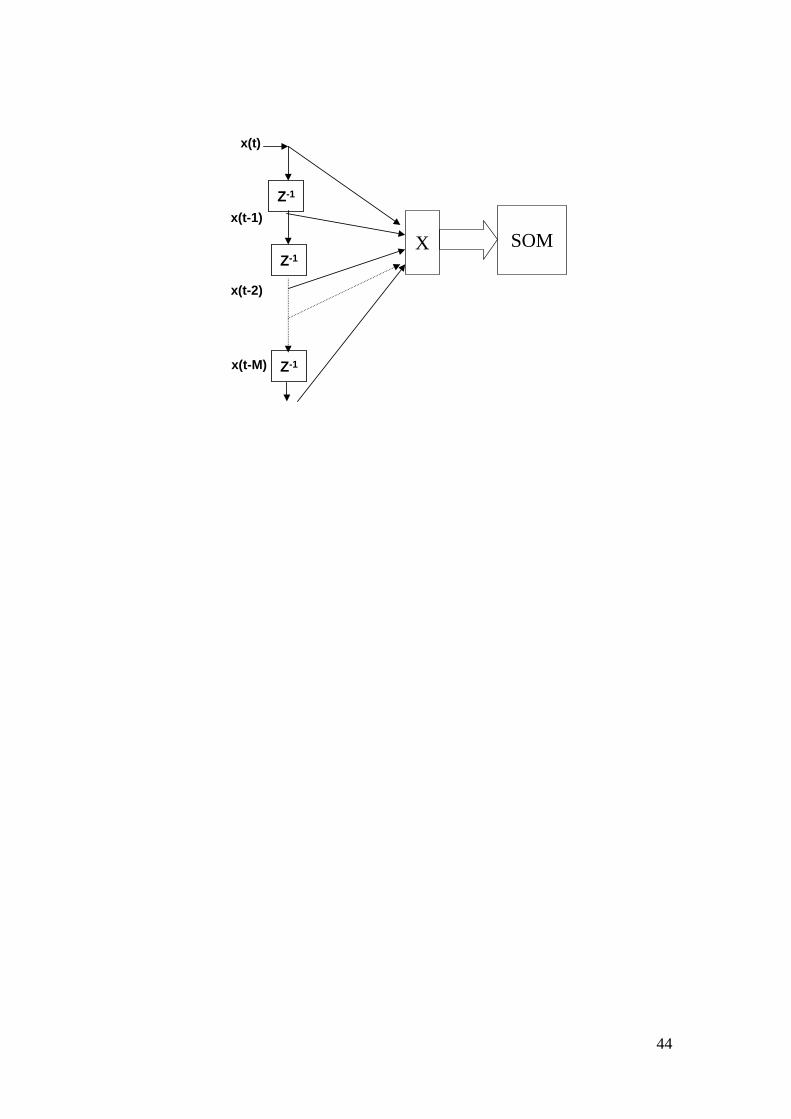
Variant 1 - Tapped delay SOMs
The simplest pre-processing step used when applying SOMs to temporal sequences, is
to use a tapped-delay of the input as pattern vector [11]. The SOM is thus presented
with a pattern that is a vector of time-shifted samples of the temporal sequence, i.e. it
receives a "chunk" of the temporal sequence instead of just it's last value, as is shown
in Fig. 2. This approach was followed by some of the early applications of SOM [29],
and is still quite popular when feature extraction techniques (e.g. Fourier transforms,
envelopes, etc) are not necessary [57]. Some authors also name it Time-Delay SOM
[32], since the approach is basically the same as the popular backpropagation-based
Time-Delay Neural Networks (TDNN) proposed by [47] and [80].
This is a very intuitive and simple way of introducing time into the SOM, and has
proved to give good results in many situations. It does however have a few known
drawbacks.
On one hand, the length of the tapped delay (the number of samples used) has to be
decided in advance, and the ideal length may be quite difficult do determine. If too
few time points are used, the dynamics of the sequence will not be captured. If too
many are used, apart from having an unnecessarily complex system, it may be
impossible to isolate smaller length patterns. This problem also arises in other
approaches, as discussed in [15],[58].
On the other hand, since the basic SOM is not sensitive to the order in which the
different dimensions of the input pattern are presented, it will not take into account the
statistical dependency between successive time points. It is interesting to note that

6
using this approach, the order of the successive time points in the final pattern vector
is irrelevant (as long as that order is kept constant).
Variant 2 - Time-related transformations
In many applications, there are features of temporal sequences that are better
perceived in domains other then time. The general structure of this approach can be
seen in Fig. 3. The most commonly used domain is frequency, and the most used
technique is to perform a short-time Fourier transform on the data [39]. Many other
transformations have been used, such as cepstral features [30], wavelet transforms
[46],[53],[56], and time-frequency transformations [2],[27]. In fact, many of the
practical applications of temporal SOMs use some sort of time-related transformation
as a first step in the pre-processing of the data, even if time is taken into account at a
later stage. The success of these techniques is strongly dependent on the
characteristics of the problem at hand, and has little to do with the inherent properties
of the SOM.
Discussion
These types of approaches, where only pre-processing of the data is used to deal with
time, have the advantage that they preserve all the well-known characteristics of the
SOM algorithm. Moreover, from a engineering point of view, they allow a simple
integration of standard SOM software packages with the desired pre-processing
software. These techniques of embedding time into the pre-processing are quite
universal, and can be used to adapt almost any pattern-processing algorithm to
temporal sequence processing.

7
Examples
One of the early papers on SOMs Kohonen [38] uses this technique. In this paper,
what would later be known as the “phonetic typewriter”, was prototyped.
In [48], for example, where the objective was to detect dysphonia, the short time
power spectra of each 9.83s chunk of signal (spoken Finnish) was calculated using
256 point FFT. The logarithms of that power spectra where then calculated, and
smoothed with a low pass filter. Finally 15 of the resulting bins were selected as
features, and fed into a basic SOM.
In [51], the objective was to identify different classes of ships, using the sound they
make in the ocean. The sound was recorded using commercial sound cards and
military sonar equipment. Originally a 22 KHz-sampling rate was used, but since the
equipment had high quality filters at 2 KHz, the signal was then re-sampled to a 5.5 K
samples/s rate. After that, segments of signal with 4096 data points were extracted,
with a 50% overlap between consecutive samples (so as to achieve a good
compromise between bias and variance), and a Hamming window was applied to it.
An FFT was performed on each segment to calculate it’s power spectrum, and the
2048 bins of positive frequencies where used as features. So as to increase the signal
to noise ratio, the actual features used were the averages of 4 consecutive power
spectra. The patterns thus obtained where fed to a SOM, and the results, in the form of
a blinking cursor over a labeled map, where displayed to the operator. The system was
successful on a number of trials involving different training sets, with up to 30
different types of ships.

8
2.2 Trajectory-based SOMs
Basic idea
Apart from pre-processing the inputs, we can also consider using a basic SOM,
without considering time during the learning process, and then post-process the results
obtained during the classification phase. The most popular of these methods are what
we call Trajectory-based SOMs. These consider temporal relations among succeeding
best-match units. This means that at each time point t=1,...,N, the best-match ut,,t ∈
{1,…,N}, representing the input vector is searched and recorded on the map. Then, a
representation of time-related input vectors on the map is made by joining k
succeeding best-matches ui,…,ui+k-1, i∈{1,...,N-k} connected forming a path, as can be
seen in Fig. 4. These paths are often named trajectories (hence the name of this
technique).
Discussion
Trajectory-based SOMs, as opposed to the approaches presented before, constitute a
genuinely new way of dealing with time. It is impossible to use “trajectories” in
methods such as feed-forward neural networks or classical filters, because the
topological information provided by SOMs is missing. In fact, these trajectory-based
methods are successful because they explore this topological ordering, extrapolating it
into the time domain.
It is interesting to see that even though training is done ignoring any sort of time
dependency (and thus training data may be collected in any manner), temporal
information can be recovered during the classification phase, revealing structures of
the underlying process.

9
Another interesting feature of these methods is that information can be obtained from
the direction of the path and not it’s exact location. Thus, for example, if we have a
map trained with faulty instances of a given process, we do not need to wait until that
region of operation is reached, i.e., if the winning unit moves towards that region, we
can predict something is wrong before it actually occurs [67],[69].
When processing the trajectories, it may also be important to determine the amount of
successive best matches to consider, i.e., the temporal length of the trajectory. This
problem is similar to the problem of determining the number of time points in a
tapped delay, mentioned before.
Trajectories are often combined with other visualization techniques for the graphical
representation of the weights of a learned SOM. These are, for instance, component
maps where one of the components of the weights is projected onto a third dimension,
as well as U-Matrices [68], where the distances between neighboring units calculated
in the original space, i.e. the weights, are projected onto a third dimension. Often
these additional visualization techniques lead to an enhanced interpretation of the
trajectory.
Other interesting visualization techniques for SOMs have also been proposed, such as
the agglomerative clustering where the SOM neighborhood relation can be used to
construct a dendrogram on the map [55],[76], and a hierarchical clustering of the units
on the map with a simple contraction model [24]. Although these approaches have not
yet been used in the context of temporal sequence processing, they would enable a
richer perception of the significance of the trajectory, allowing varying levels of detail
in the analysis of the inputs.
For most applications trajectories have been directly displayed on a map without a
visualization of the network weights [39],[49]. In those cases a direct interpretation of

10
the trajectory is possible if a prior classification of the signal exists, as for example, in
different phoneme types in speech recognition [39] or distinct sleep stages in EEG
signals [33]. However, if the SOM is used as a feature extractor, the trajectory itself,
regardless of any labeling, can be used as a temporal feature of the input, and fed to a
higher level system [66]. For example, if we train an unlabeled SOM with phonemes,
a given word will have a distinct path that would distinguish it from other words. If
we are using the SOM as a visualization tool and no prior information on the classes
is known, a combination of trajectories with other visualization techniques for SOMs
mentioned earlier (component maps, U-matrices, and hierarchical clustering
visualizations), can be very useful.
Component maps enable to track the trajectory along a single component. This can be
advantageous, if we are interested in evaluating the contribution of each of the
components to the system‘s state changes. Notwithstanding, if a large number of
variables have to be considered, this approach can originate some confusion and
unclearness to the observer. In order to overcome these disadvantages, we will have to
observe the development of a complex system or process on a single map using, for
instance, U-matrices.
The main advantage in visualizing trajectories on U-matrices lies in the identification
of state transitions. These transitions are clearly seen on a U-matrix, because when
one such transition occurs, the trajectory of the best-match unit has to overcome a
“wall”. This means that in the original space a large distance has to be traveled, if a
trajectory jumps over a wall, even if the distances on the map itself are small, i.e. they
are neighboring units. This type of interpretations is not possible if the trajectories are
observed only on the SOM itself.

11
Examples
The visualization of trajectories on the map itself was first applied to speech
recognition [39]. Here a decomposition of a continuous speech signal is performed in
order to recognize phonetic units. Before presenting the data to the network, a
transformation into the frequency domain is made. A map, named here as phonotopic
map, was generated with the input vectors representing short-time spectra of speech
waveform computed every 9.83 milliseconds. One of the most striking results was
that various units of the network became sensitized to spectra of different phonemes
based only on the spectral samples of the input. However, in this approach samples
only correspond to quasi-phonemes. Now, one of the problems lies in the
segmentation of quasi-phonemes into phonemes. For this purpose, the degree of
stability of the waveform, heuristic methods, and trajectories over a labeled map were
calculated. Convergence points of the speech waveform then may correspond to
certain stationary phonemes. The main advantage of phonotopic maps is that they can
be used for speech training or therapy, since people can obtain immediate feedback
from their speech.
This approach was also widely applied at the early 90‘s to several medical
applications, such as the identification of co-articulation variation and voice disorder
[71], the detection of fricative-vowel coarticulation [49], the detection of Dysphonia
[48], the acoustic recognition of “/s/” misarticulation enabling a distinction between
normal, acceptable and unacceptable articulations [54], the recognition of topographic
patterns in EEG spectra from 16 subjects having different sleep/awake stages [28],
and the monitoring of EEG signals enabling the identification of six typical EEG
phenomena, such as well organized alpha frequencies, eye movement artifacts and
muscle activity [33]. All these approaches have in common that a pre-classification of

12
the original signal was already made. In applications for speech processing such a pre-
classification is always possible. Within another approach for speech recognition
trajectory-based SOMs have been used at different hierarchical levels (discussed later
in this paper), where each layer operates on a different time scale and deals with
higher units of speech, such as phonemes, syllables, and word parts [5]. This means
that the basic structure of all layers is similar, only the meaning of the input and the
time scale are different. This approach was used for the recognition of normally
spoken command sentences for robot controlling, whereat the system had to deal with
extra words and other insertions not part of a robot command. So, syntax and
semantic modeling also played here an important role. Trajectories have only been
used at the first level. They consist of stationary parts representing vowels that remain
in a close neighborhood and transitions paths with jumps to different and more distant
parts of the map. In order to distinguish between stationary and transition parts, a
critical jump distance separating short and long distances, as well as a minimum
segment length was defined.
Trajectory-based SOMs have also been proposed to model low dimensional non-
linear processes, such as non-linear time series obtained from a Markey-Glass system
[57]. They followed three steps: the reconstruction of the state space from the input
signal; the embedding of the state space in the neural field; and the estimation of
locally linear predictors. Trajectories are then used to obtain a temporal representation
of all 400 consecutive input samples.
Within another application firing activities in monkey’s motor cortex have been
measured and presented to a SOM in order to predict the trajectory of the arm
movement, especially while the monkey was tracing spirals and doing center-out
movements [50]. From the map, three circle-shaped patterns representing the spiral

13
trajectory have been identified through paths on the map. The results showed that the
monkey’s arm movement directions are clearly encoded in firing patterns of the motor
cortex.
In [35], for instance, component maps are used for process state monitoring where
values for one parameter are visualized as gray values on a map. The lighter the unit
on the map, the higher the parameter value is. Their aim was to classify the system
states and detect faulty states for devices based on several device state parameters,
such as temperature. Faults in the system could be detected with trajectories, if a
transition to a forbidden area on the map marked with a very dark color occurred. This
approach was also applied to process control in chemistry for monitoring a distillation
process [67].
Visualization of trajectories on U-matrices have been used for monitoring chemical
processes [69], and have been applied to complex processes, such as the dynamic
behavior of a computer systems with regard to utilization rates and traffic volume
[63], to industrial processes, such as a continuous pulp digester, steel production and
pulp and paper mills [1], and to different subjects with distinct sleep apnea diseases
[22]. In order to enhance exploratory tasks with SOM-based data visualization
techniques, quantization error plots can be used using bars or circles on both,
component maps or U-matrices [75].
3 Modification of the Activation/Learning Rule
Another possibility for processing temporal data with SOMs lies in the adaptation of
the original Kohonen activation and/or learning rule. Here we distinguish between
two distinct approaches. In the first, the input vector is decomposed into two distinct
parts, a past or context vector and a future or pattern vector. Both parts are handled in
different ways when choosing the best match and when applying the learning rule.

14
This approach, named Hypermap, was first introduced by Kohonen [40]. The second
approach, what we will call Kangas map, searches for the best match in a
neighborhood of the last best match.
3.1 The Hypermap Architecture
Basic ideas
In this architecture the input vector is decomposed into two distinct parts, a “past” or
“context” vector and a “future” or “pattern” vector. The basic idea, now, lies in
treating both parts in different ways. The most common way is to use the context part
to select the best match or “best-match region”, and then adapting the weights using
both parts, separately or together. However many variants exist, and will be discussed
later.
For time series a Hypermap means that the future (prediction) is learned in the context
of it’s past. During the classification phase the prediction is made using only the
“past” vector for the best-match search. Thus, the SOM is used as an associative
memory, and the “future” part of the vector is then retrieved from the weights of the
map associated with the best match.
Discussion
Originally the Kohonen algorithm is an unsupervised learning algorithm that can be
used for exploratory tasks. Approaches, however, that use some kind of Hypermap
architecture, perform a profound change in the interpretation of the original Kohonen
algorithm towards a supervised learning algorithm, since an output vector (the future
or pattern vector) is added to the input (the past or context vector). This makes sense
in applications that require an extrapolation of the data into the future as, for example,
in time series prediction [70], or in robot control [60].

15
Examples
This approach was first introduced by Kohonen [40] and named Hypermap
architecture. It was applied to the recognition of phonemes in the context of cepstral
features. Each phoneme is then formed as a concatenation of three parts of adjacent
cepstral feature vectors. The idea was to recognize a pattern that occurs in the context
of other patterns, where x(n) = [xpatt(n), xcont(n)]. A two-phase recognition algorithm
for the best-match search was proposed. In the first phase, we start by selecting a
“context domain”. This is done by searching for the “good”-matches within the
context, i.e. all units that are within a given distance of the context vector xcont(n). In
the second phase, the best match is searched within the selected context domain, using
only the pattern xpatt(n). During learning we also have two phases. In the first phase, a
context SOM is trained using only the context xcont(n) and the basic SOM algorithm.
After this SOM is trained, its weights are frozen (i.e. made constants). Next, we
perform a learning of the pattern weights of the Hypermap. This is done using the
above described algorithm for the best-match search, but performing the adaptation
only on the unit weights that are related to the pattern vector xpatt(n). Furthermore, for
this particular application, an extra-supervised learning step was used to associate the
units with phonemes.
This architecture was generalized in [6] to perform hierarchical relationships having
n-1 levels defining the context for the classification of EEG signals from acoustical
and optically evoked potentials. This type of model was also studied for phoneme
recognition using the LASSO model [52], for simulating a sensory-motor task [59], as
well as for robot control [60],[61],[81],[83]. In this latter application, the output is the
target position of the robot arm (for instance, given by the angles), while the input is

16
given as a four-dimensional vector describing the spatial position of the robot arm
obtained by the images of two cameras.
Hypermaps have also been used for prediction tasks, for instance, using SOMs for
local models in the prediction of chaotic time series [45]. The time series is embedded
in a state space using delay coordinates x(n) = [x(n), x(n-1),…, x(n-(N-1))], where N is
the order of the embedding. The embedded vector is then used to predict the next
value of the series x(n+1). The following vector y(n) = [x(n), x(n+1)] is presented to
the map during the learning phase. However, when searching for the best match, the
target value is left out. This means that only the first part (past) of the whole vector is
used for the determination of the best match. During learning, the unit weights are
adapted using the whole input vector, and the standard Kohonen algorithm. Now,
during the classification phase, only the first part of the vector is used for the best-
match search, and indeed it is the only part available, since we are trying to predict the
future. Thus this future part is obtained through an associative mapping with the past.
In [70] a two step implementation of this approach was used for the prediction of
hailstorm. First, it was used to identify distinct types of hailstorm developments. After
the classification part, prediction was made using the completed vector.
3.2 Kangas Map
Basic ideas
Instead of considering explicitly the context as part of the pattern, as is done in the
Hypermap, we may consider that the context is given by the previous best-match. In
this case we can use only the neighboring units of the previous best match when
choosing the next one. This idea was proposed by Kangas [30], and so we named this
approach Kangas Maps. In this approach, the learning rule is exactly the same as in

17
the basic SOM. The selection of the best-match is also the same, except for the fact
that instead of considering all units for the next iteration step, only those in the
neighborhood of the last best-match are considered, as mentioned before (see Fig. 5).
Discussion
This type of map has several interesting features, and can in certain cases have a
behavior similar to SOMs with feedback, e.g. SOMTAD [20], discussed later in this
paper.
From a engineering point of view, it can be considerably faster then a basic SOM
when dealing with large maps, since we only need to compute the distances to some
of the units. It also requires very little change in the basic SOM algorithm, and keeps
its most important properties. The area where the next best-matches are searched for
acts as a “focus region”, where the changes in the input are tracked. In a Kangas map,
we may have various distinct areas with almost the same information (relating to the
same type of input signal), but with different neighboring areas. Thus, the activation
of the units will depend on the past history, i.e. on how the signal reached that region
of the map. Thus, this approach uses the core concepts of neighborhood and
topological ordering of SOMs, to code temporal dependency.
In the original paper [30] some variants of the basic idea are proposed, though not
explored in depth. One of them allows for multiple best matches, and thus multiple
tracking of characteristics of the input signal.
A similar approach, that also uses feedback (discussed later in this paper) was
proposed in [9], and named Spatio-Temporal Feature Map (STFM). In a STFM, the
units that are used when searching for a best-match are selected according to a rule
that includes more than just the neighborhood (in the output space) to the last best-
match. Two core concepts are used in this selection: a so-called spatial grating

18
function that basically defines a spatial area of influence of each unit; and a gating
function, that is a time-dependant function of past activations, and determines the
output of the units. Using these two concepts, a so-called competition set of units is
selected, where the winner will be searched. Finally, in the above-mentioned papers,
the trajectory of the best match is also used, and named the “spatio-temporal
signature” of the temporal sequence.
Many other rules may be used to select the candidate best matches.
Instead of using past activations to select candidates for best matches, we can also use
those past activations to exclude certain candidates. The Sequential Activation
Retention and Decay NETwork (SARDNET), proposed in [25] does just this. In this
approach (which also uses feedback), the best match is excluded from subsequent
searches. Thus, a sequence of length l will select l different best matches, or a l-length
trajectory. As discussed in [25] this will force the map to be more detailed in the areas
where each of the sequences occur, thus representing small variations of those
sequences with greater detail. A decay factor is also introduced to make the selection
of the best-match depend on past activations, but we will not discuss it’s influence
here. This hybrid approach was used successfully to learn arbitrary sequences of
binary and real number, as well as phonetic representations of English words.
Kangas Map based approaches have been used for speech recognition tasks [30],[32],
texture identification, and 3-D object identification [9],[10].
4 Modification of the Network Topology
The third possibility in handling temporal data lies in modifying the network
topology, introducing either feedback connections into the network or several
hierarchical layers, each with one or more SOMs. Feedback SOMs are intimately
related to digital filters and ARMA models, which are a more traditional way of

19
dealing with temporal sequences. The latter approach is mainly used when a
segmentation of complex and structured problems is needed in application domains,
such as image recognition, speech recognition, time series analysis, process control,
and protein sequence determination.
4.1 SOMs with Feedback
Basic Idea
One of the classical methods to deal with temporal sequences, which have been used
with great success in control theory, is to feed some sort of output back into the
inputs. This is usually done with an internal memory that stores past outputs, and uses
them when generating the next outputs. One of the advantages of these methods is that
they do not require the user to specify the length of the time series that must be kept in
memory, as happens with the tapped-delay approaches.
Variants
There are a few different values that can be used for feedback, and a few different
ways to introduce these values back into the system. Thus a large number of
approaches have been proposed and tested in different environments.
Variant 1 - Temporal Kohonen Maps (TKM)
Historically, the first well-documented proposal for feedback SOMs appeared in 1993
[13], named as “Temporal Kohonen Map” (TKM), and is very similar to the model
used in [30]. The main idea behind this approach lies in keeping the output values of
each unit and using them in the computation of the next output value of that unit. This
is done by introducing a leaky integrator in the output of each SOM unit. In a TKM
the final output of each unit is defined as
Vi(n) = α Vi(n-1) - ½ || x(n)-wi(n) ||2 (1)

20
where
Vi(n) is the scalar output of unit i, at time n
Vi(n-1) is the scalar output of unit i, at time n-1
x(n) is the input pattern presented at time n
wi(n) is the SOM unit i, at time n
α is a time constant called decay factor, or memory factor, restricted to
0 < α < 1.
The best-matching unit is considered to that which has a higher Vi(n) (which is always
negative). The learning rule used is that of the basic SOM. When α =0, the units have
no memory, and we fall into the standard SOM algorithm. It must be noted that this
output transfer function resembles the behavior of biological neurons, which do have
memory, and weigh new inputs with past states.
In essence, for the sake of comparing this approach with others, the activation
function (to be minimized) is
Vi(n) = α Vi(n-1) + (1-α ) || x(n)-wi(n) || (2)
This formulation of the TKM is shown in Fig. 6.
Variant 2 - Recurrent SOM (RSOM)
The TKM keeps only the magnitude of the output of the units, and keeps no
information about each of the isolated components, and thus no information about the
“direction” of the error vector. To overcome this limitation, the Recurrent SOM
(RSOM) was proposed [14],[72], where the leaky integrators are moved from the
output to the input of the magnitude computation. As a consequence, the system
memorizes not only the magnitude, but also the direction of the error.
The activation function for each unit will now be
Vi(n) = || yi(n) || , (3)

21
where yi(n) is the error vector given by
yi(n) = (1-α) yi(n-1) + α( x(n)-wi(n) ) (4)
This formulation of the Recurrent SOM is shown in Fig. 7.
Recursive SOM
The TKM uses, for the computation of the activity of each unit, only the previous
output of that unit. The RSOM also uses only local feedback. Another alternative is to
feedback the outputs of all the units of the map to each of them. This alternative was
first proposed in [79], later in [3], and was analyzed in detail in [77],[78], and with
slight modifications in [62]. The latter authors first named this approach Contextual
Self-Organizing Map (CSOM), and later Recursive SOM. In this paper we use the
name Recursive SOM to clearly differentiate it from the Hypermap architecture that
also uses the term “context”. The dimensionality of each unit is increased
significantly. Besides the standard weight vector wiinput each unit i will also have a
weight vector wioutput, which is to be compared with actual outputs in the previous
instant. The activation function defined by [78] is
Vi(n) = exp( -α || x(n)-wiinput(n) || 2 – β || V(n-1)-wi
output(n) || 2), (5)
where α and β are constant coefficients that reflect the importance of past inputs.
The formulation of the Recursive SOM is shown in Fig. 8.
SOM with Temporal Activity Diffusion (SOMTAD)
Another approach, similar to recursive SOM, was proposed and analyzed in
[17],[18],[19],[20],[42] and, in the latter paper, named SOM with Temporal Activity
Diffusion (SOMTAD). In a SOMTAD, instead of feeding back all past outputs (and
learning their respective weights), only the activations of neighboring units are fed
back. This leads to a sort of shock wave that is generated in the best match unit, and

22
propagates throughout output space of the map. Adapting the proposed algorithm to
the formalism we have been using, we will have
Vi(n) = (1-α) Vi(n-1) + α || x(n)-wi(n) || (6)
just as in a KTM, but each unit i will also have an enhancement E given by
Ei = f( Vneighbour(t-1)) (7)
where f(.) is some function, that couples the enhancement of one unit with the activity
of it’s neighbor.
The best match is then
best-match(t) = arg min( || x(n)-wi(n) || + β Ei(t) ) (8)
where β is called the spatio-temporal parameter, and controls the importance of past
neighboring activations. The structure of each unit of a SOMTAD is shown in Fig. 9.
It must be noted that when β tends to 0, the SOMTAD becomes a standard SOM. As
it increases, the behavior will be similar to a Kangas map, since the best match will
tend to be in the vicinity of the last best-match, and as β tends to +∞, the model
degenerates into an avalanche network.
Discussion
None of the above proposals is universally better then any other, so one can always
find an example of an application where a given approach outperforms the others.
There are, however, some well-known characteristics that can help us choose a good
approach for a given problem. A good theoretical comparison of the Temporal
Kohonen Map (TKM) and the Recurrent SOM (RSOM), can be found in [73], where
the authors show that TKM lacks RSOM’s consistent update rule. Thus, while a
RSOM will converge to optimum weights for its units, following a gradient descent
algorithm, the TKM will not, hence in some way it will be unreliable. In a series of

23
experiments, the authors show that generally a RSOM will provide a more efficient
mapping of the input space signals then a TKM, which tends to concentrate it’s units
in certain regions of that space. On the other hand in [78] it is shown that for a
classical benchmark problem, the Mackey-Glass chaotic time series, the Recursive
SOM will provide a far better mapping then the Recurrent SOM. This will generally
be the case when a global perspective of the signal space is necessary, which means
that in those cases, when a global perspective of the past inputs is necessary, a strictly
local approach, such as TKM and RSOM, can not give good results. However, it must
be noted that the complexity of the system is also considerably increased when we use
a Recursive SOM.
Examples
Recurrent SOMs have probably been the most used model. They have been
successfully applied to the Mackey-Glass Chaotic Series, infrared laser activity, and
electricity consumption [43], as well as clustering of epileptic activity based on EEG
[45]. As described earlier, the Recursive SOM was also used to study the Mackey-
Glass series, and has outperformed the RSOM. It was also used, with slight
modifications, in [62]. To our knowledge, the SOMTAD model has only been applied
by it’s authors to digit recognition, and to small illustrative problems in
[17],[18],[19],[20].
4.2 Hierarchical SOMs
Basic idea
Hierarchical SOMs are often used in application fields where a structured
decomposition into smaller and layered problems is convenient. Here, one or more
than one SOMs are located at each layer, usually operating at different time scales

24
(see Fig. 10). Hierarchical SOMs in temporal sequence processing have been
successfully applied to speech recognition [26],[36], electricity consumption [8],
vibration monitoring [27], motion planning [3]and temporal data mining in medical
applications [21].
Discussion
The main difference between hierarchical SOMs lies in the type of codification of the
results of one level SOMs to the next upper level. They also differ in the number of
levels used, which strongly depends on the type of application. Finally, they differ in
the number of SOMs at each level, and the interconnections between the levels.
The rationale for using hierarchical SOMs is that of “divide and conquer”. By
focusing independently on different inputs we do lose information, but we gain
manageability. We can thus use a relatively low complexity model, such as a SOM to
handle each of the small groups of inputs, and then fuse this partial information to
extract higher-level results. Good results can thus be obtained with hierarchical SOMs
in complex problems that cannot be modeled by a single SOM [21].
There are mainly three different ways to calculate the input vector for the next level
SOM. First, the weights of the lower-level SOM are used as input without any further
processing, either taking into account the information of the previous known classes
[36] or without considering any information on the classes [82]. In this case, the first
level SOM is simply being used for vector quantization. Second, a transformation of
the network results is possible, for instance: 1) calculating the distances between the
units [7]; 2) concatenating subsequent vectors into a single vector, thus representing
the history of state transitions [63]; or 3) taking into account the information about
clusters formed at this level, and adjusting the weights towards the cluster center [21].

25
The third possibility lies in interposing other algorithms or methods, such as segment
classifiers [5].
Examples
This approach was first introduced in speech recognition, where each layer deals with
higher units of speech, such as phonemes, syllables, and word parts [5],[36]. For
instance, in [5] at each layer a SOM operating at different time scales is used, which is
connected to a segmentation unit for the segmentation of the input and to
segmentation classifiers. Each of the classifiers was trained to recognize a special
class of segments, thus producing an output vector for each segment. These output
vectors, i.e. the activities of the classifiers, form the input for the next level, which
thus operates on a larger time scale. Each segment classifier m produces an output
activity am = Σi ci·wim, ci denoting the activity of the SOM unit i and wim the synaptic
strength from SOM unit i to classifier m. These connections may be inhibitory
(wim<0), but always fulfill Σiw2im=1.
In [26] a speaker recognition system based on the auditory cortex model is proposed.
Since an auditory cortex can be generally considered as a layered upward structure
with complex connections, three hierarchical levels of SOMs with local connections
have been introduced. The output of the first map contains leaky integrators and is
calculated as follows:
yi(n) = α ⋅ (k / (1 + ||wi(n)-x(n)||)) + (1 - α)⋅ yi(n – 1) , 0 < α < 1 (9)
For the sake of comparison with other approaches, this equation can be transformed
into the following that should be minimized:
yi(n) = (1 - α)⋅ yi(n – 1) + α ||wi(n)-x(n)|| (10)

26
The units of the second and the third layer have input connections from the units of
the immediately lower level. Additional connections exist from the first to the third
level.
Kemke and Wichert [36] also used hierarchical SOMs at different time scales, as
mentioned before. The codification of the input at the next layer is based, however, on
a pre-classification of the signal. A class is associated with each unit on the map. In
order to calculate the output for a given input vector, the mean of the weights of all
units belonging to the class is calculated, and used as input to the map of the next
higher-level map.
Hierarchical SOMs have also been applied to monitoring and modeling the dynamic
behavior of complex industrial processes, such as the dynamic behavior of a computer
system [63]. The main problem in process analysis is to find characteristic states or
clusters of states that determine the general behavior of the system. In this approach, a
hierarchical SOM with two levels was constructed containing a “state map” used to
track the operating point of the process with trajectories, and a “dynamics map” used
to predict the next state on the state map. Each unit on the dynamics map then
represents a "path" leading into the corresponding state. The training set of the state
map for the dynamics map is formed by concatenating subsequent vectors into a
single vector, representing the history of state transitions. In prediction, the state map
vector having the best matching trajectory in its dynamics map is then the predicted
state.
An application of hierarchical SOMs in medicine, namely in sleep apnea research, is
given in [21]. Here, SOMs are used at different hierarchical levels, in order to handle
the complexity given by the large number of signal channels. At the lowest level,
primitive patterns in multivariate time series are discovered for distinct time series
27
selections, while more complex patterns are identified at the next higher-level SOM.
This approach considers the patterns obtained by the low-level maps, using the
information provided by the U-matrix to identify the clusters. Thus, based on this
information, a cluster center is calculated, and in order to calculate the input to the
next-higher level map, all weights are approximated towards it’s cluster center ck
according to the following adaptation rule:
wi,new = wi + α ||wi - ck||, if ck > wi
and
wi,new = wi - α ||wi - ck||, if ck ≤ wi. (11)
A two-level hierarchical SOM has also been applied to short-term load forecasting
[8], and to music data, the Bach’s fugue [7]. In this approach the input to the second
layer SOM is determined by the distance between the best-match ui(n) and all the
other k units of the map uj(n), j≠i, leading to a k-dimensional input vector.
A hierarchical approach to parameterized SOMs (PSOMs) was proposed by Walter
and Ritter [82], in order to cope with only a very few number of examples. This
approach was applied to rapid visuo-motor coordination. One possible solution is to
split the learning into two stages, both on distinct PSOMs: 1) a first level PSOM,
considered as an investment stage for a pre-structuring of system, which may process
a large number of examples; and 2) a second level PSOM, named as Meta-PSOM,
that now is a specialized system with fast learning, and only needing a few examples
as input. The weights of the first level are then used as input to the second level Meta-
PSOM.

28
5 Conclusions
In this paper, a taxonomy for classifying distinct approaches with Self-organizing
Maps (SOMs) for temporal sequence processing was proposed. The focus was put on
the identification of the core concepts involved serving as a framework both for those
studying temporal SOMs for the first time, and for those developing new algorithms
in this area. Naturally, our taxonomy is not complete and exhaustive, in the sense that
more specific and detailed approaches do exist or can be developed in the future.
Also, due to the large number of papers involving SOMs for temporal sequence
processing, and due to the somewhat fuzzy borders of what are or are not temporal
SOMs, many papers that could be considered relevant are not referenced.
We identified three main approaches for temporal sequence processing with SOMs.
These are: 1) methods requiring no modification of the basic SOM algorithm, such as
embedded time and trajectory-based approaches; 2) methods that adapt the activation
and/or learning algorithm, such as Hypermaps or Kangas Maps; and 3) methods that
modify the network structure, introducing feedback connections, or hierarchical
levels. The use of each of these approaches, which are not mutually exclusive,
depends highly on the application, and none is universally better than any other. The
best results are usually obtained by using a carefully tailored combination of these
methods. Table 1 provides a classification of some existing and relevant approaches in
the proposed taxonomy.

29
References
[1] E. Alhoniemi, J. Hollmen, O. Simula and J. Vesanto, Process Monitoring and
Modeling using the Self-Organizing Map, Integrated Computer-Aided
Engineering 6(1) (1999), 3-14.
[2] L. Atlas, L. Owsley, J. McLaughlin and G. Bernard, Automatic feature-finding
for time-frequency distributions, in: Proceedings of the IEEE-SP International
Symposium on Time-Frequency and Time-Scale Analysis, G. F. Forsyth and M.
Ali, ed., Gordon & Breach, Newark, NJ, USA, 1996, pp. 333-336.
[3] G. Barreto and A. Araújo, Unsupervised Context-based Learning of Multiple
Temporal Sequences, in: Proceedings of the IEEE-INNS Intl. Joint Conference
on Neural Networks (IJCNN’99), 1999, pp. 1102-1106.
[4] G. Barreto and A. Araújo, Storage and recall of complex temporal sequences
through a contextually guided self-organizing neural network, in: Proceedings
of the Intl. Joint Conference on Neural Networks (IJCNN 2000), Vol. 3, IEEE-
Press, Como, Italy, 2000, pp. 207-212.
[5] H. Behme, W.D. Brandt and H.W. Strube, Speech Recognition by Hierarchical
Segment Classification, in: Proceedings of the Intl. Conference on Artificial
Neural Networks (ICANN 93), S. Gielen and B. Kappen, ed., Springer, London,
1993, pp. 416-419.
[6] B. Brückner, M. Franz and A. Richter, A Modified Hypermap Architecture for
Classification of Biological Signals, in: Artificial Neural Networks 2, Vol. II, I.
Aleksander and J. Taylor, ed., Amsterdam, Netherlands, 1992, pp. 1167-1170.
[7] O.A.S. Carpinteiro, A hierarchical self-organizing map model for sequence
recognition, in: Proceedings of the 8th International Conference on Artificial

30
Neural Networks (ICANN98), Vol. 2, L. Niklasson, M. Bodén and T. Ziemke,
ed., Springer, London, 1998, pp. 815-820.
[8] O.A.S. Carpinteiro and A. Silva, A hierarchical neural model in short-term load
forecasting, in: Proceedings of the Intl. Joint Conference on Neural Networks
(IJCNN 2000), Vol. 6, IEEE-Press, Como, Italy, 2000, pp. 241-248.
[9] V. Chandrasekaran and M. Palaniswami and T.M. Caelli, Spatio-temporal
Feature Maps using Gated Neuronal Architecture, IEEE Transactions on Neural
Networks 6(5) (1995), 1119-1131.
[10] V. Chandrasekaran and Z. Liu, Topology Constraint Free Fuzzy Gated Neural
Networks for Pattern Recognition, IEEE Transactions on Neural Networks 9(3)
(1998), 483-502.
[11] J. Chappelier and A. Grumbach, A Kohonen Map for Temporal Sequences, in:
Proceedings of the Conference Neural Networks and their Applications,
Marseilles, France, 1996, pp. 104-110.
[12] J. Chappelier, M. Gori and A. Grumbach, Time in Connectionist Models, in:
Sequence Learning: Paradigms, Algorithms, and Applications, R. Sun and C.L.
Giles, ed., Lecture Notes in Artificial Intelligence Series 1828, Springer, 2001,
pp. 105-134.
[13] G.J. Chappell and J.G. Taylor, The Temporal Kohonen Map, Neural Networks 6
(1993), 441-445.
[14] D.A. Critchley, Extending the Kohonen Self-Organizing Map by use of adaptive
parameters and temporal neurons, Ph.D. Dissertation, University College
London, 1994.
31
[15] N. Davey, S.P. Hunt and R.J. Frank, Time Series Prediction and Neural
Networks, in: Proceedings of the 5th International Conference on Engineering
Applications of Neural Networks (EANN'99), W. Duch, ed., 1999, pp. 93-98.
[16] G. Deboeck, T. Kohonen, Visual Explorations in Finance with Self-organizing
Maps, Springer, 1998.
[17] N. Euliano and J. Principe, Spatio-temporal self-organizing feature maps, in:
Proceedings of the Intl. Conference on Neural Networks (ICNN '96), Vol. 4,
IEEE, New York, NY, USA, 1996, pp.1900-1905.
[18] N. Euliano, J. Principe and P. Kulzer, A self-organizing temporal pattern
recognizer with application to robot landmark recognition, Spatio-Temporal
Models in Biological and Artificial Systems (1996), 41-48.
[19] N. Euliano and J. Principe, Temporal plasticity in self-organizing networks, in:
Proceedings of the Intl. Joint Conference on Neural Networks (IJCNN '98), Vol.
2, 1998, pp.1063-1067.
[20] N. Euliano, J. Principe, A Spatio-Temporal Memory Based on SOMs with
Activity Diffusion, in: Kohonen Maps, E. Oja and S. Kaski, ed., Elsevier,
Amsterdam, 1999, pp. 253-266.
[21] G. Guimarães, Temporal knowledge discovery with self-organizing neural
networks, in: Knowledge Discovery from Structured and Unstructured Data,
Part I of the special issue of the International Journal of Computers, Systems
and Signals, A. Engelbrecht, ed., 2000, pp. 5-16.
[22] G. Guimarães, J.-H. Peter, T. Penzel and A. Ultsch, A method for automated
temporal knowledge acquisition applied to sleep-related breathing disorders,
Artificial Intelligence in Medicine 23 (2001), 211-237.

32
[23] G. Guimarães and F. Moura-Pires, An Essay in Classifying Self-Organizing
Maps for Temporal Sequence Processing, in: Advances in Self-Organizing
Maps, N. Allison, H. Yin, L. Allison and J. Slack, ed., Springer, 2001, pp. 259-
266.
[24] J. Himberg, A SOM based cluster visualization and its application for false
coloring, in: Proceedings of the Intl. Joint Conf. on Neural Networks
(IJCNN’2000), Vol. 3, IEEE-Press, Como, Italy, 2000, pp. 587-592.
[25] D. James and R. Miikkulainen, Sardnet: A self-organizing Feature Map for
Sequences, in: Advances in Neural Information Processing Systems 7, G.
Tesauro, D. Touretzky, and T. Leen, ed., The MIT Press, 1995, pp. 577-584.
[26] X. Jiang, Z. Gong, F. Sun and H. Chi, A Speaker Recognition System Based on
Auditory Model, in: Proceedings of the World Congress on Neural Networks
(WCNN 94), Vol. 4, Lawrence Erlbaum, Hillsdale, 1994, pp. 595-600.
[27] I. Jossa, U. Marschner and W.J. Fischer, Signal Based Feature Extraction and
SOM based Dimension Reduction in a Vibration Monitoring Microsystem, in:
Advances in Self-Organizing Maps, N. Allison, H. Yin, L. Allison and J. Slack,
ed., Springer, 2001, pp. 283-288.
[28] S.L. Joutsiniemi, S. Kaski and T.A Larsen, Self-Organizing Map in Recognition
of Topographic Patterns of EEG Spectra, IEEE Transactions on Biomedical
Engineering 42(11) (1995), 1062-1068.
[29] J. Kangas, T. Kohonen and J. Laaksonem, Variants of Self-Organizing Maps,
IEEE Transactions on Neural Networks 1(1) (1990), 93-99.
[30] J. Kangas, Temporal Knowledge in Locations of Activations in a Self-
Organizing Map, in: Artificial Neural Networks 2, Vol. I, I. Aleksander and J.
Taylor, ed., Amsterdam, Netherlands, 1992, pp. 117-120.

33
[31] J. Kangas, K. Torkkola and M. Kokkonen, Using SOMs as feature extractors for
speech recognition, in: Proceedings of the Intl. Conference on Acoustics,
Speech and Signal Processing (ICASS-92), Piscataway, N.J. IEEE Service
Center, 1992, pp.431-433.
[32] J. Kangas, On the Analysis of Pattern Sequences by Self-Organizing Maps, PhD
Dissertation, Helsinki University of Technology, Finland, 1994.
[33] S. Kaski and S.L. Joutsiniemi, Monitoring EEG Signal with the Self-Organizing
Map, in: Proceedings of the Intl. Conference on Artificial Neural Networks
(ICANN 93), S. Gielen and B. Kappen, ed., Springer, London, 1993, pp. 974-
977.
[34] S. Kaski, Data exploration Using Self-organizing Maps, PhD Dissertation,
Helsinki University of Technology, 1997.
[35] M. Kasslin, J. Kangas and O. Simula, Process State Monitoring using Self-
Organizing Maps, in: Artificial Neural Networks 2, Vol. II, I. Aleksander and, J.
Taylor, ed., 1992, pp. 1531-1534.
[36] C. Kemke and A. Wichert, Hierarchical Self-Organizing Feature Maps for
Speech Recognition, in: Proceedings of the World Congress on Neural
Networks (WCNN 93), Vol. 3, Lawrence Erlbaum, Hillsdale, 1993, pp. 45-47.
[37] T. Kohonen, Self-organized formation of topologically correct feature maps,
Biological Cybernetics 43(1) (1982), 141-152.
[38] T. Kohonen, K. Mäkisara and T. Saramäki, Phonotopic Maps – Insightful
representation of phonological features for speech recognition, in: Proceedings
of the 7th International Conference on Pattern Recognition (7ICPR), CA IEEE
Computer Soc. Press, Los Alamitos, 1984, pp.182-185.
[39] T. Kohonen, The „Neural“ Phonetic Typewriter, Computer 21(3) (1988),11-22.
34
[40] T. Kohonen, The Hypermap Architecture, in: T. Kohonen, K. Mäkisara, O.
Simula and J. Kangas, ed., Artificial Neural Networks, Vol. II, Amsterdam,
Netherlands, 1991, pp. 1357-1360.
[41] T. Kohonen, Self-Organizing Maps, Springer, Berlin, 1995.
[42] K. Kopecz, Unsupervised learning of sequences on maps with lateral
connectivity, in: Proceedings of the Intl. Conference on Artificial Neural
Networks (ICANN 95), Vol. 2, F. Fogelman-Soulié and P. Gallinari, ed.,
Nanterre, France, 1995, pp. 431-436.
[43] T. Koskela, M. Varsta, J. Heikkonen and K. Kaski, Time Series Prediction using
Recurrent SOM with local linear models, Research report B15, Laboratory of
Computational Engineering, Helsinki University of Technology, Finland, 1997.
[44] T. Koskela, M. Varsta, J. Heikkonen and K. Kaski, Recurrent SOM with Local
Linear Models in Time Series Prediction, in: Proceedings of the 6th European
Symposium on Artificial Neural Networks (ESANN'98), D-Facto, Brussels,
Belgium, 1998, pp. 167-172.
[45] T. Koskela, M. Varsta, J. Heikkonen, and K. Kaski, Temporal Sequence
Processing using Recurrent SOM, in: Proceedings of the 2nd Intl. Conference.
on Knowledge-Based Intelligent Engineering Systems, Adelaide, Australia,
1998, pp. 290-297.
[46] H.M. Lakany, Human Gait Analysis using SOM, in: Advances in Self-
Organizing Maps, N. Allison, H. Yin, L. Allison and J. Slack, ed., Springer,
2001, pp. 29-38.
[47] K.J. Lang and G.E. Hinton, The development of the time-delay neural network
architecture for speech recognition, Technical Report CMU-CS-88-152,
Carnegie-Mellon University, Pittsburgh, PA, USA, 1988.
35
[48] L. Leinonen, J. Kangas, K. Torkkola and A. Juvas, Dysphonia Detected by
Pattern Recognition of Spectral Composition, Journal of Speech and Hearing
Research 35 (1992), 287-295.
[49] L. Leinonen, T. Hiltunen, K. Torkkola and J. Kangas, Self-organized Acoustic
Feature Map in Detection of fricative-vowel Coarticulation, J. Acoust. Society
of America 93(6) (1993), 3468-3474.
[50] S. Lin, J. Si and A.B. Schwartz, Self-organization of Firing Activities in
Monkey’s Motor Cortex: Trajectory Computation from Spike Signals, Neural
Computation 9(3) (1998), 607-621.
[51] V. Lobo, N. Bandeira and F. Moura-Pires, Ship recognition using Distributed
Self-Organizing Maps, in: Proceedings of the 4th Intl. Conference on
Engineering Applications of Neural Networks, Engineering Benefits from
Neural Networks, A. Bulsari, J.S Cañete and S. Kallio, ed., Gilbraltar, 1998, pp.
326-329.
[52] S. Midenet and A. Grumbach, Learning Associations by Self-Organization: The
LASSO Model, Neurocomputing 6, (1994), 343-361.
[53] D. Moshou and H. Ramon, Wavelets and self-organizing maps in financial time
series analysis, Neural-Network-World 10 (2000), 231-238.
[54] R. Mujunen, L. Leinonen, J. Kangas and K. Torkkola, Acoustic Pattern
Recognition of /s/ Misarticulation by the Self-Organizing Map, Folia
Phoniatrica 45 (1993), 135–144.
[55] F. Murtagh, Interpreting the Kohonen Self-organising Map using contiguity-
constraint clustering, Pattern Recognition Letters 16 (1995), 399-408.
[56] L. Pesu, E. Ademovic, J.C. Pesquet and P. Helisto, Wavelet packet based
respiratory sound classification, in: Proceedings of the IEEE-SP International

36
Symposium on Time-Frequency and Time-Scale Analysis, IEEE, New York,
NY, USA, 1996, pp. 377-380.
[57] J.C. Principe and L. Wang, Non-Linear Time Series Modeling with Self-
Organizing Feature Maps, in: Proceedings IEEE Workshop on Neural Networks
for Signal Processing, IEEE Service Center, Piscataway, 1995, pp. 11 – 20.
[58] J.C Principe, N.R Euliano and W.C. Lefebvre, Neural and Adaptive Systems:
Fundamentals through Simulation, John Wiley & Sons, 2000.
[59] H. Ritter, T. Martinetz and K. Schulten, Topology-conserving maps for learning
visuo-motor-coordination, Neural Networks 2(3) (1989), 159-168.
[60] H. Ritter, T. Martinetz and K. Schulten, Neural Computation and Self-
Organizing Maps: An Introduction, Addison-Wesley, Reading, MA, 1992.
[61] H. Ritter, Parametrized Self-Organizing Maps for Vision Learning Tasks, in:
Proceedings of the Intl. Conference on Artificial Neural Networks (ICANN 94),
Vol. II, M. Marinaro and P.G. Morasso, ed., Springer, London, 1994, pp. 803-
810.
[62] B. Ruf and M. Schmitt, Self-organization of spiking neurons using action
potential timing, IEEE Transactions on Neural Networks 9(3) (1998), 575-578.
[63] O. Simula, E. Alhoniemi, J. Hollmén and J. Vesanto, Monitoring and modeling
of complex processes using hierarchical self-organizing maps, in: Proceedings
of the IEEE International Symposium on Circuits and Systems (ISCAS'96),
Volume Supplement to Vol. 4, 1996, pp. 73-76.
[64] O. Simula and E. Alhoniemi, SOM Based Analysis of Pulping Process Data, in:
Proceedings of International Work-Conference on Artificial and Natural Neural
Networks (IWANN '99), Vol. 2, Lecture Notes in Computer Science 1607,
Springer, Berlin, 1999, pp. 567-577.

37
[65] S. Speidel, Neural Adaptive Sensory Processing for Undersea Sonar, IEEE
Journal of Oceanic Engineering 17(4) (1992), 341-350.
[66] N. Srinivasa and N. Ahuja, Topological and temporal correlator network for
spatiotemporal pattern learning, recognition, and recall, IEEE Transactions on
Neural Networks 10(2) (1999), 356-371.
[67] V. Tryba and K. Goser, Self-Organizing Feature Maps for Process Control in
Chemistry, in: Artificial Neural Networks, T. Kohonen, K. Mäkisara, O. Simula
and J. Kangas, ed., Amsterdam, Netherlands, 1991, pp. 847-852.
[68] A. Ultsch and H.P. Siemon, Kohonen´s Self-Organizing Neural Networks for
Exploratory Data Analysis, in: Proceedings of the Intl. Neural Network
Conference (INNC90), Kluwer, Dortrecht, Netherlands, 1990, pp. 305-308.
[69] A. Ultsch, Self-Organized Feature Maps for Monitoring and Knowledge
Acquisition of a Chemical Process, in: Proceedings of the Intl. Conference on
Artificial Neural Networks (ICANN 93), S. Gielen and B. Kappen, ed.,
Springer, London, 1993, pp. 864-867.
[70] A. Ultsch, G. Guimarães and W. Schmidt, Classification and Prediction of Hail
using Self-Organizing Neural Networks, in: Proceedings of the Intl. Conference
on Neural Networks (ICNN’96), Washington, 1996, pp. 1622-1627.
[71] P. Utela, J. Kangas and L. Leinonen, Self-Organizing Map in Acoustic Analysis
and On-Line Visual Imaging of Voice and Articulation, in: Artificial Neural
Networks 2, Vol. I, I. Aleksander and J. Taylor, ed., Amsterdam, Netherlands,
1992, pp. 791-794.
[72] M. Varsta, J. Heikkonen and J.R. Millán, Context learning with the self
organizing map, in: Proceedings of the Workshop on Self-Organizing Maps
(WSOM'97), Espoo, Finland, 1997, pp. 197-202.
38
[73] M. Varsta, J. Heikkonen and J. Lampinen, Analytical comparison of the
Temporal Kohonen Map and the Recurrent Self Organizing Map, in:
Proceedings of the European Symposium on Artificial Neural Networks
(ESANN 2000), Brugel, Belgium, 2000, pp. 273-280.
[74] J. Vesanto, Using the SOM and Local Models in Time-Series Prediction, in:
Proceedings of the Workshop on Self-Organizing Maps (WSOM'97), Espoo,
Finland, 1997, pp. 209-214.
[75] J. Vesanto, SOM-based Data Visualization Methods, Intelligent Data Analysis 3
(1999), 111-126.
[76] J. Vesanto and E. Alhoniemi, Clustering of the Self-Organizing Map, IEEE
Transactions on Neural Networks, Special Issue on Data Mining 11(3) (2000),
586-600.
[77] T. Voegtlin, Context Quantization and Contextual Self-Organizing Maps, in:
Proceedings of the Intl. Joint Conf. on Neural Networks (IJCNN’2000), Vol. 4,
IEEE-Press, Como, Italy, 2000, pp. 20-25.
[78] T. Voegtlin and P. Dominey, Recursive Self-Organizing Maps, in: Advances in
Self-Organizing Maps, N. Allison, H. Yin, L. Allison and J. Slack, ed.,
Springer, 2001, pp. 210-215.
[79] Von Harmelen, Time-dependent self-organizing feature map for speech
recognition, Master’s Thesis, University of Twente, Netherlands, 1993.
[80] A. Waibel, T. Hanazawa, G. Hinton, K. Shikano and K. Lang, Phoneme
recognition using time-delay neural networks, IEEE Transactions on Acoustics,
Speech, and Signal Processing (ASSP-37), 1989, pp. 328-339.

39
[81] J.A. Walter and K.J. Schulten, Implementation of Self-Organizing Neural
Networks for Visual-Motor Control of an Industrial Robot, IEEE Transactions
on Neural Networks 4(1) (1993), 86-96.
[82] J. Walter and H. Ritter, Investment learning with hierarchical PSOM, in:
Advances in Neural Information Processing Systems 8, D. Touretzky, M. Mozer
and M. Hasselmo, ed., 1996, pp. 570-576.
[83] J. Walter, PSOM Network: Learning with Few Examples, in: Proceedings of the
Intl. Conference on Robotics and Automation (ICRA’98), IEEE, 1998, p. 2054-
2059.
[84] J. Zandhuis, Storing sequential data in self-organizing feature maps, Internal
Report MPI-NL-4/92, Max-Planck-Institute für Psycholinguistik, Nijmegen, the
Netherlands, 1992.

40
Unmodified SOM
Modified activation /learning
rule
Modified topology
References
Embe
dded
tim
e
Traj
ecto
ry-b
ased
Hyp
erm
ap
Kan
gas M
ap
Feed
back
Hie
rarc
hica
l
(Alhoniemi et al., 1999) X (Atlas et al., 1995) X (Barreto & Araújo, A. 1999) X X (Barreto & Araújo, 2000) X X (Behme et al. , 1993) X X (Brückner et at., 1992) X (Carpinteiro, 1998) X (Carpinteiro & Silva, 2000) X (Chandrasekaran & Palaniswami, 1995) X X X (Chandrasekaran & Liu, 1998) X X X (Chappel & Taylor, 1993) X (Chappelier & Grumbach, 1995) X (Crichley, 1994) X (Euliano & Principe 1996) X (Euliano et al., 1996) X (Euliano & Principe 1998) X (Euliano & Principe, 1999) X (Guimarães, 2000) X X X (Guimarães et al., 2001) X (James & Miikkulainen, 1995) X X X (Jiang et al., 1994) X X (Jossa et al., 2001) X X X (Joutsiniemi et al., 1995) X X (Kangas et al., 1990) X (Kangas, 1992) X (Kangas et al., 1992) X X (Kaski & Joutsiniemi, 1993) X X (Kasslin et al., 1992) X (Kemke & Wichert, 1993) X X (Kohonen et al., 1984) X X (Kohonen, 1988) X X (Kohonen, 1991) X (Kopecz, 1995) X (Koskela et al., 1997) X (Koskela et al., 1998a) X (Koskela et al., 1998b) X (Lakany, 2001) X (Leinonen et al., 1992) X X (Leinonen et al., 1993) X X (Lin & Si, 1998) X (Lobo et al., 1998) X
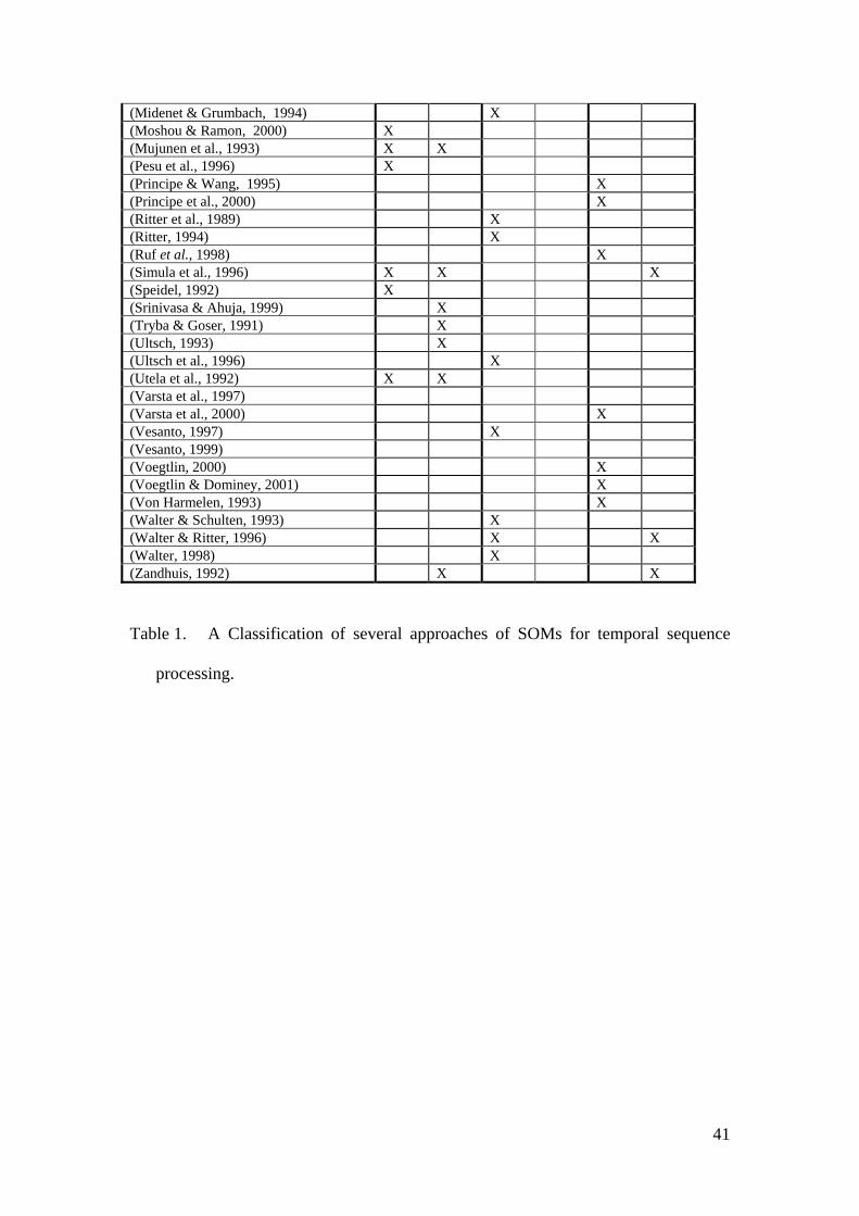
41
(Midenet & Grumbach, 1994) X (Moshou & Ramon, 2000) X (Mujunen et al., 1993) X X (Pesu et al., 1996) X (Principe & Wang, 1995) X (Principe et al., 2000) X (Ritter et al., 1989) X (Ritter, 1994) X (Ruf et al., 1998) X (Simula et al., 1996) X X X (Speidel, 1992) X (Srinivasa & Ahuja, 1999) X (Tryba & Goser, 1991) X (Ultsch, 1993) X (Ultsch et al., 1996) X (Utela et al., 1992) X X (Varsta et al., 1997) (Varsta et al., 2000) X (Vesanto, 1997) X (Vesanto, 1999) (Voegtlin, 2000) X (Voegtlin & Dominey, 2001) X (Von Harmelen, 1993) X (Walter & Schulten, 1993) X (Walter & Ritter, 1996) X X (Walter, 1998) X (Zandhuis, 1992) X X
Table 1. A Classification of several approaches of SOMs for temporal sequence
processing.

42
Fig. 1. A taxonomy of temporal SOM
Fig. 2. Temporal Sequence processing with a tapped delay as input for a SOM
Fig. 3. Temporal sequence processing using time-related transformations as pre-
processing for the SOM
Fig. 4. Structure of a trajectory based SOM
Fig. 5. Structure of the Kangas Map
Fig. 6. Structure of each unit in a Temporal Kohonen Map (TKM)
Fig. 7. Structure of each unit in a recurrent SOM
Fig. 8. Structure of the Recursive SOM
Fig. 9. Structure of each unit in a SOMTAD based map
Fig. 10. Structure of a Hierarchical SOM

43
Temporal SOM
Unmodified SOM
Modifiedlearning rule
Modifiedtopology
Tapped delay
Transformationbased
Embeddedtime
Trajectorybased
Hyper-map
Kangasmap Feedback Hierarchical
Level 0
Level 2
Level 1
Level 3Temporal Recurrent Recursive SOMTAD
Temporal SOM
Unmodified SOM
Modifiedlearning rule
Modifiedtopology
Tapped delay
Transformationbased
Embeddedtime
Trajectorybased
Hyper-map
Kangasmap Feedback Hierarchical
Level 0
Level 2
Level 1
Level 3Temporal Recurrent Recursive SOMTADTemporal Recurrent Recursive SOMTAD
44
Z-1
x(t-1)
x(t)
x(t-2)
Z-1
x(t-M) Z-1
X SOM

45
x(t) X SOMTime-related
transformation(ex. FFT)

46
b.m.u. t=1(best-match for t=1)
SOM
b.m.u. t=2 b.m.u. t=3 b.m.u. t=4
trajectory
b.m.u. t=1(best-match for t=1)
SOM
b.m.u. t=2 b.m.u. t=3 b.m.u. t=4
trajectory

47
last best-matchunits consideredfor next iteration
SOM
last best-matchunits consideredfor next iteration
SOM

48
Z-1
+
α
-
wi(n)
x(n) ||.|| Vi(n)y(n)
error
magnitudecomputationinput
unit weights
differencecomputation
leakyintergrator
final output
1−α
Z-1Z-1
+
α
-
wi(n)
x(n) ||.|| Vi(n)y(n)
error
magnitudecomputationinput
unit weights
differencecomputation
leakyintergrator
final output
1−α

49
Z-1
+
α
-
wi
x ||.|| Viy
errormagnitudecomputationinput
unit weights
differencecomputation
leakyintergrator
final output
feedback error
1-α
Z-1Z-1
+
α
-
wi
x ||.|| Viy
errormagnitudecomputationinput
unit weights
differencecomputation
leakyintergrator
final output
feedback error
1-α

50
x
SOM(map of units)
Vinput to the SOM
past activations
(x,V)
,
concatenationinput pattern
x
SOM(map of units)
Vinput to the SOM
past activations
(x,V)
,
concatenationinput pattern

51
TKMx
input TKM unit
β
intermediateactivation
Vi
Vneigh
activation ofneighbors
+
output

52
...
xinput
all or part of the data
...
all or part of the data
lower level SOMs
second level SOMs
(up to higher level SOMs)
......
xinput
all or part of the data
......
all or part of the data
lower level SOMs
second level SOMs
(up to higher level SOMs)
...