a technical note on index methodology enhancement by · pdf fileinclude various types of...

MIT/CRE – CREDL

A Technical Note on Index Methodology Enhancement by Two-stage

Regression Estimation

Supplement 1 to: A Set of Indexes for Trading Commercial Real Estate

Based on the Real Capital Analytics Transaction Prices Database

MIT Center for Real Estate Commercial Real Estate Data Laboratory - CREDL

David Geltner & Sheharyar Bokhari (MIT)

Release 1 April 21, 2008

Abstract: This technical supplement to the MIT/CRE Moody’s/REAL Indexes methodology white paper describes a second stage regression frequency conversion procedure which can be used to improve or supplement some of the Moody’s/REAL Indexes. After first estimating lower-frequency indexes staggered in time, a second-stage regression then applies a generalized inverse estimator to convert from lower to higher frequency return series. The two-stage procedure can improve the accuracy of high-frequency indexes in scarce data environments, and also can mitigate an errors-in-variables problem that arises at very high frequency even with plentiful data (e.g., monthly indexes). In this paper the method is described and analyzed via simulation analysis and by application to the empirical RCA repeat-sales data on which the Moody’s/REAL Indexes are based.

The proprietary indexes described in this white paper have been exclusively licensed to Real Estate Analytics LLC, and are produced and published by Moody’s Investors

Service as the Moodys/REAL Commercial Property Price Indexes.

MIT/CRE – CREDL

Table of Contents

Section Page

1. Background 1 2. General Purpose and Nature of the Methodology Enhancement 1 3. Two-stage Estimation & the Moore-Penrose Pseudoinverse 3 4. An Empirical Comparison of 2-stage versus Direct Estimation in Data-Scarce Markets

12 5. High Frequency Indexes and Errors-in-Variables 16 6. Conclusion 20 Appendix A: The Moore-Penrose Pseudoinverse or the Generalized Inverse A-1 Appendix B: A Note on Bias in the Moore-Penrose Frequency Conversion B-1 Appendix C: Charts of ATQ and DirQ for All 16 Moody’s/REAL Annual Indexes C-1 Bibliography R-1

MIT/CRE – CREDL

A Technical Note on Index Methodology Enhancement by Two-stage Regression Estimation

1. Background

This white paper describes an enhancement to the index computation

methodology which will be employed in some of the markets tracked by the Moody’s/REAL Commercial Property Price Indexes.

The regular production and publication of transaction price-based commercial

property price indexes of U.S. commercial property markets based on the Real Capital Analytics Inc (RCA) repeat-sales database commenced in December 2006, published at first on the MIT Center for Real Estate web site. These indexes are licensed to Real Estate Analytics LLC (REAL) and since October 2007 have been produced and published by Moody’s Investors Service as the Moody’s/REAL Commercial Property Price Indexes. The methodology of index computation was developed at the MIT/CRE, as described in a white paper first posted on the MIT/CRE web site in a release dated December 15, 2006. As noted in the white paper, the methodology for producing the indexes is to be updated and improved from time to time based on experience with the indexes and improvements available within the methodology. Some changes in the index production protocols were noted in a “Release 2” of the methodology white paper dated September 26, 2007. The present technical note describes an additional enhancement to the methodology in the form of a second-stage regression estimation which can serve two purposes: (i) to provide a way to derive supplementary quarterly-frequency indexes from the staggered annual returns reported in 16 of the 29 Moody’s/REAL index market segments; and (ii) to improve the high-frequency estimation in the Moody’s/REAL national aggregate monthly index.1 Present plans are to implement the second-stage regression enhancement for the national monthly index and as a supplement to the 16 annual-frequency indexes as of the reporting of the first returns of calendar year 2008 in the respective indexes.

2. General Purpose and Nature of the Methodology Enhancement

In the world of transaction price indexes used to track market movements in real estate, it is a fundamental fact of statistics that there is an inherent trade-off between the frequency of a price-change index and the amount of “noise” or “error” in the individual periodic price-change or “capital return” estimates.2 The major approach in the academic

1 A methodology for frequency conversion aimed in particular at the first of these two purposes was presented in Appendix D of “Release 2” of the methodology white paper dated September 26, 2007. While fundamentally similar to that methodology, the frequency conversion methodology presented in the present paper is an improvement upon the methodology described in the earlier white paper. (The earlier methodology was never implemented in the published Moody’s/REAL Indexes.) 2 The terms “noise” and “error” are used more or less interchangeably in this paper. They are placed in quotes here (though we won’t generally bother to do so subsequently in the paper) because these two words are used in their sense as statistical terms of art, not with the same meaning as they are often used in common parlance. The word “error” in this paper does not imply that there is any conceptual or

Moody’s/REAL Indexes White Paper, Supplement 1, Page 1

MIT/CRE – CREDL

real estate literature for addressing small-sample problems in price indexes is the ridge regression procedure, and this procedure is employed in the Moody’s/REAL indexes. Other approaches that have been explored in recent years in the academic literature include various types of parsimonious regression specifications that effectively parameterize the historical time dimension, as well as procedures that make use of temporal and spatial correlation in real estate markets.3 Some such techniques show promise, but are perhaps more appropriate in the housing market than in commercial property markets. Spatial correlation is more straightforward in housing markets, and the need for transparency in a tradable index can make it problematical to estimate the index on sales outside of the subject market segment. Another concern that is of particular importance in indexes supporting derivatives trading is that the index estimation procedure should minimize the constraints placed on the temporal structure and dynamics of the estimated returns series, allowing each consecutive periodic return estimate to be as independent as possible, in particular so as to avoid lag bias and to capture turning points in the market even if these are inconsistent with prior temporal patterns in the index.4

The present paper describes a two-stage estimation procedure in which, after a

first-stage regression is run to optimize the index at a sufficiently low frequency to eliminate most noise (recognizing the scarce data environment), a second-stage regression is performed to convert a staggered series of such low-frequency indexes to a higher-frequency index. The procedure is optimal in the sense that it minimizes additional (second stage) noise and does not introduce artificial index price lag bias or smoothing (as would be the case with simple smoothing or rolling techniques, and with some of the time-parameterization techniques noted earlier).5

While the resulting high-frequency index does not have as high a signal/noise

ratio (SNR) as the underlying low-frequency indexes, it can have a higher SNR than direct high-frequency estimation, with the advantage of the greater utility of the higher frequency. This suggests that it may be useful in the information marketplace to publish both the staggered low-frequency indexes and the higher-frequency second-stage derived index as supplemental information, either alone or along with directly-estimated high-frequency indexes, at least in markets where data is too scarce to rely solely on directly-estimated high-frequency indexes.

computational mistake or that anyone has done anything wrong, and the word “noise” does not imply that the index makes any sound (obviously!). 3 See, for example, Schwann (1998), McMillen & Dombrow (2001), and Clapp (2004), among others. A recent overview is in Pace & LeSage (2004). 4 This is particularly important to allow the derivatives to hedge the type of risk that traders on the short side of the derivatives market are typically trying to manage. For example, developers or investment managers seek to hedge against exposure to unexpected and unpredictable turning points or movements in the commercial property market. 5 While in the Moody’s/REAL Indexes the second-stage frequency conversion is applied to repeat-sales indexes estimated at the lower frequency, in principle the 2-stage procedure can be applied with any methodology for estimating the first-stage (lower-frequency) indexes as long as the lower-frequency estimation can be staggered regularly in time.


MIT/CRE – CREDL

Furthermore, in the case of very high frequency indexing, such as monthly frequency, the two-stage procedure also helps to address an errors-in-variables problem in the time dummy-variables that are used to estimate longitudinal indexes. This problem arises from the fact that, even though the closing dates of transactions may be observed with very high accuracy, the time lapse between when the economic pricing decision was made and when the closing occurred is typically a difficult-to-observe length of time that varies randomly across transactions over a range of perhaps several weeks, enough to cause errors-in-variables at the monthly frequency. Thus, for monthly indexes the two-stage/frequency-conversion approach may be valuable even where data scarcity is not an issue and the high-frequency index can stand alone.

3. Two-stage Estimation & the Moore-Penrose Pseudoinverse In this section we will introduce the two-stage/frequency-conversion procedure from the perspective of increasing index frequency in a data-scarce environment, in particular, for deriving a supplemental quarterly-frequency index from four underlying staggered annual-frequency indexes. It is well known that commercial property transaction price data is scarce compared to housing data. To the extent the market wants to trade specific segments, such as, say, New York office buildings or Southern California retail properties, the transaction sample becomes so small that we have deemed that within the current RCA database it is necessary to accumulate a full year’s worth of data before we have enough repeat-sales observations to produce a good transactions-based estimate of the price movement experienced by investors. This is the type of context in which the following two-stage/frequency-conversion procedure may be used to produce a quarterly index.

3.1 The Methodology: We begin by estimating annual indexes in four versions with quarterly staggered

starting dates, beginning in January, April, July, and October. We label these four annual indexes as “CY”, “FYM”, “FYJ”, and “FYS” to refer to “calendar years” and “fiscal years” identified by their ending months. Each index is a true annual index, not a rolling or moving average within itself, but consisting of independent consecutive annual returns.6 The result will look something like what is pictured in Exhibit 1 for an example index based on the Real Capital Analytics repeat-sales database for Southern California (Los Angeles & San Diego) retail property.7 If properly specified, these annual indexes

6 That is, independent within each index. Obviously, there is temporal overlap across the indexes. 7 The annual indexes shown in Exhibit 1 differ slightly from the “official” Moody’s/REAL Indexes for Southern California retail. For research analysis purposes to develop the enhanced methodology we employ fully-updated indexes, and these are pictured in Exhibit 1 (and elsewhere in this paper). The difference with the official Moody’s/REAL Indexes is that the latter are meant to represent only the realized price change experiences of investors who have cashed out by the time each index report is published. Therefore, the official indexes are effectively “frozen” after each period’s report, without backward adjustment to the prior history.


MIT/CRE – CREDL

have essentially no lag bias.8 Each of these indexes also has as little noise as is possible given the amount of data that can be accumulated over the annual spans of time.9

Exhibit 1: (CY is the calendar year index ending December 31 each year, FYM is the index ending March 31 each year, FYJ is the index ending June 30 each year, and FYS is the index ending September 30 each year.)

Southern CA Retail:Four Staggered Annual Indexes (set to starting value 1.0 at first observation)

0.8

1

1.2

1.4

1.6

1.8

2

2.2

2.4

2.6

4Q 2

000

1Q 2

001

2Q 2

001

3Q 2

001

4Q 2

001

1Q 2

002

2Q 2

002

3Q 2

002

4Q 2

002

1Q 2

003

2Q 2

003

3Q 2

003

4Q 2

003

1Q 2

004

2Q 2

004

3Q 2

004

4Q 2

004

1Q 2

005

2Q 2

005

3Q 2

005

4Q 2

005

1Q 2

006

2Q 2

006

3Q 2

006

4Q 2

006

1Q 2

007

2Q 2

007

3Q 2

007

4Q 2

007

CY FYM FYJ FYS

Next, a frequency-conversion is applied to this suite of annual-frequency indexes to obtain a quarterly-frequency price index implied by the four staggered annual indexes. We want to perform this frequency conversion in the most accurate way possible, with as little additional noise and bias as possible. How can we use those staggered annual indexes to derive an up-to-date quarterly-frequency index? Looking at the staggered

8 Time-weighted dummy variables are used to eliminate temporal aggregation. For example, for the calendar year (CY) index beginning January 1st, a repeat-sale observation of a property that is bought September 30 2004 and sold September 30 2007 has time-dummy values of zero prior to CY2004 and subsequent to CY2007, and dummy-variable values of 0.25 for CY2004, 1.0 for CY2005 and CY2006, and 0.75 for CY2007. This specification, attributable to Bryon & Colwell (1982), eliminates the averaging of the values across the years, and pegs the returns to end-of-year points in time. For more details, see the basic MIT methodology white paper, Geltner & Pollakowski (2007). 9 A noise filter such as ridge regression can be helpful in this regard (as introduced into the real estate literature by Goetzmann, 1992), and has in fact been used in the indexes shown. As noted, the two-stage procedure does not constrain the methodology used to estimate the lower-frequency indexes, and various procedures might be employed to optimize the estimation of the lower-frequency indexes.


MIT/CRE – CREDL

annual-frequency index levels pictured in Exhibit 1, one is tempted to try to construct a quarterly-frequency index by simply averaging across the levels of the four indexes at each point in time. (Try to fit a curve “between” the four index levels.) But such a process would entail a delay of three quarters in computing the most recent quarterly return (while we accumulate all four annual indexes spanning that quarter), which for derivatives trading purposes would defeat the purpose of the higher-frequency index. Such a levels-averaging procedure would also considerably smooth the true quarterly returns (it would effectively be a time-centered rolling average of the annual returns).

The approach we employ for the frequency-conversion procedure is a second-

stage “repeat-sales” regression at the quarterly frequency using the four staggered annual indexes as the input data. Each annual return on each of the four staggered indexes is treated as a “repeat-sale” observation in this second-stage regression. If we have T years of history, we will have 4T-3 such “repeat-sales” observations (the row dimension of the second-stage regression data matrix), and we will have 4T quarters for which we have time-dummies (the columns dimension in the regression data matrix, the quarters of history for which we want to estimate returns). We are missing “1st-sales” observations for the first three quarters of the history, the quarters that precede the starting dates for all of the annual indexes other than the one that starts earliest in time (the CY index in our present example), as the staggered annual indexes each must start one quarter after the previous. Obviously, with fewer rows than columns in the estimation data matrix, our regression is “under-identified”, that is, the system has fewer equations than unknowns.10 Basic linear algebra tells us that such a system has an infinite number of exact solutions (that is, quarterly index return estimates that will cause the predicted values to exactly match the “repeat-sales” observations on the left-hand-side of the second-stage regression, i.e., a regression R2 of 100%, a perfect fit to the data, the low-frequency index returns). However, of all of those infinite solutions, there is a particular solution that minimizes the variance of the estimated parameters, i.e., that minimizes the additional noise in the quarterly returns, noise added by the frequency-conversion procedure. This solution is obtained using what is called the “Moore-Penrose pseudoinverse” matrix of the data. This solution is “best” in the sense that it has the least variance (is most “precise”) and the least bias possible for a linear estimator. We shall refer to this frequency-conversion method as the “Moore-Penrose Generalized Inverse Estimator”, or MPGIE for short.11

How good is the MPGIE as a frequency-conversion method? For practical

purposes, it is quite good. It adds effectively very little noise or bias to the annual returns. This can be seen by numerical simulation. Exhibit 2 depicts a typical randomly-generated history of true quarterly market values (the thick black line, which in the real world 10 We cannot simply drop out the first three quarters from the second-stage index, as that will then impute the first three annual returns to their respective quarters and thereby bias the estimation of all of the quarterly returns. 11 See Appendix A for an introduction to the Moore-Penrose pseudoinverse and its role in solving the under-identified system. See Appendix B for a discussion of bias in the resulting estimator. As noted in Appendix A, it can be shown that, while the Moore-Penrose pseudoinverse estimator of the under-identified system is biased, the bias is minimized among the class of linear estimators (Chipman, 1964). That is, the Moore-Penrose is “Best Linear Minimum Bias Estimator” (BLMBE).


MIT/CRE – CREDL

would be unobservable), the corresponding staggered annual index levels (thin, dashed lines, here without any noise, to reveal the noise added purely by the frequency-conversion second stage), and the resulting second-stage MPGIE-estimated quarterly index levels (thin red line with triangles, labeled “ATQ” for “Annual-to-Quarerly”).12 Clearly, the derived MPGIE quarterly index almost exactly matches the true quarterly market value levels. Numerous simulations of random histories and varying market patterns over time give similar results to those depicted in Exhibit 2. The MPGIE-based frequency-conversion in itself appears to add only a little noise or bias to the staggered annual indexes.

Exhibit 2: True vs Estimated Underlying Staggered Annual Indexes (simulation) True vs Estimated vs Underlying Staggered Annual Indexes (simulation)

0.5

0.7

0.9

1.1

1.3

1.5

1.7

0 2 4 6 8 10 12 14 16 18 20 22 24 26

Period

TRUE Estd ATQ CY FYM FYJ FYS

12 In Exhibit 2 the first (CY) annual index starts arbitrarily at a value of 1.0, and the subsequent three staggered annual indexes are pegged to start at the interpolated level of the just-prior annual index at the time of the subsequent index’s start date. This is merely a convention and does not impact the quarterly return estimates, as all indexes are only indicators of relative price movements across time, not absolute price levels.


MIT/CRE – CREDL

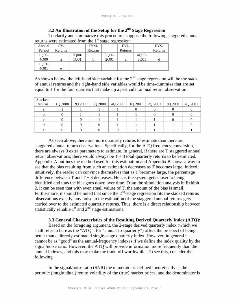
3.2 An Illustration of the Setup for the 2nd Stage Regression To clarify and summarize this procedure, suppose the following staggered annual

returns were estimated from the 1st stage regression: Annual Period

CY-Returns

FYM-Returns

FYJ-Returns

FYS-Returns

1Q00-4Q00 a

2Q00-1Q01 b

3Q00-2Q01 c

4Q00-3Q01 d

1Q01-4Q01 e

As shown below, the left-hand side variable for the 2nd stage regression will be the stack of annual returns and the right-hand side variables would be time-dummies that are set equal to 1 for the four quarters that make up a particular annual return observation. Stacked-Returns 1Q 2000 2Q 2000 3Q 2000 4Q 2000 1Q 2001 2Q 2001 3Q 2001 4Q 2001

a 1 1 1 1 0 0 0 0 b 0 1 1 1 1 0 0 0 c 0 0 1 1 1 1 0 0 d 0 0 0 1 1 1 1 0 e 0 0 0 0 1 1 1 1

As seen above, there are more quarterly returns to estimate than there are

staggered annual return observations. Specifically, for the ATQ frequency conversion, there are always 3 extra parameters to estimate. In general, if there are T staggered annual return observations, there would always be T + 3 total quarterly returns to be estimated. Appendix A outlines the method used for this estimation and Appendix B shows a way to see that the bias resulting from such an estimation decreases as T becomes large. Indeed, intuitively, the reader can convince themselves that as T becomes large, the percentage difference between T and T + 3 decreases. Hence, the system gets closer to being identified and thus the bias goes down over time. From the simulation analysis in Exhibit 2, it can be seen that with even small values of T, the amount of the bias is small. Furthermore, it should be noted that since the 2nd-stage regression fits the stacked returns observations exactly, any noise in the estimation of the staggered annual returns gets carried over to the estimated quarterly returns. Thus, there is a direct relationship between statistically reliable 1st and 2nd stage estimations.

3.3 General Characteristics of the Resulting Derived Quarterly Index (ATQ): Based on the foregoing argument, the 2-stage derived quarterly index (which we

shall refer to here as the “ATQ”, for “annual-to-quarterly”) offers the prospect of being better than a directly-estimated single-stage quarterly index. However, in general it cannot be as “good” as the annual-frequency indexes if we define the index quality by the signal/noise ratio. However, the ATQ will provide information more frequently than the annual indexes, and this may make the trade-off worthwhile. To see this, consider the following.

In the signal/noise ratio (SNR) the numerator is defined theoretically as the

periodic (longitudinal) return volatility of the (true) market prices, and the denominator is


MIT/CRE – CREDL

defined as the standard deviation in the estimated periodic return.13 The MPGIE frequency-conversion procedure gives a SNR denominator for the ATQ which is not much larger than that of the underlying annual-frequency indexes (the standard deviation of the second-stage quarterly return estimate not much larger than that in the first-stage annual return estimates, as evident in the simulation depicted in Exhibit 2 by the fact that the ATQ adds very little error). But the numerator of the SNR is governed by the fundamental dynamics of the (true) real estate market. These dynamics dictate that the periodic return volatility will be smaller for higher frequency returns. For example, if the market follows a random walk (serially uncorrelated returns), the quarterly volatility will be 1/SQRT(4) = 1/2 the annual volatility. This means that, even if the SNR denominator did not increase at all, the SNR in the ATQ would be one-half that in the underlying annual indexes. If the market has some sluggishness or inertia (positive autocorrelation in the quarterly returns) then the SNR will be even more reduced in the ATQ below that in the annual indexes.

Importantly, the SNR of the 2-stage ATQ can still be greater than that of a

directly-estimated (single-stage) quarterly index. To see this, suppose price observations occur uniformly over time. Then there will be four times as much data for estimating the typical annual return in the annual-frequency indexes compared to the typical quarterly return in the directly-estimated quarterly-frequency index. By the basic “Square Root of N Rule” of statistics, this implies that the directly-estimated quarterly index will tend to have SQRT(4) = 2 times greater standard error in its (quarterly) return estimates than the annual indexes have in their (annual) return estimates. Thus, the SNR for the direct quarterly index will have a denominator twice that of the annual indexes. This compares to the 2-stage ATQ whose SNR denominator may be only slightly greater than in the annual indexes (as was suggested in the previous section, depicted in Exhibit 2). Of course, either way of producing a quarterly index will still be subject to the same numerator in the theoretical SNR, which is purely a function of the true market volatility. Thus, while the 2-stage ATQ will have a lower SNR than the underlying annual-frequency indexes, it may have a higher SNR than a directly-estimated (1-stage) quarterly index. In data-scarce situations, this can make an important difference.14

13 The theoretical SNR cannot be observed or quantified in the real world, where the true market returns cannot be observed, and hence the true market volatility (SNR numerator) cannot be observed. Empirical estimates of the theoretical SNR are confounded by the fact that the volatility of any empirically estimated index will include the effect of the noise in the estimated index. Furthermore, the denominator of the theoretical SNR should equal the theoretical standard deviation within each return estimate, which is not exactly what is measured by the regression’s standard errors of its coefficients. (To see this, consider conceptually a “perfect” index whose return estimate always exactly equal the unobservable true market return each period. The regression producing such an index would still have positive standard errors for its coefficients for any finite repeat-sale sample, as there is noise in the estimation database, causing the regression to have non-zero residuals.) In spite of these practical limitations, the theoretical SNR is a useful construct for conceptual analysis purposes (and also in simulation analysis, where “true” returns can be simulated and observed). 14 Formal definition and computation of the standard error for the MPGIE second-stage regression is not straightforward, and is not attempted here. It is not clear how to define such a metric in a manner that would be practical for empirical computation with real world indexes and that would also be meaningful for our purposes. A key problem is that the standard error of the regression residuals does not generally


MIT/CRE – CREDL

It is also important to note that, while the ATQ does not have as good SNR as the

annual indexes, it does provide more frequent returns than the annual indexes (quarterly instead of annual), and thereby does provide additional information.15 Thus, there is a useful trade-off between the staggered annual indexes and the derived ATQ: the ATQ gives up some SNR information usefulness in the accuracy of its return estimates, but in return provides higher frequency return information.

This trade-off suggests that it may make sense in practical applications to produce

and publish both the staggered annual indexes and their implied MPGIE-based ATQ quarterly index. Whether the real estate derivatives market will want to actually trade contracts written on the ATQ is a question that only the market can decide. But in any case the ATQ will provide information useful to market participants and analysts.16

3.4 An Illustrative Example of Annual-to-Quarterly Derivation in Data-Scarce Markets: To gain a more concrete feeling for the above-described methodology and

application, consider two of the smaller (and therefore more data-scarce) markets among the 29 Moody’s/REAL Commercial Property Price Index market segments: New York office properties, and Southern California retail properties.17

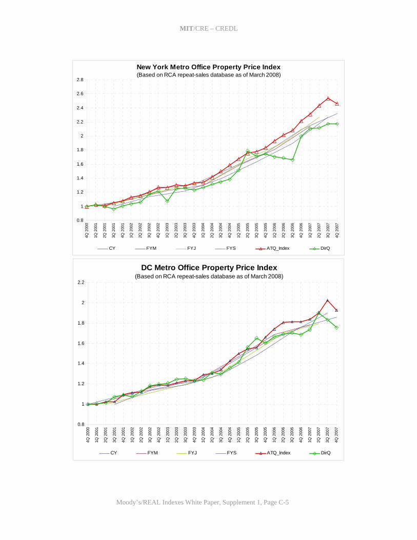
The New York office index is a good one to see the difference that can occur

between direct quarterly estimation and the 2-stage ATQ. Exhibit 3 shows these two alternative ways to estimate a quarterly-frequency index. Even though noise filtering is used in the direct quarterly estimation, this index (indicated by the green line with diamonds) is clearly quite noisy, and differs markedly from the staggered annual indexes estimated from the same repeat-sales data.18 The direct quarterly index does not well represent what was going on in the New York metro region office market during the 2001-2007 period, especially in the index’s sharp downtick in 2003Q1 and its long price correspond to the type of “error” that is meaningful in a price index, which is the standard deviation of the estimate of the coefficient (each individual return). 15 Among the four staggered annual indexes we do get new information every quarter, but that information is only for the entire previous 4-quarter span, which is not as useful as information about the most recent quarter itself, which is what is provided by the ATQ. For example, a turning point in the most recent quarter will not necessarily show up in the most recent annual index, as the latter is still influenced by market movement earlier in the 4-quarter span it covers. 16 If derivative contracts are to be written on the ATQ or other directly-estimated quarterly-frequency indexes, it may well be advisable to have contract payment settlement be based on a rolling average of the high-frequency returns. For example, the settlement of the payments owed based on quarter t’s return might be based ultimately on an average of the returns in quarters t-1 and t, or perhaps on three quarters: t-1, t, and t+1. 17 These two markets are selected here because they are representative of both the strengths and weaknesses of the 2-stage procedure. During the 2005-07 period the New York Office index averaged 25 transaction price observations (second-sales) per quarter, while the Southern California (Los Angeles & San Diego MSAs) index averaged 24 observations/quarter. 18 In Exhibit 3 the staggered annual indexes are all presented with the convention of starting at a value of unity (as in Exhibit 1, but in contrast to Exhibit 2). All indexes in Exhibit 3 (as within each of the subsequent exhibits) are estimated from the same repeat-sales database, namely, all RCA second-sales prior to the end of 2007Q4 and available in the database as of mid-March 2008.


MIT/CRE – CREDL

slide from 2005Q2 through 2006Q3, a period which casual observation and the trade press would seem to indicate was one of robust growth in the New York office market. The staggered annual indexes and the ATQ do much better in representing the strong bull market of that period, and indeed in this particular case the ATQ seems to be about as good as the annual indexes, in addition to being more frequent. Note in particular the downturn in 2007Q4 picked up by the ATQ but not yet apparent in the annual indexes, a downturn consistent with the credit crunch of late 2007.

Exhibit 3: New York office property price index based on RCA repeat-sales database, directly estimated (green diamonds) and derived ATQ (red triangles), together with the staggered annual indexes: 2001Q1-2007Q4.

New York Metro Office Property Price Index(Based on RCA repeat-sales database as of March 2008)

0.8

1

1.2

1.4

1.6

1.8

2

2.2

2.4

2.6

2.8

4Q 2

000

1Q 2

001

2Q 2

001

3Q 2

001

4Q 2

001

1Q 2

002

2Q 2

002

3Q 2

002

4Q 2

002

1Q 2

003

2Q 2

003

3Q 2

003

4Q 2

003

1Q 2

004

2Q 2

004

3Q 2

004

4Q 2

004

1Q 2

005

2Q 2

005

3Q 2

005

4Q 2

005

1Q 2

006

2Q 2

006

3Q 2

006

4Q 2

006

1Q 2

007

2Q 2

007

3Q 2

007

4Q 2

007

CY FYM FYJ FYS ATQ_Index DirQ


MIT/CRE – CREDL

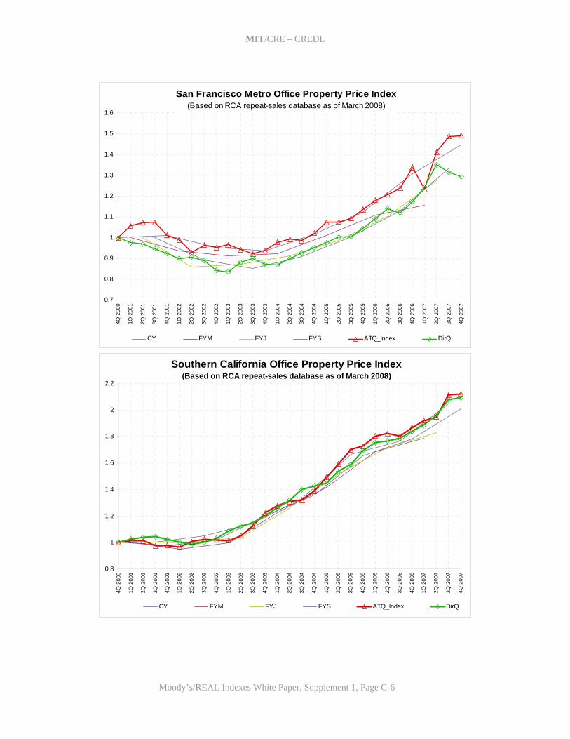
The Southern California (Los Angeles and San Diego metro areas) retail property

index is a good one to see how the ATQ works, including both its strengths and weaknesses. Exhibit 4 depicts the MPGIE-based ATQ (solid red line with triangles) superimposed on its underlying staggered annual indexes (the same as were presented in Exhibit 1) for the 2001Q1-2007Q4 period.

Exhibit 4: MPGIE-based ATQ for Southern California retail property, 2001Q1-2007Q4, superimposed on the underlying staggered annual indexes (same as Exhibit 1).

Southern California Retail Property Price Index(Based on RCA repeat-sales database as of March 2008)

0.8

1

1.2

1.4

1.6

1.8

2

2.2

2.4

2.6

2.8

4Q 2

000

1Q 2

001

2Q 2

001

3Q 2

001

4Q 2

001

1Q 2

002

2Q 2

002

3Q 2

002

4Q 2

002

1Q 2

003

2Q 2

003

3Q 2

003

4Q 2

003

1Q 2

004

2Q 2

004

3Q 2

004

4Q 2

004

1Q 2

005

2Q 2

005

3Q 2

005

4Q 2

005

1Q 2

006

2Q 2

006

3Q 2

006

4Q 2

006

1Q 2

007

2Q 2

007

3Q 2

007

4Q 2

007

CY FYM FYJ FYS ATQ_Index

In the Exhibit, note how the ATQ is generally consistent with the annual returns that span each quarter. However, the quarterly index picks up the changes implied by changes in the staggered annual indexes. For example, while the FYS annual index ending in 2006Q4 was positive, it was less positive than the immediately preceding FYJ annual index ending in 2006Q3. (The FYS ending in 2006Q4 was up 4.6% but the FYJ ending in 2006Q3 was up 17.4%.) The resulting derived ATQ quarterly index indicated a downturn in 2006Q4 (-2.4%).

At first it may seem odd that the derived quarterly index can be negative when the

annual indexes that span the quarter are all positive. The intuition behind a result such as the above example is that a subsequent annual index could still be increasing as a result of rises during the first 3 quarters of its 4-quarter time-span, with a drop in the last quarter that does not wipe out all of the previous three quarters’ gains. For example, suppose the


MIT/CRE – CREDL

following are the true quarterly changes during the past 5 quarters: 07Q1 = +3%, 07Q2 = +3%, 07Q3 = +3%, 07Q4 = +3%, 08Q1 = -4%. Then the CY07 annual index would show +12% (ending 12/31/07), and the FYM08 annual index would show +5% (ending 3/31/08), even though the 08Q1 quarterly return is negative. When the most recent annual index is rising at a lower rate than the next-most-recent annual index, it can (although does not necessarily) indicate that the most recent quarter was negative. The derived quarterly return (ATQ) methodology is designed to discover and quantify such situations as best we can. As noted, simple curve-fitting of the annual indexes introduces considerable smoothing, and will not be able to pick up in a timely manner the kind of turning points we have just described.

On the other hand, as we previously noted, the ATQ will have a lower

signal/noise ratio than the underlying staggered annual return indexes from which it is derived. The result can be that each individual quarterly return is more prone to noise, possibly less accurate, than is the case for each of the annual returns in the annual-frequency indexes.19 For example, in Exhibit 4, look at the ATQ return for 2007Q2. The ATQ indicates a huge uptick in that quarter of 10.9%. While the second quarter of 2007 was indeed the last period of the great bull market, it seems unlikely that Southern California retail property market values really increased that much in a single quarter. The ATQ estimate of 10.9% may indeed make mathematical sense given that the FYJ annual index ending at the end of 2007Q2 rose 7.1% after the previous FYM annual index ending at the end of 2007Q1 actually declined by 3.5%. But those annual indexes are not without noise, and the effect of that noise may appear exaggerated in the ATQ estimate for 2007Q2.

4. An Empirical Comparison of 2-stage versus Direct Estimation in Data-Scarce Markets

The preceding section presented a concrete example of both the strengths and

weaknesses of the 2-stage/frequency-conversion procedure for providing supplemental higher-frequency asset price-change information in small markets. We have suggested that the 2-stage procedure may tend to be better than direct (single-stage) high-frequency estimation, although we have not formalized that argument. Whether single-stage or two-stage estimation is more accurate depends on whether the second stage of regression adds less noise (and bias) than is removed by the effective increase in sample size presented by the longer return period intervals in the staggered lower-frequency estimation in the first of the two stages. This may ultimately be an empirical question, and even if the 2-stage procedure does tend generally to be more accurate than direct high-frequency estimation, either procedure may be more accurate in a given specific empirical instance. In any case, the specific “errors” will differ across the two techniques, which suggests that there may be benefit in the information marketplace in producing and publishing both types of high-frequency indexes.

19 This is why we suggested in a previous note that if trading is to be done on quarterly indexes the contracts might consider settling on a moving average of adjacent quarterly returns.


MIT/CRE – CREDL

In this section we present an empirical comparison of the two approaches. As noted, computation of index estimated returns standard errors is not straightforward for the ATQ, and “apples-to-apples” comparisons of estimated standard errors across the two procedures is not attempted in the present paper.20 However, there are two statistical characteristics of an estimated real estate asset market price index that can provide practical, objective information about the quality of the index. These two characteristics are the volatility and the first-order autocorrelation of the index’s estimated returns series. Based on statistical considerations, we know that noise in the index returns will tend to increase the observed volatility in the index returns. And we know that noise will also tend to drive the index returns’ first-order autocorrelation down, toward negative 50%.21

Considering the foregoing, it would seem reasonable to compare the two index

estimation methodologies based on the volatilities and first-order autocorrelations of the resulting estimated historical indexes. Lower volatility, and higher first-order autocorrelation, would be indicative of a “superior” index, that is, one that is likely to have less noise in its returns. For example, in the New York Office index that we considered in previously in Exhibit 3, the 2-stage ATQ index has 2.5% quarterly volatility, versus 6.8% in the directly-estimated (“DirQ”) index that seemed inferior. On the other hand, the Southern California Retail index that we considered in Exhibit 4 as an example of noise in the ATQ has first-order autocorrelation of -22%, well below what is likely realistic in the actual real estate asset market.

Among the Moody’s/REAL Commercial Property Price Indexes there are 16

indexes (including the New York Office and Southern California Retail indexes we have previously examined) that have been originally published at only the annual frequency (with four staggered versions, as described above), because the available transaction price data has been deemed to be insufficient to support quarterly estimation. An examination of the relative values of the quarterly volatilities and first-order autocorrelations resulting from estimation of quarterly indexes by the two alternative procedures across these 16 market segments can provide a quantitative comparison of the two procedures.

Exhibit 5 summarizes the quantitative comparison of the two quarterly index

procedures (labeled “ATQ” and “DirQ” in the exhibit) based on the volatilities and first-order autocorrelations. The volatility test is defined by the ratio of the ATQ volatility divided by the DirQ volatility. The autocorrelation test is defined by the difference between the ATQ first-order autocorrelation minus that of the DirQ. Both tests are applied separately to the entire 28-quarter available history 2001-2007 and to the more recent 12-quarter period 2005-07. The RCA repeat-sales database “matured” to a considerable degree by 2005, with many more repeat-sales observations available since that time. The comparison is made for each of the 16 indexes and also averaged across

20 For one thing, consider that the second-stage regression itself has no residuals, as it makes a perfect fit to the staggered lower-frequency indexes that are its dependent variable. Furthermore, as noted, the objective of a price index regression is not, in principle, the minimization of transaction price residuals per se, but rather the minimization of error in the coefficient estimates (the index’s periodic returns). 21 These are basic characteristics of the statistics of indexes. (See, e.g., Geltner & Miller et al (2007), Chapter 25.)


MIT/CRE – CREDL

the eight MSA-level and eight regional-level indexes. The overall impression left by this comparison is that neither quarterly index estimation method clearly dominates over the other. The ATQ procedure does seem to be slightly better, “winning” in more instances and in the overall averages. However, the DirQ procedure is superior in almost as many cases. In most markets, the two procedures are similar and any advantage seems to be slight.

Exhibit 5: Comparison of 16 quarterly indexes in data-scarce markets: 2-stage (“ATQ”) versus direct quarterly (“DirQ”), based on Volatility and Autocorrelation Tests. Index Comparison: 2-stage vs direct quarterly estimation:

Data*: Vol Test**: AC(1) Test***: MSA-level indexes: Index: 2005-07 2001-07 2005-07 2001-07NY Office 25 0.33 0.37 3% 21%DC Office 19 0.67 0.76 -28% -18%SF Office 17 1.52 1.32 -57% -48%SC Office 36 1.52 1.34 8% -14%SC Industrial 38 0.43 0.50 23% 44%SC Retail 24 1.06 0.99 -25% -15%SC Apts 58 1.20 1.02 -6% -12%FL Apts 36 0.70 0.60 82% 85%Average: 31 0.93 0.86 0% 5%Regional-level indexes: Index: 2005-07 2001-07 2005-07 2001-07E Office 70 0.39 0.54 -25% -10%S Office 52 0.79 0.82 51% 29%E Industrial 42 0.42 0.54 -5% 16%S Industrial 28 1.12 1.46 -32% 3%E Retail 33 0.63 0.58 -36% -18%S Retail 45 0.57 0.54 32% 23%E Apts 69 1.07 1.50 -46% -10%S Apts 83 0.84 0.58 21% 68%Average: 31 0.73 0.82 -5% 13%*Avg number of 2nd-sales obs/qtr 2005-07. Database was “immature” with considerably fewer 2nd-sales observations prior to 2005. ** Ratio of ATQ volatility/DirQ volatility: <1 ==> ATQ better; >1 ==> DirQ better. *** Difference: AC(1)ATQ - AC(1)DirQ. >0 ==> ATQ better; <0 ==> DirQ better.

The worst case for the ATQ procedure (and best, relatively speaking, for the DirQ

procedure) is the San Francisco Office index, which is shown for both the ATQ and the DirQ estimation in Exhibit 6 (along with the underlying staggered annual-frequency indexes). While the ATQ index for San Francisco offices seems slightly inferior to the DirQ index a several ways (e.g.: unlikely small upsurge in the period of the “tech bust” in early 2001; lack of a downturn in the second half of 2007), the biggest problem with the ATQ results from a single quarter, 2007Q1, in which the ATQ somehow derives an


MIT/CRE – CREDL

anomalous downturn of -7.8% (the DirQ is positive 5.9% in that quarter). The ATQ downturn is understandable in the underlying annual-frequency indexes: the CY index turned in a +16.5% return CY 2006, followed by the FYM index reporting only a +4.3% return for the four quarters ending in 2007Q1. But a little bit of positive noise in the CY2006 return followed by a little negative noise in the subsequent FYM return was apparently exaggerated in the ATQ derivation for 2007Q1. This is therefore an example where the DirQ procedure provided an effective “cross-check” on the ATQ procedure. (Counter-examples can also be found, e.g., as described previously for the New York office index shown in Exhibit 3).

Exhibit 6: San Francisco office property price index based on RCA repeat-sales database, directly estimated (green diamonds) and derived ATQ (red triangles), together with the staggered annual indexes: 2001Q1-2007Q4.

San Francisco Metro Office Property Price Index(Based on RCA repeat-sales database as of March 2008)

0.7

0.8

0.9

1

1.1

1.2

1.3

1.4

1.5

1.6

4Q 2

000

1Q 2

001

2Q 2

001

3Q 2

001

4Q 2

001

1Q 2

002

2Q 2

002

3Q 2

002

4Q 2

002

1Q 2

003

2Q 2

003

3Q 2

003

4Q 2

003

1Q 2

004

2Q 2

004

3Q 2

004

4Q 2

004

1Q 2

005

2Q 2

005

3Q 2

005

4Q 2

005

1Q 2

006

2Q 2

006

3Q 2

006

4Q 2

006

1Q 2

007

2Q 2

007

3Q 2

007

4Q 2

007


We conclude this analysis of the MPGIE-based 2-stage/frequency-conversion procedure application to data-scarce markets with the general suggestion that the procedure can add value. What we were here labeling the ATQ index appears to be generally at least as good as direct quarterly estimation, and capable of adding information that the marketplace may be able to use. However, in data-scarce environments such as examined here (e.g., second-sales observational frequency averaging in the mid-20s per quarter), the ATQ is best used as a supplement to annual-frequency indexes, not a replacement, and indeed the ATQ may itself also be


MIT/CRE – CREDL

supplemented by direct quarterly estimation, as the two procedures will tend to display “different noise”, and therefore will tend to complement each other, each serving as a “cross-check” on the other.22 5. High Frequency Indexes and Errors-in-Variables We noted in Section 1 that the two-stage/frequency-conversion procedure has two applications that are potentially of use in the Moody’s/REAL Indexes. In addition to the supplemental index reporting frequency enhancement that we have examined in the previous two sections, a second function applies not in particular to data-scarce environments, but rather to what are, in the real estate world, “high frequency” indexes; for practical purposes, the monthly frequency. At this frequency, the two-stage procedure can address a type of errors-in-variables problem that arises with the monthly time-dummy variables.

The nature of real estate transaction price data is that it is often possible to observe with a high degree of accuracy the date of the closing of the transaction. This observation of necessity becomes the date that governs the valuation of the monthly time-dummy variable associated with each transaction observation in the estimation of a price index. For example, consider the classical zero/one repeat-sale regression specification where the time-dummy coefficients are the index’s periodic returns estimates. For a given observation, all of the monthly time-dummies from the month after the month of the first sale closing date up through (including) the month of the second sale closing date, will take on values of unity, and all other months’ time-dummies will be set to zero for that repeat-sale observation. It has often been noted that there is a lag between the time when the actual, effective (economic) pricing decision was made for a given transaction and the subsequent closing date for that transaction. This lag obviously causes a type of lag in the index, in the sense that while the index measures returns based on realized closing dates, it is lagged behind pricing agreement dates. If the market effectively turns in September as reflected in prices agreed in deals struck in that month, but those deals do not close until November, then the index will not reflect the market turn until its report of the November return. Such a lag can be easily understood and dealt with in a derivatives market. But there is another, more subtle, problem.

The time lag between the effective price agreement date in the deal and the

subsequent closing date varies randomly across transaction observations. It is this random variation in the closing lag that can cause a right-hand-side errors-in-variables effect in the regression estimation. While the time-dummy variables are observed with high accuracy for closing times, they reflect randomly-varying lags in relation to the actual (effective) price agreement times. It is well known that this type of errors-in-variables can cause attenuation bias in coefficient estimates, that is, a bias toward zero in the estimated

22 Again, if contracts are to be written on such quarterly-frequency indexes, it may well be advisable to base settlement on averages of returns, either across adjacent quarters and/or across the two types of quarterly estimation (ATQ and DirQ).


MIT/CRE – CREDL

coefficients. The random lag variation may be small relative to a year’s span of time, but large relative to a month’s span of time.23

The two-stage/frequency-conversion procedure can address this errors-in-variables problem because, while the closing lag is random, it tends to be relatively short and well constrained, rarely more than 90 days and usually less than 60 days. Such a lag can have a major impact on monthly time-dummies, but much less impact on quarterly dummies. By estimating the index in a first stage at a quarterly frequency with monthly-staggered starting dates, and then applying the MPGIE frequency conversion procedure as described earlier, a monthly index can be derived with, in principle, much less errors-in-variables (e.g., approximately one-third as much in the quarterly-to-monthly conversion). Some indication of the nature of the errors-in-variables problem and the ability of the 2-stage/frequency-conversion procedure to improve the monthly index can be obtained by examining the Moody’s/REAL national aggregate monthly index. As before, we compare the two methods of estimating a high-frequency index based on the same RCA repeat-sales database. This time we use the entire U.S. commercial property repeat-sales database, aggregated across all four property type sectors, so that data scarcity is not an issue, and we focus on the monthly-frequency index. (Since the beginning of 2005, in the RCA database there have been well over 200 second-sale observations per month every month at the national aggregate level.)

Exhibit 7 depicts the 2-stage MPGIE-based monthly-frequency index (labeled “QTM”, for Quarterly-to-Monthly) superimposed on the three underlying staggered quarterly indexes from which it is derived. These are labeled: “CY”, corresponding to the calendar quarters; “OMA” commencing one month after the CY index; and “TMA” commencing two months after (or equivalently ending one month before) the CY index. Exhibit 7 (on page 19) is similar to Exhibit 4 only going from quarterly to monthly rather than annual to quarterly, and in a much more data-rich environment. The derived monthly index is seen to behave in a logical manner relative to changes in the underlying quarterly indexes.

Exhibit 8 (on page 19) depicts the 2-stage QTM index and the corresponding

direct-monthly index, both at the monthly frequency and based on the same repeat-sales database (indexes through December 2007 based on second-sales observations through the end of December and available in the database by mid-February 2008).24 The QTM index appears less “choppy” than the direct-monthly index, indicating less noise. This is confirmed statistically in the table in Exhibit 9 (below), which presents monthly return 23 Furthermore, the dispersion in closing lag times may be greater during periods of market turmoil such as in the early stages of a major market downturn. It is possible that the fourth quarter of 2007 was such a period. 24 Note again that, for the reason described earlier, these indexes differ slightly from the “official” Moody’s/REAL monthly index as the indexes used in the present research analysis are fully backward-adjusted as of the February 2008 database. Though appropriate for research and development purposes, the indexes analyzed here are therefore not the realized price-change index that has been published since December 2006 by the MIT/CRE and more recently by Moody’s Investors Service.


MIT/CRE – CREDL

statistics for the two indexes for the three years from beginning of 2005 through 2007.25 The QTM has lower volatility and higher first-order autocorrelation, both indicators of less noise in the index. While the high positive autocorrelation in the 2-stage QTM might suggest a temporal lag in the index, and there is some visual suggestion of this based on the timing of the late-2007 downturn (direct index turned down in October, QTM not until November), in fact Granger Causality tests strongly support the hypothesis that the QTM leads the direct-monthly index with at least a three months of statistically significant lead, as reported in Exhibit 10 (below). The positive serial correlation in the QTM index may simply reflect the nature of price discovery in a relatively illiquid private search market such as that in which real estate assets trade.26

Exhibit 9: Monthly Price-change Return Statistics for 2-stage QTM & Direct-Monthly Index: 2005M01-2007M12:

QTM Direct Average 0.82% 0.86% Std dev 1.13% 1.65% AC(1) 49.59% 3.19% CrossCorr 63.81%

Exhibit 10: Pairwise Granger Causality Tests: 2005-07 (36 obs), 3-mo lag: Null Hypothesis: F-Stat for

Rejection

Prob for Null QTM does not Granger Cause Direct 20.65 0.0% Direct does not Granger Cause QTM 0.81 49.8%

While the considerations described at the outset of this section suggest that the

QTM procedure in principle addresses attenuation bias that could be caused by errors-in-variables, it is interesting to note that the comparison of quarterly versus monthly estimation in Exhibit 8 does not suggest that attenuation bias has been much of an issue in the RCA database throughout most of the history of the indexes since 2000. If such bias were prominent, then we would see the direct-monthly index trending substantially and steadily “flatter”, that is, less positive growth during “up-markets” and less downward drop during “down-markets”, with in fact there having been very little of the latter in the available history. But Exhibit 8 reveals only a slight attenuation in the long-term average growth trend of the direct-monthly index compared to the staggered

25 As noted, in the RCA repeat-sales database there are considerably fewer second-sale observations prior to 2005. Our focus in the present section is on a data-rich environment for the index estimation. However, it is also the case that the QTM has less volatility and higher 1st-order autocorrelation than the directly-estimated monthly index over the entire 2001-07 history, though the difference is much smaller. 26 By this reasoning, the lower serial correlation in the directly-estimated monthly index would simply reflect noise. However, we must recognize that three years is a very short history from which to gauge typical real estate market serial correlation, especially as the years in question were dominated by a strong bull market. Granger Causality over the full 2001-07 period also indicates a statistically significant lead of the QTM ahead of the direct-monthly index, but only for one month of lead.


MIT/CRE – CREDL

quarterly indexes or to the QTM.27 Nevertheless, the 2-stage procedure seems to produce a superior monthly index based on the volatility and autocorrelation criteria.

Exhibit 7: MPGIE-based QTM 2-stage Monthly Index for All U.S. Commercial Property (based on RCA repeat-sales database), 2001M01-2007M12, superimposed on the underlying staggered quarterly indexes (data available as of Feb 2008).

Staggered Quarterly and QTM Indexes: U.S. All Property

0.9

1.1

1.3

1.5

1.7

1.9

Dec-

00

Mar-

01

Jun-0

1

Sep-0

1

Dec-

01

Mar-

02

Jun-0

2

Sep-0

2

Dec-

02

Mar-

03

Jun-0

3

Sep-0

3

Dec-

03

Mar-

04

Jun-0

4

Sep-0

4

Dec-

04

Mar-

05

Jun-0

5

Sep-0

5

Dec-

05

Mar-

06

Jun-0

6

Sep-0

6

Dec-

06

Mar-

07

Jun-0

7

Sep-0

7

Dec-

07

Qtrly CY Qtrly OMA Qtrly TMA QTM Mnthly Exhibit 8: Monthly Comparison of 2-stage QTM vs Direct-Monthly Estimation, U.S. All Commercial Property (based on RCA repeat-sales database), 2001M01-2007M12 (data available as of Feb 2008):

2-Stage QTM vs Direct-Monthly Estimation: U.S. All Property

0.9

1.1

1.3

1.5

1.7

1.9

Dec-

00

Mar-

01

Jun-0

1

Sep-0

1

Dec-

01

Mar-

02

Jun-0

2

Sep-0

2

Dec-

02

Mar-

03

Jun-0

3

Sep-0

3

Dec-

03

Mar-

04

Jun-0

4

Sep-0

4

Dec-

04

Mar-

05

Jun-0

5

Sep-0

5

Dec-

05

Mar-

06

Jun-0

6

Sep-0

6

Dec-

06

Mar-

07

Jun-0

7

Sep-0

7

Dec-

07

2-stage QTM Mnthly Direct-Mnthly

27 Over the 84-month history since 2000, a period dominated by positive price appreciation, the direct-monthly index has only two basis-points per month lower average growth than the QTM.


MIT/CRE – CREDL

6. Conclusion

This paper has described a methodology for estimating higher frequency (e.g., quarterly) price indexes from staggered lower-frequency (e.g., annual) indexes. There are two major potential practical applications: to provide supplemental higher-frequency information about market movements in data-scarce environments that require low-frequency indexes; and to address a right-hand-side errors-in-variables problem (as well as improve accuracy) in high-frequency (in particular, monthly) indexes in a data-rich environment. The 2-stage approach takes advantage of the lower frequency to, in effect, accumulate more data over the longer-interval return periods which can be used to estimate returns with less error. Then a frequency conversion procedure is applied using the Moore-Penrose pseudoinverse matrix in an under-identified second-stage “repeat-sales” regression in which the staggered low-frequency indexes provide the “repeat-sales” data inputs. Linear algebra theory establishes that this frequency conversion procedure is optimal in the sense that it minimizes the variance and bias added in the second stage. Numerical simulation suggests that the noise and bias added in the second stage may indeed be small.

The result is a higher-frequency index that, while it has a signal/noise ratio lower

than the underlying low-frequency indexes, nevertheless adds higher frequency information that may be useful in the marketplace, especially in the context of tradable derivatives. Empirical analysis suggests that the 2-stage procedure will often produce indexes that have lower volatility and/or higher first-order autocorrelation than directly-estimated high-frequency indexes, suggesting that the 2-stage procedure may tend to be more accurate at least in some cases and may be able to provide useful supplemental information in the marketplace. In a comparison across 16 indexes in data-scarce environments the 2-stage procedure outperforms direct estimation in the majority of the cases, and in a comparison in a high-frequency, data-rich application the 2-stage procedure also seems superior to direct estimation. Appendix C presents charts showing the 2-stage and directly-estimated quarterly index for all of the 16 annual-frequency market segments in the Moody’s/REAL indexes, with all indexes estimated based on the same database, that available as of mid-March 2008.


MIT/CRE – CREDL

Appendix A: The Moore-Penrose Pseudoinverse or the Generalized Inverse

The Moore-Penrose pseudoinverse is a general way of solving the following system of linear equations:

y = Xb , y ∈ Rn ; b ∈ Rk ; X ∈ Rn×k (1) It can be shown that there is a general solution to these equations of the form:

b = X†y (2) The X† matrix is the unique Moore-Penrose pseudoinverse of X that satisfies the following properties:

1. X X† X = X (X X† is not necessarily the identity matrix) 2. X† X X† = X† 3. (X X†)T = X X† (X X† is Hermitian) 4. (X† X)T = X† X (X† X is also Hermitian)

The solution given by equation (2) in the previous Appendix is a minimum norm least squares solution. When X is of full rank (i.e., rank is at most min(n, k)), the generalized inverse can be calculated as follows: Case 1: When n = k (same number of equations as unknowns) : X† = X-1

Case 2: When n < k (fewer equations than unknowns) : X† = XT (X XT)-1 Case 3: When n > k (more equations than unknowns) : X† = (XT X)-1 XT In the application for deriving quarterly indexes from staggered annual indexes, Case 2 provides the relevant calculation. Furthermore, it should be noted that when the rank of X is less than k, no unbiased linear estimator, b, exists. However, for such a case, the generalized inverse provides a minimum bias estimation.28 For the basic references on the Moore-Penrose pseudoinverse see the references by Penrose (1955, 1956), Chipman (1964), and Albert (1972) in the bibliography.

28 Properties of the generalized inverse can be found in Penrose (1954) and equation (2) first appeared in Penrose (1956). Proofs of Cases 1 – 3 can be found in Albert (1972) and a proof of minimum biasedness is given in Chipman (1964).

Moody’s/REAL Indexes White Paper, Supplement 1, Page A-1

MIT/CRE – CREDL

Appendix B: A Note on Bias in the Moore-Penrose Frequency Conversion

Here we consider the case relevant to our present purposes, i.e. where X† = XT (X XT)-1. Therefore, in our application, the solution (or estimation) of the second-stage regression (equation (2) of Appendix A) can be re-written as:

b = XT (X XT)-1 y Considering that the true value of the predicted variable (y) is by definition: XbTrue , therefore the expected value of b is:

E[b | X] = XT (X XT)-1 X bTrue Let R = XT (X XT)-1 X be the “resolution” matrix, which would have otherwise been the k by k identity (I) matrix if X had been of full column rank. In our case, the resolution matrix is instead a symmetric matrix describing how the generalized inverse solution “smears” out the bTrue into a recovered vector b. The bias in the generalized inverse solution is

E[b | X] - bTrue = R bTrue - bTrue = (R – I ) bTrue

We can formulate a bound on the norm of the bias:

|| E[b | X] – bTrue || ≤ || R – I || || bTrue || Computing || R – I || can give us an idea of how much bias has been introduced by the generalized inverse solution. However, the bound is not very useful since we typically have no knowledge of || bTrue ||. In practice, we can use the resolution matrix, R, for two purposes. First, we can examine the diagonal elements of R. Diagonal elements that are close to one correspond to coefficients for which we can expect good resolution. Conversely, if any of the diagonal elements are small, then the corresponding coefficients will be poorly resolved. Secondly, we can multiply R times a particular test coefficient vector btest to see how the vector would resolve in the inverse solution b.29

29 This strategy is called the “resolution test”. One commonly used test in the geophysics literature is a “spike model”, which is a vector of coefficients with all zero elements, except for one single entry, which is one. Multiplying R times a spike coefficient vector effectively picks out the corresponding column of the resolution matrix.

Moody’s/REAL Indexes White Paper, Supplement 1, Page B-1

MIT/CRE – CREDL

Appendix C: ATQ and DirQ Indexes for All 16 Moody’s/REAL Annual-frequency Market

Segments

Office: East Region

0.8

1

1.2

1.4

1.6

1.8

2

2.2

4Q 2

000

1Q 2

001

2Q 2

001

3Q 2

001

4Q 2

001

1Q 2

002

2Q 2

002

3Q 2

002

4Q 2

002

1Q 2

003

2Q 2

003

3Q 2

003

4Q 2

003

1Q 2

004

2Q 2

004

3Q 2

004

4Q 2

004

1Q 2

005

2Q 2

005

3Q 2

005

4Q 2

005

1Q 2

006

2Q 2

006

3Q 2

006

4Q 2

006

1Q 2

007

2Q 2

007

3Q 2

007

4Q 2

007


Office: South Region

0.8

1

1.2

1.4

1.6

1.8

2

4Q 2

000

1Q 2

001

2Q 2

001

3Q 2

001

4Q 2

001

1Q 2

002

2Q 2

002

3Q 2

002

4Q 2

002

1Q 2

003

2Q 2

003

3Q 2

003

4Q 2

003

1Q 2

004

2Q 2

004

3Q 2

004

4Q 2

004

1Q 2

005

2Q 2

005

3Q 2

005

4Q 2

005

1Q 2

006

2Q 2

006

3Q 2

006

4Q 2

006

1Q 2

007

2Q 2

007

3Q 2

007

4Q 2

007


Moody’s/REAL Indexes White Paper, Supplement 1, Page C-1

MIT/CRE – CREDL

Industrial: East Region

0.8

1

1.2

1.4

1.6

1.8

2

2.24Q

200

0

1Q 2

001

2Q 2

001

3Q 2

001

4Q 2

001

1Q 2

002

2Q 2

002

3Q 2

002

4Q 2

002

1Q 2

003

2Q 2

003

3Q 2

003

4Q 2

003

1Q 2

004

2Q 2

004

3Q 2

004

4Q 2

004

1Q 2

005

2Q 2

005

3Q 2

005

4Q 2

005

1Q 2

006

2Q 2

006

3Q 2

006

4Q 2

006

1Q 2

007

2Q 2

007

3Q 2

007

4Q 2

007


Industrial: South Region

0.8

1

1.2

1.4

1.6

1.8

2

2.2

2.4

4Q 2

000

1Q 2

001

2Q 2

001

3Q 2

001

4Q 2

001

1Q 2

002

2Q 2

002

3Q 2

002

4Q 2

002

1Q 2

003

2Q 2

003

3Q 2

003

4Q 2

003

1Q 2

004

2Q 2

004

3Q 2

004

4Q 2

004

1Q 2

005

2Q 2

005

3Q 2

005

4Q 2

005

1Q 2

006

2Q 2

006

3Q 2

006

4Q 2

006

1Q 2

007

2Q 2

007

3Q 2

007

4Q 2

007



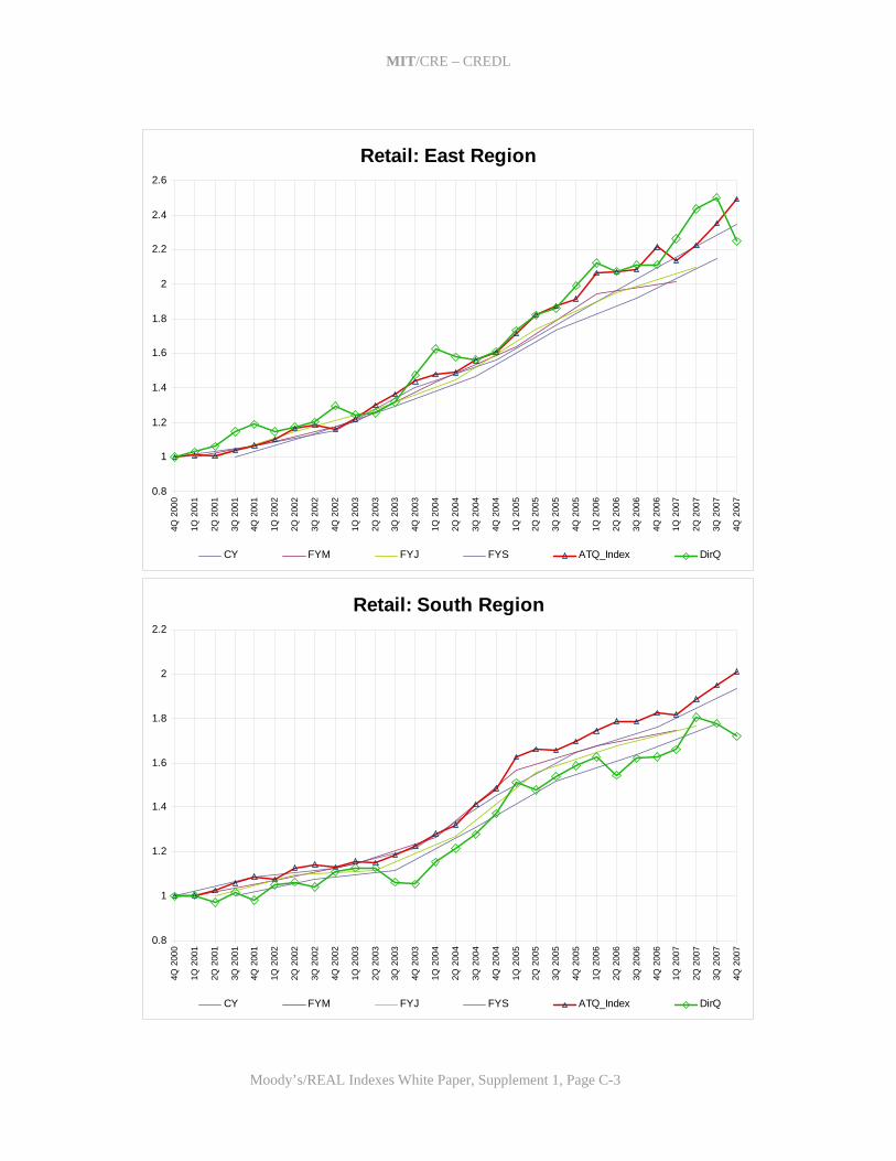
MIT/CRE – CREDL

Retail: East Region

0.8

1

1.2

1.4

1.6

1.8

2

2.2

2.4

2.64Q

200

0

1Q 2

001

2Q 2

001

3Q 2

001

4Q 2

001

1Q 2

002

2Q 2

002

3Q 2

002

4Q 2

002

1Q 2

003

2Q 2

003

3Q 2

003

4Q 2

003

1Q 2

004

2Q 2

004

3Q 2

004

4Q 2

004

1Q 2

005

2Q 2

005

3Q 2

005

4Q 2

005

1Q 2

006

2Q 2

006

3Q 2

006

4Q 2

006

1Q 2

007

2Q 2

007

3Q 2

007

4Q 2

007


Retail: South Region

0.8

1

1.2

1.4

1.6

1.8

2

2.2

4Q 2

000

1Q 2

001

2Q 2

001

3Q 2

001

4Q 2

001

1Q 2

002

2Q 2

002

3Q 2

002

4Q 2

002

1Q 2

003

2Q 2

003

3Q 2

003

4Q 2

003

1Q 2

004

2Q 2

004

3Q 2

004

4Q 2

004

1Q 2

005

2Q 2

005

3Q 2

005

4Q 2

005

1Q 2

006

2Q 2

006

3Q 2

006

4Q 2

006

1Q 2

007

2Q 2

007

3Q 2

007

4Q 2

007



MIT/CRE – CREDL

Apartments: East Region

0.8

1

1.2

1.4

1.6

1.8

2

2.2

2.4

2.64Q

200

0

1Q 2

001

2Q 2

001

3Q 2

001

4Q 2

001

1Q 2

002

2Q 2

002

3Q 2

002

4Q 2

002

1Q 2

003

2Q 2

003

3Q 2

003

4Q 2

003

1Q 2

004

2Q 2

004

3Q 2

004

4Q 2

004

1Q 2

005

2Q 2

005

3Q 2

005

4Q 2

005

1Q 2

006

2Q 2

006

3Q 2

006

4Q 2

006

1Q 2

007

2Q 2

007

3Q 2

007

4Q 2

007


Apartments: South Region

0.8

1

1.2

1.4

1.6

1.8

2

4Q 2

000

1Q 2

001

2Q 2

001

3Q 2

001

4Q 2

001

1Q 2

002

2Q 2

002

3Q 2

002

4Q 2

002

1Q 2

003

2Q 2

003

3Q 2

003

4Q 2

003

1Q 2

004

2Q 2

004

3Q 2

004

4Q 2

004

1Q 2

005

2Q 2

005

3Q 2

005

4Q 2

005

1Q 2

006

2Q 2

006

3Q 2

006

4Q 2

006

1Q 2

007

2Q 2

007

3Q 2

007

4Q 2

007



MIT/CRE – CREDL

New York Metro Office Property Price Index(Based on RCA repeat-sales database as of March 2008)

0.8

1

1.2

1.4

1.6

1.8

2

2.2

2.4

2.6

2.84Q

200

0

1Q 2

001

2Q 2

001

3Q 2

001

4Q 2

001

1Q 2

002

2Q 2

002

3Q 2

002

4Q 2

002

1Q 2

003

2Q 2

003

3Q 2

003

4Q 2

003

1Q 2

004

2Q 2

004

3Q 2

004

4Q 2

004

1Q 2

005

2Q 2

005

3Q 2

005

4Q 2

005

1Q 2

006

2Q 2

006

3Q 2

006

4Q 2

006

1Q 2

007

2Q 2

007

3Q 2

007

4Q 2

007


DC Metro Office Property Price Index(Based on RCA repeat-sales database as of March 2008)

0.8

1

1.2

1.4

1.6

1.8

2

2.2

4Q 2

000

1Q 2

001

2Q 2

001

3Q 2

001

4Q 2

001

1Q 2

002

2Q 2

002

3Q 2

002

4Q 2

002

1Q 2

003

2Q 2

003

3Q 2

003

4Q 2

003

1Q 2

004

2Q 2

004

3Q 2

004

4Q 2

004

1Q 2

005

2Q 2

005

3Q 2

005

4Q 2

005

1Q 2

006

2Q 2

006

3Q 2

006

4Q 2

006

1Q 2

007

2Q 2

007

3Q 2

007

4Q 2

007



MIT/CRE – CREDL

San Francisco Metro Office Property Price Index(Based on RCA repeat-sales database as of March 2008)

0.7

0.8

0.9

1

1.1

1.2

1.3

1.4

1.5

1.64Q

200

0

1Q 2

001

2Q 2

001

3Q 2

001

4Q 2

001

1Q 2

002

2Q 2

002

3Q 2

002

4Q 2

002

1Q 2

003

2Q 2

003

3Q 2

003

4Q 2

003

1Q 2

004

2Q 2

004

3Q 2

004

4Q 2

004

1Q 2

005

2Q 2

005

3Q 2

005

4Q 2

005

1Q 2

006

2Q 2

006

3Q 2

006

4Q 2

006

1Q 2

007

2Q 2

007

3Q 2

007

4Q 2

007


Southern California Office Property Price Index(Based on RCA repeat-sales database as of March 2008)

0.8

1

1.2

1.4

1.6

1.8

2

2.2

4Q 2

000

1Q 2

001

2Q 2

001

3Q 2

001

4Q 2

001

1Q 2

002

2Q 2

002

3Q 2

002

4Q 2

002

1Q 2

003

2Q 2

003

3Q 2

003

4Q 2

003

1Q 2

004

2Q 2

004

3Q 2

004

4Q 2

004

1Q 2

005

2Q 2

005

3Q 2

005

4Q 2

005

1Q 2

006

2Q 2

006

3Q 2

006

4Q 2

006

1Q 2

007

2Q 2

007

3Q 2

007

4Q 2

007



MIT/CRE – CREDL

Southern California Industrial Property Price Index(Based on RCA repeat-sales database as of March 2008)

0.8

1

1.2

1.4

1.6

1.8

2

2.2

2.44Q

200

0

1Q 2

001

2Q 2

001

3Q 2

001

4Q 2

001

1Q 2

002

2Q 2

002

3Q 2

002

4Q 2

002

1Q 2

003

2Q 2

003

3Q 2

003

4Q 2

003

1Q 2

004

2Q 2

004

3Q 2

004

4Q 2

004

1Q 2

005

2Q 2

005

3Q 2

005

4Q 2

005

1Q 2

006

2Q 2

006

3Q 2

006

4Q 2

006

1Q 2

007

2Q 2

007

3Q 2

007

4Q 2

007


Southern California Retail Property Price Index(Based on RCA repeat-sales database as of March 2008)

0.8

1

1.2

1.4

1.6

1.8

2

2.2

2.4

2.6

2.8

4Q 2

000

1Q 2

001

2Q 2

001

3Q 2

001

4Q 2

001

1Q 2

002

2Q 2

002

3Q 2

002

4Q 2

002

1Q 2

003

2Q 2

003

3Q 2

003

4Q 2

003

1Q 2

004

2Q 2

004

3Q 2

004

4Q 2

004

1Q 2

005

2Q 2

005

3Q 2

005

4Q 2

005

1Q 2

006

2Q 2

006

3Q 2

006

4Q 2

006

1Q 2

007

2Q 2

007

3Q 2

007

4Q 2

007



MIT/CRE – CREDL


Southern California Apartment Property Price Index(Based on RCA repeat-sales database as of March 2008)

0.8

1

1.2

1.4

1.6

1.8

2

2.2

2.4

2.6

2.84Q

200

0

1Q 2

001

2Q 2

001

3Q 2

001

4Q 2

001

1Q 2

002

2Q 2

002

3Q 2

002

4Q 2

002

1Q 2

003

2Q 2

003

3Q 2

003

4Q 2

003

1Q 2

004

2Q 2

004

3Q 2

004

4Q 2

004

1Q 2

005

2Q 2

005

3Q 2

005

4Q 2

005

1Q 2

006

2Q 2

006

3Q 2

006

4Q 2

006

1Q 2

007

2Q 2

007

3Q 2

007

4Q 2

007


Southern Florida Apartment Property Price Index(Based on RCA repeat-sales database as of March 2008)

0.8

1

1.2

1.4

1.6

1.8

2

2.2

2.4

2.6

4Q 2

000

1Q 2

001

2Q 2

001

3Q 2

001

4Q 2

001

1Q 2

002

2Q 2

002

3Q 2

002

4Q 2

002

1Q 2

003

2Q 2

003

3Q 2

003

4Q 2

003

1Q 2

004

2Q 2

004

3Q 2

004

4Q 2

004

1Q 2

005

2Q 2

005

3Q 2

005

4Q 2

005

1Q 2

006

2Q 2

006

3Q 2

006

4Q 2

006

1Q 2

007

2Q 2

007

3Q 2

007

4Q 2

007


MIT/CRE – CREDL

Moody’s/REAL Indexes White Paper, Supplement 1, Page R-1

Bibliography Albert, A. (1972). Regression and the Moore-Penrose Pseudoinverse. Academic Press, New York. Aster, R.C, Borchers, B. and Thurber, C. H. (2005). Parameter Estimation and Inverse Problems. Elsevier Academic Press T.Bryan & P.Colwell, “Housing Price Indices”, in C.F.Sirmans (ed.), Research in Real Estate, vol.2. Greenwich, CT: JAI Press, 1982. Chipman, J. (1964). On Least Squares with Insufficient Observations. Journal of the American Statistical Association 59, No. 208, 1078-1111 J.Clapp, “A Semiparametric Method for Estimating Local House Price Indices”, Real Estate Economics 32(1): 127-160, 2004. D.Geltner, N.Miller, J.Clayton, & P.Eichholtz, Commercial Real Estate Analysis & Investments 2nd Edition, South-Western College Publishing Co/Cengage Learning, Cincinnati, 2007. D.Geltner & H.Pollakowski, “A Set of Indexes for Trading Commercial Real Estate Based on the Real Capital Analytics Transaction Prices Database”, MIT Center for Real Estate, Commercial Real Estate Data Laboratory – CREDL, Release 2 (September 26, 2007). Downloadable from: http://web.mit.edu/cre/research/credl/rca.html. D.McMillen & J.Dombrow, “A Flexible Fourier Approach to Repeat Sales Price Indexes”, Real Estate Economics 29(2): 207-225, 2001. Pace, RK & JP LeSage, “Spatial Statistics and Real Estate”, Journal of Real Estate Finance and Economics, 29(2):147-148, 2004. Penrose, R. (1955), “A Generalized Inverse for Matrices”, Proceedings of the Cambridge Philosophical Society 51, 406-413 Penrose, R. (1956), “On best approximate solutions of linear matrix equations”, Proceedings of the Cambridge Philosophical Society 51, 17-19 Schwann, G. (1998), “A Real Estate Price Index for Thin Markets”, Journal of Real Estate Finance & Economics 16(3): 269-287.

http://proquest.umi.com.libproxy.mit.edu/pqdlink?RQT=318&pmid=53480&TS=1206212282&clientId=5482&VInst=PROD&VName=PQD&VType=PQD

http://proquest.umi.com.libproxy.mit.edu/pqdlink?RQT=318&pmid=53480&TS=1206212282&clientId=5482&VInst=PROD&VName=PQD&VType=PQD

a technical note on index methodology enhancement by · pdf fileinclude various types of...

Documents