a technique to calculate complex electromagnetic fields by
TRANSCRIPT

Portland State University Portland State University
PDXScholar PDXScholar
Dissertations and Theses Dissertations and Theses
1978
A technique to calculate complex electromagnetic A technique to calculate complex electromagnetic
fields by using the finite element method fields by using the finite element method
Davood Asgharian Portland State University
Follow this and additional works at: https://pdxscholar.library.pdx.edu/open_access_etds
Part of the Computer Sciences Commons
Let us know how access to this document benefits you.
Recommended Citation Recommended Citation Asgharian, Davood, "A technique to calculate complex electromagnetic fields by using the finite element method" (1978). Dissertations and Theses. Paper 2863. https://doi.org/10.15760/etd.2859
This Thesis is brought to you for free and open access. It has been accepted for inclusion in Dissertations and Theses by an authorized administrator of PDXScholar. Please contact us if we can make this document more accessible: [email protected].

I I
............. --... __ ......... ...._..... ......
AN ABSTRACT OF THE THESIS OF Davood Asgharian for the Master of Science
in Applied Science presented May 16, 1978. ·
Title: A Technique to Calculate Complex Electromagnetic Fields by
Using the Finite Element Method.
APPROVED BY MEMBERS OF THE THESIS COMMITTEE:
James L. Hein
A computer program based on Maxwell's equations is developed to
calculate two-dimensional complex potentials by the Finite Element
Method.· This study offers a solution to a complex continuum problem by
allowing a subdivision into a series of simpl~ interrelated problems.
The region of interest is divided into triangular elements. For each
node in the grid, the Finite Element Method is used to set uy art equa-
tion for the potential as a function of those of the surrounding nodes.
All these equations are solved by the Gaussian Elimination Method. For
increased accuracy this method requires a high degree· of division of the
region of interest. This could cause a storage problem on the computer.
To eleviate this.problem a half-banded scheme is used. A comparison is

! " J
I j-
1·
I I I
-&·-·-------
provided between the data obtained from the developed algorithm and an
actual experiment. In this experiment two-types of sunken swimming
pools, reinforced and non-reinforced, were used to hold three different
waters of conductivities 29µ"V""/cm, 1500µc.r/cm and 3000µ"21"/cm. In order
to test the accuracy of the computer.program developed, the results of
another solved problem are also compared to another computer program's
results which was based on c.apacitive and resistive d·ist:i;:j,bution of
potentials. The result of this study s~ows the hazard may exist on the
edges of the swimming pool when the resistivity of the surrounding soil is high.

i·
1·
I
A TECHNIQUE TO CALCULATE COMPLEX ELECTROMAGNETIC
FIELDS BY USING THE FINITE ELEMENT METHOD
by
DAVOOD ASGHARIAN
A thesis submitted in ·partial fulfillment of the requirements-for the degree of
MASTER OF SCIENCE in
APPLIED SCIENCE
Portland State University
1978

,,
I I· ! I l I
TO THE OFFICE OF GRADUATE STUDIES Al"'ID RESEARCH:
The members of the Committee approve the thesis of Davood
Asgharian presented May 16, 1978.
M. Young, Department ineering and Applied
Graduate Studies and Research
~~
James L. Hein

~.d:IM
f>NIA01 AW O.L
a~.tv~rcraa

ACKNOWLEDGMENTS
The author gratefully acknowledges indebtedness to Dr. V. J. Garg
for his suggestion of the problem, criticisms, and suggestions during
the course of this study and his sacrifice of time and energy during
the writing of this thesis.
The author wishes to express his gratitude to Dr. F. Rad for his
advice and reviewing this thesis. I would also like to express my
appreciation to Professor R. Greiling for making many constructive
conunents.
Consultation with Dr. W. Mueller was also a great aid in the
writing of the computer portion of this study.
The author wishes to thank Ms. Donna Mikulic for the excellent
and efficient typing of this thesis.
I am especially indebted to my dear wife for her encouragement,
understanding and unfailing patience.

TABLE OF CONTENTS
ACKNOWLEDGMENTS
LIST OF TABLES
LIST OF FIGURES
CHAPTER
I INTRODUCTION
1.1 REVIEW OF LITERATURE 1.2 STATEMENT OF THE PROBLEM
II FINITE ELEMENT METHOD
2.1 DEFINITION 2.2 FORMULATION OF FINITE·ELEMENT METHOD 2.3 FORMULATION OF POTENTIAL PROBLEMS WITH SPATIAL
FINITE ELEMENT SUBDIVISIONS 2.4 FINITE ELEMENT SOLUTION OF COMPLEX POTENTIAL
ELECTRIC FIELDS
III COMPUTER PROGRAM
3.1 SOLUTION TECHNIQUE FOR THE FINITE ELEMENT METHOD
3.2 RESULTS OF THE COMPUTER SOLUTION 3.3 COMPARISON OF RESULTS WITH OTHER COMPUTER
TECHNIQUE
IV EXPERIMENTAL PROGRAM
V RESULTS
5.1 COMPARISON OF CALCULATED VALUES WITH EXPERIMENTAL RESULTS
5.2 POTENTIAL HAZARD TO THE HUMAN BODY 5.3 THE LIMITATIONS AND ACCURACY OF THE
THEORETICAL TECHNIQUE
VI CONCLUSION
BIBLIOGRAPHY
Page
iv
vii
viii
1
1 3
4
4 4
8
10
18
18 29
35
38
42
42 52
59
60
61

Page
APPENDIX A EULER'S THEOREM OF VARIATIONAL CALCULUS 63
APPENDIX B THE GAUSSIAN METHOD 66 APPENDIX C CALCULATION OF CURRENT DENSITY 72
APPENDIX D LISTING OF PROGR.A11S AND SUBROUTINES 76
APPENDIX E COMPUTER RESULTS 87
APPENDIX F EXPERIMENTAL RESULTS 100

Table
3.1
5.1 - 5.4
5.5
C.l - C.3
E.l - E.9
E.10 - E.12
F.l - F.9
F.10 - F.12
LIST OF TABLES
Comparison of Results of a Specific Problem
Calculated Current Travelling Through the Human Body Standing on the Soil
Calculated Current Travelling Through the Human Body Inside the Swimming Pool
Calculated Current Densities on the Surface of the Earth
Current Densities Calculated in Soil
Current Densities Calculated in Water
Current Densities Measured in Soil
Current· Densities Measured.in Water
Page
37
54- 57
58
73- ·75
88- 96
97- ·99
101-109
110

Figure
2.1
2.2
2.3
2.4
3.1
3.2
3.3
3.4
3.5
3.6
3.7
3.8
3.9
3.10
4.1
4.2
5.1-5 .. 8
5.9
B
LIST OF FIGURES
Triangular Division of the Area
One Triangle
Typical Triangle with Vertices Marked
Area Coordinates
Region 's' is Divided in 18 Triangular Elements
Banded Form of a Symmetrical Matrix
Flow Chart, Subroutine "BANDWIDTH"
Flow Chart, Subroutine "FIND"
The Finite Element Model
Regional Division of the Experimental Model
Flow Chart, Subroutine "GOOD"
Flow Chart, Program "TES"
Resistive and Complex Admittance Networks
Two Materials in Series
Schematic Diagram of the Experimental Model
Schematic Diagram of the Electrical Circuit
Calculated Current Densities
Levels of Current Hazards to the Human Body
Flow Chart, Subroutine "SOLVE"
Page
5
6
11
11
19
22
24
25
31
32
33
34
35
36
40
41
44-51
53
70

~
CHAPTER I
1-l INTRODUCTION
I 1.1 REVIEW OF LITERATURE
A considerable amount of work has been done in the past in cal-
culating the self and mutual impedance of two parallel ground return
wires. The following paragraphs summarize these attempts in chronolo-
gical order.
The first attempt was made by Carson (1). He investigated the
problem of wave propagation along a transmission system composed of
an overhead wire parallel to the surface of the earth. However a
complete solution of determining the actual impedance is impossible
because of the non-homogeneity of the earth. The solution to the
problem, where the actual earth is replaced by a plane homogeneous
semi-infinite solid has promoted considerable theoretical and prac-
tical interest.
In 1951, Lacey and Wasley (2) at the Hydro-Electro Power Com.mis-
sion of Ontario, Canada, developed an equation for the mutual impedance
of two finite length earth-return circuits, either parallel or at an
angle. The equation developed by them is to· be a generalization of
Carson's work.
In 1965, Wedepohl (3) published a paper on wave propagation in
multiconductor overhead lines which would permit the earth-return path
to have a relative permeability other than unity, which was not permissi-

j.
I I
2
ble in the analysis by Carson. In this paper, the new approach is applied
to the case of a two-layer earth, including the effects of displacement
currents. The results were in agreement with those obtained for the
case of a homogeneous earth.
In 1966, Krakowski (4) developed equations for the mutual im-
pedances of overhead lines with the earth as a return path. In this
paper the problem deals with two different lines which cross each other
at an angle, a., different from zero. A particular case of this pro.bl em
is the same as Carson's solution for a.= 0. The general solution of
this problem is considered, assuming that the earth is uniformly con-
ducting and that both overhead conductors are parallel to the surface
of the earth.
In 1973, Nakagawa (5) published a paper in this area. This
solution permits the earth-return path to be considered as three layers
of different resistivities, permitivities and permeabilities. A strati-
f ied earth causes marked differences in the earth impedances and the
resultant wave deformations from the homogeneous case. The depth of a
layer is a significant factor to the value of the stratified-earth
impedance. The displacement currents can influence earth-return
impedances. This is only at very high frequencies and under the con-
ditions of high earth resistivity and low conductor height.
All these papers prove that there are several ways of calculating
the distributed impedance of ground return transmission lines.
Magnusson (6) developed a method of calculating the mutual and
self-impedance of overhead lines with the earth as a return path. He
also calculated the mutual and self-impedance of the line under the

following conditions:
A. A conductor height of 35 feet
B. A line-to-ground sh~rt-circuit current of 2000 ~mperes.
C. A ground conductivity of 0.01 mho per meter
By the calculated value of the mutual and self-impedance of overhead
lines with the earth as a return path and the use of the developed
formula, he calculated the current densities in a typical below grade
swimming pool.
3
The densities change with respect to the distance of the swimming
pool from the vertical plane of the transmission line. The calculated
current densities in the pool were found to be hazardous to the swimmer
in the swimming pool.
1.2 STATEMENT OF THE PROBLEM
The purpose of this investigation is to develop a computer code
based on Maxwell's equations to calculate potentials between points
of interest on the surface of the earth and swimming pool by knowing
at least two boundary conditions, using the Finite Element Method.
In order to check the validity of this study, the results are
compared to experimental values.
. ,

CHAPTER II
FINITE ELEMENT METHOD
2.1 DEFINITION
The Finite Element Method is a numerical technique for obtaining
approximate solutions to a wide variety of engineering problems. The
ability to use elements of various types and sizes and to model a
system of arbitrary geometry, are the main advantages of the Finite
Element Method.
Other approximate methods, for example the Finite Difference
Method, lacks these advantages. Using these approximate methods, a
specific numerical result may be obtained for a specific problem, but
a general computer solution applicable to all cases is not possible.
The Finite Element Method offers a way to solve a complex con-
tinuum problem by subdividing the continuum into a series of simpler
interrelated problems. It gives a consistent technique for modeling
the system as an assemblage of discrete parts or finite elements.
2.2 FORMULATION OF FINITE ELEMENT METHOD
It is desirable to obtain results in a general form applicable to
any situation. For th.is purpose a division of the region into triangu-
lar shape elements is used as shown in Fig. 2.1.
The problem is to calculate the values of ~e) (i.e., voltage)
(e) at each node, (N = 1, 2, ••. , n) by knowing values of RN at some node

5
y
5 4
3
2
x
Figure 2.1 Triangular division of the area.
as boundary conditions.
The integer numbers of 1, 2, ••• , n represent the number of the
particular node and value of H at node 5 which is written as H5
• The
integer numbers written inside parenthesis, for example, (3) represents
the element's number.
Each element has three nodes and each node has its own coordinate
values. For example, element (1) has nodes 1,2,7 and coordinate·
values of (x1
, y1), (x2' y 2)' (x7 , .Y7), and element (5) has nodes 6,7,5
and coordinate values of (x6
, y6),
(x:Y-j Y7)' (x5, Y5). Fig. 2.2 shows a typical triangie from the whole area of Fig. 2.1.
The assumption is that the value of h (i.e., voltage) at any point
inside the triangle is a linear function of Hat the triangle's three
nodes, or simply:

6
HR. h(e) = [N(e) N(e) N(e)] I Hm f ~ [NJ[H] 2-1 R. m m
H m ...
yl R,
m
n
x
Figure 2.2 One triangle element.
Therefore, for the area of Fig. 2.1, the values of h in each
element are:
h(l) = N(l) H + N(l) H + N(l) H 1 1 2 2 7 7 2-2
h(Z) = N(2) H + N(Z) H + N(2) H 2 2 3 3 7 7 2-3
h(J) =·N(J) H + N(J) H + N(J) H 3 3 4 4 7 7 2-4
h(4) = N(4) H + N(4) H + N(4) H 4 4 5 5 ] 7 2-5
h(S) = N(S) H + N(S) H + N(S) H 5 5 6 6 7 7 2-6
h(6) = N(6) H + N(6) H. + N(6) H . 6 6 1 1 7 7 2-7
Where [NJ is called a shape function and will be seen later to
play a paramount role in the Finite Element Method. The shape function
is a function of area coordinates:

7
N(e)= l/2A (e) fa (e)° + b (e) X + c (e) Y] n n n n 2-8
Where A = area of the triangle:
a = x y - x y· n .Q, m m R..
b = y - y n .Q, m
c = x - x n m R..
For example N7
for element (4) is:
N(4) = l/2A(4) [a(4) + b(4) X + c(4) Y] 7 7 7 7
Where: a7 = X4Y5 - x5Y4
b7 = Y4 - Y5
C7 = XS - X4
and so on.
The total h in this area is equal to the summation of hS in the
elements.
E h(e) h=L 2-9
e=l
Where E is the number of the last node. Eq. 2-9 could be written in
matrix form as well as in summation form.
h(l) N(l) 1
N(l) 2
0 0 0 0 N(l) 7 Hl
h(2) 0 N(2) N(2) 0 0 0 N(2) H2 2 3 7
h (3) 0 0 N(3) N(3) 0 0 N(3) H3 I 2-10 = 3 4 7 h(4) 0 0 0 N(4) N(4) 0 N(4)
H4 4 5 7 h(5) 0 0 0 0 N(5) N(5) N(5)
HS 5 6 7 h(6) N(6) 0 0 0 0 N(6) Nj6)1 I H6 1 6

2.3 FORMULATION OF POTENTIAL PROBLEMS WITH SPATIAL FINITE ELEMENT SUBDIVISIONS
8
The current density JT consists of both conduction and displace-
ment components, respectively:
JT = CTE + (d/dt)D 2-11
where
D = jtWEE 2-12
After subseitution of Eq. 2-12 into Eq. 2-11 one may obtain this result:
JT = (cr + jwE)E
Equation 2-13 by Kirchoff's law must satisfy the continuity
equation.
or
but
where
v • J = 0 T
V • (a + jwE)E = 0
E = -VV = 0
v . (cr + jwE)VV = 0
vv = [(a/ax)Va + (a/ay)Va + (a/az)Va ] x y z
Substitute Eq. 2-18 back in Eq. 2-16:
2-13
2-14
2-15
2-16
2-17
2-18
v • (cr + jwE)[(a/ax)Va + (a/ay)Va + (a/az)Va] = o 2-19 x y z
v · A= (a/ax)A.+ Ca/ay)A + Ca/az)A 2-20
Therefore the resultant equation is:
(a/ax)(cr + jwE)(a/ax)V + (a/ay)(cr + jwE)(a/ay)V +
(a/az)(cr + jwE)(a/az)V = o 2-21

In order to solve Eq. 2-21 one may need to know Euler's theorem of
variational calculus, as outlined in Appendix A. By the help of
variational calculus, a function I(V) could be found where oI(V) = 0
everywhere.
( 2 , 2 I(V) = l/2Jn [(a+ jwg)(av/ax) +(a+ jwE)(av/ay) +
2 (a + jwE).(aV/az) ]dx dy dz
but 3
v(e) = .L.: N v = [N] [V] (e) i=l i i
The derivative of I(V) with respect to the Vi is equal to z.ero.
ar(v)(e) /av.= o i
=J0
{r<cr + jwe)(av<e>/ax)(a/av1)(av<e>/ax)J +
[(a+ jwE)(av<e)/ay)(a/avi) av(e) /ay)] +
9
2-22
2-23
[(a+ jwg)(av(e)/az)(a/avi)(av(e)/az)l} dx dy dz 2-24
But from Eq. 2-23 it is obvious that the derivative of V(~) with respect
to x is: 3
av(e)/ax =~ (aNi/ax)Vi = [aN/ax][V](e) i=l
2-25
(a/avi)(av<e)/ax) = (a/avi)[(aN1 /ax)Vi1 = aN1/ax 2-26
where
av(e)/avi =Ni 2-27
The result of the substitution of Eq. 2-25, 2-26 and 2-27 back in Eq.
2-24 is:

ar(v) (e) /avi = o = LJca + jwe:)[aN/axJ[vJ (aNi/ax) +
(a+ jwE)[aN/ay][V](aN./ay) + 1
10
(cr + jwE) [aN/az] [V] [aN/az] }ax dy dz 2-28
Where:
Equation 2-28 could be written in general form as:
[K][V] = [O]
K. . = ( ((a + jwE) (aNi/ax) (aN ./ax) + (cr + jwE) (aNi/ay) i,J Jnl' J
(aNj/ay) + (cr + jwE)(aNi/az)(aNj/az)} dx dy dz
2.4 FINITE ELEMENT SOLUTION OF COMPLEX POTENTIAL ELECTRIC FIELDS
The region of the problem can be subdivided into triangles in
2-29
2-30
any desired manner, insuring only that all different material interfaces
coincide with triangle sides. Figure 2.3 shows a typical region divided
into triangles.
It is assumed that there is a linear variation of potential within
each triangular element with respect to the nodal potentials.
A convenient set of coordinates 11
,12
,13
for a triangle 2,m,n,
Fig. 2.4, is defined by the following linear relation between these and
the Cartesian system:

y
( k: "In
'( \ ~m
Figure 2.3 Typical triangle with vertices marked.
\ \
\ \
(xn,yn)
\ \ \ \ ..
x
L1=1 ~ \ \PCL1 ,L2 ,L3)\ ~ .!l . \ \. \ m
~ ' < ,~,( (x.!l,y.!l) ' \ ' ' xm,ym)
Figure 2.4 Area coordinates.
11

12
x = 11xi + 1 2xm + 1 3xn
y = 11Y~ .~ 12Ym + 13yn
1 = 11 + 12 + 13 '
To every set, 11
, 1 2 , 13
(which are not independent, but are
related by the third equation) corresponds a unique set of Cartesian
coordinates. At point 1, 1 1 = 1 and 1 2 = 1 3 = O, etc. A linear re
lation between the area coordinates and Cartesian coordinates implies
2-31
2-32
2-33
that contours of 11
are equally placed straight lines parallel to side
2-3 on which 11
= 0 etc. It is easy to see that ~n alternative defini
tion of the coordinate 11
of a point P is by a ratio of the area of the
shaded triangle to that of the total triangle.
1 = area Pmn 1 area R-mn
One may write Equations 2-31 through 2-33 in matrix form and solve it
for 11 , 1 2 , 13
.
xi
y R,
1
x m
ym
1
x n
yn
1
11
12
13
x
= y
1
2-34

l l l
UA UIA ?5 t\
8£-Z u Ul ox x x vz £1 ?5 Ul Ul 0
( ?5 AUIX -UIA ?5 X) ( x -x)a + ( a -a)x + 1 1 1
.6. UIA 0.6.
Ul ?5 x x x
l l l
UA UIA o.6.
u Ul ox l£-Z x x vz
z1 u ?5 0 u (UA?fX -oAUX) = = ( x -x).6. + ( .6. -.6.)x + l l l
UA .6. 0 £.
u 0 x x x
l l l
u.6. UIA oa
9£-Z u Ul ?5 x x x vz = 11
(Ul.6.Ux -·UaUIX) = Ul ux).6. + (u£. Ul ( x --.t\)x + .T 1 1
UA UIA ..:\
u Ul x x x
£1

14
Where:
2A = 2*(area of the triangle) = (x y - x y ) + (x Yn - XnY ) + mn nm nx, x,,m
(xRXm - xm Y2) 2-39
The area coordinates are the shape functions: N1
= L1
,N2
= L2
and
N3 = L3.
The potential inside the triangular element is a linear function
of the nodal's potentials:
v(e) = L V + L V + L V 1 R, 2 m 3 n 2-40
After substituting Equations 2-36, 2-37 and 2-38 into Equation 2-40
one obtains:
v(e) = l/2A [[(x y - x y) + x(y - y) + y(x - x )]Vn + mn nm m n n m x,,
[(x y - x y ) + x(y - y ) + y(x - x )]V + ni in n R, R, nm
[(x y - x y ) + x(y - y ) + y(x - x )]V ] R,m mi R, m m R, n 2-41
In order to solve Equation 2-28 the .shape functions must be known.
When they are determined they can be substituted in Equation 2-42.
[K] [V] = [O] . 2-42
Matrix K is calculated for a two dimensional problem.
Kij = J [(cr + jwE)(aNi/ax)(aNj/ax) + '(cr + jwE)(aNi/ay) n
(aN./ay)] dx dy 2-43 J

"l
15
For each element (a + j WE) may be taken outside the integration sign.
Therefore:
2 2 Kl,l = [(dN1/dx) + (dN1/dy) ]dx dy
(x -x ) 2 ( 2 2 n m Y -y ) + (x -x ) + 2 ] dx dy = m n n m
4*A 4*A 2-44
Kl,2 (y -y )(y -yn) (x -x )(xn-x)
= [ m n n x.. + n m x.. m ]dx dy = 4*A2 4*A2
(y -y )(y -yn) + (x -x )(xn-x) m n n x.. nm x.. n 4*A 2-45
Kl,3 (y -y )(yfl-y) + (x -x )(x -xn) mn m nmmx..
4*A 2-46
K2,l = Kl,2 2-47
2 2 (y n -y Jl) + (x Jl -xn)
K2,2 = 4*A 2-48
K2,3 (yn-yJl)(yJl-ym) (xJl-xn)(xm-xJl)
= [ + ]dx dy = 4*A2 4*A2
(y -y )(y -y) + (x -x )(x -x) n Jl Jl m Jl n m 2
4*A 2-49
K3 1 = Kl 3 ' '
2-50

16
K3,2 = K2,3 2-51
K3,3
2 2 (yi-ym) + (xm-xi)
4*A 2-52
Substituting Equations 2-44 thru 2-51 into Equation 2-42 and writing the
result in matrix form:

2 (y
m-y
n)
(yn
-y i)
+
(y
-y
)
+
m
n 2
(x -x
)
(x -x
)
(xi -
x
) n
m
n m
n
(ym
-yn
)(y
n-y
i) +
2
P/4*
A*
I (y
n-y
i)
+
(x -x
)
(x2-x
)
2 (x
2-x
n)
n m
n
(Y
-Y
)(Y
2-Y
) +
m
n
m
(Yn
-Y 2
) (Y
2-Ym
) +
(X
-X
) (X
-X
i)
n m
m
(X
2-Xn
) (X
m -X
i)
(y m
-y n)
(y i -y
m)
+
I I
v (x
-x
)
(x -x
i)
i n
m
m
(yn
-y g_}
(y
i-y
m)
+
I I
v (x
2-xn
) (x
m -x
2)
m
(Y R
,-Ym
)2 +
I I
v (X
m-X
R,)
2 n
I I
I =
I
I I
0 0 0
I 2-
53 1-
4 -...
.J

CHAPTER III
COMPUTER PROGRAM
3.1 SOLUTION TECHNIQUE FOR THE FINITE ELEMENT METHOD
A computer program is written to.solve Eq. 2-53 f~r the region of
interest which consists of n-type of materials and at least two boundary
conditions. This equation in the short form is given by:
[K] [V] = [O] 3-1
Matrix [K] is the coefficient matrix and consists of all the pro
perties of the materials in the region. Each element in the region
could have a different property from the others. Matrix [K] is calcu
lated for each element with its own properties and then transferred to
the final coefficient matrix [F]. One example is given below.
Region S, Fig. 3.1, is divided into 18 triangular elements and
each element has been numbered from 1 to 18.
Also all nodes are numbered in a fashion to create a sparse [F]
matrix to reduce the band-width of the [F] matrix. To do so, the side
which has less nodes than the other is determined. Then the nodes are
numbered from one end to the other and returned to the original side,
as shown in Fig. 3.1. This method insures the smallest possible band
width for the [F] matrix.

19
y
13 14 15 16
9 L -,....c: =-tc ., 12
5 • Naz ==:.: ., 8
l• JM 3>' < - 4 2 j
x Figure 3.1 Region S is divided in 18 triangular elements.

20
The arbitrary element Z has nodes 2,m,n and coordinates of (xN
YN ), (xNm, YNm), (xNn, YN~) and material property of P. By using
Eq. 2-53 we can solve for matrix K:
KR,' R. K Jl,m K
R. ,n
K = I Km,R. K K m,m m,n 3-2
K K K n, R. n,m n,n
By transformation, Kt Jl goes to the [F] matrix in row Jl and column '
Jl and then added to the previous value of F2 , 2• Similarly, KR.,m goes
into the row Jl and column m of the matrix [F] and then added to the pre-
vious values of F0 , and so on. N,m
After completing the matrix [F], Equation 3-1 becomes:
[F][V] = [O] 3-3
where it has the dimension of (No. of nodes by No. of nodes) and K is
a 3 by 3 matrix. Since Equation 3-3 is equal to zero, it requires
the boundary conditions for solution. The boundary conditions are used
to create values on the other side of the equation.
For instance, region S in Fig. 3.1 has two boundaries, one at each
end. Nodes 1,5,9 and 13 from one end and nodes 4,8,12 and 16 from the
. . other end are the boundary nodals and have known values of voltage •
Therefore we can leave these nodes out of our calculations. For example:
element (7) has nodes 5,6,9 where nodes 5,9 have known values and node 6
is an unknown.
The matrix notation for this element after calculating the K
matrix is:

21
0
=
~,5 K5,6
K6,5 K6,6
KS,9
K6,9
K9,9
vs
v6
v9
0
0
3-4
K9,5 K9,6
Therefore there is just one equation and one unknown and it is
easy to transfer the known values to the other side of the equation.
The result is:
[K6,6][V6] = [-K6,5 *VS - K6,9 * V9] = [B6]
Now this equation is transferred to the [F] matrix:
[F][V] = [B]
For the small size of matrix [F] we can find the inverse of the
[F] matrix and multiply it with the [B] matrix to find the values of
the nodes.
3-5
3-6
All finite element solutions require a high subdivision of the
region for the utmost accuracy. This makes matrix [F] so large that it
becomes useless to solve by the invertion of the [F] matrix.
Due to the nature of the problem, provided that the nodes are
numbered in a careful manner, the non-zero terms in matrix [F] will be
concentrated in a narrow band situated adjacent to the leading diagonal.
This fact, combined with the symmetrical nature of matrix [F] indicates
that only a relatively small portion of the matrix is of real interest.
If advantage is taken of these observations, demands on the computer
storage may be considerably reduced. Moreover, if the solution procedure
is so arranged that many of the operations involving the zero terms are
eliminated, the speed of the solution can be increased. Methods which

22
take advantage of the banded nature of matrix [F] are often called
'banded methods'.
Methods which off er potentially greater economies are the so-called
'half-banded schemes'. The upper half of the diagonal band of the matrix
is stored as a rectangular matrix as shown in Figure 3.2.
._B_.
r SIZE
+--" B--+
UPPER HALF BAND
" "
,,~ ,, 1c"'" ZERO
MATRIX F MATRIX A
Figure 3.2 Banded form of a synnnetrical matrix.
The upper half band part of matrix IF] is stored in matrix {A]
which is much smaller than matrix (F]. Matrix [A] has a number of columns
equal to the bandwidth and rows equal to the number of nodes. Each row
of matrix [F] is transferred to matrix [A].
To calculate the band-width of a finite element problem, one must
know the number of all elements and their node numbers, because bandwidth
is equal to the largest difference between two nodes in one element;
that is compared to the rest of elements + 1.
Figure 3.3 is a flow chart of the computer program which finds the
bandwidth of matrix [F] or any other symmetrical matrix. Figure 3.4
is a flow chart which determines the coefficient matrix and transfers
the upper half part of matrix [F] to matrix [AJ.
Equation 3-6 takes the form:

23
[A]fVJ = fB]
It is impossible to find the inverse of [A] because it is no longer a
square matrix. Theref~re, the Gaussian Elimination Technique is used
3-7
to solve Equation 3-7. Another step to save memory space is to eliminate
matrix [V] from the equation. To do so, the problem between [A] and
[B] is solved and the result is stored in matrix [B]. Mat~ix [B] has
the same dimension as matrix [V].
For more understanding of the Gaussian Elimination Technique an
example is solved in Appendix B along with the flow chart.
Appendix D includes a listing of the main program as well as all
subroutines discussed in this chapter.

YES
NO
SET ~ANDWIDTH•O
K = 1
READ NOD.ES AND LAST NODE BEFORE BOUNDARY NODE
CALCULATE THE (DIFFERENCES BETWEEN EACH TWO NODES) + 1
FIND THE LARGEST LET IT BE Bwl
BANDWIDTH = Bl
RETURN
NO K = K+l
Figure 3. 3 Flow chart, subrout_ine "BANDWIDTH".
24

25
START
M-1, NUMBIB OF NODES IN F.ACH ELEMENT
I•1, NUMBER OF NODES IN EACH ELEMENT
YES
YES
NO
MM • N(M) MM• N(M)
I.CULATE A(MM,1) CALCULATE A(MM,1) CALCULATE A(MM,1) ..
Figure 3.4 Flow chart, subroutine "FIND".

NO
YES
NO
NO
CALCUUTE B(~'N)
WHERB h1l = N(M)
Figure 3.4 (Continued)
YES
MM = N(I)-N(M) + l
NN = N(M)
CALCULATE A(NN,MM)
26

f YES
NO
NO
CALCULATE B(NN)
WHERE NN = N(M)
y.r;s
HM • N(I)-N(M) + l NN -= N(M)
CALCULATE A(NN,MM)
Figure 3.4 (Continued)
27

CALCULATE B(~N)
WHERE NN ::: N(M)
NO
NEXT I
NEXT H
RETURN
Y~S
MM • N(I)-.S(M) + l
NN • N(M)
CALCULAT£ A(:.'iN,MM)
Figure 3.4 (Continued)
28

29
3.2 RESULTS OF THE COMPUTER SOLUTION
The problem was to calculate current densities everywhere in the
region S. Region S was a large area of soil with a sunken swimming pool
in the center of the region. The region was divided into 76p ~lements
with three types of materials and two boundary conditions. Figure 3·.5
shows the subdivided region of 'S'.
For large problems such as this involving many elements, it is
useful to possess a routine which generates the complete set of data for
the finite element program.
Region 'S' was subdivided into five regions. Region one was below
the swinnning pool, region two and four were the swimming pool ends and
the soil; region three was the swimming pool and surrounding soil; and
region five was above the swimming pool. Figure 3.6 shows these five
regions.
The reason for dividing regi~n 'S' into five regions was to make
data preparation easier. Regions 2,3,4 were divided in a different
fashion than 1 and 5. Region 1,5 and 2,4 are identical in values of x
and y with some constant. Also the results of each region can be stored
in a different matrix and recalled when needed. All nodes on each
boundary are given the same number for simplification purposes.
A subroutine was written to find the coordinates of all nodes.
Figure 3.7 shows a flow chart of such a subroutine.
Figure 3.5 shows that nodes 1,10,19,28 and 37 have the same value
of x and nodes 1,2,3,4,5,6,7,8 and 9 have the same values of y. Therefore
coordinates of nodes are calculated and stored in a matrix for later use.

30
Another data file is generated which consists· of all elements with
their nodal numbers. Figure 3.8 shows .a flow chart ot this program
(called "TES") which can read the element's number and their nodal numbers
from the file and find the corresponding coordinate values and store them I
in a separate file, which ~acks the information about the first and last
row of the.region 'S'. This information could be added to the file
easily.
This data file is ready to be given to the main program for cal-
culation of voltages at each node. A program is written to calculate
the current densities in the region in the y-direction.· Results of
computer program, in tabular form are given in Appendix E.
A comparison of the computer results with experimental results is
given in Chapter V.

1£

32
R E G I 0 N 0 N E
L- - - -- - - - - - - - - - - - ... - - - - - ..... - - - - - --
R £,G I 0 N T W 0 L - - - - - - - - - - - - - - - - - - • - -t - - - - - - - - - - - - - - - ":- •
l
R 1': G l 0 N T H RIE ~
l---------------1--. __ .,. ______ ,_ ________ _ R E G I 0 N F 0 U IR
L... - - - - - - - - - - - - - - - - - - - - - - - - - - - - - - - -a...~
y
R £ G I 0 N F I VE
x
Figure 3.6 Regional division of the experimental model.

START
READ ALL X, Y
LE'T NODES OF AREA BE REPRESENTED BY A 11.ATRIX
I = l,N J = l,M
A(I,J) = K+J
YA(I,J) = Y(I)
K = K+M
NEXT J,I
CALCULATE THE X-COORDINATE
I = l,N J = l,M
XA(J,I) :: X(I)
NEXT J ,I
REnJRN
Figure 3. 7 · Flow chart, subroutine "GOOD".
33

START
READ X(I), Y(I) FROM Sl'OOAGE
RF.AD NUMBER OF ELEMENT,
rrs. NODES AND PROPESTY
L • NODE 1 J •NODE 2 K •NODE 3
XN(1) • X(L), YN(1) • Y(L) XN(2) • X(J), YN(2) • Y(J).
XN(3) • X(K}, YN(3) • Y(K)
READ IN DATA FOR ARE.A 2,4 <F THE REnION'S'
STOP
NO
Fi~ure· 3.8 Flow chart, program "TES".
34

35
3.3 COMPARISON OF RESULTS WITH OTHER COMPUTER TECHNIQUES
In order to check the accuracy of the proposed theoretical technique
which is based on Maxwell's equations, solutions to selected problems were
compared to results obtained using another computer program, which calcu-
lates electric fields in configurations with both capacitive and resis-
tive distribution of potentials (Anderson, 1976, Ref. No. 16).
5 5
4 4
1
3 ·3
Figure 3.9 Resistive and complex admittance networks.
Figure 3.9 shows triangular elements and their complex admittance
network. The resultant equation for the complex potential at the center
node is:
v 0
= 1
6 LCG+jB)n n=l
6 ~ (G+jB). V L__ n n
3.8
n=l
To check the accuracy of the program, results of a specific problem
are compared.

36
A square of 100 x 100 mm is divided up into two series connected
halves, one where the capacitive distribution dominates, and one where
the resistive distribution dominates. Permittivities and conductivities
are chosen in such a way that the voltage across each half has the same
magnitude (Fig. 3.10). A very coarse subdivision of only 16 triangular
elements is used.
v = 100 y
v = 0
I e: = 100 y = 0 f = 50 Hz e: = 0.01 _1_ y = 278.031
GOm
Figure 3.10 Two materials in series.
Table 3.1 shows the comparison of results using Andersen's solution
and the proposed solution, to the actual values. As evident from Table
3.1, agreement between the proposed solution and the actual values is very
close.

, I
37
TABLE 3.1
Sta. Actual Values Andersen's Proposed Solution . Solution
y lOO+jO lOo+jO lOO+jO
c 75+j25 74.99+j24.97 74.9999+j24.9695
B 5o+j50 4 9 • 98+j 50. 02 49.9999+j50.0001
A 25+j25 24.99+j24.99 24.9999+j24.9999
x O+jO O+jO o+jO
Also, the accuracy of the proposed theoretical solution was veri-
f ied by comparing the results of the theoretical solution to known actual
values. In all cases very close agreement was observed.

CHAPTER IV
EXPERIMENTAL PROGRAM
In conjunction with the theoretical analysis, an experimental
program was set up. This experiment was based on an average current
density of 0.07 amp per square meter in the uniform ground under the
transmission line. (See Appendix C.)
In order to create a similar situation for the experiment, a large
box with conductors at two ends was chosen to hold the soil and the
swimming pool. Figure 4.1 shows a schematic diagram of the box.
To create a uniform current density throughout the soil a known
voltage calculated from Equation 4-1 was applied across the conductors.
J • Ea = E/p
where . J = current density
p = resistivity of soil
a = conductivity of soil
E = applied voltage
Resistivity of the soil was calculated from Equation 4-2.
R = V/I = pf/s a t/as
4-1
4-2
The experiment was done for three different resistivity values for
the soil, each soil type with two different types of swimming pools,
reinforced and non-reinforced swimming pool; and each swimming pool

39
containing three different types of water.
Three· resistivity values for soil and conductivity values for water
were:
For Soil For Water
a: 1000 ohm-meter 30 micro-mho/cm
b: 55 ohm-meter 1500· micro-mho/cm
c: 10 ohm-meter 3000 micro-mho/cm
To determine the current densities, first potentials at predeter-
mined points were measured and then current densities were calculated
from potential measurements.
current densities _ difference in two potentials - {distance between two potentials)* conductivity of
the material
Figure 4.2 shows a schematic diagram of the circuit used to measure the
potentials at each point.
Reference 18 contains a detailed description of the experimental
program and results. Selected results of this experimental program are
presented in tabula~ form in Appendix F.

, I
4•
Conductor
/. .,?soil_
-•k-/ ~ soil
'--
9' ~ Transverse Cross Section
1.-3.61~ l. •
40
Conductor
3.51
I-< 14.4' · .1 Longitudinal Cross Section
Figure 4.1 Schematic diagram of the experimental model.

, 1
~1 ~~~ ' __ 1 IW
J1 ' CO~Dt:CTOR l
}I r , 7
PROSE 2 --SWIMMUIG POOL
PROBE 1 --.
CO.\u'i,;CTO~ 2
'
l lj~ _ 2 -
I SWITCH
I DIGITAL M£TER l
0 -' I
0 + T I
SWITCH 1 TO MEASURE VOLTAGES IN THE SOIL. SWITCH 2 -TO MEASURE VOLTAG~S IN THE WAT£.~.
Figure 4.2 Schematic diagram of ·the electrical circuit.
41

CHAPTER V
RESULTS
5.1 COMPARISON OF CALCULATED VALU~S WITH EXPERIMENTAL RESULTS
In order to compare the calculated results with the measured
values, current densities of medium case (resistivity of the soil = 55
ohm-meter) are plotted in Figures 5.1 to 5.8.
In these figures, current densities are plotted versus distance.
Each figure represents calculated and measured current densities in
the soil as well as the swinnning pool.
The calculated current densities in these figures show the expected
synnnetry of the system about the center line, Figures 5.1-5.8. This is
one verification of the accuracy of the computer program.
The measured values of current densities do not show the same
exact synnnetry. This could be explai~ed in terms of the accuracy of the
instruments. Also the conductivity of the soil is not uniform everywhere
and the given value of conductivity is only an average measured value.
Another reason for the discrepancy between the theoretical and measured
values is the two dimensional computer modeling, which assumes the
swimming pool walls to be infinitely long in the z-direction (depth).
The calculated values of the current densities between stations
1 to 6 and 12 to 17, Figures 5.1-5.2, in the soil are higher than
measured values. The measured values of current densities inside and
outside the swimming pool between stations 6 to 12 are higher than

43
calculated values. Between stations 6 to 12 the theoretical model
assumes a plate of iron bars of infinite depth. Due to this plate of
high conductivity, the potential gradients along the plate are zero,
resulting in zero current densities along the line 'C'. Furthermore,
the current flowing along the paths 'A' and 'B' are attracted toward the
infinite iron plate resulting in lower values of current densities along
'A' and 'B' as compared· to the experimental case, where only finite
plates of iron bars exist.
Along the line 'D', the calculated current densities must-go through
the infinite iron plate, while in the measured case the current paths
go through the bottom surface bars of the swimming pool. Results in
tabular form are shown in Appendices D and E.
The reason for higher current densities and potential gradients
along the line 'C' between stations 6-8 and 10-12 is the sharp change in
material conductivities at these stations (soil conductivity = 1.8 x 10-l
mho/m; iron conductivity 1.1 x 10⁶ mhofm). Due to high conductivity
of iron bars the current is attracted toward the pool walls and thus
increasing the field (potential gradien~) around the corners.
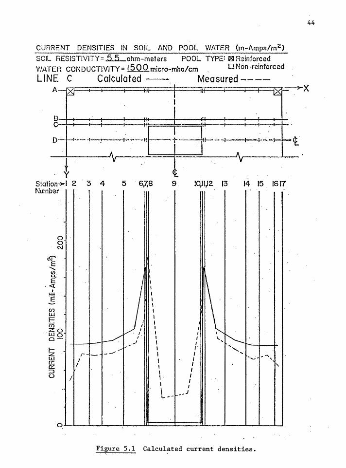
CURRENT DENSITIES IN SOIL AND POOL WATER (m-Amps/m2 )
SOIL RESISTIVITY= 5 5 ohm-meters POOL TYPE= 181 Reinforced WATER CONDUCT1VJTY= 1500.micro-mho/cm . DMon-rainforced
LINE C Calculated Measured----A
8 c ; ~-~-:---:-=--~r -t f 1 D -J I I- J I
t Station~I 2 Numbar
~
.0 o· C\1
(\J .
E ....... (/)
n -E
. <(
• .!. ·e ~
(j)
~ 1 <n zo ·wo c-
lz w er. ~ . (.) I
I I
~
3 4 5
r-1-..1- __./
. E?,7,8
~ I I
' ' ' ' ' '
9. 10,11,12
' ' , t I I I l I l I I' l I \ I I I \ I \ . I \ I \ I l- .. - __ J
13· 14 15 1617
\~ \.. . ... ' .
' ..... ... _.oi-"'°',
'I '\
o..-._,_ __ .._~--~----...-1~--~--~----""-'-----"~~----.____,.._,
Figure 5.1 Calculated current densities.
44
t-.

l
I 45
CURRENT DENSITIES IN SOIL AND POOL WATER (rn-Amps/m2 )
SOIL RESISTIVITY= 5 5 ohm-meters POOL TYPE= ~Reinforced WATER CONDUCTIVITY:: 15 00 micro-mho/cm . DMon-reinforced
1 ·LINE D Calculated Measured----A
8 c
D
.f y
Station~I 2 Number
.
0 o· C\J
<§"' • E
' (/).
0. -E
. <( . .!. .E -CJ) w -l-m zo wo· o-
-r
3
Jz w 0:::: I _, _ _... 0:: :::> • (.)
I ,_
4 5
''I • -----x •• l 1 "'/.~,-
"I I
I" + -1 I I- t·I h
6;7,8 9. 10,11,12. 13' 14 15 1617
I I
I I
I··
.,... ____ ..... _____ .
'1\ I \ ~ \
' ' ' - ......... ,
"'
Q.J.._.J......--.L--1-~~..L----LlU===========::W--~.J---......L---l-~.J.....I
Figure 5.2 Calculated current densities.

l
I
I CURRENT DENSITIES IN SOIL AND POOL WATER (m-Amps/m2 )
SOIL RESISTIVITY= 5 5 ohm-meters POOL TYPE: ~Reinforced WATER CONDUCTIVITY=30QO micro-mho/cm DNon-reinforced
LINE C Calculated Measured----
AT ll I Ill ! HI : : : r-x 8 ' i I I 1:1 I "Ii '
~ ~ II I - ::1 t 1:: - : : : - : i t i JI. . A.
y <t Station~ I 2 3 4 5 6;7,8 9 IO,fl>l2 13 14 15 1617 Number
t<J' E
........ (f)
a.. E <! • ..!. . E
en w t-
0 0 C\J
(f)
zo wo o-
rz w 0::: 0::: :::> (.)
0
-
.
.
.
.
-.---
. r
I I
I I
.
.
h .. \
\ \
\ \ \ . \ \ \ \ \ \ \
' \
' \ \ I '
__./" I ,.
I "'--- ,/ \ I \ - r--. -: ,, \ I " - ... ., . \ ........ ' """"" ..... _,,,,
I -~· \ \
I ~
\ \ I
' . ' I \ .... -' i...-
Figure 5.3 Calculated current densities.
46

l
!
CURRENT DENSITIES 1N SOIL AND POOL WATER (m-Amps/m2 )
SOJL RESISTIVITY= 5 5 ohm-meters POOL TYPE= ~Reinforced WATER CONDUCTIVITY= 3Q00micro-mho/cm DMon-reinforced
LINE D Calculated Measured ----A ---~~~--~~~~~~------~~--~...,.__,__ ______ ~x
8 l •
c 1 i J ) i li' I
D I ' I I '
.. t . y
Station~ I 2 3 4 Number
~ E
.......
0 o· N
CJ)
~ E .. . <(
• .!. .E .
(/) w t-oo zo
. l.1.1 0 c-l-z ,,,..... w ,.. 0:: 0:: => (.)
5 ~;r,a 9. lqfl)2 13
11------1-- - - -
t-- l I <t··
14 15 1617 ..
'
Q I I I I I Ill I IJI I l I I I
Figure 5.4 Calculated current densities.
47

CURRENT DENSITIES IN SOIL AND POOL WATER (m-Amp:>/m2 )
SOJL RESISTIVITY= 59.5 ohm-meh~rs POOL TYPE: 0 Reinforced WATER CONDUCTJVITY = 16 OQ_micro-mho/cm . rzl Non-rainforced
LINE C Calculated Measured -- --A
~ y Station-:-- I 2 3 Number
-
o_ 0 C\J
c:\J E
........ CJ).
a.; . -E
. <( • ..!.. .E --CJ) w -I-en zo WQ o-I- -z w er: 0:: :::> (..)
0
r--
4 5
.
Ill
. 6,7,8
\ \ \ \
t 9.
I
;:1 l l 1 ,V!-~x
..
r 10,11,12
'Ill I I I I I I I
-1 I J·- i t-t.
13 14 15 1617
F·igure 5. 5 Calculated current densities.
48

, i I
CURRENT DENSITIES IN SOIL AND POOL WATER (m-Amps/m2 )
SOtL RESISTIVITY =59.5 ohm-meters POOL TYPE= D Reinforced
WATER CONDUGT!VITY =1600 micro-mho/cm . r2I Non-reinforced
LINE D Calculated Measured----
AT I : : ::: I l:: : : : r-x ~: ' .. , l !·· .
D I I • A - "I i 1:, - I ~' =ft t
Station~ I 2 3 4 5 6;7,8 Numbar
&" E
......... (/)
a.. E <( . .!. . E (f) w 1-
0 0 C\J
(f)
zo wo o-1-z w 0:: 0:::: :::> u
0
.
.
.
.
. "I;"
.
.
.
i...--
I I I
)! ___/ / - i..
/ '- - --./
<t 9. !O,fli12 13 14 15 1617
•
~ -_,,,. \ - \ -- \ \ \ \ \
~ ~ -\... /\ .... /
' '-/'
'
Figure 5.6 Calculat~d current densities.
49

CURRENT DENSITIES IN SOIL AND POOL WATER (m-Amps/m2 )
SOIL RESISTIVITY =59. 5 ohm-meters POOL TYPE= 0 Reinforced
~'.'ATER CONDUCTl'/ITY =3..QQQ.micro-mho/cm . f81 Non-reinforced
LINE C Calculated Measured----1
t-•• t JJ
" t __ ~x AT I l l Ill I ,, ' '
~ I : : : : : ;! I ~ 1 l ; : J . I i •
nl f f 1 - , 1 , - • 1 ·r o--
t . . y
Station~ I 2 3 4 Number
t<i'" E
......... U> a. E
. <l: • ..!. .E
(/) w .. _
0 0 C\.I
en zo WQ c-
I l I I
-
-
-
.
5 ~,7,8 I I
\ \ \ \ \ \ . \ \
.
lz -~
•/
./ \ \
w 0:: n: ::> (.)
0
-
-
-
.
-. .... r....._ -,_
I
/
\ _,, r _...,,.. - \ \ \ \ l
9. 10,tl,12 13· 14 15 1617 . I I : I
j
I ' I I I ' I ' I I\-' I --- --... ..... I -1-- r ', I
I I I I I
- r-- ..J
-l I L .
Figure 5.7 Calculated current densities.
50

CURRENT DENSITIES 1N SOIL AND POOL WATER (m-Amps/m2)
SOIL RESISTIVITY=59 5 ohm-meters POOL TYPE= 0 Reinforced WATER CONDUCTIVITY= 3000 micro-mho/cm l8l Non-reinforced
LINE D Calculated Measured----A
--..-~~~~~~~-,.-~--+~~-,..,~----:~~~-:-___,r:-7~x
B I : • l l 1 •• I I!' l 1 : I l c I · ; 1 1 1:· ..
; I L! [I 0-+-+-
t Station-)'> I Numbar
t\J E
' (I) . a. E
. <(
• ..!..
"E~ -en w ..__
0 0 ~
(f)
zo wo o-..... z w· 0:: 0:: ::::> (.)
0
2
--
LJ I I I I I
I <t
3 4 5 s;?,a 9. 1~11)2 13 14 15 1617
...... /
/ JO .;I'
.... ·/ ,_,,..,,.,.
I
\ \ \ \ \
' \ \ .
I / l
\
IJ '\\ ~ /
/ \'----"' ' -... ~ / - ~
'-. ------./
...... -.. ......,,.
Figure 5.8 Calculated current densities.
<t
51

52
5.2 POTENTIAL HAZARD TO THE HUMAN BODY
It is known that the real measure of shock intensity lies in the
amount of current (amperes) forced through the body, and not the .voltage
(17). Figure 5.9 shows levels of current hazards to the human body.
To define how hazardous the observed current densities are to
humans, currents through the human body are calculated. The human body's
resistance is in the neighborhood of 1000 ohm (17).
the human body if one is standing in the vicinity of the swimming pool.
Similar calculations are done for a person who is inside the swimming
pool and results are shown in Table 5.5.
In comparing the calculated currents traveling through the human
body with Fig. 5.9, one concludes that hazard may exist on the edge of
the swinuning pool where the resistivity of the surrounding soil is very
high. However, this analysis does not include the presence of a human
body in the model. Also, the effects of short duration currents (1-10
cycles) on the human body need further investigation.

.en LL.I a:: w a.. ~ <(
SEVERE BURNS .BREATHING STOPS
53
0. 2 t--r--,.--r-~------.----.____.,-__..,._..,...-.,... _____ _,,_-.---.
0.1 t-
EXTREME BREATrlING t- DIFFIOJLTIES
BREATrlING UPSET LABORED SEVERE SHOCK MUSCULAR PARALYSIS CAi'INOT LET GO
0.01 PAINFUL.
MILD SENSATION
TI-fRESHOLD OF SENSATION
.OOIL---~~~~~~--~--~~~~~~~
Figure 5.9 Levels of current hazards to the human body.

l
TABLE 5.1
CALCULATED CURRENT TRAVELING THROUGH THE HUMAN: BODY STANDING ON THE SOIL
LINE A STANDING ON THE SOIL
SOIL RESISTIVITY=ll60 OHM-METER WATER CONDUCTIVITY=l500 MICRO-MOH/CM
POOL TYPE: REINFORCED
FOOT TO FOOT RESISTANCE OF HUMAN BODY = 1000 OHM
FOOT TO FOOT DISTANCE= 50·CM.
54
BETWEEN VOLTAGE GRADIENT VOLTAGE ACROSS BODY CURRENT THROUGH BODY
ST/I ST/I VOLTS/METER VOLTS AMP.
- - - - - - - - - - - - - - - - - - - - - - - - - - - - - - - -1 2 102.500 51. 250 0.05125 2 3 101.836 50.918 0.05092 3 4 100.472 50.236 0.05024 4 5 96 .182 48.391 0.04839 5 6 84.769 42.384 0.04278 6 7 69.020 34.510 0.03451 7 8 67.368 33.684 0.03368 8 9 53.210 26.605 0.02660 9 10 51. 741 25.870 0.02587
10 11 64.211 32.105 0.03211 11 12 65.882 32.941 0.03294 12 13 80.417 40.208 0.04021 13 14 91. 500 45.750 · ·o.04575 14 15 94.874 47.437 0.04744 15 16 96.447 48.224 0.04822 16 17 96.235 48.118 0.04812
- - - - - - - - - - - - - - - - - - - - ~ - - - - ~ . .

1 l
55
TABLE 5.2
CALCULATED CURRENT TRAVELING THROUGH THE. HUMAN BODY STANDING ON THE SOIL
LINE B STANDING ON THE SOIL
SOIL RESISTIVITY=ll60.00 OHM-METER WATER CONDUCTIVITY=1500 MICRO-MOH/CM
POOL TYPE: REINFORCED
FOOT TO FOOT RESISTANCE 9F HUMAN BODY = 1000 OHM
FOOT TO FOQT DISTANCE = 50 CM.·
BETWEEN VOLTAGE GRADIENT VOLTAGE ACROSS BODY CURREN~ THROUGH BODY
ST# ST# VOLTS/METER VOLlS AMP.
1 2 104.737 52. 3'68 0.05237 2 3 104.492 52.246 0.05225 3 4 104. 961 5·2. 480 0.05248 4 5 105.509 52.755 0.05275 5 6 103.148 51. 5.74 0.05157 6 7 71.176 35. 588' 0.03559· 7 8 .62. 632 . ·3i. 316 . o. 03132 8 9 28.275 14.·137 0.01414 9 10 27.056 13.528 0~01353
10 11 58. 94 7 29.474 0.02947 11 12 67.255 33.627 0.03363 12 13 97.199 48.600 0.04860 13 14 99.493 49.747 0.04975 14 15 98.984 49.492 0.04949 15 16 98.852 49. 426, o-. 04943 16 17 98.209 49.105 0.04910
- - - - - - - - - - - - - - - - - - - - ~ - -~- - - - - - - - -

TABLE 5.3
CALCULATED CURRENT TRAVELING THROUGH THE HUMAN BODY STA..~DING ON THE SOIL
LINE C STANDING ON THE SOIL
SOIL RESISTIVITY=ll60 OHM-METER WATER CONDUCTIVITY=l500 MICRO-MOH/CM
POOL TYPE: REINFORCED
FOOT TO FOOT RESISTANCE OF HUMAN BODY = 1000 OHM
FOOT TO FOOT DISTANCE= 50-.CM
56
BETWEEN VOLTAGE GRADIENT VOLTAGE ACROSS BODY CURRENT THROUGH BODY
ST# ST# VOLTS/METER VOLTS AMP.
- - - - - - - - - - ~ - - - - - - - - - - - - - - - - - - -1 2: 105.066 '52.533 0.05253 2 3 104.951 52.475 0.05240 3 4 105.945 52.972 0.05297 4 5 108.403 54.201 0.05420 5 6 122.431 61. 215 0.06122 6 7 200.980 100.490 0.10049 7 8 0.000 o.ooo 0.00000 8 9 0.000 0.000 0.00000 9 10 0.000 0.000 0.00000
10 11 0.000 0.000 0.00000 11 12 188.235 94.118 0.09412 12 13 115.208 57.604 0.05760 13 14 102.185 51. 093 0.05109 14 15 99.882 49.941 0.04994 15 16 99.276 49.638 0.04964 16 17 98.536 49.268 0.04927
- - - - - - - - - - - - - - - -.- - - - - - - - - - - - - - - -

TABLE 5.4
CALCULATED CURRENT TMVELING THROUGH THE H~~ BODY STANDING ON THE SOIL
LINE D STANDING ON THE SOIL
57
SOIL RESISTIVITY=ll60 OHM-METER WATER CONDUCTIVITY=l500 MICRO-MOH/C~
POOL TYPE: REINFORCED
FOOT TO FOOT RESISTANCE OF HUMAN BODY = .lOQO OHM
FOOT TO FOOT DISTANCE= 50 CM·
BETWEEN VOLTAGE GRADIENT VOLTAGE ACROSS BODY CURRENT THROUGH BODY
ST# ST# VOLTS/METER VOLTS AMP.
- - - - - - - ~ - - - - - - - - - - - - - - - - ~ - - -1 2 105.461 52.730 0.05273 2 3 105.410 52.705 0.05270 3 4 106.929 53.465 0.05346 4 5 110.787 55.394 0.05539 5 6 127.153 63.576 0.06358 6 7 131.961 65.980 0.06598 7 8 IN WATER IN WATER IN WATER 8 9 IN WATER IN WATER IN WATER 9 10 IN WATER IN WATER IN WATER
10 11 IN WATER IN WATER IN WATER 11 12 123.922 61. 961 0.06196 12 13 119.630 59.815 0.05981 13 14 104.394 52.197 0.052~0 14 15 100.795 50.398 0.05040 15 16 99' 717 49.859 0.04986 16 17 98.863 49.431 0.04943
- - - - - - - - - - - - - - - - - - - - - - - - - - - - - - -

TABLE 5.5
CALCULATED CURRENT TRAVELING THROUGH THE HUMAN BODY INSIDE THE SWIMMING POOL
58
SOIL RESISTIVITY=59.SO OHM-METER WATER CONDUCTIVITY=3000 MICRO-MOH/CM
POOL TYPE: NON-REINFORCED
FOOT TO FOOT RESISTANCE OF HUMAN BODY = 1000 OHM
FOOT TO FOOT DISTANCE = SO CM
BETWEEN VOLTAGE GRADIENT VOLTAGE ACROSS BODY CURRENT THROUGH BODY
ST# ST# VOLTS/METER VOLTS AMP.
- - - - - - - - - - - - - - - - - ~ - - - - - - -1 2 0.875 0.438 0.00044 2 3 0.800 0.400 0 .. 00040 3 4 o. 775 0.388 0.00039 4 5 0.787 0.394 0.00039 5 6 0.788 0.394 0.00039 6 7 0.788 0.394 0.00039 7 8 0.800 0.400 0.00040
- - - - - - - - ~ - - - - - - - - - - - - -· - - ~ -

~ I
. 59
5.3 THE LIMITATIONS AND ACCURACY OF THE THEORETICAL TECHNIQUE·
The teehnique used in the proposed so·lut:i.on is c~ll'ed The Finite
Element Method. This is a powerful numerical technique to solve problems
which require a high degree of accuracy. The solution of problems solved
using this technique are comparatively more accurate than those solved
by other numerical methods such as the Finite Difference Method.
However, there are some limitations as described below:
(1) This program as it exists now can only handle two-dimensional
problems. However, with furth~r development, it would be
possible to .. solve three-dimensional complex electro-magnetic
and electro-static field problems.
(2) This program uses only the triangular division of the region
of interest. Rectangular or other shapes can be accommodated
if the program is modified.
(3) The computer storage is another limitation. This limitation
was improved by using the half-banded method.

CHAPTER VI
CONCLUSION
In this study a computer code based on Maxwell's Equations was
developed to use the Finite Element Method to calculate complex voltage
gradients and current densities on the surface of any desired region.
In order to evaluate the accuracy of this program, the solution to
a selected problem was compared to the solution using another computer
technique. In addition, solution to several problems were compared to
actual known values. In all cases close agreement between the theoretical
solution and actual values was observed.
Also in order to check the validity of the program, theoretical
results were compared to results obtained from experimental tests, and the
comparison showed close agreement.

1
l I !
BIBLIOGRAPHY
1. John R. Carson; "Wave Propagation in Overhead Wires with Ground Return", The Bell System Technical Journal, 1926, 5, pp. 539-554.
2. L. J. Lacey; "The Mutual Impedance of Earth-Return Circuits", IEEE, Vol. 621, 392.2, 1952.
3. L. M. Wedepohl and R. G. Wasley; "Wave Propagation in Multiconductor Overhead Lines", Proc. IEE, 1966, 113, (4).
4. M. Krakowski; "Mutual Impedance of Crossing Earth-Return Circuits", Proceedings of the IEE, Feb. 76, Vol. 114, No. 2.
5. Mr. Nakagawa; "Earth Return Impedance of Overhead Lines Above a 3-Layer Earth", Proceedings of IEE, Dec. 1973, Vol. 120, Number 12.
6. P. Magnusson; "Wave Propagation Over Parallel Wires: The Proximity Effect", Vol. Xll, Apr. 1921.
7. H. Bateman; "Partial Differential Equations of Mathematical Physics", Cambridge University Press, 1959.
8. E. D. Sunde; "Earth Conduction Effects in Transmission Systems", Van Nostrand, 1949.
9. B. O. Pierce; "A Short Table of Integrals", Boston: Ginn and Company, 1929.
10. N. W. McLachlan, "Bessel Function for Engineers", 2nd Ed. Oxford University Press, 1955.
11. Wiley; "The Finite Element Method for Engineers", New York, 1975.
12. 0. C. Zienkiewicz, "The Finite Element Method in Engineering Science", McGraw-Hill, 1971.
13. P. Silvester; "Finite Element Solution of Saturable Magnetic Field Problems", Transaction on Power Apparatus and Systems, Vol. PAS-89, No. 7, Oct. 1970.
14. O. W. Andersen; "LaPlacian Electrostatic Field Calculations by Finite Elements with Automatic Grid Generations", Transaction on Power Apparatus and Systems, IEEE, Nov. 1972.
15. O. C. Zienkiewicz and Y. K. Cheung; "The Finite Element Method Instructural and Continuum Me~hanics", McGraw-Hill, 1967.

1
l I I
16.
17.
18.
62
O. W. Andersen; "Finite Element· Solution of Complex Potential Electric Fields", IEEE Transactions on Power, Vol. PAS-96, No. 4, July/ August 1977.
~. W. Kimbark, "Direct Currerit Transmission", Vol I, Wiley-Interscience, 1948.
V. K. Garg, F. Rad, T. Killian; "Study of Distribution of Ground Fault Currents in Below Grade Swimming Pools Located Near Transmission Lines", Portland State University, 1978.

l
1
APPENDIX A
EULER'S THEOREM OF VARIATIONAL CALCULUS
The transition from a variational statement to an equivalent
governing differential equation is relatively simple and will be demon-
strated here. The reverse process, however, is more involved and any
generalized processes restrictive for the very reason that frequently
on variational principle can be established.
Let us take a problem which is to be minimized.
g = ( f(x,y,z,H,H ,H ,H )dv +.( (qH + pH2/2)ds )v x y z }c
A-1
I h . . f . b. f . H aH d · n t 1s equation 1s an ar 1trary unction, =-;:;--,etc., an c 1s a x ox
portion of the boundary surf ace on which prescribed values of H are not
imposed. On remainder H = HB.
Considering an arbitrary small variation of the unknown function
and its derivitives
as
S af af af af
og = <aH oH + IB oHx + ail oH + ail oH2
)dv + v x y y z
f c (qOH + pHOH)ds
oH x
o(aH) = ax ~ (oH), etc. ax
A-2

1
l I I
64
Equat•ion A-2 can be written as;
Og = ~v [ 1!_ oH + li_ _l c oH) + li_ _l (oH) + lL -1. c oH) J dv aH aH dx aH ay aH az x y z
+5 v (qOH + pHOH)ds = 0 A-3
In the above we have equated 8x to zero, as at the minimum (or·
stationary point) the 'variation' becomes zero.
Now putting dv = dxdydz and integrating the second term of Equation
A-3 by parts with respect to x
S af a i af J a af - - (cSH)dv = - oHL ds - - (-) oHdv aH ax aH x ax aH v x s x v ·x
In which L is the direction cosine of the normal to the outer surface x
with the x axis. Performing similar operation on the other terms of
Equation A-3 and substituting, it becomes;
Og = Sv OH af a af a af a af dv + aH - ax (ail) - ay <aH ) - ~ (ail)
x y z
fc OH + H + L .Ei_ + L . .il..- + L .£!__ ds A-4 q P x aH y aH z aH
x y z
The second integral is only taken over the boundary C as on the remainder
of surface S we have prescribed values of H and therefore oH = O.
For Equation A-4 to be true for any arbitrary variation· H first
integral should be equal to zero;
af a af a af aH - ax (ail) - ay <aH )
x y
a af az (aH ) z
0 A-Sa

l
l I 65
Everywhere within the region V, and on the boundary C
L ~+L 2-L+L 2.!_=0 x aH y aH z dH x y z
A-Sb
These two equations, if satisfied by H, minimize g. If the solution
is unique then formulations A-1 and A-5 are equivalent. The above
differential equations are known as the Euler equations of the problem.

APPENDIX B
THE GAUSSIAN METHOD
As an example, the solution of three equations and three unknowns
is described below:
In matrix form:
200
-100
0
200X - lOOY + OZ = -8
-lOOX + 200Y - lOOZ = -8
OX - lOOY + lOOZ = -8
x -8 -100
200
-100
0
-100
100
Y I = I -8
z -8
B-1
B-2
Let us first solve this problem as it is in the form of B-2 then reduce
it to the banded form.
200 -100 0 , -8
-100 200 -100 ' -8
0 -100 100 L-8 L
Divide the first row by the diagonal element of the first row.
1 -0.5 0 1-0. 04 -100 200 -100 ' -8
0 -100 100 I -8

67
Multiply the f ~rst row by the first element of the second row and subtract ·
the first row from the second row.
1
0
0
-0.5
150
-100
0
100
100
-0.04
, -12
-8
This manipulation introduced a zero to the second row~ therefore
these are two unknowns in the second row. Now divide the second row
by the diagonal element of the row.
1
0
0
-0.5
1
-100
0
-2/3
100
-0.04
, I .-0. 08
-8
Multiply the second row by the second element in the third row and subtract
the second row from the third row.
1
0
0
-0.5
1
0
0
-2/3
100/3
, -0.04
-0.08
-16
This introduced two zeros to the third row and the third row
contains just one unknown. The unknown may now be easily calculated.
One may proceed to the second and third rows and calculate all the un
knowns. The answer:
100/3 z = -16 z -0.48
Y - 2/3Z = -0.08
y - 2/3(-0.48) = -0.08 y = -0.4

l
X - 0.5Y = -0.4
x = -0.04 + 0.5(-0.4) = -0.24
Now put the upper half band of the coefficient matrix in a new [D]
matrix and solve the problem.
D
********** 200 -100
200 -100
100 0
B ******
-8
-8
-8
68
For simplicity let us not multiply or divide the first columns by
any numbers. At the end substitute 1 for all these elements. Also,
due to symmetry of [A], D(l,2) =A (2,1) and D(2,2) = A(3,2).
First store D(l,2) in c, because it is the same as A(2,l) and
there is no A(2,l) in our [D] matrix.
Divide the first row by the first element of the first row.
200 -o.s -0.04
200 -100 9 -8
100 0 -8
Then multiply the first row by the stored value of c and subtract
D(l,2) from D(2,l), because these two elements correspond to the same
unknown in matrix [A].
200 -0.5 -0.04
150 -100 ,
-12
100 0 -8

i
Now ·store D(2,2) in c and divide the second row by the first
element of the row.
200
150
100
-0.05
-2/3
0
-0.04
, I -o. 08
-8
69
Multiply the second row by the stored value of c and subtract
D(2,2) from D(3,l), because these two elements correspond to the same
unknowns.
200
150
100/3
-0.5
-2/3 I ,
0
-0.04
-0.08
-16
Divide the third row by the first element.
200
150
100/3
-0.5
-213 I , 0
Now substitute 1 for column one.
1
1
1
-0.5
-2/3 I _, 0
-0.04
-0.08
-0.48
-0.04
-0.08
-0.48
This is the same result as before in banded form. Therefore,
the problem has been solved by the use of a simpl~r method and also
it saved memory space. Fig. 3.1 shows a flow chart of such a program.

S.TART
F'ORWARD REDUCTION OF .MATRIX
BY GAUSSIAN ELIMINATIOX.
. CALCULATE C c = A(N,L) I A(N,1)
MULTIPLY THE ROW BY C
YES
AND SUBTRACT FROM NEXT ROW
FORWARD REDUCTION OF CONSTANTS
N = 1, SIZE L = 2, BA~D
YES
Figure B. Flow chart, subroutine "SOLVE".
~
70

I = N+L-1
CALCULI\ TE THE CORRE.SPO?"DING CONS TANT
B(N) = B(N) I A(N,1)
SOLVE FOR uNKNOWNS BY
BACK - SUBSTITUTION
M = 21 SIZE
.N = SIZ.E+l-N
CALCULATE THE UNKNOWN
NEXT L
REltlRN
Figure B. (Continued)
71

APPENDIX C
CALCULATION OF CURRENT DENSITY
The equation for mutual impedance (G) between two infinitely long
conductors, at heights h1
and h2
meters above the earth, and separated
by a horizontal distance of y1 meters, in the power series form is:
jwµ 4
wµ 212(h1,o·,y1) = 4w
0 [R,n( '2 '2) + 1 - 2Y] + T-
hl + Y1
' (
wµ h 1 - j) __ .,o 1
. '2 '2 J wµ o (hl - y 1 )
64
'2 '2 '2 + '2 wµo(hl - yl) [2n(hl yl ) + 2Y - 5/2] C-1
327f 4
Where Y is Euler's number, 0.577216
' h1
= h1
lwµ0
a1
h2
= h2
lwµ0
a1 Y1 = Y1 lwµo al
and current density equation is:
J = 212<h1,0,y1)*. a * Isc C-2
Based on equations C-1 and C-2, impedances and current densities
on the surf ace of the earth for various values of y and different values
of p are calculated and given in Tables C.l to C.3.
The worst case is for y = 0 and the current density for such
· value of y is 0.07 amp per square meter.

£. ---·~-
-·
~c -~ ---
_ ..
TABL
E C
.1
CALC
ULA
TED
CU
RREN
T D
EN
SIT
IES
ON
THE
SURF
ACE
O
F TH
E EA
RTH
DIS
TAN
CE
FWA
L F
'Af(
f I M
AG J
NAF~Y
MUT
UAL
ANGL
E CUF~f~ENT
f'RO
M
CE
NT
I MF
'l~D
{)tl
CE
I M
f"LI
JAN
CE
I•E
Ntl
I TY
o.
o • ~i
6fl
1 F
··-0
4
• :?4
~.·.
oc--
<>:3
• 2~)23E-03
Tl.<
>
(). ~.:iO•ll.123
AM
P.
PER
SQ
. M
ETER
1
0.0
• ~it1ldE-O 4
• 2
:·!21
E-·
03
• 2
29~~C-·0:3
7~5.
7
0.4~5D4BO
A M
P •
p u~
SU
•
Mn
ER
2
0.0
• 5
61
<JE
--04
•
1 n
9n
:-0
3
.19
74
[-·(
)3
73
.5
0.3
94
76
1
Mff
'.
F'E
r\ sn
. MFTEr~
:rn. o
t
!.:;
~I~ I
</ f:
' . (}
4
• 11
1 ~5
I I F
-· 0
:·~
t l 7~
~0E·
·· 0
3
71
.2
0 • 3
., ~·.~
</ ()
fl
A M
r...
r·n~
!·in
. M
r 1r
1~
40
.0
• ~i4
llll
: -0
4
• 144~!E-03
• 1~543E-03
61 }
t 2
0.30
Hc1
31
AM
P.
PE
F\
SO
. M
Fl E
R
50
.0
• 54
04
E·-
04
•
12
Ati
E-·
03
• 139~)£-03
67
.2
0.2790~2
AM
P.
PER
SQ
. M
rTER
t.O
• 0
• ~)
:~ l
J L
> 0
'l
.11~
:ifl
E··0
3 .1
27
4E
·-0
3
6~).
4
o. 2~
:;4
'7·1
n A
Mf'.
Pr
r~
~iU
• M
LIT
R
70
.0
• 521~·i[···04
.104
<;>
E-0
3 .1
17
2E
-03
6
3.6
0
• 234~B8
AM
P.
f'EF
~ SC
l. tH
::TE
F~
80
.0
• ~ 1
l. 2
E --
0 4
.95
5B
E--
04
.1
0B
4E
-03
6
1.9
0
.21
67
90
A
MP
. PEf~ S(
~. METEf~
90
.0
• ~iOO~.)E-0 4
.8
74
4E
-04
.1
00
7E
--0
3
60
.2
0.2
01
49
B
AM
P.
PE
R
SO.
MET
ER
10
0.0
• 489~iE-04
.80
26
E-0
4
.94
01
E-0
4
58
.6
0.1
88
01
8
AM
P.
PER
sa
. M
ETER
1
10
.0
,47
fBE
-04
.7
3DB
E-0
4 .H
et0
1E
·-0
4
57
.1
0.1
76
02
0
AM
P t
Pm
sn
. M
ETE
];:
12
0.0
.4
67
()[-
·04
• 6
01
8E
-04
,8
26
4E
-04
5
5.6
o.
1 t,
:;20
~;
AM
P.
PER
SQ
. M
ETER
1
30
.0
.45
56
E-0
4
.63
07
E-0
4
• 77
80
E-.
04
5
4.2
0
t 15~j608
AM
P.
PER
SQ
, M
ETER
1
40
.0
.44
42
E-0
4
.58
46
E-0
4
.73
43
E-0
4
s2
.a
0.1
46
fl5
4
AM
P.
PER
SQ,
MET
ER
15
0.0
• 4
33
0[-
·04
• 5
4:H
E-0
4
.694~iE-04
51
.4
0.1
38
90
8
AM
P.
PER
sa
. M
ETER
1
60
.0
• 42
1 r
;E-0
4
.50
55
E-0
4
.65
84
£-(
)4
50
.2
0.13
1t'>
El1
A
MP.
PE
R
SQ,
MET
ER
17
0.0
.4
10
9E
-04
.4
71
6E
-04
.6
25
5E
-04
4
8.9
0.12~098
AM
P.
PER
SQ
. M
ETER
rn
o.o
.40
03
E-0
4
.44
09
E-0
4
.59
55
E-0
4
47
.8
0.1
19
10
0
AM
P.
PER
SQ
. M
ETER
1
90
.0
.38
99
E-0
4
.41
32
E-0
4
.56
82
E-0
4
46
.7
0+
11
36
36
A
MP.
PE
R
sa.
ME
TE
R
20
0.0
.3
80
0[-
04
.3
88
4£
-04
.5
43
3E
-04
4
5.6
0
.10
86
64
A
MP.
PE
R
SQ.
MET
ER
21
0.0
.3
70
4E
-04
.3
66
0£
-04
.5
20
BE
-04
4
4.7
0.1041~)1
Am
:..
PER
SQ
. M
ETER
·2
?0
.0
• ~t,13E-04
•. 34
61
E-0
4
.50
03
E-0
4
43
.B
0.1
00
06
6
AM
P.
PER
sa
. M
ETER
2
30
.0
.35
26
E-O
A
.32
t15
E-0
4
.48
19
E-0
4
43
.0
0.
0963
El6
A
MP.
PE
R
sa.
MET
ER
24
0.0
• 3
44
:iE
-·0
4
.31
29
E-0
4
.46
54
E-0
4
42
.2
0.0
93
08
9
AM
P.
PER
sa.
MET
ER
25
0.0
.3
3"7
0E
-04
.2
99
4E
-04
• 4
50
8E
-·0
4
41
.6
0 t 0
90
1 ~;9
A
MP.
PE
R
sn.
MET
FR
26
0.0
• 3
:H>
1E
-04
.2
87
8E
-04
.4
37
</E
-04
4
1.1
O
.OB
75
B1
A
MP.
PE
R
SQ.
MET
ER
27
0.0
• 3
2:r
nE
-04
.2
77
9[-
04
.4
26
7E
-04
4
0.6
0
.08
53
45
A
MP.
PE
R SQ
. M
ETER
2B
O.O
• 3
1fJ
2E
-04
.2
69
8E
-04
.4
17
2E
-04
4
0.3
O
.OB
34
41
A
MP.
PE
R
SQ,
ME
TE
R
29
0.0
.3
13
3E
-04
.~634E-04
.40
93
E-0
4
40
.1
o.o
arn
61
AMP~
PER
sa.
MET
ER
30
0.0
.3
09
1E
-04
.2
58
6E
-04
.4
03
0E
-04
3
9.9
0
.08
06
00
A
MP.
PE
R sa.
MET
ER
"'""
w

[II S
TA
NC
E
f~[AL
PAR
T
FRO
M
CE
NT
'f
MP
EI"I
AN
CE
0
. ()
• ~il
l'l:
·)r:
:-· 0
4
10
.0
• ~·,040E-04
:w.o
.5fl~4E-04
30
.0
• ~rn
:1~5[-·04
40
.0
.~Bl4E-04
50
.0
• ~5BO t
F·-
04
6
0.0
• ~ilBlE-04
70
.0
.57
70
E-0
4
fJ()
• ()
.-
~57~
)2F
····0
4 9
0.0
• ~
i733F.:-04
10
0.0
.5
71
2E
-04
1
10
.0
• 5t.'
>90
E--
04
12
0.0
.5
66
7E
-04
1
30
.0
.56
43
E-0
4
14
0.0
.5
61
7E
-04
1
50
.0
.55
91
E-0
4
16
0.0
.5
56
4E
-04
1
70
.0
• 5~331..E-04
18
0.0
• 550{~[-04
19
0.0
• :
:;4 7
BE
-04
2
00
.0
.54
48
E-0
4
:?1
0.0
.5
41
7E
-04
2
20
.0
• 5~586E-04
23
0.0
• 5
3~i:"jE-04
24
0.0
.5
32
2E
-04
2
50
.0
• 5
2<
;>0
E-0
4
26
0.0
• 52~i6E-04
27
0.0
.5
22
3[-
04
2
80
.0
.51
89
E-0
4
2?0
.0
.51~i5E-04
30
0.0
.5
12
0E
-04
TABL
E C
.2·
CALC
ULA
TED
CU
RREN
T D
EN
SIT
IES
ON
THE
SURF
ACE
O
F TH
E EA
RTH
IMAG
INAR
Y M
UTU
AL
ANGL
E IM
PED
AN
CE
• :·~ : ~
o 'I r
--o 3
• :~3
bOE-
·()~
5 no
. o
.30
72
E-0
3
.31
27
E--
03
7
9.2
• 2
74
.1.E
-<n
.?
80
3E
-03
7
8.0
• 240~5E--03
• 25~
=; 3
E-0
:5
76
.B
.22
BO
E-0
3
• 2~561E-03
75
.7
• :u:
?<i'
F.-·
·O:~
.2
20
7[-
()3
7
4.8
.1
99
'7E
-03
.2
07
9E
-03
7
3.B
.1
8fl
i)E
-03
.1
97
1£
-03
7
3.0
• 1
7lM
E-0
3
.18
77
[-()
3
72
.1
.16
99
E-0
3
.17
93
£-0
3
71
.4
.16
22
E-0
3
.17
19
E-0
3
70
.6
t15
51
E-0
3
.16
52
E-0
3
69
.9
.14
87
E-0
3
.15
9.l
E-0
3
69
.1
.14
2B
E-0
3
.15
35
E-0
3
6f)
. 4
.13
73
E-0
3
.14
84
E-0
3
67
.8
.13
23
E-0
3
.14
36
E-0
3
67
.1
.12
75
E-0
3
.13
91
E-0
3
66
.4
.12
31
E-0
3
.13
50
E-0
3
65
.a
.11
89
E-0
3
.13
11
E-0
3
65
.1
.11
50
E-0
3
.12
74
E-0
3
64
.5
• 11
13
E-0
3
.12
39
E-0
3
63
.9
.10
77
E-0
3
.12
06
E-0
3
63
.3
.10
44
E-0
3
.11
75
E-0
3
62
.7
.10
12
E-0
3
.114~iE-03
62
.1
.98
17
E-0
4
.11
17
E·-
03
6
1.5
.9
52
7E
-04
.1
09
0E
-03
6
1.0
• 9
25
0E
--0
4
.10
64
E-0
3
l>0
.4
.89
B4
E-0
4
.10
39
E-0
3
59
.8
.87
30
E-0
4
.10
16
E-0
3
59
.3
.84
f35
E-0
4
.99
28
£-0
4
5B
.7
.82
51
E-0
4
.97
10
E-0
4
~a.2
~--~
-· --
. --
· ---
--'
CLI
FH<E
NT
DE
NS
ITY
0
. O
b ?:
•o 1
riM
P.
PFF~
nn
. M
[Tf
R
(). 0625~~2
AM
P.
PER
sa.
MET
ER
0. O~
=i6o
:;c,
~HP.
PER
SQ.
MfT
fR
() • 0
~; 1
0 ~:
;?
AM
P.
PEf~
sat
MET
Ef\
o.0
4n
11
A
MP.
PE
R
sa.
ME
TE
R
0.
0"14
1 :~
3 A
MP.
PE
R
SQ
. M
ElER
o.041~rn3
AM
P.
PER
S
Q.
ME
TE
R
0.0
39
41
4
AM
P.
PER
sa.
ME
TE
R
0.037~30
AM
P.
PEF~
~;
n.
ME
TE
R
0. 0:~5869
AM
P.
PER
sa.
ME
TE
R
0.0
34
38
5
AM
P.
PER
sa.
MET
ER
0.0
33
04
5
AM
P.
PER
S
Q.
ME
TE
R
0.0
31
82
6
AM
P.
PER
sa.
ME
TE
R
0.0
30
70
7
AM
P.
PER
sa.
ME
TE
R
0.0
29
67
6
AM
P.
PER
sa.
ME
TE
R
0.0
28
71
9
AM
P.
PER
sa.
ME
TE
R
0.0
27
82
7
AM
P.
PER
sa.
MFT
ER
0
.02
69
94
A
MP.
PE
R
sa.
ME
TE
R
o.0
2t,
21
1
AM
P.
PER
S
O.
MET
ER
0.0
25
47
4
AM
P.
PER
sa.
ME
TE
R
0.0
24
77
8
AM
P.
PER
sa.
ME
TE
R
0.0
24
11
9
AM
P.
PER
sa.
ME
TE
R
0.0
23
49
4
AM
P.
PER
S
Q,
ME
TE
R
0.0
22
90
0
AM
P.
PER
S
Q.
ME
TE
R
0.0
22
33
4
AM
P.
PEF~ SC
~.
ME
TE
R
o.c
,21
79
4
AM
P.
PER
sa.
ME
TE
R
0.0
21
27
8
AM
P.
PER
sa.
ME
TE
R
0.0
20
7fl
4
AM
P.
PER
S
Q.
ME
TE
R
0.0
20
31
1
AM
P.
PER
S
Q.
ME
TE
R
0.0
19
85
7
AM
P.
PER
S
Q.
ME
TE
R
0.0
19
42
1
AM
P.
PER
S
Q.
ME
TE
R
-...J
+:"-

o-••
._. ·-
--
-1
TABL
E C
.3
CALC
ULAT
ED
CURR
ENT
DEN
SITI
ES
ON T
HE
SURF
ACE
OF
TH
E EA
RTH
DT!
.iTA
NC
E r~rriL.
PM
n
IMAG
TNA
F<Y
MU
TUf'I
L AN
GLE
CUFm
ENT
FROM
CE
NT
IMPE
DA
NC
E IM
PEl.I
AN
CE
[l[N
SIT
Y
o.o
• ~Hl9<'>E-04
.41
71
[-()
3
.42
13
£:.
-·0
3
B2
,0
().0
0fl
42
6
AM
P.
PCR
SQ.
MET
ER
10
.0
• ~.)
U 9
/,I·:
·· ()
4
• 3
93
4[·
·-()
3
• 39
7fl
[·-·
03
0
1.
~; 0
. 00
79~=
;1>
MW
. PE
I'~
~;n.
M
L"l r ·
~ 2
0.0
• 5U9~H~ -0
4
• 3
60
4E
--0
3
• ~56~52E-03
B0
.7
0.0
07
30
3
AM
P.
PER
~Q.
MET
ER
30
.0
• ~.
=iU<
/4[·
·-04
• 3
:~4f
lE-·
()3
.33
99
E-0
3
oo.o
O
.OO
b7
90
M
ff',
PFf~
!'i(:
l. M
F T
H\
40
.o
.5B
93
E-0
4
.31
50
E-0
3
, :~204E-03
79
.4
0.0
06
40
9
AM
P.
PER
sa
. M
ETER
5
0.0
.5
89
1E
-04
.2
99
1E
-03
,3
04
8E
-03
7
8.9
0
.00
60
96
A
MP.
PE
R
sn.
MET
ER
60
.0
, 5
fJiV
?E
-·0
4
, 2fl~)UF-·03
.2<
J1B
E-·
03
7
B.4
0
. 00~5037
t.M
f'.
PE
H
no.
ME
T E
H
70
.0
.58
B6
E-0
4
.27
45
E-0
3
• 28
00
[·-0
3
77
.9
0.0
05
61
5
AM
P.
f'Ef
~ sa
. M
ET E
R so
.o
• 5
00
4E
·-0
4
.26
47
E-0
3
.27
11
E-0
3
77
.5
0.0
05
42
2
AM
P,
PER
SQ.
MET
ER
90
.0
• 5fJ
n1
E-0
4
.25
59
E-0
3
.26
26
E-0
3
77
.1
0.0
05
25
2
AM
P.
PER
sa
. M
ETER
1
00
.0
.58
78
E-0
4
.24
81
£-0
3
.25
50
E-0
3
76
.7
0.0
05
09
9
AM
P.
PER
sa.
MET
ER
11
0.0
.5
87
5E
-04
.2
4l.
OE
-03
·
.24
80
E-0
3
76
.3
0.0
04
96
1
AM
P.
PER
sa.
MET
ER
12
0.0
.5
B7
1E
-04
.2
34
5E
-03
.2
41
7E
-03
. 7
5.9
0
.00
40
35
A
MP.
P
ER
sa
. M
ETER
1
30
.0
• 50
67
E·-
04
.2
28
5E
-03
.23~59[-03
75
.6
0.0
04
71
8
~MP.
PER
sn
. M
ETER
1"
40. 0
, 5
8c'
>4
E-0
4
.22
30
E-0
3
.23
05
E-0
3
75
.3
0.0
04
61
1
AM
P.
PER
sa.
MET
ER
15
0.0
• 58~i9E-04
.21
78
E-0
3
.22
55
E-0
3
74
,9
0.0
04
51
1
AM
P.
PER
sn
. M
ETER
1
60
.0
,5B
55
E-0
4
.21
30
E-0
3
.22
09
£-0
3
74
.6
0.0
04
41
7
AM
P.
PER
sa.
MET
ER
17
0.0
.5
85
1E
·-0
4
.20
84
E-0
3
.21
65
E-0
3
74
.3
0.0
04
33
0
AM
P.
PER
sa
. M
ETER
1
80
.0
• 5
C4
6E
-<)4
.2
04
1E
-03
.2
12
3E
-03
7
4.0
0
.00
42
47
A
MP.
PE
:T~
SC~.
M
ET EF
~ 1
90
.0
• ~.J
n411
::-·
(J-1
• 2
001.
E-O:~
• 200
4E··
··03
n
.7
0. 0
()4
lf.1
9 A
MP
. PEF~
SIL
M
ElT
R
20
0.0
• 5f
l~~(
i[ ·-
·04
.196:~E-03
.20
47
E-0
3
73
.4
0.0
04
09
5
AM
P.
PER
sa
. M
ETER
2
10
. 0
• 5B
31
E-·
04
.1
92
l,E
-03
.2
01
2E
-03
7
3.2
0
.00
40
25
AM
P•
PER
SQ.
METEF~
22
0.0
• 5
fl?f
>E
-·04
.1
B9
1.E
-03
.1
97
9E
-03
7
2.9
0
.00
39
58
M
iP.
PER
SO
. METEf~
23
0.0
.5
82
0E
-04
.18~iBE-03
.19
47
E·-
03
7
2.6
0
.00
38
94
A
MP.
PE
R
SQ.
MET
ER
24
0.0
• ~jfH ~~E-04
.18
26
E-0
3
.19
l.6
E-0
3
72
.3
0.0
03
83
3
AM
P.
PER
so
·. M
ETER
2
50
.0
• ::=;
D ()
1 1 E
-0
4 • 1
79
:;E
-03
.1
Bf:
l7E
·-0
3
72
.1
0.0
03
77
4
AM
P.
PER
SU
. M
ETER
2
60
.0
.5B
03
E-0
4
.17
66
E-0
3
• 1B~59E-03
71
.8
0.0
03
71
8
MiP
. P
m
Su
. M
ET
ER
2
10
.0
• 5
'79
"7[-
0-1
.1
73
BE
-03
•
1B
32
E·-
03
7
1.6
0
.00
36
64
A
MP.
PE
R
SQ,
MET
ER
28
0.0
• ~
571 )0E-04
.17
11
E-0
3
.18
06
(::-
03
7
1.3
0
.00
36
12
A
MP.
PE
R sa
. M
ETER
2
90
.0
.57
84
E-0
4
.16
84
E-0
3
.17
81
£-0
3
71
.0
0.0
03
56
2
AM
P.
PER
SQ.
MET
ER
30
0.0
• ~i77DE-04
.16
59
E-0
3
.17~j7E-<>3
70
.8
0.0
03
51
4
AM
P.
PER
SQ
. M
ETER
"-
I V
l

1
l
APPENDIX D
LISTING OF PROGRAMS AND SUBROUTINES
Listing of Programs:
MAIN GOOD TES SEARCH
and Subroutines:
BAND PRO PT FIND SOLVE

M
I I
c
-c
PROGRAM MAIN
COMMON A<40t,20),N(3,760),XN(3,760),yN(3,760),MATC760),IEL<760) COMMON BC401),VC403) HJTEGEF~ ti, NODE, 1...NODE, IEL, IELE COMrLEX A1B,PRQp,p1,p2,p3,v,DCV
P1=<1.8182E-04,3.542E-11) P?=C30.0E-OO.O.OOE+01) P3=<3.0E-03,7.4374E-10)
C IBW - eAND-WIDTH OF THE COEFFICIENT MATRIX C NODE - NUMBER OF NODES C LNODE- NUMI-{ER OF .LAST NODE BEFORE THE NODE WITH BOUNDFrnY COND. C IEL - NAME OF MATRIX WHICH STORES ELEMENTS NUMBER C IELE - NUMBER OF ELEMENTS c c c
R~ADC15,1>NODE~IELErLNODE,BCV
1 FORMAT(I311x,13,1x,13,2c1x,F7.3)) c
WRITEC66,69)P1 WRITEC66,69)P2 WRITEC66169)P3
69 FORMATC2C1X,E14+6)) c
IBW=O
77
DO 20 I=11IELE READC1512>IEL<I>,NC1,J),NC2,I),N(3,J),XN<1,J),YNC!rI>1XNC2,I),YN<2
c c
C1I>1XNC3,I),YNC3,I)1MAT<I>
2 FORMAT<I3,3(1X113),6C1X,F8+3),1Xrl1) c 20 CONTINUE c
DO 22 I=1rIELE c C THIS SUBROUTINE FINDS THE BAND-WIDTH OF THE MATRIX c
r: ~
22 CALL BANDCNrl1LNODE,IBW>
flO 60 !=1,LNODE DO 60 .. J=:1, IBL.J
60 ACI,J)=(O.o,o.o> [!IJ 1 99 KK= 1 , LNODE
199 V.CKK1=CO.o,o.o>
c
V(UWDF+1 )-:::(0.o,o.o> l) < LNODE+2) =BCV DO 190 K=t,IELE
C SUDROUTINE PROPT FINDS THE PROPERT OF MATERIALS AND AREA OF IHE C ELEMENT.

78
Pl"\OGF\AM MA IN < CDNT. >
CALL PROPT<MAT,K,PROP,P3,P1,P2,S,XN,YN> c C THIS SUBl""\OUTINE FINDS THE COEFFICIENT MATRIX AND CONST ANH>. c c c
c CALL FIND<N,K,LNODE,YN,xN,s,pRQP,B1V1A)
190 CONTINUE c c c c C THIS SUBROUTINE CALCULATES THE VOLTAGES AT EACH NODES+ c
c c
CALL SOLVECLNODEvIBw,A,B) c.~L..L ~-;:E~:;u1 ... T (BCV '1 B)
1000 CONTINUE STOP END

r·F~OGr~AM GOOD
DIMENSION X<401>1YC401),XXC17>1YY<17) RE~DC15,2)L,M,NX1NY
2 FOl:;~MATC4!3)
DD :1.0 I::::1,NX 10 READC15,1>XX<I>
DO 20 :£::::1.,NY 20 READC1511>YY<I> :L F 0 F\: MI~ T ( F B • 3 )
,J:::;()
L1:::::1. DD ~50 I ==L, M ,J!'.::.J-} 1 X(!)::::XXL.J) Y < I) ::::yy < L :J. > Ii::::I-L+:L IF<I1.LT.NX> GO TO 30 f':::: I 1 /FLOAT< NX) L1::::IFIX<P> f='::::P·"·Ll IF<P.EO.O.O> GO TO 35 GO TO 3t»
3~5 J=O :36 L.:t::::l...1+1
30 CONTIMl.JE DO ~rn I=-.:L' M
50 WRITEC1613>I1X<I>,Y<I> 3 FORMAT<3X1I312<2X,F8.3))
79

PROGF~AM TES
DIMENSION NC3,760),XNC3r760),yN(3r760)rMAT<760),JEL<760),XC401) DIMDJSION YC401) fl C' 5 I ~= 1 , 4 0 1
5 READC13,1>KKrXCI>,Y<I> 1 FOPMAT(3X,r3,2(2XvF8.J))
flf:! 10 I=17r744 READC1412)IELCI),N(1,I>rN(2,J)rN(3rI>rMAT<I>
2 F 0 F: ri A r ( I 3, 3 ( 1 x' I 3) ' 1 x, I1 ) L=.'-.J(1rI) .J :: f'.' < 2 , I ) f'(=~l(3d)
XNClrI>=X(L) nH 1 !'I) =Y CL) Xt~(2, I >=X(J) y;{ ( 2, I> =Y ( J > XU<3rI)=X<K> Ytl<31 I >=Y<K>
10 f-ONTINUE DO :20 I=1r16
80
20 R£~~(16?3>IEL<I>rN(1,I>rN<2rl)rNC3rI>rXNC1rI>rYNC1rl)rXN<2,I>rYN<2 c, I), XtH3, I) ,.YNC3, I> rMAT< I>
3 FORMATCI3r3C1XrI3>r6C1XrF8.3)r1XrI1> . fl 0 •W I= 7 4 5 ,. 7 6 0
40 RE~DC16r3>IEL(l)rNC1rI>1NC2rl)rNC3rl)rXNC1r!)rYNC1rl)rXNC2rI>rYN<2 C1I>YXNC3rI>,YNC3rl)rMATCI>
DO 100 I=l,760 100 WRITEC17r4>IELCI>,NC1r!)rN<2rl>rNC3rI>rXNC1rI>rYNC1rI>rXNC2rI)rYNC
c2,r>,XN<3r!)1YN<3r!),MATCI> 4 FORMATCI3r3C1Xrl3)r6C1XrF8.3>r1Xrll)
STOP END

.. ...
'')
··~
PI E:<5. :l 41. 5926 t~<~T7. 0 XMU=4*PIE*<10E-8> 'ZEGMA=O + 1. GAMA::::O. ~57'7216 H1==10. 68 l·J::::H :l *Smn ( W*XMU*ZEGMA) l,Jf~ITE < 1~5, :L) lJfU TE< 15 ~.::;.~ >
81
Pf~OGF~AM S[f\f~CH ...... ______ ...,. ____ _
F OF~ MAT <:~ X , • D I ST AN CE • , 4 X , • f~ EAL F' A Fff • , 5 X , • I MAG 1 NARY • , ~) X ' • MUTUAL • c,5x,·ANGLE•,3x,•cuRRENT 11
)
FORMAT<2x,·FROM CENr•,3x,•IMPEDANCE•,5x,•1MPEDANCE•,26X,•DENSITY·~ DO 99 N==O, 30 Y1:=N*:LO+O Y=Y1*SQRT<W*XMU*ZEGMA> f.t :::: H * * ~~ + Y * >.'< 2 B::::H**2-Y**2 C====Al ... OG ( A/4 > [l::::Al ... OG < 4/A > REAL_1=(1.0/8.0>-CH/(4+24264*PIE>>-<<BIC32*PIE>>*<C+2*GAMA-2+5)) XIMAG1=C<D+1.0-2*GAMA>l<4*PIE>>+CH/C4+24264*PIE>>-<B/64> l=i:EAl...=W*XMUi!<f~EAL 1 XIMAG=W*XMU*XIMAG1 Z=SQRT<REAL**2+XIMAG**2> PHI::==ATAN ( X IMAG/f:;:EAL > PHI=PHI*C180+0/PIE> XJ=Z*lEGMA*20000.0 WRITEC15,3)Y1,REAL,XIMAG,z,pHI,xJ
3 FORMATC2X,F6~1,5X,E9+4,5X,E9.4,5X,E9.4'5X,F5+1,3X,FB+6,2X, cuAMP+ PER SQ. METERU)
?? CONTINUE STOP END

40
4 1:." ,.}
~:) ()
!55
60
SUBf\DUT I NE BAND
SUBl~OUT I NE BAND< N, I, LNDDE, 1 BW) DIMENSION NC3,760) IFCNC1,l)tGT.LNODE> GO TO 60 IFCNC-~,I) .GT.UWDE> GO TD 60 IF(N(3,I>.GT+LNDDE> GO TO 60 ID1=ABS<NC1,I>~N(2,I>> ID2=ABSCNC2,I)-N(3,I>> IB3~ABS<NC1,I>-NC3,!))
IF<IB:l+LT.IB2> GO TO 40 IFCIB1+LT+IB3) GO TO 45 I BlJ :I.=--= J: B 1 + :L GO TO !7;0 IF<IB2+LT+IB3) GO TO 45 ID~J1:=IB2+1
GO TO 50 :r B~J l :::: I B:3+ 1 IF<IBW.LT.IBW1> GO TO 55 GO TO 60 I BW:::: I BW 1 I B l·J 1. ::::0 HETlJl~N END
82

1
SUDF~OUT I NE PF~OPT
SUBROUTINE PROPT<MAT,K,PROP,p3,p1,p2,s,x~,yN) DIMENSION MAT<760),XN<3,760),yN(3,760) COMPLEX PROP,P1~p2,p3 IFCMAT<K>+EO+l) GO TO 10 IFCMATCK>+EQ.2) GO TO 20 PROP=P3 GO TO 30
10 PROP=P1 GO TO 30
20 PROP=P2
83
30 S=2*<CXNC1,K>*YNC2,K>-XNC2rK>*YNC1,K>>+<XN<2rK>*YNC3,K>-XN<3,K>*YN C(2,K>>+<XNC3rK>*YNC1,K>-XNC1rK>*YNC3rK>>>
RETURN END

l
SUBROUTINE FIND
SUBROUTINE FIND<N,K,LNODE,YN1XN,S,PROP,D,V,A> DIMENSION A(401,2Q),V(403),B(401),N(3,760),XN<3,760),yN(3,760) COMPLEX PROPrA,B,x,v DO 99 M=!,3 DO 90 J:::1,3 IFCM.£Q,I) GO TO 80 IF«t'U1,K>-N<J,K)) .GT.O> GO TO 90 IFCM.EQ,1) GO TO 68 IFCM.EQ.2) GO TO 85 IFCI.EQ.1) GO TO 82 00 Tfl 83
68 IFCI.EQ,2) GO TO 81 GO TO 82
85 IFCI.EQ.1) GO TO 81 GO TO 83
81 IFCN(M,K>.LE.LNODE> GO TO 181 GO TO 90
84
181 IF<N<I,K>.LE.LNODE> GO TO 281 X=CCCYNC2,K>-YNC3,K>>*<YN(3,K>-YN<1,K>>+<XNC2,K>-XN<3,K))*(XN<3,K)
C-XN<l,K>>>IS>*PROP MM=N(!,K) Wl=N CM, t\) BCNN>=-X*V<MM>+B<NN> GO TO 90
82 IF(N(M,K>.LE.LNODE> GO TO 182 GO TO 90
182 IF<N<I,K>.LE.LNODE> GO TO 282 X=<<<YNC2,K>-YN(3,K>>*<YNC1,K>-YN~2,K>>+CXNC2,K>-XNC3,K>>*<XN<1•K>
C-XN(2,K)))/S>*PROP MM=N<I,K) NN=N(M,K> B<NN>=-X*V<MM>tBCNN> GO TO 90
83 IFCNCM,K>.LE.LNODE> GO TO 183 GO TO 90
183 IFCN(J,K>.LE.LNODE> GO TO 283 X=<<<YN(3,K>-YNC1,K>>*<YN(1,K>-YNC2,K>>+<XN<3,K>-XNC1,K>>*<XN(1,K>
C-XN<2•K>>>IS>*PROP MM=N<I,K> NN=N < rh K) DCNN>=-X*V<MM)fBCNN> GO TO 90
281 MM=NCI,K>-NCM1K>+l NN:=N < f"1, K > A<NN•MM>=<<<YN(2,K>-YNC3,K>>*<YN(3,K>-YN(1,K>>+<XNC2,K>-XN<3,K))*(
CXNC3,K>-XNC1,K>>>IS>*PROP+A<NN,MM> GO TO 90
282 MM=NCJ,K)-N(M,K>+l NN=N <l'h K) A<NN1MM>=CCCYNC2,K>-YN(3,K>>*<YNC1,K>-YN<2,K>>+<XN<2,K>-XNC3,K))*<
CXNC1,K>-XN<2,K>>>IS>*PROP+ACNN,MM>

85
SUBROUTINE FINDCCONT.>
GO TO 90 283 MM=NCI,K>-NCM,K>+l
tm=N < M, K) . ACNN1MM>=C<CYNC3,K>-YN(1,K>>*<YN(1,K>-YNC2,K>>+<XNC3,K>-XNC1,K>>*<
CXNC1,K>-XNC2,K)))/S>*PROP+A<NN,MM> GO TO 90
80 IF<NCM,K>.GT.LNODE> GO TO 90 IF<M.EQ.1) GO TO 51 IFCM.EQ.2) GO TO 52 MM==N < M, 1--\) A<MM,1>=<<<<YN<1,K>-YNC2,K>>**2>+<XNC1,K>-XN(2,K>>**2>1S>*PROPfACM
CM,,.1) GO TO 90
51 MM=N <M, 10 A<MM11>=<<<<YNC2,K>-YNC3,K>>**2>+<XNC2,K>-XNC3,K>>**2)/S)*PROPtACM
CM'1) GO TO 90
52 MM=NCM,K> A<MM,1>=<<<<YNC3,K>-YNC1,K>>**2>+<XNCJ,K>-XNC1,K>>**2)/S)*PROP+A<M
CM,1) 90 CONTINUE 99 CONTINUE
RETURN END

fiUBr.:OUT I NE SOLVE
SUBROUTINE SOLVECNSIZE,MBAND,A,B> DIMENSION AC401,20),B(401) COMPLEX A,a,c
C FORWARD REDUCTION OF MATRIX<GAUSS ELIMINATION> DO 100 N=11NSIZE DO 200 L=2~MBAND IF<ACN,L).EQ.(O.o,o.O>> GO TO 200 I=N+L-1 C=A(N,L>IACN,1> J=O DO 30 K=L,MBAND J=Jt1
30 A<I,J>=ACI,J>-C*A(N,K> ACNYL>=C
200 CONTINUE 100 CONTINUE
C FORWARD REDUCTION OF CONSTANTS . DO 10 N=l,NSIZE DO 20 L=2,MBAND IF<ACN,L>.EQ.C0+010+0>> GO TO 20 I=N+L-1 BCI>=BCI>-ACN,L>*B<N>
20 CONTINUE . 10 B<N>=B<N>IA(N,1). C SOLVE FOR UNKOWNS BY BACK-SUBSTITUTION
DO 40 M=2,NSIZE N=NSIZE+l-M DO 50 L=21MBAND IFCACN1L).EQ.CO.o,o.o>> GO TO 50 K=N+L-1 B<N>=DCN>-ACN,L>*B<K>
50 CONTINUE 40 CONTINUE
RETURN END
86


TABL
E E
.l
FIN
ITE
EL
EMEN
T M
ETHO
D
CURR
ENT
DEN
SITY
C
ALC
ULA
TIO
N
IN
SOIL
SOIL
R
ESI
STIV
ITY
=
55
.00
O
HM
-MET
ER
WAT
ER
CO
ND
UC
TIV
ITY
= 3
0
MIC
RO
-MH
O/C
M
POO
L T
YPE
: R
EIN
FOR
CED
M
AXIM
UM
VO
LTA
GE=
1
7.0
BO
VO
LT
S
TOTA
L C
UR
RE
NT
=140
.4
MIL
I A
MPS
**A*
* **
B**
**C*
* **
D**
ST
X<M
>
Z<
CM>
Y<CM
> V
OLT
AG
E CU
RREN
T Y
CCM
) V
OLT
AG
E CU
RREN
T YC
CM>
VO
LTA
GE
CURR
ENT
Y<CM
> V
OLT
AG
E C
UR
REN
T NO
D
ENSI
TY
DEN
SITY
D
ENSI
TY
DEN
SITY
VO
LTS
HIL
I AM
P PE
R
SQ.M
ETER
V
OLT
S
MIL
I AM
P PE
R
SQ.M
ETER
V
OLT
S
MIL
I A
MP
PER
SQ.M
ETER
V
OL
TS
MIL
I AM
P PE
R
SQ.M
ETER
----
----
----
----
----
----
----
----
----
----
----
----
----
----
----
----
----
----
----
----
----
----
----
----
----
----
----
----
----
----
1 o
.oo
5
.0
63
.5
17
.08
0
66
0.4
1
7.0
80
8
00
.1
17
.08
0
10
79
+5
1
7.0
80
2
1.5
2 s.o
6
3.5
1
6.3
58
8
6.0
80
6
60
.4
16
.34
3
87
.86
9
80
0.1
1
6.3
41
f:
l8.1
07
1
0?9
.5
16
.33
8
88
.46
5
3 4
.57
5
.0
63
.5
14
.91
9
85
.86
7
6ti
0.4
1
4+
86
8
88
.01
5
80
0.1
14.El~i9
B8
.43
3
10
79
.5
14
. 8:5
0
88
. "7
91
4 7
.11
5
.0
63
+5
1
3.n
s
84
. ::'
i38
66
0.4
1
3 .6
34
8
8. 3~~2
80
0.1
1
3.6
13
8
9.1
91
1
07
'i.5
1
3.5
93
8
9.
97«;
5
11
+4
3 5
.0
63
.5
11
. 80
0
81
. 6
03
6
60
.4
11
.52
4
88
.84
6
80
0.1
1
1.
44
6
91
.24
6
10
79
.5
11
. 37
8
93
.26
7
6 1
5.7
5 5
.0
63
.5
10
.10
0
71
.58
2
66
0.4
9
.46
2
86
.B4
2
80
0.1
9
.()0
0
10
2.9
94
1
0"7
9.5
8
.83
8
10
6.9
39
7
l.6
.26
5
.0
63
.5
9.9
36
5
8.7
33
6
60
.4
9.
29:5
6
0.2
00
8
00
.1
8.5
27
l.
69
.22
0 1079.~:i
8.5
27
1
11
+3
1()
8
16
.45
5
.()
63
.5
9.8
76
5
6.6
93
{
16
0.4
9
.23
8
52
.58
9
80
0.1
8
+ ~j~~
7 o
.oo
o
10
79
.5 **
****
* **
****
**
9 2
1.8
4
5.0
6
3 .!
"j
8.5
28
4
5.4
12
6
60
.4
8.5
27
2
3.9
61
8
00
.1
8 .~
'i27
0
.02
4
10
79
.5 **
****
* **
****
**
10
2
7.2
4
5.0
6
3.5
7
.18
2
45
.34
8
66
0.4
7
.81
7
2~5.
90
3
80
0.1
8
. ~'
i~!6
0
.02
0
10
79
.5 **
****
* **
****
**
11
~!7.43
5.0
6
3.5
7
.1 ~~
3 5
6.5
97
6
60
.4
7.7
62
5
2.4
93
8
0()
. 1
8.5
26
0
. 0
00
1
07
9. ~
:'.i 8
. ~526
****
****
1
2
27
.94
5
.0
63
.5
6+
96
0
58
.44
7
66
0.4
7
.59
5
60
.02
1
B0
0.1
8
+0
55
1
68
.68
3
10
79
.5
8.2
16
1
10
.CfB
B
l. :~
3
2.2
{1
5
.0
6:3
.5
5.2
64
'7
1.3
80
6
60
.4
5.~i39
86
.55
5
80
0.1
~:).616
10
2.6
61
1
07
9.5
5
.68
4
10
6. ~:
i90
l.4
:~6.
58
5
. 0
63
.5
3+
33
2
81
.35
9
66
0.4
3
.43
6
88.:7
if.>
4 8
00
. :l
3.
4~".'i
f.1
90
. 1 1
72
1
.0'7
9. 5
3
.47
6
1 12
. C
/64
1 ~j
:~
9.:1
.2
5+
0
63
.5
2.1
54
8
4. 34
~:;
66
0.4
2
.20
6
c·rn.
06
0
B0
0.1
2
.21
4
BB
.B6
9
10
7'7
.:'5
2
+2
24
8'
.i>. 6
92
1
6
42
.16
5
.()
63
.5
o.7
20
8
5. s:
rn
66
0.4
o
.ns
87
.71
2
80
().
l. 0
.73
B
BB
. on
; :L
0?
9.
~:.;
o.7
40
i:
JB.4
tn
17
4
3.b
9
5.0
6
3 .~j
o.
ooo
85
.90
?
66
0.4
o
.oo
o
87
.71
2
BO
O •
1
0.
()()
()
BB
.<>0
6 1
07
9, ~
i ()
. ()
()()
B
B. 30
~.'i
----
----
----
----
----
----
----
----
----
----
----
----
----
----
----
----
----
----
----
----
----
----
----
----
----
----
----
----
----
----
00
0
0

ST
NO
TABL
E E
.2
FIN
ITE
EL
EMEN
T M
ETH
OD
CU
RR
ENT
DE
NSI
TY
C
AL
CU
LA
TIO
N
IN
SO
IL
SO
IL
RE
SIS
TIV
ITY
=
55
.00
O
HM
-MET
ER
WA
TER
CO
ND
UC
TIV
ITY
=15
00
MIC
RO
-MH
O/C
M
POO
L T
YP
E:
RE
INFO
RC
ED
M
AX
IMU
M
VO
LTA
GE=
17
.0B
OV
OL
TS
TOTA
L C
UR
RE
NT
=14
1.0
MIL
I A
MPS
**A*
* **
B**
**C*
* ~*
D**
X<M
>
Z<
CM
> Y
<CM
> V
OLT
AG
E C
UR
REN
T Y
<CM
> V
OLT
AG
E C
UR
REN
T Y
<CM
> V
OLT
AG
E C
UR
REN
T Y
<CM
) V
OLT
AG
E .
CU
RR
ENT
VO
LT
S
DE
NSI
TY
D
EN
SIT
Y
DE
NSI
TY
D
EN
SIT
Y
MIL
I A
MP
PER
SQ
.ME
TE
R
VO
LT
S
MIL
I A
MP
PER
S
Q.M
ET
ER
V
OLT
S
MIL
! A
MP
PER
SO
.ME
TE
R
VO
LTS
MIL
I A
MP
PER
S
Q.M
ET
ER
----
----
----
----
----
----
----
----
----
----
----
----
----
----
----
----
----
----
----
----
----
----
----
----
----
----
----
----
----
----
1 o
.oo
5
.0
63
.5
17
.08
0
66
0.4
1
7.0
80
8
00
.1
17
.08
0
10
79
.5
17
. 08
0
2 1
.52
5
.0
6:~.
5
16
.35
8
86
.08
0
66
0.4
1
6.3
43
8
7.8
l>9
8
00
.1
16
.34
1
88
.10
'7
10
79
.5
16
.33
B
88
.46
5
3 4
.57
5
.0
63
.5
14
.91
9
85
.86
7
66
0.4
1
4.8
68
8
8.0
15
8
00
.1
14
.85
9
as.4
:n 1<>79.~)
14.B
:':iO
8
8.7
91
4
7.1
1
5.0
6
3.5
1
3.7
38
8
4.5
38
6
60
.4
13
.6:3
4
88
.33
2
ao
o.1
1
3.6
13
B
<J.
191
10
79
.5
13
.59
3
89
.97
9
5 1
1. 4
3 5
. 0
63
.5
11
.ao
o
81
.60
3
66
0.4
1
1.5
24
8
8.8
46
8
00
.1
11
. 44
6
91
.24
6
10
79
.5
11
.37
B
n.2
67
6
l.5
.75
s.o
6
3.!
'i
10
.10
0
71
.58
2
66
0.4
9
.46
2
86
.83
7
80
0.1
9
.00
0
10
2.9
90
1
07
9.5
8
. t3
~5!3
106.93~.'i
7 1
6.2
6 5
.0
63
.5
9.9
36
5
8.
73:3
6
60
.4
9.2
93
6
0.2
00
8
00
.1
B.5
27
1
69
.25
6 10
79.~
.'j
8.!:
'i27
1
11
.34
6
8 1
6.4
5 5
.0
63
t ~5
9
.8?6
'5
6.6
93
6
60
.4
9.2
38
5
2.6
84
8
00
.1
8.5
27
o
.oo
o
10
79
.5 **
****
* **
****
**
9 2
1.8
4
5.0
6
3.5
8
+5
28
4
5.4
12
6
60
.4
8.5
27
2:
3. 9
57
8
00
.1
a.~:;n
0.0
20
1
07
9.5
**
****
* **
****
**
10
2
7.2
4
5.0
6
3.5
7
.18
2
45
.34
8
66
0.4
7
.81
7
23
.90
7
80
0.1
8
.52
6
0.0
24
1
07
9.5
**
****
* **
****
**
11
2
7.4
3
5.0
6
3.5
7
.12
3
56
.59
7
66
0 .• 4
'7
.76
2
52
.49
3
80
0.1
8.~i26
o.o
oo
1
07
9.5
8.5~?.6
****
****
1
2
27
.94
5
.0
l13
.5
6.9
60
5
8.4
47
6
60
.4
7. 59~5
60
.02
1
1300
+1
8. O
~i~5
11
.18.
6B
3 1
07
9. 5
8
.21
6
11
0. <
J5~~
13
3
2.2
6 5
.0
63
.5
5.2
64
7
1.3
80
6
60
.4
5.5
39
8
6.5
55
8(
)().
1
5.6
17
1
02
. 6~57
10
79
. 5
5.6
B4
1
06
.59
4
14
:~
c!i.
58
5.0
6
3.5
3
. :~32
81
.35
9
66
0.4
3
.43
6
88
.56
0
80
0+
1
~5.
45
6
90
.97
6
10
79
.5
:3.4
76
9
2.9
64
1
5
:~9.12
5.0
6
3.5
2
t l.
54
8
4.3
45
6
60
.4
2.2
06
8
8.0
67
8
00
.1
2.2
14
8E
l. 8
69
1
07
9. ~
j 2
.22
4
89
. 6
92
1
6
42
.16
5
.0
63
.5
o. n
o
8~.)
. 5
30
6
60
.4
0.7
35
8
"7.7
12
B
00
.1
o.7
38
8
8. 0
95
1
0'7
9. ~
j 0
.'7
40
8
8.4
83
1
7
43
.69
s.o
6
3.5
o
.oo
o
85
.90
7
66
0.4
o
.oo
o
87
.71
2
BO
O•
1 o
.oo
o
8~l
.()(
)6
107<
'1. 5
o
.oo
o
B8
.30
5
----
----
----
----
----
----
----
----
----
----
----
----
----
----
----
----
----
----
----
----
----
----
----
----
----
----
----
----
----
----
-~· --~--1
00
\0

--·-
· ·~..
. -~--~
TABL
E E
.3
FIN
ITE
EL
EMEN
T M
ETHO
D
CURR
ENT
DEN
SITY
C
ALC
ULA
TIO
N
IN
SOIL
SOIL
R
ESI
STIV
ITY
= 5
5.0
0
OH
M-M
ETER
W
ATER
C
ON
DU
CTI
VIT
Y=3
000
'MIC
RO-M
HO
/CM
POO
L T
YPE
: R
EIN
FOR
CED
M
AXIM
UM
VO
LTA
GE=
17
.0B
OV
OL
TS
TOTA
L C
UR
RE
NT
=141
.0
MIL
I AM
PS
**
A*
*
**
B*
*
**
C*
*
**
D*
*
ST
X<M
)
Z<CM
> Y<
CM>
VO
LTA
GE
CURR
ENT
YCCM
> V
OLT
AG
E CU
RREN
T YC
CM>
VO
LTA
GE
CURR
ENT
Y<C
M)
VO
LTA
GE
CURR
ENT
NO
. D
ENSI
TY
DEN
SITY
D
ENSI
TY
DEN
SITY
VO
LTS
MIL
I AM
P PE
R
SQ.M
ETER
V
OLT
S
MIL
I AM
P PE
R
SQ.M
ETER
V
OLT
S
MIL
! AM
P PE
R SQ
.MET
ER
VO
LTS
MIL
! AM
P PE
R SQ
.MET
ER
----
----
----
----
----
----
----
----
----
----
----
----
----
----
----
----
----
----
----
----
----
----
----
----
----
----
----
----
----
----
1 o.
oo 5
.0.
63
.5
17
.08
0
66
0.4
1
7.0
80
0
00
.1
17
.08
0
10
79
.5
17
.oso
2
1.5
2 5
.0
63
.5
16
.35
8
86
.08
0
66
0.4
1
6.3
43
8
7.8
69
8
00
.1
16
.34
1
88
.10
7
10
79
.5
16
. 33
8
88
.46
5
3 4
.57
5
.0
63
.5
14
+9
20
8
5.8
07
6
60
.4
14
.86
8
88
.01
5
80
0.1
1
4.8
59
8
8.4
33
1
07
9.5
1
4.8
5()
8
8. '
791
4 7
.11
5
.0
63
.5
13
.73
8
84
.61
0
66
0.4
1
3.6
34
8
8.3
32
8
00
.1
13
.61
3
89
.19
1
10
79
.5
13.5
<;>
3 8
9. 9
7<;i
5 1
1.4
3 5
.0
63
.5
11
.00
0
81
.60
3
66
0.4
1
1. 5
24
8
8.8
46
8
00
.1
11
. 44
6
91
.24
6
10
79
.5
11
. 37
8
93
.26
7
6 1
5.7
5 5
.0
63
.5
10
.10
0
71
.58
2
66
0.4
9
.46
2
86
.83
7
00
0.1
9
.00
0
10
2.9
90
1
07
9.5
8
.83
8
106.93~)
7 1
6.2
6 5
.0
63
.5
9.9
36
5
8.6
97
6
60
.4
9.2
93
6
0.2
00
8
00
.1
8.5
27
1
69
.25
6
10
79
.5
8.5
27
1
11
.34
6
8 1
6.4
5 5
.0
63
.5
9.8
76
5
6.7
88
6
60
.4
9.2
38
5
2.5
89
8
00
.1
8.::
'i27
o.oo
o 1
07
9.5
*
**
**
**
*
**
**
**
*
9 2
1.8
4
5.0
6
3.5
8
.52
8
45
.41
2
66
0.4
8
.52
7
23
.96
1
80
0.1
8
.52
7
0.0
20
1
07
9.5
*
**
**
**
*
**
**
**
*
10
2
7.2
4
5.0
6
3.5
7
.18
2
45
.34
8
66
0.4
7
.81
"7
23
.90
7
80
0.1
8
.52
6
0.0
24
1
07
9.5
*
**
**
**
*
**
**
**
*
11
2
7.4
3 5
.0
63
.5
7.1
23
5
6.5
02
6
60
.4
7.7
63
5
2.3
98
8
00
.1
8.5
26
o.
ooo
10
79
.5
8.5
26
*
**
**
**
*
12
2
7.9
4
5.0
6
3.5
6
.96
0
58
.48
2
l.16
0.4
7.5
95
6
0.0
21
8
00
.1
8.0
55
1
68
.64
7
10
79
.5
8+
21
6
11
0. 9
88
1
3
32
.26
5
.0
63
.5
5.2
64
7
1.3
80
6
60
.4
5.5
39
8
6.5
59
8
00
.1
~:; .
61
7
1.02
+66
1 1
07
9+
5
~i.
l.i84
1
06
.59
4
14
3
6.5
8 s.
o 6
3.5
3
.33
2
81
. 3~i9
66
0.4
3
.43
6
88
.56
0
80
0.1
3
.45
6
90
. 'n
6
l.0
79
. 5
3.4
'76
9
2.9
64
1
5
39
.12
s.
o 6
3.5
2
. 1 ~)
4 8
4.3
45
6
60
.4
2.2
06
8
8.0
67
8
00
.1
2.2
14
8
8. 8
69
10
"79.
~)
2.
2::!.
4 8
9.6
92
1
6
42
.16
5
.0
63
.5
0.7
20
8
5.5
30
6
60
.4
0.7
35
8
7.7
12
8
00
.1
0.7
38
8
8+
09
5
10
79
.5
0.7
40
8
8.4
83
1
7
43
.69
5
.0
63
.5
o.oo
o 8
5.9
07
6
60
.4
o.oo
o 8
7.7
12
8
00
.1
o.oo
o 8
8.0
06
1
07
9.5
0
.()(
)()
f:l8
.30
5
----
----
----
----
----
----
----
----
----
----
----
----
----
----
----
----
----
----
----
----
----
----
----
----
----
----
----
----
----
----
--~·~··
\0
0

TABL
E E
.4
FIN
ITE
EL
EMEN
T M
ETH
OD
CU
RR
ENT
DE
NSI
TY
C
AL
CU
LA
TIO
N
IN
SO
IL
SO
IL
RE
SIS
TIV
ITY
=
59
.50
O
HM
-MET
ER
WA
TER
CO
ND
UC
TIV
ITY
= 3
0
MIC
RO
-MH
O/C
M
POO
L T
YP
Et
NO
N-R
EIN
FOR
CE
D
MA
XIM
UM
V
OLT
AG
E=
18.3
00V
OL
TS
TOTA
L C
UR
RE
NT
=13
8.4
MIL
I A
MPS
**
A*
*
**
B*
*
**
C*
*
**
D*
*
ST
XCM
)
Z<C
M>
YCC
M>
VO
LTA
GE
CU
RR
ENT
Y<C
M>
VO
LTA
GE
CU
RR
ENT
YCC
M>
VO
LTA
GE
CU
RR
ENT
YCC
M>
VO
LTA
GE
CU
RR
ENT
NO
DE
NSI
TY
D
EN
SIT
Y
DE
NSI
TY
D
EN
SIT
Y
VO
LT
S
MIL
I A
MP
PER
SQ
.ME
TE
R
VO
LTS
MIL
I A
MP
PER
SQ
.ME
TE
R
VO
LTS
MIU
A
MP
PE
R
SQ.M
ET
ER
V
OLT
S
MIL
I A
MP
PER
S
Q.M
ET
ER
----
----
----
----
----
----
----
----
----
----
----
----
----
----
----
----
----
----
----
----
----
----
----
----
----
----
----
----
----
----
1 o
.oo
s.o
6
3.5
1
8.3
00
6
60
.4
18
.30
0
80
0.1
1
8.3
00
1
07
9.5
1
8.3
00
2
1.5
2 s.o
6
3.5
1
7.7
01
6
6.0
15
6
60
.4
17
.70
6
65
.46
4
80
0.1
1
7.7
07
6
5.3
53
1
07
9.5
1·
7. "
708
65
.24
3
3 4
.57
5
.0
63
.5
16
.50
0
66
.24
5
66
0.4
1
6.5
19
6
5.4
73
8
00
.1
16
.52
3
65
.30
7
10
79
.5
16
.52
7
65
.14
2
4 7
.11
5
.0
63
.5
15
.49
4
66
.56
5
66
0.4
1
5.5
31
6
5.3
74
0
00
.1
15
. 5;3
9 <!
'15.
110
10
79
.5
15
.55
()
64
.64
6
5 1
1.4
3 s.o
6
3.5
1
3.7
58
6
7.5
69
6
60
.4
13
.85
1
65
.39
0
80
0.1
1
3.8
El4
6
4.4
17
1
07
9.5
1:
3. 9
30
6:
5. 0
54
6
15
.75
5
.0
63
.5
11
.94
2
70
.68
3
66
9.4
1
2.1
29
6
7.0
24
0
00
.1
12
.29
6
61
.80
9
10
79
.5
12
.52
8
54
.56
9
7 1
6.2
6 s.o
6
3.5
1
1. 7
18
7
4.1
08
6
60
.4
11
.89
7
76
.75
5
00
0.1
1
2.0
80
7
1.4
62
1079.~'i
12
.43
7
30
.10
7
8 l.
6.4
5 5
.0
63
.5
11
. 63
3
74
.99
1
66
0.4
1
1.8
08
7
8.5
20
8
00
.1
11
.98
2
86
.46
0
10
79
.5
**
**
**
*
**
**
**
**
9
21
.84
5
.0
63
.5
9.1
50
·n
.31
6
66
0.4
9
.15
0
82
.76
5
00
0.1
9
.15
()
88
.18
3
10
79
.5
**
**
**
*
**
**
**
**
1
0
27
.24
5
.0
63
.5
6.6
67
7
7.3
12
6
60
.4
6.4
92
8
2.7
74
8
00
.1
6.3
18
8
8.1
70
1
07
9.5
*
**
**
**
*
**
**
**
*
11
2
7.4
3 5
.0
63
.5
6+
58
3
74
.63
8
c!'16
0. 4
6
.40
3
78
.34
3
00
0.1
6
.22
0
87
.16
6
10
79
.5
5.8
63
*
**
**
**
*
12
2
7.9
4 s.o
6
3.5
6
.35
8
74+
20E
I 6
60
.4
6.1
71
7
6.7
22
8
00
.1
6.0
04
7
1. 2
30
1
07
9. 5
5
. 77~~
30
.07
3
13
3
2.2
6
5.0
6
:3.5
4
.54
2
70
.69
1
c!'16
0. 4
4
+4
49
6
7.0
21
8
00
. 1
4.4
16
61.93;~
10
79
.5
4.3
70
5
4.5
58
1.
4 3
6.5
8 5
.0
63
.5
2.8
06
6
7.5
73
6
60
.4
2.7
69
6
5.3
90
8
00
. 1
2.7
60
6
4.4
24
1
07
9.5
2
. 7~
i()
63
.05
8
15
39.1;~
5.0
6
3.5
1
.80
0
66~585
66
0.4
1
. 78
1
65
.38
7
80
0.1
1
. 77
7
6!:i
.063
1
07
9.5
1
. 7"
7:~
64
.64
0
16
4
2.1
6
5.0
6
3.5
0
.60
0
66
.16
5
66
0.4
0
.59
4
65
.43
8
B0
0.1
o
.59
3
6!:i
+28
9 10
79.~
.'i
().5
92
6
5.1
18
1.
7 4
3.6
9
5.0
6
3.5
o.
ooo
66
.13
0
66
0.4
o
.oo
o
65
+5
23
E
l()()
. 1
(). 0
00
6
5.4
13
1
07
'7.5
0
.()(
)()
6!:i.
2<.»
1
-·--
· .
'° I-'

TABL
E E
.5
FIN
ITE
EL
EMEN
T M
ETH
OD
CU
RR
ENT
DE
NSI
TY
C
AL
CU
LA
TIO
N
IN
SO
IL
SO
IL
RE
SIS
TIV
ITY
=
59
.50
O
HM
-MET
ER
WA
TER
C
ON
DU
CT
IVIT
Y=
1600
M
ICR
O-M
HO
/CM
POO
L T
YP
E:
NO
N-R
EIN
FOR
CE
D
MA
XIM
UM
V
OLT
AG
E=
18
.30
0V
OL
TS
TOTA
L C
UR
RE
NT
=14
2.7
MIL
I A
MPS
**
A*
*
**
B*
*
**
C*
*
**
D*
*
ST
XC
M
) ZC
CM
) Y
<CM
> V
OLT
AG
E C
UR
REN
T Y
CCM
> V
OLT
AG
E C
UR
REN
T Y
CCM
> V
OLT
AG
E C
UR
REN
T Y
CCM
> V
OLT
AG
E C
UR
REN
T N
O
DE
NSI
TY
D
EN
SIT
Y
DE
NSI
TY
D
EN
SIT
Y
VO
LT
S
MIL
I A
MP
PER
SQ
.ME
TE
R
VO
LT
S
MIL
I A
MP
PER
SQ
.ME
TE
R
VO
LTS
MIL
I A
MP
Pm
SQ
.ME
TE
R
VO
L T!
3
MIL
I A
MP
PER
S
Q.M
ET
ER
--------------------------------------------------------------------------------------------------------------·--~--------
1 o
.oo
5
.0
63
.5
18
.30
0
66
0.4
1
8.3
00
8
00
.1
18
.30
0
10
79
.5
18
.30
0
2 1
+5
2 5
.0
63
.5
17
.57
7
79
.68
0
6C>
0. 4
1
7.5
66
8
0.8
93
8
00
.1
17
.56
5
81
.00
3
10
·79
.5
17
. 56~5
81
.22
3
3 4
.57
5
.0
63
.5
Hi .
13
4
79
.59
3
66
0.4
1
6.0
98
8
0.9
72
8
00
.1
16
.09
2
81
.24
8
10
79
.5
16
.08
5
81
..5
24
4
7.1
1
5.0
6
3.5
1
4.9
43
?8
.80
6
66
0.4
1
4.8
71
8
1.1
88
8
00
.1
14
.85
7
81
.71
8
10
79
.5
14
.84
1
82
.31
3
5 1
.t.4
3 ~;.o
63
.5
12
.96
7
76
.91
1
66
0.4
l.
2. 7
80
8
1.3
87
8
00
.1
12
.72
5
82
. <19
3 1
07
9. 5
1
2.6
66
8
4.6
56
6
15
. 75
~5
. 0
<!13
.5
11+
15
3
70
.60
5
66
0.4
1
0.7
29
7
9.8
30
8
00
.1
10
. 4:3
0 8
9.3
27
1
07
9.5
1
0.2
09
9
5.6
33
7
16
.26
5
.0
63
.5
10
.96
4
62
.52
9
66
0.4
1
0.5
36
6
3.8
52
8
00
.1
10
.11
1
10
5. ~
53B
10
79
. 5
9. 87~5
11
1.0
96
8
l.6
.45
5
.0
63
.5
10
.89
4
61
.75
?
66
0.4
1
0.4
67
6
0.8
75
13
00.1
1
0. 0
2~i
75.1
373
10
79
.5
**
**
**
*
**
**
**
**
9
~~l.
.8
4
5.0
6
3.5
9
.15
0
54
.30
5
66
0.4
9
.15
0
41
..0
09
8
00
.1
9.
1 ~:
;o
27
.24
6
10
79
.5
**
**
**
*
**
**
**
**
1
() 2
7.2
4
5.0
6
3.5
7
.40
6
54
.31
1
66
0.4
7
. 83:~
41
.01
5
BO
O. 1
8
. 27
~:;
27
.24
0
10
79
.5 **
****
* *
**
**
**
*
11
2
7.4
3 5
.0
li:~
. 5
7.3
36
6
1.4
04
6
60
.4
7.7
64
6
0.3
45
8
00
.1
8.H
l1 1
76
.04
9
:L0
79
.5
f.I.
42"
7 *
**
**
**
*
12
2
7.9
4 5
.0
63
.5
7.1
47
6
2. <
!161
6
60
.4
7.5
?1
6
4.0
51
13
00.1
7
.87
0
105.~:;o~; 1079.~:;
B ..
09:1
. 1
11
.12
9
l. 3
:~2.26
5.0
6
3.5
5
.33
3
70
.60
5
66
0.4
5
.52
0
79
.B1
8
80
0.1
5
.57
5
89
. :~~
?.~5
1
07
9. ~
:; ~:
i.6~
34
9~.'
i. 6
25
1
4
36.~i8
:':"i.
O
63
.5
3.3
57
76
.89:
'."i
l.16
0.4
3.
42<1
8
1.4
02
so
o.1
3
.44
;3
82
• 9B
3 10
"79.
~:i
3. 4~59
13
4.6
56
1
5
:3r,
i.t.
2
5.0
6
3.5
2
.16
6
78
. 7
1 ")3
6<
!10.
4
2.2
02
8
1.1
55
8
00
.1
2.2
09
81
.6<
18 1079.~5
2.2
15
f:
l2.3
07
l.
6 4
2.1
6 5
.0
63
.5
o.
72
4
79
.54
9
66
0.4
0
.73
4
80
. 94~;
80
0.1
0+
7:56
fH
. 19~5
10
79
.5
0.7
3B
8
1.4
64
1
7
43
.69
5
.0
63
.5
o.o
oo
7
9.B
l.3
6
60
.4
o.o
oo
f.
l().
97
0
80
0.1
()
. 00
0
81
.16
4
10
79
.5
0.
()()
()
81
. 3
66
\0
N
___ ....
........
.

TABL
E E
.6
FIN
ITE
EL
EMEN
T M
ETHO
D
CURR
ENT
DEN
SITY
C
ALC
ULA
TIO
N
IN
SOIL
SOIL
R
ESI
STIV
ITY
=
59
.50
O
HM
-MET
ER
WAT
ER
CO
ND
UC
TIV
ITY
=300
0 M
ICR
O-M
HO
/CM
POO
L T
YPE
: N
ON
-REI
NFO
RC
ED
MAX
IMUM
V
OLT
AG
E=
18.3
00V
OL
TS
TOTA
L C
UR
RE
NT
=143
.3
MIL
I A
MPS
**
A*
*
**
B*
*
**
C*
*
**
D*
*
ST
X<M
)
ZCCM
> YC
CM>
VO
LTA
GE
CURR
ENT
Y<CM
> V
OLT
AG
E CU
RREN
T YC
CM>
VO
LTA
GE
CURR
ENT
Y<CM
> V
OLT
AG
E CU
RREN
T NO
D
ENSI
TY
DEN
SITY
D
ENSI
TY
DEN
SITY
VO
LTS
MIL
I AM
P P
ER
SQ
.MET
ER
VO
LTS
MIL
! AM
P PE
R
SQ.METH~
VO
LTS
MIL
! A
MP
PER
SQ.M
ETER
V
OLT
S
MIL
I AM
P PE
R
SQ.M
ETER
·----
----
----
----
----
----
----
----
----
----
----
----
----
----
----
----
----
----
----
----
----
----
----
----
----
----
----
----
----
----
1 0
. 0
0
~j.
0 6
3.5
1
8.3
00
6
60
.4
18
.30
0
80
0.1
1
8.3
00
1
07
9.5
1
8.3
00
2
l.5
2
5.0
6
3.5
1
7.5
62
8
1.3
34
6
60
.4
17
.55
0
82
.65
6
80
0.1
1
7.5
48
8
2.8
76
1
07
9.5
1
7.5
46
8
3.0
97
3
4.5
7 5
.0
6:5.
5
16
.09
0
81
.19
3
66
0.4
1
6.0
48
8
2.8
48
8
00
.1
16
.04
1
83
.12
4
10
79
.5
16
.03
3
83
.45
4
4 7
.l.1
5
.0
63
.5
14
.8
77
8
0.2
62
6
60
.4
14
.79
3
83
.04
1
ao
o.1
1
4.T
77
8
3.6
37
1
07
9.5
1
4.7
58
8
4.3
64
5
11
.43
5
.0
63
.5
12
. 87
1
78
.07
8
66
0.4
1
2.6
52
8
3.3
33
8
00
.1
12
.58
9
85
.16
2
10
79
.5
12
.52
:5
86
.99
2
6 1
5.7
5 5
.0
63
.5
11
.05
5
70
.68
3
66
0.4
1
0.5
56
8
1. 5
81
8
00
.1
10
.20
6
92
. 7
52
1
07
9. 5
9
. 9"
71
99
.31
8
7 1
6.2
6 5
.0
63
.5
l.0
.87
0
61
.20
6
66
0.4
1
0.3
64
6:~.~'i21
80
0.1
9
. s~rn
11
5.1
00
1
07
9.5
9
.62
6
11
4.1
73
8
16
.45
5
.0
63
.5
10
.80
2
59
.99
3
66
0.4
1
0.2
97
5
9.1
1()
8
00
.1
9.7
69
7
8.8
72
1
07
9.5
*
**
**
**
*
**
**
**
*
9 2:
1..8
4 5
.0
63
.5
9.1
50
5
1.4
40
6
60
.4
9.1
50
3
5.7
15
8
00
.1
9.1
50
1
9.2
65
1
07
9.5
*
**
**
**
*
**
**
**
*
l.O
2
7. 2
4
~j.
0 63.~;
7.4
9B
5
1.4
37
6
60
.4
B.0
03
3
5.7
28
8
00
.1
8.5~31
19
.26
5
10
79
.5
**
**
**
*
**
**
**
**
1
1
27
.43
5
.0
63
.5
7.4
30
5
9.9
04
t.
160.
4 7
.93
6
58
.93
4
80
0.1
8
.44
2
78
.87
2
10
79
.5
B.6
74
*
**
**
**
*
12
2
7.9
4
5.0
6
3.5
7
.24
5
61
.30
5
b6
0.4
7
+7
45
6
3.2
90
8
00
.1
8.0
93
1
15
. 26
5
10"7
9. 5
8
.32
9
11
4.1
73
1.
3 3
2.2
6
5.0
6
3.5
5
. 42
<.~
70
.69
5
66
0.4
5
.64
8
81
.60
9
80
0.1
5
. 71
1
92
.7,2
1
10
79
.5
5.
77
7
99
.30
3
14
:5
6. ~i8
5
. 0
63
. ~j
:5.
42
3
78
.04
"7
66
0.4
3+
!.:'i0
7 8
3. 3
;37
80
0.1
:3
. 52
4
85.1~'i5
1()
79
.5
3. 54~~
B7
.02
3
1 ·~
~1
39
.12
5
.0
c,;3
. 5
2.2
1.0
8
0.2
"75
6
60
.4
.. , .. ,c
-,.,
··-
• .:
_,_
J.:
_
s:~.
02
1
80
0.1
2
.25
9
83
. t.>
50
10
79
. ~5
2.2
67
8
4.3
3!3
1
6
42
.16
!:
i.O
6:3
.5
0.7
39
8
1.1
47
6
60
.4
o. 7
!S1
B2
.77
8
BO
O•
1 o.
ns3
8
3.0
68
1
07
9.5
0
.75
5
83
.37
6
1. 7
43
.t.i
9
5.0
6
3.5
o
.oo
o
81
.44
8
66
0.4
o
.oo
o
82
.79
6
80
0.1
o.
ooo
83
.02
0
10
79
.5
o.oo
o 8
3.2
53
----
----
----
----
----
----
----
----
----
----
----
----
----
----
----
----
----
----
----
----
----
----
----
----
----
----
----
----
----
----
\()
w

------~--~
TABL
E E
.7
FIN
ITE
EL
EMEN
T M
ETHO
D
CURR
ENT
DEN
SITY
C
ALC
ULA
TIO
N
IN
SOIL
SOIL
R
ES
IST
IVIT
Y=
1160
+00
O
HM
-MET
ER
WAT
ER
CO
ND
UC
TIV
ITY
= -3
0 M
ICR
O-M
HO
/CM
POOL
. T
YPE
: R
EIN
FOR
CED
M
AXIM
UM
VO
LT
AG
E=3
59.0
00V
OL
TS
TOTA
L C
UR
RE
NT
=139
.1
MIL
.I A
MPS
**
A*
*
**
B*
*
**
C*
*
**
D*
*
ST
NO
X<M
)
Z<CM
> Y<
CM>
VO
LTA
GE
CURR
ENT
Y<CM
> V
OLT
AG
E CU
RREN
T Y
<CM
) V
OLT
AG
E CU
RREN
T Y<
CM>
VO
LTA
GE
CURR
ENT
VO
LTS
DEN
SITY
D
ENSI
TY
DEN
SITY
D
ENSI
TY
MIL
I AM
P PE
R
SQ.M
ETER
V
OLT
S
MIL
I AM
P PE
F<
SQ.M
ETER
V
OLT
S
MIL
I AM
P PE
R
SQ.M
ETER
V
OLT
S
MIL
.I AM
P PE
R
SQ.M
ETER
-----------------------------------~------------------------------------------------------------------------------------
1 o
.oo
5
.0
63
.5
35
9.0
00
6
60
.4
35
9.0
00
8
00
.1
35
9.0
00
1
07
9+
5
35
9.(
)00
2
1.5
2 5
.0
63
. 5
34
3 .'
42
0
8f.I
. 07
2
66
0.4
3
43
.08
0
89
.99
4
80
0 .1
;3
4:3.
03
0
90
.27
7
10
79
.5 3
42
.98
0
90
.56
0
3 4
.57
5
.0
63
.5
31
2.:
36
0
87
.8'7
6
66
0.4
3
11
.22
0
90
.14
0
80
0 .1
3
11
. 03
0
90
.53
6
10
79
.5 3
10
.83
0
90
.96
0
4 7
.11
5
.0
63
.5
28
6.8
40
8
6.6
14
6
60
.4
28
4.5
70
9
0.4
49
8
00
.1
28
4.1
30
9
1.2
98
1
07
9.5
2
83
.68
0
92
.14
6
5 1
1.
43
5
. 0
63
.5
24
5.0
30
8
3.4
72
6
60
.4
23
9.0
00
9
0.9
78
8
00
.1
23
7.3
10
9
3.4
74
1
07
9.5
2
35
.83
0
95
.53
0
6 1
5.7
5 5
.0
63
.5
20
8.4
10
7
3.1
10
6
60
.4
19
4.4
50
8
8.9
42
8
00
.1
18
4.4
30
1
05
.57
3
10
79
.5
18
0.9
20
1
09
.62
5
7 1
6.2
6
5+
0
63
.5
20
4.8
90
5
9. 7~54
66
0.4
1
90
.82
0
61
.60
1
80
0.1
1
74
.19
0
17
3.7
71
1
07
9.5
1
74
.19
0
11
4.2
07
8
16
.45
5
.0
63
.5 20:~.610
57
.92
4
66
0.4
1
89
.63
0
53
.85
1
80
0.1
1
74
.19
()
o.o
oo
1
07
9.5
*
**
**
**
*
**
**
**
*
9 2
1.E
M
5.0
6
3.5
1
74
.93
0
45
.80
7
66
0.4
1
74
.:3
90
2
4. :
341
80
0.1
1
74
.19
0
o.o
oo
1
07
9.5
*
**
**
**
*
**
**
**
*
10
2
7.2
4 5
.0
63
.5
14
6.9
90
4
4.6
25
6
60
.4
15
9.7
80
2
3.3
35
8
00
.1
17
4.1
90
o
.oo
o
10
79
.5
**
**
**
*
**
**
**
**
1
1
27.4~5
5.0
6
3.5
1
45
.77
0
55
.20
9
66
0.4
1
58
.66
0
50
.68
3
80
0.1
1
74
.19
0
o.o
oo
1
07
9.5
1
74
.19
0
**
**
**
**
l.
2
27
.94
5
.0
63
.5
14
2.4
10
5
7.0
19
6
60
.4
1.5
5.2
30
5
8.2
07
8
00
.l
16
4.5
90
1
62
.91
1
10
79
.5
16
7.8
60
1
07
.41
9
13
3
2.2
6 ~5.0
63
.5
10
7.6
70
6
9.3
57
6
60
.4
11
3.2
30
8:
3. 8
51
8
00
.1
11
4.8
00
9
9.4
03
1
07
9.5
1
16
.18
0
10
3.1
77
l.
4
36
.58
5
.0
63
.5
l.>
8+14
2 7
8.9
16
6
60
.4
7()
. 2:3
8 as.t
n2
8
00
. :I.
70
.64
6
BB
.1.5
1 10
79.!
.':i
71
. O
l.12
90
.07
6
l.~i
3
9.1
2 5
.0
63
. ~5
4
4.0
44
B
:I..
7B
8
66
0.4
4
5.0
9()
8
5. :~52
80
().
1 4~
.'i.
26
9
86
.12
9
l.()
J<"i
.5
4~:;
f 4!
'52
86
.92
0
16
4
2.1
6
5+
0
63
. !)
14
+7
24
8
2.9
26
6
60
+4
1:
":.i.
()30
B
!5.0
l.9
El
OO
. :L
1 ~5
. 08
()
!3~5.384 10?9.~:i
1~3.
:1.:
H B
!'.'i.
n'i?
1
7
43
.69
~5.0
63
.5
o.o
oo
8
3.2
88
6
60
.4
o.o
oo
E
l5.0
19
8
00
.1
o.oo
o B
!:'i.
302
10'7
9.~:
'i
0.
()()
()
B~i.
59
0
----
----
----
----
----
----
----
----
----
----
----
----
----
----
----
----
----
----
----
----
----
----
----
----
----
----
----
----
----
----
-··-··
--·-.
\0
+:--

TABL
E E
.8
FIN
ITE
EL
EMEN
T M
ETHO
D
CURR
ENT
DEN
SITY
C
ALC
ULA
TIO
N
IN
SOIL
SOIL
R
ES
IST
IVIT
Y=
1160
.00
OH
M-M
ETER
W
ATER
C
ON
DU
CT
IVIT
Y=1
500
MIC
RO
-MH
O/C
M
POO
L T
YPE
: R
EIN
FOR
CED
M
AXIM
UM
VO
LT
AG
E=3
59.0
00V
OL
TS
TOTA
L C
UR
RE
NT
=139
.1
HIL
I A
MPS
**
A*
*
**
B*
*
**
C*
*
**
D*
*
ST
X<M
)
Z<CM
> Y<
CM>
VO
LTA
GE
CURR
ENT
Y<CM
> V
OLT
AG
E CU
RREN
T Y<
CM>
VO
LTA
GE
CURR
ENT
Y<CM
> V
OLT
AG
E CU
RREN
T NO
D
ENSI
TY
. D
ENSI
TY
DEN
SITY
D
ENSI
TY
VO
LTS
MIL
! AM
P P
ER
SQ
.MET
ER
VO
LTS
MIL
.I
AMP
PER
SQ
.MET
ER
VO
LTS
MIL
I AM
P P
ER
Sl
~. M
E Tm
V
OLT
S
MIL
! AM
P PE
R
SQ.M
ETER
----
----
----
----
----
----
----
----
----
----
----
----
----
----
----
----
----
----
----
----
----
----
----
----
----
----
----
----
----
----
1 o.
oo 5
.0
63
.5
35
9.0
00
6
60
. 4
3::'j
9. 0
00
8
00
+1
3
59
.00
0
10
79
. 5
35
9.
()0
0
2 1
.52
5
.0
63
.5
34
3.4
10
8
8.
12
9
66
0.4
3
43
.08
0
89
.99
4
80
0.1
3
43
.03
0
90
.27
7
10
79
.5
34
2.9
70
9
0.6
16
3
4.5
7 ~5.0
63
.5
:31
2.3
40
8
7.
<.?0
4 6
60
.4
31
1.2
10
9
0.1
68
8
00
.1
31
1.0
20
9
0.5
64
1
07
9.5
3
10
.82
0
90
.96
0
4 7
.U ~i.O
63
.5
28
t,.8
20
8
6.6
14
6
60
.4
28
4.5
50
9
0.4
83
8
00
+1
2
84
+1
10
9
1.3
32
1
07
9.5
2
83
.66
0
92
.18
0
5 1
1.4
3 5
.0
63
.5
24
5.0
00
8
3.4
92
6
60
.4
23
8.9
70
9
0.9
98
8
00
.1
23
7.2
80
9
3.4
94
1
07
9.5
2
35
.80
0
95
.55
0
6 1
5.7
5 ~i.O
<!13
. ~)
20
8.
37
0
73
.13
0
66
0+
4
19
4.4
10
8
8.9
62
8
00
. 1
l.!3
4. 3
1 10
1
05
.59
2
10
79
.5
18
0.8
70
109.66~)
7 1
6.2
6 5
.0
<!13
. 5
20
4. 8
50
5
9. 7:
_~4
' 6
60
. 4
19
0. 7
El0
6
1.
60
1
80
0.1
1
74
.14
0
17
3.9
41
1
07
9.5
1
74
. 1
40
1
14
.20
7
8 16.4~:i
5.0
6
3.5
2
03
.58
0
57
. 4
71
6
60
+4
1
89
.59
0
53
. 8~51
80
0 +
1 1
74
+1.
40
o.o
oo
1
07
9.5
*
**
**
**
*
**
**
**
*
9 2
1.E
l4
5.0
t.>
3+5
17
4.8
90
4~
:i.
82
3
66
0.4
1
"74
.:3
50
2
4.3
41
8
00
.1
17
4.1
40
o
.oo
o
10
79
+5
*
**
**
**
*
**
**
**
*
10
2
7.2
4
5.0
<!1:~.5
14
6.9
50
4
4.6
25
6
60
. 4
15
9.
7 4(
)' 2
3.
;335
8
00
.1
17
4.1
40
o
.oo
o
10
79
+5
*
**
**
**
*
**
**
**
*
11
2
7.4
3 5
.0
63
.5
14
5.7
30
5
5.2
09
6
60
.4
15
8.6
20
5
0.6
83
8
00
.1
17
4.1
40
o
.oo
o
10
79
.5
17
4.1
40
*
**
**
**
*
12
2
7.9
4
5.0
6
3.5
1
42
.38
0
~56.
84
9
6li
0.
4 15
:::; .
19
0
~i8. 2
07
8
00
.1
16
4.5
40
1
62
.91
1
10
79
+5
1
67
.82
0
:L0
7.2
50
1
3
32
.26
5
.0
63
.5
10
?.6
40
<!
19. 3
57
ci
60
. 4
11
3. 2
00
8
3.8
31
8
00
. 1
11
4. 7
"70
99
.36
4
10
79
+5
1
16
.14
0
10
3.1
77
1
4
36
.5E
l 5
.0
63
.5
l.18+12~5
78
.89
4
66
0.4
"7
0.2
19
8~
:).
f:l1
0 1
30
0.1
7
0.6
26
8
fl. L
H
10
79
. ~i
71
.04
2
<;>
0.03
6 1
5
39
.1.2
5
.0
63
.5
44
.03
2
81
. "7
64
66
0.4
4
5.0
"77
8
:5. 3
31
f.l
OO
.1
4
5.2
56
8
6.1
05
1
07
r;,5
4
5+
44
0
86
. [l<
;>2
16
4
2.H
i 5
.0
63
.5
14
. 72
0
82
.90
3
66
0.4
:t
.5.0
26
8
4.
<194
8
00
.1
l:':
i.0
?6
85
. 3~
'i8
10
79
. ~.'i
1~s.i:u,
8~5.
73
7
:L7
43
.69
~)
.()
6~5.
5
o.o
oo
8
3.
26:5
6
60
+4
0
. 0
00
8
4.9
96
8
00
.1
o.o
oo
f:
l5.2
79
107
1 1.~
.'i
o.o
oo
8'
.'.'i.
56
2
----
----
----
----
----
----
----
----
----
----
----
----
----
----
----
----
----
----
----
----
----
----
----
----
----
----
----
----
----
----
\0
V1

TABL
E E
.9
FIN
ITE
EL
EMEN
T M
ETHO
D
CURR
ENT
DEN
SITY
C
ALC
ULA
TIO
N
IN
SOIL
SOIL
R
ES
IST
IVIT
Y=
1160
.00
OH
M-M
ETER
W
ATER
C
ON
DU
CT
IVIT
Y=3
000
MIC
RO
-MH
O/C
M
POO
L T
YPE
: R
EIN
FOR
CED
M
AXIM
UM
VO
LT
AG
E=3
59.0
00V
OL
TS
TOTA
L C
UR
RE
NT
=139
.1
MIL
! AM
PS
**
A*
*
**
B*
*
**
C*
*
**
D*
*
.ST
X<
M
> Z
<CM
> YC
CM>
VO
LTA
GE
CURR
ENT
YCCM
> V
OLT
AG
E CU
RREN
T YC
CM>
VO
LTA
GE
CURR
ENT
YCCM
> V
OLT
AG
E CU
RREN
T N
O
' D
ENSI
TY
DEN
SITY
D
ENSI
TY
DEN
SITY
VO
LTS
MIL
! AM
P PE
R
SQ.M
ETER
MIL
I A
MP
PER
V
OLT
S ·
SQ.M
ETER
V
OLT
S
MIL
! AM
P P
ER
SQ
.MET
ER
VO
LTS
MIL
I AM
P PE
R
SC~.
MET
ER
----
----
----
----
----
----
----
----
----
----
----
----
----
----
----
----
----
----
----
----
----
----
----
----
----
----
----
----
----
----
1 o
.oo
5
.0
63
.5
35
9.0
00
6
60
.4
35
9.0
00
8
00
.1
35
9.0
00
1
07
9.5
3
59
.00
0
2 1
.52
s.o
6
3.5
3
43
.42
0
SB
.07
2
66
0.4
3
43
.09
0
89
.93
8
80
0.1
3
43
.04
0
90
.22
0
10
79
.5 3
42
.98
0
90
.56
0
~~
4+
57
5
.0
63
.5
31
2.3
70
8
7.8
48
6
60
.4
31
1+
24
0.
90
.11
1
80
0.1
3
11
.04
0
90
.53
6
10
79
.5 3
10
.84
0
90
.93
2
4 7
.11
5
.0
63
.5
28
6.8
60
8
6.5
80
6
60
.4
28
4.5
90
9
0.4
49
8
00
.1
28
4+
15
0
91
.26
4
10
79
.5
28
3.7
00
9
2 .1
12
5
ll .•
43
5
. 0
63
.5
24
5.0
60
8
3.4
52
6
60
+4
2
39
.03
0
90
.95
8
80
0.l
. 2
37
.34
0
93
.45
4
10
79
.5
23
5.8
70
9
5.4
90
6
15
.75
5
.0
63
.5
20
8.4
40
7
3+
11
0
66
0.4
1
94
.50
0
88
.90
2
ao
o.1
1
84
.48
0
10
5.5
33
1
07
9.5
1
80
.97
0
109.60~i
7 1
6.2
6 5
.0
63
.5
20
4.9
30
5
9.5
64
6
6()
.4
19
0.8
70
6
1.
(' 01
8
00
+1
1
74
.24
0
17
3.7
71
1
07
9.5
1
74
.24
0
11
4. 2
07
8
16
.45
5
.0
63
.5
20
3.6
50
5
7.9
24
6
60
.4
18
9.6
80
5
3.8
51
8
00
+1
:1
.74
.24
0
o.o
oo
1
07
9.5
*
**
**
**
*
**
**
**
*
9 2
1..
84
:':
i.O
63
.5
17
4.9
70
4
5.8
07
6
60
.4
17
4.4
40
2
4.3
41
B
OO
.1
1
74
. 24
0
o.o
oo
1
07
9.5
*
**
**
**
*
**
**
**
*
10
2
7.2
4 s.o
6
3.5
1
47
.03
0
44
.62
5
66
0+
4
15
9.8
3()
2
3.3
35
8
00
.1
17
4.2
40
o
.oo
o
10
79
.5
**
**
**
*
**
**
**
**
11
. ·2
7.4
3 5
.0
63
.5
14
5.t
31
0
55
.20
9
66
0.4
1
58
.70
0
51
.13
6
80
0+
1
17
4+
24
0
o.o
oo
1
07
9+
5
:1.7
4.2
40
*
**
**
**
*
12
2
7.9
4 5
.0
63
.5
14
2.4
50
5
7.0
19
6
60
+4
1
55
.2"7
0
58
.20
7
80
0+
1
16
4.6
30
1
63
.08
0
10
79
.5
16
7.9
1()
:1
.07
.41
9
13
3
2.2
l1 5
.0
l13
.5
10
7.7
00
6
9.3
77
6
60
.4
11
3.2
60
8
3.8
71
ao
o.1
:1
.14
.83
0
99
.42
3
10
79
+5
1
:1.6
.21
0
10
3.2
1?
1.4
36.~)8
5.(
) {1
3. 5
6
8.1
60
7
8.9
40
l1
f.10+
4 7
0.2
57
8
5.8
54
8
00
+1
7
0.6
66
88
.17:
1.
10
79
.5
7:1.
• ()
[l 2
9
0.0
96
1
5
39
.12
~5.0
63
.5
44
.05
6
81
. B
OB
6l
>0.
4
45
. 1
02
8
5.3
75
8
00
.1
45
.2fH
8
6.1
.56
1079.~'i
4~). 46
~'i
86
. 1 1
43
1
6
42
.16
5
+0
6
3.5
1
4.7
28
8
2.
9•l
9
66
0.4
1
5.0
34
8
5.
O•l
2 8
00
.1
1~).
08
4
85
. 40
6
10
79
. ~:i
15
. 13~)
8~.'
i. 7
83
1
7
43
.69
s.o
6
3.5
o
.oo
o
83
.31
1
66
0.4
o
.oo
o
85
.04
2
80
0+
1
o.o
oo
er:
.=;. :
324
10
·79
. 5
0.
()()
()
El5+
1.>1
3 --
----
----
----
----
----
----
----
----
----
----
----
----
----
----
----
----
----
----
----
----
----
----
----
----
----
----
----
----
----
--
....................
4il
oi-
..
'° O'

TABL
E E
.10
FIN
ITE
EL
EMEN
T M
ETH
OD
CU
RR
ENT
DE
NSI
TY
C~LCULATION
IN
WA
TER
SO
IL
RE
SIS
TIV
ITY
=
59
.50
O
HM
-MET
ER
.WA
TER
C
ON
DU
CT
IVIT
Y=
30
M
ICR
O-M
HO
/CM
POO
L T
YP
E:
NO
N-R
EIN
FOR
CE
D
MA
XIM
UM
V
OLT
AG
E=
18+
300V
OL
TS
TOTA
L C
UR
RE
NT
=13
8.4
MIL
I A
MPS
*AA
A*
*BB
B*
*CC
C*
**
D*
*
ST
X
<CM
> ZC
CM>
YCC
M>
VO
LTA
GE
CU
RR
ENT
YCC
M>
VO
LTA
GE
CU
RR
ENT
YCC
M>
VO
LTA
GE
CU
RR
ENT
Y<C
M>
VO
LTA
GE
CU
RR
ENT
NO
DE
NSI
TY
D
EN
SIT
Y
DE
NSI
TY
D
EN
SIT
Y
VO
LTS
MIL
I A
MP
PER
SQ
.ME
TE
R
VO
LTS
MIL
I A
MP
PER
SQ
.ME
TE
R
VO
LTS
MIU
AM
P PE
R
SQ.M
ET
ER
V
OL
TS
MIL
I A
MP
PE
R
SQ
. MET
EF<
·------------------------~------------------------------------------------------------------------------------------------
1 1
0.0
0
5.0
1
0.0
0
12
.00
6
90
.00
1
2.1
88
1
70
.00
1
2.2
66
2
60
.00
1
2. 3
29
2 5
0.0
0
5.0
1
0.0
0
11
. 7:5
7 2
0.1
75
9
0.0
0
11
. 90
1
21
.52
5
17
0.0
0
11
.98
5
21
.07
5
26
0.0
0
12
.03
0
22
.42
5
3 1
30
.00
5
.0
10
.00
l.
1.
27
8
17
.21
2
90
.00
1
1.3
88
1
9.2
37
1
70
.00
1
1.4
56
1
9. 8
~58
26
0. 0
0
11
. 48
5
20
.43
7
4 2
10
.00
5
.o
10
.00
1
0.8
46
1
6.2
00
9
0.0
0
10
.91
8
1'7+
625
17
0.0
0
10
.96
6
18
.37
5
26
0.0
0
10
+9
B5
1
8. "
750
.,. .. 1
29
0.0
0
5.0
1
0.0
0
ro. 4
26
1
5.7
50
9
0.0
0
10
.47
2
16
.72
5
17
0.0
0
10
.50
4
17
. 3:.
;~5
26
0. (
)()
10
. 51
7
17
. ~i5
()
6 3
70
.00
5
.0
10
.00
1
0.0
14
1
5.4
50
9
0.0
0
10
.04
2
16
.12
5
17
0.0
0
10
.06
0
16
.65
0
26
0.0
0
10
.06
8
16
.83
8
7 4
50
.00
5
. ()
10
.00
9
.6()
6
15
.30
0
90
.00
9
.61
9
15
. 8~59
17
0. 0
0
9.6
28
1
6.1
B9
2
60
.00
9
.63
2
l.6.~546
8 5~59. 7
5
5.0
1
0.0
0
9 .1
.~:;
o 1
5.2
42
9
0.0
0
9.1
50
1
5.6
80
1
70
.00
9
+ 1:
"j0
15
.98
8
26
0.0
0
9.1~)0
16
+1
15
"" "'

TAB
LE
E.1
1
FIN
ITE
EL
EMEN
T M
ETHO
D
CURR
ENT
DEN
SITY
C
ALC
ULA
TIO
N
IN
WAT
ER
SOIL
R
ESI
STIV
ITY
=
59
.50
O
HM
-MET
ER
WAT
ER
CO
ND
UC
TIV
ITY
=160
0 M
ICR
O-M
HO
/CM
POO
L T
YPE
! N
ON
-REI
NFO
RC
ED
MAX
IMUM
V
OLT
AG
E=
iB.3
00V
OL
TS
TOTA
L C
UR
RE
NT
=142
.7
MIL
I AM
PS
*AAA
* *B
BB*
*CC
C*
**D*
* ST
X
<CM
) ZC
CM>
Y<CM
> V
OLT
AG
E CU
RREN
T YC
CM>
VO
LTA
GE
CURR
ENT
Y<CM
> V
OLT
AG
E CU
RREN
T Y<
CM>
VO
LTA
GE
CU
RR
ENT
NO
DEN
SITY
D
ENSI
TY
DEN
SITY
D
ENSI
TY
VO
LTS
MIL
I AM
F'
PER
SQ
.MET
ER
VO
LTS
MIL
I AM
F'
F'E
R
SQ.M
ETER
V
OLT
S
MIL
I AM
P P
ER
Sl
~. M
ETER
V
OLT
S
MIL
! AM
P PE
R
SQ.M
ET
ER
----
----
----
----
----
----
----
----
----
----
----
----
----
----
----
----
----
----
----
----
----
----
----
----
----
----
----
----
----
----
1 1
0.0
0
5.0
1
0.0
0
9.8
52
9
0.0
0
9.7
93
1
70
.00
9
.76
4
26
0.0
0
9. 7
48
2 5
0.0
0
5.0
1
0.0
0
9.7
96
2
24
.00
0
90
.00
9
.75
5
15
4.0
0()
1
70
.00
9
.72
9
1·3
7. 2
00
2
60
. 00
9
.71
8
12
2.8
00
3 1
30
.00
5
.0
10
.00
9
.68
9
21
2.6
00
9
0.0
0
9.6t
.>6
17
7.0
00
1
70
.00
9
.65
0
15
9.0
00
2
60
.00
9
.64
3
15
0.2
00
4 2
10
.00
5
.0
10
.00
9
.58
6
20
7.4
00
9
0.0
0
9.5
71
1
90
.20
0
17
0.(
)0
9+
56
1
17
8.2
00
2
60
.00
9
. ~)56
17
2+
80
0
5 2
90
.00
5
. ()
10
.00
9
.48
2
20
8.4
00
9
0.0
0
9+
47
2
19
8.0
00
1
70
.00
9
.46
6
19
0.2
00
2
60
.00
9
.46
3
18
7.0
00
6 3
70
.00
s.
o
10
.00
9
. 37
l>
21
0.6
00
9
0.0
0
9.3
7()
2
03
.40
0
17
0.0
0
9.3
66
1
98
.20
0
26
0+
00
9
. ~565
19
5.8
00
7 4~50. 0
0
5.0
1
0.0
0
9.2
70
2
12
.60
0
90
.00
9
.26
7
20
6.8
00
1
70
.0()
9
.26
5
20
2.8
00
2
60
.00
9
.26
4
20
1. (
)00
8 ~5
~59.
75
5
.0
10
.00
9
.15
0
21
3.'
74
9
90
.00
9
.15
0
20
8.7
58
1
70
.00
9.1~50
20
5.1
92
2
60
.00
9
. 1
50
2
03
. 7/J
tJ
\.0
0
0

TABL
E E
.12
FIN
ITE
EL
EMEN
T M
ETH
OD
CU
RR
ENT
DE
NSI
TY
C
AL
CU
LA
TIO
N
IN
WA
TER
SO
IL
RE
SIS
TIV
ITY
=
59
.50
O
HM
-MET
ER
WA
TER
C
ON
DU
CT
IVIT
Y=
3000
M
ICR
O-M
HO
/CM
POO
L T
YP
E:
NO
N-R
EIN
FOR
CE
D
MA
XIM
UM
V
OLT
AG
E=
18
.30
0V
OL
TS
TOTA
L C
UR
RE
NT
=14
3.3
MIL
I A
MPS
*AA
A*
*BB
B*
*CC
C*
**D*
* S
T
XCC
M>
Z<C
M>
YCC
M>
VO
LTA
GE
CU
RR
ENT
YCC
M>
VO
LTA
GE
CU
RR
ENT
Y<C
M>
VO
LTA
GE
CU
RR
ENT
Y<C
M>
VO
LTA
GE
CU
RR
ENT
NO
DE
NSI
TY
D
EN
SIT
Y
DE
NSI
TY
D
EN
SIT
Y
VO
LTS
MIL
I A
MP
PER
SQ
.MET
ER
VO
LT
S
MIL
I A
MP
PE
R
SQ.M
ETER
V
OLT
S
MIL
I A
MP
PE
R
SQ.M
ET
U.:
VO
LTS
MIL
I A
MP
PE
H
SO
.ME
TE
R
----
----
----
----
----
----
----
----
----
----
----
----
----
----
----
----
----
----
----
----
----
----
----
----
---·-
----
----
----
----
----
1 1
0.0
0
5.0
1
0.0
0
9.5
72
9
0.0
0
9.5
32
1
70
.00
9
+5
12
2
60
.00
9
.50
2
2 5
0.0
0
5.0
1
0.0
0
9.
5;37
2
61
.00
0
90
.00
9
.51
0·
16
8.0
00
1
70
.00
9
.49
3
14
4.7
50
2
60
.0()
9
. 4
8 ~5
1
28
.25
0
3 1
30
.00
5
.0
10
.00
9
.47
3
24
1.8
75
9
0.0
0
9.4
58
1
96
.12
5
17
0.0
0
9.4
47
1
72
.87
5
26
0.0
0
9+
44
2
16
2.0
00
4 2
10
.00
5
.0
10
.00
9
.41
1
23
3.6
25
9
0.0
0
9.4
01
2
11
.87
5
17
0.0
0
9.3
94
1
96
.50
0
26
0.0
0
9+
39
1
18
9.7
50
5 2
90
.()0
s.o
1
0.0
0
9.3
48
2
33
.25
0
90
.00
9
.34
2
22
0.8
75
1
70
.00
9
.33
8
21
1.1
25
2
cio
.oo
9
.33
6
20
7.3
"75
6 3
70
.00
5
.0
10
.00
9
.28
5
23
6.2
50
9
0.0
0
9.28
:..?.
2
27
.62
5
17
0.0
0
9.2
?9
2
20
.87
5
26
0.0
0
·9. 2
78
2
17
.87
5
7 4
50
.00
5
.0
10
.00
9
.22
2
238.
:1.2
5 9
0.0
0
9.2
20
2
31
.37
5
17
0.0
()
9.21<.~
22
6.5
00
2
6()
.00
9
.21
8
22
4.6
25
8 5~59. n
5 5
.0
10
.00
9
. :l
.~iO
2
40
.00
0
90
.00
9.
1~-"
iO
23
3+
64
9
17
0.0
0
9 .1
!'.'iO
2
29
.63
tl
26
0.(
)()
9 .1
::.'iO
2
27
.63
2
\0
\0

il XI CIN3:clcfV

-----
. -
-------··
TABL
E F
.l
B.P
.A
PRO
JEC
T P
.s.u
.
CURR
ENT
DEN
SITY
C
ALC
ULA
TIO
N
IN
SOIL
SO
IL
RE
SIS
TIV
ITY
=
55
.00
O
HM
-HE
TE
R
WA
TER
C
ON
DU
CT
IVIT
Y=
30
M
ICR
O-M
HO
/CM
POO
L T
YP
E:
REI
NFO
HC
Efl
MAX
IMUM
V
OLT
AG
E=
17.0
RO
VO
LT
S
TOTA
L C
UR
RE
NT
=14
0.4
MIL
! A
MPS
**A
**
**
B*
*
**
C*
*
**
D*
*
ST
XC
M
> Z
CC
H)
Y<C
M>
VO
LTA
GE
CURR
ENT
Y(C
M>
VO
LTA
GE
CU
RR
ENT
YCCM
> V
OLT
AG
E CU
RREN
T Y<
CM>
VO
LTA
GE
CU
RR
EN
T
NO
DE
NSI
TY
VO
LT
S
MIU
AM
P PE
R
SQ.M
ETER
V
OLT
S
DEN
SITY
D
ENSI
TY
DE
NS
ITY
MIL
I AM
P PE
R
SQ
.ME
TE
R
VO
LTS
MIU
A
MP
PE
R SO
.MET
ER
VO
LTS
MIL
I AM
P PE
R
SO.H
ET
ER
----
----
----
----
----
----
----
----
----
----
----
----
----
----
·----
----
----
----
----
----
----
----
----
----
----
----
----
----
----
----
1 o
.oo
o
1.c
;o
6.3
5
17
.08
0
66
.04
1
7.0
80
7
8.7
4
17
.08
0
10
7.9
5
17
.08
0
2 0
.15
2
1.9
0
6.3~
**
**
**
*
****
***
66
.04
1
6.6
30
5
3.6
86
7
8.7
4
16
.C.0
0
57.~66
10
7.9
5
1·6
.56
0
62
.03
8
3 Q
,..15
7 1
.90
6
.35
1
4.9
40
***U:l:~
66
.04
1
5.3
00
7
9,3
37
7
8.7
4
15
.31
0
76
.95
1
10
7.9
5
15
.31
0
74
.56
5
4 0
.71
0
1.9
0
6.3
5
14
.08
0
61
.80
8
66
.04
1
4.2
40
7
6 .
18
2
78
.74
1
4 .:n
o
74
,74
4
10
7.9
5
14
.25
0
76
. rn
2
5 1
.14
3
1.9
0
6.3
5
12
.48
0
67
.21
3
66
.04
1
2.4
70
7
4.3
55
7
8.7
4
12
.46
0
76
.03
5
10
7.9
5
12
.45
0
75
.61
5
6 1
.57
6
1.9
0
6.3
5
10.9
1.iO
6
3.8
52
6
6.0
4
10
.69
0
74
.77
5
78
.74
1
0.3
90
8
6.9
57
1
07
.95
1
0.0
20
1
02
.08
0
7 1
.62
5
1.9
0
6.3
5
**
**
**
*
****
***
66
.04
1
0.4
30
9
6.9
34
7
8.7
4
10
.0f!
O
11
5.5
75
1
07
.95
9
.58
0
16
4.0
42
8
1.6
64
1
.90
6
. ~~:-
; ***
****
:t.U
****
6
6.0
4
10
.:?3
0
91
. 7
72
7
8.7
4
9.f
.90
17
!1. '
7~i::i
1
07
, r~~
**
****
* n
i·u
u
Q
:? , I
fl'
i 1
. 'I
')
/,_
~·
I II
. 1"
1110
:t
HU
*t
(,(,
. 0
4
11,f
l?O
4
1 ••
74~i
/ft.
74
11
. !l'>
O
~, l, ~·'
t'l
10
',
•.•:·,
tH \\
i-+*
H'l.H
H
10
'.!.
• /()
I 1
, 'Jf)
t .
. ~·
, :t
:+'H
.tU
u
.ru
u
{,(
,,()
4
7 •.
~'.1
0 ::
-;3
,n1
7
0.7
4
/.'/
!JO
3
1.
'·H
10:.·;~ u
.uiu
u-
.. ....
. u
11
2.7
43
1
.90
6
. "V
i **
'***#
* *
**
H*
*
1>6.
04
7.1
60
9
4 .
1\4
fl
78
.74
7
. 7
30
1
24
.?7
4 107.?~i
n .1~0
**-*
*°*H
i:.
: ~1
• n
•i
1 ..
. 10
I
·1···
) •. ,
J 1;
..t.n
o U
H*
U
(,/,
,()4
6
.'1
30
D
O, /
O'.,
/U
, 7
4
7. 2~
i()
16
!!. 4
:~:1
1
0:.
n:;
} . ~,·_.
'()
1'~6. ~)(
\()
13
3
.20
0
1.9
0
6.3
5
5.0
70
7
2.
21
0
66
.04
s.1
00
8
2. (
)77
78
.74
5
.11
0
9~).981
10
7.9
5
5.1
20
1
10
. 78
2
14
3
.62
7
l.9
0
6.3
5
3.3
00
7
5.4
17
6
6.0
4
3.
H:lO
8
1.8
08
7
0.7
4
3.2
00
8
1.3
8:.1
10~'.9:1
3.2
0\)
8
1 .
st:i
n
15
3
.90
1
1.9
0
6.3
5
2.2
40
7
0.2
56
6
6.0
4
2.1
10
7
0.9
19
7
B.7
4
2.o
so
7
4.2
33
1
07
.95
2
.04
0
76
.88
4
16
4
.20
6
1.9
0
6.3
5
**
**
**
*
**t*
***
66
.04
0
.77
0
79
.93
3
79
,74
0
.74
0
79
,93
3
10
7.9
5
o.7
50
7
6.9
51
1
7.4
.42
0
1.9
0
6.3
5
o.o
oo
**
****
* 6
6.0
4
o.o
oo
6
5.6
17
?B
.74
o.
ooo
63
.06
0
10
7.9
5
o.oo
o 6
3.9
12
I-'
0 I-'

TABL
E F
.2
B.P
.A
PR
OJE
CT
P
.s.u
.
CURR
ENT
DEN
SITY
C
ALC
ULA
TIO
N
IN
SOIL
SOIL
R
ES
IST
IVIT
Y=
5
5,0
0
OH
M-M
ETER
W
ATE
R C
ON
DU
CT
IVIT
Y=
1500
M
ICR
O-M
HO
/CM
POO
L T
YPE
: RE
INFO
F<CE
D
MA
XIM
UM
VOLTAGE~
17.0
BO
VO
LT
S
TOTA
L C
UR
RE
NT
=14
1.0
MIL
! A
MPS
**A*
* **
B**
**C*
* **
D**
ST
X<M
)
Z<CM
> Y
<CM
) V
OLT
AG
E CU
RREN
T Y<
CM>
VO
LTA
GE
CU
RR
ENT
YCCM
> V
OLT
AG
E CU
RREN
T Y<
CM>
VO
LTA
GE
CU
RR
ENT
NO
D
ENSI
TY
DEN
SITY
D
ENSI
TY
DE
NS
ITY
VO
LT
S
MIL
I A
MP
PE
R
SO.M
ETER
V
OL
TS
MIU
A
MP
P
ER
SO
.ME
TE
R
VO
LT
S
MIU
A
MP
PEF~
SO.M
ETER
V
OLT
S
MIL
! AM
F-'
PE~·
SQ
, METEF~
----
----
----
----
----
----
----
----
----
----
----
----
----
----
----
----
----
----
----
----
----
----
----
----
----
----
----
----
----
----
o.o
oo
1
.90
6
.35
1
7.0
80
6
6.0
4
17
.08
0
78
.74
1
7.0
80
1
07
.95
1
7.0
80
2
0.1
52
1
.90
6
.35
**
U**
* **
****
* 6
6.0
4
16
.64
0
52
.49
3
78
.74
1
6.6
20
5
4.8
80
1
07
.95
1
6.5
00
6
9.1
96
3
0.4
57
1
.90
6
.35
1
4.9
50
**
****
* 6
6.0
4
15
.29
0
80
.53
0
78
.74
1
5.3
20
7
7.5
47
1
07
.95
1
5.3
10
7
0 .9
85
4
0.7
10
1
,90
6
.35
1
4.0
50
6
4.6
82
6
6.0
4
14
.23
0
76
.18
2
78
.74
1
4.2
70
7
5.4
63
1
07
.95
1
4.2
60
7
5.
46
3
5 t.
14
3
1.9
0
6.3
5
12
.49
0
65
.53
3
66
.04
1
2.4
70
7
3,9
34
7
8.7
4
12
.43
0
77
.29
5
10
7.9
5
12
.45
0
71. ..
03
5
6 t.
57
6
1.9
0
6.3
5
10
.96
0
64
.27
3
66
.04
1
0.6
50
7
6.4
55
7
8.7
4
10
.39
0
85
.69
7
10
7.9
5
9.9
90
1
03
.34
0
7 1
.62
5
1.9
0
6.3
5
UU
:t.U
**
****
* 6
6.0
4
10
.37
0
10
4.3
90
7
8.7
4
10
.0B
O
11
5.5
75
107.<~5
9.5
{·0
1
60
.31
4
8 1
, f,f
,4
1 • 9
0
6.~'
."i
UU
**
*
****
***
66
.04
1
0 .1
70
9
1.
77
2
7A
.74
9
.6R
O
183.S4~
10
7.9
5 **
****
* **
****
.. 1 1
'..!
• l
!I '.J
1
• 'I (
J ti
•. ~:~
, II
, IJ'
. ,()
U
UfU
/,f
., ,(
)4
n. 1 1
00
4
4 •
. H'.S
/I
L /
4
11
.ll'
l(l
:•:
,!.'.
·H
.II'-
",•?
:, H
HH
i.
'f..
'i't
.HH
1
0
2.7
'>7
1
.90
6.
~~"'
i U
t.U
U
UtU
U
66
.04
7
.37
0
53
. :s
:;.-3
71
3,74
7
.1 71:10
3
1.7
44
lO
J.9
5 ***~*it
*,.. ...
..........
* 1
1
2.7
43
1
.90
6.:~5 *
UU
U
****
**:t
66
.04
7
.22
0
74
,5,:
.5
78
.74
7
.74
0
11
9. 3
0:~
10
7. 9
5
U.1
50
i:
iu.;
:u
12
~!
. /)'~
1. 9
0
6.3
5
6.1
.00
tU
UU
6
6.0
4
6. 9~i0
94
.i'4
1
78
.74
7
.25
0
17
1.9
37
1
07
.95
7
.63
0
18
2.•
l.'1
4
13
3
. 2(•
0 1
. 90
6
.35
5
.07
0
72
.21
0
66
.04
5
.13
0
81
. 6
21 7
7
9,7
4
5 .1
00
9
6.4
29
1
07
.95
S
.17
0
11
0.3
33
1
4
3.6
27
1
.90
6
.35
3
.28
0
76
.26
9
66
.04
3
.19
0
82
.66
0
78
.74
3
.18
0
81
.80
8
10
7.9
5
3.2
00
S
3.9
38
1
5 ~.901
1 • C
/O
(,,3
5
?.~40
110.
93
t 1.
,1,,(
)4
2.0
90
7
2. 1 .r
nn
71:1
. 74
2
.0fl
()
72
.90
8
10
7.9
5
2.0
RO
7
4.2
33
1
6
4.2
06
1
.90
6
.35
**
****
* **
****
* 6
6.0
4
o.7
40
8
0.5
30
7
8.7
4
0.7
60
7
8.7
40
1
07
.95
0
.75
0
79
.33
/ 1
7
4.4
20
1
.90
6
.35
o
.oo
o
******
* 6
6.0
4
o.oo
o 6
3.0
60
7
8.7
4
o.oo
o 6
4.7
65
1
07
.95
o.
ooo
63.91~
~
0 N

~
~--•4 _
__
__
_ _
TABL
E F
.3
B.P
.A
PRO
JEC
T
P.s
.u.
CURR
ENT
DE
NSI
TY
C
ALC
ULA
TIO
N
IN
SOIL
SOIL
R
ES
IST
IVIT
Y=
5
5.0
0
OH
M-M
ETER
W
ATE
R C
ON
DU
CT
IVIT
Y=3
000
MIC
RO
-MH
O/C
H
POO
L TY
PE:
REI
NFO
RC
ED
MAX
IMUM
V
OLT
AG
E=
17.0
BO
VO
LT
S
TOTA
L C
UR
RE
NT
=14
1.0
MIL
! A
MPS
**A*
* **
B**
**C*
* **
D**
ST
X<M
>
ZC
CM>
YCCM
> V
OLT
AG
E CU
RREN
T Y
<CM
> V
OLT
AG
E C
UR
REN
T YC
CM>
VO
LTA
GE
CURR
ENT
Y<C
M)
VO
LTA
GE
curm
EN
T NO
D
ENSI
TY
DE
NSI
TY
VO
LTS
MIU
A
MP
PER
SO
.MET
ER
VO
LTS
HIL
I A
MP
PE
R SQ
.ME
TE
R
VO
LTS
DEN
SITY
D
EN
SIT
Y
MIL
I AM
P P
ER
SQ
.MET
ER
VO
LTS
MIU
AM
P PE
R
SQ
.HE
TE
R
----
----
----
----
----
----
----
----
----
----
----
----
----
----
----
----
----
----
----
----
----
----
----
----
----
----
----
----
----
----
o.oo
o 1
.90
6
.35
1
7.0
80
6
b.0
4
17
.08
0
78
.74
1
7.0
80
1
07
.95
1
7.0
80
2
0.1
5::
:!1
.90
6
.35
*
**
**
**
*
**
**
**
6
6.0
4
16
.68
0
47
.72
1
78
.74
1
6.6
:?0
5
4.8
80
1
07
.95
1
6.5
:>0
6
6.8
10
3
0+
45
7
1.9
0
.S.3
5
14
.96
0
**
**
**
*
66
.04
1
5.2
90
8
2.9
16
7
8.7
4
15
.34
0
76
.35
4
10
7.9
5
15
+3
10
7
2 .1
78
4
0.1
10
1
.90
6
.35
1
4.0
70
6
3.9
64
6
6.0
4
14
.25
0
74
.74
4
78
.74
1
4.2
50
7
8.3
38
1
07
.95
1
4.2
40
7
6.9
00
5
1.1
43
1
. 90
6
.35
1
2.5
00
6
5.9
53
6
6.0
4
12
.46
0
75
.19
5
78
.74
1
2.4
70
7
4.7
75
1
07
.95
1
2.4
20
7
6.4
55
6
1.5
/'6
1
.90
6
.35
1
0.9
70
b
4.2
73
6
6.0
4
10
.70
0
73
,93
4
79
,74
1
0.4
00
8
6.9
57
1
07
.95
9
.91
0
10
5.4
41
7
t.6
25
1
.90
6
. 3
5 **
****
* **
*>."
***
66
.04
1
0.4
60
8
9.4
77
7
8.7
4
10
.11
0
10
3.1
19
1
07
.95
9
.58
0
12~.0~1
11 1
, 1,1
,11
l • '
I')
I .•
:~·,
:t
HU
H
HU
U:t
1.
1 .. 0
4
10
. :•
9()
71
1. (
\(\(
, ;·1
1. /
I\
9,
1110
tl
l:l,
1.1
.'
!().
',•.>
:,
ti."
f.iH
.t.
~ .
......
......
.. '+-
9 2
. ll
l~:i
1
• 9()
6
•. 5~1
1:1. 0
/0
Ut:
t.tU
61
•• 0
4
A .•
11
0
4!J
.1
1\\
) 7
fl.7
4
fl,9
10
2
7.
~-·~
·II
1<' ,
~ ,<
)~; * 1.
·Ht*
-t
"f."
H.i
.'H-1
. 1
0
2.7
07
1
.90
6
.35
*
**
*U
*
****
***
6b
.04
7
.38
0
53
.37
3
78
.74
a.
ooo
31
.74
4
10
7.9
5
**
**
**
*
****
***
11
2.
74
3
1.9
0
1 •• 1~
**.f
'.:t:
t:n
UU
.tU
.v
.. 0
4
7.'."
l'."'O
7
9. ~~
~(,
7fl
.74
7
.70
0
10'?
.111
1 H
P, q~
0. 2~10
........
........
;; 1
2
:?.7
95
1
+9
0
6.:
35
6
."7
00
*
**
**
U
66
.04
6.
9~.'
iO
94
./4
1
78
."7
4
7.2
30
1
92
.99
1
10
7.9
5
7.6
30
2
00
.00
8
13
3
.20
0
1.9
0
6.3
5
5.0
70
7
3+
10
7
66
.04
5
.15
0
80
.73
2
78
.74
5
.12
0
94
.6
35
1
07
.95
5+
14
0
11
1.6
79
1
4
3.6
27
1
.90
6
.35
3
.2?0
7
5.8
43
6
6.0
4
3.2
00
8
3.0
A6
7
8.7
4
3.1
AO
8
2.6
60
1
07
.95
3
.2:-
-0
Bl.
R<.
'8
15
3
.90
1
1.9
0
t.1. :
5~.:i
2.~40
t.1'1
. ~)94
66
.04
2
.10
0
72
.90
9
/8.7
4
2.0•
:10
72
.24
5
10/,
c,>
5 2
.0H
O
75.~
:'.1
"1
16
4
.20
6
1+
90
6
.35
**
****
* *
**
**
**
6
6.0
4
0.7
10
8
2.9
16
7
8.7
4
0.7
30
8
1.1
26
1
07
.95
0
.73
0
80
.53
0
17
4
. 4
20
1
. 90
6
.35
o.
ooo
**
**
**
*
66
.04
o.
ooo
60
.50
4
78
.74
o.
ooo
62
.20
8
10
7.9
5
o.oo
o 6
2.2
08
~--~~~~~ ~---I
I-'
0 w

TABL
E F
.4
n.P
.A
PRO
JEC
T P
.s.u
.
CURR
ENT
DEN
SITY
C
ALC
ULA
TIO
N
IN
SOIL
SOIL
R
ESI
STIV
ITY
= 5
9.5
0
OH
M-M
ETER
W
ATER
C
ON
DU
CTI
VIT
Y=
30
MIC
RO-M
HO
/CM
POO
L TY
PE:
NO
N-R
EIN
FOR
CED
M
AXIM
UM
VO
LTA
GE=
18
.300
VO
LT
S
TOTA
L C
UR
RE
NT
=138
.4
MIL
I AM
PS
**A*
* **
B**
t*C**
**
D**
ST
X<M
>
ZCC
M>
Y<C
H>
VO
LTA
GE
CURR
ENT
Y<C
MJ
VO
LTA
GE
CURR
ENT
Y<CM
> V
OLT
AG
E CU
RREN
T YC
CM>
VO
LTA
GE
CU
RR
EN
T
ND
DE
NSI
TY
D
EN
SIT
Y
DE
NSI
TY
D
EN
SIT
Y
VO
LTS
MIL
I AM
P P
ER
SO
.MET
ER
VO
LTS
MIL
I A
MP
PE
R
SO.M
ETER
V
OLT
S
MIL
! AM
P P
ER
SO
.MET
ER
VO
LTS
t1IL
I AM
P F
'FR
S
O.M
ET
ER
----
----
----
----
----
----
----
----
----
----
----
----
----
----
----
----
----
----
----
----
----
----
----
----
----
----
----
----
----
----
o.o
oo
1
.90
6
.35
1
8.3
00
6
6.0
4
18
.30
0
78
.74
1
8.3
00
1
07
.95
1
8.3
00
2
0.1
52
1
.90
6
.35
*
**
U*
*
****
***
66
.04
1
7.6
70
6
9 .4
77
7
8.7
4
17
.67
0
69
.47
7
10
7.9
5
17
.62
0
74
.99
1
3 0
.45
7
1.9
0
6.3
5
16
.00
0
****
***
66
.04
1
6.3
30
7
3.8
88
7
8.7
4
16
.38
0
71
.13
1
10
7.9
5
16
.38
0
68
.37
4
4 o
. 7
10
1
.90
6
.35
1
5.1
10
5
9.
12
6
66
.04
1
5.3
10
6
7.7
63
7
8.7
4
15
.42
0
63
.77
7
10
7.9
5
15
.31
0
71
.08
4
5 1
.11
\3
1.9
0
6.3
5
13
.54
0
60
.96
5
66
.04
1
3.6
00
6
6.4
01
7
8.7
4
13
.69
0
67
.17
8
10
7.9
5
13
.71
0
62
.13
0
6 1
.57
6
1.9
0
6.3
5
11
.91
0
63
.2?5
6
6.0
4
12
.00
0
62
.13
0
78
.74
1
2.0
70
6
2. 9
06
1
07
. 9::;
1
2. :
!10
5
8.2
47
7
1. 6
:1!'1
1. 9
0
{,,35
***
*'***
***
****
66
.04
1
1. 7
70
7
9.2
64
7
8.7
4
11
.13
60
1
:1.3
71
1
07
.95
1
2.0
BO
4
4.8
01
fl
t
, IJ
. l't
1 • ?
'>
1.,-~r; tU
UU
U
tHU
/,
/, .
04
1
t .~?O
71 ..
~4fl
70
. 7
4
1t.
4:\
0
1n~.:ln7 t07,Q~
... ,,tttt
~t·Ut;.t
9 2.1u~;
1.·
1v
(,
. j~j
9.4
60
u
u·:
tu
116.
04
'J
. ~;
.rn
6/,
. -1:
->IJ
/IJ,
74
., •
. 64
0
:J/.
/:..
'.0
10
/,<
,':,
:t.H
titi
....
........
.......
10
2
.70
7
1.9
0
l>.35
**-*
-****
**
****
* 6
6.0
4
7.1
80
7
5. 7
"'7
7
8.7
4
7.2
20
7
8.0
35
1
07
.95
**
***'*
*
**
-HU
1
1
2.7
43
1
.90
6.
35 *
****
**
*****'
** 6
6.0
4
6.9
60
1
01
.09
0
78
.74
6
.99
0
10
5.6
05
1
07
.95
6
. 7
10
**
***'
t'*
12
2
.79
5
1.9
()
6.3
5
6.9
00
**
****
* 6
6.0
4
6.7
30
7
4.6
01
7
8.7
4
6.7
50
7
7.8
45
1
07
.95
6.~i60
48
.65
3
13
3
.20
0
1.9
0
6.3
5
5.1
50
7
2. 5
~,3
66
.04
5
.08
0
68
.40
7
78
.74
s.1
10
6
7.9
92
1
07
.95
5
.02
0
6j.
fl4
7
14
3
.62
7
1.9
0
6.3
5
3.~BO
71
.68
2
66
.04
3
.18
0
74
.83
3
78
.74
3
.20
0
75
.22
7
10
7.9
5
3.1
80
7
2.4
70
1
5
3.9
01
1
.90
6
.35
2
.7.7
0
64
.?4
3
66
.04
2
.10
0
66
.16
8
78
.74
2
.12
0
66
.lf.
8
10
7.9
5
2.1
20
6
4.9
43
1'
6 4
• 2%
1
• 90
6.3~i
**
*U
U
******
* 6
6.0
'I
o. '7
4()
7
4.9
?1
7
0.7
4
0.
71.,0
74
.'1"1
1 1
0'/
,<;'
5
o.n
o
74
. 4.~9
1?
4.4
20
1
.90
6
.35
o.
ooo
****
***
66
.04
o.
ooo
58
.29
1
78
.74
o.
ooo
59
.86
6
10
7.9
5
o.oo
o 6
0.6
54
----
----
----
----
----
----
----
----
----
----
----
----
----
----
----
----
----
----
----
----
----
----
----
----
--·--
----
----
----
----
----
__ .__
..
I-'
0 ~

TABL
E F
.5
B.P
.A
PRO
JEC
T
p.s.
u.
CU
RR
ENT
DEN
SITY
C
ALC
ULA
TIO
N
IN
SOIL
SO
IL
RE
SIS
TIV
ITY
=
59
.50
O
HM
-MET
ER
WAT
ER
CO
ND
UC
TIV
ITY
=160
0 M
!CR
O-M
HO
/CM
POO
L T
YPE
: N
ON
-REI
NFO
RC
EU
MAX
IMUM
V
OLT
AG
E=
18.J
OO
VO
LT
S
TOTA
L CURRENT~142.7
MIL
I A
MPS
**A*
* **
B**
**C*
* **
D**
ST
X<M
>
Z<C
H>
Y<C
M>
VO
LTA
GE
CURR
ENT
Y<CM
> V
OLT
AG
E C
UR
REN
T Y
<CM
> V
OLT
AG
E CU
RREN
T Y<
CM>
VO
LTA
GE
CU
RR
ENT
NO
DEN
SITY
D
ENSI
TY
DEN
SITY
D
EN
SIT
Y
VO
LTS
HIL
I AM
P PE
R
SQ.H
ET
ER
V
OLT
S
MIL
I AM
P P
ER
SO
.ME
TE
R
VO
LTS
MIL
I A
MP
PER
SO
.MET
ER
VO
LT
S.
MIL
i A
Hf.,
PE
R
SQ .
MET
ER
----
----
----
----
----
----
----
----
----
----
----
----
----
----
----
----
----
----
----
----
----
----
----
----
----
----
----
----
----
----
o.o
oo
1
.90
6
.35
1
8.3
00
6
6.0
4
18
.30
0
78
.74
1
8.3
00
1
07
.95
1
8.3
00
2
0.15~
1.9
0
6.3
5
**
**
**
*
**
**
**
*
66
.04
1
7.6
20
7
4.9
91
7
8.7
4
17
.62
0
74
.99
1
10
7.9
5
17
.56
0
81
. 6
07
3
0.4
57
1
.90
6
.35
1
5.8
70
*
**
**
**
6
6.0
4
16
.20
0
78
.29
9
78
.74
1
6.2
50
7
5.5
42
1
07
.95
1
6.2
40
7
2.
78
5
4 0
.11
0
1.9
0
6.3
5
14
.96
0
60
,45
5
66
.04
1
5.1
50
6
9.7
56
7
8.7
4
15
.22
0
68
.42
7
10
7.9
5
15
. 1
60
7
1.
74
9
5 1
.14
3
1.9
0
6.3
5
13
.35
0
62
.51
8
66
.04
1
3.3
30
7
0.6
73
7
8.7
4
13
.39
0
71
. 061
· 1
07
. 95
1
3.3
70
6
9.5
08
6
1.5
76
1
.90
6
.35
1
1. 7
20
6
3.2
95
6
6.0
4
11
.60
0.
67
.17
8
78
.74
1
1.4
10
7
6.8
86
1
07
.95
1
1.0
40
9
0 .4
76
7
1.6
25
1
.90
6
.35
*
U*
**
*
**
**
**
*
66
.04
1
1. 3
60
8
2.7
10
7
8.7
4
11
.()5
0
12
4.0
65
1
07
.95
1
0.6
20
. 1
44
.74
3
8 1.
61>
4 1
.90
t..1~j
**'*
'*'*
**
******
* 6
6.0
4
11
.14
0
93
.31
4
78
.74
1
0. 7
70
1
1A
.76
J 1
07
.95
**
'*t*
* *
**
**
**
9
~~,
Ii:•
, l
, '10
/,
' ~'
.I
'}.
41,0
***
"***
M .•. 0
4
1 } • 4
40
5
4.
B1
0
7ll
.74
y
. 4
60
4
.2.:
14
.1 101.~·~; u
.u.u
i *
*-H
Hi
10
2
.70
7
1.9
0
6. J5
***
****
**lt.*
***
66
.04
7
.67
0
57
.0"7
5
78
.74
8
.15
0
42
.24
2
10
7.9
5
**
**
**
*
**
-:i-
*H
*
11
2.7
41
1
.90
6
.J5
*
U*
**
*
***'**
** 6
6.0
4
7.4
40
1
05
,6R
5
78
.74
7
.84
0
14
2.4
45
1
07
,95
8
.42
0
**
**
**
*
12
2
.79
5
1.9
0
6.3
5
7.0
70
*
**
**
**
b
6.0
4
7.1
90
B
l.0
88
7
8.7
4
7.4
00
1
16
./(,
7
10
?.9
5
7.i·w
o 2
01
.09
9
13
3
.20
0
1.9
0
6.3
5
5,3
50
7
1.3
()9
6
6.0
4
5.3
80
7
5.0
40
7
8.7
4
5.3
70
8
7.4
78
1
07
.95
5
,37
0
10
0.7
45
1
4
3.6
27
1
.90
6
.35
3
.49
0
73
.25
8
66
.04
3
.39
0
78
.37
8
79
,74
3
.39
0
77
.98
4
10
7.9
5
3.3
90
7
7.9
84
1
5
3.9
01
1
.90
6
.35
2
.41
0
66
.u.n
(.
6.
04
2
.:u
,o
69
.23
2
78
.74
2
.26
0
69.:
:?3~
~ 1
0?.9
5
2.21
:10
60
.00
6
lq
4.2
06
1
.90
6
.35
*
**
**
**
*
**
**
**
6
6.0
4
0.8
50
7
7,7
49
7
8.7
4
o.s
6o
7
7.1
96
1
07
.95
0
.85
0
78
.85
0
17
4
.42
0
1.9
0
6.3
5
o.o
oo
*
**
**
**
6
6.0
4
o.o
oo
6
6.9
56
7
8.7
4
o.o
oo
6
7.7
44
1
07
.95
o
.oo
o
66
.95
6
1-l
0 IJ
1

. .
. ~ --~---~-~-
TABL
E F
.6
B.P
.A
PR
OJE
CT
P
.s.u
.
CU
RR
EN
T
DE
NS
ITY
C
AL
CU
LA
TIO
N
IN
SO
IL
SO
IL
RE
SIS
TIV
ITY
=
59
.50
O
HM
-ME
TE
R
WA
TER
C
ON
DU
CT
IVIT
Y=
3000
M
ICR
O-H
HO
/CH
POO
L
TY
PE
: N
ON
-RE
INF
OR
CE
D
MA
XIM
UM
V
OL
TA
GE
= 1
8.3
00
VO
LT
S
TO
TA
L
CU
RR
EN
T=
14
3.3
M
IL!
AM
PS
**A*
* **
B**
**C*
* **
D**
ST
X
CM
>
ZCC
M>
YC
CM
> V
OL
TA
GE
C
UR
RE
NT
Y
CCM
> V
OL
TA
GE
C
UR
RE
NT
Y
CCM
> V
OL
TA
GE
C
UR
RE
NT
Y
CCM
> V
OL
TA
GE
C
UR
RE
NT
N
O
DE
NS
ITY
D
EN
SIT
Y
DE
NS
ITY
D
EN
SIT
Y
VO
LT
S
MIL
I A
MP
PE
R
SD
.HE
TE
R
VO
LT
S
MIL
! A
MP
PE
R
SO
.ME
TE
R
VO
LT
S
NIL
I A
MP
PER
S
O.M
ET
ER
V
OL
TS
HIL
I A
MP
f'E
R
so. H
ET
ER
----
----
----
----
----
----
----
----
----
----
----
----
----
----
----
----
----
----
----
----
----
----
----
----
----
----
----
----
----
----
1 o
.oo
o
1.9
0
6.3
5
18
.30
0
66
.04
1
8.3
00
7
8.7
4
18
.30
0
10
7.9
5
lR.3
00
2
0.1
52
1
.90
6
.35
**
****
* **
****
* 6
6.0
4
17
.58
0
79
.40
2
78
.74
1
7.5
80
7
9.4
02
1
07
.95
1
7.5
70
8
0.!
"i0
5
3 0
.45
7
1.9
0
6.3
5
15
.87
0
****
***
66
.04
1
6.2
10
7
5.5
42
7
B.7
4
16
.21
0
75
.54
2
10
7.9
5
16
.21
0
74
.99
1
4 o
.71
0
1.9
0
6.3
5
14
.96
0
60
.45
5
66
.04
1
5.1
40
7
1.0
84
7
8.7
4
15
.17
0
69
.09
1
10
7.9
5
15
.13
0
71
.·7
49
5
1.1
43
1
.90
6
.35
1
3.3
00
6
4.
46
0
66
.04
1
3.2
90
7
1.8
38
7
8.7
4
13
.33
0
71
.44
9
10
7.9
5
13
.37
0
68
.34
3
6 1
.57
6
t.9
0
6+
35
1
1. 7
00
6
2.1
30
66.0~
11
.54
0
67
.95
4
78
.74
1
1.2
80
7
9.6
04
1
07
.95
1
0.8
70
9
7.0
78
7
1.6
25
1
.90
6
.35
**
****
* **
****
* 6
6.0
4
11
. 26.
0 9
6.4
95
7
8.7
4
11
.02
0
89
.60
3
10
7.9
5
10
.47
0
13
7.8
50
fl
1
.1,/
.4
1 • ?
()
1 •• ~~
~ U
tU
U
UU
Ut
M1
.04
1
1'1
00
1i7.n1.~
lfl.
-;4
1
0 .1
.:10
16Y,AA~ 107.Q~ *
ifittf
**
HtH
9
:! •
J 1::
:, 1
. Y
O
6.
;3::.;
9.4
!"J0
***
****
66
.04
9
.46
0
~2.Hf!J
78
.74
•;
. 4i1
0 3/.40~ 10;.y~ *****~*
***H
H
10
~)
. 7
07
1
.9()
6
.35
**
****
* **
****
* 6
6.0
4
7.6~.)0
58.~b5
78
.?4
8
.39
0
34
.50
3
10
7.9
5
****
***
****
***
11
2
. 7.
1\/.
1.9
0
6.3
'5
****
***
UU
:tU
6
6.0
4
7.4
70
8
2.7
10
7
8.7
4
a.0
10
1
74
.61
1
10
7.9
5
S.6
30
. *
**U
H
12
2
.79
:;
1.9
0
6.3~i
7+
11
0
******
* 6
6.0
4
7.2
30
7
7.8
45
"7
8.7
4
l.6
10
1
29
.74
2
10
7.9
5
7.9
90
2
07
.~)87
13
3
.20
0
1.9
0
6.3
5
5.3
50
7
2.9
67
6
6.0
4
5.4
30
7
4.6
26
7
8.7
4
5.4
40
8
9.9
66
1
07
.95
5
,42
0
10
6.5
49
1
4
3.6
27
1
.90
6
.35
3
,49
0
"73
.25
8
66
.04
3
.40
0
79
.95
3
78
.74
3
.40
0
80
.34
7
10
7.9
5
3.4
00
79
.5:=
i'?
15
3
.90
1
1.9
0
6. :
~5
2.4
40
6
1.3
30
6
6.0
4
2.3
20
6
6 .1
68
7
R.7
4
2+
27
0
69
.:.?
32
1
07
.95
2
.29
0
68
.00
6
l,6
4
.20
6
1.9
0
6.35
UU
U*
******
* 6
6.0
4
0.8
40
8
1.6
07
7
8.
74
0
.81
0
77
.19
6
10
7.'
75
o.
nso·
7
7.
74
8
17
4
.42
0
1.9
0
6.3
5
o.oo
o **
****
* 6
6.0
4
o.oo
o 6
6.1
63
7
8.7
4
o.oo
o 6
R. ~
>31
10
7. 9
5
o.oo
o 6
9·.
31
9
----
----
----
----
----
----
----
----
----
----
----
----
----
----
----
----
----
----
----
----
----
----
----
----
----
----
----
----
----
----
~
0 ()'\

~-~~-·~-~~~-.
-~--· --~
-------
TABL
E F
.7
B.P
.A
PRO
JEC
T P
.s.u
.
CURR
ENT
DEN
SITY
C
ALC
ULA
TIO
N
IN
SOIL
SOIL
R
ES
IST
IVIT
Y=
1160
.00
OH
M-M
ETER
W
ATER
C
ON
DU
CTI
VIT
Y=
30
MIC
RO
-HH
O/C
M
POO
L T
YPE
: R
EIN
FOR
CED
M
AXIM
UM
VO
LT
AG
E=3
59.0
00V
OL
TS
TOTA
L C
UR
RE
NT
=139
.1
MIL
I AM
PS
**A*
* **
B**
**C*
* **
D**
ST
X<M
>
Z<
CM>
Y<C
H>
VO
LTA
GE
CURR
ENT
Y<CM
> V
OLT
AG
E CU
RREN
T Y<
CM>
VO
LTA
GE
CURF~ENT
Y<CM
> V
OLT
AG
E C
UR
REN
T N
O
DEN
SITY
D
ENSI
TY
DEN
SITY
D
EN
SIT
Y
VO
LTS
MIL
i AM
P PE
R
SQ.M
ETER
V
OLT
S
MIL
i A
MP
PER
SQ
.MET
ER
VO
LTS
MIU
AM
P PE
R SQ
.MET
ER
VO
LTS
MIL
I A
MP
PE
R
SO.M
ET
ER
----
----
----
----
----
----
----
----
----
----
----
----
----
----
----
----
----
----
----
----
----
----
----
----
----
----
----
----
----
----
1 o.
ooo
1.9
0
6.3
5
35
9.0
00
6
6.0
4
35
9.0
00
7
8.7
4
35
9.0
00
1
07
.95
3
59
.00
0
2 0
.15
2
1.9
0
6.3
5
32
7.0
00
1
01
.01
2
66
.04
3
31
.00
0
15
8.3
85
7
8.7
4
33
2.0
00
1
52
.72
9
10
7.9
5
33
4.0
00
1
41
.41
6
3 0
.45
7
1.9
0
6.3
5
30
0.0
00
7
6.3
64
6
6.0
4
30
4.0
00
7
6.3
64
7
8.7
4
30
5.0
00
7
6.3
64
1
07
.95
3
06
.00
0
79
.1
93
4
o. 7
10
1
.90
6
.35
2
77
.00
0
78
.37
5
66
.04
2
83
.00
0
71
.56
0
78
.74
2
84
.00
0
71
.56
0
10
7.9
5
28
4.0
00
7
4,9
67
5
1.1
43
1
.90
6
.35
2
48
.00
0
57
.76
1
66
.04
**
****
* **
****
* 7
0.7
4 ***
****
**~****
10
7.9
5 **
t*t*
* **
****
* 6
1.5
76
1
.90
6
.35
2
19
.00
0
57
.76
1
66
.04
2
07
.00
0
****
***
78
.74
1
96
.00
0
******~
10
7.9
5
18
6.0
00
**
****
* 7
1.6
25
1
.90
6
.35
**
****
* **
-****
* 6
6.0
4 ~oo.ooo
12
3.7
39
7
8.7
4
18
4.0
00
2
12
.12
3
10
7.9
5
18
2.0
00
7
0.
70
8
8 1
.66
4
1.9
0
6.3
5
itU
U*
*
****
***
b6
.04
19
A.O
OO
4
3.5
t2
78
. 7
4
1110
. 00
0
87
.0?5
107.9~ **
*'*i*
*
'U'U
U
9 2
. 18
:J
1 • (
/0
6 •.
~'.i
1/U
.00
0
UU
*U
{
,6. 0
4
l /O
. 00
0
JJ,(
)[1
0
70
./4
11
J1,(
)0()
-t.A~4 10/.Y~ ittitii
"U
'i.H
U
10
2
.70
7
1.9
0
6.3
5 ***
'****
****
***
M»
04
1
57
. 00
0
34
.73
4
78
.?4
rn
o.oo
o 1
.65
4
10
7.9
5 **
****
* *
:i!'
*H
U
11
2.7
43
1
.90
t •
• 35
***
****
****
***
66
.04
1
53
.00
0
94
. 2
77
7
8.7
4
17
7.0
00
7
0.7
00
1
07
,95
1
Rt.
00
0
U't
:ttn
1
2
2.7
95
1
.90
6
.35
1
35
.00
0
****
***
66
.04
1
47
.00
0
99
,82
3
78
.74
1
65
.00
0
19
9.6
45
1
07
.95
1
73
.00
0
13
3.0
97
1
3
3.2
00
1
.90
6
.35
1
06
.00
0
61
.67
0
66
. 04
**
****
* **
****
* 7
8.7
4
****
***
****
***
10
7.9
5 **
****
* **
****
* 1
4
3.6
27
1
.90
6
.35
6
6.0
00
8
0.1
30
9
66
.04
7
0.0
00
**"
"****
79
.74
7
0.0
00
u
iuu
10
7. 9
5
71
.00
0
****
*t*
i.5
3.7
01
1
.?0
6
.35
~i
1. 0
00
4
7.1
31 1
6
6.0
4
49
.00
0
65
. 1 7
94
70
.74
4
9.0
00
6~i.994
10
7.9
5
48
.00
0
72
.27
9'
16
4
.20
6
1.9
0
6.3
5
n.o
oo
82.0~1
66
.04
1
9.0
00
8
4.8
49
7
8.7
4
rn.o
oo
87
.67
8
10
7.9
5
21
.00
0
76
.36
4
17
' 4.4
20
1
.90
6
.35
o.
ooo
88
.89
0
66
.04
o.
ooo
76
.76
8
78
.74
o.
ooo
72
. 7
28
1
07
.95
o.
ooo
84
.84
9
--------~-----·---·--··-------------------·-----------------
----
----
----
----
----
----
----
----
----
----
----
----
----
----
----
----
1--l
0 -....J
~~

...... .-
-...
. .... ...__..._-~~...__...
......
.... ....
........
.. ..._
........
........
........
...
......
.... _
.............
-~ ...
........
........
.... -....
........
........
........
""" ---
---
TABL
E F
.8
B.P
.A
PRO
JEC
T P
.s.u
. ,
CURR
ENT
DEN
SITY
C
ALC
ULA
TIO
N
IN
SOIL
SOIL
R
ES
IST
IVIT
Y=
1160
.00
OH
M-M
ETER
W
ATER
C
ON
DU
CT
IVIT
Y=1
500
MIC
RO
-MH
O/C
M
POO
L TY
PE:
F-:E I
NFO
RCED
M
AXIM
UM
VO
LT
AG
E=3
59.0
00V
OL
TS
TOTA
L C
UR
RE
NT
=139
.1
MIL
! AM
PS
**A*
* **
B**
**C*
* **
D**
ST
X<M
>
Z<C
M>
Y<CM
> V
OLT
AG
E CU
RREN
T Y
<CM
) V
OLT
AG
E CU
RREN
T Y
<CM
> V
OLT
AG
E CU
RREN
T Y
<CM
) V
OLT
AG
E C
UR
REN
T NO
D
ENSI
TY
DEN
SITY
D
ENSI
TY
DE
NSI
TY
1,,'0
LTS
MIL
I AM
P P
ER
S
Q,N
ET
EH
V
OL
TS
MIL
I AM
P PE
R
SQ.N
ET
EH
V
OLT
S
MIU
AM
P PE
R
SlLM
ETEH
V
OL
TS
MIL
I A
NP
PE
R
Sil
. M
E: T
E:R
----
----
----
----
----
----
----
----
----
----
----
----
----
----
----
----
----
----
----
----
----
----
----
----
----
----
----
----
----
----
1 o.
ooo
1.9
0
6.3
5
35
9.0
00
6
6.0
4
35
9.0
00
7
8.7
4
35
9.0
00
1
07
.95
3
59
.00
0
2 0.15~
1.9
0
6.3
5
32
5.5
59
1
89
.16
4
66
.04
3
29
.49
3
16
6.9
09
7
8.7
4
33
0.4
77
1
61
.34
5
10
7.9
5
33
1.4
60
1
55
.78
2
3 0
.4::
;7
1.9
0
6.3
5
2?8
.01
9
77
.B9
1
66
.04
3
00
.97
0
fl0
.67
3
78
.74
3
01
.95
3
80
.67
3
10
7.9
5
30
2.9
37
S
0.6
73
4
0.7
10
1
.90
6
. :5
5 2
78
. 34
8
67
.03
2
66
.04
2
79
.33
2
73
.73
5
78
.74
2
80
.31
5
73
.73
5
10
7.9
5
28
0.3
15
7
7 .<
}8 7
5
1.1
43
1
.90
6
.35
2
46
.8/4
6
2.6
89
6
6.0
4
****
*:t:*
****
***
78
.74
**
****
* **
****
* 1
07
.95
**
****
* **
****
* 6
1.5
76
1
.90
6
. :;c
; 2
19
. 3;3
.1
54
.!3
53
6
6.0
4
20
8.5
15
**
****
* 7
8.7
4
19
5.7
29
**
****
* 1
07
.95
1
85
.89
3
****
** *
7 1.
6:::
!5
1.9
0
6. 3~
j :n
· * .u
u
****
***
66
.04
1
'/9
,/,6
3
15
b.4
77
7
8.7
4
18
3.<
72
6
20
8.6
36
1
07
.95
180.97~
9,1,
.. '?
J.2
8
1.6
64
1
.90
I>.:~<;
:t.n
:it;
t.U
U
"fU
U
Mi.
04
19~.729
85
.59
4
78
.74
1!11.9~i9
4~.7
97
10
7.9
5 *''
'*'*
*ttti
'+:t
</ 2
.1n
:.;
t.'1
0
6 ..
~·,
l /7
.'J'l
l .u
.ttu
.t
66
.04
t/6,Q~)(I
32
.:)3
6
/'H
,74
lH
(),9
7:-5
1
.62
7 107,Y~ iit~t~*
HtH
i--*
1
0
').
70
7
l • '
)f)
t ... T
1
t.r.
t.t'
.f't
k
UU
.fU
t.
6.0
4
1~i1
1 •.
5H6
32.~
i."5
6 7
:;,7
4
17
'7.?
'l'.?
1.~~7 107.Y~ ttt
****
U
H'U
.t
11
2.7
43
1
.90
6
.35
»"
****
**
****
***
66
. 04
1~i3.436
69
.54
5
78
, 7
4
17
7 .O
•l1
69.54~
10
7.9
5
17
3.1
07
**
****
* 1
2
2.7
?5
1
.90
6
.35
1
35
.73
2
****
***
66
.04
1
45
.56
7
13
0 .<
?09
78
.74
1
64
.25
5
21
2.7
?7
1
07
.95
1
68
.18
9
81
. 8
18
1
3
3.2
00
1
.90
6
. ,~
'.5
10
6. :!
2~i
b:2
.7'1
B
66.04
***
****
*U
HU
7
8.
74
***
****
****
***
10
7.?
5 **
****
* **
**'**
* 1
4
3.6
27
1
.90
6.
:-55
6
9.8
33
7
3.5
19
6
6.0
4
68
.84
9
****
***
78
.74
6
9.8
33
**
****
* 1
07
.95
6
9,8
33
**
****
* 1
5
3.9
01
1
.90
6
.35
5
1.1
45
5
8.7
27
6
6.0
4
48
.1
95
6
4.9
09
7
8.7
4
50
.16
2
61
.81
8
10
7.1 7
5 4
7.2
11
7
1. 0
91
1
6
4.
?(J
C,
1.
90
6
"T
C
• o
,J
21
. t.:·
rn
03.4~5
t'16
.04
1
7.7
04
8
6.2
:-l6
7
0.7
4
1(J
. 6
88
8
9.0
tB 10'7.9~
19
.f,7
1
77
.A9
1
17
4
. 4'-
;~,
1 • 9
0
6.
;~~·
; o.
ooo
BJ. 4~
.~9
66
.0•l
o.
ooo
71
.53
2
?B.7
4
o.oo
o 7
5.5
06
1
0'7
.95
o.
ooo
79
. 4
80
-----------------------------------~---------------------
----
----
----
----
-·--
----
----
----
----
----
----
----
----
----
----
----
-
I-'
0 cc

-~----.
. ----
·---
---
TABL
E F
.9
B.P
.A
PRO
JEC
T P
.s.u
.
CU
RR
ENT
DE
NSI
TY
C
ALC
ULA
TIO
N
IN
SO
IL
SO
IL
RE
SIS
TIV
ITY
=1
16
0.0
0
OH
M-M
ETER
W
ATE
R C
ON
DU
CT
IVIT
Y=3
000
MIC
RO
-MH
O/C
M
POO
L T
YPE
: R
EIN
FOR
CE
D
MA
XIM
UM
V
OL
TA
GE
=359
.000
VO
LT
S
TOTA
L C
UR
RE
NT
=13
9,1
MIL
I A
MP
S
UA
**
ST
X<
M
>
Z<CM
> Y
<CH
> V
OLT
AG
E **
B**
**C*
* **
D**
CU
RR
ENT
YCCM
> V
OLT
AG
E C
UR
REN
T Y
<CM
> V
OLT
AG
E C
UR
REN
T Y
<CM
> V
OLT
AG
E C
UR
REN
T N
O
VO
LTS
DE
NSI
TY
D
EN
SIT
Y
DEN
SITY
D
EN
SIT
Y
MIL
I A
MP
P
ER
SO
.ME
TE
R
VO
LTS
MIU
A
MP
PE
R
SO.M
ET
ER
V
OLT
S
MIL
I A
MP
PE
t\ SO
.ME
TE
R
VO
LTS
HIL
I A
MP
t'E
R
SQ
.ME
TE
R
--------------------------------------------------------------------------------------------------------------------~---
o.oo
o 1
.90
6
.35
3
59
.00
0
66
.04
3
59
.00
0
78
.74
3
59
.00
0
10
7.9
5
35
9.0
00
2
0.1
52
1
.90
6
.35
3
25
.55
9
18
9.1
64
6
6.0
4
32
9.4
93
1
66
.90
9
78
.74
3
32
.44
4
15
0.2
18
1
07
.95
3
32
.44
4
15
0. 2
18
3
0.4
57
1
.90
6
.35
::
'.':?
8.01
9 7
7.8
91
6
6.0
4
29
5.0
68
9
7.3
64
7
8.7
4
30
3.9
21
8
0.6
73
1
07
.95
3
03
.92
1
80
.67
3
4 0
.71
0
1.9
0
6.3!'"~
?7
2.4
47
8
7.1
41
6
6.0
4
28
0.3
15
5
0.2
74
7
8.7
4
28
2.2
82
7
3,7
35
1
07
.95
2
81
.29
9
77
. ')
87
5
1.1
43
1
.90
6.
3!-'i
2
45
.89
0
52
.89
4
66
. 04
**
-***
**
****
***
78
. 7
4 **
****
* *
**
**
**
1
07
.95
*
**
**
**
**U:.~ou
61
.57
61
.'-t
O
l>.3
5
21
8.3
51
5
4,9
53
6
6.0
4
20
8.5
15
**
****
* 7
8.7
4
19
6.7
12
*
**
**
**
1
07
.95
1
84
.91
0
**
**
;t*
*
7 1.6?~
1.9
0
(,.
~~~!
H
:t:t
.tU
U
:t.U
.U
b6
.04
:101.6~0
12
1.7
05
7
8.7
4
Hl4
.91
0
208.6~6
10
7.9
5 181.9~9
5'.'.
'. 1~9
li
1.
I.I.
4
1.
')0
b
. :·~
··; u
u tH
' U
HH
.t
Mi.
04
1
99
.1,1
.,3
4~.797
70
. 7
4
tn:?
.. '1
42
42
.79
7 10
?,Q~
**
*'***
**
*-*"*
'+-*
92
.18
51
.90
6
I :7.:
:-i 1
7H
. 0~~5
*U
UU
6
6.0
4
17
7.0
41
3
7.4
16
7
8.7
4
rno
,97
5
J.i
54
1
07
.95
i*
**
**
*
****
***
10
2
.70
7
1.9
0
6.3
5 **
****
* *
**
**
**
6
6.0
4 1~7.370
32
.53
6
78
.74
1
79
.99
2
1.6
27
1
07
.95
*
**
**
**
**
** *
**
11
2,
7 4
3 1
• ?O
li
.~"'
i :t
UU
U
UtU
U
l1.'1
t 0
4
1;;
5.4
03
4
6,3
64
7
fl,7
4
17
B,0
25
46.~~4 107.9~
18
0.9
75
**
H **
* 1
2 ~.
/9'.
;,
1.9
0
6 •.
~::;
n:j
, /J
::!
UH
tH
6
6 I
04
14~Jo :_
i67
16
3./
d6
/B
,/4
1
ti4
.: . .'~
:o:.)
'...!:.
!'I •
0 ':
'1
1 0
7 • 9
::,
l ~' ~ •
1 :;
3
14
/.:'
7J
13
~. ::
?00
1 • 9
0
6.3
5
10
6.2
25
6
2.7
48
6
6.0
4
**
**
**
*
**
**
**
*
78
. 74
U
U:t
:U
**
**
**
*
10
7.9
5 ***~***
**** *
**
14
3
.li2
7
1.9
0
6.
~·55
6
8.0
49
7
5.5
06
6
6.0
4
69
.13
33
**
****
* 7
8.7
4
70
.81
6
******
* 1
07
. 95
7
0.8
16
*
**
**
**
1
5
3'.
90
1
1.9
0
6.3
5
~rn.162
58
. 7'.
~7
t.6
.04
4
9 .1
78
6
4.9
09
7
8.7
4
50
.1b
2
64
.90
9
10
7.9
5
48
. 1
95
7
1.0
91
1
6
4.2
06
1
.90
6
.35
:?
1. 6
38
8
0,6
73
6
6,(
)4
19
.67
1
83
.45
5
70
.74
1
9.6
71
8
6.2
36
1
07
.95
1
9.6
71
8
0.6
73
1
7
4.4
20
1
.90
6
.35
o.
ooo
87
.42
9
66
.04
o.
ooo
79
.48
0
78
.74
o.
ooo
79
.48
0
10
7.9
5
o.oo
o 7
9.4
80
--
----
----
----
----
·---
----
----
----
----
----
----
----
----
----
----
----
----
----
----
----
----
----
----
----
----
----
----
----
----
--f-
1 0 l..
O

TABL
E F
.10
B.P
.A
PRO
JEC
T P
.s.u
.
CURR
ENT
DEN
SITY
C
ALC
ULA
TIO
N
IN
WAT
ER
SOIL
R
ESI
STIV
ITY
=
59
.50
O
HM
-MET
ER
WAT
ER
CO
ND
UC
TIV
ITY
= 30
M
ICR
O-M
HO
/CM
POO
L T
YPE
: N
ON
-REI
NFO
RC
ED
MAX
IMUM
VOLTAGE~
18.3
00V
OL
TS
TOTA
L C
UR
RE
NT
=138
.4
MIL
I A
MPS
*AA
A*
*BB
B*
*CC
C*
**D*
* ST
X<
CM>
Z<CM
> YC
CM>
VO
LTA
GE
CURR
ENT
Y<CM
> V
OLT
AG
E CU
RREN
T YC
CM>
VO
LTA
GE
CURR
ENT
YCCM
) V
OLT
AG
E CU
RREN
T NO
D
ENSI
TY
DEN
SITY
D
ENSI
TY
DEN
SITY
VO
LTS
MIL
I AM
P P
ER
SQ
.MET
ER
VO
LTS
MIL
! AM
P PE
R
SQ.M
ETER
V
OLT
S
MIL
I A
MP
PE
R
SQ.M
ETER
V
OL
TS
MIL
! AM
P PE
R
SQ.M
ETER
----
----
----
----
----
----
----
----
----
----
----
----
----
----
----
----
----
----
----
----
----
----
----
----
----
----
----
----
----
----
-1
1.0
0
o.s
1
.00
1
1.1
40
9
.00
1
1. 4
30
1
7.0
0
11
. 48
0
26
.00
1
1. 3
40
2 s.
oo
0 .~
:;
1.0
0
10
. 92
0
16
.50
0
9.0
0
11
.15
0
21
.00
0
17
+0
0
11
.21
0
20
.25
0
26
.00
1
1.
1 B
O
12
.00
0
3 1
3.0
0
o.s
1
.00
1
0.7
00
8
.25
0
9.0
0
10
.76
0
14
.62
5
17
.00
1
0. 7
75
1
6.3
12
2
6.0
0
l.0
.73
0
l.6
.87
5
4 2
l..O
O
0.5
1
.00
1
0.
4!)
0
9.3
75
9
.00
1
0.4
60
1
l.. 2
~i0
17
.00
1
(). 4
60
1
1.8
13
;,
~6.
00
1
0.4
20
1
1. 6
25
5 2
9.0
0
0.
!'.'i
1.0
0
10
.17
0
10
.50
0
9.0
0
10
.17
0
10
.8"7
5
1"7+
00
10
.15
0
11.f
.>25
2
6.
()()
1
0.1
:1.0
1
1. 6
25
6 3
7.0
0
0.5
1
.00
9
.88
0
l.0
.87
5
9.0
0
9.8
90
1
0.5
00
1
7.0
0
9.
El'7
0 :l
.0.5
00
2
6.0
0
9,E
l:L
O
11
• 2~'
i0
7 4
zi. o
o
0.5
1
.00
9
.60
0
l. 0
. ~'
iOO
9.0
0
9.6
00
1
0.8
75
1
7.0
0
9.5
BO
1
0.!
3'7
5
26
.00
9
. :'
)~-)
()
10.~:;oo
8 ~5
~-S.
50
(). 5
l.
00
9
.28
0
l. l.
. 2
94
9.
oo
9.2
90
1
0.9
41
:L
7.0
0
9.2
70
1
0.9
41
:~
~t>.
00
9
.23
0
:L 0
• ~'i
BB
~ ~
--------------------------------------------------------
----------------------------------------------------------------
0

TABL
E F
.11
B.P
.A
PRO
JEC
T
P.s
.u.
CU
RR
ENT
DE
NSI
TY
C
AL
CU
LA
TIO
N
IN
WA
TER
SO
IL
RE
SIS
TIV
ITY
=
59
.50
O
HM
-MET
ER
WA
TER
CO
ND
UC
TIV
ITY
=16
00
MIC
RO
-MH
O/C
M
POO
L T
YPE
: N
ON
-RE
INFO
RC
ED
M
AX
IMU
M
VO
LTA
GE=
18
.300
VO
LT
S
TOTA
L C
UR
RE
NT
=14
2.7
MIL
I A
MPS
*AA
A*
*BB
B*
*CC
C*
**D
**
ST
XCC
M>
Z<C
M>
YC
CM
) V
OLT
AG
E C
UR
REN
T Y
<CM
> V
OLT
AG
E C
UR
REN
T Y
CCM
> V
OLT
AG
E C
UR
REN
T Y
CCM
> V
OLT
AG
E C
UR
REN
T N
O
DE
NSI
TY
D
EN
SIT
Y
DE
NSI
TY
D
EN
SIT
Y
VO
LTS
MIL
I AM
P P
ER
SQ
.ME
TE
R
VO
LTS
MIL
I A
MP
PER
SQ
.ME
TE
R
VO
LTS
MIL
I AM
P PE
R SQ
.ME
TE
R
VO
LTS
MIL
I AM
P PE
R
SQ.M
ET
ER
----
----
----
----
----
----
----
----
----
----
----
----
----
----
----
----
----
----
----
----
----
----
----
----
----
----
----
----
----
----
1 1
.00
0
.5
1.0
0
9+
57
0
9.0
0
9.5
80
1
7.0
0
9.5
80
2
6.0
0
9.5
80
2 5
+0
0
o.s
1.0
0
9.5
60
4
0.0
00
9
.oo
9
+5
70
4
0.0
00
1
7.0
0
9.5
70
4
0.0
00
2
6.0
0
9.5
70
4
0.0
00
3 1
3.0
0
o.5
1
.00
9
.52
0
ao.o
oo
9.0
0
9+
51
0
12
0.0
00
1
7.0
0
9.5
10
1
20
.00
0
26
.00
9
.50
5
13
0.0
00
4 2
1.0
0
0.5
1
.00
9
.46
0
12
0.0
00
9
. 0()
9
+4
50
1
20
.00
0
l. 7
. ()0
9
+4
40
1
40
._oo
o 2
6.0
0
9.4
40
1
30
.00
0
5 2
9.0
0
o.5
1
.00
9
. 3El
0 1
60
.00
0
9.0
0
9+
37
0
:l.6
0.0
00
1
7.0
0
9.3
60
1
60
+0
00
2
6.0
0
1 1. 3b
()
16
0+
00
0
6 3
7.0
0
0.5
1
.00
9
. :m
o
16
0.0
00
9
.00
9
.29
0
16
0.0
00
1"
7. 0
0
9+
29
0
14
0+
00
0
26
.00
9
. 2H
<>
1.6
0. 0
00
7 4
5.0
0
0 C
" •
;J
1.0
0
9.2
10
1
fJ()
. ()
()()
1 1
.OO
9
.21
0
16
0.0
00
1
?.0
0
9+
20
0
1 fJ
().
()()
()
26
+0
0
9.
20
()
16()
.()(
)()
8 5
3.5
0
o.5
1.0
0
<J.
11
()
18
8.2
35
9
.00
9
.11
0
18
8.2
35
1
7. (
)()
<J.
11
0
16
9.4
12
2
6.0
0
9.1
10
1
69
.41
2
-·
&••
• ·-~-· -j
~ ~ ~

. ~---
----
---·
-·
........
........
.... --.
..........
..........
.... ....
... .-..-
..-.......
.. ......
..........
......
... ...
..........
.. ...
.... .....
......
... ..,
TABL
E F
.12
B.P
.A
PRO
JEC
T P
.s.u
.
CURR
ENT
DEN
SITY
C
ALC
ULA
TIO
N
IN
WAT
ER
SOIL
R
ES
IST
IVIT
Y=
5
9.5
0
OH
M-M
ETER
W
ATER
C
ON
DU
CT
IVIT
Y=3
000
MIC
RO
-MH
O/C
M
POO
L T
YPE
: N
ON
-REI
NFO
RC
ED
MAX
IMUM
V
OLT
AG
E=
18.3
00V
OL
TS
TOTA
L C
UR
RE
NT
=143
+3
MIL
I A
MPS
*AAA
* *B
BB*
*CC
C*
**D*
* ST
X<
CM>
Z<CM
> Y
<CM
) V
OLT
AG
E CU
RREN
T Y<
CM>
VO
LTA
GE
CURR
ENT
Y<C
M)
VO
LTA
GE
CURR
ENT
Y<CM
> V
OLT
AG
E CU
RREN
T NO
D
ENSI
TY
DEN
SITY
D
ENSI
TY
DEN
SITY
VO
LTS
MIL
I AM
F' PE
R
SQ.M
ETER
V
OLT
S
MIL
I AM
P PE
R
SQ.M
ETER
V
OLT
S
MIL
I AM
P P
ER
SQ
.MET
ER
VO
LTS
MIL
I AM
F' PE
R
SQ.M
ETER
----
----
----
----
----
----
----
----
----
----
----
----
----
----
----
----
----
----
----
----
----
----
----
----
----
----
----
----
---·-
----
1 1
.00
0
.5
1.0
0
9.4
00
9
.00
9
.41
0
17
.00
9
.40
0
26
.00
9
.39
0
2 5
.oo
0
+5
1
.00
9
.40
0
o.o
oo
9
.00
9
.39
0
15
0.0
00
1
7.0
0
9.3
80
1
50
.00
0
26
.00
9
.38
0
75
.. 0
00
3 1
3+
00
o
.5
1.0
0
9.3
60
1
50
.00
0
9+
00
9
+3
50
1
so.o
no
1
7+
00
9
+3
40
1
50
.00
0
26
.00
9
+3
50
1
12
. 50
0
4 2
1.0
0
o.s
1
.00
9
+3
10
1
.87
. 50
0
9+
00
9
+3
10
1
50
+0
00
1
7.0
0
9.3
10
1
12
.50
0
26
.00
9
.31
0
1~.r
n. o
oo
5 2
9.0
0
0 i:
.-•
'J
1.0
0
9.2
60
1
87
.50
0
9.0
0
9.2
70
1
50
.00
0
17
.00
9
.27
0
15
0.0
00
2
6.0
0
9.2
70
l.
5()
.()(
)()
6 3
7.0
0
0.5
1
.00
9
.22
0
15
0.0
00
9
.00
9
.22
0
18
7.5
00
1
7.0
0
9.2
10
2
25
.00
()
~~6.
00
9.
2:L
()
22
5.0
00
7 4
5.0
()
0.5
1
.00
9
. 1
'70
1
87
.50
()
9.0
0
9.
:1.7
0 :1
.87
.50
0
17
.00
9
. 1"
70
15
0.0
00
2
6.0
0
9.
1 ·7
0 1
50
. ()0
0
8 5
3.5
0
0 "" ... ,
1.9
0
9.1
10
2
11
.76
5
9.0
0
9+ 1
l.O
2
11
.76
5
17
.00
9
.11
.0
21
1. 7
65
2
6.0
0
9.1
1.0
2
11
.76
5
I-'
I-'
--------------------------------------------------------
----------------------------------------------------------------
N