a tensor optimization algorithm for bezier shape...
TRANSCRIPT
A Tensor Optimization Algorithm for Bezier Shape Deformation
L.Hilarioa, A.Falcoa, N. Montesb, M.C.Morac
aDepartamento de Ciencias, Fısicas, Matematicas y de la ComputacionUniversidad CEU Cardenal Herrera
San Bartolome 55, 46115 Alfara del Patriarca (Valencia), Spain.bDepartamento de Ingenierıa de la Edificacion y Produccion Industrial
Universidad CEU Cardenal HerreraSan Bartolome 55 46115 Alfara del Patriarca (Valencia), Spain.
cDepartamento de Ingenierıa Mecanica y ConstruccionUniversitat Jaume I
Avd. Vicent Sos Baynat s/n 12071 Castellon, Spain
Abstract
In this paper we propose a tensor based description of the Bezier Shape Deformation (BSD) algo-rithm, denoted T-BSD. The BSD algorithm is a well-known technique, based on the deformationof a Bezier curve through a field of vectors. A critical point in the use of real-time applicationsis the cost in computational time. Recently, the use of tensors in numerical methods has beenincreasing because they drastically reduce computational costs. Our formulation based in tensorsT-BSD provides an efficient reformulation of the BSD algorithm. More precisely, the evolution ofthe execution time with respect to the number of curves of the BSD algorithm is an exponentiallyincreasing curve. As the numerical experiments shown, the T-BSD algorithm transforms this evo-lution into a linear one. This fact allows to compute the deformation of a Bezier with a much lowercomputational cost.
Keywords: Tensor product, Bezier Curves, Parametric Curve Deformation
Email addresses: [email protected] (L.Hilario), [email protected] (A.Falco),[email protected] (N. Montes), [email protected] (M.C.Mora)
Preprint submitted to Elsevier February 11, 2015

1. Introduction
One of the most important facts in engineering applications is the cost in computational time.A critical point appearing in this context is related to real-time processes. In consequence, oneof the main goals is to develop algorithms that reduce, as much as possible, the execution time ofexisting real-time algorithms.
Lately, interest in numerical methods that make use of tensors has increased because theydrastically reduce computational costs. It is particularly useful for high-dimensional spaces whereone must pay attention to the numerical cost (in time and storage).
A first family of applications using tensor decompositions concerns the extraction of informa-tion from complex data. It has been used in many areas such as psychometrics Tucker (1966);Carroll (1970), chemometrics Appellof (1981), analysis of turbulent flows Berkooz (1993), imageanalysis and pattern recognition Vasilescu (2002), data mining. . . Another family of applicationsconcerns the compression of complex data (for storage or transmission), also introduced in manyareas such as signal processing Lathauwer (2004) or computer vision Wang (2004). A surveyof tensor decompositions in multilinear algebra and an overview of possible applications can befound in the review paper Kolda (2009). In the above applications, the aim is to compress the bestas possible the information. The use of tensor product approximations is also receiving a grow-ing interest in numerical analysis for the solution of problems defined in high-dimensional tensorspaces, such as PDEs arising in stochastic calculus Ammar (2007); Cances (2010); Falco (2010)(e.g., Fokker-Planck equation), stochastic parametric PDEs arising in uncertainty quantificationwith spectral approaches Nouy (2007); Doostan (2009); Nouy (2010), and quantum chemistry (cf.,e.g., Vidal (2003)). Details can be found in Hackbusch (2011).
On the other hand we recall that parametric curves are extensively used in Computer AidedGeometric Design (CAGD). The different engineering applications that exist are due to the usefulmathematical properties of this kind of curves. The most common parametric curves in theseapplications are, among others, Bezier, B-Splines, NURBS and Rational Bezier, and every one ofthem has many special properties. A recently research topic in the CAGD framework is the study ofshape deformations in parametric curves. There are different ways to compute these deformationsdepending on the parametric curve under consideration (see Piegl (1991); Au (1995); Sanchez(1997); Hu (1999, 2001); Meek (2003) for NURBS and Piegl (1989); Opfer (1988); Qingbiao(2009); Fowler (1993) for B-Splines). In particular, in Xu (2002) a deformation of a Bezier wasintroduced by means of a constrained optimization problem related to a discrete coefficient norm.Later in Wu (2005) a new technique to deform the shape of a Bezier curve was introduced. Thistechnique was improved including a set of concatenated Bezier curves and more constraints tothe optimization problem.This algorithm was called Bezier Shape Deformation (BSD) and thisimprovement was applied in the numerical simulation of Liquid Composite Moulding ProcessesMontes (2008) and also in the path planning problem in mobile robotics Hilario (2010, 2011).
The BSD algorithm is a new technique based on the deformation of a Bezier curve througha field of vectors. The modified Bezier is computed with a constrained optimization method (La-grange Multipliers Theorem). A linear system is solved to achieve the result. In addition, the linearsystem can be solved offline if the Bezier curve order is maintained constant.
The main goal of this paper is to introduce tensor calculus in order to improve the proceduredescribed in Montes (2008); Hilario (2010, 2011). The tensor reformulation of the BSD algorihtmis called Tensor-Bezier Shape Deformation (T-BSD). As a result, the computational cost is reducedto obtain a suitable real-time performance.
2

This paper is organized as follows. Firstly, in Section 3 it is shown our previous work, the BSDalgorithm, and two of the possibles applications of this algorithm. In Section 2 we give preliminarydefinitions and results about tensors, also some useful properties are introduced. In Section 4 thealgorithm for shape deformation using a basis of parametric curve is developed. In Section 5 the T-BSD algorithm using a set of Bezier curves concatenated is defined. In Section 6 the comparativebetween BSD and T-BSD algorithm is shown. Finally, in Section 7 we provide some conclusionsabout the present work.
2. Previous Work
The previous work developed a novel technique for obtaining the deformation of a Beziercurve: Bezier Shape Deformation (BSD).
Definition 1. A Bezier curve is defined as,
αnt (u) =
n
∑i=0
Pi(t)Bi,n(u) ;u ∈ [0,1] (1)
1. n is the order of the Bezier curve.
2. Bi,n(u) =(n
i
)ui(1−u)n−i, i = 0, . . . ,n are the Bernstein Basis.
3. u ∈ [0,1] is the Intrinsic Parameter.
4. (n+1) are the Control Points in each time instant t, Pi(t) such that i = 0,1, · · · ,n.
Definition 2. A Modified Bezier curve is defined as,
αnt+∆t(u) =
n
∑i=0
(Pi(t)+Xi(t +∆t)) ·Bi,n(u);u ∈ [0,1] (2)
where, Xi(t +∆t) represents the displacement of every control point to obtain the deformed Bezier.
The curve deformation αnt+∆t(u) was computed based on the displacements of the control
points, Xi(t +∆t), given by a field of vectors. In order to calculate the displacements Xi(t +∆t) aconstraint optimization problem was proposed. The optimization function was defined as follows,
minXi(t+∆t)
∫ 1
0‖αn
t+∆t(u)−αnt (u)‖du (3)
This function minimizes the changes of the shape minimizing the distance between the original1 curve and the modified one 2. In order to guarantee numerical stability, two or more Bezier curveshad to be concatenated because Bezier curve is numerically unstable if the Bezier curve has a largenumber of control points. As a consequence, the optimization function 3 was redefined as,
mink
∑l=1
∫ 1
0‖αni
t+∆t(u)−αnit (u)‖du, (4)
where k is the number of the curves.This problem needs a set of constraints:
3

Figure 1: The deformation of a Bezier imposing that the modified Bezier passes through the Target Points. The fieldof vectors are joining the Start Points and the Target Points.
1. The Modified Bezier passes through the Target Point, Ti. In figure 1, it is shown this con-straint. Si represents the Start Points on the original Bezier.
2. Continuity and derivability is necessary to impose on the joined points of the concatenatedcurves to obtain a smooth curve.
3. To maintain the derivative property of the curve, derivative constraints on the start and endpoints of the resulting concatenated curves are imposed.
The BSD algorithm was applied in Liquid Composite Moulding (LCM) processes and MobileRobots.
In LCM processes, see Figure 2, the resin’s flow front is an important tool to take decisionsduring the mould filling. This flow front was computed and updated using BSD. It was representedwith a Bezier curve and updated through a field of vectors. In that case, these vectors representedthe velocity vectors obtained solving the flow kinematics with Finite Element Methods (FEM),see Sanchez, F. (2005). The parametrization of the flow front permits a continuous numericalformulation using a Bezier, avoiding approximation techniques.
In Mobile Robots, see Figure 3, the idea was to obtain a flexible Trajectory for a Mobile Robotfree of collisions. This flexible Trajectory was based on the deformation of a Bezier curve througha field of vectors. The field of vectors, in this case forces, was computed with a recently artificialpotential field method called Potential Field Projection method (PFP), see Mora (2007,o, 2008).The Initial Trajectory was modified through the field of forces in order to avoid the obstacles andguiding the robot to non-collision positions.
3. Definitions and preliminary results
First of all we introduce some of the notation used in this paper,(see Graham (1981), Magnus(2007) or Loan (2000) for more details). We denote the set of (n×m)-matrices by Rn×m, and thetranspose of a matrix A is denoted AT . By 〈x,y〉 we denote the usual Euclidean inner product givenby xT y = yT x and its corresponding 2-norm, ‖x‖2 = 〈x,x〉1/2. The matrix In is the (n×n)-identitymatrix and when the dimension is clear from the context, we simply denote it by I.
4

!Figure 2: Particle Age evolution through BSD+FEM.
Now, we recall the definition and some properties of the Kronecker product. The Kroneckerproduct of A ∈ Rn′1×n1 and B ∈ Rn′2×n2, written A⊗B, is the tensor algebraic operation defined as
A⊗B =
a11B a12B · · · a1n′1
Ba21B a22B · · · a2n′1
B...
... . . . ...an11B an12B · · · an1n′1
B
∈ Rn′1n′2×n1n2.
Also, the Kronecker product of two matrices A∈Rn′1×n1 and B∈Rn′2×n2, can be defined as A⊗B∈Rn′1n′2×n1n2, where
(A⊗B)( j1−1)n′2+ j2;(i1−1)n2+i2 = A j1;i1B j2;i2 .
Finally, we list some of the well-know properties of the Kronecker product.
(T1) A⊗ (B⊗C) = (A⊗B)⊗C.
(T2) (A+B)⊗ (C+D) = (A⊗C)+(B⊗C)+(A⊗D)+(B⊗D).
(T3) If A+B and C+D exist, AB⊗CD = (A⊗C)(B⊗D).
(T4) If A and B are non-singular, (A⊗B)−1 = A−1⊗B−1.
(T5) If (A⊗B)T = AT ⊗BT .
(T6) If A and B are banded, then A⊗B is banded.
(T7) If A and B are symmetric, then A⊗B is symmetric.
(T8) If A and B are definite positive, then A⊗B is definite positive.
5
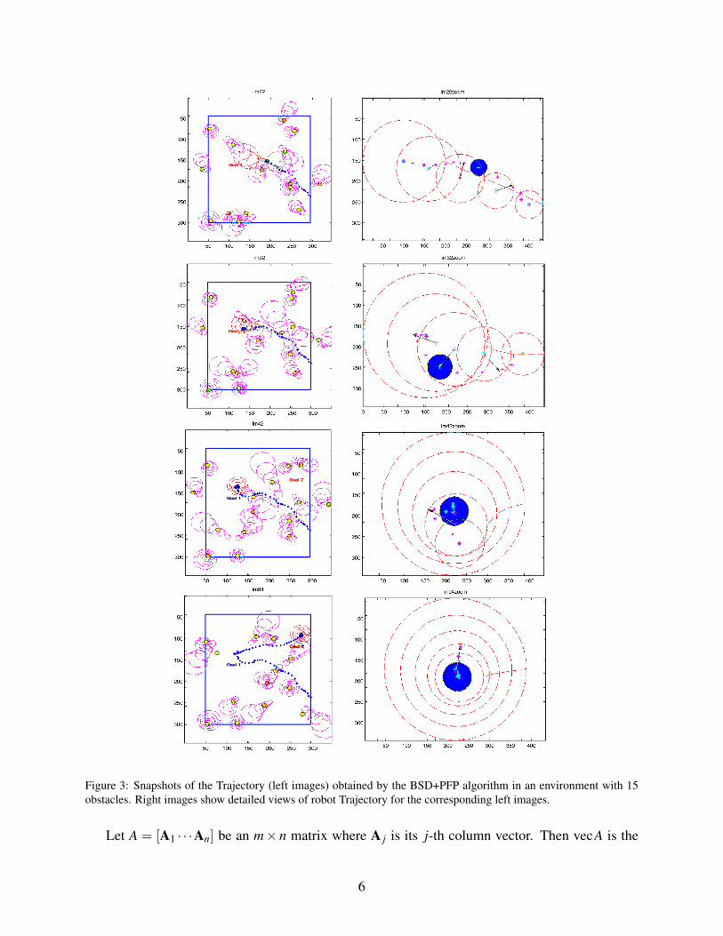
Figure 3: Snapshots of the Trajectory (left images) obtained by the BSD+PFP algorithm in an environment with 15obstacles. Right images show detailed views of robot Trajectory for the corresponding left images.
Let A = [A1 · · ·An] be an m× n matrix where A j is its j-th column vector. Then vecA is the
6

mn×1 vector
vecA =
A1...
An
.Thus the vec operator transforms a matrix into a vector by stacking the columns of the matrix oneunderneath the other. Notice that vecA = vecB does not imply A = B, unless A and B are matricesof the same order. The following properties are useful:
(V1) vecuT = vecu = u, for any column vector u.
(V2) vecuvT = v⊗u, for any two column vectors u and v (not necessarily of the same order).
(V3) Let A, B and C be three matrices such that the matrix product ABC is defined. Then,
vecABC = (CT ⊗A)vecB. (5)
Definition 3. Let F : Rn×q −→ Rm×p be a differentiable function. The Jacobian matrix of F at Xis the mp×nq matrix
DF(X) =∂ vecF(X)
∂ (vecX)T .
Clearly, DF(X) is a straightforward matrix generalization of the traditional definition of theJacobian matrix and all properties of Jacobian matrices are preserved. Thus, the above definitionreduces the study of functions of matrices to the study of vector functions of vectors, since it allowsF(X) and X only in their vectorized forms vecF and vecX . The next properties will be useful (seeChapter 9 in Magnus (2007))
(P1) Assume y = f (X) = X u, such that u is a vector of constants, here f : Rn×m −→ Rn. Thenthe Jacobian matrix is D(Xu) = uT ⊗ I ∈ Rn×nm ∼= R1×m⊗Rn×n.
(P2) Assume y = f (x) = xT x, here f : Rn −→ R. then D(xT x) = 2xT ∈ R1×n.
(P3) Let F : Rn×m −→ Rp×q be defined as F(X) = AXB where A ∈ Rp×n and B ∈ Rm×q arematrices of constants. Then
DF(X) = BT ⊗A. (6)
Theorem 1 (chain rule). Let S be a subset of Rn×q and assume that F : S−→Rm×p is differentiableat an interior point C of S. Let T be a subset of Rm×p such that F(X)∈ T for all X ∈ S, and assumethat G : T −→Rr×s is differentiable at an interior point B=F(C)∈ T. Then the composite functionH : S−→ Rr×s defined by H(X) = G(F(X)) is differentiable at C, and
DH(C) = (DG(B))(DF(C)).
The following theorem will be useful.
7
Theorem 2. Let A be a (p+q)× (p+q)-matrix such that
A =
[A1,1 A1,2−AT
1,2 0
]where A1,1 ∈ Rp×p and A1,2 ∈ Rp×q.
Assume that A1,1 is non-singular, that is, invertible and rankA1,2 = q. Then A is non-singular and
A−1 =
[X1,1 X1,2X2,1 X2,2
],
where X2,2 = (AT1,2A1,1A1,2)
−1,X2,1 = X2,2AT1,2A−1
1,1,X1,1 = A−11,1 − A−1
1,1A1,2X2,1 and X1,2 =
−A−11,1A1,2X2,2.
4. A matrix-based optimization algorithm for shape deformation using a basis of parametriccurves
Now, the aim is the reduction of the cost in computational time of the BSD algorithm becausethis is a critical point in real-time applications and we notice that this computational cost increasedexponentially if the number of the Bezier curves is increased. For that reason, the BSD algorithmis reformulated using tensors.
We will consider for each fixed n ≥ 1 a finite dimensional basis B0,n, . . . ,Bn,n ⊂ L2[0,1] (inparticular, Bi,n are the Bernstein polynomials of degree n when the curve generated is a Beziercurve) and Ω⊂R2 a compact and convex set. Now, assume that for each time t ∈ (0, tend] we havea matrix of Target Points
Tr(t) =[
T1r (t) · · · Tr
r(t)]∈ R2×r
where T jr (t) ∈ Ω,1 ≤ j ≤ r. Our main goal is to construct a map from [0, tend] to C 1([0,1];R2)
given by
t 7→αnt (u) =
n
∑i=0
Pin(t)Bi,n(u); u ∈ [0,1], (7)
where
Pn(t) =[
P0n(t) · · · Pn
n(t)]∈ R2×(n+1),
for each fixed t is a finite set of control points, Pn(0) is previously known and
T1r (t), · · · ,Tr
r(t) ⊂αnt ([0,1]),
for each t ∈ (0, tend]. Observe that we can write (7) in a equivalent matrix form,
αnt (u) = Pn(t)Bn(u);u ∈ [0,1] (8)
whereBn(u) =
[B0,n(u) · · · Bn,n(u)
]T ∈ R(n+1)×1. (9)
Since αnt (u) ∈ R2 we can write its standard euclidean norm as
‖αnt (u)‖2
2 = Bn(u)T Pn(t)T Pn(t)Bn(u), (10)
8
then, for each fixed t, the energy of the u-parametrized curve αnt in C([0,1],R2) can be given by
its L2([0,1],R2)-norm, that is,
‖αnt ‖∆2 =
(∫ 1
0‖αn
t (u)‖22 du)1/2
=
(∫ 1
0Bn(u)T Pn(t)T Pn(t)Bn(u)du
)1/2
. (11)
Assume that for some t ∈ [0, tend) we previously know αnt as αn
t (u) = Pn(t)Bn(u). Then itmoves in a given small interval of time ∆t to a parametric curve αn
t+∆t , by using a set of perturba-tions for each control point, namely
Xn(t +∆t) =[
X0n(t +∆t) · · · Xn
n(t +∆t)]∈ R2×(n+1), (12)
The resultant parametric curve αnt+∆t will be given by,
αnt+∆t(u) = Pn(t +∆t)Bn(u); u ∈ [0,1]. (13)
wherePn(t +∆t) := Pn(t)+Xn(t +∆t). (14)
To compute Xn(t +∆t) we will use the following least action principle: the curve minimize theenergy to move from αn
t to αnt+∆t and it has to pass through the set of Target Points T1
r (t +∆t), . . . ,Tr
r(t +∆t) for a given set of parameter values, namely
0 = ur1 < ur
2 < · · ·< urr−1 < ur
r = 1.
More precisely, we would like to find αnt+∆t such that
min‖αnt+∆t−αn
t ‖2∆2
s. t. αnt+∆t(u
rj) = T j
r(t +∆t) for 1≤ j ≤ r and r ≤ n−1.(15)
In order to write (15) in a equivalent matrix form we introduce the following notation. Let
Brn =
[Bn(ur
1) · · · Bn(urr)]∈ R(n+1)×r,
where we assume that
rankBrn = r = minn+1,r, (16)
holds for the set of parameter values ur1,u
r2, . . . ,u
rr−1,u
rr. Finally, we consider the matrix function
Φn : R2×(n+1)→ R, defined by
Φn(Xn(t +∆t)) =∫ 1
0Bn(u)T Xn(t +∆t)T Xn(t +∆t)Bn(u)du. (17)
Then the miminization problem (15) can be written in a matrix form as:
minXn(t+∆t)∈R2×(n+1)
Φn(Xn(t +∆t)) (18)
s. t. (Pn(t)+Xn(t +∆t))Brn = Tr(t +∆t). (19)
9
By using the vec operator in (19) and the property V3 defined in the equation (5), we obtain auseful equivalent formulation written as
((Brn)
T ⊗ I2)vecXn(t +∆t) = vecTr(t +∆t)−vec(Pn(t)Brn). (20)
Note that the set of constrains of this problem 19 is linear where (Brn)
T ⊗ I2 ∈ R2r×2(n+1). Inconsequence, the map Φn is defined over a convex set. Thus, by proving the convexity of Φn, eachstationary point of Φn over the constrained set will give us an absolute minimum. In particular, thefollowing proposition give us the first and the second derivative of Φn.
Proposition 1. The following statements hold:
(a) DΦn(Xn(t +∆t)) = 2∫ 1
0(Xn(t +∆t)Bn(u))T (Bn(u)T ⊗ I2)du,∈ R1×2(n+1).
(b) (DΦn(Xn(t +∆t)))T = 2(∫ 1
0(Bn(u)T ⊗Bn(u)⊗ I2)du
)vecXn(t +∆t).
(c) D2Φn(Xn(t +∆t)) = 2∫ 1
0(Bn(u)Bn(u)T ⊗ I2)du = 2
(∫ 1
0Bn(u)Bn(u)T du
)⊗ I2. Moreover,
D2Φn(Xn(t +∆t)) ∈ R2(n+1)×2(n+1) is a definite positive symmetric matrix and hence Φn isa convex function over each convex set Ω.
Proof. First, we observe that
DΦn(Xn(t +∆t)) =∫ 1
0D(Bn(u)T Xn(t +∆t)T Xn(t +∆t)Bn(u)
)du. (21)
Let us consider yn = F(Xn(t+∆t)) = Xn(t+∆t)Bn(u) and G(yn) = yTn yn. Then, DF(Xn(t+∆t)) =
Bn(u)T ⊗ I2 and DG(yn) = 2yTn . Thus, by using Theorem 1 we obtain that
D(Bn(u)T Xn(t +∆t)T Xn(t +∆t)Bn(u)
)= 2yT
n(Bn(u)T ⊗ I2
)= 2(Xn(t +∆t)Bn(u))
T (Bn(u)T ⊗ I2),
and this follows statement (a). By using the fact that,
(DΦn(Xn(t +∆t)))T = 2∫ 1
0
((Xn(t +∆t)Bn(u))
T (Bn(u)T ⊗ I2))T
=
= 2∫ 1
0
(Bn(u)T ⊗ I2
)T(Xn(t +∆t)Bn(u)) = 2
∫ 1
0(Bn(u)⊗ I2)(Xn(t +∆t)Bn(u))du ∈ R2(n+1)×1
(22)and taking the vec operator we obtain that,
(DΦn(Xn(t +∆t)))T = 2(∫ 1
0(Bn(u)T ⊗Bn(u)⊗ I2)du
)vecXn(t +∆t), (23)
an it follows (b). To prove (c) note that
D2 (Bn(u)T Xn(t +∆t)T Xn(t +∆t)Bn(u))= 2
(Bn(u)T ⊗ I2
)T (Bn(u)T ⊗ I2). (24)
Since (Bn(u)Bn(u)T ⊗ I2) is definite positive, we obtain that D2Φn(Xn(t + ∆t)) is also definitepositive for all Xn(t +∆t) ∈ R2×(n+1).
10
Moreover, we have the following lemma.
Lemma 1. The matrix∫ 1
0(Bn(u)T ⊗Bn(u)⊗ I2)du is invertible.
Proof. Observe that∫ 1
0(Bn(u)T ⊗Bn(u)⊗ I2)du =
=
∫ 1
0 B0,n(u)B0,n(u)du · · ·∫ 1
0 Bn,n(u)B0,n(u)du∫ 10 B0,n(u)B1,n(u)du · · ·
∫ 10 Bn,n(u)B1,n(u)du
... . . . ...∫ 10 B0,n(u)Bn,n(u)du · · ·
∫ 10 Bn,n(u)Bn,n(u)du
⊗ I2.
Since∫ 1
0Bi,n(u)B j,n(u)du = 〈Bi,n,B j,n〉L2([0,1];R) we have that
G(B0,n, . . . ,Bn,n) =
∫ 1
0 B0,n(u)B0,n(u)du · · ·∫ 1
0 Bn,n(u)B0,n(u)du∫ 10 B0,n(u)B1,n(u)du · · ·
∫ 10 Bn,n(u)B1,n(u)du
... . . . ...∫ 10 B0,n(u)Bn,n(u)du · · ·
∫ 10 Bn,n(u)Bn,n(u)du
is the Gramian matrix of the basis B0,n, . . . ,Bn,n. From Lemma 7.5 of Deusch (2001) we havethat G(B0,n, . . . ,Bn,n) is a non-singular matrix and hence∫ 1
0(Bn(u)T ⊗Bn(u)⊗ I2)du = G(B0,n, . . . ,Bn,n)⊗ I2
in invertible.
In order to characterize the minimum of (18) and (20) we construct the associate Lagrangian
L (Xn(t +∆t),µ) =Φn(Xn(t +∆t))−µT [(Brn)
T ⊗ I2)vecXn(t +∆t)−−vecTr(t +∆t)+vec(Pn(t)Br
n)],
where µ= [µ1 · · ·µ2r]T ∈ R2r. The first order optimality conditions are (20) and
DΦn(Xn(t +∆t))−µT ((Brn)
T ⊗ I2) = 0, (25)
which is obtained by using Proposition 1 (a) and the property (P3) defined by the equation 6. Theequation (25) is equivalent to
(DΦn(Xn(t +∆t)))T − (I2⊗Brn)µ= 0. (26)
Proposition 1 (b) allows us to write the first order optimality conditions as:
2(∫ 1
0(Bn(u)T ⊗Bn(u)⊗ I2)du
)vecXn(t +∆t)− (I2⊗Br
n)µ= 0
((Brn)
T ⊗ I2)vecXn(t +∆t) = vecTr(t +∆t)−vec(Pn(t)Brn),
(27)
11
that we can write in matrix form as
Az(t +∆t) = f(t), (28)
where
A =
2(∫ 1
0(Bn(u)T ⊗Bn(u)⊗ I2)du
)−(I2⊗Br
n)
((Brn)
T ⊗ I2) 0
∈ R(2(n+1)+2r)×(2(n+1)+2r),
z(t +∆t) =[
vecXn(t +∆t)µ
]and f(t) =
[0
vecTr(t +∆t)−vec(Pn(t)Brn)
],
which are in R(2(n+1)+2r).
Proposition 2. Assume that rankBrn = r. Then the matrix A is invertible.
Proof. First at all we remark that
A =
[A1,1 A1,2−AT
1,2 0
]∈ R2(n+1)+2r×2(n+1)+2r,
where
A11 = 2(∫ 1
0(Bn(u)T ⊗Bn(u)⊗ I2)du
)∈ R2(n+1)×2(n+1),
and
A1,2 =−(I2⊗Brn) =
[−Br
n 00 −Br
n
]∈ R2(n+1)×2r.
From Lemma 1 we known that A1,1 is a non-singular matrix. Since rankA1,2 = 2r becauserankBr
n = r, from Theorem 2 the proposition follows.
Now, the algorithm is the following.
1. Construct the matrix A.
2. Consider ∆t =tend
N−1for a fixed N ≥ 2, and write t j = ( j−1)∆t for 1≤ j ≤ N.
3. Obtain the initial control points Pn(t1) and a sample of Target Points Tr(t1), . . . ,Tr(tN) ⊂Ω⊂ R2×r.
4. For j = 1 to N
(a) Compute z(t j+1) as the solution of the linear system Az(t j+1) = f(t j);
(b) Obtain Xn(t j+1) from z(t j+1);
(c) Compute the new control points Pn(t j+1) = Pn(t j)+Xn(t j+1);
12
5. A matrix-based optimization algorithm for Bezier Shape Deformation
Now, we consider that the curve αt ∈ C ([0,1];Ω) is now described by a finite set of con-catenated parametrized Bezier curves αn1
t , . . . ,αnkt constructed with basis functions of dimensions
n1, . . . ,nk, respectively. By using Section 4, each of these curves can be written as
αnit (u) = Pni(t)Bni(u); u ∈ [0,1]; 1≤ i≤ k (29)
where the matrix of the controls points is,
Pni(t) =[
P0ni(t) · · · Pni
ni(t)]∈ R2×(ni+1). (30)
and the matrix of the Bernstein Basis is,
Bni(u) =[
B0,ni(u) · · · Bni,ni(u)]T ∈ R(ni+1)×1. (31)
We assume that
Bi,n j(u) =(
n j
i
)ui(1−u)n j−i, i = 0, . . .n j
are the Bernstein basis polynomials of degree n j for 1≤ j ≤ k. Let us consider for t ∈ (0, tend] andeach 1≤ i≤ k a set of ri-Target Points
Tri(t) =[
T1ri(t) · · · Tri
ri(t)]∈ R2×ri, (32)
where T jri(t) ∈Ω for 1≤ j ≤ ri, and
T1ri(t), . . . ,Tri
ri(t) ⊂αni
t ([0,1]) (33)
for all t ∈ (0, tend]. Moreover, Pni(0) is previously known.In a similar way as in Section 4, we assume that αt , described by αni
t ki=1, is given. Then we
would like to construct αt+∆t from αnit+∆t
ki=1, as follows. Consider
αnit+∆t(u) = Pni(t +∆t)Bni(u); u ∈ [0,1] (34)
where,
Pni(t +∆t) := Pni(t)+Xni(t +∆t) (35)
andXni(t +∆t) =
[X0
ni(t +∆t) · · · Xni
ni(t +∆t)]∈ R2×(ni+1), (36)
for each 1≤ i≤ k−1.Since (33) holds, for each 1≤ i≤ k we will consider
0 = uri1 < uri
2 · · ·< uriri−1 < uri
ri= 1
and the matrixBri
ni=[
Bni(uri1 ) · · · Bni(u
riri)]∈ R(ni+1)×ri. (37)
13
Since αnit+∆t(u
rij ) = T j
ri(t +∆t), for 1≤ j ≤ ri and 1≤ i≤ k, we have
(Pni(t)+Xni(t +∆t))Brini= Tri(t +∆t) for 1≤ i≤ k. (38)
The continuity of αt given by αnit (1−) =α
ni+1t (0+) for 1≤ i≤ k−1, implies that
Pnini(t) = P0
ni+1(t) (39)
holds for 1≤ i≤ k−1. Since αt+∆t ∈ C ([0,1];Ω), from αnit+∆t(1
−) =αni+1t+∆t(0
+) we have
Xnini(t +∆t) = X0
ni+1(t +∆t), (40)
for 1 ≤ i ≤ k− 1. Assume that αn1t (0),αnk
t (1) belong to the boundary of Ω, denoted by ∂Ω, andthat
ddu
αn1t (u)
∣∣u=0+ = V1(t),
ddu
αnkt (u)
∣∣u=1− = Vk(t),
are given data for all t. This equality and the fact that Bi,n j , for 0 ≤ i ≤ n j and 1 ≤ j ≤ k, areBernstein polynomials, implies
n1(P1n1(t)−P0
n1(t)) = V1(t), nk(Pnk
nk(t)−Pnk−1
nk (t)) = Vk(t). (41)
In a similar way, since
ddu
αn1t+∆t(u)
∣∣u=0+ = V1(t +∆t),
ddu
αnkt+∆t(u)
∣∣u=1− = Vk(t +∆t),
and (41) hold we obtain
n1(X1n1(t +∆t)−X0
n1(t +∆t)) = V1(t +∆t)−V1(t), (42)
nk(Xnknk(t +∆t)−Xnk−1
nk (t +∆t)) = Vk(t +∆t)−Vk(t). (43)
To obtain a differentiability condition, that is αt ∈ C 1([0,1];Ω), we assume
ddu
αnit (u)|u=1− =
ddu
αni+1t (u)
∣∣u=0+ . (44)
and thenni(Pni
ni(t)−Pni−1
ni(t)) = ni+1(P1
ni+1(t)−P0
ni+1(t)) (45)
holds for 1≤ i≤ k−1. In a similar way, if we assume that αt+∆t ∈ C 1([0,1];Ω) then,
ni(Xnini(t +∆t)−Xni−1
ni(t +∆t)) = ni+1(X1
ni+1(t +∆t)−X0
ni+1(t +∆t)) (46)
holds for 1≤ i≤ k−1.To conclude, we would like to compute Xni(t +∆t) ∈ R2×(ni+1) for 1≤ i≤ k satisfying
min(Xn1(t+∆t),...,Xnk (t+∆t)) ∑ki=1 Φni(Xni(t +∆t))
s. t. (Pni(t)+Xni(t +∆t))Brini = Tri(t +∆t), 1≤ i≤ k,
Xnini(t +∆t) = X0
ni+1(t +∆t), 1≤ i≤ k−1,
n1(X1n1(t +∆t)−X0
n1(t +∆t)) = V1(t +∆t)−V1(t),
nk(Xnknk(t +∆t)−Xnk−1
nk (t +∆t)) = Vk(t +∆t)−Vk(t),ni(Xni
ni(t +∆t)−Xni−1ni (t +∆t)) = ni+1(X1
ni+1(t +∆t)−X0
ni+1(t +∆t)), 1≤ i≤ k−1,
(47)
14
Introduce the matrix function
Φ(Xn1(t +∆t), . . . ,Xnk(t +∆t)) :=k
∑i=1
Φni(Xni(t +∆t)),
which is a linear combination with positive coefficients of convex functions. In consequence it isalso a convex function over each convex set Ω⊂ (R2×(n1+1)×·· ·×R2×(nk+1)). Moreover,
DΦ(Xn1(t +∆t), . . . ,Xnk(t +∆t)) =[
DΦn1(Xn1(t +∆t)) · · · DΦnk(Xnk(t +∆t))],
where DΦ(Xn1(t +∆t), . . . ,Xnk(t +∆t)) ∈ R1×2∑ki=1(ni+1) and
D2Φ(Xn1(t +∆t), . . . ,Xnk(t +∆t)) = diag
(D2
Φn1(Xn1(t +∆t)), . . . ,D2Φnk(Xnk(t +∆t))
).
By using Proposition 1, we see that D2Φ(Xn1(t +∆t), . . . ,Xnk(t +∆t)) is a definite positive matrix.Now, we would like to write (47) in a more compact notation. To this end we use the followingfour block matrices. For 1≤ i≤ k we define
Rni =[
0 · · · 0 0 I2]∈ R2×2(ni+1),
R∗ni=[
0 · · · 0 −I2 I2]∈ R2×2(ni+1),
Lni =[
I2 0 0 · · · 0]∈ R2×2(ni+1)
and
L∗ni=[−I2 I2 0 · · · 0
]∈ R2×2(ni+1).
Finally, we denote by
0ni =[
0 0 0 · · · 0]∈ R2×2(ni+1),
here and for all the above matrices 0 denotes the square matrix[0 00 0
].
Then by using the above matrices and the vec operator we can write the set of constrains in (47) as
((Brini)
T ⊗ I2)vecXni(t +∆t) = vecTri(t)−vec(Pni(t)Brini), 1≤ i≤ k,
RnivecXni(t +∆t) = Lni+1vecXni+1(t +∆t), 1≤ i≤ k−1,n1L∗n1
vecXn1(t +∆t) = V1(t +∆t)−V1(t),nkR∗nk
vecXnk(t +∆t) = Vk(t +∆t)−Vk(t),niR∗ni
vecXni(t +∆t) = ni+1L∗ni+1vecXni+1(t +∆t), 1≤ i≤ k−1.
(48)
15

Now, the Lagrangian function associated to (47) is
L (Xn1(t +∆t), . . . ,Xnk(t +∆t),λr11 , . . . ,λ
rkk ,µ1, . . . ,µ2k)
= ∑ki=1 Φni(Xni(t +∆t))
−∑ki=1(λ
rii )
T [((Brini)
T ⊗ I2)vecXni(t +∆t)−vecTri(t)+vec(Pni(t)Brini)]
−∑k−1i=1 µ
Ti[RnivecXni(t +∆t)−Lni+1vecXni+1(t +∆t)
]−µT
k
[n1L∗n1
vecXn1(t +∆t)−V1(t +∆t)+V1(t)]
−µTk+1[nkR∗nk
vecXnk−Vk(t +∆t)+Vk(t)]
−∑k−1i=1 µ
Ti+1+k
[niR∗ni
vecXni(t +∆t)−ni+1L∗ni+1vecXni+1(t +∆t)
],
(49)
where,
λrii =
λ 1i...
λ2rii
∈ R2ri, (50)
for 1≤ i≤ k, and
µ j =
[µ1
jµ2
j
]∈ R2, (51)
for 1≤ j ≤ 2k. The first order optimality conditions are given by (48),
DΦn1(Xn1(t +∆t))− (λr11 )
T ((Br1n1)
T ⊗ I2)−µT1 Rn1−µT
k n1L∗n1−µT
k+2n1R∗n1= 0, (52)
DΦni(Xni(t +∆t))− (λrii )
T ((Brini)
T ⊗ I2)−µTi Rni +µT
i−1Lni−µTk+1+iniR∗ni
+µTk+iniL∗ni
= 0,(53)
for 2≤ i≤ k−1, and
DΦnk(Xnk(t +∆t))− (λrkk )
T ((Brknk)
T ⊗ I2)+µTk−1Lnk−µT
k+1nkR∗nk+µT
2knkL∗nk= 0. (54)
Thus, the first order optimality conditions with respect to the vecXni(t +∆t)-variables (52)–(54)can be written respectively as,
0 = 2(∫ 1
0(Bn1(u)
T ⊗Bn1(u)⊗ I2)du)
vecXn1(t +∆t)− (I2⊗Br1n1)λ
r11
−RTn1µ1−n1(L∗n1
)Tµk−n1(R∗n1)Tµk+2,
(55)
0 = 2(∫ 1
0(Bni(u)
T ⊗Bni(u)⊗ I2)du)
vecXni(t +∆t)− (I2⊗Brini)λ
rii
+LTniµi−1−RT
niµi +ni(L∗ni
)Tµk+i−ni(R∗ni)Tµk+i+1,
(56)
16

for 2≤ i≤ k−1.
0 = 2(∫ 1
0(Bnk(u)
T ⊗Bnk(u)⊗ I2)du)
vecXnk(t +∆t)− (I2⊗Brknk)λ
rkk
+LTnkµk−1−nk(R∗nk
)Tµk+1 +nk(L∗nk)Tµ2k.
(57)
Finally, we conclude that the solution of the minimization program (47) can be computed by meansthe following linear system,
Az(t +∆t) = f(t) (58)
where A is a block matrix given by
A =
[A1,1 A1,2A2,1 0
].
The block matrices are
A1,1 = diag(Zn1, . . . ,Znk)
where,
Zni = 2∫ 1
0(Bni(u)
T ⊗Bni(u)⊗ I2)du ∈ R2(ni+1)×2(ni+1)
for i = 1,2, . . . ,k,
A1,2 = [B1 B2 B3 B4] and A2,1 =
C1C2C3C4
.where
B1 = diag(−(I2⊗Br1n1), . . . ,−(I2⊗Brk
nk)),
C1 = diag((Br1n1)T ⊗ I2, . . . ,(Brk
nk)T ⊗ I2),
B2 =
−RTn1
0Tn1
0Tn1
0Tn1· · · 0T
n10T
n1LT
n2−RT
n20T
n20T
n2· · · 0T
n20T
n20T
n3LT
n3−RT
n30T
n3· · · 0T
n30T
n3...
......
... . . . ......
0Tnk−1
0Tnk−1
0Tnk−1
0Tnk−1
· · · LTnk−1
−RTnk−1
0Tnk
0Tnk
0Tnk
0Tnk· · · 0T
nkLT
nk
,
C2 =
Rn1 −Ln2 0n3 · · · 0nk−2 0nk−1 0nk
0n1 Rn2 −Ln3 · · · 0nk−2 0nk−1 0nk...
...... . . . ...
......
0n1 0n2 0n3 · · · Rnk−2 −Lnk−1 0nk
0n1 0n2 0n3 · · · 0nk−2 Rnk−1 −Lnk
,
17
B3 =
−n1(L∗n1
)T 0Tn1
0Tn2
0Tn2......
0Tnk−1
0Tnk−1
0Tnk
−nk(R∗nk)T
,
C3 =
[n1L∗n1
0n2 0n3 · · · 0nk−1 0nk
0n1 0n2 0n3 · · · 0nk−1 nkR∗nk
]
B4 =
−n1(R∗n1)T 0T
n10T
n1· · · 0T
n10T
n10T
n1n2(L∗n2
)T −n2(R∗n2)T 0T
n2· · · 0T
n20T
n20T
n20T
n3n3(L∗n3
)T −n3(R∗n3)T · · · 0T
n30T
n30T
n3...
...... . . . ...
......
0Tnk−1
0Tnk−1
0Tnk−1
· · · 0Tnk−1
nk−1(L∗nk−1)T −nk−1(R∗nk−1
)T
0Tnk
0Tnk
0Tnk
· · · 0Tnk
0Tnk
nk(L∗nk)T
,
and
C4 =
n1R∗n1
−n2L∗n20n3 · · · 0nk−2 0nk−1 0nk
0n1 n2R∗n2−n3L∗n3
· · · 0nk−2 0nk−1 0nk...
...... . . . ...
......
0n1 0n2 0n3 · · · nk−2R∗nk−2−nk−1L∗nk−1
0nk
0n1 0n2 0n3 · · · 0nk−2 nk−1R∗nk−1−nkL∗nk
.
We point out the dimension of the block matrices:
A1,1 ∈ R2∑ki=1(ni+1)×2∑
ki=1(ni+1), B1 ∈ R2∑
ki=1(ni+1)×2∑
ki=1 ri, B2 ∈ R2∑
ki=1(ni+1)×2(k−1),
B3 ∈ R2∑ki=1(ni+1)×4, B4 ∈ R2∑
ki=1(ni+1)×2(k−1),C1 ∈ R2∑
ki=1 ri×2∑
ki=1(ni+1),
C2 ∈ R2(k−1)×2∑ki=1(ni+1),C3 ∈ R4×2∑
ki=1(ni+1) and C4 ∈ R2(k−1)×2∑
ki=1(ni+1),
and hence A ∈ Rp×p for
p = 2k
∑i=1
(ni +1)+2k
∑i=1
ri +2(k−1)+4+2(k−1) = 2k
∑i=1
(ni + ri)+6k. (59)
Since,
C j =−BTj for j = 1,2,3,4, (60)
we can write
A =
[A1,1 A1,2−AT
1,2 0
].
18
Finally, we have
z(t +∆t) =
vecXn1(t +∆t)...
vecXnk(t +∆t)λr1
1...
λrkk
µ1...
µ2k
∈ Rp×1 and f(t) =
V1(t +∆t)−V1(t)0...0
Vk(t +∆t)−Vk(t)vecTr1(t)−vecPn1(t)B
r1n1
...vecTrk(t)−vecPnk(t)B
rknk
0...0
∈ Rp×1.
Next, we will show that A is a non-singular matrix and hence there exists a unique minimumfor our problem.
Proposition 3. Assume that rankBr jn j = r j for 1≤ j ≤ k. Then the matrix A is invertible.
Proof. First, observe thatA1,1 = diag(Zn1, . . . ,Znk).
By Proposition 1 the matrix Zn j is invertible for 1 ≤ j ≤ k and, in consequence, rankA1,1 =
∑kj=1 2(n j +1). Thanks to Theorem 2 the proposition follows if
rankA1,2 = rank(−AT1,2) =
k
∑j=1
2r j +2k,
holds. Observe that k < ∑kj=1 r j < ∑
kj=1(n j + 1). Let us denote by e(i)1 , . . . ,e(i)ni+1 the canonical
basis of Rni+1 for 1≤ i≤ k, and observe that
Rni =[
0 · · · 0 0 I2]= (I2⊗ e(i)ni+1)
T ,
R∗ni=[
0 · · · 0 −I2 I2]= (I2⊗ (e(i)ni+1− e(i)ni ))
T ,
Lni =[
I2 0 0 · · · 0]= (I2⊗ e(i)1 )T
and
L∗ni=[−I2 I2 0 · · · 0
]= (I2⊗ (e(i)2 − e(i)1 ))T ,
19
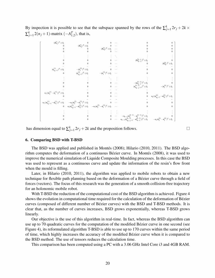
By inspection it is possible to see that the subspace spanned by the rows of the ∑kj=1 2r j + 2k×
∑kj=1 2(n j +1)-matrix (−AT
1,2), that is,
(Br1n1 )
T ⊗ I2 0 0 · · · 0 00 (B
r1n2 )
T ⊗ I2 0 · · · 0 00 0 (B
r2n3 )
T ⊗ I2 · · · 0 00 0 0 · · · 0 0...
.
.
....
. . ....
.
.
.0 0 0 · · · (B
rk−1nk−1 )
T ⊗ I2 0
0 0 0 · · · 0 (Brknk )
T ⊗ I2− − − − − −
(e(1)n1+1)T ⊗ I2 −(e(2)1 )T ⊗ I2 0 · · · 0 0
0 (e(2)n2+1)T ⊗ I2 −(e(3)1 )T ⊗ I2 · · · 0 0
.
.
....
. . ....
.
.
....
0 0 0 · · · −(e(k−1)nk−1 )T ⊗ I2 0
0 0 0 · · · (e(k−1)nk−1+1)
T ⊗ I2 −(e(k)1 )T ⊗ I2− − − − − −
n1((e(1)2 − e(1)1 ))T ⊗ I2 0 0 · · · 0
0 0 0 · · · 0 nk((e(k)nk+1− e(k)nk ))T ⊗ I2
− − − − − −n1((e
(1)n1+1− e(1)n1 ))T ⊗ I2 −n2(e
(2)2 − e(2)1 )T ⊗ I2 0 · · · 0 0
0 n2(e(2)n2+1− e(2)n2 ))T ⊗ I2 −n3(e
(3)2 − e(3)1 )T ⊗ I2 · · · 0 0
.
.
....
.
.
....
.
.
....
0 0 0 · · · −nk−1(e(k−1)2 − e(k−1)
1 )T ⊗ I2 0
0 0 0 · · · nk−1(e(k−1)nk−1+1− e(k−1)
nk−1 ))T ⊗ I2 −nk(e(k)2 − e(k)1 )T ⊗ I2
has dimension equal to ∑kj=1 2r j +2k and the proposition follows.
6. Comparing BSD with T-BSD
The BSD was applied and published in Montes (2008); Hilario (2010, 2011). The BSD algo-rithm computes the deformation of a continuous Bezier curve. In Montes (2008), it was used toimprove the numerical simulation of Liquide Composite Moulding processes. In this case the BSDwas used to represent as a continuous curve and update the information of the resin’s flow frontwhen the mould is filling.
Later, in Hilario (2010, 2011), the algorithm was applied to mobile robots to obtain a newtechnique for flexible path planning based on the deformation of a Bezier curve through a field offorces (vectors). The focus of this research was the generation of a smooth collision-free trajectoryfor an holonomic mobile robot.
With T-BSD the reduction of the computational cost of the BSD algorithm is achieved. Figure 4shows the evolution in computational time required for the calculation of the deformation of Beziercurves (composed of different number of Bezier curves) with the BSD and T-BSD methods. It isclear that, as the number of curves increases, BSD grows exponentially, whereas T-BSD growslinearly.
Our objective is the use of this algorithm in real-time. In fact, whereas the BSD algorithm canuse up to 70 quadratic curves for the computation of the modified Bezier curve in one second (seeFigure 4), its reformulated algorithm T-BSD is able to use up to 170 curves within the same periodof time, which highly increases the accuracy of the modified Bezier curve when it is compared tothe BSD method. The use of tensors reduces the calculation time.
This comparison has been computed using a PC with a 3.06 GHz Intel Core i3 and 4GB RAM.
20

Figure 4: The comparison of the computational cost of BSD and T-BSD methods
7. Conclusions
This work presents a use of tensors which reduces the computational time of the BSD (BezierShape Deformation) algorithm, initially developed within the framework of mobile robotics andliquid composite moulding processes. The result is a tensorial method called T-BSD (Tensor BezierShape Deformation) which enjoys the same properties of the former method including a key ad-vantage: its low computational time and real-time performance. This is a critical issue in someengineering applications. For that reason, the reduction of the execution time of the Bezier gener-ation algorithm is such an important goal to achieve.
In this case of the T-BSD algorithm, the calculation costs depend on the number of curvesrequired to compute a new Bezier from a given one. A field of vectors indicate the direction of de-formation at predefined points in the initial Bezier. The algorithm performs then the concatenationof a set of curves to obtain the deformed Bezier. Besides, the number of curves is highly relatedto the accuracy of the modified Bezier. In fact, the more curves are used the better the accuracy ofthe new Bezier.
As a consequence, the T-BSD algorithm is computed with very low computational time andexcellent accuracy. This is a great outcome in a lot of engineering fields.
A. Ammar, B. Mokdad, F. Chinesta, and R. Keunings: A new family of solvers for some classesof multidimensional partial differential equations encountered in kinetic theory modelling ofcomplex fluids. Journal of Non-Newtonian Fluid Mechanics, 139 3 (2006) 153–176.
C.J. Appellof and E.R. Davidson: Strategies for analyzing data from video fluorometric monitoringof liquid-chromatographic effluents. Analytical Chemistry, 53 13 (1981) 2053–2056.
21

G. Berkooz, P. Holmes, and J. L. Lumley: The proper orthogonal decomposition in the analysis ofturbulent flows. Annual Review of Fluid Mechanics, 25 (1993) 539–575.
E. Cances, V. Ehrlacher, and T. Lelievre: Convergence of a greedy algorithm for high-dimensionalconvex nonlinear problems. In arXiv arXiv1004.0095v1 [math.FA]), April 2010 (to appear inMath. Models and Methods in Appl. Sciences).
J. D. Carroll and J. J. Chang: Analysis of individual differences in multidimensional scaling via ann-way generalization of Eckart-Young decomposition. Psychometrika, 35 (1970) 283–319.
A. Doostan and G. Iaccarino: A least-squares approximation of partial differential equations withhigh-dimensional random inputs. J. Comput. Phys., 228 (12) (2009) 4332–4345.
A. Falco: Algorithms and numerical methods for high dimensional financial market models. Re-vista de Economia Financiera, 20 (2010) 51-68.
W. Hackbusch: Tensor spaces and numerical tensor calculus. Springer series in computationalmathematics, 42. Springer, Heidelber 2012.
T. G. Kolda and B. W. Bader: Tensor decompositions and applications. SIAM Rev., 51 (2009)455–500.
L. De Lathauwer and J. Vandewalle: Dimensionality reduction in higher-order signal processingand rank−(r1,r2, ...,rn) reduction in multilinear algebra. Linear Algebra Appl., 391 (2004) 31–55.
A. Nouy: A generalized spectral decomposition technique to solve a class of linear stochasticpartial differential equations. Computer Methods in Applied Mechanics and Engineering, 96(45-48) (2007) 4521–4537.
A. Nouy: Proper generalized decompositions and separated representations for the numericalsolution of high dimensional stochastic problems. Archives of Computational Methods in Engi-neering, 2010, In press.
L. R. Tucker: Some mathematical notes on three-mode factor analysis. Psychometrika, 31 (1966)279-311.
M. A. O. Vasilescu and D. Terzopoulos: Multilinear analysis of image ensembles: tensorfaces.ECCV 2002:Proceedings of the 7th European Conference on Computer Vision, Lecture Notesin Comput. Sci. 2350, 447–460. Springer, 2002.
G. Vidal: Efficient classical simulation of slightly entangled quantum computations. Phys. Rev.Letters 91 (2003), 147902.
H. Wang and N. Ahuja: Compact representation of multidimensional data using tensor rank-one decomposition. ICPR 2004:Proceedings of the 17th International Conference on PatternRecognition, volume 1, (2004) 44–47.
Graham A. Kronecker Products and Matrix Calculus with Applications. John Wiley, 1981.
22
Magnus J. R. and Neudecker H. . Matrix Differential Calculus with Applications in Statistics andEconometrics: Third Edition. John Wiley and Sons, 2007.
Van Loan C.F. The ubiquitous Kronecker product. J. Comput. Appl. Math. 123 (2000), pp.85-100.
Piegl L. Modifying of the shape of rational B-Spline part 1: Curves. Computer Aided Design,1989, 21(8); 509–518.
Opfer, Oberle G.,H.J. The derivation of cubic splines with obstacles by methods of optimizationand optimal control. Numer.Math.,52,1988;17–31.
Qingbiao Wu, Shuyi Tao. Shape modification of B-Splines curves via constrained optimization formultitarget points. World Congress on Computer Science and Information Engineering, 2009.
Fowler B., Bartels R. Constrained-based curve manipulation. IEEE Computer Graphics and Ap-plication, Vol.13(5),1993;43–49.
Piegl L. On NURBS: A Survey. IEEE Computer Graphics and Applications, 11(1), January1991;55–71.
Au C.K., Yuen M.M.F. Unified approach to NURBS curve shape modification. Computer AidedDesign, 1995, Vol.27(2).
Sanchez R.J. A simple technique for NURBS shape modification. IEEE Computer Graphics andApplications, Vol.17(1),1997;52–59.
Hu S.M., Zhou D.W., Sun J.G. Shape modification of NURBS curves via constrained optimization.Proceedings of the CAD/Graphics, 1999;958–962.
Hu S.M., Zhou D.W., Sun J.G. Modifying the shape of NURBS surfaces with geometric constraints.Computer Aided Design, Vol.33(2),2001;903–912.
Meek D.S.,Ong B.H.,Walton D.J. Constrained interpolation with rational cubics. Computer AidedGeometric Design, Vol.20,2003;253–275.
Deusch F., Best Approximation in Inner Product Spaces CMS Books in Mathematics, Springer–Verlag (2001).
Xu L.,Chen Y.J, Hu N. Shape modification of Bezier curves by constrained optimization. Journalof Software(China), Vol.13(6),2002;1069–1074.
Wu O.B.,Xia F.H. Shape modification of Bezier curves by constrained optimization. Journal ofZhejiang University-Science, Springer-Verlag GmbH,2005;124–127.
Montes N., Sanchez F., Hilario L., Falco A. Flow Numerical Computation through BezierShape Deformation for LCM process simulation methods. International Journal of MaterialForming,Vol.1,2008;919–922.Lyon(France).
Sanchez, F. and Gascon, L.I and Garcia, F.A. and Chinesta, F. On the incubation Time Computa-tion in Resin Transfer Molding Process simulation. International Journal of Forming Processes,2005; 51–67.
23

Mora M.C., Piza R., Tornero J. Multirate obstacle tracking and Path Planning for Intelligent Vehi-cles. IEEE Intelligent Vehicles Symposium, 2007;172–177.
Mora M.C., Tornero J. Planificacion de movimientos mediante la propagacion de campos po-tenciales artificiales. Congreso Iberoamericano de Ingenierıa mecanica, Octava Edicion, 2007october.
Mora M.C.,Tornero J. Path planning and trajectory generation using multi-rate predictive artifi-cial potential-fields. IEEE/RSJ International Conference on Intelligent Robots and Systems, pp.2990-2995, 2008.
Khatib O. Real-time obstacle avoidance for manipulators and mobile robots. The InternationalJournal of Robotics Research,1986, Vol.5 Issue 1;90–98.
Tornero J.,Salt J., Albertos P. LQ Optimal Control for Multirate Sampled Data Systems. IFACWorld Congress, 1999. 14th Edition; 211–216.
Piza R. Modelado del entorno y localizacion de robots moviles autonomos mediante tecnicas demuestreo no convencional. PhD Thesis, Polytechnic University of Valencia, 2003.
Hilario L., Montes N., Falco A., Mora M.C. Real-Time Trajectory Modification Based on BezierShape Deformation. International Conference on Evolutionary Computation, October 2010. Va-lencia (Spain).
Hilario L., Montes N., Mora M.C., Falco A. Real-Time Trajectory Deformation for Poten-tial Fields Planning Methods. IEEE/RSJ International Conference on Intelligent Robots andSystems;1567–1572, September 2011. San Francisco, CA, USA.
24