A Test of the Martingale Hypothesis 1

Joon Y. ParkDepartment of Economics

Rice University and Sungkyunkwan University

and

Yoon-Jae WhangDepartment of Economics

Korea University

Abstract

This paper proposes a statistical test of the martingale hypothesis. It can be used to testwhether a given time series is a martingale process against certain non-martingale alterna-tives. The class of alternative processes against which our test has power is very general andit encompasses many nonlinear non-martingale processes which may not be detected usingtraditional spectrum-based or variance-ratio tests. We look at the hypothesis of martingale,in contrast with other existing methods which test for the hypothesis of martingale differ-ence. Two different types of test are considered: one is a generalized Kolmogorov-Smirnovtest and the other is a Cramer-von Mises type test. For the processes that are first orderMarkovian in mean, in particular, our approach yields the test statistics that neither de-pend upon any smoothing parameter nor require any resampling procedure to simulate thenull distributions. Their null limiting distributions are nicely characterized as functionalsof a continuous stochastic process so that the critical values are easily tabulated. We proveconsistency of our tests and further investigate their finite sample properties via simulation.Our tests are found to be rather powerful in moderate size samples against a wide varietyof non-martingales including exponential autoregressive, threshold autoregressive, markovswitching, chaotic, and some of nonstationary processes.

This version: September 3, 2004

Key words and phrases: Martingale hypothesis, Kolmogorov-Smirnov test, Cramer-vonMises test, Non-linear time series.

1The authors thank for the editor and an anonymous referee for helpful comments. They are alsograteful to Don Andrews, Herman Bierens, Yoosoon Chang, In Choi, Miguel Delgado, Steven Durlauf,Yongmiao Hong, Atsushi Inoue, Peter Phillips, Dongwan Shin and seminar participants at Cowles FoundationEconometrics Conference on New Developments in Time Series Econometrics, October 1999, and at 1999Kamp Econometrics, Pusan, Korea for helpful discussions and comments. The first draft of this paper waswritten while the authors were visiting Cowles Foundation for Research in Economics, whose hospitalityis gratefully acknowledged. Park thanks the Korea Research Foundation for research support, and Whangacknowldeges support provided by the Korea University Research Grant. Address correspondence to: Yoon-Jae Whang, Department of Economics, Korea University, Seoul 136-701, Korea. Phone: +82-2-3290-2224;Fax: +82-2-928-4948; E-mail: whang@korea.ac.kr

1

1. Introduction

In this paper, we introduce a statistical test of the martingale hypothesis. The martingalehypothesis has been considered to be very important in economics and other related fields,since it implies that the best predictor (in the sense of least mean squared errors) of futurevalues of a time series given the current information set is just the current value of thetime series. See, e.g., Hall (1978) for some supportive arguments that consumption isa martingale. The reader is also referred to Durlauf (1991) for more discussions on themartingale hypothesis arising in other contexts of economic theory. Our tests can be usedto test whether a given time series is a martingale process against certain non-martingalealternative processes. The class of alternative processes against which our tests have poweris very general and it encompasses, for example, many interesting nonlinear non-martingaleprocesses including exponential and threshold autoregressive processes, markov switchingand chaotic processes (possibly with stochastic noise), and some of nonstationary processes,see Tong (1990) for more examples of nonlinear time series processes.

We consider two types of tests, which can be regarded as generalizations respectivelyof the Kolmogorov-Smirnov test and the Cramer-von Mises test of goodness of fit to theregression framework. Though they are expected to have discriminatory powers against awide class of non-martingale processes, our tests are very simple to implement in practicalapplications. In particular, if used to test for the martingale hypothesis within the classof first order Markovian processes, the proposed tests become extremely simple to use: thetest statistics are easy to compute and they neither depend upon any smoothing parameternor require any resampling procedure to simulate the null distributions. Their null limitingdistributions are nicely characterized as functionals of a continuous stochastic process. Sincethe distributions are free of any nuisance parameters, we provide a set of critical values whichcan be used readily in practical applications. For the test of the martingale hypothesis in amore general context, they are still free of any nuisance parameters if the test statistics areappropriately formulated, see Section 2 below for a discussion.

Our tests are closely related, among others, to the tests by Durlauf (1991), Hong (1999),Deo (2000), Dominguez and Lobato (2000), and Kuan and Lee (2003). Their tests are, how-ever, not directly comparable to ours, since theirs are the tests of the martingale difference

hypothesis. Durlauf (1991) looks at the spectrum of the first differences and see whether it isconstant. Naturally, his tests are designed to be powerful against all non-martingales gener-ated by serially correlated innovations. For the Gaussian model, the absence of correlation inthe first differences occurs when and only when the underlying process is a martingale. Histest is thus consistent also against all Gaussian non-martingale processes. However, thereare nonlinear non-Gaussian processes which are non-martingales with serially uncorrelatedprocesses [see, e.g., Brockett, Hinich and Patterson (1988, p.658) for an example]. TheDurlauf tests are not expected to have discriminatory powers against such non-martingaleprocesses. Our tests do have powers against such nonlinear non-Gaussian non-martingales,and are more general than his in this respect. On the other hand, Hong (1999) suggestsa test for the martingale hypothesis based on the so-called generalized spectral derivative.His test does have powers against non-linear non-Gaussian non-martingales but it mightbe sensitive to choice of smoothing parameters in practice. Furthermore, the test requires

2

the innovation sequence to be strictly stationary, whereas our tests allow some degree ofheterogeneity of the innovations. See Section 2 for a more discussion on comparison betweenour tests and the existing tests of the martingale difference hypothesis.

We also note that there is a huge literature related to the testing problem consideredhere. One branch of the literature deals with testing for a unit root [see, e.g., Stock (1994) orPhillips (1997) for a survey on the subject]. The unit root hypothesis, however, is obviouslymore general than our martingale hypothesis. Also, the alternatives considered by mostof the existing unit root tests are much more restrictive than ours: Their alternatives areusually stationary linear autoregressive processes, whereas our alternatives allow generalnonlinear processes which might be either stationary or nonstationary. Therefore, we believethat our tests would deliver further insight on the property of a given time series, especiallywhen the underlying data generating mechanism is nonlinear. The other branch of therelated literature consists of the nonlinearity tests for time series. Examples of such testsinclude, among others, An and Bing (1991), Brockett, Hinich, and Patterson (1988), Chanand Tong (1986), Hinich (1982), Hjellvik and Tjøstheim (1995) and Koul and Stute (1999),Luukkonen, Saikkonen, and Terasvirta (1988).2 Some of these tests are also consistentagainst general nonlinear alternatives, but they only look at stationary null and alternativehypotheses. Our tests consider nonstationary processes. To the best of our knowledge, theasymptotic behavior of the nonlinearity tests for nonstationary processes has not yet beeninvestigated. Our tests are also related to the model specification tests by Bierens(1990),Bierens and Ploberger (1997) and de Jong (1996), see the next section for more discussions.

The remainder of this paper is organized as follows. Section 2 introduces the null andalternative hypotheses and defines the test statistics. In Section 3, we derive the asymptoticnull distributions of the test statistics and tabulate their critical values. Section 4 considersthe consistency of our tests. In particular, we establish the consistency of our tests againstgeneral non-martingales that are asymptotically stationary. The test consistency againstsome nonstationary non-martingales is also discussed. Section 5 reports some simulationresults, and Section 6 contains the proofs for the theorems in the main text.

2. The Hypotheses and Test Statistics

Let a time series (yt) be given, and let (Ft) be a filtration to which (yt) is adapted. Thenull hypothesis of interest is that (yt) is a martingale process with respect to the filtration(Ft), i.e.,

H0 : P(E(yt|Ft−1) = yt−1) = 1 (1)

for each t ≥ 1, where E(·|Ft−1) denotes as usual the conditional expectation given Ft−1.The alternative hypothesis is the negation of (1). To test the hypothesis (1), it is of courseessential to further specify the filtration (Ft). For many applications, the most relevantchoice of (Ft) appears to be the natural filtration of (yt), in which case Ft for each t ≥ 1 isdefined to be the σ-field generated by (ys) for all s ≤ t. Different specifications of (Ft), which

2Some of these tests are used to check the departures in each moment, while ours concentrate on testingfor serial dependence in mean.

3

may in particular include other covariates, are also possible and can be more interestingchoices.

In this paper, we mainly consider the simple case in which

E(yt|Ft−1) = E(yt|yt−1) (2)

for all t ≥ 1, see below for a discussion on its multivariate generalization. Clearly, (2) holdsif (yt) is first order Markovian. We call (yt) the first order Markovian-in-mean if it satisfies(2). Note that, as shown in, e.g., Billingsley (1995, Theorem 16.10 (iii), p.213),

E(4yt|yt−1) = 0 a.s. iff E4yt1{yt−1 ≤ x} = 0 for almost all x ∈ R, (3)

where and elsewhere in the paper we denote by 4 the usual difference operator (i.e., 4yt =yt − yt−1) and by 1{·} the indicator function. On the other hand, (3) implies that, whenP(E(4yt|yt−1) = 0) < 1, i.e., when (1) is not true, we have E4yt1{yt−1 ≤ x} 6= 0 for somex ∈ R, see Section 4 below for more details. This motivates us to consider the following asthe basis of our test statistics for the martingale hypothesis (1)3:

Qn(x) =1√n

n∑

t=1

4yt1{yt−1 ≤ x}. (4)

Of course, our assumption (2) can be too restrictive for some applications. To deal withmore general processes, we may wish to look at the case

E(yt|Ft−1) = E(yt|yt−1, . . . , yt−κ) (5)

for all t ≥ 1, with some κ ≥ 2. Similarly as above, we may call (yt) the κ-th order

Markovian-in-mean if it satisfies (5). In this case, we may use the statistics based on

Qn(x1, . . . , xκ) =1√n

n∑

t=1

4yt1{yt−1≤x1} · · · 1{yt−κ≤xκ} (6)

in place of Qn(x) introduced in (4) to more effectively discriminate our martingale nullhypothesis against nonmartingale alternatives. Clearly, Qn(x) in (4) may be regarded asa special case κ = 1 of Qn(x1, . . . , xκ) defined in (6). We may consider even more generalcases where (Ft) includes the information from other covariates in a similar way. Moreover,it is also conceivable to increase κ in (5) and (6) as the sample size grows. All thesegeneralizations and extensions, however, will not be pursued in this paper. They requiresome new development of the functional central limit theory, and will therefore be reportedin our subsequent work.

3In the specification testing literature, Stinchcombe and White (1988, p.299) call the class of indicatorfunctions (1{x ≤ t}, t ∈ R) as the totally revealing set. Examples of specification tests that are based on thisclass of functions include An and Bing (1991), Delgado (1993), Andrews (1997), Stute (1997) and Whang(2000). On the other hand, other choices of function classes are possible (e.g., the exponential functionsused by Bierens (1990), but the indicator function has an advantage that it does not require an arbitrarychoice of a nuisance parameter space.

4

We assume that the time series (4yt) are martingale differences with non-vanishingvariances, as will be more formally introduced in the next section. Roughly, this implies that(yt) becomes a nonstationary integrated process. The formulation in (6) clearly distinguishesthe tests of the martingale hypothesis from those of the martingale difference hypothesis. Wehave to deal with the levels for the former, while we may rely only on the first differences forthe latter.4 There is a large class of models used in economic and financial applications thatspecify the mean changes as functions of the lagged levels rather than the lagged differences,including, for instance, threshold autoregressive models, (both linear and nonlinear) errorcorrection models and various diffusion models. As will be seen clearly in later sections,our tests for the martingale hypothesis yield asymptotics that are very different from thosefor the existing tests of the martingale difference hypothesis. This is mainly due to thepresence of the lagged level in our test statistics.

We may construct two different types of statistics from Qn(x) defined in (4). A Kolmogorov-Smirnov type statistic is given by

Sn = supx∈R

|Qn(x)|. (7)

Moreover, a Cramer-von Mises type statistic is defined as

Tn =

∫

Q2n(x)µn(dx),

where µn denotes some measure. In this paper, we define µn to be the empirical distributionof (yt−1), in which case Tn reduces to

Tn =1

n

n∑

t=1

Q2n(yt−1). (8)

See, e.g., Shorack and Wellner (1986) for other choices of µn.The martingale hypothesis is intimately related to the unit root hypothesis, though

strictly speaking none of them generally implies the other.5 It therefore seems interestingto compare our tests with the unit root test by Dickey and Fuller (1979). Their test is mostcommonly used to test for the unit root. The test relies on the t-statistic on the coefficientβ in the regression

4yt = βyt−1 + εt ,

where (εt) is assumed to be martingale differences. We may thus expect that the testhas some discriminatory powers against our alternatives, which may be reformulated as

4After the first draft of our paper was written, Dominguez and Lobato (2000) proposed a test of thehypothesis E(4yt|4yt−1, . . . ,4yt−p) = 0 a.s. against its negation. The test also uses the indicator functionas the weight function, similary to ours. Their test can indeed be viewed as the test of the martingaledifference hypothesis, corresponding to our tests of the martingale hypothesis.

5Here we use the term ‘unit root’ as defined in Stock (1994) or Phillips (1997). The unit root processwith correlated innovations is in general not a martingale. Conversely, the martingale whose differencesvanishing asymptotically is not a unit root process. We, however, are mostly concerned with the unit rootmartingales in the paper.

5

E(4yt|Ft−1) 6= 0. The test, however, concentrates on one possible violation of the martin-gale hypothesis, i.e., the one into the direction spanned linearly by yt−1, as is the case for thestationary first order autoregression. In contrast, our tests look into many other nonlineardirections as well for the violation of the martingale hypothesis. Our generalization in (5),of course, can be similarly compared with the augmented Dickey-Fuller test.

If the martingale difference hypothesis, not the martingale hypothesis, is what we wantto test, it can also be done using the approaches taken by Bierens (1990) and de Jong (1996)in a broader context of general model specifications. In particular, the test proposed by deJong (1996) can be used to test the martingale difference hypothesis

E(4yt|4yt−1, . . . ,4y1) = 0 a.s.

with the natural filtration, if it is applied to the first differences (4yt). However, de Jong(1996)’s test appears not to be very attractive in our context. His test is a bit too general,and hence has very low power in small samples as is indicated by the author. Furthermore,his test is computationally very demanding since it depends on high dimensional integrationand cumbersome Monte Carlo simulations.

3. The Null Distributions

In this section, we derive the null distributions of the test statistics Sn and Tn introducedin the previous section. We let

ut = 4yt

and define (Ft) to be the filtration introduced earlier. Throughout this section, we supposethat (yt) is first order Markovian-in-mean. The condition in (2) therefore holds. We assume

3.1 Assumption (ut,Ft) is a martingale difference sequence such that

(a)1

n

n∑

t=1

E(

u2t

∣

∣Ft−1

)

→p σ2 > 0, and

(b) supt≥1

E(

u4t

∣

∣Ft−1

)

< K a.s. for some constant K < ∞.

Note that the condition in the part (a) of Assumption 3.1 allows the innovation sequence(ut) to be heteroskedastic, conditionally and/or unconditionally, as long as it is averagedout in the limit. It is satisfied for instance by the martingales driven by ARCH-type in-novations. The part (b) of Assumption 3.1 requires that the fourth conditional moment isuniformly bounded.6 The condition implies in particular the conditional version of Linder-

6Strictly speaking, Assumption 3.1(b) rules out the standard GARCH(1,1) process. However, this as-sumption is standard in the nonstationary time series literature (see, e.g. Stock (1994)) and we believe thatthis assumption is not entirely necessary for our asymptotic results to hold. Furthermore, our simulationexperiments in Section 5 show that our tests have good size and power performance in the presence ofGARCH errors.

6

berg condition, i.e.,

1

n

n∑

t=1

E(

u2t 1{|ut| > ε

√n}∣

∣Ft−1

)

→p 0

as n → ∞ for any ε > 0, which is routinely imposed to obtain the martingale limit theory.Under Assumption 3.1, the usual variance estimator σ2

n = (1/n)∑n

t=1 u2t of (ut) is

consistent for its asymptotic variance σ2, i.e., σ2n →p σ2, which we state formally as a

lemma.

3.2 Lemma Let Assumption 3.1 hold. Then we have σ2n →p σ2 as n → ∞.

In what follows, we assume that σ2 = 1 and (ut) is normalized so that σ2n = 1. Of course,

the normalization can be done by dividing (yt) by σn.7 This is to ease the exposition of ourtheory. Given the consistency of σ2

n in Lemma 3.2, the convention imposes no restrictionon our subsequent theory.

Let

Wn(r) =1√n

[nr]∑

t=1

ut (9)

for 0 ≤ r ≤ 1, where [z] is the largest integer which does not exceed z. Under Assumption3.1, invariance principle holds, as shown by, e.g., Hall and Heyde (1980, Theorem 4.1, p.99). More precisely, we have the weak convergence

Wn →d W (10)

in D[0, 1], the space of cadlag functions on [0, 1], endowed with the Skorohod topology,where W is the standard Brownian motion.

Now we defineMn(x) = Qn(x

√n). (11)

We may write Sn asSn = sup

x∈R

|Mn(x)|. (12)

Moreover, we have

Tn =

∫ 1

0M2

n(Wn(r)) dr, (13)

where Wn is the process introduced in (9).From now on, we regard Mn defined in (11) as a stochastic process with parameter

x ∈ R. It takes values in D(R), i.e., the space of cadlag functions on R. As before, we

7The normalized sequences should be more precisely denoted by (ynt) and (unt), since they depend uponn. We will, however, continue to use (yt) and (ut) to simplify the notation

7

endow D(R) also with the Skorohod topology. We now write the process Mn introduced in(11) as

Mn(x) =1√n

n∑

t=1

ut 1

{

yt−1√n

≤ x

}

=

∫ 1

01{Wn(r) ≤ x} dWn(r)

for x ∈ R. We may extend the definition of Mn to ±∞ by putting

Mn(−∞) = 0 and Mn(∞) =1√n

n∑

t=1

ut = Wn(1).

Then, Mn becomes a process taking values in D[−∞,∞] which, up to a strictly increasingcontinuous transformation, is the same as D[0, 1].

Given the weak convergence (10) of Wn to W in D[0, 1], it is well expected that thestochastic process Mn weakly converges as n → ∞ in D[−∞,∞] to M defined by

M(x) =

∫ 1

01{W (r) ≤ x} dW (r) (14)

for x ∈ R with M(−∞) = 0 and M(∞) = W (1). The weak convergence is presented in thefollowing lemma.

3.3 Lemma Under Assumption 3.1, we have Mn →d M in D[−∞,∞] as n → ∞.

The asymptotic distributions of the statistics Sn and Tn can now be readily derived fromthe result in Lemma 3.3 and the continuous mapping theorem, since they are continuousfunctionals of Mn.

3.4 Theorem Suppose that Assumption 3.1 holds. Then, we have

Sn →d S = supx∈R

|M(x)|

Tn →d T =

∫ 1

0M2(W (r)) dr

as n → ∞.

The proof of the above theorems and some of our subsequent results involves the localtime of the limit Brownian motion W , which we denote by L(t, s) with t and s signifyingrespectively the time and space parameters. It may be defined as

L(t, s) = limε→0

1

2ε

∫ t

01{|W (r) − s| ≤ ε} dr (15)

8

Figure 1: Probability Density of S

and can be interpreted as the time spent by W , up to time t, in the immediate vicinity ofthe level s. The local time L yields the equality

∫ t

0F (W (r)) dr =

∫ ∞

−∞F (s)L(t, s) ds

for any locally integrable function F : R → R, which is known as the occupation timesformula. The reader is referred to Chung and Williams (1990) for an introduction to theBrownian local time and occupation times formula.

We also need to further investigate the properties of the limit process M to fully under-stand the asymptotic properties of the test statistics Sn and Tn.

3.5 Lemma We have for any p ≥ 2 and x, y ∈ R,

E|M(x) − M(y)|p ≤ cp|x − y|p/2,

where cp is a constant depending only upon p.

3.6 Proposition There is a modification of M , whose paths are Holder continuous oforder p ∈ [0, 1/2).

We may therefore assume that M is a continuous stochastic process.Since the process M is continuous and effectively stopped at

smin = infr∈[0,1]

W (r) and smax = supr∈[0,1]

W (r),

i.e., M(x) = M(smin) = 0 for all x ≤ smin and M(x) = M(smax) = W (1) for all x ≥ smax, itis obvious that the limit random variable S introduced in Theorem 3.4 is a.s. well defined.

9

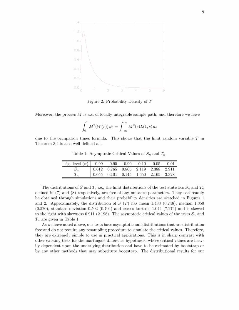
Figure 2: Probability Density of T

Moreover, the process M is a.s. of locally integrable sample path, and therefore we have

∫ 1

0M2(W (r)) dr =

∫ ∞

−∞M2(s)L(1, s) ds

due to the occupation times formula. This shows that the limit random variable T inTheorem 3.4 is also well defined a.s.

Table 1: Asymptotic Critical Values of Sn and Tn

sig. level (α) 0.99 0.95 0.90 0.10 0.05 0.01

Sn 0.612 0.765 0.865 2.119 2.388 2.911Tn 0.055 0.101 0.145 1.650 2.165 3.328

The distributions of S and T , i.e., the limit distributions of the test statistics Sn and Tn

defined in (7) and (8) respectively, are free of any nuisance parameters. They can readilybe obtained through simulations and their probability densities are sketched in Figures 1and 2. Approximately, the distribution of S (T ) has mean 1.433 (0.746), median 1.350(0.520), standard deviation 0.502 (0.704) and excess kurtosis 1.044 (7.274) and is skewedto the right with skewness 0.911 (2.198). The asymptotic critical values of the tests Sn andTn are given in Table 1.

As we have noted above, our tests have asymptotic null distributions that are distribution-free and do not require any resampling procedure to simulate the critical values. Therefore,they are extremely simple to use in practical applications. This is in sharp contrast withother existing tests for the martingale difference hypothesis, whose critical values are heav-ily dependent upon the underlying distribution and have to be estimated by bootstrap orby any other methods that may substitute bootstrap. The distributional results for our

10

tests are, of course, not directly comparable to those for the existing martingale differencetests. The former include the lagged level that is nonstationary, while the latter only con-sider the lagged differences that are assumed to be stationary. The distribution-free natureof our tests is not particularly due to the first order Markovian-in-mean structure of themodel that we consider in the paper. They continue to be independent of the underlyingdistribution if we consider the statistic (6) for the general κ-th order Markovian-in-meanmodel (5). The details will be reported in our subsequent work.

4. Consistency of the Tests

In this section, we establish consistency of our tests based on the statistics Sn and Tn againstcertain non-martingale alternatives.

Suppose, for now, that (yt) is strictly stationary. By definition, (yt) is in the alternativehypothesis if it satisfies

P(E(4yt|yt−1) 6= 0) > 0. (16)

Note that (16) is equivalent to (17):

E4yt1{yt−1 ≤ x} =

∫

E(4yt|yt−1 = z)1{z ≤ x} dP(z) (17)

6= 0 for some x ∈ R,

where P denotes the time invariant stationary distribution of (yt). Therefore, we can seethat the tests based on the sample analogue of (17) might be consistent againt generalalternatives satisfying (16). This is shown in Theorem 4.4 below.

We now relax the assumption of strict stationarity. To allow for some degree of hetero-geneity of alternative processes, we write explicitly the random variables (yt) to be trian-gular arrays, i.e., (ynt) for n ≥ 1 and 1 ≤ t ≤ n. By definition, (ynt) is in the alternativehypothesis if it satisfies:

4.1 Assumption Assume that we have, for all z ∈ R, (1/n)∑n

t=1 E(4ynt|yn,t−1 = z) →H(z) as n → ∞, where H is a measurable function on R, and that we have, for anyBorel set A ⊂ R, (1/n)

∑nt=1 Pnt(A) → P(A) as n → ∞, where P is a probability measure

on R and Pnt are the distributions of (ynt) for 1 ≤ t ≤ n, n ≥ 1. Furthermore, we let∫

1{H(z) 6= 0} dP(z) > 0.

Clearly, Assumption 4.1 includes (16) as a special case and is easy to check in practice. Forexample, suppose (yt) is a stationary AR(1) process, i.e., yt = αyt−1 +εt, where |α| < 1 and(εt) are i.i.d. (0, σ2). Then we have H(z) = E(4yt|yt−1 = z) = (α − 1)z and P becomesthe time invariant stationary distribution of (yt). In this case, Assumption 4.1 holds unlessP is degenerate and puts mass 1 at the origin (in which case we have yt = 0 a.s. for all t).Similarly, suppose (yt) is a deterministically trending process, i.e., yt = α0 + α1(t/n) + εt,where (εt) are i.i.d. U [−1, 1]. Then, H(z) = limn→∞(1/n)

∑nt=1 E(4yt|yt−1 = z) = −z +

α0 +α1/2 and P is given by the uniform distribution U [α0−(1−α1)/2, 1+α0−(1−α1)/2].In this case also, Assumption 4.1 holds with

∫

1{H(z) 6= 0} dP(z) = 1

11

We further assume that the triangular array of random variables (ynt) is weakly depen-dent and satisfies a moment condition.

4.2 Assumption Assume that (ynt) is a strong mixing triangular array that satisfiessupn≥1,1≤t≤n E|4ynt|p < ∞ for some p ∈ [1,∞].

This assumption might be relaxed along the lines discussed below, if needed.For our consistency result, we need the following uniform Weak Law of Large Numbers

(WLLN):

4.3 Lemma Under Assumption 4.2, we have

supx∈R

∣

∣

∣

∣

∣

1

n

n∑

t=1

[4ynt1{yn,t−1 ≤ x} − E4ynt1{yn,t−1 ≤ x}]∣

∣

∣

∣

∣

→p 0 (18)

as n → ∞.

Consistency of our tests is established in the following theorem:

4.4 Theorem Suppose that Assumptions 4.1 and 4.2 hold with p ≥ 2. Then, we have

Sn, Tn →p ∞

as n → ∞.

Theorem 4.4 shows that the tests Sn and Tn are consistent if we reject the null hypothesiswhen they take large values.

4.5 Remarks (a) The strong mixing assumption and Lp-boundedness condition in As-sumption 4.2 were assumed to use the pointwise WLLN result of Andrews (1988, exam-ple 4, p.462), see proof of Theorem 4.4 and Lemma 4.3 below. They can be relaxed ifneeded. For example, to allow for trending random variables, one can use the result ofde Jong (1995, Theorems 1 or 3) to verify the pointwise WLLN which requires the trian-gular array of random variables (4ynt1{yn,t−1 ≤ x}) and (4y2

nt) minus their respectivemeans are Lq-mixingale or Lq-near epoch dependent on some strong mixing sequence with1 ≤ q ≤ 2 and satisfy other additional moment conditions in the Theorems. In this case, thebracketing condition (33) in the proof of Lemma 4.3 can be verified under the assumptionlim supn→∞(1/n)

∑nt=1 E|4ynt|p < ∞ for some p > 1.

(b) Lemma 4.3 gives a uniform WLLN for unbounded and non-differentiable functionsof weakly dependent and non-identically distributed random variables. To the best of ourknowledge, such result is not yet available in the literature and hence would be of separateinterest. This lemma also differs from the uniform WLLN of Koul and Stute (1999, equation(4.1)) who assume stationarity of the random variables whereas we allow for heterogeneousrandom variables.

12

The alternatives we consider in Assumptions 4.1 and 4.2 are processes that are essen-tially stationary. Though we allow for quite flexible forms of nonstationarity there, it isrequired that the nonstationarity be vanished asymptotically. Unfortunately, it does notseem possible to obtain any general theoretical results for the powers of our tests againstthe non-martingale processes with non-vanishing nonstationarity. Our tests may or maynot have powers against such non-martingales that are intrinsically nonstationary. Amongthe processes we consider in our simulations reported in the next section, Sn appears tohave desirable power against the explosive process that is intrinsically nonstationary. Onthe other hand, both Sn and Tn fail to have effective powers against many non-martingaleunit root processes. For the intrinsically nonstationary models, (16) does not warrant theconsistency of our tests, even if it holds for all t ≥ 1. If (yt) is nonstationary even asymp-totically, our tests may become inconsistent against the non-martingale alternatives. Wemay indeed show that the basis of our tests Qn, introduced in (4), does not diverge undermany unit root non-martingale alternatives.8

To see this, we first consider the simple random walk (yt) given by 4yt = ut, where (ut)is an i.i.d. innovation sequence with mean zero and unit variance. As shown in Chang andPark (2004), we have for this process

1√n

n∑

t=1

ut1{yt ≤ 0} →d M(0) + KL(1, 0), (19)

where M is the process defined in (14), K > 0 is some constant and L is the local timegiven in (15). We may compare the result in (19) with Lemma 3.3 to understand the effectsof the presence of dependency in the innovation ut and the argument yt in the indicatorfunction. The dependency does not change the rate of convergence. However, it alters thelimit distribution, and in particular, it shifts the limit distribution to the right by KL(1, 0).Note that L(1, 0) > 0 a.s.

We now look at the non-martingale unit root process (yt) generated by 4yt = ut with(ut) that is serially correlated. The result in (19) for the simple random walk gives us anobvious clue on how our tests would behave for this class of nonmartingales. Note thatut is correlated with yt−1 when (ut) are serially correated, so in this case we may expectthat our tests have the asymptotics similar to (19). Therefore, it is clear that our testsare generally inconsistent for the unit root nonmartingales driven by serially correlatedinnovations. Yet, we may predict that our tests would have some nontrivial powers againstsuch non-martingales, since the presence of serial correlation in (ut) would shift the limitdistributions of our tests. The appearance of the additional term involving L(1, 0) in (19) isdue to the nonzero correlation of ut and yt, and we may see that a similar term will appearin our case here. In fact, this is exactly what we observe in our simulation study.

8For the unit root non-martingales, the conditional expectation E(4yt|Ft−1) is generally given as afunction of the lagged differences 4yt−1,4yt−2, . . ., and in particular, our maintained assumption (2) doesnot hold. Therefore, strictly speaking, they are not allowed in our framework. To test the martingalehypothesis against such alternatives, it seems preferred to use any of the existing martingale difference tests.

13

5. Simulation Results

In this section, we examine the finite sample performance of our tests in a small scalesimulation experiment. We choose ten different models as described in Table 2 to generatesimulated data. Model NULL generates random walk processes possibly with GARCHerrors and is considered to evaluate the size performance of our tests. The other models areconsidered to see the power performance of our tests.

Table 2. Data Generating Processes

Model DGP (εt ∼ i.i.d. N(0, 1))

NULL yt = yt−1 + ut; ut = σtεt, σ2t = 1 + θ1u

2t−1 + θ2σ

2t−1

ARMA yt = θ1yt−1 + θ2εt−1 + εt

EXAR yt = θ1yt−1 + θ2yt−1 exp (−0.1 |yt−1|) + εt

TAR yt = θ1yt−11{|yt−1| < θ2} + 0.9yt−11{|yt−1| ≥ θ2} + εt

BL yt = θ1yt−1 + θ2yt−1εt−1 + εt

NLMA yt = θ1yt−1 + θ2εt−1εt−2 + εt

MARKOV yt − µst= θ1(yt−1 − µst−1

) + εt, st = 0 or 1, µ0 = 0, µ1 = 1.θ2 = P (st = 0|st−1 = 0) = P (st = 1|st−1 = 1)

FM yt = mt + ut; mt = θ1yt−1(1 − yt−1), ut = θ2vtηt,vt = min{mt, 1 − mt}, ηt ∼ i.i.d. Uniform(0, 1)

EXP yt = θ1yt−1 + ut; |θ1| > 1, ut = σtεt, σ2t = 1 + θ2u

2t−1 + θ3σ

2t−1

UNIT yt = yt−1 + ut; ut = θ1ut−1 + εt

TREND yt = θ1 + θ2(t/n) + yt−1 + εt

Model ARMA generates an autoregressive moving average process of order (1,1). ModelEXAR is an exponential autoregressive model. Model TAR is a threshold autoregressivemodel of order 1. This model can capture the possibility of asymmetric movements in a timeseries, see Tong (1990, Section 3.3).9 Model BL is a bilinear model. This model introducescoefficients that are linear function of the error term and is considered to lie somewherebetween the “fixed coefficient” autoregressive models and the “random coefficient” autore-gressive models, see also Tong (1990, p.114). Model NLMA is a nonlinear moving averagemodel. Model MARKOV is a markov switching model, see Hamilton (1989) for motivation.Model FM is a Feigenbaum map with system noise. When θ1 = 4, this map generates achaotic process which is a globally bounded but locally explosive stationary process, see forexample Whang and Linton (1999) and the references therein for discussions about chaoticprocesses. Model EXP is an explosive AR(1) model and Model UNIT is a unit root processwith an AR(1) innovation sequence. Finally, Model TREND is a random walk model witha deterministic trend.

In each of the model, we generate (εt) independently from the standard normal distribu-tion and set the initial values, e.g., y0, ε0, ε−1 to zero. A total of 1,000 replications are usedfor each experiment. We take n = 100, 250, 500, 1000 and report for each n the rejection

9We have also considered momentum threshold autoregressive models (or MTAR models), which areintroduced by Enders and Granger (1998), but the simulation results were similar to those of TAR andhence are not reported here.

14

probabilities of the test with nominal size α = 0.05. The results corresponding to differentnominal sizes were similar and hence are not reported.

Tables 3-13 present the rejection probabilities of our tests based on the statistics Sn andTn. We compare the performance of our tests with the Cramer-von Mises type test of themartingale hypothesis proposed by Durlauf (1991), denoted as CVMn.10

Table 3 shows that our tests, designated as Sn and Tn, have reasonably good size per-formance and the size performance is little affected by the GARCH structure of the errors.On the other hand, the test CVMn tends to over-reject when the errors follow GARCHprocesses.11

Tables 4-13 report the finite sample performances of our tests against a wide variety ofalternative non-martingale processes. The performances of our tests are reasonably good ingeneral, but they are somewhat critically dependent upon the underlying data generatingprocesses.

Table 4 considers the case of the ARMA(1,1) process. The overall performance of ourtests against the stationary ARMA processes appears to be reasonably good. However, theperformances of our tests against the near-unit root process are somewhat unsatisfactoryespecially when the sample size is small. When the autoregressive coefficient is close tounity, i.e., θ1 = .95, our tests indeed do not seem to have any discriminatory power insamples of size less than n = 250. Though it is also far from being satisfactory, the Durlauftest has better powers than our tests in small samples. The comparison, however, is reverseddrastically as the sample size increases. For the samples as large as n = 1, 000, our testsSn and Tn, especially the one based on Tn, have effective discriminating powers againstthe near-unit root alternative. The power of the Durlauf CVMn test, however, improvesonly very slowly as the sample size increases. When there is a moving average component,i.e., θ2 6= 0, the performances of all three tests become slightly worse but, nevertheless, thecomparison between our tests Sn and Tn with the Durlauf CVMn remains to be largely thesame.

Table 5 gives the rejection probabilities when the data are generated from exponentialautoregressive processes. It shows that both Sn and Tn perform well for samples of mod-erately large size. In particular, their performances are substantially better than that ofCVMn in large samples. For samples of small size, however, CVMn performs better than Sn

and Tn in several cases. As for the case of the stationary ARMA alternatives, performancesof our tests Sn and Tn improve rapidly as the sample size increases. This is not so for theDurlauf CVMn test. The power of CVMn increases only very slowly.

Table 6 shows that our tests are consistent against threshold autoregressive models.The rejection probabilities increase as θ1 decreases (i.e., more asymmetry exists) or as θ2

increases (i.e., the regime with high frequency movements occurs more often). The resultsalso show that our tests have superior power to CVMn especially when n is large. Table 7reports the power performance of the tests against bilinear models. Our tests are consistent

10In our simulation experiment, we also considered the Kolomogorov-Smirnov type test KSn of Durlauf(1991). But the test was unambiguously dominated by CVMn in both size and power performance in almostall the cases we considered and hence the results for KSn are not reported here.

11This result is not surprising because it is now well known that CV Mn is not robust to volatility clustering,see Deo (2000) for this point.

15

in all of the cases we considered and have generally better performance than CVMn exceptfor a few cases with small sample sizes.

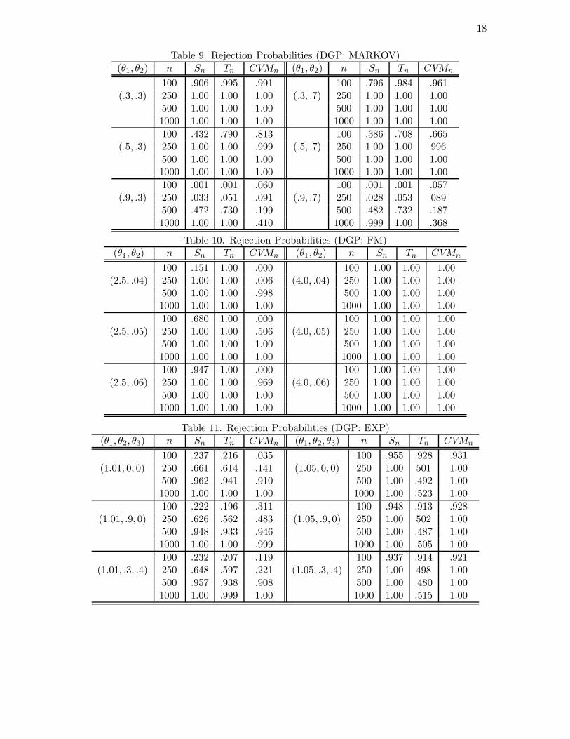
Table 8 presents the results for nonlinear moving average models. Our tests exhibitsubstantially better power performance than CVMn in relatively large samples, as the co-efficient for the linear autoregressive part θ1 gets close to unity. The results for the markovswitching models are reported in Table 9. All three tests appear to have satisfactory dis-criminatory powers against the nonmartingale markov switching models unless they havethe autoregressive coefficient θ1 close to unity. The finite sample powers of our tests Sn andTn against the nonmartingale markov switching models with the near-unity autoregressivecoefficient can be quite low, when the sample size is small. However, they increase rapidlyas the sample size increases. For the CVMn test, the rate of increase in powers with respectto sample size is much slower, as is for many other cases considered here.

Table 10 shows that our tests are consistent against the Feigenbaum map with noise.It shows that the powers increase as the process becomes chaotic (i.e., θ1 = 4) and as theprocess has more system noise (i.e., as θ2 increases). One can see that our tests performbetter than CVMn when θ1 = 2.5, while all the tests have complete distinguishing poweragainst the case θ2 = 4.

Table 11 presents the power performance against an explosive AR(1) process. Althoughthe latter process violates our Assumption 4.2, both Sn and Tn are consistent against themidly explosive alternatives (i.e., θ2 = 1.01) and more powerful than CV Mn. However, whenthe process becomes more explosive (i.e., θ2 = 1.05), Tn does not appear to be consistent.

Table 12 shows that our tests are not consistent against a unit root process with AR(1)disturbances, except the case when the AR coefficient θ1 = 1. This is expected because,even if this process satisfies E(4yt|yt−1) 6= 0 with positive probability, the correlation ofut = 4yt and yt−1 (which is nonstationary) merely shifts the limiting distributions ofour test statistics, see Section 4 for details. However, our tests do have some nontrivialpowers against this alternative process and their powers tend to increase as we have morepersistency in the innovation sequence, i.e. as θ1 gets larger.

Finally, Table 13 shows that both Sn and Tn have satisfactory power performance againsta nonstationary process with a deterministic trend. As expected, CV Mn does not have anydistinguishing power against such alternative.

16

Table 3. Rejection Probabilities (DGP: NULL)

(θ1, θ2) n Sn Tn CVMn (θ1, θ2) n Sn Tn CVMn

100 .043 .044 .033 100 .042 .047 .076(.0, .0) 250 .048 .047 .030 (.2, .3) 250 .049 .042 090

500 .028 .041 .031 500 .039 .045 .0821000 .042 .042 .035 1000 .040 .044 .095

100 .043 .050 .101 100 .039 .050 .116(.3, .0) 250 .049 .043 .114 (.3, .4) 250 .050 .041 145

500 .040 .047 .118 500 .040 .044 .1641000 .039 .049 .114 1000 .039 .038 .171

100 .032 .054 .310 100 .035 .051 .271(.9, .0) 250 .035 .049 .453 (.7, .2) 250 .043 .045 403

500 .038 .047 .535 500 .040 .051 .4831000 .043 .051 .656 1000 .043 .051 .578

Table 4. Rejection Probabilities (DGP: ARMA)

(θ1, θ2) n Sn Tn CVMn (θ1, θ2) n Sn Tn CVMn

100 .822 .989 .990 100 .457 .818 .657(.3, .0) 250 1.00 1.00. 1.00 (.3, .2) 250 1.00 1.00 1.00

500 1.00 1.00 1.00 500 1.00 1.00 1.001000 1.00 1.00 1.00 1000 1.00 1.00 1.00

100 .337 .688 .755 100 .094 .229 .160(.5, .0) 250 1.00 1.00 .998 (.5, .2) 250 .993 1.00 700

500 1.00 1.00 1.00 500 1.00 1.00 .9951000 1.00 1.00 1.00 1000 1.00 1.00 1.00

100 .000 .000 .038 100 .001 .008 .045(.95, .0) 250 .003 .001 .045 (.7, .2) 250 .530 .855 182

500 .040 .040 .067 500 1.00 1.00 .5881000 .484 .735 .103 1000 1.00 1.00 .986

Table 5. Rejection Probabilities (DGP: EXAR)(θ1, θ2) n Sn Tn CVMn (θ1, θ2) n Sn Tn CVMn

100 .010 .022 .188 100 .005 .021 .030(.6, .2) 250 .598 .905 .515 (.9, .2) 250 .020 .028 044

500 1.00 1.00 .905 500 .071 .118 .0671000 1.00 1.00 1.00 1000 .176 .177 .096

100 .001 .001 .111 100 .086 .224 .031(.6, .3) 250 .148 .308 .257 (.9, .3) 250 .185 .342 061

500 .947 1.00 .582 500 .609 .703 .1451000 1.00 1.00 .931 1000 .976 .976 .319

100 .000 .000 .070 100 .299 .474 .021(.6, .4) 250 .012 .024 .114 (.9, .4) 250 .427 .505 057

500 .307 .692 .278 500 .837 .937 .1981000 1.00 1.00 .556 1000 1.00 1.00 .536

17

Table 6. Rejection Probabilities (DGP: TAR)(θ1, θ2) n Sn Tn CVMn (θ1, θ2) n Sn Tn CVMn

100 .016 .011 .090 100 .500 .616 .655(.3, 1.0) 250 .379 .270 .166 (.3, 2.0) 250 .997 .997 948

500 .972 .950 .349 500 1.00 1.00 1.001000 1.00 1.00 .664 1000 1.00 1.00 1.00

100 .005 .004 .071 100 .151 .211 .328(.5, 1.0) 250 .207 .167 .128 (.5, 2.0) 250 .956 .957 688

500 .880 .894 .276 500 1.00 1.00 .9521000 1.00 1.00 .547 1000 1.00 1.00 1.00

100 .001 .000 .060 100 .017 .029 .118(.7, 1.0) 250 .073 .085 .102 (.7, 2.0) 250 .456 .499 249

500 .690 .810 .221 500 .990 .994 .5251000 1.00 1.00 .441 1000 1.00 1.00 .869

Table 7. Rejection Probabilities (DGP:BL)(θ1, θ2) n Sn Tn CVMn (θ1, θ2) n Sn Tn CVMn

100 .606 .908 .892 100 .001 .013 .117(.4, .1) 250 1.00 1.00 1.00 (.8, .1) 250 .361 .630 185

500 1.00 1.00 1.00 500 .997 1.00 .3921000 1.00 1.00 1.00 1000 1.00 1.00 .762

100 .563 .865 .793 100 .001 .008 .178(.4, .2) 250 1.00 1.00 .997 (.8, .2) 250 .220 .438 296

500 1.00 1.00 1.00 500 .938 .996 .5091000 1.00 1.00 1.00 1000 1.00 1.00 .818

100 .460 .758 .621 100 .001 .004 .263(.4, .3) 250 1.00 1.00 .981 (.8, .3) 250 .070 .217 566

500 1.00 1.00 1.00 500 .521 .852 .8601000 1.00 1.00 1.00 1000 .985 .999 .979

Table 8. Rejection Probabilities (DGP: NLMA)(θ1, θ2) n Sn Tn CVMn (θ1, θ2) n Sn Tn CVMn

100 .598 .914 .922 100 .005 .009 .135(.4, .2) 250 1.00 1.00 1.00 (.8, .2) 250 .410 .671 352

500 1.00 1.00 1.00 500 .999 1.00 .7101000 1.00 1.00 1.00 1000 1.00 1.00 .986

100 .596 .926 .912 100 .006 .010 .146(.4, .4) 250 1.00 1.00 1.00 (.8, .4) 250 .453 .709 349

500 1.00 1.00 1.00 500 .995 1.00 .7101000 1.00 1.00 1.00 1000 1.00 1.00 .968

100 .577 .918 .902 100 .007 .011 .168(.4, .6) 250 1.00 1.00 1.00 (.8, .6) 250 .463 .742 368

500 1.00 1.00 1.00 500 .998 1.00 .6971000 1.00 1.00 1.00 1000 1.00 1.00 .957

18

Table 9. Rejection Probabilities (DGP: MARKOV)(θ1, θ2) n Sn Tn CVMn (θ1, θ2) n Sn Tn CVMn

100 .906 .995 .991 100 .796 .984 .961(.3, .3) 250 1.00 1.00 1.00 (.3, .7) 250 1.00 1.00 1.00

500 1.00 1.00 1.00 500 1.00 1.00 1.001000 1.00 1.00 1.00 1000 1.00 1.00 1.00

100 .432 .790 .813 100 .386 .708 .665(.5, .3) 250 1.00 1.00 .999 (.5, .7) 250 1.00 1.00 996

500 1.00 1.00 1.00 500 1.00 1.00 1.001000 1.00 1.00 1.00 1000 1.00 1.00 1.00

100 .001 .001 .060 100 .001 .001 .057(.9, .3) 250 .033 .051 .091 (.9, .7) 250 .028 .053 089

500 .472 .730 .199 500 .482 .732 .1871000 1.00 1.00 .410 1000 .999 1.00 .368

Table 10. Rejection Probabilities (DGP: FM)(θ1, θ2) n Sn Tn CVMn (θ1, θ2) n Sn Tn CVMn

100 .151 1.00 .000 100 1.00 1.00 1.00(2.5, .04) 250 1.00 1.00 .006 (4.0, .04) 250 1.00 1.00 1.00

500 1.00 1.00 .998 500 1.00 1.00 1.001000 1.00 1.00 1.00 1000 1.00 1.00 1.00

100 .680 1.00 .000 100 1.00 1.00 1.00(2.5, .05) 250 1.00 1.00 .506 (4.0, .05) 250 1.00 1.00 1.00

500 1.00 1.00 1.00 500 1.00 1.00 1.001000 1.00 1.00 1.00 1000 1.00 1.00 1.00

100 .947 1.00 .000 100 1.00 1.00 1.00(2.5, .06) 250 1.00 1.00 .969 (4.0, .06) 250 1.00 1.00 1.00

500 1.00 1.00 1.00 500 1.00 1.00 1.001000 1.00 1.00 1.00 1000 1.00 1.00 1.00

Table 11. Rejection Probabilities (DGP: EXP)(θ1, θ2, θ3) n Sn Tn CVMn (θ1, θ2, θ3) n Sn Tn CVMn

100 .237 .216 .035 100 .955 .928 .931(1.01, 0, 0) 250 .661 .614 .141 (1.05, 0, 0) 250 1.00 501 1.00

500 .962 .941 .910 500 1.00 .492 1.001000 1.00 1.00 1.00 1000 1.00 .523 1.00

100 .222 .196 .311 100 .948 .913 .928(1.01, .9, 0) 250 .626 .562 .483 (1.05, .9, 0) 250 1.00 502 1.00

500 .948 .933 .946 500 1.00 .487 1.001000 1.00 1.00 .999 1000 1.00 .505 1.00

100 .232 .207 .119 100 .937 .914 .921(1.01, .3, .4) 250 .648 .597 .221 (1.05, .3, .4) 250 1.00 498 1.00

500 .957 .938 .908 500 1.00 .480 1.001000 1.00 .999 1.00 1000 1.00 .515 1.00

19

Table 12. Rejection Probabilities (DGP: UNIT)θ1 n Sn Tn CVMn θ1 n Sn Tn CVMn

100 .062 .064 .112 100 .367 .343 1.000.1 250 .059 .060 .303 0.7 250 .347 .302 1.00

500 .056 .060 .560 500 .360 .312 1.001000 .061 .059 .874 1000 .338 .302 1.00

100 .119 .113 .774 100 .647 .613 1.000.3 250 .113 .102 .998 0.9 250 .612 .572 1.00

500 .110 .099 1.00 500 .601 .568 1.001000 .109 .099 1.00 1000 .596 .560 1.00

100 .219 .206 .996 100 .900 .870 1.000.5 250 .209 .185 1.00 1.0 250 .941 .934 1.00

500 .207 .185 1.00 500 .958 .943 1.001000 .194 .177 1.00 1000 .972 .960 1.00

Table 13. Rejection Probabilities (DGP: TREND)(θ1, θ2) n Sn Tn CVMn (θ1, θ2) n Sn Tn CVMn

100 .083 .101 .037 100 .158 .164 .037(.01, .1) 250 .150 .131 .036 (.05, .1) 250 .325 .287 036

500 .249 .204 .031 500 .583 .498 .0311000 .447 .320 .036 1000 .858 .751 .036

100 .283 .229 .040 100 .443 .339 .040(.01, .3) 250 .635 .444 .039 (.05, .3) 250 .833 .668 039

500 .914 .727 .039 500 .987 .916 .0391000 .998 .957 .049 1000 1.00 .997 .049

100 .638 .419 .041 100 .754 .577 .041(.01, .5) 250 .961 .812 .048 (.05, .5) 250 .989 .922 048

500 1.00 .985 .066 500 1.00 .997 .0661000 1.00 1.00 .099 1000 1.00 1.00 .099

6. Proofs

6.1 Proof of Lemma 3.2 The stated result follows directly from Theorem 2.23 of Halland Heyde (1980), which shows that

∣

∣

∣

∣

∣

1

n

n∑

t=1

u2t −

1

n

n∑

t=1

E(u2t |Ft−1)

∣

∣

∣

∣

∣

→p 0

as n → ∞. �

6.2 Proof of Lemma 3.3 The proof for the weak convergence of Mn to M consists oftwo parts: weak convergence of finite dimensional distribution of Mn to that of M , andtightness of (Mn). To prove the first part, we let (ci) and (xi) be finite sets of numbers that

20

are given arbitrarily, and consider the transformation Π defined by

Π(f)(r) =∑

i

ci1{f(r) ≤ xi}

on D[0, 1]. It is straightforward to see that the transformation Π is continuous on C[0, 1] ⊂D[0, 1] a.s. Note that the Skorohod metric coincides with the uniform norm if restricted tothe set of continuous functions C[0, 1] defined on [0, 1]. It now follows from the continuousmapping theorem that

Π(Wn) =∑

i

ci1{Wn(·) ≤ xi}

→d Π(W ) =∑

i

ci1{W (·) ≤ xi} (20)

in D[0, 1], and therefore, we have

∑

i

ciMn(xi) =

∫ 1

0

∑

i

ci1{Wn(r) ≤ xi} dWn(r)

→d

∫ 1

0

∑

i

ci1{W (r) ≤ xi} dW (r)

=∑

i

ciM(xi) (21)

due to the result in Kurtz and Protter (1991).To establish the tightness, we show that Chentsov criterion [see, e.g., Billingsley (1968,

Theorem 15.6)] holds. Fix −∞ ≤ x < y ≤ ∞ and let w be an arbitrary number between xand y. We consider

(

Mn(x) − Mn(w))2(

Mn(w) − Mn(y))2

=1

n2

(

n∑

t=1

ut1

{

x <yt−1√

n≤ w

}

)2( n∑

t=1

ut1

{

w <yt−1√

n≤ y

}

)2

=1

n2

∑

i,j,k,`

uiujuku` 1

{

x <yi−1√

n,yj−1√

n< w

}

1

{

w <yk−1√

n,y`−1√

n< y

}

It can be easily deduced that

E(

Mn(x) − Mn(w))2(

Mn(w) − Mn(y))2

=1

n2

∑

i,j<k

Euiuju2k 1

{

x <yi−1√

n,yj−1√

n< w

}

1

{

w <yk−1√

n< y

}

+1

n2

∑

i,j<k

Euiuju2k 1

{

x <yk−1√

n< w

}

1

{

w <yi−1√

n,yj−1√

n< y

}

(22)

21

using the fact that (ut,Ft) is a martingale difference sequence and (yt) is adapted to (Ft).We will only consider the first term in (22). The treatment of the second term is entirelyanalogous. For the first term in (22), we have

1

n2

∑

i,j<k

Euiuju2k 1

{

x <yi−1√

n,yj−1√

n< w

}

1

{

w <yk−1√

n< y

}

=1

n2

n∑

j=1

E

(

j−1∑

i=1

ui1

{

x <yi−1√

n≤ w

}

)2

u2j1

{

w <yj−1√

n< y

}

=1

n2

n∑

j=1

E

(

j−1∑

i=1

ui1

{

x <yi−1√

n≤ w

}

)2

E(u2j |Fj−1)1

{

w <yj−1√

n< y

}

≤ 1

n2

E

n∑

j=1

(

j−1∑

i=1

ui1

{

x<yi−1√

n≤w

}

)4

1/2[

E

n∑

t=1

(

E(u2t |Ft−1)

)21

{

w<yt−1√

n≤y

}

]1/2

.(23)

The inequality in the last line, in particular, follows from Cauchy-Schwarz inequality.We now consider two terms appearing in (23). To analyze the first term, we may apply a

maximal inequality for martingale [see, e.g., Revuz and Yor (1994, Corollary 1.6, pp 50-51)]to get

E

max1≤j≤n

(

1√n

j∑

i=1

ui1

{

x <yi−1√

n≤ w

}

)4

≤ (4/3)4E

(

1√n

n∑

t=1

ut1

{

x <yt−1√

n≤ w

}

)4

.

(24)Moreover, it can be deduced from Rosenthal’s inequality [see, e.g., Hall and Heyde (1980,Theorem 2.12, pp 23-24)],

E

(

1√n

n∑

t=1

ut1

{

x <yt−1√

n≤ w

}

)4

≤ K

E

(

1

n

n∑

t=1

E(u2t |Ft−1)1

{

x <yt−1√

n≤ w

}

)2

+1

n2

n∑

t=1

Eu4t

(25)

for some absolute constant K. Under the condition given in Assumption 3.1(b), the secondterm in (25) is of order Op(n

−1) uniformly in w. Therefore, it will be ignored in oursubsequent derivation. We also have under Assumption 3.1(b)

supt≥1

(

E(

u2t

∣

∣

∣Ft−1

))2≤ sup

t≥1E(

u4t

∣

∣

∣Ft−1

)

< K a.s. (26)

due to the conditional Jensen’s inequality. Consequently,

supt≥1

E(

u2t

∣

∣

∣Ft−1

)

< K1/2 a.s.

22

Therefore, it follows from (24) and (25) that

E

1

n

n∑

j=1

(

1√n

j−1∑

i=1

ui1

{

x <yi−1√

n≤ w

}

)4

≤ K

E

(

1

n

n∑

t=1

1

{

x <yt−1√

n≤ w

}

)2

(27)

for some constant K. To deal with the second term in (23), we use (26) to deduce that

E

[

1

n

n∑

t=1

(E(u2t |Ft−1))

21

{

w <yt−1√

n≤ y

}

]

≤ K

[

E

(

1

n

n∑

t=1

1

{

w <yt−1√

n≤ y

}

)]

(28)

for some constant K.Let k = 1, 2. For any fixed x and y, we have

(

1

n

n∑

t=1

1

{

x <yt−1√

n≤ y

}

)k

=

(∫ 1

01{x < Wn(r) ≤ y} dr

)k

→d

(∫ 1

01{x < W (r) ≤ y} dr

)k

which holds as a special case of (20). However, since

(

1

n

n∑

t=1

1

{

x <yt−1√

n≤ y

}

)k

≤ 1

and bounded, we have

E

(

1

n

n∑

t=1

1

{

x <yt−1√

n≤ y

}

)k

→ E

(∫ 1

01{x < W (r) ≤ y} dr

)k

(29)

as n → ∞.By the occupation times formula, we have

∫ 1

01{x < W (r) ≤ y} dr =

∫ ∞

−∞1{x < s ≤ y}L(1, s) ds

where L is the local time of the standard Brownian motion. Therefore, it follows that

E

(∫ 1

01{x < W (r) ≤ y} dr

)k

= E

(∫ y

xL(1, s) ds

)k

= (y − x)kE

(

1

y − x

∫ y

xL(1, s) ds

)k

≤ (y − x)kE

(

1

y − x

∫ y

xL(1, s)kds

)

≤ (y − x)k sups∈R

EL(1, s)k, (30)

23

where the last inequality is due to Fubini’s theorem.Let a and b be constants such that

P

{

a ≤ min0≤r≤1

W (r), max0≤r≤1

W (r) ≤ b

}

> 1 − ε

for ε > 0 arbitrarily small. For x, y ∈ [a, b], we now have from (22), (23), (27), (28), (29)and (30) that

E(

Mn(x) − Mn(w))2(

Mn(w) − Mn(y))2

≤ K(w − x)(y − w)1/2

≤ K(y − x)3/2 (31)

for some constant K. This establishes Chenstov condition for tightness. The tightnessresult in (31), together with the weak convergence of the finite dimensional distributionsshown in (21), proves the stated result. �

6.3 Proof of Theorem 3.4 The stated results follow directly from the continuous map-ping theorem, given the weak convergence of Mn to M that is established in Lemma 3.3.�

6.4 Proof of Lemma 3.5 Let x < y, and note that

|M(x) − M(y)|p =

∣

∣

∣

∣

∫ 1

01{W (r) ≤ x} dW (r) −

∫ 1

01{W (r) ≤ y} dW (r)

∣

∣

∣

∣

p

=

∣

∣

∣

∣

∫ 1

01{x < W (r) ≤ y} dW (r)

∣

∣

∣

∣

p

.

We have

E

∣

∣

∣

∣

∫ 1

01{x < W (r) ≤ y} dW (r)

∣

∣

∣

∣

p

≤ cE

∣

∣

∣

∣

∫ 1

01{x < W (r) ≤ y} dr

∣

∣

∣

∣

p/2

for some constant c, as shown in, e.g., Revuz and Yor (1994, Proposition 4.3, p154), and∫ 1

01{x < W (r) ≤ y} dt =

∫ ∞

−∞1{x < s ≤ y}L(1, s) ds

= |x − y| sups∈R

L(1, s).

Consequently, it follows that

E|M(x) − M(y)|p ≤ c |x − y|p/2E

(

sups∈R

L(1, s)

)p/2

and we may simply let

cp = cE

(

sups∈R

L(1, s)

)p/2

to get the stated result. �

24

6.5 Proof of Proposition 3.6 The result follows from Lemma 3.5. See, for instance,Revuz and Yor (1994, Theorem 2.1, p. 25). �

6.6 Proof of Lemma 4.3 Let Fnt(·) denote the distribution function of ynt. For aninteger K > 1, let

ξntm = inf{

x ∈ R :Fnt(x) ≥ m

K

}

for m = 1, ...,K − 1,

and also let ξnt0 = −∞ and ξntK = +∞. Define F = {4ynt1{yn,t−1 ≤ x} : x ∈ R} tobe a class of functions and we denote a uniform analogue of the L1- norm by ρ(f) =supn,t E|f(xnt)| for f ∈ F , where xnt = (ynt, yn,t−1)

′.By construction, for each x ∈ R, there exists m ∈ {1, ...,K − 1} such that

|Fnt(x) − Fnt(ξntm)| ≤ 1

K,

so that

|4ynt [1{yn,t−1 ≤ x} − 1{yn,t−1 ≤ ξntm}]|≤ |4ynt| sup

y:|Fnt(y)−Fnt(ξntm)|≤ 1

K

|1{yn,t−1 ≤ y} − 1{yn,t−1 ≤ ξntm}|

≡ bntm, say. (32)

This result implies that for any function 4ynt1{yn,t−1 ≤ x} in F , there exists m ∈ {1, ...,K−1} such that

lm ≤ 4ynt1{yn,t−1 ≤ x} ≤ um ,

where

lm = 1{yn,t−1 ≤ ξntm} − bntm,

um = 1{yn,t−1 ≤ ξntm} + bntm.

Note that we have

ρ(bntm) = supn,t

E |4ynt| supy:|Fnt(y)−Fnt(ξntm)|≤ 1

K

|1{yn,t−1 ≤ y} − 1{yn,t−1 ≤ ξntm}|

≤ supn,t

E |4ynt| 1{ξnt,m−1 ≤ yn,t−1 ≤ ξnt,m+1}

≤ supn,t

(E|4ynt|p)1/p supn,t

|Fnt(ξnt,m+1) − Fnt(ξnt,m−1)|1−1/p

= C1

(

1

K

)1−1/p

, (33)

where C1 = 21−1/p supn,t E|4ynt|p < ∞ by Assumption 4.2 and the second inequality holdsby Holder’s inequality. Therefore,

{[lm, um] : m = 1, ...,K − 1}}

25

forms an ε = 2C1K1/p−1 bracket for (F , ρ) . Hence, the bracketing number (see, e.g., van

der Vaart and Wellner (1996, p.83) for the definition) satisfies

N(ε,F , ρ) ≤(

2C1

ε

)p/(p−1)

< ∞. (34)

This result and pointwise WLLN of Andrews (1988, example 4, p.462) give the desired resultusing an argument similar to Lemma 2.4.1 of van der Vaart and Wellner (1996, p.123). �

6.7 Proof of Theorem 4.4 Under Assumption 4.2, we have

σn →p

(

limn→∞

1

n

n∑

t=1

E (4ynt)2

)1/2

≡ σ∗ < ∞ (35)

by WLLN of Andrews (1988, example 4, p.462). Define

Q(y) =

∫

H(z)1(z ≤ y) dP(z). (36)

Then, by Lemma 4.3, (35) and rearranging terms, we have

n−1/2Sn →p (1/σ∗) supy∈R

|Q(y)| (37)

and

n−1Tn →p (1/σ∗)

∫

Q2(y) dP(y). (38)

The stated result now follows since the right hand sides of (37) and (38) are positive underAssumption 4.1. �

References

An, H.-Z. and C. Bing (1991). “A Kolmogorov-Smirnov type statistic with application totest for nonlinearity in time series,” International Statistical Review, 59, 287-307.

Andrews, D. W. K. (1988). ”Laws of large numbers for dependent non-identically dis-tributed random variables,” Econometric Theory, 4, 458-467.

Andrews, D. W. K. (1994). “Empirical process methods in econometrics,” In R.F. Engleand D. McFadden, eds., Handbook of Econometrics, Vol.4, Elsevier: Amsterdam.

Andrews, D. W. K. (1997). ”A conditional Kolmogorov test,” Econometrica, 65, 1097-1128.

Billingsley, P. (1968). Convergence of Probability Measures. John Wiley: New York.

26

Billingsley, P. (1995). Probability and Measure, 3rd ed. John Wiley: New York.

Bierens, H.J. (1990). “A consistent conditional moment test of functional form,” Econo-

metrica, 58, 1443-1458.

Bierens, H.J. and W. Ploberger (1997). “Asymptotic theory of integrated conditionalmoment tests,” Econometrica, 65, 1129-1152.

Brockett, P.L., M. Hinich, and D. Patterson (1988). “Bispectral based tests for the detec-tion of Gaussianity and linearity in time series,” Journal of the American Statistical

Association, 83, 657-664.

Chan, W.S. and H. Tong (1986). “On tests for non-linearity in time series analysis,”Journal of Forecasting, 5, 217-228.

Chang, Y. and J.Y. Park (2004). “Endogeneity in nonlinear regressions with integratedtime series,” unpublished manuscript, Department of Economics, Rice University.

Chung, K.L. and R.T. Williams (1990). Introduction to Stochastic Integration. Birkhauser:Boston.

de Jong, R. M. (1995). ”Law of large numbers for dependent heterogeneous processes,”Econometric Theory, 11, 347-358.

de Jong, R. M. (1996). “The Bierens test under data dependence,” Journal of Economet-

rics, 72, 1-32.

Delgado, M. (1993). ”Testing the equality of nonparametric regression curves,” Statistics

and Probability Letters, 17, 199-204.

Deo, R. S. (2000). ”Spectral tests of the martingale hypothesis under conditional het-eroscedasticity,” Journal of Econometrics, 99, 291-315.

Dickey, D. A. and W. A. Fuller (1979). “Distribution of estimators for autoregressive timeseries with a unit root,” Journal of the American Statistical Association, 74, 427-431.

Dominguez, M. A. and I. N. Lobato (2000). ”A consistent test for the martingale differencehypothesis,” unpublished manuscript, Instituto Tecnologico Autonomo de Mexico.

Durlauf, S.N. (1991). “Spectral based testing of the martingale hypothesis,” Journal of

Econometrics, 50, 355-376.

Enders, W. and C. W. J. Granger (1998). “Unit root tests and asymmetric adjustmentwith an example using the term structure of interest rates,” Journal of Business and

Economic Statistics, 16, 304-311.

Hall, R. E. (1978). “Stochastic implications of the life cycle-permanent income hypothesis:Theory and evidence,” Journal of Polical Economy, 86, 971-987.

27

Hall, P. and C.C. Heyde (1980). Martingale Limit Theory and Its Application. AcademicPress: New York.

Hida, T. (1980). Brownian Motion. Springer-Verlag: New York.

Hinich, M. (1982). “Testing for Gaussianity and linearity of a stationary time series,”Journal of Time Series Analysis, 3, 169-176.

Hjellvik, V. and D. Tjøstheim (1995). “Nonparametric tests of linearity for time series,”Biometrika, 82, 351-368.

Hong, Y. (1999). ”Hypothesis testing in time series via the empirical characteristic func-tion: A generalized spectral density approach,” Journal of the American Statistical

Association, 84, 1201-1220.

Khmaladze, E. V. (1988), ”An innovation approach to goodness-of-fit tests in Rm, ” Annals

of Statistics, 16, 1503-1516.

Koul, H. and W. Stute (1999), ”Nonparametric model checks for time series,” Annals of

Statistics, 27, 204-236.

Kuan, C. -M. and W. -M. Lee (2003), ”A new test of the martingale difference hypothesis,”unpublished manuscript, Institute of Economics, Academia Sinica.

Kurtz, T.G. and P. Protter (1991). “Weak limit theorems for stochastic integrals andstochastic differential equations,” Annals of Probability, 19, 1035-1070.

Luukkonen, R., P. Saikkonen, and T. Terasvirta (1988). “Testing linearity against smoothtransition autoregression,” Biometrika, 75, 491-499.

Phillips, P. C. B. (1997). “Unit root tests.” In Encyclopedia of Statistical Sciences Vol.12, Wiley: New York.

Park, J.Y. and P.C.B. Phillips (1999). “Asymptotics for nonlinear transformations ofintegrated time series,” Econometric Theory, 15, 269-298.

Revuz, D. and M. Yor (1994). Continuous Martingale and Brownian Motion, 2nd ed.Springer–Verlag: New York.

Shorack, G. R. and J. A. Wellner (1986). Empirical Processes with Applications to Statis-

tics, Wiley: New York.

Stinchcombe, M. B. and H. White (1998). ”Consistent specification testing with nuisanceparameters present only under the alternative,” Econometric Theory 14, 295-325.

Stock, J.H. (1994). “Unit roots and structural breaks,” In R.F. Engle and D. McFadden,eds., Handbook of Econometrics, Vol. 4, 2739-2841, Elsevier: Amsterdam.

Stute, W. (1997). ”Nonparametric model checks for regression,” Annals of Statistics, 25,613-641.

28

Tong, H. (1990). Nonlinear Time Series: A Dynamical Systems Approach. ClarendonPress: Oxford.

van der Vaart, A. W. and Wellner, J. A. (1996). Weak Convergence and Empirical Pro-

cesses. Springer-Verlag: New York.

Whang, Y. -J. (2000). ”Consistent bootstrap tests of parametric regression functions,”Journal of Econometrics, 98, 27-46.

Whang, Y. -J. and O. Linton (1999). “The asymptotic distribution of nonparametric esti-mates of the Lyapunov exponent for stochastic time series,” Journal of Econometrics,91, 1-42.

29