a theoretical analysis of camera response …jye/lab_research/eccv/eccv12-crf.pdfa theoretical...

A Theoretical Analysis of Camera ResponseFunctions in Image Deblurring

Xiaogang Chen1,2,3, Feng Li3, Jie Yang1,2, and Jingyi Yu3

1 Shanghai Jiao Tong University, Shanghai, China.2 Key Laboratory of System Control and Information Processing,

Ministry of Education, Shanghai, China. {cxg,jieyang}@sjtu.edu.cn3 University of Delaware, Newark, DE, USA. {feli,yu}@cis.udel.edu

Abstract. Motion deblurring is a long standing problem in computervision and image processing. In most previous approaches, the blurredimage is modeled as the convolution of a latent intensity image with ablur kernel. However, for images captured by a real camera, the blurconvolution should be applied to scene irradiance instead of image inten-sity and the blurred results need to be mapped back to image intensityvia the camera’s response function (CRF). In this paper, we present acomprehensive study to analyze the effects of CRFs on motion deblur-ring. We prove that the intensity-based model closely approximates theirradiance model at low frequency regions. However, at high frequen-cy regions such as edges, the intensity-based approximation introduceslarge errors and directly applying deconvolution on the intensity imagewill produce strong ringing artifacts even if the blur kernel is invertible.Based on the approximation error analysis, we further develop a dual-image based solution that captures a pair of sharp/blurred images forboth CRF estimation and motion deblurring. Experiments on syntheticand real images validate our theories and demonstrate the robustnessand accuracy of our approach.

1 Introduction

Image deblurring is a long standing problem in computer vision and image pro-cessing. A common assumption in most existing approaches is that a blurredimage is the convolution result of a blur-free intensity image I with a blur ker-nel K, i.e., B = I ⊗K. However, for images captured by a real camera, the blurconvolution should be applied to image irradiance I rather than image intensity.The blurred results then need to be mapped back to image intensity via thecamera’s response function (CRF) ψ as:

B = ψ(I ⊗K). (1)

Eqn. (1) reveals that, unless the CRF ψ is linear, the actual captured blur image

B will be different from the synthetically blurred intensity image B. The correctway to deblur B hence is to first map B back to irradiance as ψ−1(B), then

2 Xiaogang Chen, Feng Li, Jie Yang, and Jingyi Yu

apply deconvolution, and finally map it back to intensity. In reality, recoveringthe CRF ψ of a real camera often requires applying complex calibration processes[1] or using special scene settings [2].

Previously irradiance domain deconvolution methods assume a known CR-F curve [3, 4]. More recently approaches [5–8] apply additional constraints inthe intensity domain to reduce visual artifacts. Although they simplify the es-timation, they may introduce significant approximation errors caused by theunderlying linear CRF assumption. More important, it is desirable to character-ize how close the intensity based convolution is to the ground truth irradianceblurring model and where the errors are large.

In this paper, we present a comprehensive study to analyze the effect of CRFson motion deblurring. Our contributions are two-folded. On the theory side, weprove that the intensity-based blur model closely approximates the irradiance-based one at low frequency regions. We further derive a closed-form error boundto quantitatively measure the difference between B and B. However, at highfrequency regions such as near texture or occlusion edges, the intensity-basedapproximation introduces large errors and directly applying deconvolution on theintensity image introduces ringing artifacts even if the blur kernel is invertible.

On the application front, we develop a simple but effective computationalphotography technique to recover the CRF. Our approach is inspired by therecent single-image based CRF estimation method [9] that strategically blursthe image under 1D linear motion. We, instead, capture a pair of sharp/blurredimages and directly use motion blurs caused by hand shakes. Specifically, we firstautomatically align the two images and then use the sparsity prior to recoveringthe blur kernel. To recover the CRF, we represent it using the Generalized Gam-ma Curve Model (GGCM) and find the optimal one by fitting pixels near edgeregions in the two images. Experiments on synthetic and real images validate ourtheories and demonstrate that our dual-image approach is robust and accurate.

Concurrent with this research, Kim et al. [10] independently developed asimilar analysis to characterize nonlinear CRFs in motion blur and proposed asingle-image deblurring scheme. We, on the other side, focus on the theoreticalanalysis of the approximation errors and derive an error bound.

2 Related Work

Our work is related to a number of areas in image processing and computationalimaging.

CRF Estimation. The CRF can be estimated by capturing multiple im-ages from the same viewpoint with different but known exposure settings. Thepioneer work by Debevec and Malik [1] assume smooth CRFs and form an over-determined linear system for simultaneously estimating the irradiance at eachpixel as well as the inverse CRF. Later approaches [11–14] adopt more complexCRF models based on polynomial fitting [13] or Empirical Model of Response(EMoR) [12]. EMoR, for example, is particularly useful for its low dimensional-ity and high accuracy and has been widely used in various imaging applications

A Theoretical Analysis of CRF in Image Deblurring 3

[11, 15–18]. Lee et al. [14] employed this low-rank structure of irradiance where-as Kim and Pollefeys [11] developed a full radiometric calibration algorithmto simultaneously estimate CRF, exposure, and vignetting. More recently [15],they used an outdoor image sequence with varying illumination based CRF es-timating method, while different from previous constant illumination methods[1, 12].

A downside of multi-image approaches is that both the scene and camerahave to be static during capturing. To resolve this issue, a number of single-image based approaches have been recently proposed. The classical approachuses the Macbeth color chart [2] and assumes known surface reflectance forcalibrating the radiometric function. In Lin and Zhang [17] and Lin et al. [16],the authors analyzed the linear blending properties of edges in gray scale or colorimages. Matsushita and Lin [18] explored how symmetric distribution of noisegets skewed by the CRF and used a single noisy image for recovering the CRF.Wilburn et al. [9] further analyzed how the CRF affects linearly motion blurrededges and then used the blurred edges for sampling the CRF. Their approachrequires strategically introducing a linear motion blur whereas we use generalmotion blurs, e.g., the ones caused by hand shakes.

Image Deblurring. Our work aims to actively use image blurs for recoveringthe CRF, and also analyzes ringing effect in deblurred images caused by thenonlinearity introduced by the CRF. The literature on image deblurring is hugeand we refer the readers to the recent papers [19, 20] for a thorough review. Mostexisting approaches assume that the CRF is known or linear and directly applythe deblurring on the intensity domain. More recent approaches have focusedon imposing priors to the kernel or to image statistics to improve quality. Forexample, Fergus et al. [3] assumed the gradient distribution of a sharp image isheavy-tailed and apply inference to recover the optimally deblurred result. Shanet al. [5] concatenated two piece-wise continuous functions to fit the heavy-taileddistribution and use local image constraint and high-order noise distribution tosuppress the ringing artifacts. Other types of priors such as edge sharpness [21,6], transparency [22], kernel sparsity [23] and Fields of Experts [24] have shownpromising results for image restoration. Levin et al. [19] analyzed and evaluatedmany recent blind deconvolution algorithms. Due to the complexity of bothestimating CRF and blind deconvolution, recent approaches [7, 6, 5] attemptto model the blur on image intensities by bypassing the irradiance-intensityconversion. Additional constraints such as minimal ringing can be added to thedeconvolution process. However, the underlying approximation error has beenbarely discussed.

3 Deblurring: Irradiance vs. Intensity

We first study the role of the CRF in image blurring/deblurring. Before pro-ceeding, we clarify our notation. I represents the blur-free intensity image, Erepresents its corresponding scene irradiance, ∆tI is the exposure time. We alsoassume that the CRF ψ is monotonically increasing and use ϕ to represent its


inverse. We have I = ψ(E ·∆tI) or,

E = ϕ(I)/∆tI . (2)

We use B to represent the ground truth blurred image that is obtained byfirst convolving the irradiance image E with the blur kernelK and then mappingthe result onto intensity as:

B = ψ((E ⊗K) ·∆tB), (3)

where all kernel elements in K are non-negative and sum to one. SubstitutingEqn.(2) into (3), we have:

B = ψ((ϕ(I)⊗K) · r), r = ∆tB/∆tI . (4)

r represents exposure ratio. It is important to note that Eqn. (4) simplifies theexposure ratio r in terms of the exposure time. In practice, we can factor otherexposure parameters such as the ISO and the aperture size (F number) into r 4.

In our analysis, we assume that the hypothetic latent image I and the cap-tured blurred image B have identical exposure, i.e., r = 1, and we have:

B = ψ(ϕ(I)⊗K). (5)

Actually, two images have the same exposure do not necessitate the same ex-posure settings of a camera. They may differ in exposure time, ISO value oraperture size 4.

For blind image deconvolution, the goal is to recover the latent sharp imageand the kernel. By Eqn. (5), it is straightforward to map B back to the irradi-ance domain and then perform the deconvolution. However, it is also popular touse the intensity based convolution model B = I⊗K in conventional deblurringalgorithms [5, 7]. By using additional edge prediction [6] or gradient regulariza-tion [7], the intensity based model is also able to produce pleasing deblurring

results. We aim to measure the Blur Inconsistency Γ = B−B, and to understandwhere the intensity based convolution model introduces approximation error.

3.1 Blur Inconsistency

We first study where Blur Inconsistency occurs.Claim 1. In uniform intensity regions, Γ = 0 .

Since pixels within the blur kernel region have uniform intensity, we have ϕ(I ⊗K) = ϕ(I) = ϕ(I)⊗K. Therefore,

B = ψ(ϕ(I)⊗K) = ψ(ϕ(I ⊗K)) = B,

4 As shown in [4] and [13], the exposure ratio can be calculated by r = ISOB∆tBFI2

ISOI∆tIFB2 .

ISOI and FI denote the camera ISO setting and aperture F-number relating toimage I. ISOB and FB are the corresponding values with respect to image B.


thus Γ = 0.Claim 1 applies to any (non-linear) CRF. This also implies that uniform

regions in B will not be useful to recover the CRF.Claim 2. If the blur kernel K is small and the CRF ψ is smooth, Γ ≈ 0 in

low frequency regions in I .

Proof. Let I = I + ∆I in a local patch covered by the blur kernel K. I isthe average intensity within the patch and ∆I is the deviation from I. In lowfrequency regions, ∆I is small.

Next we apply the first-order Taylor expansion to ϕ(I)⊗K as:

ϕ(I +∆I)⊗K ≈ ϕ(I)⊗K + (ϕ′(I) ·∆I)⊗K (6)

Since I is uniform, we have ϕ(I)⊗K = ϕ(I), and ϕ′(I) is constant in the localneighborhood. The right hand side (RHS) of Eqn.(6) thus can be approximatedas:

ϕ(I) + ϕ′(I) ·∆I ⊗K. (7)

Furthermore, since ϕ(I ⊗K) = ϕ(I ⊗K +∆I ⊗K), by using the first-orderTaylor expansion, we have

ϕ(I ⊗K) ≈ ϕ(I ⊗K) + ϕ′(I ⊗K) · (∆I ⊗K). (8)

Since I is constant in the local patch, the RHS of (8) is equal to:

ϕ(I) + ϕ′(I) ·∆I ⊗K. (9)

Therefore,B = ψ(ϕ(I)⊗K) ≈ ψ(ϕ(I ⊗K)) = B, (10)

i.e., Γ ≈ 0.

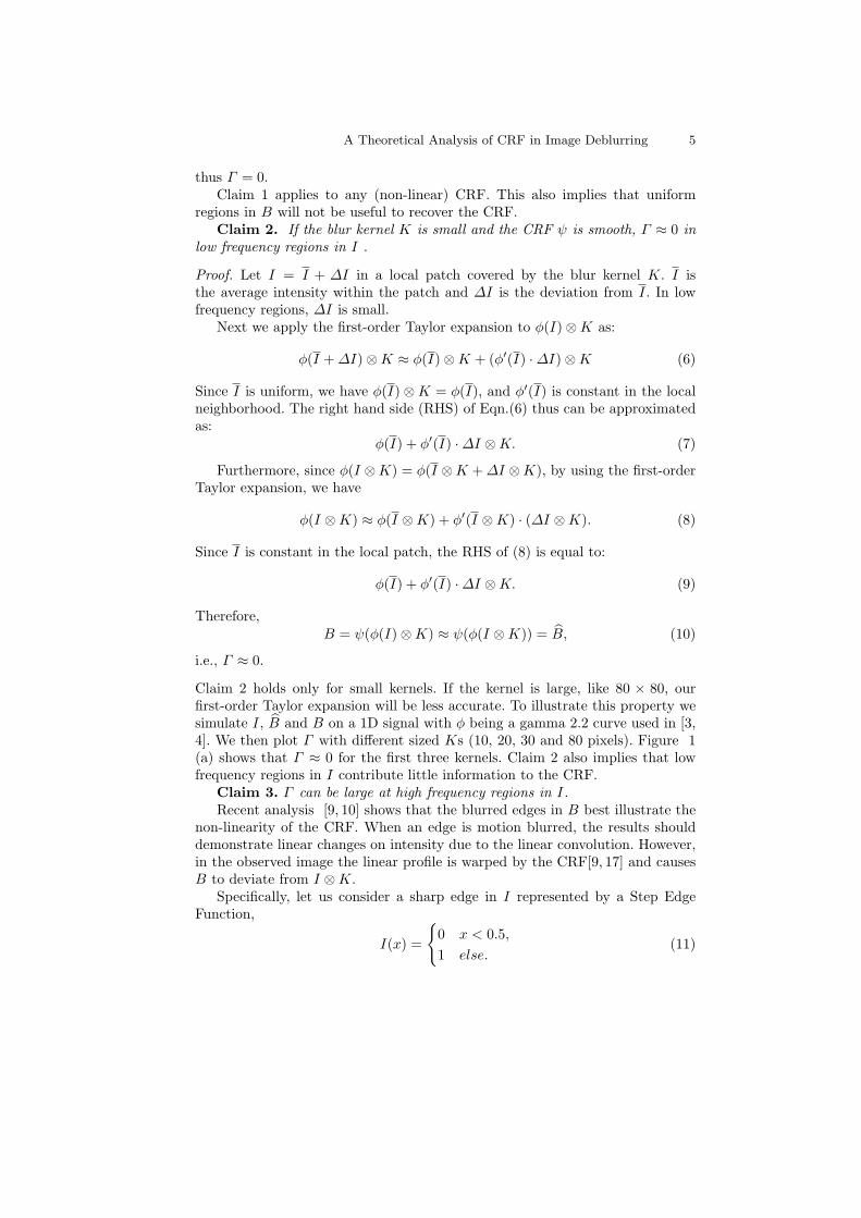
Claim 2 holds only for small kernels. If the kernel is large, like 80 × 80, ourfirst-order Taylor expansion will be less accurate. To illustrate this property wesimulate I, B and B on a 1D signal with ϕ being a gamma 2.2 curve used in [3,4]. We then plot Γ with different sized Ks (10, 20, 30 and 80 pixels). Figure 1(a) shows that Γ ≈ 0 for the first three kernels. Claim 2 also implies that lowfrequency regions in I contribute little information to the CRF.

Claim 3. Γ can be large at high frequency regions in I.Recent analysis [9, 10] shows that the blurred edges in B best illustrate the

non-linearity of the CRF. When an edge is motion blurred, the results shoulddemonstrate linear changes on intensity due to the linear convolution. However,in the observed image the linear profile is warped by the CRF[9, 17] and causesB to deviate from I ⊗K.

Specifically, let us consider a sharp edge in I represented by a Step EdgeFunction,

I(x) =

{0 x < 0.5,

1 else.(11)


0 100 200 300 400 500−0.05

0

0.05

0.1

0.15

0.2

0.25

0.3

0.35

0.4

sharp signal I

Γ(length=10)

Γ(length=20)

Γ(length=30)

Γ(length=80)

(a) (b) (c)0 50 100 150 200 250 300

-0.05

0

0.05

0.1

0.15

0.2

0.25

0.3

0.35

sharp signal IΓ(length=10)Γ(length=20)Γ(length=30)Γ(length=80)

Fig. 1. Blur Inconsistency Γ . (a): Γ is computed on a 1D sharp signal with a gamma2.2 CRF curve with four different blur kernels of size 10, 20, 30 and 80 pixels. (b):The diagram of Γ vs. different kernel sizes. Blurs are applied to the top row pattern in(c). Notice that large Γ values match sharper edges. (c): The top two rows show thelatent pattern I and the irradiance-based blurred result B. The bottom row shows themeasured Γ which varies across edge strength.

Since ϕ has boundary ϕ(0) = 0 and ϕ(1) = 1 [12], we have ϕ(I) = I. Therefore,

B = ψ(ϕ(I)⊗K) = ψ(I ⊗K) = ψ(B), (12)

and then, Γ = ψ(B) − B. In this toy example, Γ (x) simply measures the mag-nitude how ψ(x) deviates from the linear function y(x) = x. In other words,Γ (x) → 0, iff ψ(x) → x. However, practical CRFs ψ are highly nonlinear [12].

To validate Claim 3, we synthesize the blurred edges and measure their Γshown in Figure 1(c). The top row shows a sharp pattern corresponding to I.Notice that the foreground blocks gradually become brighter from left to rightand the rightmost edge has the largest scale of the step-edge. The second rowshows its corresponding horizontally motion blurred result B. ϕ is simulated byGamma 2.2. The motion length is 20 pixels. The bottom row presents Γ andclearly shows that the blurred edge regions Γ have significant deviations thatcannot be ignored. We also notice that a sharper edge leads to a larger Γ . Figure1(b) shows the horizontal profile of the Γ used in Figure 1(c). We experiment onfour different kernel sizes and show the corresponding Γ s. The results illustratethat the magnitude of Γ is closely related with the contrast of the edge whereasthe kernel size only affects the shape of Γ curve.

Finally, we analyze the more general case and provide upper and lower boundto Γ :

Theorem 1. Let Imin and Imax be the local lowest and highest pixel intensi-ties in a local neighborhood covered by kernel K in image I. If ϕ is convex, thenthe Blur Inconsistency is bounded by 0 ≤ Γ ≤ Imax − Imin.

Proof. Consider that ϕ(I)⊗K can be viewed as a convex combination of pixelsfrom ϕ(I). If ϕ is convex, we can use Jensen’s inequality and get

ϕ(I)⊗K ≥ ϕ(I ⊗K). (13)

Further, since the CRF ψ is a monotonically increasing [1, 13], we have:

B = ψ(ϕ(I)⊗K) ≥ ψ(ϕ(I ⊗K)) = B, (14)


0 0.15 0.3 0.45 0.6 0.75 0.90

0.15

0.3

0.45

0.6

0.75

0.9

irradiance

intensity

(a) (b)

Fig. 2. The left panel shows 188 CRF curves of real cameras from DoRF [12]. Nearlyall curves appear concave. For a clearer illustration, the second-order derivatives atsample points on the curves are plotted on the right. Each row corresponds to a CRFcurve where which negative derivatives are drawn in gray and positive in black.

i.e., Γ ≥ 0.Next, we derive the upper bound of Γ . Since I ⊗ K ≤ Imax and ϕ is the

inversion of ψ, it must also be monotonically increasing. Therefore ϕ(I)⊗K ≤ϕ(Imax) and we have,

B = ψ(ϕ(I)⊗K) ≤ ψ(ϕ(Imax)) = Imax. (15)

Likewise, we can also derive taht B = I ⊗ K ≥ Imin. Combining it with Eqn.(14) and Eqn. (15), we have: Imin ≤ B ≤ B ≤ Imax. Therefore,

0 ≤ Γ ≤ Imax − B ≤ Imax − Imin. (16)

Theorem 1 explains the phenomenon in Figure 1 (b) and (c): when theintensity contrast (gradient) of an edge is high, the upper-bound of Γ will belarge. In contrast, in low-frequency regions, the upper bound Imax−Imin is lowerand so is Γ , i.e., B can be well approximated by B.

It is important to note that Theorem 1 assumes a convex inverse CRF ϕ.This property has been observed in many previous results. For example, thewidely used Gamma curves ϕ(x) = xγ , γ > 1, are convex. To better illustratethe convexity of ϕ or equally the concavity of ψ, we plot in Figure 2 188 realcamera CRF curves (ψ) collected in [12]. We represent all curves by a matrixwith 188 rows and compute the discrete second-order derivatives and show theresults in the right panel of Figure 2. The negative second-order derivatives areillustrated in gray pixels and the positive ones in black pixels. Our experimentshows that the majority (84.4%) of sample points are negative and therefore theinverse CRF ϕ is largely convex.

3.2 Deconvolution Artifacts

Our theory reveals that if a camera has a non-linear CRF, the conventionalintensity-based blur model is largely valid on uniform and smooth regions butfails near high frequency regions such as near occlusion or texture edges. Next,


⊗1

K−

1B K

−⊗B

++

P

B ⊗1

K−

Fig. 3. The ringing artifacts when deblurring a blurred step-edge function. The kernelis invertible and therefore the artifacts are caused by Γ .

we analyze the deblurring artifacts when applying brute-force intensity-baseddeblurring method.

In the first example, we analyze the 1D step-edge signal (11) for its simplicity.

By 12, we have B = ψ(B). Assume ψ is a Gamma function ψ(x) = xγ , γ < 1,we can then expand B with Taylor expansion:

B = Bγ = B + P, (17)

where P =∞∑t=1

(γ−1)t

t! B(ln B)t. An important property of function x(lnx)

tis

that it approaches zero for x → 0+ or x → 1. Therefore, P only has non-zerovalues in the blurred edge regions.

Given an invertible filter which has non-zero points in the frequency, we canrepresent the deconvolution of B with K by B ⊗K−1, and thus

B ⊗K−1 = B ⊗K−1 + P ⊗K−1, (18)

where B ⊗K−1 = I since K is invertible. P ⊗K−1 can be viewed as the decon-volution artifacts introduced by the Blur Inconsistency Γ . Figure 3 illustratesthe decomposition of (18) in details.

The ringing artifacts in the step-edge function discussed above can also beobserved in the frequency domain. Let I∗ = B⊗K−1. We assume that the fouri-er coefficient of K at a specific frequency ωn is an. Therefore, the correspondingcoefficient of K−1 at frequency ωn is 1/an. Since I is a Step Function, its co-efficient at ωn is α/n for n = 0, where α is a constant value for all n. We can

further verify that the coefficient of I ⊗K at frequency ωn is α/n · an.If ψ is a linear function, the coefficient of I∗ at frequency ωn will be β ·

α/n · an · 1/an = αβ/n where β is a constant scaling factor introduced by ψ.

Therefore, the spectrum of I∗ will be a scaled version of I, i.e., I∗ will still be astep function and there will be no ringing artifacts.

In contrast, if ψ is monotonically increasing and concave, Farid [25] provedby using Taylor’s series that the coefficients at frequency ωn for I∗ will be scalednon-linearly and non-uniformly, i.e., it will no longer be a scaled version of α/n·anand convolving it with K−1 will not cancel out an. As a result, I∗ will no longerbe a step function (edge) but a signal corrupted by non-uniformly scaled highfrequencies. Visually it will exhibit strong ringing artifacts.

Finally, we analyze and illustrate the visual artifacts caused by a non-linearCRF in image deblurring. In Figure 4, we synthesize a motion-blurred image


(a) (c) (e)

(b) (d) (f)

Fig. 4. TV-based deblurring results on the irradiance-based blur image B and on theintensity-based blur image B. (a) shows the latent intensity image I. (b) shows B (left)

and B (right). (c) and (d) show the deblurred results using TV on B and B with thesame blur kernel. (e) and (f) show the corresponding error maps.

using an invertible blur kernel under a Gamma 2.2 CRF. Figure 4(a) shows thelatent image I and the kernel K. (b) shows the irradiance-based blur image B

and the intensity-based blur image B. We apply non-blind deconvolution usingTotal Variation regularization [26] to recover the latent images from B and Brespectively. The results are shown in Figure 4 (c) and (d). Figure 4 (e) and (f)show the error map to the ground truth.

As shown in Figure 4, the TV-based technique produces high quality resultgiven B. However, applying the same deconvolutoin technique on B using thesame blur kernel produces ringing artifacts surrounding image edges. Such re-sult is consistent with our Theorem 1. Note that the edges with large contrastImax−Imin will have large Blur Inconsistency Γ , and exhibit noticeable ringingsartifacts.

Theorem 1 reveals the importance of image regularization in intensity-baseddeblurring. When images have moderate edge contrasts, our experiments showthat Total Variation regularized nonblind deconvolution can produce reasonableresults. However, for images with large edge contrasts, the Blur Inconsistency willbe large and suppressing the ringing artifacts can be difficult. The deconvolutionmodels used [5, 7] further help to suppress ringing by assuming heavy-taileddistribution, local gradient constraint, noise distribution, etc.

4 Dual-Image CRF Estimation

Based on our analysis, we present a new computational photography technique toestimate the CRF using a pair of images. Our work is inspired by the recent dual-


image processing techniques where a pair of images captured towards the samescene but under different aperture/shutter settings are used [4]. In a similar vein,we use a blurry/sharp image pair: the first image is captured with a slow shutterand introduces motion blurs whereas the second is captured with fast shutterbut high ISO. The main difference is that [4] uses known CRF for deblurringwhereas our goal is to estimate CRF from the image pair.

Recall that our analysis shows that the blurred edge pixels reveal most infor-mation about the CRF. We therefore focus on using these pixels. We first alignthe two images and estimate the blur kernel. Next, we approximate the CRF byfitting a non-linear function to match the edge pixels on the blur-free image tothe corresponding ones on the blurred image. Compared with the recent single-image CRF estimation technique [9] that relies on 1D linear motion blurs, oursolution aims to provide a more flexible setup, i.e., using a hand-held cameraand it can handle complex 2D motions.

We apply the kernel sparsity based method [27] to simultaneously registerthe blurry/sharp image pair and estimate the kernel. In our setup, we capturethe images with nearly identical exposure settings of the camera pair (i.e., 0.8 ≤r ≤ 1) by properly adjusting the shutter and the ISO. This allows us to robustlyregister the pair. Finally, to recover the CRF, we model the inverse CRF ϕ(x)using the Generalized Gamma Curve Model (GGCM) [28]:

ϕ(x) = x1/P (x,α), P (x, α) =

n∑i=0

αixi. (19)

In our experiment, we find that n = 4 is usually accurate enough to reproducethe CRF.

To find the optimal ϕ, the brute-force approach is to minimize the differencebetween prediction and observation in the irradiance domain:

∥ϕ(B)− ϕ(I)⊗K · r∥2. (20)

Apparently, a trivial solution is ϕ(x) = 0. We therefore set out to minimize thedifference in the intensity domain as:

∥ψ(ϕ(I)⊗K · r)−B∥2. (21)

Claim 1-3 show that the edge pixels contribute most information to the CRF.Therefore, instead of treating all pixels equally, we assign more weights to pixelsnear edges that have a high inconsistency measure Γ . The final weighted energyfunction is then:

J(ϕ) = ∥W · (ψ(ϕ(I)⊗K · r)−B)∥2, (22)

where the weighting matrix W is determined by

W (i, j) =

{Γ (i, j) if Γ (i, j) > τ1 ,

0 else.(23)


If the two images have slightly different exposures, i.e., r = 1, we will not beable to directly measure Γ . In this case, we measure the upper-bound of Γ (16)to define the weight matrix as:

W (i, j) =

{Imax − Imin if Imax − Imin > τ2 ,

0 else.(24)

In our experiments, we use τ1 = 0.02, τ2 = 0.2 as the edge threshold. Toimprove robustness, we further exclude saturated pixels in our optimization.Finally, the computed exposure ratio r from the camera parameters can stillcontain errors due to camera hardware controls. To reduce error, we calculateinitial exposure ratio according to exposure time and ISO value and then it-eratively update ϕ and r where r is obtained by fitting the observation modelEqn.(4):

r =

∑i,j

(ϕ(I(i, j))⊗K)ϕ(B(i, j))∑i,j

(ϕ(I(i, j))⊗K)2 (25)

Since ϕ and its inverse function ψ both appear in the energy function, the directoptimization is difficult. We apply non-linear Nelder-Mead Simplex method [18]to find the optimal solution.

5 Experiments and Results

We have evaluated our dual-image based CRF estimation technique on both syn-thesized images and real cameras. For synthetic results, we use the ground truthirradiance image I and a known blur kernel K to generate a blurred irradianceimage B. We then map I and B back onto the corresponding intensity images Iand B using predefined CRFs. Specifically, we select the first ten camera CRFslisted in [13] and use only the green channel CRF.

To synthesize motion blurs, we use eight canonical PSFs from Levin et al. [19]as the blur kernels. To test robustness, we further add noise to the latent intensityimage I. The addition of noise is important to faithfully emulating capturingimages under a high ISO. We use Gaussian noise with three different variancesσ2 = 0.001, 0.005 and 0.01 (with image intensity scaled to [0, 1]). This producesa total of 240 possible combinations in terms of CRFs, blur kernels, and noiselevels.

Next, we apply our CRF estimation algorithm to all 240 cases. The input ofthe algorithm includes B, noisy I and blur kernel K. Then we measure the errorof the recovered CRFs. Figure 5 shows our results for a specific ϕ illustratedas the red curve. The left panel shows our estimated ϕ at three noise levelsand the right panel shows the average RMSE (Root Mean Square Error) ofour estimations over all 240 estimated curves. Our estimations at different noiselevels (shown in three different colors) have similar mean RMSE: 0.0155, 0.0137and 0.0169 respectively. This illustrates that our technique is robust in presenceof image noise.


2 4 6 8 10

0.01

0.02

0.03

0.04

CRF ID

mean R

MS

E

noise var 0.001noise var 0.005noise var 0.01

0 0.2 0.4 0.6 0.8 10

0.2

0.4

0.6

0.8

1

ground truth φestimated curves

0 0.2 0.4 0.6 0.8 10

0.2

0.4

0.6

0.8

1


0 0.2 0.4 0.6 0.8 10

0.2

0.4

0.6

0.8

1


noise variance 0.001 noise variance 0.005 noise variance 0.01

Fig. 5. CRF estimation on synthetic images. The left three panels show the results ona specific CRF with different noise levels. At each noise level, the red curves shows theground truth CRF and the blue curves show our estimation results under 8 differentblur kernels. We average the RMSE between the estimated ones and the ground truthas the error. The right panel shows the error curve of 10 different CRFs.

(a)

ISO: 100

T: 1/4 s

ISO: 100

T: 1/4 s

ISO: 3200

T: 1/80 s

ISO: 200

T: 1/5 s

(c)

0 0.2 0.4 0.6 0.8 10

0.2

0.4

0.6

0.8

1

image intensity

irra

dia

nce

our estimated curveChart valuescurve fitted by Chart values

(b)

0 0.2 0.4 0.6 0.8 10

0.2

0.4

0.6

0.8

1

image intensity

irra

dia

nce

Our estimated curveChart valuesCurve fitted by Chart values

(d)

0 0.2 0.4 0.6 0.8 10

0.2

0.4

0.6

0.8

1

image intensity

irra

dia

nce

Our estimated curveChart valuesCurve fitted by Chart values

(f)

ISO: 3200

T: 1/125 s

ISO: 200

T: 1/10 s

(e)

Fig. 6. CRF estimation on real images. The top row shows the sharp/blurred pairs.The bottom row shows our recovered the CRF (in blue) and the ground truth CRF (inred) obtained by acquiring the MacBeth’s chart (in green).

We have also validated our approach on three real cameras: Canon 60D, 400D,and Nikon D3100. Figure 6 (a), (c) and (e) show sample captured sharp/blurryimage pairs. We also list the ISO and exposure setting for each captured image.The sharp image in (a) is captured with a tripod whereas the rest are capturedby holding the camera by hands to introduce motion blurs. We recover the blurkernel using [4] and then apply our algorithm to estimate ϕ. To obtain theground truth ϕ, we further capture an image of the Macbeth color checkerboardand apply the PCA-based method [12] to estimate ϕ via curve fitting [28].Figure 6 (b,d,f) plot our recovered CRFs against the ground truth ones. Ourtechnique is able to achieve comparable quality.


6 Discussions and Future Work

We have presented a comprehensive study to analyze the effect of the CameraResponse Function (CRF) in motion blurring. We have shown that for non-linearCRFs, the intensity-based and irradiance-based blur models are similar at lowfrequency regions but are significantly different at high frequency regions suchas edges. Our theory shows that directly applying deconvolution on the intensityimage leads to strong ringing artifacts that are irrelevant to kernels. Based onour analysis, we have developed a dual-image solution that captures a pair ofsharp/blurred images with a hand-held camera to simultaneously recover theCRF and to deblur the image.

Although our solution uses a much simpler setup than traditional multi-image based techniques, our method has a number of limitations. The algorithmrelies on accurately registering two images captured under different exposuresettings. In our implementation, we directly use sparsity-based methed [27] thatwas originally proposed to register two relatively low dynamic range images withsimilar appearances. In our case, the sharp/blurry images would be capturedunder high dynamic range for recovering the CRF and the two images can appearsignificantly different due to exposure variations. Consequently, the recent single-image based solution [10] has a key advantage.

Another important future direction that we will explore is to deblur imageswithout knowing the CRF. Our analysis shows that applying brute-force de-convolution will introduce ringing artifacts even if the kernel is invertible. Onepossible solution is to first detect potential ringing regions in the deblurred resultand then analyze if they are caused by a non-linear CRF. Finally, we will explorepossible integrations of our analysis/approach with the single-image approach[10].

Acknowledgments. This project was partially supported by the National Sci-ence Foundation (US) under grants IIS-CAREER-0845268 and IIS-RI-1016395;Air Force Office of Science Research under the YIP Award; Natural ScienceFoundation (China) (Nos:61105001, 61075012) and the Committee of Scienceand Technology, Shanghai (No. 11530700200). This work was done when Chenwas a visiting scholar at the University of Delaware.

References

1. Debevec, P.E., Malik, J.: Recovering high dynamic range radiance maps fromphotographs. In: SIGGRAPH. (1997)

2. Chang, Y.C., Reid, J.F.: RGB calibration for color image-analysis in machinevision. IEEE Trans. on IP 5 (1996) 1414–1422

3. Fergus, R., Singh, B., Hertzmann, A., Roweis, S.T., Freeman, W.T.: Removingcamera shake from a single photograph. In: SIGGRAPH. (2006)

4. Yuan, L., Sun, J., Quan, L., Shum, H.Y.: Image deblurring with blurred/noisyimage pairs. SIGGRAPH (2007)


5. Shan, Q., Jia, J., Agarwala, A.: High-quality motion deblurring from a singleimage. SIGGRAPH (2008)

6. Cho, S., Lee, S.: Fast motion deblurring. ACM SIGGRAPH Asia ’09 (2009)7. Chen, X., He, X., Yang, J., Wu, Q.: An effective document image deblurring

algorithm. In: CVPR. (2011)8. Chen, X., Yang, J., Wu, Q.: Image deblur in gradient domain. Optical Engineering

49 (2010) 117003+9. Wilburn, B., Xu, H., Matsushita, Y.: Radiometric calibration using temporal ir-

radiance mixtures. CVPR (2008)10. Kim, S., Tai, Y.W., Kim, S., Brown, M.S., Matsushita, Y.: Nonlinear camera

response functions and image deblurring. In: CVPR. (2012)11. Kim, S.J., Pollefeys, M.: Robust radiometric calibration and vignetting correction.

IEEE Trans. PAMI 30 (2008) 562–57612. Grossberg, M.D., Nayar, S.K.: Modeling the space of camera response functions.

IEEE Trans. PAMI 26 (2004) 1272–128213. Mitsunaga, T., Nayar, S.K.: Radiometric self calibration. CVPR (1999)14. Lee, J.Y., Shi, B., Matsushita, Y., Kweon, I.S., Ikeuchi, K.: Radiometric calibration

by transform invariant low-rank structure. In: CVPR. (2011)15. Kim, S., Frahm, J., Pollefeys, M.: Radiometric calibration with illumination change

for outdoor scene analysis. In: CVPR. (2008)16. Lin, S., Gu, J., Yamazaki, S., Shum, H.Y.: Radiometric calibration from a single

image. CVPR (2004)17. Lin, S., Zhang, L.: Determining the radiometric response function from a single

grayscale image. CVPR (2005)18. Matsushita, Y., Lin, S.: Radiometric calibration from noise distributions. CVPR

(2007)19. Levin, A., Weiss, Y., Durand, F., Freeman, W.: Understanding and evaluating

blind deconvolution algorithms. CVPR (2009)20. Tai, Y.W., Du, H., Brown, M.S., Lin, S.: Correction of spatially varying image and

video motion blur using a hybrid camera. IEEE Trans. PAMI 32 (2010) 1012–102821. Joshi, N., Szeliski, R., Kriegman, D.J.: Psf estimation using sharp edge prediction.

CVPR (2008)22. Jia, J.: Single image motion deblurring using transparency. In: CVPR. (2007)23. Krishnan, D., Tay, T., Fergus, R.: Blind deconvolution using a normalized sparsity

measure. In: CVPR. (2011)24. Weiss, Y., Freeman, W.T.: What makes a good model of natural images? CVPR

(2007)25. Farid, H.: Blind inverse gamma correction. IEEE Transactions on Image Processing

10 (2001) 1428–143326. Wang, Y., Yang, J., Yin, W., Zhang, Y.: A new alternating minimization algorithm

for total variation image reconstruction. SIAM J. Img. Sci. 1 (2008) 248–27227. Yuan, L., Sun, J., Quan, L., Shum, H.Y.: Blurred/non-blurred image alignment

using sparseness prior. ICCV (2007)28. Ng, T.T., Chang, S.F., Tsui, M.P.: Using geometry invariants for camera response

function estimation. In: CVPR. (2007)

a theoretical analysis of camera response …jye/lab_research/eccv/eccv12-crf.pdfa theoretical...

Documents