Portland State University Portland State University

PDXScholar PDXScholar

Dissertations and Theses Dissertations and Theses

1990

A theoretical and experimental study of the three-A theoretical and experimental study of the three-

ring electrostatic electron lens ring electrostatic electron lens

Thomas Anthony Sommer Portland State University

Follow this and additional works at: https://pdxscholar.library.pdx.edu/open_access_etds

Part of the Physics Commons

Let us know how access to this document benefits you.

Recommended Citation Recommended Citation Sommer, Thomas Anthony, "A theoretical and experimental study of the three-ring electrostatic electron lens" (1990). Dissertations and Theses. Paper 4137. https://doi.org/10.15760/etd.6020

This Thesis is brought to you for free and open access. It has been accepted for inclusion in Dissertations and Theses by an authorized administrator of PDXScholar. Please contact us if we can make this document more accessible: pdxscholar@pdx.edu.

AN ABSTRACT OF THE THESIS OF Thomas Anthony Sommer for the

Master of Science in Physics presented July 9, 1990.

Title: A Theoretical and Experimental Study of the Three-Ring

Electrostatic Electron Lens.

APPROVED BY THE MEMBERS OF THE THESIS COMMITTEE:

-Gertrude F. Rempfer, Chair

O --ack S. Semura

Gavin Bjork

A theoretical and experimental study of the three-ring electrostatic

lens is presented. The lens consists of three isolated ring-shaped

conductors, equally spaced along a common axis of symmetry. When

appropriate potentials are applied to the conductors an electric

field is produced near the axis which is capable of focusing a

collimated beam of electrons. In the theoretical study the charge

density method is used to find a closed-form solution for the field.

This method approximates the field by replacing each ring with an

infinitely thin hoop of uniform charge. The radial and axial

equations of motion are then solved numerically, and the paraxial

values of focal length, focal distance and their second order

aberrations are found. In the experimental study these focal

quantities are determined by a ray tracing method that uses two grids

placed in the beam path outside the field of the lens. One grid is

placed in front of the lens while the other is placed behind it. The

shadow pattern cast by the grids is then analyzed to find the focal

properties. This method, which is independent of the type of lens

being investigated, is also used on a plano-convex glass lens.

Comparison of the experimental and theoretical results shows

satisfactory agreement in both cases.

2

A THEORETICAL AND EXPERIMENTAL STUDY OF THE

THREE-RING ELECTROSTATIC ELECTRON LENS

by

THOMAS ANTHONY SOMMER

A thesis submitted in partial fulfillment of the requirements for the degree of

MASTER OF SCIENCE Ill

PHYSICS

Portland State University 1990

TO THE OFFICE OF GRADUATE STUDIES:

The members of the Committee approve the thesis of Thomas Anthony

Sommer presented July 9, 1990.

APPROVED:

Mark Gurevitch, Chair, Department of Physics

C.Wl!lla• Graduate Studies and Research

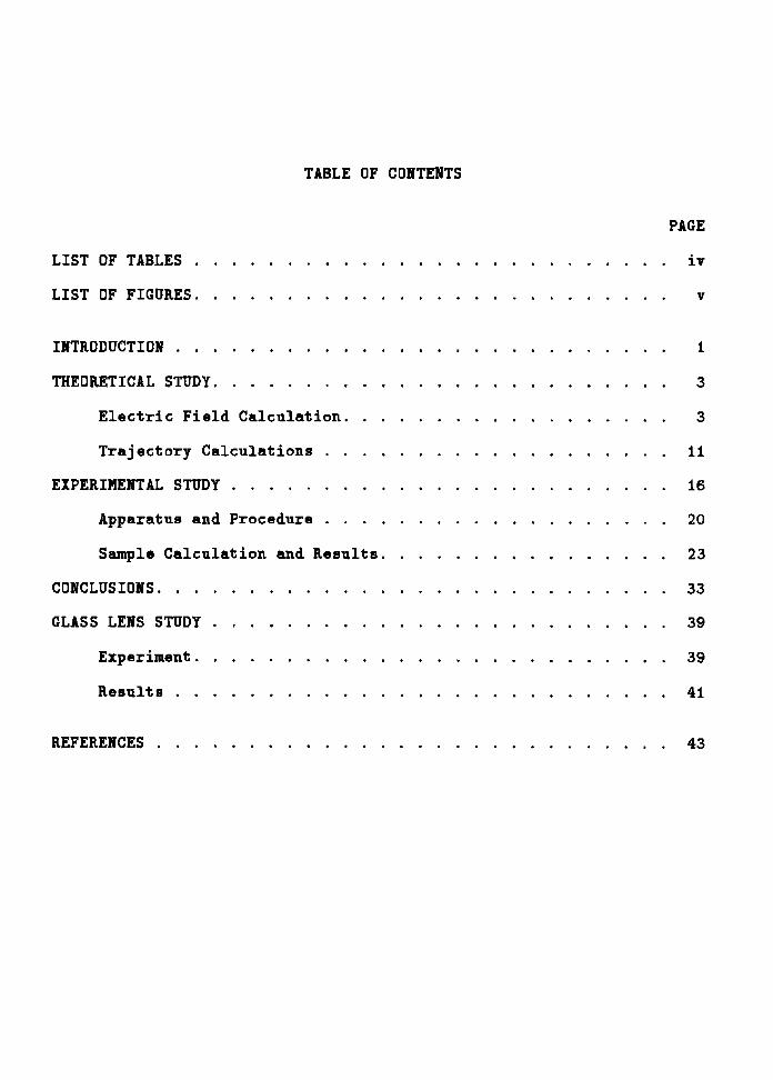
LIST OF TABLES .

LIST OF FIGURES ..

INTRODUCTION ..

THEORETICAL STUDY.

TABLE OF CONTENTS

Electric Field Calculation.

Trajectory Calculations .

EXPERIMENTAL STUDY . . . . . .

Apparatus and Procedure

Sample Calculation and Results ..

CONCLUSIOIS ...

GLASS LEIS STUDY .

Experiment ..

Results

REFERENCES .

PAGE

iv

v

1

3

3

11

16

20

23

33

39

39

41

43

LIST OF FIGURES

FIGURE

1. Three-ring Lena .

2. Lens Parameters

3. Potential due to a Hoop of Charge

4. Path through a Slice. . . . . . .

5. Optical System Ray Trace Parameters

6. Ray Trace for a Distant Source ...

7. Electron Optical Bench with Components.

8. Three-ring Lens Disassembled ..

9. Scale Drawing of Lens Assembly ..

10. Grating Shadow Pattern.

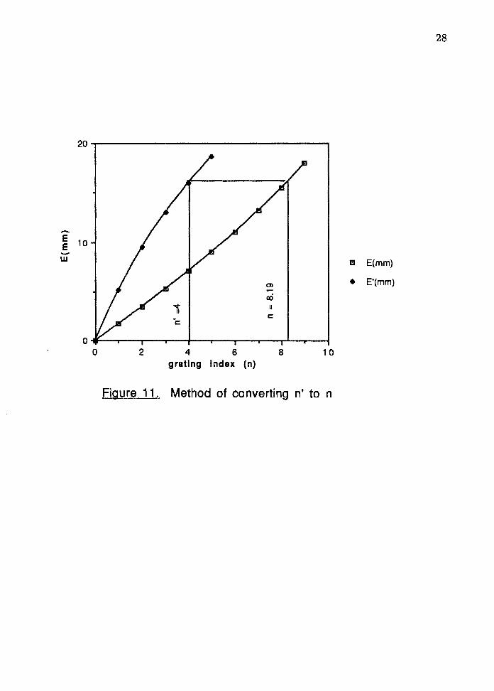
11. Method of Converting n' to n ..

12. Magnification Plot for Front Grating.

13. Magnification Plot for Rear Grating ..

14. Theoretical and Experimental Focal Length .

15. Theoretical and Experimental Focal Distance

16. Theoretical and Experimental Focal Length Aberration.

17. Theoretical and Experimental Focal Distance Aberration.

18. Experimental Apparatus for Glass Lens Study ..

19. Experimental Components for Glass Lens Study.

PAGE

4

5

7

13

17

19

21

22

24

25

28

29

30

34

35

36

37

40

40

LIST OF TABLES

TABLE PAGE

I Theoretical focal parameters . 15

II Experimental data. . . . . 26

III Experimental focal parameters. 32

IV Glass Lens Results . . . . . • 42

INTRODUCTION

Much of the science of electron optics depends on the fact that particles mov­

ing in a field of force can be focused in the same way that rays of light are focused by

a glass lens. This idea was first examined in 1828 when Hamilton [1 J brought atten­

tion to similarities between the equations that describe light rays passing through a

medium whose index of refraction varies in space and those that describe a particle

moving in a force field. The analogy was demonstrated experimentally in 1926 by

H. Busch [2] who used an axially symmetric magnetic field generated by a short coil

to focus electrons, and this was followed in the early 1930's by similar experiments

that used electric fields to accomplish the same results. The dual nature of waves

and particles was addressed theoretically in a paper by De Broglie [3] in 1924, and

in 1925 Davisson and Germer [4] observed diffraction effects from an electron beam

incident on a nickel crystal, verifying De Broglie's hypothesis. These breakthroughs

provided the experimental and theoretical groundwork for the development of the

many electron optical devices in use today. Some of these devices, such as the

electron microscopes, require high imaging reliability which in turn depends on the

focal properties of the electron lenses used in them. Therefore, there is contin­

ued interest in the study of electron lenses and the aberrations exhibited by them

which requires a detailed understanding of their electric and magnetic fields. For

electrostatic lenses, such as the one considered in this paper, this involves solving

Laplace's equation for a given set of electrode surfaces and potentials. The method

used in this paper to accomplish this is the charge density method described by

Renau, Read and Brunt [5]. It. has been used for the study of electron optical sys­

tems since 1963 [6] and has been further developed for this purpose up through the

2

early 1980's [7]. The method has several advantages over the older relaxation tech­

niques [8] which provide potentials only at discrete points in space, have a slower

convergence and require a large number of mesh points to give accurate solutions.

When the charge density method is applied to systems with cylindrical symmetry

the electrode surfaces are usually broken up into many thin flat rings of uniform

charge. A set of coupled linear equations is then generated by requiring appropri­

ate potentials on each ring in the presence of the other rings and the equations are

solved to find the charge on each ring. Finally, the rings are used with their charge

values to find the electric field. Normally this procedure requires the use of a digital

computer to solve the set of equations that determines the charge values but the

three-ring lens possesses a particularly simple electrode geometry which allows an

approximate closed-form expression to be found for the field near the axis. This

expression is derived and used in trajectory calculations which are used to find the

focal properties of the lens. The lens is then built and tested experimentally to

verify the predicted values. This study, therefore, provides a simple and illustrative

example of an electric field calculation using the charge density method.

THEORETICAL STUDY

In this study the theoretical focal properties of the three-ri11g electron lens are

determined. This is done by finding the electric field formed by the lens near its

axis (taking advantage of the planar and axial symmetry of the problem) and then

using Newton's second law of motion to calculate the trajectories of the electrons on

a digital computer. The parameters of the problem are shown in figures (1) and (2).

The field is found by using a variation of the charge density method, a method in

which the electrodes a.re replaced by thin strips of charge and the electric potential

is found from the values of the charges. The potential is expanded as a function

of the radial distance and a near-axis approximation for the field is found. Finally,

the trajectories are calculated by dividing the space of the lens into a large number

of cylindrical "slices", each having a constant field, and the equations of motion are

worked out in general for a slice, in a form suitable for use on a computer. The

focal properties are calculated for several ratios of cathode voltage to lens voltage,

Ve/Vi. The assumptions used are: 1) the electrons are confined to a region near

the axis of the lens and 2) polarization of charge on the electrodes of the lens has a

small effect on the trajectories.

ELECTRIC FIELD CALCULATION

The approach for finding the field is to replace each ring-shaped conductor

with an infinitely thin hoop of uniform charge, located at the center of the ring.

The values of the charges are then found by requiring the appropriate potentials

at selected locations which correspond to the portions of the surfaces of the rings

which are closest to the ax.is of symmetry. The first step is to find the potential in

x

·Ma!A uo!ioas sso.10 :s.1aiawe.1ed sua1 Bup-aa.141 'Z aJnl5!0d

0

u! osz· = 1 u! ooz· = M

U! 09G' = d

U! 00 ~· = l u, os~· = s u! oov· =a

z ~~1----------------------------------..-------1---- , . d

a

M

1 ,. _J?~

6

space due to a hoop of charge q whose radius is p (which is the mean radius of a ring

as shown in figure (2)) and whose center is located at the origin. The problem has

cylindrical symmetry so cylindrical coordinates a.re used. The potential is described

by

I dq V(p, ¢, z) = Ir - r,I (1)

where r 1 is the vector that points to the element of charge dq and r is the vector

that points to the location where the potential is being determined. In this case

dq = A d¢1 where ¢1 is the angle of integration and A = q /27r. These variables are

depicted in figure (3) with a perspective view. For the cylindrical symmetry shown

r 1 = p cos ¢1i + p sin <f>'J (2)

the hoop is at z = 0 but the point P is a distance z from the x-y plane so that

r = pcos<f>i + psin¢J+ zk (3)

and

(4)

This yields

I q 12'11" d<f>I V(p,¢,z) = --

41r€o 27r o VP2 + p2 + z2 - 2ppcos( ¢ - ¢1) (5)

setting </> = 0, substituting (} = ¢1 /2 and using the trig identity cos 29 = 2 cos2 (} - I

gives I 2q f'"/2 d(}

41r€o 7r lo V(P + p)2 + z2 - 4ppcos2 (} (6)

and now substituting t/J = 7r /2 - () and using the identity cos( 7r /2 - 0) = sin() gives

i 2q r12 dtt·

47r€o-; lo V(P + p)2 + z2 - 4ppsin2 t/J (7)

z

I I

I

I I

I

I

' I I

I

I I

I ,

(z'~'d)A~'i.s:;;;.....~~~~~~~~~~~"""""°"~--11--~-t ----,J • J

....... -...... -....... -......

which becomes

where

1 q k (i --;:::=d=l/J== 41rfo1r vPP lo /1 - k2 sin2 ¢

k = [ (1

4p/p Ji p/p)2 + (z/p)2

8

(8)

(9)

and the integral is a complete elliptic integral of the first kind, written from here

on as K(k) so that

V(p, z) = 4 2 q vPPkK(k)

1r t:o PP (10)

Now the values of the charges needed to simulate the rings can be found. A point

on each conductor surface, which is closest to the axis, is chosen and the potential

at each of these points is required to be equal to the voltage, Vi, on the conductor

that corresponds to it. The general equations for a system of conductors are

(11)

(12)

where Vii is the potential on the ith conductor due to the /h conductor and Aij is

a geometrical constant. For the three hoops this becomes

{13)

(14)

(15)

Since the system is symmetric about the midplane and the conductors are identical

(16)

(17)

(18)

9

(19)

a.nd equations {13), (14) and (15) can be rewritten a.s

(20)

(21)

(22)

where equations (20) and (22) are equivalent. Solving the first two gives

(23)

(24)

where

A 1 1 (21f dif/ (25) ij = 47r€o 27r Jo .j p2 + w2 + { Zi - z; )2 - 2pw cos(¢> - </>')

where w is the inner radius of the electrodes (which is where the potentials due to

the charges a.re required to agree with the voltages on the lens), pis the radius of

the hoops of charge a.nd the subscripts refer to the positions of the two conductors

along the z axis. Using the result previously worked out for a. hoop of charge this

becomes

where

4(w/p) (1 + (w/p))2 + ((zi - z;)/p)2

which for w/p = .80 a.nd (z2 - zi)/p = l/p 1.0 gives

1 An =

4 vPID(l.1348)

7r€o pw

(26)

(27)

(28)

10

A12 4

1J.Piii( .59871)

1rfo pw (29)

1 A13 = J.PW( .38258)

41rfo pw (30)

and finally since w = .200 inches and p = .250 inches

13 coulombs q1 = q3 = 47rfop(.5329)V0 = -3.763 x 10-

1 (Vo) (31)

VO t

13 coulombs q2 = -41rt:0p(l.351 )Vo= 9.541 x 10-

1 (Vo) (32)

VO t

and now the potential in space due to all three hoops is given by

(33)

where

(34)

and 4p/p

(35) (1 + p/p)2 ((z - zi)/p) 2

This can be used with the identity E = -VV to give the electric field at all points

in space (outside the conductors) in terms of complete elliptic integrals of the first

and second kind, but it is only necessary to know the field near the axis which is

found by using the series expansion

V(p,z) = V(O,z) - P2 a2V(O,z) + P4 a4V(O,z) - ... 4 8z 2 64 8z4

together with the on-axis potential due to one hoop of charge at the origin

q V(O,z)=

41rt:ovf P2 + z2

keeping the first three terms of the equation (35) gives the approximation

q [ p2 1 3z2

V(p,z) ~ 41rt:oJP2 + z2 1+4((p2 + z2) (p2 + z2)2)

p4

( 9 90z2 105z4 ]

+ 64 (p2 z2)2 - (p2 + z2)3 + (p2 + z2)4)

(36)

(37)

(38)

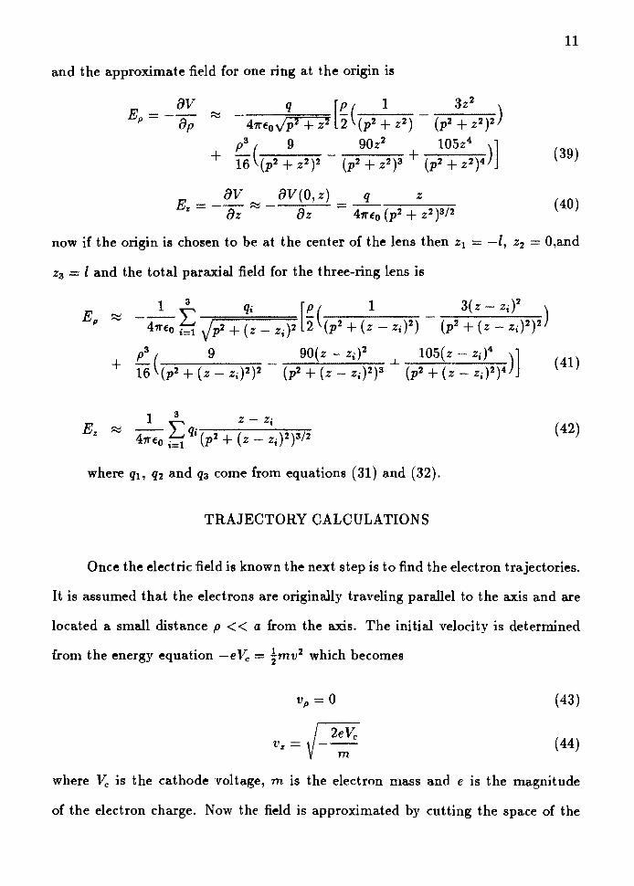
and the approximate field for one ring at the origin is

E __ av p - op

av Ez = -- ~ oz

8V(O,z) q

OZ = 411'Eo (p2

11

(39)

z (40)

now if the origin is chosen to be at the center of the lens then z1 = -l, z2 O,and

z3 = l and the total paraxial field for the three-ring lens is

(41)

(42)

where qi, q2 and q3 come from equations (31) and (32).

TRAJECTORY CALCULATIONS

Once the electric field is known the next step is to find the electron trajectories.

It is assumed that the electrons are originally traveling parallel to the axis and are

located a small distance p < < a from the axis. The initial velocity is determined

from the energy equation -e Ve = !mv2 which becomes

(43)

(44)

where Ve is the cathode voltage, m is the electron mass and e is the magnitude

of the electron charge. Now the field is approximated by cutting the space of the

12

lens into thin cylindrical "slices" and then treating each slice as having a constant

field,Ep and E.,, which is evaluated at the point where the electron would cross the

center of the slice if no forces acted on it (see figure 4). From Newton's second

law of motion, F = ma, and the assumption that there is no ¢ component in the

velocity

(45)

(46)

and this immediately leads to the set of equations that describe the motion in a

given slice (the ith slice) of the field.

(47)

(48)

(49)

(50)

where

(51)

(52)

since the width of the slice ,i+1 zi, is known, ti can he found from equation ( 47)

i (.!i-)2 2

(zitl_zi) if Ai > O· -~+ A• A• + A• z ' • • • ti= (53)

v• (.!i-)2 2(zi+l_zi) otherwise. _..:;+ -A• A• + A• • • •

where the postive root for A: < 0 is not included because it corresponds to the case

where the electron is reflected, which does not occur in this problem. Now ti can

r i

I I I

__ VE(r,zi

,.,.-"' I vi+1 ,,. I J Vy- ~----------

~----\-~- . . --- , ,-----.. 1 · I ~ro1ect1on

actual path

r i+1

z i zi+1

Figure 4. Path through a slice of the lens field.

13

14

be used in equations ( 47),( 49) and (50) to update p,vP and Vz for each slice iteratively

throughout the field of the lens to give the trajectory as a function of time.

For the results presented in table (I) the lens field is divided into 10,000 sections

and the equations of motion are solved for each section. Once the electron is outside

the field of the lens, its final direction is projected back onto the axis to find the

focal point. This is repeated for ten rays entering at different radial distances. Thus

the focal length and focal distance are found as a function of the radial height of

the ray at the principle surface, p. The paraxial values,10 and g0 , and their second

order aberrations, S1 and 89 , are then found from these functions as defined by the

equations

Al_ S1p2

lo - IJ Ag_ S9p2

lo - fJ

(54)

(55)

15

TABLE I

THEORETICAL FOCAL PARAMETERS

I V,/Vc II fo(in) I go(in) I s, 1.00 1.25 1. 22 0.95 1.46 1.44 0.90 1. 72 1. 70 0.85 2.04 2.02 -185 -186 0.80 2.42 2.40 -253 -254 0.75 2.90 2.88 -350 -351

EXPERIMENTAL STUDY

In this study the two-grating method of Spangenburg and Field [9] is used

to determine the focal properties of the electron lens. This method, which is ex­

tended by Rempfer [10] to include calculation of the spherical aberrations, consists

of placing two fine wire gratings in the beam path outside the lens and analyzing

the magnified shadow pattern cast by them on photographic film. One grating is

placed in the field free space in front of the lens and the other in the field free space

behind the lens. The gratings are rotated relative to each other by ninety degrees

so that the patterns formed by them are distinguishable from each other. Thus the

rays in the object and image space of the lens can be traced and the focal properties

determined. The experimental arrangement and parameters are shown in figure (5)

which shows a ray coming from a small source a distance z away from the center

of the lens, passing through the lens, forming a demagnified image at z' and finally

falling on a viewing screen some distance away. The front grating is a distance a

from the source, and the back grating is a distance b from the center of the lens

and d from the viewing screen. The lens is a unipotential lens with symmetery

about its midplane, therefore the center is also the location of the reference plane

which is chosen to be midway between its focal planes. The height of a given ray

from the axis as it passes through a grating is e for the front grating and e' for

the back grating, and E is its height as it reaches the viewing screen. The image

magnification therefore is

where

Cl:'. m=­

a' (56)

ll

en '< en ..... CD 3

..... .... fl) 0 CD

"'O fl) .... fl)

3 CD ..... CD ...... en

N ..

n

a.

-------

-----­ ...-...

aomos u0Jioe13

aoJnos JO e6ew1

eue1d Mope4s

18

c = b - z' d

1 (57)

where M = E / e and M' = E / e'. In this study it is assumed that the spacings in

each grating are equal, i.e. e = ne1 where e1 is the spacing between two consecutive

wires in a grating. The case where the source is distant and the incoming rays

are parallel to the axis is shown in figure (6), which defines the nomenclature for

the focal properties of the lens. For the general case the focal length f and focal

distance g can be found from z - z'

f = 1/m-m (58)

g = z' - fm (59)

These quantities as a rule will vary with the height of the incoming rays due to

spherical aberration, which manifests itself as distortions in the grating shadow

patterns. Therefore rays entering the lens parallel to the axis at different heights

will cross the axis at different positions and the principle surfaces Hand H' will be

curved rather than planar. The spherical aberration in this experiment is predom­

inantly second order, therefore the shadow magnifications can be expressed with

sufficient accuracy by

(60)

(61)

where n can be found for equation (61) by plotting E vs. n and n', and converting

n' into n for a given E value.

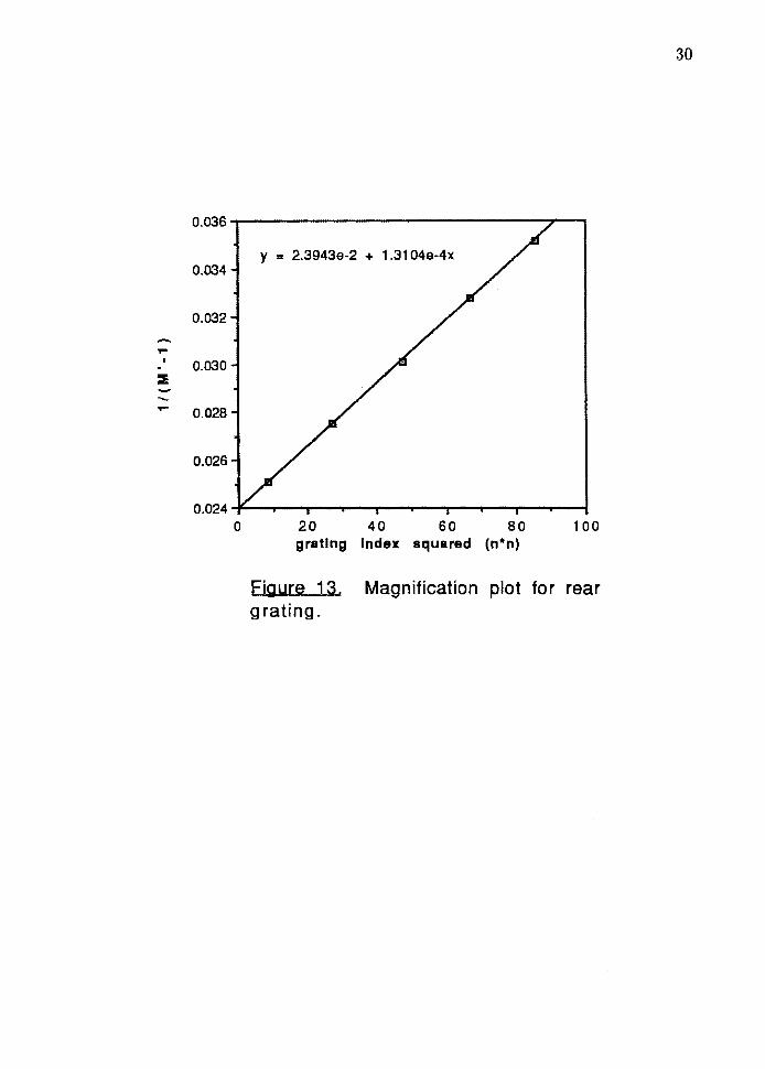
The distortion coefficients, /3 and /3', and the paraxial magnifications, M 0 and

M~, are found by plotting M vs n 2 and ( M' - 1)-1 vs n 2• Substituting the values

M 0 and M~ into the previous equations gives the paraxial values z&, m 0 , fo and

aomos lLIElS!P e JOJ aoEJl AB!:::I ·g 0Jhf5!,:j

6 -0US1d --90U0J0l0t:I

\ \ I

\ I

-\ I

H -\ I ...,;

.H \ I

\ I

I I

I I

I I

._J_ I I

~ I I

I I

·~ I I

I I

.:I I I :I

"" ... I I

"" I I

d ~ ....... \

I ...... I

I .......... I

, I "" \

I I ... ... \

I ------1-----":. - -- I I j . \

~ -

-. - -

I -

-.

61

20

g0 , and the variations of focal length and focal distance can be described to second

order by

1 )2 2 - a mo

1 )2 2 - a mo

(62)

(63)

Where pis the radial offset of the incoming ray from the axis at the principle surface,

and S 1 and Sg are the dimensionless spherical aberration constants. Expressing

these coefficients in terms of the experimental quantities gives

_ ( C2 - 2moC1) /( / 1 ) 2 (l _ m~) P1 JO

(64)

(65)

where C1 = f3 - (31 / M~, C2 = cof3' /lo and P /lo (1 1/m0 )0:1 where 0:1 = eif a.

APPARATUS AND PROCEDURE

An electron optical bench is used to hold the lens and other components in

alignment with respect to each other. The bench is essentially a long horizontal

vacuum chamber with veeways to support electron optical components, mechanical

linkages to allow the components to be moved from outside the bench and electrical

feedthroughs to provide the voltages needed by the source and lenses. An oblique

end-view of the bench is shown in figure (7) with the components in place. At the

far end in the veeways is a triode electron gun which served as the source for the

experiment. Partly visible in the front is an aluminized phosphor-coated fiber optics

window which allows the shadow images to be seen and recorded from ouside the

bench. The disassembled three-ring lens is shown in figure (8). The three machined

brass electrodes are arranged in order below the rexolite spacers that hold them in

place and the lens housing is to the left. A scale drawing of the lens assembly is

21

Figure 7. Electron optical bench with components

22

'·

Figure 8. Three-ring lens disassembled

23

given in figure (9) for completeness. The electron beam begins at the triode gun

and then passes through a condenser lens which focuses it onto an aperture. This

aperture serves as the effective source for the experiment. The beam then passes

through the front grating, three-ring lens and rear grating before it finally reaches

the fiber-optics window where a visible image is formed.

The experimental focal properties of the three-ring lens were determined for six

different lens voltages. The accelerating potential was 20 kV for all cases. The ratios

of lens potential to accelerating potential, Vi/Ye, used were 1.0,.95,.90,.85,.80 and

. 75. The bench pressure was less than 10-4 torr. For the first lens voltage, Vi/Ye =

LO, the front grating position was adjusted so that about 20 grating shadows were

observed and was not changed for the rest of the experiment. For each voltage the

position of the rear grating was adjusted so that: 1) it was close enough to the

image formed by the lens so that distortion was measurable and 2) enough shadow

images were visible to reduce the error due to individual variations in the grating

spacings. To accomplish this it was necessary in some cases (Vi /Ve = .85, .80, . 75) to

place the grating on the lens side of the source image. This caused the distortion in

the rear grating shadow to change from barrel to pincushion. Photographic film was

placed in contact with the outside of the fiber optics window to record the pattern

for each run. The recorded patterns were then measured and the data analyzed to

find the focal properties for each case.

SAMPLE CALCULATION AND RESULTS

The data and calculations are included here for the case where Vi/Ye .95

to demonstrate how the experimental values / 0 , g0 , S1 and S9 were obtained. The

shadow pattern for this case is shown in figure (10) and the data taken from the

pattern is listed in table (II). The positions of the shadows cast by the front grating

END ELECrnODE

_, .150" r- -I i.- .100·

I'-- .1 oo·

CENTER ELECTRODE

I I I

~

--- .400"

_l .050·

8'10 8.ECTRODE

-..j I-- .050" .350"----1

figure 9. Scale drawing of lens assembly.

24

-=It~ ~-~~ v).,, Ive.::: e. q s--

,.111iii i.i,, ............ ,,~ ~ ......... ~ .. .. . ~~~ ............... '

1111lllllllllllHll • 11111111111111::::: ! , .................. . , ............... , ................. ......... __

~-····

Figure 10. Grating shadow pattern. Distortions in the pattern (otherwise a grid of rectangles) are manifestations of the lens aberrrations. The two protrusions on top are from clips which held the gratings in place.

25

TABL

E II

EXPE

RIM

ENTA

L DA

TA

0 27

.14

8 2

7.1

48

0

0 2

5. 1

14

25

.11

4

0 0

0 1

28

.85

9

25

.40

0

1.7

30

1

3.6

2

1 3

0.2

38

1

9.8

59

5

.19

0

2.9

3

2.5

1

8.5

8

---·

2 3

0.6

53

2

3.6

71

3

.49

1

13

.74

2

34

.47

3

15

.49

8

9.4

88

5

.22

2

.75

2

7.2

·······-~---

·-···

·----

----·-

---.-

---·-

3 32

.45

2

21

. 87

8

5.2

87

1

3.8

8

3 3

7.9

49

1

1. 8

62

13

.04

6

.88

3

.01

4

7.3

·-

----

----

----

----

---

4 3

4.3

28

2

0.0

84

7

.12

2

14

.02

4

41

.01

3

9.0

09

1

6.0

0

8.1

9

3.2

8

67

.1

--

---------

---·

··-·

-·--

36

.31

2

18

.22

6

9.0

43

1

4.2

4

5 4

3.7

70

6

.35

6

18

.71

9

.25

3

.51

------·---

6 3

8.3

83

1

6.2

83

1

1. 0

50

14

.50

~--

----

~---··---·--

7 4

0.6

25

1

4.2

10

1

3.2

07

1

4.8

6

8 4

3.0

37

1

2.0

03

1

5.5

17

1

5.2

7

------~·

----------~----------~-

9 4

5.6

15

9

.59

0

18

.01

3

15

.76

27

are known as a function of the front grating index n and the positions on either side

of the center are averaged to give E. Likewise the positions of the shadows cast by

the rear grating E' are known as a function of the rear grating index n' and are

averaged to give E'. The relationship between n and n' is found by plotting E vs

n and E vs n' as shown in figure ( 11). Now the shadow magnifications are found

from M = E/ne and M = E/n'e, where the spacing on the electron bar grids used

is e = 125µm, and plots are made of M vs n 2 and ( M' - 1 t 1 vs n 2• These plots are

shown in figures (12) and (13) and are linear as expected. The slope and intercept

values from the plots are used with equations (60) and (61) to give the paraxial

magnifications and distortion coefficients which are

M 0 = 13.6

M~ = 43.0

f3 = 1.92 x 10-3

/3' = 5.63 x 10-3

The measured distances corresponding to figure ( 5) for this case are

a= 11.370 in

z = 12.355 in

b = 1.846 in

d = 17.196 in

and finally these values are used in equations ( 55) through ( 64)

Jo= 1.259

to obtain

8('.;

(ww).3 •

(ww)3 m

o~ 9 (u) xepu1 6unaJ6

9 p

m - o~ 3 3

29

y = 13.607 + 2.6079e-2x

15

14

13 0 20 40 60 80 100

grating Index squared (n*n)

Eigure 12. Magnification plot for front grating

,.. I

-. ,..

y = 2.3943e-2 + 1.3104e-4x 0.034

0.032

0.030

0.028

0.026

0.024 ~-----.--------.,----,--..----. 0 20 40 60 80 100

grating Index squared (n*n)

Figure 13. Magnification plot for rear grating.

30

g0 = 1.293

s, = -87.6

89 = -77.9

31

Most of the error in this method is due to variations in the grating spacings.

These errors are carried through into the graphs used for finding the shadow mag­

nifications and the distortion coefficients. It is for this reason that the effort was

made to include as many grating shadows as possible. If the variations are randomly

distributed then the intercept errors should scale down with 1/./N where N is the

total number of grating shadows measured. Another way to reduce this error is to

measure the individual grating spacings and use the individual e values. Table (III)

gives the experimental focal properties for six voltage ratios from Vi/Ye = .75 to

Vi/Vc = 1.00.

32

TABLE III

EXPERIMENTAL FOCAL PARAMETERS

Vi/Yc II /o(in) g0 (in) St s, 1.00 1.06 1.07 -64.8 -50.3 0.95 1.26 1.29 -81.6 -77.9 0.90 1.50 1.50 -121 -65.3 0.85 1. 78 2.85 -158 -167 0.80 1.99 I 2.08 -177 -228 0.75 2.39 2.56 -179 -433

CONCLUSIONS

Graphs of the predicted and experimentally measured values for focal length,

focal distance, and the spherical aberrations of these quantities are shown in fig-

ures (14),(15),(16) and (17) in pairs for direct comparison. The two sets of data

show reasonable agreement. Some offset is expected because the theoretical study

neglected two effects which are known to be present in the experiment : 1) polar-$

ization of charge on the electrodes and 2) the presence of the disc-like exten~ns

on the electrodes. The main effect of charge polarization is to shift the centroids of

the charges on the rings so that they are closer together. In the theoretical study

this is equivalent to placing the hoops closer together which tends to increase the

focal length and focal distance, and therefore is clearly not the dominating effect.

The disc-shaped extensions on the electrodes, on the other hand, give the lens a

larger total capacitance which increases the charge present on each electrode. This

could also increase the charge residing on each ring, thereby increasing the strength

of the lens. However, without a more detailed calculation it is difficult to say just

how the increased charge distributes itself, i.e. whether it is mostly on the ring or

the disc portion. The experimental results suggest that it is on the ring.

The manner in which the focal properties change with voltage is consistent

between the two sets of curves. Figure (17) shows that the focal distance aberration

is undercorrected, which is true for all electrostatic lenses. From the theoretical

data it is evident that the focal length f is always greater than the focal distance

g and ,therefore, the principle surfaces H and H' are crossed for all the voltages

used. The experimental values, however, are not as dear on this point because the

experimental error is greater than the actual difference between f and g. The

-., Ill .r. g 2

0 - m TH:fO

• EXP:fO

1.00 .95 .90 .85 .80 .75 VI/Ve

Figure 14. Theoretical and experimental focal length

34

o6:dx3 • o6:HJ.. m

aoueJS!P 1eoo1 1e1uawpadxa pue 1eo!JaJoa41 ·g ~ EUn0!3

OAflA

SL' 08' sa· 05· 96" oo· ~

-ti)

o-.------~~----------

-100

-200

-300

-400 -l---..---r---.--r---r-r--r---r-..,.---r--.. 1.00 .95 .90 .85 .80 .75

VI/Ve

Figure 16. Theoretical and experimental focal length aberration

m TH:Sf

• EXP:Sf

36

-100

m (() .. ::c -200 t-

-300

l!I

•

1.00 .95 .90 .85 .80 .75 VI/Ve

Figure 17. Theoretical and experimental focal distance aberration

37

TH:Sg

EXP:Sg

38

simplified charge density method used for the theoretical study shows good qualita­

tive agreement with the experiment and with the known properties of electrostatic

lenses.

GLASS LENS STUDY

In this section the two-grating method discussed previously is used to measure

the focal properties of a planoconvex glass lens, first with the flat side facing the

source and then with the curved side facing the source. Throughout this section

these two situations are referred to as configuration 1 and configuration 2, respec­

tively. The results from this experiment are compared with ray trace calculations

based on the index of refraction, thickness and radius of curvature of the lens to

provide the reader with a sense of the accuracy and reliability of the method.

EXPERIMENT

The two gratings used were photograph negatives with evenly spaced alter­

nating clear and dark bars. These bars were measured with a traveling microscope

and were found to have a spacing of e1 = e~ = .1953 cm. The grids were then

mounted on glass plates whose thicknesses were .30 cm each. The gratings were

then mounted in holders so that they were oriented 90 degrees apart from each

other. The plates, source, guide tube and lens were then mounted on an optical

bench with a grating on either side of the lens. The source used was a concentrated

arc lamp which produced a very bright (bluish) small circular spot at the end of its

3.58 cm bulb. The screen was in contact with the edge of the optical bench which

was 3.8 cm from the 125 cm mark on the bench. Photographs of the components

and the experimental arrangement are shown in figures (18) and (19). The distances

between elements were all measured to within 0.5 mm. The description up to this

point refers to configuration 1. For configuration 2 all the elements were in the

same posit.ions except that the lens was turned around so that its curved side faced

Figure 18. Experimental apparatus for glass lens study

Figure 19. Experimental components for glass lens study

41

the source while its fl.at side remained in the same position as before. Photographic

print paper was then placed on the screen with the apparatus in a dark room and

the source was turned on for about six minutes for each case. The prints containing

the grating patterns were then developed and the distances between the shadows

were obtained with a ruler and recorded.

RESULTS

The experimental and calculated focal properties of the lens for both con­

figurations are presented in table (IV). The values for the discrepancies are also

included because in this study, unlike the electron lens study, the theoretical and

experimental results are expected to agree. The focal lengths are smaller than the

focal distances in all cases, which is normal for a glass lens. The longitudinal spher­

ical aberration f::..z' / p2 for configuration 1 is about twice that for configuration 2

and both values agree very well with the ray trace calculations. This is due to the

fact that the object is further away from the lens than the image and, therefore,

the angles of deviation are minimized, in a least squares sense, when the curved

side of the lens faces the source. The focal lengths had a 1 % discrepancy, the focal

distances agreed to about 2 % and the spherical aberrations agreed to within 8 %.

Much of this error can be attributed to the fact that a white light source was used.

There is also error associated with the finite size of the source which manifests itself

as "smearing" of the shadow patterns. It is expected that if a laser were used in

place of the source the agreement would be even better.

42

TABLE IV

GLASS LEIS RESULTS

TWO-GRATING METHOD

I Configuration II /0 (cm) I go (cm) j 6.z' / p2 cm-1 I 1 15.75± .42 16.48 ± .47 -.3415 2 15.77 ± .56 16.44 ± .66 -.1763

RAY-TR.A.CE CALCULATIONS

Configuration fo (cm) go (cm) 6.z' / p2 cm-1

1 15.60 ± .69 16.10 ± .69 -.358 2 15.60 ± .69 16.10 ± .69 -.163

DISCREPANCIES

I Configuration II fo (Y.) 90 (Y.) 6.z' Ip" <Y.)

I ~ II 1.0 2.3 4.7 1.1 2.1 7.8

REFERENCES

1. Paszkowski, B.,1968, Electron Optics, Elsevier Publishing Company Inc., Nev York, p. 2

2. Busch, H., 1926, Annalen der Physik, Vol 81, p 974

3. De Broglie, P. M., 1924, 47, p 446

4. Davisson, C. J., and L. H. Germer, 1927, Phys. Rev., Dec. 30,705, Bell Laboratories Record, Vol. 4, No. 2, Apr. 1927, pp. 257-260

6. Renau, A., F. H. Read and J. N. H. Brunt, 1981, J. Phys. E:Sci. Instrum., 15, pp. 347-54

6. Cruise, D.R. , 1963 J. Appl. Phys., 34, pp. 3477-9

8. Singer, B., and M. Braun, 1970, IEEE Trans. Elec. Devices, ED-17, p 926

9. Spangenberg, K. , and L. M. Field, March 1942, Proceeding of the IRE, 30, pp. 138-144

10. Rempfer, G. F., 1985, J. Appl. Phys., 57, p 2385