a theoretical framework for deep transfer learningwolf/papers/transferablefinal.pdfa theoretical...
TRANSCRIPT

A Theoretical Framework for Deep Transfer Learning
Tomer GalantiThe School of Computer ScienceTel Aviv [email protected]
Lior WolfThe School of Computer ScienceTel Aviv [email protected]
Tamir HazanFaculty of Industrial Engineering & [email protected]
Abstract
We generalize the notion of PAC learning to include transfer learning. In ourframework, the linkage between the source and the target tasks is a result of hav-ing the sample distribution of all classes drawn from the same distribution of dis-tributions, and by restricting all source and a target concepts to belong to the samehypothesis subclass. We have two models: an adversary model and a randomizedmodel.In the adversary model, we show that for binary classification, conventional PAC-learning is equivalent to the new notion of PAC-transfer and to transfer generaliza-tion of the VC-dimension. For regression, we show that PAC-transferability mayexist even in the absence of PAC-learning. In the randomized model, we providePAC-Bayesian and VC-style generalization bounds to transfer learning, includingbounds specifically derived for Deep Learning. A wide discussion on the tradeoffsbetween the different involved parameters in the bounds is provided.We demonstrate both cases in which transfer does not reduce the sample size(“trivial transfer”) and cases in which the sample size is reduced (“non-trivialtransfer”).
1 Introduction
The advent of deep learning has helped promote the everyday use of transfer learning in a variety oflearning problems. Representations, which are nothing more than activations of the network units atthe deep layers, are used as general descriptors even though the network parameters were obtainedwhile training a classifier on a specific set of classes under a specific sample distribution. As aresult of the growing popularity of transferring deep learning representations, the need for a suitabletheoretical framework has increased.
In the transfer learning setting that we consider, there are source tasks along with a target task. Thesource tasks are used to aid in the learning of the target task. However, the loss of the source tasksis not part of the learner’s goal. As an illustrative example, consider the use of deep learning forthe task of face recognition. There are 7 billion classes, each corresponding to a person, and eachhas its own indicator function (classifier). Moreover, the distribution of the images of each classis different. Some individuals are photographed more casually, while others are photographed informal events. Some are photographed mainly under bright illumination, while the images of othersare taken indoors. Hence, a complete discussion of transfer learning has to take into account boththe classifiers and the distribution of the class samples.
A deep face-recognition neural-network is trained on a small subset of the classes. For example,the DeepFace network of Taigman et al. (2014) is trained using images of only 4030 persons. Theactivations of the network, at the layer just below the classification layer, are then used as a generictool to represent any face, regardless of the image distribution of that person’s album images.
1

In this paper, we study a transferability framework, which is constructed to closely match the theoryof the learnable and its extensions including PAC learning (Valiant, 1984) and VC dimension. Afundamental Theorem of transfer learning, which links these concepts in the context of transferlearning, is provided. We introduce the notion of a simplifier that has the ability to return a subclassthat is a good approximation of the original hypothesis class and is easier to learn. The conditions forthe existence of a simplifier are discussed, and we show cases of transferability despite infinite VCdimensions. PAC-Bayesian and VC bounds are derived, in particular for the case of Deep Learning.A few illustrative examples demonstrate the mechanisms of transferability.
A cornerstone of our framework is the concept of a factory. Its role is to tie together the distributionsof the source tasks and the target task without explicitly requiring the underlying distributions tobe correlated or otherwise closely linked. The factory simply assumes that the distribution of thetarget task and the distributions of the source tasks are drawn i.i.d from the same distribution ofdistributions. In the face recognition example above, the subset of individuals used to train thenetwork are a random subset of the population from which the target class (another individual) isalso taken. The factory provides a subset of the population and a dataset corresponding to eachperson. The goal of the learner is to be able to learn efficiently how to recognize a new person’s faceusing a relatively small dataset of the new person’s face images. This idea generalizes the classicnotion of learning in which the learner has access to a finite sample of examples and its goal is to beable to classify wisely a new unseen example.
2

Table 1: Summary of notationsε, δ error rate and confidence parameters ∈ (0, 1)X instances setY labels setZ examples set; usually X ×Yp a distributiond a task (a distribution over Z)k the number of source tasksm the number of samples for each source taskU a finite set of distributions; usually U = d1, ..., dk or U = p1, ..., pk
E′ a set of distributions over XE an environment, a set of tasksprobp(X) or p(X) the probability of a set X in the distribution pP,E the probability and expectation operatorsP[X|Y],E[X|Y] the conditional probability and expectationD[K] or justD a distribution over distributions (see Definitions 3, 4)K the subject of a factorys = z1, ..., zm data of m examples ∀i : zi ∈ ZS = (s[1,k], st) k source data sets s1, ..., sk (of same size) and one target data set sto = x1, ..., xm data of m instances ∀i : xi ∈ X
O = (o[1,k], ot) data of k of unlabeled source data sets o1, ..., ok (of same size)and one target data set ot
S ∼ D[k,m, n] data set S according to the factoryD with sizes∀i ∈ [k] : |si| = m and |st | = n
S ∼ D[k,m] source data set S according to the factoryD with sizes∀i ∈ [k] : |si| = m
U ∼ D[k] set of tasks of size k taken fromDd ∼ D a task taked fromDH a hypothesis class (in the supervised case, a set of functions X → Y)c a concept; an item ofHC a hypothesis class family; a set of subsets inH such that
H =⋃
B∈C BB a bias; i.e, B ∈ C (and B ⊂ H)N an algorithm that outputs hypothesis classesA an algorithm that outputs conceptsr(s) the application of an algorithm r on data s` : H × Z → R a loss function0-1 loss `(c, (x, y)) = ([c(x) = y] = true)squared loss `(c, (x, y)) = (c(x) − y)2/2T a learning setting; usually T = (H ,Z, `)TPB a PAC-Bayes setting; usually TT B = (T,Q, p)T a transfer learning setting; usually T = (T,C ,E)εd(c) the generalization risk function = the expectation of `(c, z),
i.e, Ez∼d[`(c, z)]εs(c) the empirical risk function; εs(c) = 1
|s|∑
z∈s `(c, z)g : C × E → R the infimum risk g(B, d) = infc∈B εd(c) = infεd(c) : c ∈ BεD(B) transfer generalization risk = Ed∼D[g(B, d)]εU(B) source generalization risk = 1
|U |∑
d∈U[g(B, d)]εs(B, r) 2-step empirical risk = εs(rB(s))εS (B, r) 2-step source empirical risk = 1
k∑k
i=1[εsi (rB(si))]R(q) randomized transfer risk = EB∼q[εD(B)]RU(q) randomized source generalization risk = EB∼q[εU(B)]KL(q||p) KL-divergence, i.e, KL(q||p) = Ex∼q[log(q(x)/p(x))]εp(c1, c2) the mutual error rate; εp(c1, c2) = ε(p,c1)(c2)εo(c1, c2) the mutual empirical error rate; εo(c1, c2) = εc1(o)(c2)errp(B,K) the compatibility error rate; errp(B,K) = supc1∈K infc2∈B εp(c1, c2)erro(B,K) the empirical compatibility error rate; erro(B,K) = supc1∈K infc2∈B εo(c1, c2)
3

Table 2: Summary of notations (continued)EU(B,K) the source compatibility error rate; EU(B,K) = 1
|U |∑
p∈U errp(B,K)E(B,K) the generalization compatibility error rate; E(B,K) = Ep∼D[errp(B,K)]EO(B,K) the source empirical compatibility error rate; EO(B,K) = 1
|O|∑
o∈O erro(B,K)hV,E,σ,w a neural network with architecture (V, E, σ) and weights w : E → RHV,E,σ set of all neural networks with architecture (V, E, σ)H I
V,E,σ family of all subsets ofHV,E,σ determined by fixing weights on I ⊂ EE = I ∪ J a set of edges in a neural network, I is the set of edges in the transfer
architecture and J the rest of the edges (i.e, I ∩ J = ∅)HV,E, j,σ the architecture induced by (V, E, σ) when taking only the first j
layers (see Section 6)ERMB(s) empirical risk minimizer; ERMB(s) = arg minc∈B εs(c)C-ERMC (s[1,k]) class empirical risk minimizer;
C-ERMC (s[1,k]) = arg minB∈C1k∑k
i=1 minc∈B εsi (c)c∗i,B empirical risk minimizer in B for the i’th data set; c∗i,B = ERMB(si)ri,B the application of a learner rB of B on si; ri,B = rB(si)u||v concatenation of the vectors u, v0s a zeros vector of length s1 a unit matrixNu(ε, δ) a universal bound on the sample complexity for learning any hypothesis class
of VC dimension ≤ uEh the set of all disks around 0 that lie on the hyperplane hvc(H) the VC dimension of the hypothesis classHτH (m) the growth function of the hypothesis classH ;
i.e, τH (m) = maxx1,...,xm∈Xm
∣∣∣∣(c(x1), ..., c(xm)) : c ∈ H∣∣∣∣
τ(k,m, r) the transfer growth function of the hypothesis classH ;i.e, τ(k,m, r) = maxs1,...,sk∈Z
mk
∣∣∣∣(r1,B(s1), ..., rk,B(sk)) : B ∈ C ∣∣∣∣
τ(k,m; C ,K) the adversary transfer growth function;i.e, τ(k,m; C ,K) = maxo1,...,ok∈X
mk∣∣∣∣c1,1(o1), c1,2, ..., ck,1(ok), ck,2(ok)) : ci,1 ∈ K and ci,2 = ERMB(ci,1(o)) s.t B ∈ C∣∣∣∣
4

2 Background
In this part, a brief introduction of the background required is provided. The general learning frame-work, the PAC-Bayesian setting and deep learning are introduced. These subjects are used andextended in this work. A reader who is familiar with these concepts, may skip to the next sections.
The general learning setting Recall the general learning setting proposed by Vapnik (1995). Thissetting generalizes classification, regression, multiclass classification, and several other learningsettings.Definition 1. A learning setting T = (H ,Z, `) is specified by,
• A hypothesis classH .
• An examples set Z (with a sigma-algebra).
• And a loss function ` : H × Z → R.
This approach helps to define supervised learning settings such as binary classification and regres-sion in a formal and very clean way. Furthermore, in this framework, one can define learning sce-narios when the concepts are not functions of examples, but still have relations with examples fromZ measured by loss functions (e.g, clustering, density estimation, etc.). If nothing else is mentioned,T stands for a learning setting. We say that T is learnable if the corresponding H Is learnable. Inaddition, ifH has a VC dimension d, we say that T also has a VC dimension d. With these notions,we present an extended transfer learning setting, as a special case of the general learning setting witha few changes.
If a distribution d over Z is specified, the fitting of each c ∈ H is measured by a Generalization Risk,εd(c) = Ez∼d[`(c, z)]
Here, H , Z and ` are known to the learner. The distribution d is called a task and is kept un-known. The goal of the learner is to pick c ∈ H that is closest to infc∈H εd(c). Since the distributionis unknown, this cannot be computed directly and only approximated using an empirical data setz1, ..., zm selected i.i.d according to d. In many machine learning algorithms, the empirical riskfunction, εs(c) = 1
m∑
z∈s `(c, z) has great impact in the selection of the output hypothesis.
Binary classification: Z = X × 0, 1 andH consisting of c : X → 0, 1 with ` a 0-1 loss.Regression: Z = X × Y where X and Y are bounded subsets of Rn and R respectively. H is a set
of bounded functions c : X → R and ` is any bounded function.
One of the early breakthroughs in statistical learning theory was the seminal work of Vapnik & Cher-vonenkis (1971) and the later work of Blumer et al. (1989), which characterized binary classificationsettings as learnable if and only if the VC dimension is finite. The VC dimension is the largest sizerequired to ensure that there is a set of examples (of that size) such that any configuration of labelson it is consistent with one of the functions inH .
Their analysis was based on the growth function,
τH (m) = maxo∈Xm
∣∣∣∣c(x1), ..., c(xm) : c ∈ H∣∣∣∣, where o = x1, ..., xm
A famous Lemma due to Sauer (1972) asserts that whenever the VC dimension of the hypothesisclassH is finite, then the growth function is polynomial in m,
τH (m) ≤(
emvc(H)
)vc(H)
when m > vc(H) (1)
Theorem 1 (Vapnik & Chervonenkis (1971)). Let d be any distribution over an examples set Z,Ha hypothesis class and ` : H × Z → 0, 1 be the 0-1 loss function. Then
Es∼dm
[supc∈H
∣∣∣∣εd(c) − εs(c)∣∣∣∣] ≤ 4 +
√log(τH (2m))√
2m
In particular, whenever the growth function is polynomial then the generalization risk and empiricalrisk uniformly converge to each other.
5

PAC-Bayes setting The PAC-Bayesian bound due to McAllester (1998) describes the ExpectedGeneralization Risk (or simply expected risk), i.e, the expectation of the generalization risk withrespect to a distribution over the hypothesis class. The aim is not measuring the fitting of eachhypothesis directly but to measure the fitting of different distributions (perturbations) over the hy-pothesis class. The expected risk is measured by Ec∼q[εd(c)] and the Expected Empirical Risk isEc∼q[εs(c)], where s = z1, ..., zm (satisfying Es∼dmEc∼q[εs(c)] = Ec∼q[εd(c)]). The PAC-Bayes boundestimates the expected risk with the expected empirical risk and a penalty term which decreasesas the size of the training data set grows. A prior distribution p dictating a hierarchy between thehypotheses inH is selected. The PAC-Bayesian bound penalizes the posterior selection of q by therelative entropy between q and p, measured by the Kullback-Leibler divergence.Definition 2 (PAC-Bayes setting). A PAC-Bayes setting TPB = (T,Q, p) is specified by,
• A learning setting T = (H ,Z, `).
• A set Q of posterior distributions q overH .
• A prior distribution p overH .
• The loss ` is bounded in [0, 1].
There are many variations of the PAC-Bayesian bound. Each of which has its own properties andadvantages. In this work we refer to the original bound due to McAllester (1998).Theorem 2 (McAllester (1998)). Let d be any distribution over an example set Z, H a hypothesisclass and ` : H × Z → [0, 1] be a loss function. Let p be a distribution over H and Q a family ofdistributions overH . Let δ ∈ (0, 1), then
Ps∼dm
∀q ∈ Q : Ec∼q[εd(c)] ≤ Ec∼q[εs(c)] +
√KL(q||p) + log(m/δ)
2(m − 1)
≥ 1 − δ
Where, KL(q||p) = Ec∼q[log(q(c)/p(c))].
Deep learning A neural network architecture (V, E, σ) is determined by a set of neurons V , a setof directed edges E and an activation function σ : R→ R. In addition, a neural network of a certainarchitecture is specified by a weight function w : E → R. We denote HV,E,σ the hypothesis classconsisting of all neural networks with architecture (V, E, σ).
In this work we will only consider feedforward neural networks, i.e., those with no directed cycles.In such networks, the neurons are organized in disjoint layers, V0, ...,VN , such that V =
⋃Ni=1 Vi.
These functions have an output layer VN consisting of only one neuron and input layer V0 holdingthe input and one constant neuron that always hold the value 1. The other layers are called hidden.A fully connected neural network is a neural network in which every neuron of layer Vi is connectedto every neuron of layer Vi+1. The computation done in feedforward neural networks is as follows:each neuron takes the outputs (x1, ..., xh) of the neurons connected to it from the previous layer andthe weights on the edges connecting between them (w1, ...,wh) and outputs: σ
(∑hi=1 wi · xi
), see
Figure 1. The output of the entire network is the value produced by the output neuron, see Figure 2.
In this paper we give special attention for the sign activation function that returns −1 if the input isnegative and 1 elsewise. The reason is that such neural networks are very expressive and are easierto analyse. Such networks define compound functions of half-spaces.
Before we move on to sections dealing with general purpose transferability and the special caseof deep learning, we would like to give some insights on our interpretation of common knowledgewithin neural networks. The classic approach to transfer learning in deep learning is done by sharedweights. Concretely, some weights are shared between neural networks of similar architectures,each solving a different task. We adopt the following notation,
H IV,E,σ = Bu| u : I → R , s.t Bu = hV,E,σ,w | ∀e ∈ I : w(e) = u(e) and I ⊂ E
to denoe a family of subclasses of the hypothesis class HV,E,σ, each determined by a fixing of theweights on the edges in I ⊂ E. We will also denote by J the complement (i.e, I ∪ J = E andI ∩ J = ∅). This will be a cornersote in formulating shared parameters between neural networks in
6

x2 w2 Σ σ
Activationfunction
Output
x1 w1
x3 w3
1Bias w4
Weights
Inputs
Figure 1: A neuron: four input values; x1, x2, x3, 1, weights; w1,w2,w3,w4 and σ activation func-tion.
Input #1
Input #2
Input #3
Bias 1
Output
Hiddenlayer #1
Inputlayer
Hiddenlayer #2
Figure 2: A neural network: feedforward fully connected neural network with four input neuronsand two hidden layers, each containing five neurons.
transfer learning. For each Bu, every two neural networks h1, h2 ∈ Bu share the same weights u onthe edges in I ⊂ E, see Figure 3.
In most practical cases the activation of a neuron is determined by activations from the previouslayers by a set of edges that are either in I are do not intersect I. However, in this paper, for thePAC-Bayes setting of deep learning, the discussion is kept more general, and activations can bedetermined by both transfered weights and non-transfered weights.
For VC-type bounds, the discussion is limited to the common situation in which the architecture isdecomposed into two parts: the transfer architecture and the specific architecture, i.e,
hV,E,σ,u||v = h2 h1
Where h1 is a neural network consisting of the first j layers and the edges between them (withpotentially more than one output) and h2 has h1’s output as input and produces the one output of thewhole network. With the previous notions, this tends to be the case where I consists of all edgesbetween the first j layers, see Figure 4.
In this case, the family of hypothesis classes H IV,E,σ is viewed as a hypothesis class Ht (transfer
architecture) consisting of all transfer networks with the induced architecture. This hypothesis classconsists of multiclass hypotheses with instance space X = R|V0 | and output spaceY = −1, 1|V j |. Huserves as the specific architecture. Their decomposition consists of the neural networks inHV,E,σ,
Hu Ht = h2 h1 | h2 ∈ Hu, h1 ∈ Ht = HV,E,σ
Each hypothesis class B ∈ H IV,E,σ is now treated as a neural network hB with M := |V j| outputs and
denote hB(·) as its output.
7
Input #1
Input #2
Input #3
Input #4
Output
Hiddenlayer #1
Inputlayer
Hiddenlayer #2
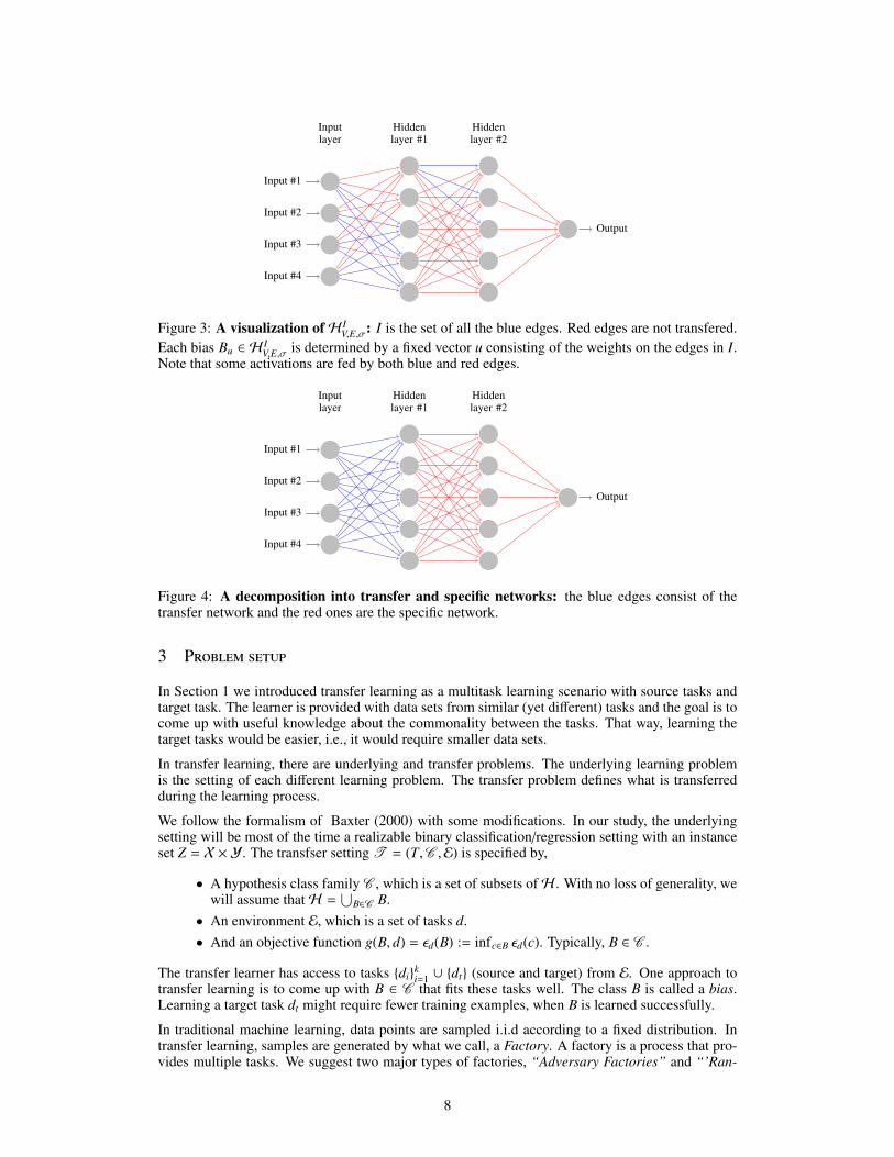
Figure 3: A visualization ofH IV,E,σ: I is the set of all the blue edges. Red edges are not transfered.
Each bias Bu ∈ HIV,E,σ is determined by a fixed vector u consisting of the weights on the edges in I.
Note that some activations are fed by both blue and red edges.
Input #1
Input #2
Input #3
Input #4
Output
Hiddenlayer #1
Inputlayer
Hiddenlayer #2
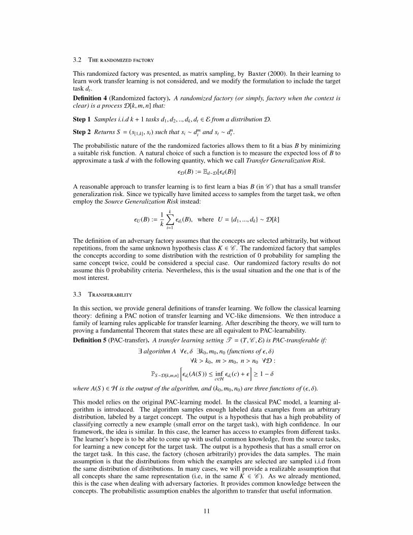
Figure 4: A decomposition into transfer and specific networks: the blue edges consist of thetransfer network and the red ones are the specific network.
3 Problem setup
In Section 1 we introduced transfer learning as a multitask learning scenario with source tasks andtarget task. The learner is provided with data sets from similar (yet different) tasks and the goal is tocome up with useful knowledge about the commonality between the tasks. That way, learning thetarget tasks would be easier, i.e., it would require smaller data sets.
In transfer learning, there are underlying and transfer problems. The underlying learning problemis the setting of each different learning problem. The transfer problem defines what is transferredduring the learning process.
We follow the formalism of Baxter (2000) with some modifications. In our study, the underlyingsetting will be most of the time a realizable binary classification/regression setting with an instanceset Z = X ×Y. The transfser setting T = (T,C ,E) is specified by,
• A hypothesis class family C , which is a set of subsets ofH . With no loss of generality, wewill assume thatH =
⋃B∈C B.
• An environment E, which is a set of tasks d.• And an objective function g(B, d) = εd(B) := infc∈B εd(c). Typically, B ∈ C .
The transfer learner has access to tasks diki=1 ∪ dt (source and target) from E. One approach to
transfer learning is to come up with B ∈ C that fits these tasks well. The class B is called a bias.Learning a target task dt might require fewer training examples, when B is learned successfully.
In traditional machine learning, data points are sampled i.i.d according to a fixed distribution. Intransfer learning, samples are generated by what we call, a Factory. A factory is a process that pro-vides multiple tasks. We suggest two major types of factories, “Adversary Factories” and “’Ran-
8

Factory
## (( ++ ,,d1
"" (( ++
d2 d3 ... dk dt
'' )) ,,z11 z1
2 z13 ... z1
m ... zt1 zt
2 zt3 ... zt
n
Figure 5: A factory: the sampling of samples zij from tasks di
ki=1∪dt. First, the tasks are selected
either arbitrarily or randomly (depending on the factory type). The sample sets si = zij are then
drawn from the corresponding tasks.
domized Factories”. The first generates supervised tasks (i.e, distributions over Z = X ×Y). Itselects concepts ci
ki=1 ∪ ct almost arbitrarily along to distributions over X. The other selects the
tasks randomly i.i.d from a distribution. In Section 4, we make use of adversary factories, while inSection 5 and Section 6 we use randomized factories instead.
In both cases, Figure 5 demonstrates the process done by the factory in order to sample training datasets. The difference between the two types arises from the method used to select the tasks.
3.1 The adversary factory
A factory selects k source tasks and a target task that the learner is tested on. An adversary factoryis a type of factory that selects supervised tasks (i.e, distributions over Z = X ×Y). It selects sourceconcepts ci
ki=1 that differ from the target concept ct and are otherwise chosen arbitrarily. The factory
also samples i.i.d distributions over X, piki=1 ∪ pt, from the distribution of distributionsD. By the
supervised behaviour of the learning setting, we have E = H × E′ where E′ is a set of distributionsover X.Definition 3 (Adversary factory). A factoryD[k,m, n] is a process with parameters [k,m, n] that:
Step 1 Selects k + 1 tasks d1, ..., dk, dt such that di = (pi, ci) ∈ E in the following manner,
• Samples i.i.d k + 1 distributions p1, p2, .., pk, pt from a distribution of distributionsD.• Selects any k source concepts c1, c2, .., ck and one target concept ct out ofH such that∀i ∈ [k] : ci , ct.
Step 2 Returns S = (s[1,k], st) such that si ∼ dmi and st ∼ dn
t .
Notation wise, if n = 0, we will write D[k,m] instead of D[k,m, 0] . When m = n = 0, we willsimply write D[k]. To avoid symbol overload, similar notions will be used to denote randomizedfactories, depending on the section. For a data set S sampled according to an adversary factory,we denote with O = (o1, ..., ok, ot) the original data set without the labels. This data set is a sampleaccording to oi ∼ pm
i and ot ∼ pnt where p1, ..., pk, pt ∼ D
k+1. In Section 4, all factories are adversary,while in the following sections they are randomized.
A K-factory is a factory that selects all concepts from K ∈ C . K is said to be the subject of thefactory. In this paper, we assume that all adversary factories are K-factories for some unknown biasK ∈ C . The symbol K will be preserved to denote the subject a factory.
We will often write, in Section 4 and the associated proofs, S ∼ D[k,m, n]. This is a slight abuse ofnotation since the concepts are not samples. It would mean that the claim is true for any selection ofthe concepts. In some sense, we can assume that there is an underlying unknown arbitrary selectionof concepts, and the data is sampled with respect to them. To avoid overload of notations, we willwrite O ∼ D[k,m, n] to denote the corresponding unlabeled data set version of S .
The requirement that ct differs from ci for all i ∈ [k] is essential to this first model. Intuitively,the interesting cases are those in which the target concept was not encountered in the source tasks.
9

Formally, it is easy to handle transfer learning using any learning algorithm, by just ignoring thesource data. In the other direction, if we allow repeated use of the target concept, then any transferalgorithm can be used for conventional learning by repeatedly using the target data as the source.Thus, without the requirement, one cannot get meaningful transfer learning statements for adversaryfactories.
The knowledge that a set of tasks was selected from the same K ∈ C , which is the subject of aK-factory, is the main source of knowledge made available during transfer learning. The secondtype of information arising from transfer learning is that all k + 1 distributions were sampled fromD.
Using the face recognition example, there is the set of visual concepts Bi,1 that captures the appear-ances of different furniture, and there is the set of visual concepts Bi,2 that capture the characteristicsof individual grasshoppers. From the source tasks, we infer that the target concept ct belongs to aclass of visual representations Bi,3 that contains image classifiers that are appropriate for modelingindividual human faces.
For concreteness, we present our running example. A disk in R3 around 0 is a binary classifier thathas radius r and a hyperplane h and is defined as follows:
fr,h(x) =
1 if x ∈ h ∩ B(r)0 if o.w
Here, B(r) is the ball of radius r around 0 in R3: B(r) = x ∈ R3 : ||x|| ≤ r. We define Eh = fr,h :r ≥ 0, where, C = Eh : ∀h hyperplane in R3 around 0. The following example demonstrates aspecific K-factory on the hypothesis class defined above.Example 1. We consider a K-factory as follows: 1. the disks are selected arbitrarily with thesame K such that the source concepts differ from the target concept, 2. D is supported with 3-Dmultivariate Gaussians with mean µ = 0 and covariance C = σ2I, where σ is sampled uniformly in[1, 5].
Compatibility between biases In the adversary model, the source and target concepts are selectedarbitrarily from a subject bias K ∈ C . Therefore, we expect the ability of a bias B to approximate Kto be the worst case approximation of a concept from K using a concept from B. Next, we formalizethis relation that we call “compatibility”.
We start with the mutual error rate, which is measured by εp(c1, c2) := εd(c1), where d = (p, c2).A bias B would be highly compatible with the factory’s subject K if for every selection of a targetconcept from K, there is a good candidate in B. The compatibility of a bias B with respect to thesubject K given an underlying distribution p over the instances setX is, therefore, defined as follows:
Compatibility Error Rate = errp(B,K) := supc2∈K
infc1∈B
εp(c1, c2)
In the adversary model, the distributions for the tasks are drawn from the same distribution of distri-butions. We, therefore, measure the generalization risk in the following manner:
Generalization Compatibility Error Rate = E(B,K) = Ep∼D
[errp(B,K)
]The empirical counterparts of these definitions are given, for an unlabeled dataset o drawn from thedistribution p as:
Empirical Compatibility Error Rate = erro(B,K) = supc2∈K
infc1∈B
εo(c1, c2)
where
Empirical Mutual Error Rate = εo(c1, c2) :=1|o|
∑x∈o
`(c2, c1(x))
In order to estimate E(B,K), the average of multiple compatibility error rates is used. A set ofunlabeled data sets O = (o1, ..., ok) is introduced, each corresponding to a different source task, andthe empirical compatibility error corresponding to the source data is measured by:
Source Empirical Compatibility Error Rate = EO(B,K) =1k
k∑i=1
erroi (B,K)
10
3.2 The randomized factory
This randomized factory was presented, as matrix sampling, by Baxter (2000). In their learning tolearn work transfer learning is not considered, and we modify the formulation to include the targettask dt.Definition 4 (Randomized factory). A randomized factory (or simply, factory when the context isclear) is a processD[k,m, n] that:
Step 1 Samples i.i.d k + 1 tasks d1, d2, .., dk, dt ∈ E from a distributionD.
Step 2 Returns S = (s[1,k], st) such that si ∼ dmi and st ∼ dn
t .
The probabilistic nature of the the randomized factories allows them to fit a bias B by minimizinga suitable risk function. A natural choice of such a function is to measure the expected loss of B toapproximate a task d with the following quantity, which we call Transfer Generalization Risk.
εD(B) := Ed∼D[εd(B)]
A reasonable approach to transfer learning is to first learn a bias B (in C ) that has a small transfergeneralization risk. Since we typically have limited access to samples from the target task, we oftenemploy the Source Generalization Risk instead:
εU(B) :=1k
k∑i=1
εdi (B), where U = d1, ..., dk ∼ D[k]
The definition of an adversary factory assumes that the concepts are selected arbitrarily, but withoutrepetitions, from the same unknown hypothesis class K ∈ C . The randomized factory that samplesthe concepts according to some distribution with the restriction of 0 probability for sampling thesame concept twice, could be considered a special case. Our randomized factory results do notassume this 0 probability criteria. Nevertheless, this is the usual situation and the one that is of themost interest.
3.3 Transferability
In this section, we provide general definitions of transfer learning. We follow the classical learningtheory: defining a PAC notion of transfer learning and VC-like dimensions. We then introduce afamily of learning rules applicable for transfer learning. After describing the theory, we will turn toproving a fundamental Theorem that states these are all equivalent to PAC-learnability.Definition 5 (PAC-transfer). A transfer learning setting T = (T,C ,E) is PAC-transferable if:
∃ algorithm A ∀ε, δ ∃k0,m0, n0 (functions of ε, δ)∀k > k0, m > m0, n > n0 ∀D :
PS∼D[k,m,n]
[εdt (A(S )) ≤ inf
c∈Hεdt (c) + ε
]≥ 1 − δ
where A(S ) ∈ H is the output of the algorithm, and (k0,m0, n0) are three functions of (ε, δ).
This model relies on the original PAC-learning model. In the classical PAC model, a learning al-gorithm is introduced. The algorithm samples enough labeled data examples from an arbitrarydistribution, labeled by a target concept. The output is a hypothesis that has a high probability ofclassifying correctly a new example (small error on the target task), with high confidence. In ourframework, the idea is similar. In this case, the learner has access to examples from different tasks.The learner’s hope is to be able to come up with useful common knowledge, from the source tasks,for learning a new concept for the target task. The output is a hypothesis that has a small error onthe target task. In this case, the factory (chosen arbitrarily) provides the data samples. The mainassumption is that the distributions from which the examples are selected are sampled i.i.d fromthe same distribution of distributions. In many cases, we will provide a realizable assumption thatall concepts share the same representation (i.e, in the same K ∈ C ). As we already mentioned,this is the case when dealing with adversary factories. It provides common knowledge between theconcepts. The probabilistic assumption enables the algorithm to transfer that useful information.
11

Next, we define VC-like dimensions for factory-based transfer learning. Unlike conventional VCdimensions, which are purely combinatorial, the suggested dimensions are algorithmic and proba-bilistic. This is because the post-transfer learning problem relies on information gained from thesource samples.
Definition 6 (Transfer VC dimension). T = (T,C ,E) has transfer VC dimension ≤ vc if:
∃ algorithm N ∀ε, δ ∃k0,m0 (functions of ε, δ) ∀k > k0, m > m0 ∀D :
PS∼D[k,m]
[vc(N(S )) ≤ vc and inf
c∈N(S )εdt (c) ≤ inf
c∈Hεdt (c) + ε
]≥ 1 − δ
Here, N(S ) ∈ C is a hypothesis class. We say that the transfer VC dimension is exactly d, if theabove expression does not hold with d replaced with vc − 1.
The algorithm N is called narrowing. These algorithms are special examples of how the commonknowledge might be extracted. In the first stage the algorithm, that is provided with source datareturns a narrow hypothesis class N(S ) that with a high probability approximates very well on dt.N(S ) can be viewed as a learned representation of the tasks from D. Post-transfer, learning takesplace in N(S ), where there exists a hypothesis that is ε-close to the best approximation possiblein H . In different situations, we will assume realizability, i.e, there exists B ∈ C such that D issupported by tasks d that satisfy infc∈B εd(c) = 0. In the adversary case, each factory is a K-factoryand, in particular, realizable.
In the face recognition example, the deep learning algorithm has access to face images of multiplehumans. From this set of images, a representation of an image of human faces is learned. Next,given the representation of human faces, the learner selects a concept that best fits the target data inorder to learn the specified human face.
By virtue of general VC theory, for learning a target task, with enough target examples (w.r.t. thecapacity of N(S ) instead of H’s capacity), one is able to output a hypothesis that is (ε + ε′)-closeto the best approximation in H , where ε′ is the accuracy parameter of the post-transfer learningalgorithm.
We, therefore, define a 2-step program. The first step applies narrowing and replacesH by a simpli-fied hypothesis class B = N(s[1,k]). The second step learns the target concept within B. An immediatespecial case, the T-ERM learning rule (transfer empirical risk minimization), uses an ERM rule asits second step. Put differently,
Input: S = (s[1,k], st).Output: concept cout such that εdt (cout) ≤ ε with probability ≥ 1 − δ.Narrowing narrow the hypothesis classH 7→ B := N(s[1,k]);Output cout = ERMB(st);
Algorithm 1: T-ERM learning rule
In the following sections, when needed, we will use the following to denote the minimal targetsample complexity of 2-step programs with n2step (a function of ε, δ).
We claim that whenever T is a learnable binary classification learning setting, once the narrowing isperformed, the ERM step is possible, with a number of samples that depend only on ε, δ. For thispurpose, the following Lemma is useful:
Lemma 1. The sample complexity of any learnable binary classification hypothesis classH of VCdimension u, is bounded by a universal function Nu(ε, δ). i.e, it depends only on the VC dimension.
Proof. Simply by Theorem 1.
Based on Lemma 1, with enough k,m (sufficient to apply the narrowing with error and confidenceparameters ε/2, δ/2) and n = Nu(ε/2, δ/2) from Lemma 1, the T-ERM rule returns a concept thathas error ≤ ε with probability ≥ 1 − δ.
12
4 Results in the adversary model
In this section, we make use of the adversary factories in order to present the equivalence betweenthe different definitions of transferability discussed above for the binary case. Furthermore, it isshown that in this case, transferability is equivalent to PAC-learnability. In the next section, westudy the advantages of transfer learning that exist despite this equivalence.
4.1 Transferability vs. learnability
The binary classification case
Theorem 3. Let T = (T,C ,E) be a binary classification transfer learning setting. The followingconditions on T are then equivalent:
1. Has finite transfer dimension.
2. Is PAC-transferable.
3. Is PAC-learnable.
Next, we provide bounds on the target sample complexity of 2-step programs.
Corollary 1 (Quantitative results). When T = (T,C ,E) is a binary classification transfer learningsetting that has transfer VC dimension vc, then the following holds:
C1 ·
(vc + log(1/δ)
ε
)≤ n2step(ε, δ) ≤ C2 ·
(vc + log(1/δ)
ε2
)For some constants C1,C2 > 0.
Proof. This corollary follows immediately from the characterization above and is based on Blumeret al. (1989). We apply narrowing in order to narrow the class to VC dimension ≤ v. The second steplearns the hypothesis in the narrow subclass. The upper bound follows when the narrow subclassdiffers from K (unrealizable case) while the lower bound turns in when K equals the narrow subclass(realizable case).
The regression case We demonstrate that transferability does not imply PAC-learnability in re-gression problems. PAC-learning and PAC-transferability are well defined for regression using ap-propriate losses. As the following Lemma shows, in the regression case, there is no simple equiva-lence between PAC-transferability and learnability.
Lemma 2. There is a transfer learning setting T = (T,C ,E) that is PAC-transferable but notPAC-learnable with squared loss `.
While the example in the proof of Lemma 2 (Appendix) is seemingly pathological, the scenarioof non-learnability in regression is common, for example, due to colinearity that gives rise to ill-conditioned learning problems. Having the ability to learn from source tasks reduces the ambiguity.
4.2 Trivial and non-trivial transfer learning
Transfer learning would be beneficial if it reduces the required target sample complexities. Wecall this the “non-trivial transfer” property. It can also be said that a transfer learning setting T =(T,C ,E) is non-trivial transferable, if there is a transfer learning algorithm for it with a target samplecomplexity smaller than the sample complexity of any learning algorithm of H by a factor 0 <c < 1. An alternative definition (that is not equivalent) is saying that the VC transfer and regularVC dimensions differ. We next describe a pathological case in which transfer is trivial, and thendemonstrate the existence of non-trivial transfer.
The pathological case can be demonstrated in the following simple example. Let H be the set ofall 2D disks in R3 around 0. Each Eh contains the disks on the same hyperplane h, for a finitecollection of h. Consider the factory D that samples distributions d supported only by points from
13

the hyperplanes h with a distance of at least 1 from the origin. Since, in our model, the conceptsare selected arbitrarily, consider the case where all source concepts are disks with a radius smallerthan 1, and the target concept has a radius of 2. In the source data, all examples are negative, and noinformation is gained on the hyperplane h.
Despite the existence of the pathological case above, the following Lemma claims the existence ofnon-trivial transferability.
Lemma 3. There exists a binary classification transfer learning setting T = (T,C ,E) (i.e, T is abinary classification setting) that is non-trivial transferable.
4.3 Generalization bounds for adversary transfer learning
In the previous section, we investigated the relationship between learnability and transferability. Itwas demonstrated that, in some cases, there is non-trivial transferability. In such cases, transferlearning is beneficial and helps to reduce the size of the target data.
In this section, we extend the discussion on non-trivial transferability. We focus on generalizationbounds for transfer learning in the adversary model. Two bounds are presented. The first boundis a VC-style bound. The second bound combines both PAC-Bayesian and VC perspectives. Theproposed bounds will shed some light about representation learning and transfer learning in general.Nevertheless, despite the wide applicability of these generalization bounds, it will not be trivial toderive a transfer learning algorithm from them since they measure the difference between general-ization and empirical compatibility error rates. In general, computing the empirical compatibilityerror rate requires knowledge about the subject of the factory, which is kept unknown. Therefore,without additional assumptions it is intractable to compute this quantity.
VC-style bounds for adversary transfer learning We extend the original VC generalizationbound for the case of adversary transfer learning. We call the presented bound, “The min-max trans-fer learning bound”. In this context, the min-max stands for the competition between the difficultyto approximate K and the ability of a bias B to approximate it.
This bound estimates the expected worst case difference between the generalization compatibilityof B to K and the empirical source compatiblity of B and K. The upper bound is the sum of tworegularization terms. The first penalizes both complexities of B and K with respect to the number ofsamples per task, m. The second penalizes on the complexity of C with respect to k.
The first step towards constructing a VC bound in the adversary model is defining a growth functionspecialized for this setting. The motivation is controlling the compatiblity between a bias B and thesubject K. Throughout the construction of compatibility measurements, the most elementary unit isthe empirical error of B, minc1∈B εo(c1, c2) for some c2 ∈ K along to an unlabeled data set o. Insteadof dealing with the whole bias B, we can focus only on c1 = ERMB(c2(o)). In that way we cancontrol the compatibility of B with K on the data set o. In transfer learning, we wish to controlthe joint error. Put differently, in the average of multiple compatibility errors on different data sets.For this purpose, we count the number of different configurations of two concepts ci,1 and ci,2 onunlabeled data sets oi such that ci,1 = ERMB(ci,2(oi)).
To avoid notaional overload, we assume that the ERM is fixed, i.e., we assume an inner imple-mentation of an ERM rule that takes a data set and returns a hypothesis for any selected bias B.Nevertheless, we do not restrict how it is implemented. More formally, ERMB(s) represents a spe-cific function that takes B, s and returns a hypothesis in B.
Based on this background, we denote the following set of configurations:
[H ,C ,K]O = (c1,1(o1), c1,2(o1), ..., ck,1(ok), ck,2(ok)) : ci,2 ∈ K and ci,1 = ERMB(ci,2(oi)) s.t B ∈ C
In addition, the Adversarial Transfer Growth Function τ(k,m; C ,K),
τ(k,m; C ,K) = maxO∈Xmk
∣∣∣∣[H ,C ,K]O
∣∣∣∣This quantity represents the worst case number of optional configurations.
14

Theorem 4 (The min-max transfer learning bound). Let T = (T,C ,E) be a binary classificationtransfer learning setting. Then,
∀D ∀K ∈ C :EO∼D[k,m]
[supB∈C
∣∣∣∣E(B,K) − EO(B,K)∣∣∣∣]
≤4 +
√log(τ(2k,m; C ,K))√
2k+
4 +√
log(supB τB(2m)) + log(τK(2m))√
2m
PAC-Bayes bounds for adversary transfer learning This bound combines between PAC-Bayesian and VC perspectives. We call it “The perturbed min-max transfer learning bound”. This isbecause there is still a competition between the ability of the bias to approximate and the difficultyof the subject. Nevertheless, in this case the bias is perturbed.
We take a statistical relaxation of the standard model. A set of posterior distributions Q and a priordistribution P, both over C are taken. Extending the discussion in Section 2, the aim is being able toselect Q ∈ Q that best fit the data instead of a concrete bias. In this setting, we measure an expectedversion of the generalization compatibility error rate with B distributed by Q ∈ Q. We call it theExpected Generalization Compatibility Error Rate. Formally,
E(Q,K) = EB∼QEp∼D
[errp(B,K)
]It is important to note that the left hand side of the bound is, in general, intractable to compute. Thisis due to its direct dependence on K which is unknown. Nevertheless, there still might be conditionsin which different learning methods do minimize this argument. In addition, it gives insights onwhat a “good” bias is.
Theorem 5 (The perturbed min-max transfer learning bound). Let T = (T,C ,E) be a binaryclassification transfer learning setting. In addition, P a prior distribution andQ a family of posteriordistributions, both over C . Let δ ∈ (0, 1) and λ > 0, then for all factoriesD with probability ≥ 1− δover the selection of O ∼ D[k,m],
∀Q ∈ Q,K ∈ C : E(Q,K) ≤1k
k∑i=1
EB∼Q[erroi (B,K)]
+
√2 log(τH (2m)) + log(8/λδ)
m+
1m
+
√KL(Q||P) + log(2k/δ)
2(k − 1)+ λδ
With the restriction that k ≥ 8 log( 2δ )
(λδ)2 .
5 Results in the randomized model
We start our discussion of randomized factories with the following Lemma that revisits the disks inR3 example above for this case.
Lemma 4. Let T = (T,C ,E) be a realizable transfer learning setting such that H is the setof all 2D disks in R3 around 0. Each Eh = disks on the same hyperplane h and C = Eh :∀h hyperplane in R3 around 0. This hypothesis class has transfer VC dimension = 1 (and reg-ular VC dimension = 2).
5.1 Transferability vs. learnability
A transferring rule or bias learner N is a function that maps a source data (i.e, s[1,k]) into a bias B.An interesting special case is the simplifier. A simplifier fits B ∈ C that has a relatively small errorrate.
Definition 7 (Simplifier). Let T = (T,C ,E) be a transfer learning setting. An algorithm N withaccess to C is called a simplifier if:
∀ε, δ ∃k0,m0 (functions of ε, δ) ∀k > k0, m > m0 ∀D :
PS
[εD(N(S )) ≤ inf
B∈CεD(B) + ε
]≥ 1 − δ
15

Here, the source data S is sampled according to D[k,m]. In addition, N(S ) ∈ C , which is ahypothesis class, is the result of applying the algorithm to the source data. The quantities k0,m0 arefunctions of ε, δ.
The standard ERM rule is next extended into a transferring rule. This rule returns a bias B that hasthe minimum error rate on the data, measured for each data set separately. This transferring rule,called C − ERMC (S ) is defined as follows,
C − ERMC (S ) := arg minB∈C
1k
k∑i=1
εsi (c∗i,B), s.t c∗i,B = ERMB(si)
This transferring rule was previously considered by Ando et al. (2005) who named it Joint ERM.
Uniform convergence (Shalev-shwartz et al. (2010)) is defined for every hypothesis class H (w.r.tloss `), in the usual manner:
∀d : PS∼dk
[∀c ∈ H :
∣∣∣∣εd(c) − εs(c)∣∣∣∣ ≤ ε] ≥ 1 − δ
It can also be defined for C (w.r.t loss g) as:
∀D : PU∼D[k]
[∀B ∈ C :
∣∣∣∣εD(B) − εU(B)∣∣∣∣ ≤ ε] ≥ 1 − δ
For any k larger than some function k(ε, δ).
The following lemma states that whenever bothH and C have uniform convergence properties, thenthe C-ERMC transferring rule is a simplifier forH .
Lemma 5. Let T = (T,C ,E) be a transfer learning setting. If both C and H have uniformconvergence properties, then the C − ERM rule is a simplifier ofH .
The preceeding Lemma explained that C − ERMC transferring rules are helpful for transferringknowledge efficiently.
The next Theorem states that even if the hypothesis classH has an infinite VC dimension, there stillmight be a simplifier outputing hypothesis classes with a finite VC dimension. This result, however,could not be obtained when restricting the size of the data to be bounded by some function of ε, δ.Therefore, in a sense, there is transferability beyond learnability.
Theorem 6. The following statements hold on binary classification.
• There is a binary classification transfer learning setting T = (T,C ,E) such thatH has aninfinite VC dimension, has a simplifier N that always outputs a finite VC dimensional biasB.
• If a binary classification transfer learning setting T = (T,C ,E) has an infinite VC dimen-sion, then supB∈C vc(B) = ∞.
5.2 Generalization bounds for randomized transfer learning
In the previous section, we explained that whenever bothH and C have uniform convergence prop-erties, there exists a simplifier for this transfer learning setting. We explained that, in this case, aC-ERM rule is an appropriate simplifier. In this section, we widen the discussion on the existenceof a simplifier for different cases. For this purpose, we extend famous generalization bounds fromstatistical learning theory to the case of transfer learning.
VC-style bounds for transfer learning We begin with an extension of the original VC bound(see Section 2) to the case of transfer learning. It upper bounds the expected (w.r.t random sourcedata) difference between the transfer generalization risk of B and the 2-step Source Empirical Riskworking on B. A mapping r : B 7→ rB from a bias B to a learning rule of the bias (i.e, outputshypotheses in B with empirical error that converge to infc∈B εd(c)) is called post transfer learning
16

rule/algorithm (see Equation 2). Informally, the 2-step source empirical risk measures the empiricalsuccess rate of a post transfer learning rule on a few data sets. The bounding quantity depends onthe ability of the post transfer learning rule to generalize.
The 2-step source empirical risk is formally defined as follows,
εS (B, r) :=1k
k∑i=1
εsi (rB(si)), s.t S = s[1,k]
Next, the standard constructions of the original VC bound are extended,[H ,C , r
]S =
r1,B(s1), ..., rk,B(sk) : B ∈ C
, s.t S = s[1,k]
Here, ri,B := rB(si) denotes the application of the learning rule rB on si and ri,B(si), the realization ofri,B on si. The equivalent of the standard growth function in transfer learning is the transfer growthfunction,
τ(k,m, r) = maxS
∣∣∣∣[H ,C , r]S
∣∣∣∣With this formalism, we can state our extended version of the VC bound.
Theorem 7 (Transfer learning bound 1). Let T = (T,C ,E) be a binary classification transferlearning setting such that T is learnable. In addition, assume that r is a post transfer learning rule,i.e, endowed with the following property,
∀d, B : rB(·) ∈ B and Es∼dm
[∣∣∣∣infc∈B
εd(c) − εs(rB(s))∣∣∣∣] ≤ ε(m)→ 0 (2)
Then,
ES∼D[k,m]
[supB∈C
∣∣∣∣εD(B) − εS (B, r)∣∣∣∣] ≤ 4 +
√log(τ(2k,m, r))√
2k+ ε(m)
We conclude that in binary classification, if T is learnable, and r satisfies Equation 2 then, thereexists a simplifier whenever the transfer growth function τ(k,m, r) is polynomial in k.
PAC-Bayes bounds for transfer learning We provide two different PAC-Bayes bounds for trans-fer learning. The first bound estimates the gap between the generalization transfer risk of each B ∈ Cand the average of the empirical risks of c∗i,B in the binary classification case. On the other hand,Theorem 9 will argue a more general case when H might have an infinite VC dimension or theunderlying learning setting is not binary classification.
The first approach concentrates on model selection within PAC-Bayesian bounds. It presents abound for model selection that combines PAC-Bayes and VC bounds. We construct a generalizationbound to measure the fitting of a random representation. i.e, the motivation is searching for Q thatminimizes,
R(Q) = EB∼QEd∼D
[infc∈B
εd(c)]
Theorem 8 (Transfer learning bound 2). Let T = (T,C ,E) be a binary classification transferlearning setting. In addition, P a prior distribution and Q a family of posterior distributions, bothover C . Let δ ∈ (0, 1) and λ > 0, then with probability ≥ 1 − δ over S ,
∀Q ∈ Q : R(Q) ≤1k
k∑i=1
EB∼Q
[εsi (c
∗i,B)
]+
√log(τH (2m)) + log(8/λδ)
m+
1m
+
√KL(Q||P) + log(2k/δ)
2(k − 1)+ λδ
With the restriction that k ≥ 8 log(2/δ)(λδ)2 .
17

We then derive the following randomized transferring rule,
argminQ
1k
k∑i=1
EB∼Q
[εsi (c
∗i,B)
]+
√KL(Q||P) + log(2k/δ)
2(k − 1)
Which is helpful only when both k,m tend to increase.
The previous bound relied on the assumption that the learning setting is binary classification andthe underlying learning setting is learnable. Next, we suggest a different approach to PAC-Bayesbounds for transfer learning. The current bound is pure PAC-Bayesian and is more related to Pentina& Lampert (2014). In their work, the motivation is to be able to learn a prior distribution for learningnew tasks. The aim is measuring the effectiveness of a prior distribution for learning new tasks witha selected learning rule. The weakness in their analysis is that it relies on the assumption that thesource training data sets and the target training data set are i.i.d distributed and thus proportionalin their sizes. In this work, we suggest a different perspective for PAC-Bayes transfer bounds thatovercomes this problem.
The first step towards the construction of the bound is to adopt a generalized PAC-Bayesian setting.
• A transfer learning setting T = (T,C ,E).
• P a prior distribution and Q a family of posterior distributions, both over C .
• p a prior distribution and
U =
Qq(c) =
∫B
Q(B) · q(c; B) dB : Q ∈ Q, q
a family of posterior distributions, both overH .
The set U consists of all distributions that first sample a subset B from Q and then sample c fromq(·; B) that is over B. We are again interested in finding Q that minimizes,
R(Q) = EB∼QEd∼D
[infc∈B
εd(c)]
Theorem 9 (Transfer learning bound 3). Assume the PAC-Bayesian framework above. Let δ ∈ (0, 1)and λ > 0, then with probability ≥ 1 − δ over S ∼ D[k,m], the following holds for all Q ∈ Q,
R(Q) ≤1k
k∑i=1
minqiEc∼Qqi
[εsi (c)
]+
√KL(Qqi ||p) + log(2m/λδ)
2(m − 1)+
√KL(Q||P) + log(2k/δ)
2(k − 1)+ λδ
With the restriction that k ≥ 8 log(2/δ)(λδ)2 .
As for the previous bound, we can arrive to a different transferring rule,
argminQ
1k
k∑i=1
minqiEc∼Qqi
[εsi (c)
]+
√KL(Qqi ||p) + log(2m/λδ)
2(m − 1)
+
√KL(Q||P) + log(2k/δ)
2(k − 1)
6 Deep transfer learning
6.1 VC-style bounds for deep transfer learning
It is interesting to show how Theorem 7 can be applied to the case of deep learning. We provide aVC-like bound for deep learning. This will be a major step towards proving nontrivial transferabilityfor a very wide class of neural network architectures. In addition, it will give insights on major open
18

questions like “deep architectures vs. shallow architectures”, “expressivity of deep architectures”and “generalization ability of deep architectures” in their general aspect and in the particular case oftransfer learning.
We study the case when the architecture decomposes into transfer and specific architecturesHt andHu (see Section 2). For each bias B, we denote its corresponding neural network with hB.
First, we show that the growth function of the transfer learning setting can be bounded with thegrowth function ofHt. Denote τt(·) the growth function of the hypothesis classHt.
We assume that the produced labels of a post transfer learning rule r are independent of B and sgiven hB(s). i.e,
rB1 (s1)(s1) = rB2 (s2)(s2) whenever hB1 (s1) = hB2 (s2) (3)It can also be stated that, if rB1 (s1) and rB2 (s2) are trained hypotheses under the assumption thathB1 (s1) = hB2 (s2), then their labelings on s1 and s2 are the same. We will next show that thisassumption is common when the hypothesis class can be decomposed toHu Ht.
Lemma 6. Let T = (T,H IV,E,sign,E) be a transfer learning setting such that T = (HV,E,sign,Z, `) and
` is the 0-1 loss. Assume that I consists of all edges between the first j layers. Let r be any posttransfer learning rule (i.e, a mapping r : B → rB such that rB(s) ∈ B for all finite s ⊂ Z) satisfying3. Then,
τ(k,m, r) ≤ τt(mk) ≤ (mke)|I|
Where τt is the growth function of the hypothesis classHt.
Plug in Lemma 6 into Theorem 7 for the proposed deep learning setting and arrive at the followinggeneralization bound.
Theorem 10 (Deep learning bound 1). Let T = (T,H IV,E,sign,E) be a transfer learning setting such
that T = (HV,E,sign,Z, `) and ` is the 0-1 loss. In addition, assume that r satisfies Equation 3 andEquation 2. Then,
ES∼D[k,m]
[supB∈C
∣∣∣∣εD(B) − εS (B, r)∣∣∣∣] ≤ 4 +
√|I| log(mke)√
2k+ ε(m)
Proof. An application of Theorem 7 for the discussed case with the bound from Lemma 6.
Theorem 11 (Deep learning bound 2). Let T = (T,H IV,E,sign,E) be a transfer learning setting such
that T = (HV,E,sign,Z, `), ` is the 0-1 loss and denote E = I ∪ J (where I ∩ J = ∅). In addition,assume that r : B→ ERMHu (hB(·)) hB. Then,
ES∼D[k,m]
[supB∈C
∣∣∣∣εD(B) − εS (B, r)∣∣∣∣] ≤ 4 +
√|I| log(mke)√
2k+
8 +√
4|J| log(2me)√
2mWhere rB := ERMHu (hB(·))hB is a learning rule that takes a data set s and outputs ERMHu (hB(s))hB in return.
This Theorem asserts that nontrivial transferability holds among a very general class of transferlearning settings of neural networks. As we have shown, whenever the architecture is divided intotransfer and specific parts, a narrowing process reduces the whole hypothesis class of neural net-works into one that has lower capacity. In a realizable case (i.e, there is B such that for all d we haveinfc∈B εd(c) = 0), the transfer VC dimension might decrease.
6.2 PAC-Bayes bounds in deep transfer learning
We next apply the PAC-Bayesian bounds of Section 5.2 to the case of neural networks.
The motivation is transferring common weights between neural networks. It is preferable to useH I
V,E,σ as the hypothesis class family. Inspired by the Gaussian parameterization for neural networkspresented by McAllester (2013), a bias corresponding to weight vector u is identified with a Gaussiandistribution centered by u. Formally,
Qu ∼ N(u, 1), P ∼ N(0|I|, 1) and Q =Qu | u ∈ R|I|
=⇒ KL(Qu||P) = ||u||2/2 (4)
19
Where 0|I| is a (|I|-dimensional) vector of zeros and 1 is a unit matrix (of dimension |I| × |I|).
Theorem 12 (Deep learning bound 3). Let T = (T,C ,E) be a transfer learning setting such thatH := HV,E,sign and C := H I
V,E,sign for any neural network architecture (V, E, σ) and I ⊂ E. P and Qas above. Let δ ∈ (0, 1) and ε > 0, then with probability ≥ 1 − δ over S , for all u,
R(Qu) ≤1k
k∑i=1
EB∼Qu
[εsi (c
∗i,B)
]+
√|E| log(2me) + log(8/ε)
m+
1m
+
√||u||2/2 + log(2k/δ)
2(k − 1)+ ε
With the restrictions that k ≥ 8 log(2/δ)ε2 .
Proof. An application of Theorem 8 with the explanations above and λδ = ε.
Post transfer (after selecting B := B∗ that best fits the data), one is able to use the common knowledgeextracted in the transfer step in order to learn a new concept. One approach to do it is by fixing I’thweights to be B∗’s and learning only the rest of the weights. Formally, we learn the target taskwithin the hypothesis class B∗ that consists of all neural networks with architecture (V, E, sign) andI’s weights are B∗’s vector.
Lemma 7. The VC dimension of each B ∈ H IV,E,sign is vc(B) = O
(|J| log |J|
).
Following the same line, we apply Theorem 9 with Gaussian distributions. As before, each bias Bu isidentified with a Gaussian distribution centered by u. In addition, a neural network hV,E,sign,w ∈ Bu, isidentified with the weight vector w = u||v (concatenation of two vectors) consisting of all the weightson E. We fit a Gaussian distribution centered by this weights vector to parameterize hV,E,sign,w. Weselect,
Q =Qu ∼ N(u,1) : u ∈ R|I|
, P ∼ N(0|I|,1)
=⇒ KL(Qu||P) = ||u||2/2And,
U =Qu,v ∼ N(u, 1) · N(v,1) : u ∈ R|I|, v ∈ R|J|
, p ∼ N(0|E|,1)
=⇒ KL(Qu,v||p) = ||u||2/2 + ||v||2/2Theorem 13 (Deep learning bound 4). Let T = (T,C ,E) be a transfer learning setting such thatH := HV,E,sign and C := H I
V,E,sign for any neural network architecture (V, E, σ) and I ⊂ E. P, Q, pandU as above. Let δ ∈ (0, 1) and ε > 0, then with probability ≥ 1 − δ over S , for all u,
R(Qu) ≤1k
k∑i=1
minviEc∼Qu,vi
[εsi (c)
]+
√||u||2/2 + ||vi||
2/2 + log(2m/ε)2(m − 1)
+
√||u||2/2 + log(2k/δ)
2(k − 1)+ ε
With the restriction that k ≥ 8 log(2/δ)ε2 .
Proof. An application of Theorem 9 with the explanations above and λδ = ε.
6.3 Tradeoffs and practical recommendations
The proposed generalization bounds give worst case estimations of the generalization risk throughdifferent approaches. They are helpful in finding connections between the involved complexities ofthe network and the size of data. This raises several acute tradeoffs that are worth explaining. Wederive different tradeoffs that occur under alternative assumptions on the involved parameters.
Many of the tradeoffs include big O notations. The following bound is often applied in order toderive sufficient conditions for the relevant quantities:
∀a ≥ 1, b > 0 : x ≥ 4a log(2a) + 2b⇒ x ≥ a log(x) + b (5)
20

Tradeoff between k and m Refering to Theorem 11. Assume that the total number of sourcesamples mk = M is fixed. An interesting question is how many samples to invest in each task (i.e,what is the best m).
With no loss of generality, we assume that 8 ≤√
4|J| log(2me) and 4 ≤√|I| log(mke). We are
interested in bounding the regularization terms with ε,√2|I| log(mke)
k≤ ε,
√8|J| log(2me)
m≤ ε
By Equation 5, we derive a sufficient condition,
m = Θ
(|J| log(|J|/ε)
ε2
)and k = Θ
(|I| log(|I| · |J|/ε)
ε2
)Therefore,
m ≈ Θ
√
M|J| log(|J|)|I| log(|I| · |J|)
and k ≈ Θ
√
M|I| log(|I| · |J|)|J| log(|J|)
(Neglecting constants and log(1/ε)).
The need to increase k as a function of m Refering to Theorem 11. It is very natural to believethat whenever m increases, k should also increase. That is because, a selection of B that dependsonly on very accurate information of k fixed number of tasks is biased. The selected B would fitvery well with those tasks but might fail to fit with unseen different tasks. This is an overfitting thatmight occur only in the case of transfer learning. We would like to measure how much is sufficientto increase k as a function of m in order to avoid overfitting. According to Theorem 10, if we fixall of the parameters except m, it is required to take k = Ω(log(m)) in order to avoid the discussedoverfitting. Therefore, the transferring rule arg minB εS (B, r) overfits w.r.t tasks if k is smaller byorders of magnitude than log(m). This is a desireable situation since in most practical situations k isnot tiny w.r.t m.
In the other direction, it does not seem there is dependence between k,m that requires m to increasewhenever k does.
Tradeoff between m, k and the capacity of the specific part |J| Refering to Theorem 11. Thecapacity of the specific architecture Hu is measured by |J|. The VC dimension of Hu depends onlyon that capacity, i.e, vc(Hu) = O(|J| log |J|). From the bound, we adress that m = Θ(|J| log |J|)is sufficient in order to overcome the size of the specific architecture. In addition, it seems thatthe dependence of k on |J| is much weaker. In the previous tradeoff, the dependence of k on mis logarithmic, i.e, it is required to take k = Ω(log(m)) in order to avoid overfitting. Therefore,in the case where m and k are chosen wisely (satisfying m = Θ(|J| log |J|) and k = Ω(log(m)))then k = Ω(log log |J|). A Larger m is required in order to train the specific part of each networkseparately.
Tradeoff between k and the capacity of the transfer |I| Refering to Theorem 11. As before,we arrive at k = Θ(|I| log |I|) is sufficient in order to overcome the size of the transfer architecture.The combination of this argument and the very weak dependence of k on |J| raises the insight thatlarger k are required mostly to overcome the capacity of the transfer (i.e, |I|). Larger k is requiredto overcome the common transfer architecture. It can also be said that k depends on the whole sizeof the architecture, but it has a much stronger dependence on the capacity of the transfer despite thespecific part.
Tradeoff between k and the number of target samples n By the fundamental Theorem of learn-ability Vapnik & Chervonenkis (1971), the sample complexity (of a binary classification learningsetting) is Θ
(vc+log(1/δ)
ε2
). Therefore, in order to reduce n, it is necessary to decrease the VC dimen-
sion of the post transfer learning setting. By Lemma 7, we have target VC dimension O(|J| log |J|).Thus, it is desired to increase |I|. Nevetheless, by the conclusion of the last tradeoff, it will require kto grow linearly with |I| log |I|.
21

Transferring too much information hurts performance The richer the source data is, the moreinformation that can be transferred. Transferring too much information hurts performance. This canbe seen in the bottleneck effect demonstrated in Taigman et al. (2015), where creating a lower-dimrepresentation improves transfer performance. Bottleneck in the context of information theory wasinvestigated by Tishby et al. (2000), Tishby & Zaslavsky (2015).
We consider the case where J consists of the bottleneck weights (i.e, all weights between the repre-sentation layer and the output). In this case, post transfer, the size of target data required to obtainan error rate at most ε far from the optimum is n = Θ
(|J|+log(1/δ)
ε2
). Therefore, in order to control
the post transfer error rate, we have to require |J| = Θ(nε2) (neglecting log(1/δ)). The best possi-ble representation, that has the smallest transfer generalization risk, is the one of size equals to theexamples size. We are looking for a smaller representation that is still ε-close to the best possiblerepresentation. More formally, for any ε, there is an optimal size for the representation that has errorat most ε larger than the error of the best representation. The error of the bias learned in the transferstage depends on how far J of size Θ(nε2) is from optimal representation size.
Learning with noisy labels Refering to Theorem 11. The performance of Convnets to learn taskswith noisy labels was studied by Sukhbaatar & Fergus (2014). They showed that Convnets havegood performance in learning tasks even when the labels are noisy. They introduced an extra noiselayer that adapts the network to the noise distribution. The proposed factory framework can modelnoisy labels and shed light on this situation.
When learning with noisy labels, there is a target task d = (c∗, p). The goal is to learn c∗ through krandom noisy streams with “mean” d. We introduce a transfer learning setting T = (T,C ,E). Theunderlying learning task T = (H ,Z, `) is a supervised binary classification setting. The hypothesisclass is a neural networks architectureH := HV,E,sign. The environment is,
E =(c, p) | c is any function
The factory D is symmetric around (c∗, p) (i.e, the probability to sample (c1, p) is equal to theprobability to sample (c2, p) under the assumption that εd(c1) = εd(c2)).
In this setting, the learned common representation is the full neural network. It can also be said thatthe algorithm learns a neural network that fits best with random noisy streams. The hypothesis classfamily is C := H I
V,E,σ such that I = E, i.e,
C := HEV,E,σ =
hV,E,σ,w | w ∈ R|E|
This can be treated simply asHV,E,σ. Therefore, each hB (corresponding to bias B ∈ C ) is simply aneural network inH (i.e, a concept). In this case, the transfer risk is,
εD(c) = Eb∼D[εb(c)]
This quantity is minimized by any c such that the set x | c(x) , c∗(x) has probability 0 (w.r.t p).Any other function will not minimize this quantity. We apply Theorem 10 (see Appendix F) withHt := H (and Hu = ∅). In addition, |J| = 0 and |I| = |E|. Let cS = arg minc εS (c) = 1
k∑k
i=1 εsi (c),then with probability ≥ 1 − δ (over S ),
εD(cS ) ≤ infc∈H
εD(c) +8 +
√4|E| · log(2emk)
δ√
2k+
16
δ√
2m(6)
Therefore, the output cS converges to the best possible hypothesis as k,m tend to increase.
Accurately, it is sufficient to provide,
m = Θ
(1
(δε)2
)and k = Θ
(|E|
(δε)2 log(|E|δε
))In order to have, εD(cS ) ≤ infc∈H εD(c) + ε.
Therefore, the total number of samples sufficient to provide is Θ(|E|
(δε)4 log(|E|δε
)).
22

Comparing the binary classification bounds in Baxter (2000) with our VC bound Refering toTheorem 11. In the work of Baxter (2000), they construct multitask generalization bounds (boundson the source generalization risk for k specified tasks) for deep learning in the binary classificationcase. In their analysis, they fix k and conclude that the number of samples per task should be:
m = O(|H| log(1/ε)
ε2
)Where H ⊂ V is the set of hidden neurons.
On the other hand, with our analysis we arrived to m = O(|J| log(|J|/ε)
ε2
)(neglecting 1/δ in both calcu-
lations).
In most interesting cases, |J| log |J| |H| (see Taigman et al. (2014), Taigman et al. (2015), Donahueet al. (2013), Razavian et al. (2014)).
6.3.1 PAC-Bayes tradeoffs
The tradeoffs above were all derived based on the VC bound. Tradeoffs can also be derived from thePAC-Bayes bounds. The PAC-Bayes settings are more general, since arbitrary weights can be trans-fered, and not just parts of the architectures. This setting is also not limited to binary classification.
Tradeoff between m and the size of the architecture |E| Refering to Theorem 12. The KL(·||·)measures the difference between two distributions. There is a direct connection between the KL-divergence and the dimension of the space of the distributions. In the case we investigate, the priorand posterior distributions are Gaussian distributions. For instance, we can assume that the parame-ters uopt of the optimal posterior over biases, Qopt and vopt of the optimal posterior distributions overconcepts (for each task), qopt, were selected i.i.d from some distribution D and obtain,
Euopt ,vopt∼D|E| [KL(Qoptq ||p)] = A · |E|, s.t A := Ex∼D
[x2/2
]Requiring that the expected specific regularization term for the optimal posterior be at most ε withthe fact that E[
√X] ≤
√E[X] and the selection λδ = ε,
Euopt∼D|I|
√
KL(qopt ||p) + log(2m/λδ)2(m − 1)
≤√
A · |E| + log(2m/λδ)2(m − 1)
≤ ε
That simply concludes to,
m = Θ
A · |E| + log(
1ε
)ε2
(7)
Therefore, it is required to increase m linearly as |E| grows. On the other hand, from the bound itdoes not seem that there is such a strong dependence between k and |E|.
Tradeoff between k and the capacity of the transfer |I| Refering to Theorem 12 and Theorem 13.We use the same analysis as before. It is assumed that the parameters uopt of the optimal posteriordistribution, Qopt, were selected i.i.d from some distribution D. Thus,
Euopt∼D|I| [KL(Qopt ||P)] = A · |I|, s.t A := Ex∼D
[x2/2
]We refer
√KL(Q||P)+log(2k/δ)
2(k−1) as the transfer regularization term and would like to restrict it to be at
most ε for the optimal posterior. Using the fact that E[√
X] ≤√E[X],
Euopt∼D|I|
√
KL(Qopt ||P) + log(2k/δ)2(k − 1)
≤√
A · |I| + log(2k/δ)2(k − 1)
≤ ε
That simply concludes to,
k = Θ
A · |I| + log(
1δε
)ε2
(8)
Therefore, it is required to increase k linearly as |I| grows.
23

Tradeoff between k and m Assume that the total number of source samples mk = M is fixed. Weprovide an analysis, based on Theorem 13.
It is assumed that the parameters uopt and vopt of the optimal posterior distributions, Qopt and qopt,were selected i.i.d from some distribution D, we have:
Euopt∼D|I| [KL(Qopt ||P)] = Ex∼D
[x2/2
]· |I| := A · |I|
In addition,Euopt ,vopt∼D|E| [KL(qopt ||p)] = Ex∼D
[x2/2
]· |E| = A · |E|
In order to ensure that the expected regularization term for the optimal posterior will be at most ε bythe fact that E[
√X] ≤
√E[X] we may require
λ =ε
3δ,
√A · |E| + log(2m/λδ)
2(m − 1)≤ε
3and
√A · |I| + log(2k/δ)
2(k − 1)≤ε
3
Applying Equation 5 and neglecting log(1/δε),
m = Θ
(A · |E|ε2
)≈ Θ
√|E| · M|I|
and k = Θ
(A · |I|ε2
)≈ Θ
√|I| · M|E|
Comparing the regression bounds in Baxter (2000) with our PAC-Bayes bound Referingto Theorem 13. In the work of Baxter (2000), they construct transfer generalization bounds fordeep learning in regression settings. The bottom line of their analysis concludes that (neglectinglog(1/εδ)),
k = O(|E|/ε2
)and m = O
(|H|/ε2
)Where H ⊂ V is the set of hidden neurons.
On the other hand, neglecting log(1/εδ), with the analysis above we arrived at k = O(|I|/ε2
)and
m = O(|E|/ε2
). Therefore, our bound requires fewer number of multiple tasks but more samples per
task.
7 RelatedWork
The standard assumption in supervised machine learning algorithms is to have models trained andtested on samples drawn from the same probability distribution. Often, however, there are manylabeled training samples from a source task and the goal is to construct a learning rule that performswell on a target task with a different distribution and little labeled training data. This is the problemof Domain Adaptation (DA), where a successful scheme typically utilizes large unlabeled samplesfrom both tasks to adapt a source hypothesis to the target task. Kifer et al. (2004); Ben-Davidet al. (2007); Mansour et al. (2009a); Ben-David et al. (2010a) suggest adapting these tasks byconsidering the divergence between the source and target sources. Based on this divergence, theyprovide PAC-like generalization bounds. Alternatively, Li & Bilmes (2007) measure the adaptionusing divergence priors and learn a hypothesis for the target task by applying an ERM rule on thesource task. A different approach is due to Yang & Hospedales (2014). They coined a new termcalled semantic descriptors. These are generic descriptors uniform for a few tasks that reduce theuncertainty about the tasks. Hardness results for DA are explored in Ben-David et al. (2010b).
Our work does not assume that the tasks are comparable, e.g., by divergence of tasks. Our onlyrestriction is having enough data from a common source (the factory), similar to the original PACmodel. Two types of common sources are explored. The first is used to investigate the adversarysituations when the concepts are selected almost arbitrarily. The second, uses random concepts, andwas previouslty proposed by Baxter (2000) in the concept of inductive bias learning, in which thereis no one dedicated target task. Our random concept factory differs from that of Baxter (2000) inthat the transfer task might have considerably less training examples than the source tasks. We are,therefore, able to model the case in which the source tasks have practically unrestricted samples,while harvesting samples for the target task is much harder. We also discuss common aspects as
24

in Ando et al. (2005). Their work proposes the Joint ERM rule (which we redefine as the C-ERMrule). In our work, we extend the discussion on this transferring rule and suggest a regularizedrandom version of it derived from PAC-Bayesian bounds introduced in the paper.
Cortes et al. (2008); Crammer et al. (2008); Mansour et al. (2009b) combine several training sourcesto better describe the target distribution. It is assumed that the distribution of the target task is alinear combination (that sums to 1) of the source distributions. Our work differs from these works,since we do not seek to approximate the target distribution from the multiple sources, but rather totransfer a concept that facilitates learning from a few examples in the target task.
Transfer learning has attracted considerable recent attention, with the emergence of transfer learningin visual tasks Krizhevsky et al. (2012); Girshick et al. (2014); Fei-Fei et al. (2006); Yang et al.(2007); Orabona et al. (2009); Tommasi et al. (2010); Kuzborskij et al. (2013). In these contributions,the application of transfer learning is done without assuming any knowledge about the relatedness ofthe source and target distributions. Although this setting has been explored empirically with success,a formal theory of transfer learning is mostly missing.
Recently, the generalization properties of the transfer learning approach was investigated in Pentina& Lampert (2014); Kuzborskij & Orabona (2013); Tommasi et al. (2014). Specifically, Pentina& Lampert (2014) measure the representation transfer by PAC-Bayesian generalization. Their ap-proach assumes that the data set of the target task is proportional to each source data set. Al-ternatively, Kuzborskij & Orabona (2013); Tommasi et al. (2014) measure the amount of transferaccording to its stability with respect to the leave-one-out error Mukherjee et al. (2002),Bousquet& Elisseeff (2002). Our work differs from these works by its scope. We focus on presenting whentransfer learning is meaningful and how to measure its success when transferring a narrowed hy-pothesis class between source and target tasks. This process requires a target data set that is smallerthan each source data set. Also, Hardt et al. (2015) showed that under appropriate assumptions, theSGD learning algorithm Rumelhart et al. (1988) is uniformly stable (when replacing one samplewith another). In their setting, the aim is solving only one task at a time. They assume convexity ofthe loss function (w.r.t to the hypothesis). Their intention is to apply the results to the case of neuralnetworks.
One of the main themes of the work is describing approaches for learning common representationsbetween multiple similar tasks. We apply our general mechanisms based on VC and PAC-Bayestheories for the special case of deep learning. In our model, we select a set of representations andoutput one that seems to fit the data. A different approach for learning representations is based oninvariants and selectivity of representations. This perspective appears in the work of Poggio et al.(2015). It is shown that representations that are both invariant to transformations and at the sametime selective, can decrease the required amount of data.
One of the conjectures concerning deep learning is that deep neural networks have great general-ization ability. One way to tackle this question is by claiming that neural networks have excellenttransferability. In the work of Yosinski et al. (2014), they show empirically that neurons of thefirst few layers appear to be more general than the last layers, which are more task oriented. Inour work, we consider this same question. We decompose the network into a transferred part anda specific part, i.e., the first layers and last layers. In our VC-style transfer generalization bound,the regularization decomposes between transfer and specific regularizations. The transfer regular-ization penalizes by the size of the transfer part over the number of source tasks; and the specificregularization penalizes by the size of the specific part.
The work of Yosinski et al. (2014) also studies the notion of co-adaptation, i.e., fine-tuning of thetransferred layers. Such fine-tuning is not part of our framework, since it is hard to characterize theamount of transfer left after this process takes place. In practice, one balances between adapting thetransferred part and the specific part by employing multiple learning rates. A stability frameworkmight be more suitable for studying such effects, since it models the training process.
In this work, we also refer to the problem of learning with noisy labels. This problem was dis-cussed by Sukhbaatar & Fergus (2014), where it was shown that Convnets have good performancein learning tasks even when the labels are noisy. Our theoretical model is able to derive a suitablegeneralization bound for such training by creating noisy factories.
25

8 Conclusions
We generalize the notion of PAC-learning. Whereas in PAC-learning, it is assumed that train and testsamples are drawn from the same distribution, in our framework we consider a hierarchical model,in which the sample distributions di
ki=1 ∪ dt are drawn from a top-level distribution. In addition,
most of our results are concerned with the case in which all k source concepts ciki=1, as well as the
target concept ct are selected from the same unknown subclass. At first, we discussed the case wherethe concepts are selected arbitrarily and then we turned to the case where the concepts are selectedi.i.d along to the distributions.
Our results have direct implications to the practice of transfer learning using neural networks. Wemodel multi-layered networks and the transfer process that is often practiced with such networks.Using the generalization bounds that we obtain for transfer learning, we are able to derive varioustrade-offs that link quantities such as network size, size of learned representations, and the requiredamount of source and target data.
This factory based construction can be applied recursively, and results in distributions of distribu-tions of distributions and in hypothesis classes that are divided hierarchically. Most generally, atree structure might link various source tasks, with different levels of relatedness. Such a model,in addition to its recursive simplicity, might be a good model for ecological learning in which onelearner performs continuous learning; each additional task encountered promotes the learning offuture tasks.
Acknowledgments
We would like to thank Tomaso Poggio, Yishay Mansour and Ronitt Rubinfeld for illuminatingdiscussions during the preparation of this paper. This research was partly supported by a Grant fromthe GIF, the German-Israeli Foundation for Scientific Research and Development.
ReferencesAndo, Rie Kubota, Zhang, Tong, and Bartlett, Peter. A framework for learning predictive structures
from multiple tasks and unlabeled data. Journal of Machine Learning Research, 6:1817–1853,2005.
Baxter, Jonathan. A model of inductive bias learning. J. Artif. Intell. Res. (JAIR), 12:149–198, 2000.
Ben-David, Shai, Blitzer, John, Crammer, Koby, Pereira, Fernando, et al. Analysis of representationsfor domain adaptation. Advances in neural information processing systems, 19:137, 2007.
Ben-David, Shai, Blitzer, John, Crammer, Koby, Kulesza, Alex, Pereira, Fernando, and Vaughan,Jennifer Wortman. A theory of learning from different domains. Machine learning, 79(1-2):151–175, 2010a.
Ben-David, Shai, Lu, Tyler, Luu, Teresa, and Pal, David. Impossibility theorems for domain adap-tation. In International Conference on Artificial Intelligence and Statistics, pp. 129–136, 2010b.
Blumer, Anselm, Ehrenfeucht, A., Haussler, David, and Warmuth, Manfred K. Learnability and thevapnik-chervonenkis dimension. J. ACM, 36(4):929–965, 1989.
Bousquet, Olivier and Elisseeff, Andre. Stability and generalization. J. Mach. Learn. Res., 2:499–526, March 2002. ISSN 1532-4435.
Cortes, Corinna, Mohri, Mehryar, Riley, Michael, and Rostamizadeh, Afshin. Sample selection biascorrection theory. In Algorithmic learning theory, pp. 38–53. Springer, 2008.
Crammer, Koby, Kearns, Michael, and Wortman, Jennifer. Learning from multiple sources. TheJournal of Machine Learning Research, 9:1757–1774, 2008.
Donahue, Jeff, Jia, Yangqing, Vinyals, Oriol, Hoffman, Judy, Zhang, Ning, Tzeng, Eric, and Darrell,Trevor. Decaf: A deep convolutional activation feature for generic visual recognition. CoRR,abs/1310.1531, 2013.
26

Fei-Fei, Li, Fergus, Robert, and Perona, Pietro. One-shot learning of object categories. PatternAnalysis and Machine Intelligence, IEEE Transactions on, 28(4):594–611, 2006.
Girshick, Ross, Donahue, Jeff, Darrell, Trevor, and Malik, Jitendra. Rich feature hierarchies foraccurate object detection and semantic segmentation. In Computer Vision and Pattern Recognition(CVPR), 2014 IEEE Conference on, pp. 580–587. IEEE, 2014.
Hardt, M., Recht, B., and Singer, Y. Train faster, generalize better: Stability of stochastic gradientdescent. ArXiv e-prints, September 2015.
Kakade, Sham M. and Tewari, Ambuj. VC dimension of multilayer neural networks, range queries.Lecture notes, 2008.
Kifer, Daniel, Ben-David, Shai, and Gehrke, Johannes. Detecting change in data streams. In Pro-ceedings of the Thirtieth international conference on Very large data bases-Volume 30, pp. 180–191. VLDB Endowment, 2004.
Krizhevsky, Alex, Sutskever, Ilya, and Hinton, Geoffrey E. Imagenet classification with deep convo-lutional neural networks. In Advances in neural information processing systems, pp. 1097–1105,2012.
Kuzborskij, Ilja and Orabona, Francesco. Stability and hypothesis transfer learning. In Proceedingsof The 30th International Conference on Machine Learning, pp. 942–950, 2013.
Kuzborskij, Ilja, Orabona, Francesco, and Caputo, Barbara. From n to n+ 1: Multiclass transfer in-cremental learning. In Computer Vision and Pattern Recognition (CVPR), 2013 IEEE Conferenceon, pp. 3358–3365. IEEE, 2013.
Li, Xiao and Bilmes, Jeff. A Bayesian divergence prior for classiffier adaptation. In InternationalConference on Artificial Intelligence and Statistics, pp. 275–282, 2007.
Mansour, Yishay, Mohri, Mehryar, and Rostamizadeh, Afshin. Domain adaptation: Learning boundsand algorithms. In COLT 2009 - The 22nd Conference on Learning Theory, Montreal, Quebec,Canada, June 18-21, 2009, 2009a.
Mansour, Yishay, Mohri, Mehryar, and Rostamizadeh, Afshin. Domain adaptation with multiplesources. In Advances in neural information processing systems, pp. 1041–1048, 2009b.
McAllester, D. A. Some PAC-Bayesian theorems. In Proceedings of the Eleventh Annual Confer-ence on Computational Learning Theory (Madison, WI, 1998), pp. 230–234. ACM, 1998.
McAllester, David. A pac-bayesian tutorial with A dropout bound. CoRR, abs/1307.2118, 2013.
Mukherjee, Sayan, Niyogi, Partha, Poggio, Tomaso, and Rifkin, Ryan. Statistical learning: Stabil-ity is sufficient for generalization and necessary and sufficient for consistency of empirical riskminimization. Technical report, Advances in Computational Mathematics, 2002.
Orabona, Francesco, Castellini, Claudio, Caputo, Barbara, Fiorilla, Angelo Emanuele, and Sandini,Giulio. Model adaptation with least-squares SVM for adaptive hand prosthetics. In Robotics andAutomation, 2009. ICRA’09. IEEE International Conference on, pp. 2897–2903. IEEE, 2009.
Pentina, Anastasia and Lampert, Christoph H. A pac-bayesian bound for lifelong learning. InProceedings of the 31th International Conference on Machine Learning, ICML 2014, Beijing,China, 21-26 June 2014, pp. 991–999, 2014.
Poggio, Tomaso, Anselmi, Fabio, and Rosasco, Lorenzo. On invariance and selectivity in represen-tation learning. Information and Inference: A Journal of the IMA, 2015.
Razavian, Ali Sharif, Azizpour, Hossein, Sullivan, Josephine, and Carlsson, Stefan. CNN featuresoff-the-shelf: an astounding baseline for recognition. CoRR, abs/1403.6382, 2014.
Rumelhart, David E., Hinton, Geoffrey E., and Williams, Ronald J. Neurocomputing: Foundationsof research. chapter Learning Representations by Back-propagating Errors, pp. 696–699. MITPress, 1988.
27

Sauer, N. On the density of families of sets. Journal of Combinatorial Theory, Series A, 13(1):145– 147, 1972.
Shalev-Shwartz, Shai and Ben-David, Shai. Understanding Machine Learning: From Theory toAlgorithms. Cambridge University Press, New York, NY, USA, 2014.
Shalev-shwartz, Shai, Shamir, Ohad, Srebro, Nathan, and Sridharan, Karthik. Learnability, stabilityand uniform convergence. JMLR, 2010.
Sukhbaatar, Sainbayar and Fergus, Rob. Learning from noisy labels with deep neural networks.CoRR, abs/1406.2080, 2014.
Taigman, Yaniv, Yang, Ming, Ranzato, Marc’Aurelio, and Wolf, Lior. Deepface: Closing the gapto human-level performance in face verification. In Conference on Computer Vision and PatternRecognition (CVPR), 2014.
Taigman, Yaniv, Yang, Ming, Ranzato, Marc’Aurelio, and Wolf, Lior. Web-scale training for faceidentification. In Computer Vision and Pattern Recognition (CVPR), 2015 IEEE Conference on,pp. 2746–2754, 2015.
Tishby, Naftali and Zaslavsky, Noga. Deep learning and the information bottleneck principle. In2015 IEEE Information Theory Workshop, ITW 2015, Jerusalem, Israel, April 26 - May 1, 2015,pp. 1–5, 2015.
Tishby, Naftali, Pereira, Fernando C. N., and Bialek, William. The information bottleneck method.CoRR, physics/0004057, 2000.
Tommasi, Tatiana, Orabona, Francesco, and Caputo, Barbara. Safety in numbers: Learning cate-gories from few examples with multi model knowledge transfer. In Computer Vision and PatternRecognition (CVPR), 2010 IEEE Conference on, pp. 3081–3088. IEEE, 2010.
Tommasi, Tatiana, Orabona, Francesco, and Caputo, Barbara. Learning categories from few ex-amples with multi model knowledge transfer. Pattern Analysis and Machine Intelligence, IEEETransactions on, 36(5):928–941, 2014.
Valiant, L. G. A theory of the learnable. Commun. ACM, 27(11):1134–1142, November 1984.
Vapnik, V. N. and Chervonenkis, A. Ya. On the uniform convergence of relative frequencies ofevents to their probabilities. Theory of Probability and its Applications, 16(2):264–280, 1971.
Vapnik, Vladimir. Statistical learning theory. Wiley, 1998.
Vapnik, Vladimir N. The Nature of Statistical Learning Theory. Springer-Verlag New York, Inc.,New York, NY, USA, 1995. ISBN 0-387-94559-8.
Yang, Jun, Yan, Rong, and Hauptmann, Alexander G. Cross-domain video concept detection usingadaptive svms. In Proceedings of the 15th international conference on Multimedia, pp. 188–197.ACM, 2007.
Yang, Yongxin and Hospedales, Timothy M. A unified perspective on multi-domain and multi-tasklearning. CoRR, abs/1412.7489, 2014.
Yosinski, Jason, Clune, Jeff, Bengio, Yoshua, and Lipson, Hod. How transferable are features indeep neural networks? CoRR, abs/1411.1792, 2014.
28

A Proofs for the claims in Section 4
Theorem 3. The proof will be separated into two parts. The first, proving the easier directions; (3)=⇒ (1), (1) =⇒ (2). The second, proving the less trivial directions (2) =⇒ (1) and (1) =⇒ (3).
(3) =⇒ (1): if the class is PAC-learnable, then it has a finite VC dimension. In particular, it has afinite transfer VC dimension (with A that always returnH).
(1) =⇒ (2): denote the transfer VC dimension v. We claim that a T-ERM rule transfer learns thehypothesis class.
We require k,m enough to achieve both infc∈B εdt (c) ≤ ε/2 and vc(B) ≤ v by the narrowing withprobability ≥ 1 − δ/2. By Lemma 1, if we require n ≥ Nv(ε/2, δ/2), an ERM rule would output coutthat has error εdt (cout) ≤ infc∈B εdt (c) + ε/2 with probability ≥ 1− δ/2 for any hypothesis class of VCdimension at most v generated by the narrowing. Therefore, by union bound, both events hold withprobability ≥ 1 − δ and we have,
PS∼D[k,m,n][εdt (cout) ≤ ε/2 + ε/2 = ε] ≥ 1 − δ
This procedure transfer learns the hypothesis class for the required k,m as noted and any n ≥Nv(ε/2, δ/2).
(2) =⇒ (1): before we prove this direction, we adopt several definitions. The goal of this processis to define a worst case version of transfer VC-style dimensions (it will be named, w-dimension).We will prove that if a hypothesis class is PAC-transferable, then it has a finite w-candidate. In addi-tion, a further statement shows that having a finite w-dimension yields having a finite VC dimension.
Definition 8. 1. (Conditionally shattered set). We say that H =⋃
B∈C B conditionally shat-ters the data set (s[1,k], ot) (or alternatively, shatters st given o[1,k] - a labeled source data)if for all labelings of ot there exists K ∈ C such that there are concepts ct, c1, ..., ck ∈ Kthat satisfy the following conditions:
• ci differs from ct for all i ∈ [k].• ci is consistent with si for all i ∈ [k].• ct is consistent with the labeling selected for ot.
2. (Transfer shattering). We say that H =⋃
B∈C B transfer shatters the unlabeled dataO = (o[1,k], ot) if there exists a labeling for o[1,k], denoted s[1,k], such that (s[1,k], ot) isconditionally shattered byH =
⋃B∈C B.
The next step is to define a worse-case transfer VC dimension of a hypothesis class. We will callthese w-candidates. The dimension will be an un-tight bound on the potential dimension.
Definition 9 (w-dimension). A hypothesis class H =⋃
B∈C B has finite w-dimension if there is atuple (d0, d1, d2) such that any O = (o[1,k], ot) with sizes |oi| = d1 and |ot | = d2 and k = d0, is nottransfer shattered by H =
⋃B∈C B. Otherwise, we say that it has infinite w-dimension. The tuple
(d0, d1, d2) is called w-candidate.
Lemma 8. If H =⋃
B∈C B is a hypothesis class of binary classifiers which is PAC-transferable,then it has finite w-dimension (at least one w-candidate).
Proof. Assume by contradiction that the w-dimension of H =⋃
B∈C B is infinite, and that H istransferable. Let A be the learning algorithm, that requires k source tasks and m, n source and targetexamples to obtain accuracy ε = 0.1 and confidence 1 − δ = 0.9. In other words, after seeing mexamples from each one of k source tasks and n examples from the target, A outputs a hypothesisA(S ) ∈ H that satisfies:
PS [εdt (A(S )) ≤ 0.1] > 0.9
Since H has no w-candidates, there exists a data set O = (o[1,k], ot) that is transfer shattered by Hsuch that oi = o′i ∪ ot is a disjoint union of o′i of size m and ot (for all i ∈ [k]). In addition, ot is of
29

size 2(n + mk). We define distributions over X as follows:
pi =
x ∈ o′i with probability of 1
mx < o′i with probability of 0 , pt =
x ∈ ot with probability of 1
2(n+mk)x < ot with probability of 0
Because O is transfer shattered, there is a labeled version s[1,k] of o[1,k] such that for all labelings ofot there is c ∈ H that is consistent with ot and shares K ∈ C with c1, ..., ck that are consistent withs[1,k] (respectively). The factory (distribution over distributions):
D =
pt with probability of 1 − δ/2pi; i ∈ [k] with probability of δ
2k
The factory selects ct at first,
ct(x) =
1; x ∈ ot with probability of 1/20; x ∈ ot with probability of 1/20; x < ot with probability of 1
The factory then selects i.i.d k + 1 distributions from D and the concepts c1, ..., ck that differ fromct and are consistent with s[1,k] (respectively). A selects i.i.d m examples from each of the selectedsource tasks and obtains a source data that is ⊂ s[1,k] (for the i’th task, it has data set ⊂ s j forsome j ∈ [k]) and n examples from the target task. It outputs a concept A(S ) to approximate thetarget concept (it is consistent in the best case). We notice that by definition of D, the target task isdt = (ct, pt) with probability = 1 − δ/2. The algorithm receives at most half of the examples in ot.By conditional shattering of (s[1,k], ot), for the given labeling of the source part of the data, any targetconcept on ot is possible. The target concept was selected randomly with coin flips and if dt = (ct, pt)is the target task, the probability for mistake is ≥ 1/4 (since the probability for mistake in the halfunseen examples is 1/2). Therefore, we result with an output hypothesis that has a probability ofmistake ≥ 1/4 with probability ≥ 1 − δ/2 = 0.95. The expected error of A(S ) is:
ES [εdt (A(S )) | dt = (ct, pt)] ≥ n · 0 ·1
2(mk + n)+ (mk + n) ·
12·
12(mk + n)
= 1/4
By the conditional expectation rule, we get ES [εdt (A(S ))] ≥ 0.95 · 0.25 = 0.237. On the other hand,by transferability we observe that:
ES [εdt (A(S ))] ≤ 0.9 · 0.1 + 0.1 · 1 = 0.19 < 0.237
This contradicts the above evaluation.
(1) =⇒ (3): we have concluded the proof that PAC-transferability yields the existence of a finitew-dimension. The following Lemma claims that a hypothesis class that has a finite w-dimension alsohas a finite VC dimension (which is equivalent to PAC-learnability by the fundamental Theorem oflearning). This will conclude that a PAC-transferable hypothesis class is also PAC-learnable in thebinary classification case.
Theorem 14. LetH =⋃
B∈C B be a hypothesis class with w-candidate (a0, a1, a2). ThenH has VCdimension ≤ 4a2 log(2a2) + 2(a0 + 1)(a1 + 1) · log(2). In particular, if H has finite w-dimension, ithas finite VC dimension.
Proof Let o[1,k] be an unlabeled source data. We denote oy[1,k] the same source data set labeled by
the vector y ∈ 0, 1mk. In addition, Q(oy[1,k]) will denote the set of all c ∈ H such that there exist
c1, ..., ck consistent with oy[1,k] (i.e, ci is consistent with the labeling of oi under y) and K ∈ C for
which c, c1, ..., ck ∈ K. Assume the class H =⋃
B∈C B has w-candidate (a0, a1, a2). Then, for allsource data sets o[1,k] with k ≥ a0 + 1 and m ≥ a1 + 1 we have that Q(oy
[1,k]) has VC dimension atmost a2 for all labelings y of o[1,k]. Nevertheless, H =
⋃y Q(oy
[1,k]) (the union is over the differentlabelings of the source data). There are 2mk different such labelings, y. The VC dimension of a unionof r hypothesis classes with VC dimension at most a is ≤ 4a log(2a) + log(r). Thus, when takingk = a0 + 1,m = a1 + 1, we determine that the VC dimension of H is bounded by the expressionabove.
30

Lemma 2. The proof relies on the fact that sign(sin(hx))h∈R is not learnable with 0-1 loss. Weconsider the following hypothesis classH =
⋃h∈R Hh where:
C = Hh : ∀h ∈ R \ 0 , s.t Hh = hx, sign(sin(hx))
hx, sign(sin(hx)) is a set of two functions; the linear function a(x) = hx and the functionb(x) = sign(sin(hx)). The hypothesis class H is not PAC-learnable with respect to the squaredloss. If there were a learning algorithm that learns H with respect to the squared loss, onecould simulate a learning algorithm for sign(sin(hx)) by just applying the same learner. Thisis equivalent to the learnability of sign(sin(hx)) with respect to 0-1 loss, because squared lossand 0-1 loss are the same in the binary classification case. But, sign(sin(hx)) is not learn-able with respect to 0-1 loss and we conclude that H is not PAC-learnable with respect to thesquared loss. Nevertheless, H =
⋃h∈R Hh is PAC-transferable. We use the following procedure,
Input: S ∼ D[k,m, n].Output: a hypothesis cout such that εdt (cout) ≤ ε with probability ≥ 1 − δ.
Case a If there are at least two different samples (x1, y1) and (x2, y2) in the same source data set si:
1. If y1 = 0 and x1, x2 , 0: return a consistent hypothesis hx with st.2. If x1 = y1 = 0: then recognize h = y2/x2 and return sign(sin(hx)).3. If y1 = y2 = 1: then return a consistent hypothesis hx with st.4. Else (if y1 , y2 and y1, y2 , 0): recognize h and return sign(sin(hx)).
Case b Else, return c ≡ y, where y is the label of the first target sample.
First we denote Aε,δ, the set of all distributions p that have point x ∈ R such that probp(x) ≥max1 − ε,
√1 − δ. In addition, n will be the number of samples required to learn the hypothesis
class hx : h ∈ R \ 0 (w.r.t 0-1 loss) with error rate at most ε and confidence rate√
1 − δ.
If case a is satisfied; In this part of the proof, we show that in each case, the output of the algorithmhas error at most ε with probability at least 1− δ. It is obvious that all of the presented options coverall the cases for a.
Case a.2; since (x1, 0) = (0, 0) occurs only for hx, then the source concept is hx with h := y2/x2.Thus, by the definition of the factory, the target concept must be sign(sin(hx)).
Case a.1 or a.3; the source concept is of the form sign(sin(hx)). Thus, we employ a selection of hxthat is consistent with the target data set. The output, in this case, has error at most ε with probability≥√
1 − δ.
Case a.4; the source concept is of the form hx (since at least one label is yi , 0, 1). In addition,provided with the samples (x1, y1) and (x2, y2) one is able to recognize h easily. Thus, the concretetarget concept is returned.
If probD(Aε,δ) ≥√
1 − δ; then with probability ≥√
1 − δ a selected task d has probability ≥ 1− εto draw a unique sample. If case a is satisfied, it was already shown that the probability for thedesired output is ≥
√1 − δ ≥ 1 − δ. On the other hand, if case b is satisfied, with probability
≥√
1 − δ2 = 1 − δ, the error rate of the output with respect to dt is ≤ ε.
Otherwise, in the case where probD(Aε,δ) ≤√
1 − δ; the probability of having at least one taskfrom which at least two different samples are taken is at least (1−
√1 − δk) ·(1−max1−ε,
√1 − δm)
which is larger than√
1 − δ for large enough m and k functions of ε, δ. Therefore, case a holds withprobability ≥
√1 − δ and the algorithm outputs the desired output with probability ≥
√1 − δ2 =
1 − δ.
Lemma 3. We consider an example in which C = E0, E1. Let H = E0 ∪ E1 be the set of allboolean functions on n variables, where E0 is the set of all functions that map (0, ..., 0) to 0, and
31

E1 = H \ E0. As we show next, this hypothesis class has a transfer VC dimension ≤ 2n − 1 and VCdimension 2n. We suggest the following procedure N,
Input: S = s[1,k] ∼ D[k,m].Output: hypothesis class N(S ) such that infc∈N(S ) εdt (c) ≤ ε with probability ≥ 1 − δ.Narrowing apply the following procedure.
Case a If (0, ..., 0) ∈ si for some i - return E j, where j is the label of (0, ..., 0).
Case b Else, return E0.
First, the VC dimension of the output ≤ 2n − 1. It follows immediately from the size of each class:|E0| = |E1| = 22n−1 and the fact that the VC dimension of a set of size s is at most log2(s). We are leftto show that with appropriate functions k,m of ε, δ, we have output that satisfies infc∈N(S ) εdt (c) ≤ ε,with probability ≥ 1−δ. We define Aε to be the set of all distributions p such that probp(0, ..., 0) ≤ ε.
If probD(Aε) ≤ 1 − δ; then with probability ≥ δ a selected task d has probability ≥ ε to draw(0, ..., 0). Thus, in this case, with probability ≥ (1 − (1 − δ)k)(1 − (1 − ε)m) at least one sample(0, ..., 0) is drawn from at least one source task. This quantity is larger than 1 − δ for m >
log(1−√
1−δ)log(1−ε)
and k > log(1−√
1−δ)log(√
1−δ). Therefore, the output A(S ) satisfies infc∈N(S ) εdt (c) = 0 with probability ≥ 1 − δ.
Otherwise, in the case where probD(Aε) ≥ 1−δ; the probability of dt such that probdt (0, ..., 0) ≤ε is at least 1 − δ. Thus, if case b is satisfied, we have infc∈N(S ) εdt (c) = 0 ≤ ε if E0 is the subjectof the factory. Otherwise, infc∈N(S ) εdt (c) ≤ ε since probdt (0, ..., 0) ≤ ε with probability ≥ 1 − δ.Nevertheless, if case a of the narrowing method is still satisfied, then since ct ∈ N(S ), we haveinfc∈N(S ) εdt (c) = 0 ≤ ε.
We conclude that the program returns N(S ) that satisfies infc∈N(S ) εdt (c) ≤ ε with probability ≥ 1− δ(for k,m as above).
32

B Proofs for the claims in Section 4.3
We begin with a version of Theorem 1.
∀p, B,K : Eo∼pm
[sup
c1∈B,c2∈K
∣∣∣∣εpi (c1, c2) − εo(c1, c2)∣∣∣∣] ≤ 4 +
√log(τB(2m)) + log(τK(2m))
√2m
(9)
Proof. This is an extension of Theorem 1. The proof can be found in (cf. Shalev-Shwartz & Ben-David (2014), Theorem 6.11). We only explain the modifications in the proof.
A union bound is taken over the set of all c ∈ Ho∪o′ (such that o and o′ are two unlabeled data setsof size m). In our case, since the arbitrary selection of c1, c2, we take supremum over c1 ∈ Bo∪o′ andc2 ∈ Ko∪o′ instead. This is a multiplicative blowup in the number of configurations. In the worstcase, there are τB(2m) · τK(2m) configurations.
Theorem 4. For a set U = p1, ..., pk we denote EU(B,K) = 1k∑k
i=1 errpi (B,K). We note thatEU∼D[k][EU(B,K)] = E(B,K). Therefore, we have:
EO∼D[k,m]
[supB∈C
∣∣∣∣E(B,K) − EO(B,K)∣∣∣∣] = EO∼D[k,m]
[supB∈C
∣∣∣∣EU∼D[k][EU(B,K) − EO(B,K)]∣∣∣∣]
By the triangle inequality and the fact that supc E[Xc] ≤ E[supc Xc] we get:
EO∼D[k,m]
[supB∈C
∣∣∣∣E(B,K) − EO(B,K)∣∣∣∣] ≤ EO∼D[k,m],U∼D[k]
[supB∈C
∣∣∣∣EU(B,K) − EO(B,K)∣∣∣∣]
Next, we show that∣∣∣∣errp(B,K) − erro′ (B,K)
∣∣∣∣ ≤ supc1,c2|εp(c1, c2) − εo′ (c1, c2)|.
For an unlabeled data set o,
∀c1, c2 : εo(c1, c2) ≤ εp(c1, c2) + |εo(c1, c2) − εp(c1, c2)|=⇒ ∀c1, c2 : εo(c1, c2) ≤ εp(c1, c2) + sup
c1
|εo(c1, c2) − εp(c1, c2)|
=⇒ ∀c2 : infc1εo(c1, c2) ≤ inf
c1εp(c1, c2) + sup
c1
|εo(c1, c2) − εp(c1, c2)|
=⇒ supc2
infc1εo(c1, c2) ≤ sup
c2
[infc1εp(c1, c2) + sup
c1
|εo(c1, c2) − εp(c1, c2)|]
≤ supc2
infc1εp(c1, c2) + sup
c1,c2
|εo(c1, c2) − εp(c1, c2)|
We obtain: supc2infc1 εo(c1, c2) − supc2
infc1 εp(c1, c2) ≤ supc1,c2|εo(c1, c2) − εp(c1, c2)|.
On the other hand, if we denote c1,2 = arg minc εo(c, c2) then,
∀o, c2 : infc1εp(c1, c2) ≤ εp(c1,2, c2) ≤ εo(c1,2, c2) + |εp(c1,2, c2) − εo(c1,2, c2)|
In particular,
∀o, c2 : infc1εp(c1, c2) ≤ inf
c1εo(c1, c2) + sup
c1
|εp(c1, c2) − εo(c1, c2)|
=⇒ ∀o : supc2
infc1εp(c1, c2) ≤ sup
c2
infc1εo(c1, c2) + sup
c1,c2
|εp(c1, c2) − εo(c1, c2)|
We conclude that,∣∣∣∣errp(B,K) − erro′ (B,K)
∣∣∣∣ ≤ supc1,c2|εp(c1, c2) − εo′ (c1, c2)|.
33

Let O′ = (o′1, ...., o′k) be o′i ∼ pm
i for all i ∈ [k] where U = p1, .., pk, then by the triangle inequalityand Equation 9,
∀U, B,K : EO′
[∣∣∣∣EU(B,K) − EO′ (B,K)∣∣∣∣|U]
= EO′
∣∣∣∣1kk∑
i=1
errpi (B,K) − erro′i (B,K)∣∣∣∣|U
≤1k
k∑i=1
Eo′i∼pmi
[∣∣∣∣errpi (B,K) − erro′i (B,K)∣∣∣∣|U]
≤1k
k∑i=1
Eo′i∼pmi
[supc1,c2
∣∣∣∣εp(c1, c2) − εo′ (c1, c2)∣∣∣∣|U]
≤1k
k∑i=1
Eo′i∼pmi
[supc1,c2
∣∣∣∣εp(c1, c2) − εo′ (c1, c2)∣∣∣∣]
≤1k
k∑i=1
ε(m) = ε(m)
Where,
ε(m) :=4 +
√log(supB τB(2m)) + log(τK(2m))
√2m
Therefore, we have,
EO∼D[k,m]
[supB∈C
∣∣∣∣E(B,K) − EO(B,K)∣∣∣∣] ≤ EO∼D[k,m],U∼D[k]
[supB∈C
∣∣∣∣EU(B,K) − EO(B,K)∣∣∣∣]
≤ EO∼D[2k,m],U∼D[k]
[supB∈CEO′
[∣∣∣∣EU(B,K) − EO′ (B,K) + EO′ (B,K) − EO(B,K)∣∣∣∣|U]]
≤ EO∼D[k,m],U∼D[k]
[supB∈CEO′
[∣∣∣∣EU(B,K) − EO′ (B,K)∣∣∣∣|U]
+ EO′
[∣∣∣∣EO′ (B,K) − EO(B,K)∣∣∣∣|U]]
≤ EO∼D[k,m],U∼D[k]
[supB∈C
ε(m) + EO′
[∣∣∣∣EO′ (B,K) − EO(B,K)∣∣∣∣|U]]
≤ EO,O′∼D[2k,m]
supB∈C
∣∣∣∣1kk∑
i=1
Eoi (B,K) − Eo′i (B,K)∣∣∣∣ + ε(m)
We consider that o1, ..., ok, o′1, ..., o′k are i.i.d samples ofD[1,m] and denote:
µi = erroi (B,K) − erro′i (B,K)
Reformulating the expression,
EO,O′∼D[2k,m]
supB∈C
∣∣∣∣1kk∑
i=1
erroi (B,K) − erro′i (B,K)∣∣∣∣ = EO,O′∼D[2k,m]
supB∈C
∣∣∣∣1kk∑
i=1
µi
∣∣∣∣Since o1, ..., ok, o′1, ..., o
′k are i.i.d samples replacing any µi with −µi will not affect the above expected
value. In general, for any vector σ ∈ ±1k we have,
EO,O′∼D[2k,m]
supB∈C
∣∣∣∣1kk∑
i=1
µi
∣∣∣∣ = EO,O′∼D[2k,m]
supB∈C
∣∣∣∣1kk∑
i=1
σiµi
∣∣∣∣In particular, we can take expectation over σ that is sampled uniformly
EσEO,O′∼D[2k,m]
supB∈C
∣∣∣∣1kk∑
i=1
σiµi
∣∣∣∣ = EO,O′∼D[2k,m]Eσ
supB∈C
∣∣∣∣1kk∑
i=1
σiµi
∣∣∣∣For any fixed Λ = O ∪ O′, we can take supermum only over the configurations
C = (c1,1, c1,2, ..., ck,1, ck,2, c1,1, c1,2, ..., ck,1, ck,2) ∈[H ,C ,K
]Λ
34

It an also be said that,
Eσ
supB∈C
∣∣∣∣1kk∑
i=1
σiµi
∣∣∣∣ = Eσ
maxC∈[H ,C ,K]Λ
∣∣∣∣1kk∑
i=1
σi[εoi (ci,1, ci,2) − εo′i (ci,1, ci,2)]∣∣∣∣
For any C, we denote θC = 1k∑k
i=1 σi[εoi (ci,1, ci,2)−εo′i (ci,1, ci,2)]. We have E[θC] = 0 and θC ∈ [−1, 1].Therefore, by Hoeffding’s inequality for all ρ,
P[|θC | > ρ] ≤ 2 exp(−2kρ2
)And by union bound over all C ∈
[H ,C ,K
]Λ,
P
maxC∈[H ,C ,K]Λ
|θC | > ρ
≤ 2|[H ,C ,K
]Λ | exp
(−2kρ2
)≤ 2τ(2k,m) exp
(−2kρ2
)That yields:
Eσ
maxC∈[H ,C ,K]Λ
|θC |
≤ 4 +√
log(τ(2k,m; C ,K))√
2kTherefore,
EO,O′Eσ
maxC∈[H ,C ,K]Λ
|θC |
≤ 4 +√
log(τ(2k,m; C ,K))√
2kCombining the results,
∀D ∀K ∈ C : EO∼D[k,m]
[supB∈C
∣∣∣∣E(B,K) − EO(B,K)∣∣∣∣] ≤ 4 +
√log(τ(2k,m; C ,K))√
2k+ ε(m)
In the proof of Theorem 5, we combine two bounds. The first bound is Equation 10 and the secondis 11.
∀p : Po∼pm
∀c1, c2 ∈ H : εpi (c1, c2) ≤ εo(c1, c2) +
√2 log(τH (2m)) + log(4/δ)
m+
1m
≥ 1 − δ (10)
Proof. This is an immediate extension of Theorem (cf. Vapnik (1998), Page 130). We only explainthe modifications in the proof.
The difference between the bounds is that one handles only one arbitrary concept c ∈ H while thesecond handles two arbitrary concepts c1, c2 ∈ H . In the original proof, for a given unlabeled dataset o∪ o′ of size 2m the concepts are separated into equivalence classes by their labelings on o∪ o′.In addition, the number of such labelings is count and is bounded by τH (2m).
In our case, since the arbitrary selection of c1, c2, instead of counting the configurations of labelingsover o∪ o′, we count c1 ∈ Ho∪o′ and c2 ∈ Ho∪o′ instead. Therefore, the number of labeling becomesτH (2m)2 and log(τH (2m)) is replaced with 2 log(τH (2m)).
The second bound states that: for all δ ∈ (0, 1) with probability ≥ 1 − δ over i.i.d choice of U =p1, ..., pk ∼ D[k] we have,
∀Q ∈ Q : E(Q,K) ≤1k
k∑i=1
EB∼Q[errpi (B,K)] +
√KL(Q||P) + log(k/δ)
2(k − 1)(11)
Proof. LetH =⋃
B∈C B be a hypothesis class. In addition, P a prior distribution and Q a family ofposterior distributions, both over C . We denote E′ the set of all distributions over X and objectivefunction G : C × E → [0, 1] defined as G(B, p) = errp(B,K). Applying Theorem 2 with examplesset E′, hypothesis class C and objective function G. The distribution isD over E′.
35

Theorem 5. Using Equation 11 with parameter δ/2,
PU∼D[k]
∀Q ∈ Q : E(Q,K) ≤1k
k∑i=1
EB∼Q[errpi (B,K)] +
√KL(Q||P) + log(2k/δ)
2(k − 1)
≥ 1 − δ/2
The bound still holds if samples are selected according to each pi along with the selection of U.Alternatively said, if oi ∼ pm
i and U = p1, ..., pk ∼ D[k]:
PO∼D[k,m]
∀Q ∈ Q : E(Q,K) ≤1k
k∑i=1
EB∼Q[errpi (B,K)] +
√KL(Q||P) + log(2k/δ)
2(k − 1)
≥ 1 − δ/2
(12)By Equation 10, for each pi ∈ U,
Poi∼pmi
∀c1, c2 ∈ H : εpi (c1, c2) ≤ εoi (c1, c2) +
√2 log(τH (2m)) + log(8/λδ)
m+
1m
≥ 1 − λδ/2
In particular, with probability ≥ 1 − λδ/2 over oi ∼ pmi :
∀B,K ∈ C , ∀c2 ∈ K, c1 ∈ B : εpi (c1, c2) ≤ εoi (c1, c2) +
√2 log(τH (2m)) + log(8/λδ)
m+
1m
Alternatively:
∀B ∈ C : errpi (B,K) ≤ erroi (B,K) +
√2 log(τH (2m)) + log(8/λδ)
m+
1m
Next, we take expectation in both sides with respect to different Q,
Poi∼dmi
∀Q ∈ Q : EB∼Q
[errpi (B,K)
]≤ EB∼Q
[erroi (B,K)
]+
√2 log(τH (2m)) + log(8/λδ)
m+
1m
≥ 1−λδ/2
(13)We define random variables Xi
ki=1, each indicates if the i’th bound Equation. 13 holds uniformly
(returns 0 if holds and 1 elsewise). This is a list of k independent random variables between 0 and1. We denote X = 1
k∑k
i=1 Xi and by Hoeffding’s inequality,
P[X ≤ t + E[X] ≤ t +
λδ
2
]≥ 1 − exp(−2kt2) ≥ 1 − δ/2
We select t = λδ/2 and the inequality 1 − exp(−2kt2) ≥ 1 − δ/2 holds whenever k ≥ 8 log( 2δ )
(λδ)2 . Itprovides that P [X ≤ λδ] ≥ 1 − δ/2. Thus, (with probability at least 1 − δ/2) at least 1 − λδ ofthe bounds hold uniformly for all Q. Any other bound, indexed i is then replaced with the boundEB∼Q[errpi (B,K)] ≤ 1 + EB∼Q[erroi (B,K)] that holds for all Q with probability 1. The sum of thebounds is at most,
λδk +
k∑i=1
EB∼Q[erroi (B,K)] + k
√2 log(τH (2m)) + log(8/λδ)
m+
km
That bounds∑k
i=1 EB∼Q[errpi (B,K)] for all Q with probability at least 1 − δ/2.
Alternatively, for all U = p1, ..., pk, with probability at least 1 − δ/2 over o1 ∼ pm1 , ..., ok ∼ pm
k ,
∀Q ∈ Q :1k
k∑i=1
EB∼Q[errpi (B,K)] ≤1k
k∑i=1
EB∼Q[erroi (B,K)
]+
√2 log(τH (2m)) + log(8/λδ)
m+
1m
+λδ
In particular, for randomly selected U = p1, ..., pk with probability at least 1 − δ/2,
∀Q ∈ Q :1k
k∑i=1
EB∼Q[errpi (B,K)] ≤1k
k∑i=1
EB∼Q[erroi (B,K)
]+
√2 log(τH (2m)) + log(8/λδ)
m+
1m
+ λδ
(14)
By union bound for Equation. 12 and Equation. 14, with probability at least 1 − δ (overO ∼ D[k,m]) we have the desired bound.
36

C Proofs for the claims in Section 5
Lemma 4. We suggest the following procedure for transferring the hypothesis class.
Input: S = s[1,k] ∼ D[k,m].Output: hypothesis class N(S ) such that infc∈N(S ) εdt (c) ≤ ε with probability ≥ 1 − δ.Narrowing apply the following procedure.
Case a If sampled at least 2 positive samples that are non co-linear with the point 0, return N(S ) =set of all disks on the sub-space of the three points (including c ≡ 0).
Case b If sampled at least 1 positive sample (x, y) only on the same line with 0, return N(S ) = setof all symmetric intervals on this line (including c ≡ 0).
Case c Else, return N(S ) = c ≡ 0.
First, the VC dimension of any output subclass in the narrowing step is ≤ 1. Let Aε be the set oftasks with positive a ratio ≤ ε (i.e, probability ≤ ε to draw a positive sample). We are left to showthat the output N(S ) satisfies infc∈N(S ) εdt (c) ≤ ε with probability ≥ 1 − δ.
If probD(Aε) ≤ 1 − δ; the probability of sampling at least one task with positive ratio ≥ ε is atleast (1 − (1 − δ)k). In addition, the probability of sampling at least 2 positive samples from thattask is at least 1 −
∑1i=0
(mi
)· ε i(1 − ε)m−i ≥ 1 − 2m · (1 − ε)m−1. If we choose k > log(δ′)
1−δ , we achieve(1 − (1 − δ)k) > 1 − δ′ and when m as above, we get 1 − 2m · (1 − ε)m−1 > 1 − δ′. Therefore,with probability ≥ (1 − δ′)2 = 1 − δ, the algorithm will return case a or case b. With additionalsimilarconsiderations, we could distinguish between cases a and b. If case a is satisfied, the returnedsubclass, N(S ), achieves infc∈N(S ) εdt (c) = 0 < ε.
Otherwise, in the case where probD(Aε) ≥ 1 − δ; then with probability ≥ 1 − δ the target task isselected with positive ratio ≤ ε. Thus, c ≡ 0 satisfies εdt (c) ≤ ε and in each case a,b or c, we achieveinfc∈N(S ) εdt (c) ≤ ε since c ≡ 0 is always in the output bias.
We recall the definition of ε-representativeness of a data set of samples.
Definition 10. s = z1, ..., zm is ε-representative (w.r.t Z,H , `, d) if,
∀c ∈ H :∣∣∣∣εs(c) − εd(c)
∣∣∣∣ ≤ εBefore proving Lemma 5, we introduce and prove the following.
Lemma 9. Let S = s[1,k] be a source data set. Assume that each data set si is ε2 -representative (w.r.t
Z,H , `, di). Then we have, εU(F) ≤ infB∈C εU(B) + ε for any F = C-ERMC (S ).
Proof. Take any i ∈ [k]. For every c ∈ B we have,
εsi (c∗i,B) ≤ εsi (c) ≤ εdi (c) +
ε
2Thus, ∀i ∈ [k] we have: ∀B ∈ C : εsi (c
∗i,B) ≤ infc∈B εdi (c) + ε
2 . We conclude,
minB∈C
1k
k∑i=1
εsi (c∗i,B) ≤ inf
B∈C
1k
k∑i=1
infc∈B
εdi (c) +ε
2
It can also be said that if F = C-ERMC (S ) = arg minB∈C1k∑k
i=1 εsi (c∗i,B) then its empirical transfer
risk is:
εU(F) =1k
k∑i=1
infc∈F
εdi (c) ≤1k
k∑i=1
εdi (c∗i,F) ≤
1k
k∑i=1
εsi (c∗i,F) +
ε
2
≤ infB∈C
1k
k∑i=1
εdi (c∗i,B) +
ε
2+ε
2≤ inf
B∈CεU(B) + ε
37

Lemma 5. By the uniform convergence property of C , for any ε, δ for any k larger than some func-tion of ε, δ,
PU∼D[k]
[∀B :
∣∣∣∣εD(B) − εU(B)∣∣∣∣ ≤ ε
2
]≥ 1 − δ/2 (15)
In addition, for any ε, δ, i ∈ [k] there is m for which si ∼ dmi is ε
4 -representative with probability≥ 1 − δ/2k. By union bound, si ∼ dm
i are all ε4 -representative with probability ≥ 1 − δ/2.
Thus, by Lemma 9 we have,
PS∼D[k,m]
[εU(F) ≤ inf
B∈CεU(B) +
ε
2
]≥ 1 − δ/2 (16)
Where F = C-ERMC (S ). Again, by applying union bound on Equation 15 and Equation 16 wehave:
PS∼D[k,m]
[εD(F) ≤ inf
B∈CεU(B) +
ε
2+ε
2= inf
B∈CεD(B) + ε
]≥ 1 − δ (17)
Which concludes the proof of this Lemma.
Lemma 6. The proof of this lemma is divided into two parts. The first part shows that there might bea simplifier even if the hypothesis class is unlearnable. The second part shows that the complexityof the outputs is unbounded.
Part 1. We define C as follows,
C = c ≡ 0 ∪ Hn : n ∈ N
Where,Hn is any hypothesis class of VC dimension n consisting of functions of the form:
c : [0,∞) × [0, 1]→ 0, 1, c(x) = 0 ∀x ∈ [0,∞) \ [n − 1, n) × [0, 1]
The union H =⋃
B∈C B has VC dimension ≥ n for all n ∈ N. Therefore, it is infinite and bythe fundamental Theorem of learnability Vapnik & Chervonenkis (1971),Blumer et al. (1989), theconcept class H is not learnable. We mention that ∀c ∈ Hn : c(x) = 1 =⇒ x ∈ [n − 1, n) × [0, 1].Another way saying it is if a positive sample (x, 1) is sampled then one can identify n very easily.The following procedure, N, behaves as a simplifier,
Input: S ∼ D[k,m].Output: hypothesis class N(S ) such that infc∈N(S ) εdt (c) ≤ ε with probability ≥ 1 − δ.Narrowing apply the following procedure.
Case a If at least one positive example z = (x, 1) is drawn, for x that lies in [n − 1, n) × [0, 1] (forsome n ∈ N), returnHn.
Case b Otherwise, return c ≡ 0.
Let Aε be the set of tasks with ratio ≤ ε of positive examples (i.e, probability ≤ ε to draw a positiveexample). We will show that the output N(S ) satisfies infc∈N(S ) εd(c) ≤ ε with probability ≥ 1− δ fora random task, d.
If probD(Aε) ≥ 1 − δ; then with probability ≥ 1 − δ, the target task is selected with positive ratio≤ ε. Thus, c ≡ 0 satisfies εd(c) ≤ ε and in case a we always have infc∈N(S ) εd(c) = 0 ≤ ε.
Otherwise in the case when probD(Aε) ≤ 1−δ; the probability of sampling at least one task withpositive ratio ≥ ε is at least 1− (1− δ)k. In addition, the probability of sampling at least one positivesample from that task is at least 1− (1−ε)m. We can choose k that achieves 1− (1−δ)k >
√1 − δ and
when m is large enough (as a function of both ε, δ), we have 1 − (1 − ε)m >√
1 − δ. Therefore, withprobability ≥ (
√1 − δ)2 = 1 − δ, the algorithm will return case a. i.e, a subclass N(S ) that achieves
infc∈N(S ) εd(c) = 0 < ε.
38

Part 2. LetH =⋃
B∈C B be a hypothesis class of infinite VC dimension and maxB∈C vc(B) = v <∞. Assume that there is a simplifier A. By Lemma 1, the sample complexity for learning with ERMany hypothesis class B ∈ C is bounded by a universal function of (v, ε, δ) that will be denoted byN(ε, δ) that does not depend on B. We construct a learner forH as follows,
Input: S ∼ dmk+n.Output: concept cout such that εdt (cout) ≤ ε with probability ≥ 1 − δ.Partition the data S = (s[1,k], st) (si the i’th consecutive m examples and st, last n examples).;Narrowing simulate the simplifier B := A(s[1,k]).Output: cout = ERMB(st).
Here, k,m are the required complexities for the simplifier with error and confidence parameters(ε/2, δ/2) and n = N(ε/2, δ/2). We treat d as any distribution over Z.
By the definition of the simplifier, with probability ≥ 1 − δ/2, B satisfies εD(B) ≤ infX∈C εD(X) + ε2
for any factoryD with input [k,m]. In particular, for the factory that is supported only by d.
Alternatively,
Ps[1,k]∼dmk
[εD(B) ≤ inf
X∈CεD(X) +
ε
2
]≥ 1 − δ/2
The way we defined the factory yields that εD(B) = infc∈B εd(c). Thus,
Ps[1,k]∼dmk
[infc∈B
εd(c) ≤ infc∈H
εd(c) +ε
2
]≥ 1 − δ/2
Furthermore, since ERM for any B returns a concept that has error at most ε/2 with probability≥ 1 − δ/2 for n = N(ε/2, δ/2) samples,
Pst∼dn
[εd(cout) ≤ inf
c∈Bεd(c) + ε/2
]≥ 1 − δ/2
By union bound, we have the desired,
PS∼dmk+n [εd(cout) ≤ ε] ≥ 1 − δ
39

D Proofs for the claims in Section 5.2
Theorem 7. First, we note that EU[εU(B)] = εD(B). Thus, we have,
ES∼D[k,m]
[supB∈C
∣∣∣∣εD(B) − εS (B, r)∣∣∣∣] = ES∼D[k,m]
[supB∈C
∣∣∣∣EU∼Dk [εU(B) − εS (B, r)]∣∣∣∣]
By the triangle inequality and the fact that supc E[Xc] ≤ E[supc Xc] we have,
ES∼D[k,m]
[supB∈C
∣∣∣∣εD(B) − εS (B, r)∣∣∣∣] ≤ ES ,U
[supB∈C
∣∣∣∣εU(B) − εS (B, r)∣∣∣∣]
Let S ′ = (s′1, ...., s′k) be s′i ∼ dm
i for all i ∈ [k] where U = d1, .., dk, then by the triangle inequality,
ES ′
[∣∣∣∣εU(B) − εS ′ (B, r)∣∣∣∣] = ES ′
∣∣∣∣1kk∑
i=1
εdi (B) − εs′i (rB(s′i))∣∣∣∣
≤1k
k∑i=1
Es′i
[∣∣∣∣εdi (B) − εs′i (rB(s′i))∣∣∣∣] ≤ 1
k
k∑i=1
ε(m) = ε(m)
Therefore, for S ′ = (s′1, ...., s′k) such that s′i ∼ dm
i (for all i ∈ [k]) where U = d1, .., dk ∼ D[k] andS ∼ D[k,m] and the fact that supc E[Xc] ≤ E[supc Xc] we have,
ES∼D[k,m]
[supB∈C
∣∣∣∣εD(B) − εS (B, r)∣∣∣∣] ≤ ES ,U
[supB∈CES ′
[∣∣∣∣εU(B) − εS ′ (B, r) + εS ′ (B, r) − εS (B, r)∣∣∣∣]]
≤ ES ,U
[supB∈CES ′
[∣∣∣∣εS ′ (B, r) − εS (B, r)∣∣∣∣] + ε(m)
]≤ ES ,S ′∼D[2k,m]
[supB∈C
∣∣∣∣εS ′ (B) − εS (B, r)∣∣∣∣] + ε(m)
= ES ,S ′∼D[2k,m]
supB∈C
∣∣∣∣1kk∑
i=1
εsi (rB(si)) − εs′i (rB(s′i))∣∣∣∣ + ε(m)
We consider that s1, ..., sk, s′1, ..., s′k are i.i.d samples ofD[1,m] and denote:
µi = εsi (rB(si)) − εs′i (rB(s′i))
Reformulating the expression,
ES ,S ′∼D[2k,m]
supB∈C
∣∣∣∣1kk∑
i=1
εsi (rB(si)) − εS ′i (rB(s′i))∣∣∣∣ = ES ,S ′∼D[2k,m]
supB∈C
∣∣∣∣1kk∑
i=1
µi
∣∣∣∣Since s1, ..., sk, s′1, ..., s
′k are i.i.d samples replacing any µi with −µi will not affect the above expected
value. In general, for any vector σ ∈ ±1k we have,
ES ,S ′∼D[2k,m]
supB∈C
∣∣∣∣1kk∑
i=1
µi
∣∣∣∣ = ES ,S ′∼D[2k,m]
supB∈C
∣∣∣∣1kk∑
i=1
σiµi
∣∣∣∣In particular, we can take expectation over σ that is sampled uniformly
EσES ,S ′∼D[2k,m]
supB∈C
∣∣∣∣1kk∑
i=1
σiµi
∣∣∣∣ = ES ,S ′∼D[2k,m]Eσ
supB∈C
∣∣∣∣1kk∑
i=1
σiµi
∣∣∣∣For any fixed Λ = S ∪ S ′, we can take supermum only over the configurations
C = (c1, ..., ck, c1, ..., ck) ∈[H ,C , r
]Λ
It can also be stated that,
Eσ
supB∈C
∣∣∣∣1kk∑
i=1
σiµi
∣∣∣∣ = Eσ
maxC∈[H ,C ,r]Λ
∣∣∣∣1kk∑
i=1
σi[εsi (ci) − εs′i (ci)]∣∣∣∣
40
For any C, we denote θC = 1k∑k
i=1 σi[εsi (ci)−εs′i (ci)]. We have E[θC] = 0 and θC ∈ [−1, 1]. Therefore,by Hoeffding’s inequality for all ρ,
P[|θC | > ρ] ≤ 2 exp(−2kρ2
)By union bound over all C ∈
[H ,C , r
]Λ,
P
maxC∈[H ,C ,r]Λ
|θC | > ρ
≤ 2|[H ,C , r
]Λ | exp
(−2kρ2
)≤ 2τ(2k,m, r) exp
(−2kρ2
)That yields:
Eσ
maxC∈[H ,C ,r]Λ
|θC |
≤ 4 +√
log(τ(2k,m, r))√
2kTherefore,
ES ,S ′Eσ
maxC∈[H ,C ,r]Λ
|θC |
≤ 4 +√
log(τ(2k,m, r))√
2kCombining the results,
ES∼D[k,m]
[supB∈C
∣∣∣∣εD(B) − εS (B, r)∣∣∣∣] ≤ 4 +
√log(τ(2k,m, r))√
2k+ ε(m)
Let H =⋃
B∈C B be a hypothesis class. In addition, P a prior distribution and Q a family ofposterior distributions, both over C . Applying Theorem 2 with examples set E, hypothesis class Cand objective function g : C × E → [0, 1]. In addition, the distribution is D over E. Thus, for allδ ∈ (0, 1) with probability ≥ 1 − δ over i.i.d choice of U = d1, ..., dk ∼ D[k]:
∀Q ∈ Q : R(Q) ≤ RU(Q) +
√KL(Q||P) + log(k/δ)
2(k − 1)(18)
Theorem 8. Using Equation. 18 with parameter δ/2,
PU∼D[k]
∀Q ∈ Q : R(Q) ≤ RU(Q) +
√KL(Q||P) + log(2k/δ)
2(k − 1)
≥ 1 − δ/2
The bound still holds if samples are selected according to each di along with the selection of U.Another way of saying it is, if si ∼ dm
i and U = d1, ..., dk ∼ D[k]:
PS∼D[k,m]
∀Q ∈ Q : R(Q) ≤ RU(Q) +
√KL(Q||P) + log(2k/δ)
2(k − 1)
≥ 1 − δ/2 (19)
For each di ∈ U we have,
Psi∼dmi
∀c ∈ H : εdi (c) ≤ εsi (c) +
√log(τH (2m)) + log(8/λδ)
m+
1m
≥ 1 − λδ/2
By Equation 4.26 in (cf. Vapnik (1998), Page 130). In particular,
Psi∼dmi
∀B ∈ C , ∀c ∈ B : εdi (c) ≤ εsi (c) +
√log(τH (2m)) + log(8/λδ)
m+
1m
≥ 1 − λδ/2
In addition,
Psi∼dmi
∀B ∈ C : infc∈B
εdi (c) ≤ εdi (c∗i,B) ≤ εsi (c
∗i,B) +
√log(τH (2m)) + log(8/λδ)
m+
1m
≥ 1 − λδ/2
41

Next, we take expectation in both sides with respect to different Q,
Psi∼dmi
∀Q ∈ Q : EB∼Q
[infc∈B
εdi (c)]≤ EB∼Q
[εsi (c
∗i,B)
]+
√log(τH (2m)) + log(8/λδ)
m+
1m
≥ 1 − λδ/2
(20)We define random variables Xi
ki=1, each indicates if the i’th bound Equation. 20 holds uniformly
(returns 0 if holds and 1 else). This is a list of k independent random variables between 0 and 1. Wedenote X = 1
k∑k
i=1 Xi and by Hoeffding’s inequality,
P[X ≤ t + E[X] ≤ t +
λδ
2
]≥ 1 − exp(−2kt2) ≥ 1 − δ/2
We select t = λδ/2 and the inequality 1 − exp(−2kt2) ≥ 1 − δ/2 holds whenever k ≥ 8 log( 2δ )
(λδ)2 . Itprovides that P [X ≤ λδ] ≥ 1 − δ/2. Thus, (with probability at least 1 − δ/2) at least 1 − λδ of thebounds hold uniformly for all Q. For any other bound, indexed i is then replaced with the boundEB∼Q[infc∈B εdi (c)] ≤ 1 + EB∼Q[εsi (c
∗i,B)] that holds for all Q with probability 1. The sum of the
bounds is at most,
λδk +
k∑i=1
EB∼Q[εsi (c∗i,B)] + k
√log(τH (2m)) + log(8/λδ)
m+
km
That bounds kRU(Q) for all Q with probability at least 1 − δ/2.
Alternatively, for all d1, ..., dk with probability ≥ 1 − δ/2 over si ∼ dmi (for all i ∈ [k]):
∀Q ∈ Q : RU(Q) ≤1k
k∑i=1
EB∼Q
[εsi (c
∗i,B)
]+
√log(τH (2m)) + log(8/λδ)
m+
1m
+ λδ
In particular, for randomly selected U = d1, ..., dk,
PS∼D[k,m]
∀Q ∈ Q : RU(Q) ≤1k
k∑i=1
EB∼Q
[εsi (c
∗i,B)
]+
√log(τH (2m)) + log(8/λδ)
m+
1m
+ λδ
≥ 1−δ/2
(21)By union bound for Equation. 19 and Equation. 21, with probability at least 1 − δ (overS ∼ D[k,m]) we have,
∀Q ∈ Q : R(Q) ≤1k
k∑i=1
EB∼Q
[εsi (c
∗i,B)
]+
√log(τH (2m)) + log(8/λδ)
m+
1m
+
√KL(Q||P) + log(2k/δ)
2(k − 1)+ λδ
Theorem 9. Following the same line of the proof of Theorem 8, we have,
PS∼D[k,m]
∀Q ∈ Q : R(Q) ≤ RU(Q) +
√KL(Q||P) + log(2k/δ)
2(k − 1)
≥ 1 − δ/2 (22)
It is easy to verify that EB∼Q[infc∈B εdi (c)
]≤ Ec∼Qq
[εdi (c)
]. Hence by Theorem 2, for each di ∈ U,
we have,
Psi∼dmi
∀Q, q : EB∼Q
[infc∈B
εdi (c)]≤ Ec∼Qq
[εdi (c)
]≤ Ec∼Qq
[εsi (c)
]+
√KL(Qq||p) + log(2m/λδ)
2(m − 1)
≥ 1−λδ/2
Thus,
Psi∼dmi
∀Q : EB∼Q
[infc∈B
εdi (c)]≤ inf
qEc∼Qq [εsi (c)] +
√KL(Qq||p) + log(2m/λδ)
2(m − 1)
≥ 1 − λδ/2 (23)
42

Using the same method of Hoeffding’s inequality from the proof of Theorem 8,
kRU(Q) ≤ λδk +
k∑i=1
minqiEc∼Qqi
[εsi (c)] + k
√KL(Qqi ||p) + log(2m/λδ)
2(m − 1)
With probability at least 1 − δ/2. Alternatively, for all d1, ..., dk with probability ≥ 1 − δ/2 oversi ∼ dm
i (for all i ∈ [k]):
∀Q : RU(Q) ≤1k
k∑i=1
minqiEc∼Qqi
[εsi (c)] +
√KL(Qqi ||p) + log(2m/λδ)
2(m − 1)+ λδ
In particular, for randomly selected U = d1, ..., dk,
PS∼D[k,m]
∀Q : RU(Q) ≤1k
k∑i=1
minqiEc∼Qqi
[εsi (c)] +
√KL(Qqi ||p) + log(2m/λδ)
2(m − 1)+ λδ
≥ 1 − δ/2
(24)By union bound for Equation. 22 and Equation. 24, with probability at least 1 − δ (onS ∼ D[k,m]), the following holds for all Q,
R(Q) ≤1k
k∑i=1
minqiEc∼Qqi
[εsi (c)]
+
√KL(Qqi ||p) + log(2m/λδ)
2(m − 1)+
√KL(Q||P) + log(2k/δ)
2(k − 1)+ λδ
Lemma 6. Recall the assumption,
rB1 (s1)(s1) = rB2 (s2)(s2) whenever hB1 (s1) = hB2 (s2)
In particular, ri,B1 (si) = ri,B2 (si) whenever hB1 (si) = hB2 (si).
Therefore, ∣∣∣∣r1,B(s1), ..., rk,B(sk) : B ∈ C∣∣∣∣ ≤ ∣∣∣∣hB(s1), ..., hB(sk) : B ∈ H I
V,E,sign
∣∣∣∣=
∣∣∣∣hB(s1 ∪ ... ∪ sk) : B ∈ H IV,E,sign
∣∣∣∣=
∣∣∣∣hB(Λ) : B ∈ H IV,E,sign
∣∣∣∣≤ τt(|Λ|) = τt(mk)
Where Λ = s1 ∪ ... ∪ sk.
Thus,τ(k,m, r) ≤ τt(mk)
By analysis due to Kakade & Tewari (2008),
τ(k,m, r) ≤ τt(mk) ≤ (emk)|I|
43

E Proofs for Section 6
Theorem 11. We show that the post transfer learning rule r is endowed with the required properties.
• Equation 3: Let h1 = ERMHu (hB1 (s1)) and h2 = ERMHu (hB2 (s2)). These are equal, sincehB1 (s1) = hB2 (s2). Therefore, h1 hB1 (s1) = h2 hB2 (s2).
• Equation 2: For any fixed B we have that rB is simply an ERM rule of the hypothesisclass B that has growth function ≤ (em)|J| since Hu is an architecture with |J| parameters.Therefore by Theorem 1,
Es∼dm
[∣∣∣∣εd(r(s)) − εs(r(s))∣∣∣∣] ≤ 4 +
√|J| log(2em)√
2m
That yields:
Es∼dm
[∣∣∣∣εd(r(s)) − infc∈B
εs(c)∣∣∣∣] ≤ 4 +
√|J| log(2em)√
2mTherefore,
Es∼dm
[∣∣∣∣εs(r(s)) − infc∈B
εs(c)∣∣∣∣] ≤ 8 +
√4|J| log(2em)√
2m
Alternatively, ε(m) =8+√
4|J| log(2em)√
2m.
Theorem 12. We use Theorem 8 and Equation 4. In addition, by analysis due to Kakade & Tewari(2008) we obtain τH (m) ≤ (em)|E|.
Lemma 7. This is an extension of (cf. Shalev-Shwartz & Ben-David (2014), Theorem 20.6) whichis based on Kakade & Tewari (2008). We will only explain the modifications in the proof.
We denote the growth function of the hypothesis class B by τ. In addition, τt,i(m) is the growthfunction of neuron i in layer t. It follows that,
τH (m) ≤∏
t,i
τt,i(m)
Neuron i in layer t is a homogenous halfspace hypothesis with dt,i unfixed entries and d′t,i entries intotal. We observe this is a hypothesis class,
Q = sign(g(x)) : g ∈ G
where G the set of all functions of the form 〈w, x〉 with w fixed in d′t,i − dt,i specified indexes. Thisis a vector space of functions g : Rd′t,i → R of dimension dt,i. Thus, Q has VC dimension ≤ dt,i. ByEquation 1, the growth function of this hypothesis class is τt,i(m) ≤ (em)dt,i .
The overall growth function becomes,
τ(m) ≤ (em)∑
t,i dt,i = (em)|J|
If the VC dimension is m then, τ(m) = 2m and so we obtain m ≤ |J| log(em)/ log(2) which yields theassymptotic behaviour above by Equation. 5.
44

F Proofs for Section 6.3
Equation 6. By Theorem 10 withH = HV,E,sign, C = HEV,E,sign andD (as before) along to Markov’s
inequality, with probability ≥ 1 − δ (over S ),
∀c ∈ H : εD(cS ) ≤ εS (cS , r) +4 +
√|E| · log(2emk)
δ√
2k+
8
δ√
2m
≤ εS (c, r) +4 +
√|E| · log(2emk)
δ√
2k+
8
δ√
2m
≤ εD(c) + 2
4 +√|E| · log(2emk)
δ√
2k+
8
δ√
2m
Here εS (c, r) is simply εS (c) = 1
k∑k
i=1 εsi (c).
45