a theoretical study of internet congestion control
TRANSCRIPT

A Theoretical Study of Internet Congestion Control:Equilibrium and Dynamics
Thesis by
Jiantao Wang
In Partial Fulfillment of the Requirements
for the Degree of
Doctor of Philosophy
California Institute of Technology
Pasadena, California
2005
(Defended July 28, 2005)
ii
c© 2005
Jiantao Wang
All Rights Reserved

iii
To My Parents

iv
Acknowledgements
I would like to express my deepest gratitude and appreciation to my advisors John Doyle
and Steven Low. Without their generosity and assistance, the completion of this thesis
would not have been possible. John provided me the great opportunity to pursue my doc-
toral degree at Caltech. His great vision, incredible insight, and amazing big picture have
always been a source of inspiration to my research. Steven has given me constant encour-
agement and excellent guidance through my research. There were countless individual
meetings and email exchanges from him providing me detailed help from formulating the
research idea, to solving the problem and to presenting the solution rigorously. It is hard to
imagine having done my Ph.D. without his help.
My gratitude also extends to Mani Chandy, Richard Murray, and Babak Hassibi for
serving on my thesis committee despite their busy schedules and for providing valuable
feedback.
I extend my gratitude to all my friends and colleagues in Netlab. To Ao Tang for the
fruitful and enjoyable collaboration on various research projects. To Lun Li for the collab-
oration and discussion in the TCP/IP routing project. To Xiaoliang Wei for the simulation
and discussion on the FAST stability project. These projects contribute to a major part of
this dissertation. I would like to thank Cheng Jin for numerous conversations on FAST
TCP. I also appreciate the helpful discussions with Hyojeong Choe about the stability of
Vegas and with Joon-Young Hyojeong about the global stability of FAST. I would like to
acknowledge Sanjeewa Athuraliya for introducing me to thens-2simulator. Thanks also
go to Christine Ortega for her arrangement of all my conference trips.
I would also like to acknowledge my friends in CDS: William Dunbar, Shane Ross,
Francois Lekien, Yindi Jing, Nizar Batada, and Xin Liu. I would also like to thank Yong

v
Wang who helped me to settle down when I first came to the States. I thank Aristotelis
Asimakopoulos and Lun Li for sharing an office with me.
I would like to thank my girlfriend Huirong Ai for her love and support. I would also
like to express my gratitude to my parents, and this dissertation is dedicated to them.

vi
Abstract
In the last several years, significant progress has been made in modelling the Internet con-
gestion control using theories from convex optimization and feedback control. In this dis-
sertation, the equilibrium and dynamics of various congestion control schemes are rigor-
ously studied using these mathematical frameworks.
First, we study the dynamics of TCP/AQM systems. We demonstrate that the dynamics
of queue and average window in Reno/RED networks are determined predominantly by the
protocol stability, not by AIMD probing nor noise traffic. Our study shows that Reno/RED
becomes unstable when delay increases and more strikingly, when link capacity increases.
Therefore, TCP Reno is ill suited for the future high-speed network, which has motivated
the design of FAST TCP. Using a continuous-time model, we prove that FAST TCP is
globally stable without feedback delays and provide a sufficient condition for local stability
when feedback delays are present. We also introduce a discrete-time model for FAST TCP
that fully captures the effect ofself-clockingand derive the local stability condition for
general networks with feedback delays.
Second, the equilibrium properties (i.e., fairness, throughput, and capacity) of TCP/AQM
systems are studied using the utility maximization framework. We quantitatively capture
the variations in network throughput with changes in link capacity and allocation fairness.
We clarify the open conjecture of whether a fairer allocation isalwaysmore efficient. The
effects of changes in routing are studied using a joint optimization problem over both source
rates and their routes. We investigate whether minimal-cost routing with proper link costs
can solve this joint optimization problem in a distributed way. We also identify the tradeoff
between achievable utility and routing stability.
At the end, two other related projects are briefly described.
vii
Contents
Acknowledgements iv
Abstract vi
1 Introduction 1
1.1 Challenges of developing theories for the Internet . . . . . . . . . . . . . .1
1.2 Related work in congestion control . . . . . . . . . . . . . . . . . . . . . .3
1.3 Summary of main results . . . . . . . . . . . . . . . . . . . . . . . . . . .5
1.3.1 Dynamics and stability . . . . . . . . . . . . . . . . . . . . . . . .5
1.3.1.1 Local stability of TCP/RED . . . . . . . . . . . . . . . . 6
1.3.1.2 Modelling and dynamics of FAST TCP . . . . . . . . . .6
1.3.2 Equilibrium and performance . . . . . . . . . . . . . . . . . . . .7
1.3.2.1 Relations among throughput, fairness, and capacity . . .7
1.3.2.2 Joint utility optimization over TCP/IP . . . . . . . . . . .8
1.3.3 Other related results . . . . . . . . . . . . . . . . . . . . . . . . .10
1.3.3.1 Network equilibrium with heterogeneous protocols . . .10
1.3.3.2 Control unresponsive flow–CHOKe . . . . . . . . . . . .11
1.4 Organization of this dissertation . . . . . . . . . . . . . . . . . . . . . . .11
2 Background and Preliminaries 13
2.1 Transmission Control Protocol (TCP) . . . . . . . . . . . . . . . . . . . .14
2.1.1 TCP Reno . . . . . . . . . . . . . . . . . . . . . . . . . . . . . . .14
2.1.2 TCP Vegas . . . . . . . . . . . . . . . . . . . . . . . . . . . . . .16
2.1.3 FAST TCP . . . . . . . . . . . . . . . . . . . . . . . . . . . . . .17

viii
2.2 Active Queue Management (AQM) . . . . . . . . . . . . . . . . . . . . . .18
2.2.1 Droptail . . . . . . . . . . . . . . . . . . . . . . . . . . . . . . . .18
2.2.2 Random Early Detection (RED) . . . . . . . . . . . . . . . . . . .19
2.2.3 CHOKe . . . . . . . . . . . . . . . . . . . . . . . . . . . . . . . .20
2.3 Unified frameworks for TCP/AQM systems . . . . . . . . . . . . . . . . .21
2.3.1 General dynamic model of TCP/AQM . . . . . . . . . . . . . . . .21
2.3.2 Duality model of TCP . . . . . . . . . . . . . . . . . . . . . . . .23
3 Local Dynamics of Reno/RED 27
3.1 Introduction . . . . . . . . . . . . . . . . . . . . . . . . . . . . . . . . . .27
3.2 Motivation . . . . . . . . . . . . . . . . . . . . . . . . . . . . . . . . . . .28
3.3 Dynamic model . . . . . . . . . . . . . . . . . . . . . . . . . . . . . . . .31
3.3.1 Nonlinear model of Reno/RED . . . . . . . . . . . . . . . . . . . .32
3.3.2 Linear model of Reno/RED . . . . . . . . . . . . . . . . . . . . .34
3.3.3 Validation and stability region . . . . . . . . . . . . . . . . . . . .37
3.4 Local stability analysis . . . . . . . . . . . . . . . . . . . . . . . . . . . .39
3.5 RED parameter setting . . . . . . . . . . . . . . . . . . . . . . . . . . . .41
3.6 Conclusion . . . . . . . . . . . . . . . . . . . . . . . . . . . . . . . . . .42
4 Modelling and Dynamics of FAST 43
4.1 Introduction . . . . . . . . . . . . . . . . . . . . . . . . . . . . . . . . . .43
4.2 Model . . . . . . . . . . . . . . . . . . . . . . . . . . . . . . . . . . . . .45
4.2.1 Notation . . . . . . . . . . . . . . . . . . . . . . . . . . . . . . .45
4.2.2 Discrete and continuous-time models . . . . . . . . . . . . . . . .46
4.2.3 Validation . . . . . . . . . . . . . . . . . . . . . . . . . . . . . . .47
4.3 Stability analysis with the continuous-time model . . . . . . . . . . . . . .49
4.3.1 Global stability without feedback delay . . . . . . . . . . . . . . .49
4.3.2 Local stability with feedback delay . . . . . . . . . . . . . . . . .52
4.3.3 Numerical simulation and experiment . . . . . . . . . . . . . . . .53
4.4 Stability analysis with the discrete-time model . . . . . . . . . . . . . . . .55
4.4.1 Local stability with feedback delay . . . . . . . . . . . . . . . . .56
ix
4.4.2 Global stability for one link without feedback delay . . . . . . . . .61
4.5 Conclusion . . . . . . . . . . . . . . . . . . . . . . . . . . . . . . . . . .65
4.6 Appendix . . . . . . . . . . . . . . . . . . . . . . . . . . . . . . . . . . .66
4.6.1 Proof of Lemma 4.1 . . . . . . . . . . . . . . . . . . . . . . . . .66
4.6.2 Proof of Theorem 4.3 . . . . . . . . . . . . . . . . . . . . . . . . .67
4.6.3 Proof of Lemma 4.3 . . . . . . . . . . . . . . . . . . . . . . . . .69
4.6.4 Proof of Lemma 4.4 . . . . . . . . . . . . . . . . . . . . . . . . .70
4.6.5 Proof of Lemma 4.8 . . . . . . . . . . . . . . . . . . . . . . . . .71
5 Cross-Layer Optimization in TCP/IP Networks 73
5.1 Introduction . . . . . . . . . . . . . . . . . . . . . . . . . . . . . . . . . .73
5.2 Related work . . . . . . . . . . . . . . . . . . . . . . . . . . . . . . . . .75
5.3 Model . . . . . . . . . . . . . . . . . . . . . . . . . . . . . . . . . . . . .76
5.4 Equilibrium of TCP/IP . . . . . . . . . . . . . . . . . . . . . . . . . . . .80
5.5 Dynamics of TCP/IP . . . . . . . . . . . . . . . . . . . . . . . . . . . . .88
5.5.1 Simple ring network . . . . . . . . . . . . . . . . . . . . . . . . .89
5.5.2 Utility and stability of pure dynamic routing . . . . . . . . . . . . .90
5.5.3 Maximum utility of minimum-cost routing . . . . . . . . . . . . .93
5.5.4 Stability of minimum-cost routing . . . . . . . . . . . . . . . . . .97
5.5.5 General network . . . . . . . . . . . . . . . . . . . . . . . . . . .101
5.6 Resource provisioning . . . . . . . . . . . . . . . . . . . . . . . . . . . .103
5.7 Conclusion . . . . . . . . . . . . . . . . . . . . . . . . . . . . . . . . . .105
5.8 Appendix . . . . . . . . . . . . . . . . . . . . . . . . . . . . . . . . . . .106
5.8.1 Proof of duality gap . . . . . . . . . . . . . . . . . . . . . . . . .106
5.8.2 Proof of primal-dual optimality . . . . . . . . . . . . . . . . . . .108
5.8.3 Proof of Lemma 5.1 . . . . . . . . . . . . . . . . . . . . . . . . .109
6 Throughput, Fairness, and Capacity 111
6.1 Introduction . . . . . . . . . . . . . . . . . . . . . . . . . . . . . . . . . .111
6.2 Model . . . . . . . . . . . . . . . . . . . . . . . . . . . . . . . . . . . . .113
6.3 Basic results . . . . . . . . . . . . . . . . . . . . . . . . . . . . . . . . . .115

x
6.4 Is fair allocation always inefficient? . . . . . . . . . . . . . . . . . . . . .118
6.4.1 Conjecture . . . . . . . . . . . . . . . . . . . . . . . . . . . . . .118
6.4.2 Special cases . . . . . . . . . . . . . . . . . . . . . . . . . . . . .120
6.4.3 Necessary and sufficient conditions . . . . . . . . . . . . . . . . .122
6.4.4 Counter-example . . . . . . . . . . . . . . . . . . . . . . . . . . .126
6.5 Does increasing capacity always raise throughput? . . . . . . . . . . . . .128
6.6 Conclusion . . . . . . . . . . . . . . . . . . . . . . . . . . . . . . . . . .132
7 Other Related Projects 134
7.1 Network equilibrium with heterogeneous protocols . . . . . . . . . . . . .134
7.1.1 Introduction . . . . . . . . . . . . . . . . . . . . . . . . . . . . . .134
7.1.2 Model . . . . . . . . . . . . . . . . . . . . . . . . . . . . . . . . .135
7.1.3 Existence of equilibrium . . . . . . . . . . . . . . . . . . . . . . .136
7.1.4 Examples of multiple equilibria . . . . . . . . . . . . . . . . . . .137
7.1.5 Local uniqueness of equilibrium . . . . . . . . . . . . . . . . . . .139
7.1.6 Global uniqueness of equilibrium . . . . . . . . . . . . . . . . . .142
7.1.7 Conclusion . . . . . . . . . . . . . . . . . . . . . . . . . . . . . .144
7.2 Control unresponsive flow–CHOKe . . . . . . . . . . . . . . . . . . . . .144
7.2.1 Introduction . . . . . . . . . . . . . . . . . . . . . . . . . . . . . .144
7.2.2 Model . . . . . . . . . . . . . . . . . . . . . . . . . . . . . . . . .145
7.2.3 Throughput analysis . . . . . . . . . . . . . . . . . . . . . . . . .147
7.2.4 Spatial characteristics . . . . . . . . . . . . . . . . . . . . . . . . .149
7.2.5 Simulations . . . . . . . . . . . . . . . . . . . . . . . . . . . . . .152
7.2.6 Conclusions . . . . . . . . . . . . . . . . . . . . . . . . . . . . . .155
8 Summary and Future Directions 156
Bibliography 158

xi
List of Figures
2.1 Congestion window of TCP Reno. . . . . . . . . . . . . . . . . . . . . . . .15
2.2 RED dropping function. . . . . . . . . . . . . . . . . . . . . . . . . . . . .20
2.3 General congestion control structure. . . . . . . . . . . . . . . . . . . . . .23
3.1 Window and queue traces without noise traffic. . . . . . . . . . . . . . . . .29
3.2 Queue traces with noise traffic. . . . . . . . . . . . . . . . . . . . . . . . . .31
3.3 Queue traces with heterogeneous delays. . . . . . . . . . . . . . . . . . . .32
3.4 Linear model validation. . . . . . . . . . . . . . . . . . . . . . . . . . . . .38
3.5 Stability region. . . . . . . . . . . . . . . . . . . . . . . . . . . . . . . . . .39
4.1 Model validation–closed loop . . . . . . . . . . . . . . . . . . . . . . . . .48
4.2 Model validation–open loop. . . . . . . . . . . . . . . . . . . . . . . . . . .49
4.3 Numerical simulations of FAST TCP. . . . . . . . . . . . . . . . . . . . . .54
4.4 Dummynet experiments of FAST TCP. . . . . . . . . . . . . . . . . . . . .55
4.5 Illustration of Lemma 4.3. . . . . . . . . . . . . . . . . . . . . . . . . . . .69
5.1 Network to which integer partition problem can be reduced. . . . . . . . . .88
5.2 A ring network. . . . . . . . . . . . . . . . . . . . . . . . . . . . . . . . . .89
5.3 The routingr(a). . . . . . . . . . . . . . . . . . . . . . . . . . . . . . . . .97
5.4 A random network. . . . . . . . . . . . . . . . . . . . . . . . . . . . . . . .102
5.5 Aggregate utility as a function ofa for random network . . . . . . . . . . . .103
5.6 Proof of Lemma 5.1. . . . . . . . . . . . . . . . . . . . . . . . . . . . . . .109
6.1 Linear network. . . . . . . . . . . . . . . . . . . . . . . . . . . . . . . . . .120
6.2 Linear network with two long flows. . . . . . . . . . . . . . . . . . . . . . .121

xii
6.3 Fairness-efficiency tradeoff. . . . . . . . . . . . . . . . . . . . . . . . . . .122
6.4 Network for counter-example in Theorem 6.3. . . . . . . . . . . . . . . . . .126
6.5 Throughput versus efficiencyα in the counter-example. . . . . . . . . . . . .127
6.6 Source rates versusα in the counter-example. . . . . . . . . . . . . . . . . .128
6.7 Counter-example for Theorem 6.5(1). . . . . . . . . . . . . . . . . . . . . .130
6.8 Counter-example for Theorem 6.5(2). . . . . . . . . . . . . . . . . . . . . .131
7.1 Example 2: two active constraint sets. . . . . . . . . . . . . . . . . . . . . .137
7.2 Shifts between the two equilibria with different active constraint sets. . . . .138
7.3 Example 2: uncountably many equilibria. . . . . . . . . . . . . . . . . . . .138
7.4 Example 3: construction of multiple isolated equilibria. . . . . . . . . . . . .141
7.5 Example 3: vector field of (p1, p2). . . . . . . . . . . . . . . . . . . . . . . .142
7.6 Corollary 7.6: linear network. . . . . . . . . . . . . . . . . . . . . . . . . .143
7.7 Bandwidth shareµ0 v.s. Sending ratex0(1− r)/c. . . . . . . . . . . . . . .148
7.8 Illustration of Theorems 7.9 and 7.10. . . . . . . . . . . . . . . . . . . . . .151
7.9 Experiment 1: effect of UDP ratex0 on queue size and UDP share . . . . . .153
7.10 Experiment 2: spatial distributionρ(y). . . . . . . . . . . . . . . . . . . . .154
7.11 Experiment 3: effect of UDP ratex0 on queue size and UDP share with TCP
Vegas. . . . . . . . . . . . . . . . . . . . . . . . . . . . . . . . . . . . . . .155

xiii
List of Acronyms
ACK Acknowledgement
AIMD Additive Increase Multiplicative Decrease
AQM Acitve Queue Management
ATM Asynchronous Transfer Mode
ECN Explicit Congestion Notification
FDDI Fiber Distributed Data Interface
FIFO First In First Out
HTTP Hyper Text Transfer Protocol
LAN Local Area Network
IP Internet Protocol
ISP Internet Service Provider
MTU Maximum Transmission Unit
RED Random Early Detection
RFC Request for Comment
RTT Round-Trip Time
SACK Selective ACKnowledgement
SONET Synchronous Optical NETwork
TCP Transmission Control Protocol
UDP User Datagram Protocol
WWW World Wide Web
1
Chapter 1
Introduction
1.1 Challenges of developing theories for the Internet
The Internet is a worldwide-interconnected computer network that transmits data by packet
switching based on the TCP/IP protocol suite. Originated from the NSFnet with a hand-
ful of nodes, it has undergone explosive growth during the last two decades. Today, it
connects hundreds of millions of machines, reaches billions of people, and forms a glob-
ally distributed information-exchanging system. With services provided by the Internet,
encyclopedic information on every subject can be easily searched and accessed, millions
of people from every corner of the world can interact with each other via e-mail and in-
stant messengers, and businesses can be conducted in new and more efficient ways. As the
most important innovation of the last century, the Internet has fundamentally changed our
lifestyle.
The huge success of the Internet is achieved with improving designs and enriching pro-
tocols. While keeping pace with the advances in communication technology and non-stop
demand for additional bandwidth and connectivity, the Internet continuously experiences
changes and updates in almost all aspects; see [165] for well-documented details. Now,
the Internet has evolved into a large-scale, heterogeneous, distributed system with com-
plexity unparalleled by any other engineering system. For example, its scale, measured by
the number of connected hosts, has grown from two thousand at the end of 1985 to over
three hundred million in 2005 with a growth rate of 80% per year. Its heterogeneity ex-
ists and increases at almost every layer. In the link layers, there are wired, wireless, fiber,

2
and satellite links with bandwidths ranging from several Kbps to 10Gbps, and there are
propagation delays from nanoseconds to hundreds of milliseconds. Different networking
technologies such as Ethernet LANs, token ring, FDDI, ATM, and SONET are used simul-
taneously, while most of them did not even exist when the original Internet architecture
was conceived. In the application layer, new applications are continuously emerging, such
as multi-player network gaming, World Wide Web, streaming multimedia, peer-to-peer file
sharing, etc. Accompanying this increasing complexity is the decentralizing control of the
Internet. With the decommissioning of the NSFnet in 1995, large commercial ISPs began
to build and operate their own backbones. The Internet topology and inter-domain routing
became much more complex and hard to understand while every ISP is driven by profit.
As an evolving complex system with unprecedented scale and great heterogeneity, the
Internet presents an immense challenge for networking researchers to model and analyze
how it works. The innovation and development of the Internet are the results of an engi-
neering design cycle largely based on intuitions, heuristics, simulations, and experiments.
Formulating theories for such a complex heuristic system afterwards seems infeasible at the
first glance, which is partly the reason why theories for the Internet are lagging far behind
of its applications. However, in recent years large steps have been taken to build rigor-
ous mathematical foundations of the Internet in several areas, such as Internet topology
[92, 93], routing [51, 135], congestion control [98, 138], etc.
Previous Internet research has been heavily based on measurements and simulations,
which have intrinsic limitations. For example, network measurements cannot tell us the ef-
fects of new protocols before their deployment. Simulations only work for small networks
with simple topology due to the constraints of the memory size and processor speed. We
cannot assume that a protocol that works in a small network will still perform well in the
Internet. Furthermore, it is easier to verify the correctness of a mathematical analysis than
to check the feasibility of protocols in large-scale complex networks.
A theoretical framework can greatly help us understand the advantages and shortcom-
ings of current Internet technologies and guide us to design new protocols for identified
problems and future networks. Papachristodoulou et al. [128] also argued that protocol
design should be based on rigorous repeatable methodologies and systematic evaluation

3
frameworks. Design based on intuition can easily underestimate the importance of certain
system features and lead to a suboptimal solution, or even disastrous implementation. One
such example is the original design of HTTP protocol quoted from Floyd and Paxson [42]:
“The HTTP protocol used by the World Wide Web is a perfect example of a success
disaster. Had its designers envisioned it in use by the entire Internet, and had they
explored the corresponding consequences with analysis or simulation, they might have
significantly improved its design, which in turn could have led to a more smoothly
operating Internet today.”
In summary, developing theories for the Internet is very important and challenging,
as the design and analysis of protocols need rigorous frameworks. Recently, a unified
framework to study Internet congestion control has been proposed and will be described
in Section 2.3. We will study the equilibrium and dynamics of TCP systems based on this
framework.
1.2 Related work in congestion control
In recent years, large steps have been taken in bringing analytical models into Internet
congestion control. We survey some important work in this subsection.
The steady-state throughput of TCP Reno has been studied based on the stationary dis-
tribution of congestion windows, e.g., [38, 90, 122, 109]. These studies show that the TCP
throughput is inversely proportional to end-to-end delay and to the square root of packet
loss probability. Padhye et al. [124] refined the model to capture the fast retransmit mech-
anism and the time-out effect, and achieved a more accurate formula. This equilibrium
property of TCP Reno is used to define the notion ofTCP–friendlinessand motivates the
equation based congestion control TFRC [54].
Misra et al. [114, 115] proposed an ordinary differential equation model of the dynam-
ics of TCP Reno, which is derived by studying congestion window size with a stochastic
differential equation. This deterministic model treats the rate as fluid quantities (by assum-
ing that the packet is infinitely small) and ignores the randomness in packet level, in contrast
to the classical queueing theory approach, which relies on stochastic models. This model
4
has been quickly combined with feedback control theory to study the dynamics of TCP
systems, e.g., [60, 100], and to design stable AQM algorithms, e.g.,[8, 61, 82, 166, 133].
Similar flow models for other TCP schemes are also developed, e.g., [24, 101] for TCP
Vegas, and [69, 157] for FAST TCP. We will study the dynamics of TCP Reno and FAST
TCP with these models in Chapter 3 and 4.
The analysis and design of protocols for large-scale network have been made possible
with the optimization framework and the duality model. Kelly [77, 80] formulated the
bandwidth allocation problem as a utility maximization over source rates with capacity
constraints. A distributed algorithm is also provided by Kelly et al. [80] to globally solve
the penalty function form of this optimization problem. This algorithm is called the primal
algorithm where the sources adapt their rates dynamically, and the link prices are calculated
by a static function of arrival rates.
Low and Lapsley [97] proposed a gradient projection algorithm to solve its dual prob-
lem. It is shown that this algorithm globally converges to the exact solution of the original
optimization problem since there is no duality gap. This approach is called the dual algo-
rithm, where links adapt their prices dynamically, and the users’ source rates are determined
by a static function.
There is a large body of research in congestion control based on this utility maximiza-
tion framework. Local stability with feedback delay is studied for the primal algorithm in
[106, 71, 151]. For more results on global stability and stability of other algorithms, please
see [161, 134, 158, 127]. For discussion on implementation of such algorithms in the In-
ternet with ECN, see [6, 5, 89, 102, 125]. Mehyar et al. [112] analyzed converge regions
when there are price estimation errors. The extension of this framework into multi-cast and
multi-path routing is provided in [75, 74, 95]. The joint optimization over both routing and
source rates is studied in [78, 154].
Low [96] provided a duality model that leads to a unified framework to understand and
design TCP/AQM algorithms. This framework viewed the TCP source rates as primal vari-
ables and congestion measures as the dual variables, and interpreted the congestion control
as a distributed primal-dual algorithm over the Internet to solve the utility maximization
problem. The existing TCP/AQM protocols can be reverse-engineered to determine the

5
underlying utility functions. The equilibrium properties of a TCP/AQM system, such as
throughput and fairness, can be readily understood by studying the corresponding opti-
mization problems with these utility functions. We can also start with a general utility
function and design TCP/AQM to achieve this utility, e.g., FAST TCP [69]. The details of
this duality model will be briefly covered Section 2.3.
The optimization framework can not be used in certain situations, e.g., networks with
heterogeneous protocols [147]. It is worth noting that there are some other approaches to
studying Internet congestion control. For example, non-cooperative game theory is used in
[164, 49, 4, 32], and stochastic models are used in [148, 9] with large number flows.
1.3 Summary of main results
The main results of this dissertation are summarized in this subsection. There are two fun-
damental topics in this thesis: equilibrium and dynamics. First, we are concerned with
the dynamics of existing TCP algorithms and examine in particular the local and global
stabilities of the postulated equilibria using feedback control theory. Second, we study the
equilibrium properties such as fairness, throughput, and routing using the utility optimiza-
tion framework. At the end of the dissertation, we briefly describe two related projects:
equilibrium of heterogeneous protocols and characteristics of CHOKe. The existing opti-
mization framework is not applicable in these two cases, and new tools are introduced to
study them.
1.3.1 Dynamics and stability
Stability is an important property of congestion control systems. There is currently no
unified theory to understand the behavior of a distributed nonlinear feedback system with
delay when the system loses stability. It is therefore undesirable to let TCP/AQM systems
operate in an unstable regime, and unnecessary if stability can be maintained without sac-
rificing performance. In fact, instability can cause three problems. First, it increases jitters
in source rate and delay and can be detrimental to some applications. Second, it subjects

6
short-duration connections, which are typically delay and loss sensitive, to unnecessary
delay and loss. Finally, it can lead to under-utilization of network links if queues jump
between empty and full. The studies of TCP Reno and FAST TCP are shown bellow.
1.3.1.1 Local stability of TCP/RED
TCP Reno and its variants are the only congestion control schemes deployed in the Internet.
It has been observed that TCP/RED may oscillate wildly, and it is difficult to reduce the
oscillation by tuning RED parameters [110, 26]. Although the AIMD strategy employed
by TCP Reno and noisy link traffic certainly contribute to the oscillation, we show that
their effects are small in comparison with protocol instability. We demonstrate that this
oscillation behavior of queue and average window is determined predominantly by the
instability of TCP Reno/RED.
We provide a general nonlinear model of Reno/RED systems, and study the local sta-
bility of Reno/RED with feedback delays. We also validate the model with simulations
and illustrate the stability region of TCP Reno–RED. It turns out that Reno/RED becomes
unstable when delay increases and more strikingly when network capacity increases! This
work is published in [99, 100] and will be presented in Chapter 3 of this dissertation.
1.3.1.2 Modelling and dynamics of FAST TCP
The oscillation persists in TCP/RED systems, even if we smooth out AIMD. Our research
suggests that Reno/RED is ill suited for future high-speed networks, which motivates the
design of new distributed algorithms for large bandwidth-delay product networks. The re-
cent development in optimization and control theory for Internet congestion control played
an important role in the design of new TCP algorithms. It provides a framework to un-
derstand and design protocols with the desired equilibrium and dynamic properties. FAST
TCP [69] is one of such algorithms that are designed based on this theoretical framework.
The modelling and dynamics of FAST TCP is studied in this dissertation. Based on
the existing continuous–time flow model, we prove that FAST TCP is globally stable for
arbitrary networks when there is no feedback delay. However, this model predicts insta-

7
bility for homogeneous sources sharing a single link when feedback delay is large, while
experiments suggest otherwise. We conjecture that this inconsistence is partly due to the
self–clockingeffect, which is not captured by this model. A discrete–time model is intro-
duced to fully capture the effects. Using this discrete-time model, we derive a sufficient
condition for local asymptotic stability for general networks with feedback delay. The con-
dition says that local stability depends on delays only through their heterogeneity, which
implies in particular that FAST TCP is locally asymptotically stable when all sources have
the same delay no matter how large the delay is. We also prove global stability for a single
bottleneck link in the absence of feedback delay. The techniques developed in this work
are new and applicable to other protocols. These results have been published in [156, 157]
and will be presented in Chapter 4.
1.3.2 Equilibrium and performance
Recent studies have shown that any TCP congestion control algorithm can be interpreted
as carrying out a distributed primal-dual algorithm over the Internet to maximize aggregate
utility, and a user’s utility function is implicitly defined by its TCP algorithm [80, 97, 101,
96]. The equilibrium properties of TCP/AQM systems such as throughput, performance,
and fairness can be studied via the corresponding convex optimization problem.
1.3.2.1 Relations among throughput, fairness, and capacity
The relations among these equilibrium quantities are studied under the optimization frame-
work in this dissertation. More specifically, we try to answer whether a fair allocation is
always inefficient and whether increasing capacity always raises throughput. We are espe-
cially interested in a class of utility functions [116]
U(xi, α) =
(1− α)−1 x1−αi if α 6= 1
log xi if α = 1, (1.1)
whereα is a non-negative parameter. This utility function is special because it includes all
the previously considered allocation policies: maximum throughput (α = 0), proportional
8
fairness (α = 1, achieved by TCP Vegas and FAST), minimum potential delay (α = 2,
approximately achieved by TCP Reno), and max–min fairness (α = ∞ ). The parameterα
can be interpreted as a quantitative measure of fairness [107, 16]. An allocation isfair if α
is large andefficientif aggregate throughput is large.
All examples in the literature suggest that a fair allocation is necessarily inefficient.
We derive explicit expressions for the changes in throughput when the parameterα or the
capacities change. We characterize exactly the tradeoff between fairness and throughput
in general networks. This characterization allows us both to produce the first counter-
example and trivially explain all the previous supporting examples. Surprisingly, the class
of networks in our counter-example is such that a fairer allocation isalwaysmore efficient.
In particular it implies that max–min fairness can achieve a higher aggregate throughput
than proportional fairness.
Intuitively, we might expect that increasing link capacities always raises aggregate
throughput. We show that not only can throughput be reduced when some link increases
its capacity, but more strikingly, it can also be reduced whenall links increase their ca-
pacities by the same amount. If all links increase their capacities proportionally, however,
throughput will indeed increase. These examples demonstrate the intricate interactions
among sources in a network setting that are missing in a single-link topology. This work is
published in [144, 146].
1.3.2.2 Joint utility optimization over TCP/IP
The previous subsection studies the effects of changes in fairness and link capacity. In this
section, we will study the effects of routing changes by investigating the joint utility maxi-
mization over source rates and their routes and try to understand the cross-layer interaction
of TCP-AQM, minimum-cost routing, and resources allocation.
Routing in the current Internet within an Autonomous System is computed by IP and
uses single-path, minimum-cost routing, which generally operates on a slower time scale
than TCP/AQM. The joint utility maximization over both source rates and their routes can
9
be formulated as
maxR∈R
maxx≥0
∑i
Ui(xi) s. t.Rx ≤ c, (1.2)
whereR is the set of all feasible single-path routing matrices. Its Lagrangian dual is
minp≥0
∑i
maxxi≥0
(Ui(xi)− xi min
Ri∈Ri
∑
l
Rlipl
)+
∑
l
clpl, (1.3)
whereRi denotes the set of available routes for sourcei. A striking feature of the associated
dual problem is that the maximization over routes takes the form of minimal-cost routing
with prices as link costs. This raises the question whether TCP/IP might turn out to be a
distributed primal-dual algorithm to solve this joint optimization with proper choice of link
costs.
We show that the primal problem (1.2) is NP-hard and in general can not be solved by
minimal-cost routing. When the congestion prices generated by TCP–AQM are used as
link costs, TCP/IP indeed solves the dual problem (1.3) if it converges to an equilibrium.
However, this utility optimization problem is non-convex, and a duality gap generally exits
between (1.2) and (1.3). Equilibrium of TCP/IP exists if and only if there is no such gap.
We also show that this gap can be described as the penalty for not splitting traffic across
multiple paths in single-path routing.
When such equilibrium exists, it is generally unstable under pure dynamic routing. It
can be stabilized by adding a static component to the link costs, but at the expense of a
reduced achievable utility in equilibrium. We demonstrate this inevitable tradeoff between
utility maximization and routing stability with a simple ring network. We also present
numerical results to validate this tradeoff in a general network topology. These results also
suggest that routing instability can reduce aggregate utility to less than that achievable by
pure static routing.
We show that if the link capacities are optimally provisioned, thenpure staticrouting
is enough to maximize utility even for general networks. Moreover single-path routing
achieves the same utility as multi-path routing at optimality. This work is presented in

10
[153, 154].
1.3.3 Other related results
The following two projects are studied outside the optimization framework. We will briefly
describe the model, approach, and results in Chapter 7. See [147, 142, 155, 143, 145] for
details of these two projects.
1.3.3.1 Network equilibrium with heterogeneous protocols
An important assumption in the duality model is that all the TCP sources are homogeneous,
that means that they all adapt to the same type of congestion signals, e.g., loss probability
in TCP Reno and queueing delay in FAST [69]. During the incremental deployment of
new congestion control protocols such as FAST, there is an important and inevitable phase
where heterogeneous TCP algorithms reacting to different congestion signals coexist in the
same network. In this situation, the current optimization framework breaks down, and the
resulting equilibrium can no longer be interpreted as a solution to a utility maximization
problem. Characterizing the equilibrium of a general network with heterogeneous protocols
is substantially more difficult than in the homogeneous case.
We prove that, under mild assumptions, equilibrium still exists despite the lack of an
underlying optimization problem using the Nash theorem in game theory. In contrast to
the homogeneous protocol case with a unique equilibrium, there can be uncountably many
equilibria with heterogeneous protocols as illustrated by our examples. However, we can
also show that almost all networks have finitely many equilibria, and they are necessarily
locally unique. Multiple locally unique equilibria can arise in two ways. First, the set of
bottleneck links can be non-unique. The equilibria associated with different sets of bottle-
neck links are necessarily distinct. Second, even when there is a unique set of bottleneck
links, network equilibrium can still be non-unique, but is always finite and odd in number.
They cannot all be locally stable unless the equilibrium is globally unique. We also provide
various sufficient conditions for global uniqueness. This work also appears in [147, 142].

11
1.3.3.2 Control unresponsive flow–CHOKe
All our previous studies have assumed that all sources utilize a certain TCP scheme to adapt
their rates based on network congestion. The number of non-rate-adaptive (e.g., UDP-
based) applications is growing in the Internet. Without a proper incentive structure, these
applications may result in more severe congestion by monopolizing the network bandwidth
to the detriment of rate-adaptive applications. This has motivated a new AQM algorithm
CHOKe [126], which is stateless, simple to implement, and yet surprisingly effective in
protecting TCP from unresponsive UDP flows.
We present a deterministic fluid model that explicitly models both the feedback equilib-
rium of the TCP/CHOKe system and the spatial characteristics of the queue. We prove that,
provided the number of TCP flows is large, the UDP bandwidth share peaks at(e+1)−1 =
0.269 when UDP input rate is slightly larger than link capacity and drops to zero as UDP
input rate tends to infinity. We clarify the spatial characteristics of the leaky buffer under
CHOKe that produce this throughput behavior. Specifically, we prove that, as UDP input
rate increases, even though the total number of UDP packets in the queue increases, their
spatial distribution becomes more and more concentrated near the tail of the queue and
drops rapidly to zero toward the head of the queue. In stark contrast to a non-leaky FIFO
buffer where UDP bandwidth share would approach 1 as its input rate increases without
bound, under CHOKe, UDP simultaneously maintains a large number of packets in the
queue and receives a vanishingly small bandwidth share, the mechanism through which
CHOKe protects TCP flows. This work is published in [155, 143, 145].
1.4 Organization of this dissertation
The rest of this dissertation is organized as follows:
Chapter 2 provides background information in congestion control research. First, var-
ious existing Transmission Control Protocols and Active Queue Management schemes are
briefly described. Then a general network model of TCP/AQM systems is presented. We
also review the resource allocation problem based on utility maximization. The duality

12
model, which interprets the TCP/AQM as a distributed primal–dual algorithm, is presented
with details. These models form the basis of our studies on network dynamics and equilib-
ria in the following chapters.
Chapter 3 and 4 include our studies on the dynamics of TCP/AQM systems. We show
that Reno/RED becomes unstable when delay increases and when network capacity in-
creases. This motivated the design of FAST. The modelling of FAST and several stability
results are presented.
Chapter 6 presents our research on the equilibrium properties of TCP systems. The
relation between fairness and efficiency, and the relation between link capacity and source
throughput are studied in an analytical way.
Chapter 5 describes the joint utility maximization problem over both source rates and
their routes, and tries to answer whether TCP/IP with minimal-cost routing distributedly
solves this problem by proper choice of link costs.
Chapter 7 briefly covers two other related projects. In Section 7.1, we study the equi-
librium structures of networks with heterogeneous congestion control protocols that react
to different congestion signals. In Section 7.2, we analyze CHOKe, which is a new AQM
that aims to protect TCP sources from unresponsive flows. Both the feedback equilibrium
of the TCP/CHOKe system and the spatial characteristics of the leaky queue are studied.
Chapter 8 concludes this dissertation and points out several future research directions.

13
Chapter 2
Background and Preliminaries
Internet congestion occurs when the aggregate demand for certain resources (e.g., link
bandwidth) exceeds the available capacity. Results of this congestion include long trans-
fer delay, high packet loss, constant packet retransmission, and even possible congestion
collapse [63], in which network links are fully utilized, but the throughput, which an ap-
plication obtains, is close to zero. It is clear that in order to maintain good network perfor-
mance, certain mechanisms must be provided to prevent the network from being severely
congested for any significant period of time.
One intuitive solution is to use network provision to provide more resources. However,
Jain [66] had shown that large memory, high-speed links, and fast processors would not
solve the congestion problem in computer networks. Although the bandwidth exponen-
tially increased in the last decade, the request for additional bandwidth remained, and new
applications consumed much more bandwidth than expected, e.g., peer-to-peer file sharing
[52, 43]. The need for good congestion control schemes has been intensified by the increas-
ing capacity of the Internet instead of being alleviated, while what we want to achieve is
performance, stability, and fairness in a more heterogeneous environment [66]. Therefore,
congestion control is still a very important subject even in the future high-speed network.
Congestion control studies the design and analysis of distributed algorithms to share
network resources among competing users. The goal is to match the demand with available
resources to reduce congestion and under-utilization and to allocate the resources fairly.
There are two components in Internet Congestion Control. The first is a source algorithm
implemented in Transmission Control Protocol to dynamically adjust the sending rate based

14
on congestion along its path. The other is the Active Queue Management algorithm running
on the routers, which updates the congestion information and feeds it back to sources im-
plicitly or explicitly in the form of packet loss, delay, or marking. We will briefly describe
several such algorithms in the following subsections.
2.1 Transmission Control Protocol (TCP)
The early version of TCP used for the Internet before 1988 did not have a proper conges-
tion control scheme built in, and its main purpose was to guarantee reliable data transfer
across the unreliable best-effort network. This resulted in frequent congestion collapses
throughout the mid-1980s until the algorithm to dynamically adapt source rate based on
packet loss was introduced by Jacobson [63]. The algorithm has undergone many minor,
but important changes, e.g., [64, 140, 108, 3, 40, 57]. It has several slightly different im-
plemented versions such as TCP Tahoe, Reno, NewReno, and SACK, which have similar
essential features of additive increase and multiplicative decrease. We will not distinguish
them and will refer to them as TCP Reno in this dissertation.
2.1.1 TCP Reno
TCP Reno has performed remarkably well and has prevented severe congestion as the In-
ternet expanded by five orders of magnitude in size, speed, load, and connectivity. Mea-
surements in core routers have indicated that about 90% of all the traffic is generated by
TCP Reno sources [137]. TCP Reno is the only deployed congestion control scheme in
the current Internet, and it is very important for us to have a solid understanding of how
it works. In this subsection, we will describe the congestion control mechanism of TCP
Reno.
A TCP Reno source sends packets using a sliding window algorithm, see [129] for
details. Its sending rate is controlled by the congestion window size, which is the maxi-
mum number of packets that have been sent, yet not acknowledged. When the congestion
window is exhausted, the source must wait for an acknowledgement before sending a new
15
packet. This is the ”self-clocking” feature [98], which automatically slows down the source
when a network becomes congested and round-trip time (RTT) increases. Since there is
roughly one window of packets sent out for every RTT, the source rate is controlled by
the window size divided by RTT. The key idea in this algorithm is to additively increase
congestion window size for additional bandwidth and multiplicatively decrease it while
network congestion is detected.
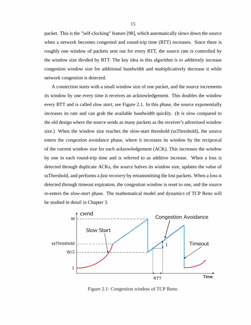
A connection starts with a small window size of one packet, and the source increments
its window by one every time it receives an acknowledgement. This doubles the window
every RTT and is calledslow start, see Figure 2.1. In this phase, the source exponentially
increases its rate and can grab the available bandwidth quickly. (It isslow compared to
the old design where the source sends as many packets as the receiver’s advertised window
size.) When the window size reaches the slow-start threshold (ssThreshold), the source
enters thecongestion avoidancephase, where it increases its window by the reciprocal
of the current window size for each acknowledgement (ACK). This increases the window
by one in each round-trip time and is referred to as additive increase. When a loss is
detected through duplicate ACKs, the source halves its window size, updates the value of
ssThreshold, and performs afast recoveryby retransmitting the lost packets. When a loss is
detected through timeout expiration, the congestion window is reset to one, and the source
re-enters theslow-startphase. The mathematical model and dynamics of TCP Reno will
be studied in detail in Chapter 3.
cwnd
TimeTime
Slow Start
W Congestion Avoidance
RTT
1
W/2
ssThreshold
1
Timeout
Figure 2.1: Congestion window of TCP Reno.

16
There are some drawbacks in using packet loss as an indication of congestion. First,
high utilization can be achieved only with full queues, i.e., when the network operates at the
boundary of congestion [98]. This is ill-suited to the heavy-tailed TCP traffic, as observed
in [162, 91, 167]. While most TCP connections are “mice” (small, requiring low latency
[53]), a few “elephants” (long TCP connections, tolerating large latency) generate most of
the traffic. First, operating around a state with full queue, the mice suffer unnecessary loss
and queuing delay. Second, the performance of a loss-based TCP source will be degraded
in the situation where losses are due to other effects (e.g., wireless links).
There are also some other TCP alternatives we will briefly describe below.
2.1.2 TCP Vegas
Instead of using packet loss as a measure of congestion, there is another class of congestion
control algorithms that adapt their congestion window size based on end-to-end delay. This
approach is originally described by Jain [65] and is represented by TCP Vegas [19, 20] and
FAST TCP [69].
There are several key differences between TCP Vegas and TCP Reno. In slow-start
phase, TCP Vegas incorporates its congestion detection mechanism into slow-start with
minor modifications to grow the window size more cautiously. When packet loss is de-
tected, TCP Vegas uses a new retransmission mechanism and treats the receipt of certain
ACKs as a trigger to check if a timeout should happen [19]. The most important difference
between them is that TCP Vegas updates its congestion window size based on end-to-end
delay.
TCP Vegas source estimates its round-trip propagation delay as the minimal RTT, mea-
suring the current RTT for each ACK received. Then, it can figure out the number of its
own packets buffered along the path as the product of end-to-end queueing delay and its
sending rate. The source will try to keep this number in a region, specified by two param-
etersα andβ. The window size linearly increases, decreases, or maintains the same by
comparing this number withα andβ. The aim is to maintain a small number of packets in
the buffer to fully utilize the link and experience a small queueing delay.

17
Low et al. [101] provided a duality model for TCP Vegas and studied its equilibrium in
detail. It is shown that TCP Vegas achieves weighted proportional fairness at the equilib-
rium when there is sufficient buffer. Choe and Low [24] studied the dynamics of the TCP
Vegas algorithm, showing that it can become unstable in the presence of network delay,
and provided modification for better stability.
2.1.3 FAST TCP
It is shown [100, 59] that the current congestion control algorithms, TCP Reno, and its
variants do not scale with bandwidth-delay products of the Internet as it continues to grow,
and will eventually become performance bottlenecks. This has motivated the design of
FAST TCP [69, 70], which targets high-speed networks with long latency. Unlike other
congestion control algorithms, it is designed based on a theoretical framework [98, 102]
and aims to achieve high throughput while maintaining a stable and fair equilibrium.
FAST TCP adjusts its congestion window size based on queueing delay instead of
packet loss. In networks with large bandwidth-delay products, packet losses are rare events,
and each packet loss only provides one bit of information. The queueing delay can be mea-
sured for each ACK packet, and the results provide multi-bit information. The measured
queueing delay is processed with a low-pass filter to provide more accurate and smooth
information about the congestion in the networks. This measured queueing delay is fed
into an equation to decide the changes in the congestion window size. In the congestion
avoidance phase, FAST periodically updates the congestion window according to [69]:
w ←− min
{2w, (1− γ)w + γ
(baseRTT
RTTw+ α
) }
whereγ ∈ (0, 1], baseRTT is the minimum RTT observed so far, andα is a constant.
Although FAST TCP and TCP Vegas have different window update algorithms and dy-
namics, they share the same equilibrium properties. Similar to TCP Vegas, FAST achieves
weighted proportional fairness, and the constantα is also the number of packets a flow
attempts to maintain in the network buffers at equilibrium.
There are some other important implementation features of FAST that are not described

18
here, for example, burst control and window pacing. The details of the architecture, algo-
rithms, extensive experimental evaluations of FAST TCP, and comparison with other TCP
variants can be found in [68]. I will provide mathematical models of FAST TCP, and will
study its dynamics in detail in Chapter 4.
There are also some other TCP congestion control proposals for high-speed networks,
which will not be covered in detail here. The eXplicit Congestion control Protocol (XCP)
[76], proposed by Katabi et al., is designed based on control theory and requires explicit
feedback from the routers to achieve stability and fairness. The High Speed TCP (HSTCP)
[39], proposed by Floyd, is a modification of current TCP to increase more aggressively and
decrease more cautiously in large congestion window situations. The scalable TCP [81],
proposed by Kelly, uses multiplicative increase and multiplicative decease instead of TCP
Reno’s AIMD. The BIC TCP [163], proposed by Xu et al., uses binary search increase and
additive increase. See [21, 118] for experiments and performance comparisons between
these new proposals.
2.2 Active Queue Management (AQM)
The AQM algorithm runs on a router, which updates and feedbacks congestion information
to end-users. The feedback is usually in the form of packet loss, delay, or marking. There
is a very large body of AQMs proposed, and I will just describe few common AQMs in this
subsection.
2.2.1 Droptail
Droptail is the simplest AQM scheme in the current Internet. It is just a first-in-first-
out(FIFO) queue with limited capacity, and it simply drops any incoming packets when
the queue is full. Since it is simple and easy to implement, Droptail is the dominant AQM
in the current Internet. This FIFO queue helps to achieve better link utilization and absorbs
the bursty traffic.
The congestion information in a Droptail queue is updated by the queueing process and

19
is represented by the size of the backlog buffer. The delay-based TCP algorithms, e.g.,
TCP Vegas and FAST, receive this information by sensing the changes in the round-trip
delay. The dynamics of FAST TCP will be studied in Chapter 4 using Droptail routers with
sufficient buffer.
For loss-based sources, the Droptail queue sends back one bit of information by a packet
drop, which indicates that the router buffer is full and the network is congested. When
working with TCP Reno, Droptail routers have two drawbacks: thelock-outand thefull-
queuephenomena, which are pointed out in Braden et al. [17]. Thelock–outphenomenon
involves a single or a few sources that monopolize the bandwidth. This situation is usually
the result of synchronization [55, 117]. Thefull-queuephenomenon refers to the effect
that the queue can be full (or almost full) for long periods of time, which produces large
end-to-end delays.
One possible solution to overcome these problems is to detect congestion early and to
convey congestion notification to sources before queue overflow. We describe one such
solution below.
2.2.2 Random Early Detection (RED)
The Random Early Detection algorithm, or RED, is proposed by Floyd and Jacobson [41] to
solve the synchronization and full queue problems of Droptail. In contrast to Droptail that
drops packets deterministically when the buffer is full, the RED algorithm drops arriving
packets probabilistically based on average queue size. The packet is dropped randomly to
break up synchronized processes that lead to the lock-out phenomenon, and RED controls
the average queue size to avoid queue overflow.
There are two components in the RED algorithm. The first is the estimation of average
queue size using the exponential weighted average, which can also be interpreted as a low
pass filter to get rid of noise. The other part of the algorithm decides whether to drop an
incoming packet. There are three RED parametersminth , maxth , andmaxp controlling
the dropping probability as shown in Figure 2.2. When the average queue size is less
than the minimum thresholdminth , the dropping probability is zero. When it exceeds

20
the maximum thresholdmaxth , all the incoming packets will be dropped. When it is in
between, packets will be dropped with a probability that varies linearly from 0 tomaxp.
maxth avg. queue size
p
minth
maxp
Figure 2.2: RED dropping function.
The RED can also mark the incoming packets instead of dropping them with the deploy-
ment of Explicit Congestion Notification (ECN) [131] to prevent packet loss and improve
throughput. The basic idea of ECN is to give the network the ability to explicitly signal
TCP sources of congestion using one additional bit in the IP packet header and to have the
TCP sources reduce their transmission rates in response to the marked packets.
The dynamics of Reno/RED systems will be studied in details in Chapter 3. It is shown
that the system becomes unstable when the delay increases or when the link capacity in-
creases. It is very difficult to configure the RED parameters to achieve better performance.
There has been a large body of AQM schemes proposed recently. Some notable exam-
ples include, Stabilized RED [123], PI controller [58], REM [5] , AVQ [86], BLUE [35],
etc.
2.2.3 CHOKe
CHOKe [126], which stands for “CHOose and Keep for responsive flows, CHOose and
Kill for unresponsive flows”, is proposed by Pan et al. in 2001. It aims to penalize the un-
responsive flows (e.g., UDP sources), to protect the rate-adaptive flows (e.g., TCP sources),
and to ensure fairness.
The scheme, CHOKe, is particularly interesting in that it does not require any state
information and yet can provide a minimum throughput to TCP flows. The basic idea of
21
CHOKe is explained in the following quote from [126]:
When a packet arrives at a congested router, CHOKe draws a packet at random from
the FIFO (first-in-first-out) buffer and compares it with the arriving packet. If they both
belong to the same flow, then they are both dropped; else the randomly chosen packet
is left intact and the arriving packet is admitted into the buffer with a probability that
depends on the level of congestion (this probability is computed exactly as in RED).
The surprising feature of this extremely simple scheme is that it can bind the bandwidth
share of UDP flows regardless of their arrival rate.
Its queue characteristics and the maximum throughput of unresponsive flows is studied
in [143, 155, 145]. These results will be briefly covered in Section 7.2.
2.3 Unified frameworks for TCP/AQM systems
In this subsection, we will review the general frameworks for studying the equilibrium and
dynamics of TCP/AQM systems. These models will be used throughout this dissertation.
2.3.1 General dynamic model of TCP/AQM
A network is modelled as a set ofL links with finite capacitiesc = (cl, l ∈ L). They are
shared by a set ofN sources indexed byi. Each sourcei uses a subsetLi ⊆ L of links.
The setsLi define anL×N routing matrix
Rli =
1 if l ∈ Li
0 otherwise. (2.1)
We use the deterministic flow model developed in [115, 99] to describe transmission
rates. Two assumptions are made when using this model. First, the packets are infinitely
small and the sending rate is differentiable (like fluid flow). Second, the congestion signal
is fed back continuously.

22
Each sourcei has an associated transmission ratexi(t), and each linkl has an aggregate
incoming flow rateyl(t). Since all sources whose paths include linkl contribute toyl(t),
we have the equation:
yl(t) =∑
i
Rlixi(t− τ fli), (2.2)
whereτ fli denotes the forward transmission delay from sourcei to link l.
Each link l has an associatedcongestion measure(or price) pl(t), which is a non-
negative quantity maintained by AQM algorithms. The sources are assumed to have access
to the aggregate price of all links in their route1,
qi(t) :=∑
l
Rlipl(t− τ bli), (2.3)
whereτ bli denotes the backward transmission delay from linkl to sourcei. The total round-
trip time τi for sourcei thus satisfies
τi = τ fli + τ b
li
for every linkl in its path.
As shown in [96], this model includes, to a good approximation, the mechanism present
in existing protocols with a different interpretation for price in different protocols (e.g.,
marking or dropping probability in TCP Reno, queueing delay in TCP Vegas).
In this framework, a complete feedback-control system is specified by supplying two
additional blocks: the source rates change according to aggregate prices in the TCP algo-
rithm and the link prices update based on link utilization. The complete system determines
both the equilibrium and dynamic characteristics of the TCP/AQM network.
Since the TCP/AQM is decentralized, the sources only have access to their local in-
formation. Therefore, the key restriction in the above control laws is that they must be
1This is true when delay is used as congestion price. It is approximately true for random marking anddropping when the probability is small.

23
decentralized. Therefore, we can model the dynamics of TCP in a general form
xi(t) = Fi(xi(t), qi(t)). (2.4)
Similarly, the dynamics at links can be written as2
pl(t) = Gl(pl(t), yl(t)). (2.5)
The overall structure of this congestion control system is shown in Figure 2.3.
F1
FN
F1
FN
G1
GL
G1
GL
∑ −=i
f
liilil txRty )()( τ∑ −=i
f
liilil txRty )()( τ
∑ −=l
b
lillii tpRtq )()( τ∑ −=l
b
lillii tpRtq )()( τ
y
pq
x
TCP AQM
Figure 2.3: General congestion control structure.
We will study the dynamics of TCP within this general framework in Chapter 3 and 4.
The equilibrium properties will be studied with the duality model introduced in the next
subsection.
2.3.2 Duality model of TCP
In this section, it will be shown that the above feedback-control system solves a utility
maximization problem at its equilibrium.
Suppose that the equilibrium rates and prices are given byx∗, y∗, p∗, andq∗. Based on
2A more accurate formulation is given in [96] that includes the internal variables of AQM in the parametersof Gl.

24
(2.3) and (2.2), we have following equilibrium relationships
y∗ = Rx∗, q∗ = RT p∗. (2.6)
Assume that equilibrium rates satisfy
x∗i = fi(q∗i ), (2.7)
wherefi(·) is implicitly defined byFi(x∗, q∗i ) = 0 or given by the source static law, e.g.,
[97]. fi(·) is usually a positive, strictly monotonic decreasing function, since the source
decreases its rate with increasing congestion.
Let f−1i (xi) be the inverse function of (2.7), and let a utility functionUi(xi) be its
integral
Ui(xi) :=
∫f−1
i (xi)dxi. (2.8)
This relation implies thatUi(xi) is a monotonic increasing and strictly concave function. It
is easy to check that the equilibrium ratex∗i uniquely solves
maxxi≥0
Ui(xi)− xiq∗i . (2.9)
We interpretUi(xi) as the benefit the source receives by transmitting at ratexi andq∗i as the
price per unit. Then (2.9) is a maximization of the source’s profit. This interpretation makes
few assumptions regarding TCP and AQM and can be used for various TCP schemes.
The global optimization problem to maximize aggregate utility with capacity con-
straints is formulated by Kelly in [77, 80],
maxx≥0
∑i
Ui(xi) (2.10)
subject to Rx ≤ c. (2.11)
It has a unique solution, since it is maximizing a concave function over a convex set. Now

25
we interpret the equilibrium price as the dual variables (or as the Lagrange multipliers) for
the problem (2.10-2.11). Then its Lagrangian is
L(x, p) =∑
i
Ui(xi)−∑
l
pl(yl − c) =∑
i
(Ui(xi)− qixi) +∑
l
plcl. (2.12)
The dual problem is
minp≥0
∑i
Bi(qi) +∑
l
plcl, (2.13)
where
Bi(qi) = maxxi≥0
Ui(xi)− xiqi. (2.14)
Convex duality implies that at the optimump∗, the correspondingx∗, which maximizes
individual optimality (2.9), is exactly the unique solution to the primal problem (2.10-2.11)
since (2.14) is identical to (2.9). Therefore, provided the equilibrium pricesp∗ can be made
to align with the Lagrange multipliers, the equilibrium ratex∗ solves the primal problem in
a distributed way. It is proven in [96] that any link algorithm that satisfies
y∗l ≤ cl with equality ifp∗ > 0 for anyl (2.15)
will guarantee this alignment. In this case,x∗ is the unique primal optimal solution, and
p∗ is a dual optimal solution. It has been argued [96] that the condition (2.15) is satisfied
by any AQM that stabilizes the queue, e.g., RED, REM, and Droptail. Therefore, various
TCP/AQM protocols can be interpreted as different distributed primal-dual algorithms to
solve the global optimization problem (2.10-2.11) with different utility functions.
The equilibrium structures of different congestion control schemes are characterized by
their corresponding utility functions. This model provides us with a rigorous framework
in which to study various equilibrium properties such as fairness, efficiency, and effects of
different network parameters. In Chapter 6, I will present the methods and results following
this approach.

26
This optimization framework can also be extended to study the interaction of TCP at a
fast timescale and IP routing at a slow timescale. See Chapter 5 for details.

27
Chapter 3
Local Dynamics of Reno/RED
3.1 Introduction
It is well known that TCP Reno/RED can oscillate wildly and it is extremely hard to reduce
the oscillation by tuning RED parameters, e.g., [110, 25]. This oscillation could be the
outcome of the AIMD bandwidth probing strategy employed by TCP Reno and noise-like
traffic that are not effectively controlled by TCP (e.g., short lived TCP source). Recent
models e.g., [36, 59], imply however that oscillation is an inevitable outcome of the pro-
tocol itself. We present more evidence to support this view. We argue that Reno/RED
oscillates not only because of the AIMD probing and noise traffic, but more fundamentally,
it is due to instability. Therefore, even if there is no AIMD, and the congestion window is
periodically adjusted by the average of AIMD based on loss probability, the oscillation per-
sists. We illustrate usingns-2simulations that, after smoothing out the AIMD component
of the oscillation, the average behavior can either be steady with small random fluctuations
(when the protocol is stable), or exhibit limit cycles of amplitude much larger than ran-
dom fluctuations (when it is unstable). Moreover, this qualitative behavior persists even
when a large amount of noise traffic is introduced, and even when sources have different
delays. We conclude that it is the protocol stability that largely determines the dynamics of
Reno/RED.
This motivates the stability characterization of Reno/RED. In Section 3.3 we develop a
general nonlinear model of Reno/RED. The equilibrium structure of this system is analyzed
using duality model, and a unique equilibrium exists because it is the unique solving of the

28
underling utility maximization problem, see [96] for details. Here, we study local stability
by linearizing the model around this equilibrium. The linear model generalizes the single
link identical source model of [59]. We validate our model with simulations and illustrate
the stability region of Reno/RED. We derive a sufficient stability condition for the special
case of a single link withheterogeneoussources. It shows that Reno/RED becomes unstable
when delay increases, or more strikingly, when link capacity increases!
In the linearized model, the gain introduced by TCP Reno increases rapidly with delay
and link capacity. This induces instability and makes compensation by RED extremely
difficult. In particular, RED parameters can be tuned to improve stability, but only at the
cost of a large queue, even when they are dynamically adjusted. Our results suggest that
Reno/RED is ill suited for future high-speed networks, which motivates the design of new
distributed algorithms for high speed long latency networks.
3.2 Motivation
Why does Reno/RED oscillate? What is the effect of AIMD probing, noise traffic, and
heterogeneity of delays on average congestion window and instantaneous queue size? In
this section, we show that their effect is insignificant in comparison with that of protocol
instability. This protocol instability is the dominant reason for oscillation in the Reno/RED
system. Therefore, it is very important to study the protocol stability of Reno/RED system.
We simulate a single bottleneck network usingns-2. The bottleneck link has a capacity
9 pkts/ms with a constant packet size of 1000 bytes. The AQM running on this link is RED
with ECN marking inbytemode (i.e., ACK packets are marked with negligible probability).
The RED parameters aremaxp = 0.1,minth = 50 pkts,maxth = 550 pkts, and weight
for queues averagingα = 10−4. The link is shared by 50 persistent TCP Reno sources.
We have run simulations with both one-way and two-way traffic, and the behavior is very
similar. The results in Figures 3.1 and 3.2 are for two-way traffic, and those in Figure 3.3
are for one-way traffic. The measurements on the Internet [2] show that most connections
have round-trip delays between 15-500ms. We perform simulations within this range of
delays.

29
0 5 10 15 20 25 30 35 400
10
20
30
40
50
60
70
Win
dow
(pkt
s)
Individual windowAverage window
time(s)
Individual window
Average window
(a) Window (delay = 40ms)
0 5 10 15 20 25 30 35 400
100
200
300
400
500
600
700
800
Inst
aneous
queue(p
kts)
time(s)
(b) Queue (delay = 40ms)
0 5 10 15 20 25 30 35 400
20
40
60
80
100
120
140
Win
dow
(pkt
s)
Individual windowAverage window
time(s)
Individual window
Average window
(c) Window (delay = 200ms)
0 5 10 15 20 25 30 35 400
100
200
300
400
500
600
700
800
Inst
aneous
queue(p
kts)
time(s)
(d) Queue (delay = 200ms)
Figure 3.1: Window and queue traces without noise traffic.
Figure 3.1 gives the result of two cases where connections have identical roundtrip
propagation delay and generate traffic in both directions. Figure 3.1(a) shows an individual
window and the average window that is mean window size of all 50 sources, as a function
of time. They are typical traces when round-trip propagation delay is small (40ms in this
case). Oscillations due to AIMD are prominent in the individual window, but disappear
in the average window. Since the queue averages individual windows, it also displays a
smooth trace with small random fluctuations, as shown in Figure 3.1(b). We consider the
averagebehavior of the protocol stable (non-oscillatory) in this case.

30
Figures 3.1(c) and (d) show the corresponding windows and queue when round-trip
propagation delay is increased to 200ms. Not only does the individual window oscillate
with a larger amplitude, more importantly, its average displays a deterministic limit cycle.
This also shows up in the queue trace. We say the protocol is in anunstableregime.
What is the effect of noise-like mice traffics that are not effectively controlled by
Reno/RED? To get a qualitative understanding, we add additional short HTTP sources to
the 50 persistent bi-directional TCP flows. Each HTTP source sends a single-packet request
to its destination, which then replies with a file of size that is exponentially distributed. Af-
ter the source completely receives the data, it waits for a random time that is exponentially
distributed with a mean of 500 milliseconds and repeats the process. Both the request and
the response are carried over TCP connections. Two sets of simulations are conducted:
the first with 60 http sources generating 10% noise (i.e., persistent TCP sources occupied
90% of bottleneck link capacity), and the second set with 180 http sources generating 30%
noise.
The queue traces when propagation delays are 40ms (stable) and 200ms (unstable),
respectively, are shown in Figures 3.2(a) and (b) for a noise intensity of 10% and in Figure
3.2(c) and (d) for a noise intensity of 30%. The behavior of the queue is dominated by the
stability of the protocol, not by noise-like mice traffic (compare with Figures 3.1(b) and
(d)). In the stable regime (40ms delay), the noise traffic increases the average queue length
slightly. This increases the marking probability and reduces the average window of the
persistent TCP sources.
All our previous simulations are for sources with identical propagation delay. Will the
dynamic behavior be very different when sources have different delays? We repeat the
previous experiments, without noise, with 50 persistent connections having delays ranging
from 40ms to 64ms at 1ms increments, with 2 sources to each delay value. We study their
dynamic behavior when all delays are scaled up, or down, over a wide range. The behavior
is qualitatively similar to the case of identical delay, with more severe queue oscillation.
Figure 3.3(a) shows the instantaneous queue when the scaling factor is0.3 (delays range
from 12ms to19.2ms), with an average delay of15.6ms, averaged over all sources. Figure
3.3(b) shows the queue when the scaling factor is 4, with an average delay of 208ms.

31
0 5 10 15 20 25 30 35 400
100
200
300
400
500
600
700
800
Inst
aneous
queue(p
kts)
time(s)
(a) Queue (delay = 40ms, 10% noise)
0 5 10 15 20 25 30 35 400
100
200
300
400
500
600
700
800
Inst
ane
ou
s queue(p
kts)
time(s)
(b) Queue (delay = 200ms, 10% noise)
0 5 10 15 20 25 30 35 400
100
200
300
400
500
600
700
800
Inst
aneous
queue(p
kts)
time(s)
(c) Queue (delay = 40ms, 30% noise)
0 5 10 15 20 25 30 35 400
100
200
300
400
500
600
700
800
Inst
aneous
queue(p
kts)
time(s)
(d) Queue (delay = 200ms, 30% noise)
Figure 3.2: Queue traces with noise traffic.
Hence it is protocol stability that largely determines the dynamics of Reno/RED. We
now characterize when Reno/RED is stable.
3.3 Dynamic model
In this section we develop a model of Reno/RED and use it to study the local dynamics
of Reno/RED. We start with a nonlinear model, make a few remarks about its equilibrium
properties, and then linearize the model around the equilibrium. We validate our linear

32
0 10 20 30 40 50 60 70 80 90 1000
100
200
300
400
500
600
700
800
time (sec)
Instantaneous queue (pkts)
inst
anta
neou
s qu
eue
(pkt
s)
(a) Queue (delays from 12ms to 19ms)
0 10 20 30 40 50 60 70 80 90 1000
100
200
300
400
500
600
700
800
time (sec)
Instantaneous queue (pkts)
inst
anta
neou
s qu
eue
(pkt
s)
(b) Queue (delays from 160ms to 254ms)
Figure 3.3: Queue traces with heterogeneous delays.
model withns-2simulations and illustrate the stability region of Reno/RED. Finally we
derive a stability condition for the special case of a single link with heterogeneous sources.
3.3.1 Nonlinear model of Reno/RED
The general nonlinear model for TCP/AQM systems has been presented in Section 2.3.
Here more details are given in order to study Reno/RED systems.
A network is modelled as a set ofL links with finite capacitiesc = (cl, l ∈ L). They
are shared by a set ofN sources. The interactions between them are specified by a routing
matrixR whereRli = 1 if link l is in the path of sourcei, andRli = 0 otherwise.
Denoteτi(t) as the round-trip time of sourcei at time t; it is the sum of round-trip
propagation delaydi and the round-trip queueing delay∑
l Rlibl(t)/cl. Sourcei’s sending
ratexi(t) can be formulated as
xi(t) =wi(t)
τi(t), (3.1)
wherewi(t) denotes the congestion window size. The aggregate flow rate at linkl is
yl(t) =∑
i
Rlixi(t− τ fli(t)), (3.2)

33
whereτ fli(t) is the forward delay from sourcei to link l.
The link congestion pricepl(t) in the general model corresponds to the packet marking
(or loss) probability in TCP Reno. The end-to-end marking probability observed at sourcei
is actuallyqi(t) = 1−∏l∈Li
(1−pl(t−τ bli(t))) whereτ b
li(t) is the backward delay from link
l to sourcei. We assume thatpl(t) is small for allt so that, approximately, the end-to-end
probability is
qi(t) =∑
l
Rlipl(t− τ bli(t)). (3.3)
The forward and backward delays are related to the round-trip time through
τi(t) = τ fli(t) + τ b
li(t)
for all l ∈ Li.
We now model TCP Reno and RED to provide the(F, G) functions in the general
framework. We focus on the AIMD algorithm of TCP Reno at thecongestion avoidance
phase. The congestion window change in this phase has been described in Section 2.1. At
time t, sourcei transmits at ratexi(t) packets/second; hence, it receives acknowledgments
at ratexi(t− τi(t)), assuming every packet is acknowledged. A fraction(1−qi(t)) of these
acknowledgments are positive, each incrementing the windowwi(t) by 1/wi(t); hence the
windowwi(t) increases, on average, at the rate ofxi(t− τi(t))(1− qi(t))/wi(t). Similarly
negative acknowledgments are received at an average rate ofxi(t−τi(t))qi(t), each halving
the window, and hence the windowwi(t) decreases at a rate ofxi(t − τi(t))qi(t)wi(t)/2.
Hence, the window evolves under Reno according to
wi(t) = xi(t− τi(t))(1− qi(t))1
wi(t)− xi(t− τi(t))qi(t)
wi(t)
2, (3.4)
whereqi(t) is given by (3.3).
To model RED, letbl(t) denote the instantaneous queue length at timet that evolves
34
according to
bl(t) = yl(t)− cl, (3.5)
whereyl(t) is the flow rate given by (3.2) andcl is the link capacity. Define the average
queue length asrl(t). It is updated according to
rl(t) = −αlcl (rl(t)− bl(t)), (3.6)
whereα is the averaging weight. Given the average queue lengthrl(t), the marking proba-
bility is given by
pl(t) =
0 rl(t) ≤ bl
ρl(rl(t)− bl) bl < rl(t) < bl
1 rl(t) ≥ bl
, (3.7)
wherebl, bl, andpl are RED parameters, andρl = pl/(bl − bl).
In summary, Reno/RED is modelled by (3.4–3.7), and their interconnection through the
network is modelled by (3.2–3.3).
The equilibrium of this system is studied in [96, 101]. The Reno/RED model is inter-
preted as carrying out a distributed, primal-dual algorithm to maximize the aggregate utility
over the Internet. The utility function of TCP Reno is derived to be
Ui(xi) =
√2
τi
tan−1
(τixi√
2
).
The equilibrium properties can be studied by solving the underlying convex program. It
also implies that the Reno/RED system has a unique equilibrium.
3.3.2 Linear model of Reno/RED
We linearize the Reno/RED equations (3.4-3.7) to study its stability around equilibrium.
We make several simplifying assumptions. First we assume that the routing matrixR has

35
full row rank so there is a unique equilibrium loss probability vectorp. Second, only
congested links at the equilibrium are considered in the linear model. Moreover we assume
that the system operates in regionbl < rl(t) < bl, so that the marking probability is affine
in the average queue length,pl(t) = ρl(rl(t)− bl).
We make a key assumption on the time-varying, round-trip delay. Round-trip delay ap-
pears in two places: first, in the relation between windowwi(t) and ratexi(t), as expressed
in (3.1), and second, in the time argument of flow rateyl(t), as expressed in (3.2), and
the end-to-end marking probabilityqi(t), as expressed in (3.3). Inclusion of instantaneous
queueing delay in the first place yields a qualitatively different model than if queueing de-
lay is ignored or assumed constant. It means that the queue is not an integrator but has more
complicated dynamics; see (3.9) below. As the proof of Theorem 3.1 shows, this dynamic
is critical to the stability of Reno/RED. The resulting linear model matches simulations
significantly better than if queueing delay is assumed constant. Time-varying delay in the
second place makes linearization difficult, and we replace it by its (constant) equilibrium
value (including equilibrium queueing delay). We approximate the delaysτi(t), τ fli(t), and
τ bli(t) by their equilibrium values in (3.2) and (3.3). With these assumptions, we linearize
Reno/RED around the unique equilibrium. From (3.4), Reno becomes
wi(t) =
(1−
∑
l
Rlipl(t− τ bli)
)wi(t− τi)
τi(t− τi)
1
wi(t)− 1
2
∑
l
Rlipl(t− τ bli)
wi(t− τi) wi(t)
τi(t− τi).
Let w∗i , p
∗l , . . . be equilibrium quantities andδwi(t) = wi(t)− w∗
i , . . . . be the small varia-
tions near the equilibrium. Linearization yields
δwi(t) = − 1
τiq∗i
∑
l
Rliδpl(t− τ bli) −
q∗i w∗i
τi
δwi(t).
Around the equilibrium, the buffer process under RED evolves according to
bl(t) =∑
l
Rliwi(t− τ f
li)
τi(t− τ fli)
− cl =∑
l
Rliwi(t− τ f
li)
di +∑
k Rkibk(t− τ fli)/ck
− cl.
Let τi = di +∑
k Rkib∗k/ck be the equilibrium round-trip time (including queueing delay).
36
Linearizing, we have
δbl(t) =∑
i
Rliδwi(t− τ f
li)
τi
−∑
k
∑i
RliRki δbk(t− τ fli)
w∗i
τ 2i ck
.
The second term above is ignored if we have neglected or assumed constant the queueing
delay in round-trip time. The double summation sums over all linksk that share any source
i with link l. It says that the link dynamics in the network are coupled through shared
sources. The termδbk(t − τ fli)w
∗i /(τick) is roughly the backlog at linkk due to packets of
sourcei, under FIFO queueing. Hence the backlogbl(t) at link l decreases at a rate that
is proportional to the backlog of this shared sourcei at another linkk. This is because
backlog in the path of sourcei reduces therate at which sourcei packets arrive at linkl,
decreasingbl(t).
Putting everything together, Reno/RED is described by, in Laplace domain,
δw(s) = −(sI + D1)−1D2R
Tb (s)δp(s),
δp(s) = (sI + D3)−1D4δb(s),
δb(s) = (sI + Rf (s)D5RT D6)
−1Rf (s)D7δw(s),
where the diagonal matrices areD1 = diag (q∗i w∗i /τi), D2 = diag (1/(τiq
∗i )), D3 =
diag (αlcl), D4 = diag (αlclρl), D5 = diag (w∗i /τ
2i ), D6 = diag (1/cl), andD7 =
diag (1/τi), andRf (s) and Rb(s) are delayed forward and backward routing matrices,
defined as
[Rf (s)]li =
e−τflis if l ∈ Li
0 otherwise, and [Rb(s)]li =
e−τblis if l ∈ Li
0 otherwise..(3.8)
This model generalizes the single-link, identical-source model of [59] to multiple links
with heterogeneous sources.

37
3.3.3 Validation and stability region
We present a series of experiments to validate our linear model when the system is stable
or barely unstable, and to illustrate numerically the stability region.
We consider a single link of capacityc pkts/ms shared byN sources with identi-
cal round-trip propagation delayd ms. ForN = 20, 30, . . . , 60 sources, capacityc =
8, 9, . . . , 15 pkts/ms, and propagation delayd = 50, 55, . . . , 100 ms, we examine the
Nyquist plot of the loop gain of the feedback system (L(jω) in (3.9) below). For each
(N, c) pair, we determine the delaydm(N, c), at5ms increments, at which the smallest in-
tercept of the Nyquist plot with the real axis is closest to−1. This is the delay at which the
system(N, c) transits from stability to instability according to the linear model. For this
delay, we compute the critical frequencyfm(N, c) at which the phase ofL(jω) is−π. Note
that the computation ofL(jω) requires equilibrium round-trip timeτ , the sum of propa-
gation delaydm(N, c), and equilibrium queueing delay. The queueing delay is calculated
from the duality model [96]. Hence, for each(N, c) pair that becomes barely unstable at
a delay between 50ms and 100ms, we obtain the critical (propagation) delaydm(N, c) and
the critical frequencyfm(N, c) from the analytical model. For all experiments, we have
fixed the parameters atα = 10−4, ρ = 0.1/(540− 40) = 0.0002.
We repeat these experiments inns-2, using persistent TCP sources and RED with ECN
marking. The RED parameters are (0.1, 40pkts, 540pkts,10−4), corresponding to theα and
ρ values in the model. For each(N, c) pair, we examine the queue and window trajectories
to determine the critical delaydns(N, c) when the system transits from stability to insta-
bility. We measure the critical frequencyfns(N, c), the fundamental frequency of queue
oscillation, from the fast fourier transform of the queue trajectory. Thus, corresponding
to the linear model, we obtain the critical delaydns(N, c) and frequencyfns(N, c) from
simulations.
We compare model prediction with simulation. Figure 3.4(a) plots the critical delay
dns(N, c) from ns-2simulations versus the critical delaydm(N, c) computed from the lin-
ear model. Each data point corresponds to a particular(N, c) pair. The dashed line is where
all points should lie if the linear model agrees perfectly with the simulation. Figure 3.4(b)

38
50 55 60 65 70 75 80 85 90 95 10050
55
60
65
70
75
80
85
90
95
100Round trip propagation delay at critical frequency (ms)
delay (NS)
de
lay (
mo
de
l)
30 data points
(a) Critical delay (ms)
0 0.5 1 1.5 2 2.5 3 3.5 4 4.5 50
0.5
1
1.5
2
2.5
3
3.5
4
4.5
5Critical frequency (Hz)
frequency (NS)
fre
qu
en
cy (
mo
de
l)
dynamiclink model
staticlink model
30 data points
(b) Critical frequency (Hz)
Figure 3.4: Linear model validation.
gives the corresponding plot for critical frequenciesfns(N, c) versusfm(N, c). The agree-
ment between model and simulation seems quite reasonable (recall that delay values have
a resolution of 5ms).
Consider a static link model where marking probability is a function of link flow rate
pl(t) = fl(yl(t)).
Then the linearized model is
δpl(t) = f ′l (y∗l ) δyl(t),
wheref ′l (y∗l ) is the derivative offl evaluated at equilibrium. Also shown in Figure 3.4(b)
are critical frequencies predicted from this static-link model (withf ′l (y∗l ) = ρ = 0.0002;
this does not affect the critical frequency), using the same Nyquist plot method described
above. It shows that queue dynamics are significant at the time-scale of interest.
Figure 3.5 illustrates the stability region implied by the linear model. For eachN ,
it plots the critical delaydm(N, c) versus capacityc. The curve separates stable (below)
from unstable regions (above). The negative slope shows that Reno/RED becomes unstable

39
8 9 10 11 12 13 14 1550
55
60
65
70
75
80
85
90
95
100Round trip propagation delay at critical frequency
capacity (pkts/ms)
de
lay (
ms)
N=40
N=30
N=20
N=50 N=60
Figure 3.5: Stability region.
when delay or capacity is large. AsN increases, the stability region expands, i.e., small
load induces instability. Intuitively, a larger delay or capacity, or a smaller load, leads to
a larger equilibrium window; this confirms the folklore that TCP behaves poorly at large
window size.
3.4 Local stability analysis
We now characterize the stability region in the case of a single link withN heterogeneous
sources. Writing forward delay as a fractionβi ∈ (0, 1) of round-trip time,τ fi = βiτi, and
dropping link subscriptl, the open-loop transfer function is
L(s) = Rf (s)D7(sI + D1)−1D2R
Tb (s)(sI + D3)
−1D4(sI + Rf (s)D5RT D6)
−1
=∑
i
1
τip∗(τis + p∗w∗i )· αcρ
s + αc· 1
s + 1c
∑n
x∗nτn
e−βiτns· e−τis. (3.9)
The first term on the right-hand side describes Reno dynamics, the second term describes
RED averaging, the third term is the buffer process, and the last term represents network
delay. The special case where all sources have identical round-trip times,τi = τ , and
forward delays are zero,βi = 0, is analyzed in [59]. They provide sufficient conditions for
closed-loop stability and use them to tune RED parametersα andρ.

40
We start with a lemma that collects some equilibrium properties. It can be proved di-
rectly from the fixed point of (3.4)–(3.7). Letτ := maxi τi, τ := mini τi, τ := (∑
i 1/τi)−1,
andβ := maxi βi.
Lemma 3.1.Letp∗ be the equilibrium loss probability, and letw∗i andx∗i be the equilibrium
window and rate respectively. Thenp∗ = 2/(2 + (cτ)2), w∗i = cτ for all sourcesi, x∗i =
w∗i /τi and
∑i x
∗i /c = 1.
A sufficient condition for local stability is provided by the following theorem.
Theorem 3.1.The closed-loop system described by (3.9) is stable if
ρτ 2
τ τp∗2w∗1
(1 +
1
cτα+
1
p∗w∗1
)<
π(1− β)2
√4β
2+ π2(1− β)2
.
Proof. See [100] for detailed proof.
The left-hand side of the (sufficient) stability condition depends on network parameters
(c and τi) as well as RED parameters (α and ρ). The right-hand side is a property of
the network node that is independent of these parameters. For stability, the left-hand side
must be small. This requires small capacityc and delaysτi and largeN , confirming the
simulation results of the last section. To understand this, note thatcτ is the equilibrium
window size of all sources. Assumingw∗1 = cτ À 2 so thatp = 2/w∗2
1 , then the stability
condition can be re-written as
ρw∗3
1 N
4
(w∗
1
2+ 1 +
N
w∗1α
)<
π(1− β)2
√4β
2+ π2(1− β)2
.
This suggests that the system becomes unstable when window sizew∗1 becomes large,
agreeing with our empirical experience that TCP behaves poorly at large window size.
Roughly, whenc doubles, the equilibrium rate doubles, and hence the window is halved
with twice the magnitude at twice the frequency, resulting in a quadratic increase in control
gain and pushing the system into instability.
The dependence of the stability condition onc, τ , andN is most clearly exhibited in
the case of identical sources, withτ = τi = τ = τ = Nτ .

41
Corollary 3.1. Supposep = 2/w∗21 . Then the stability condition in Theorem 3.1 becomes
ρc3τ 3
4N2
(cτ
2N+ 1 +
1
αcτ
)<
π(1− β)2
√4β
2+ π2(1− β)2
.
The stability condition also suggests that a smallerρ and a largerα enhance stability.
A smallerρ implies a larger equilibrium queue length [96]. A largerα incorporates the
current queue length into the marking probability more quickly. See [100] for proofs of
this Corollary.
3.5 RED parameter setting
It is suggested in [34] that the RED parametermaxp be dynamically adjusted: reduce
maxp asN decreases and raise it otherwise. Raisingmaxp, or reducingmaxth-minth ,
is equivalent to increasingρ ( = maxp/(maxth-minth) ) in the direction consistent
with the stability condition in Theorem 3.1. Theorem 3.1 sets an upper bound onρ,
given N, c, andτ , and hence a lower bound on equilibrium queue length, to ensure sta-
bility. Adapting RED parameterscannotprevent the inevitable choice between stability
and performance: eitherρ is set small to stabilize the queue, around a large value, or,
alternatively, it is set large to reduce the queue, at the risk of violent oscillation. What
adaptation can hope to achieve is to dynamically find a good compromise when network
condition changes.
The same stability analysis can also be applied to other AQM schemes, such as Virtual
Queue [50, 85, 87] and REM/PI [5, 59], and clarifies the role of AQM. The stability proof
relies on bounding a set of the formK · co{h(v, θ)} to the right of(−1, 0). The gainK
and the trajectoryh depend on TCP as well as AQM. For instance, for the case of a single
link with capacityc shared byN identical sources with delayτ , TCP and network delay
contribute a factor
htcp =e−jv
jv + p∗w∗1

42
to the trajectoryh and a factor
Ktcp =c2τ 2
2N(3.10)
to the gainK, assuming the equilibrium window is large so thatp∗ = 2/w2i = 2N/cτ .
AQM compensates for the high gain introduced by TCP by shapingh and reducingK.
With RED, for instance,
h(v, θ) =1
jv + αcτ
e−jθ
v· htcp, and K =
cταρ
1− β·Ktcp.
The first term inh is due to RED averaging, the second term is due to queue dynamics that
also boundsθ ≤ θ0. Hence both the queue and RED add phase lag toh. More importantly,
RED adds anothercτ to the gainK, necessitating a smallαρ for stability and leading to
sluggish response and large equilibrium queue. The factorτ/(1− β) in K comes from the
queue.
The high gainKtcp in (3.10) is mainly responsible for instability at high delay, high
capacity or low load. It makes it difficult for any AQM algorithm to stabilize the current
TCP.
3.6 Conclusion
We have presented simulation results to demonstrate that it is protocol stability more than
other factors that determine the dynamics of TCP/RED. We have developed a multi-link,
multi-source model that can be used to study the stability of general TCP/AQM. We have
presented a sufficient stability condition for the case of a single link with heterogeneous
sources and illustrated the form of Reno/RED’s stability region. It implies that Reno/RED
becomes unstable when the network scales up in delay or capacity. Our analysis indicates
the role, and the difficulty, of RED in stabilizing Reno.

43
Chapter 4
Modelling and Dynamics of FAST
4.1 Introduction
Congestion control is a distributed feedback algorithm to allocate network resources among
competing users. The algorithms in the current Internet, TCP Reno and its variants, have
prevented severe congestion while the Internet underwent explosive growth during the last
decade. In the previous chapter, we have shown that TCP Reno is ill suited for the future
high-speed networks. It is well known that it does not scale as the bandwidth-delay product
as the Internet continues to grow [59, 100]. This has motivated several recent proposals for
congestion control of high-speed networks, including HSTCP [39], Scalable TCP [81],
FAST TCP [69], and BIC TCP [163] (see [69] for extensive references). We have briefly
described the motivation, background theory, and congestion window update functions of
FAST TCP in Chapter 2. The details of the architecture, algorithms, extensive experimental
evaluations of FAST TCP, and comparison with other TCP variants can be found in [69].
Local stability of FAST TCP in the absence of feedback delay is proved in [69] for the case
of a single link. We extend the analysis to local stability with feedback delay and global
stability without feedback delay, both for general networks.
Most of the stability analysis in the literature is based on the fluid model introduced in
[59] (see surveys in [98, 79, 138] for extensions and related models). Key features of many
of these models are that a source controls its sending rate directly1 and that the queueing
1Even when the congestion window size is used as the control variable, sending rate is often taken to bethe window normalized by aconstantround-trip time, and hence a source still controls its rate directly.

44
delay at a link is proportional to the integral of the excess demand for its bandwidth.
In reality, a source dynamically sets its congestion window rather than its sending rate.
These models do not adequately capture the self-clocking effect where a packet is sent only
when an old one is acknowledged, except briefly and immediately after the congestion win-
dow is changed. This automatically constrains the inputrate at a link to the link capacity,
after a brief transient, no matter how large the congestion windows are set. Recently, a
new discrete-time link model was proposed in [160, 69] to capture this effect, and detailed
experimental validations have been carried out in [160]. While the traditional continuous-
time link model does not consider self-clocking, the new discrete-time link model ignores
the fast dynamics at the links. We first present both models of FAST TCP in Section 4.2.
Experimental results are provided to show that, despite errors in these models, both of them
track queueing delays reasonably well.
In Section 4.3, we prove that FAST TCP is globally stable for arbitrary networks when
there is no feedback delay using the continuous-time model. We also derive a sufficient
condition for local asymptotic stability for arbitrary networks with feedback delay, using
the techniques developed in [125, 152]. This condition is also necessary when the sources
are homogeneous with a single bottleneck link. We compare the predictions of stability
based on this condition to experiments on the Dummynet Testbed with such topology. Our
experiments suggest that FAST TCP is always stable for homogeneous sources with a sin-
gle link, while the model with delay predicts instability when the delay is large. We conjec-
ture that this conflict maybe due to the self-clocking effect ignored in the continuous-time
model.
In Sections 4.4, we analyze the stability of FAST TCP using the discrete-time model.
First, we prove that local asymptotic stability of FAST TCP in arbitrary networks in the
presence of delay depends on feedback delays only through their heterogeneity. It implies
in particular that a network where all sources have the same delay is always stable, no
matter how large the delay is. It also confirms the common belief that a slower update
enhances stability. Then we restrict ourselves to a single link without feedback delay and
prove the global stability of FAST TCP. The techniques developed for this discrete-time
model are new and applicable to analyzing other protocols.

45
Finally, we conclude in Section 4.5 with limitations of this work.
4.2 Model
4.2.1 Notation
A network consists of a set ofL links indexed byl with finite capacitycl. It is shared by a
set ofN flows identified by their sources indexed byi. Let R be the routing matrix where
Rli = 1 if sourcei uses linkl, and0 otherwise.
We uset for time in the continuous model, and for time step in the discrete-time model.
The meaning oft should be clear from the context. FAST TCP updates its congestion
window every fixed time period, which is used as the time unit.
Let di denote the round-trip propagation delay of sourcei, andqi(t) denote the round-
trip queueing delay. The round-trip time is given byTi(t) := di + qi(t). We denote the
forward feedback delay from sourcei to link l by τ fli and the backward feedback delay
from link l to sourcei asτ bli. The sum of forward delay from sourcei to any link l and
the backward delay from linkl to sourcei is fixed, i.e.,τi := τ fli + τ b
li for any link l on
the path of sourcei. We make a subtle assumption here. In reality, the feedback delays
τ fli , τ b
li include queueing delay and are time-varying. We assume for simplicity that they
are constant, and mathematically unrelated toTi(t). Later, when we analyze linear stability
around the network equilibrium in the presence of feedback delay, we can interpretτi as
the equilibrium value ofTi.
Let wi(t) be sourcei’s congestion window at timet (discrete or continuous time). The
sending rate of sourcei at timet is defined as
xi(t) =wi(t)
Ti(t), (4.1)
whereTi(t) = di + qi(t). The aggregate rate at linkl is
yl(t) =∑
i
Rlixi(t− τ fli). (4.2)

46
Let pl(t) be the queueing delay at linkl. The end-to-end queueing delayqi(t) observed by
sourcei is
qi(t) =∑
l
Rlipl(t− τ bli). (4.3)
4.2.2 Discrete and continuous-time models
FAST TCP source periodically updates its congestion windoww based on the average RTT
and estimated queueing delay. The pseudo-code is
w← (1− γ)w + γ
(baseRTT
RTTw+ α
),
whereγ ∈ (0, 1], baseRTT is the minimum RTT observed, andα is a constant. We model
this by the following discrete time equation
wi(t + 1) = γ
(diwi(t)
di + qi(t)+ αi
)+ (1− γ)wi(t), (4.4)
wherewi(t) is the congestion window of theith source,γ ∈ (0, 1], andαi is a constant for
sourcei. The corresponding continuous-time model is
wi(t) = γ
(diwi(t)
di + qi(t)+ αi − wi(t)
), (4.5)
where the time is measured in the unit of update period in FAST TCP.
For the continuous-time model, queueing delay has been traditionally modelled with
pl(t) =1
cl
(yl(t)− cl). (4.6)
However, TCP uses self-clocking: the source always tries to maintain that the number
of packets in fly equals to the congestion window size. When the congestion window is
fixed, the source will send a new packet exactly after it receives an ACK packet. When the
congestion window changes, the source sends out bulk traffic in burst, or sends nothing in
a short time period. Therefore, one round-trip time after a congestion window is changed,
packet transmission will be clocked at the same rate as the throughput the flow receives.

47
We assume that the disturbance in the queues due to congestion window changes settles
down quickly compared with the update period of the discrete-time model; see [160] for
detailed justification and validation experiments for these arguments. A consequence of this
assumption is that the link queueing delay vector,p(t) = (pl(t), for all l), is determined
implicitly by sources’ congestion windows in a static manner
∑i
Rliwi(t− τ f
li)
di + qi(t− τ fli)
= cl if pl(t) > 0
≤ cl if pl(t) = 0, (4.7)
where theqi is the end-to-end queueing delay given by (4.3).
In summary, the continuous-time model is specified by (4.5) and (4.6), and the discrete-
time model is specified by (4.4) and (4.7), where the source rates and aggregate rates at
links are given by (4.1) and (4.2), and the end-to-end delays are given by (4.3). While
the continuous-time model does not take self-clocking into full account, the discrete-time
model ignores the fast dynamics at the links. Before comparing these models, we clarify
their common equilibrium structure by the following theorem cited from [69].
Theorem 4.1. Suppose that the routing matrixR has full row rank. A unique equilibrium
(x∗, p∗) of the network exists, andx∗ is the unique maximizer of
maxx≥0
∑i
αi log xi s.t. Rx ≤ c (4.8)
with p∗ as the corresponding optimum of its Lagrangian dual. This implies in particular
that the equilibrium ratex∗ is αi-weighted proportionally fair.
4.2.3 Validation
The continuous-time link model implies that the queue takes an infinite amount of time
to converge after a window change. In the other extreme, the discrete-time link model
assumes that the queue settles down in one sampling time. Neither is perfect, but we now
present experimental results that suggest both track the queue dynamics well.
All the experiments reported in this paper are carried out on the Dummynet Testbed

48
[132]. A FreeBSD machine is configured as a Dummynet router that provides different
propagation delays for different sources. It can be configured with different capacity and
buffer size. In our experiments, the bottleneck link capacity is800Mbps, and the buffer size
is 4000 packets with a fixed packet length of1500 bytes. A Dummynet monitor records
the queue size every0.4 second. The congestion window size and RTT are recorded at the
host every 50ms. TCP traffic is generated usingiperf. The publicly released code of FAST
[33] is used in all experiments involving FAST. We present two experiments to validate the
model, one closed-loop and one open-loop.
In the first (closed-loop) experiment, there are 3 FAST TCP sources sharing a Dum-
mynet router with a common propagation delay of 100ms. The measured and predicted
queue sizes are given in Figure 4.1. In the beginning of the experiment, the FAST sources
are in the slow start phase, and none of the models gives accurate prediction. After the
FAST TCP enters the congestion avoidance phase, both models track the queue size well.
0 2 4 6 8 10 12 14
0
100
200
300
400
500
600
700
Experiment time (seconds)
Queue s
ize (
pkts
)
Real Queue Discrete time model Continuous time model
Figure 4.1: Model validation–closed loop
To eliminate the modelling error in the congestion window adjustment algorithm itself
while validating the link models, we decouple the TCP and queue dynamics by using open-
loop, window control. The second experiment involves three sources with propagation
delays 50ms, 100ms, and 150ms sharing the same Dummynet router.
We changed the Linux 2.4.19 kernel so that the sources vary their window sizes ac-

49
cording to the schedules shown in Figure 4.2(a). The sequences of congestion window
sizes are then used in (4.1)–(4.2) and (4.6) to compute the queueing delay predicted by the
continuous-time model. We also use them in (4.1)–(4.2) and (4.7) to compute the predic-
tions of the discrete-time model. The queueing delay measured from the Dummynet and
those predicted by these two models are shown in Figure 4.2(b), which indicates that both
models track the queue sizes well. We next analyze the stability properties of these two
models.
0 5 10 15 20 25 300
200
400
600
800
1000
1200
1400
1600
1800
2000
2200
Experiment time (sec)
Congestion w
indow
(pkt)
Flow 1Flow 2Flow 3
(a) Scheduled congestion windows
0 5 10 15 20 25 300
500
1000
1500
2000
2500
3000
Queue S
ize (
pkt)
Experiment time (sec
Real queueContinuous time modelDiscrete time model
(b) Resulting queue size
Figure 4.2: Model validation–open loop.
4.3 Stability analysis with the continuous-time model
We present the stability analysis of the continuous model in general networks with and
without feedback delays.
4.3.1 Global stability without feedback delay
In this subsection, we show that FAST is globally stable for general networks by designing a
Lyapunov. When there is no feedback delay, the equations (4.2) and (4.3) can be simplified

50
as
yl(t) =∑
i
Rlixi(t) and qi(t) =∑
l
Rlipl(t). (4.9)
Suppose thatR is full row rank, and the system has unique equilibrium source rates
and link prices. Letwi, pl, . . . be the equilibrium quantities, and denoteδwi(t) := wi(t)−wi, δpl(t) = pl(t)− pl, . . . . From (4.5) we can formulate the equilibrium window as
wi =αiTi
qi
, (4.10)
whereTi is the equilibrium round-trip delayTi = di + qi.
Based on (4.5) and (4.10), we can write the derivative ofwi(t) as
1
γwi(t) = αi − qi(t)wi(t)
Ti(t),
= αi − qi(t)
Ti(t)(wi + δwi(t)),
= − qi(t)
Ti(t)δwi(t) + αi
Ti(t)qi − qi(t)Ti
Ti(t)qi
,
= − qi(t)
Ti(t)δwi(t)− αi
diδqi(t)
Ti(t)qi
.
Therefore, we have
1
γδwi(t) = − qi(t)
Ti(t)δwi(t)− αidi
Ti(t)qi
δqi(t). (4.11)
Based on (4.1) and (4.10) we have
δxi(t) =wi + δwi(t)
Ti(t)− wi
Ti
=δwi(t)
Ti(t)− (
1
Ti
− 1
Ti(t))wi =
δwi(t)
Ti(t)− δqi(t)
Ti(t)Ti
αiTi
qi
.
Therefore, we have
δxi(t) =1
Ti(t)δwi(t)− αi
Ti(t)qi
δqi(t). (4.12)

51
Based on (4.12) and (4.9), the derivative of link price is
pl(t) =1
cl
(∑
i
Rlixi(t)− cl) =1
cl
∑i
Rliδxi(t). (4.13)
From (4.12) and (4.13), we have
δpl(t) =1
cl
∑i
Rli
(1
Ti(t)δwi(t)− αi
Ti(t)qi
δqi(t)
). (4.14)
With the preliminary results, we present and prove the following theorem.
Theorem 4.2. The continues-time model of FAST TCP is globally asymptotically stable
when there is no feedback delay andR is full row rank.
Proof: Considering the functionV (w(t), p(t)) defined as
V (w(t), p(t)) =1
2γ
∑i
qi
αidi
(wi(t)− wi)2 +
1
2
∑
l
cl(pl(t)− pl)2. (4.15)
Clearly, the functionV (w, p) is non-negative for all(w(t), p(t)). It is zero if and only if
w(t) = w andp(t) = p, where the system is at its equilibrium. DifferentiatingV (w(t), p(t))
with respect to the solution trajectory using (4.14) and (4.11) yields
V (w(t), p(t)) =∑
i
qi
γαidi
δwi(t)δwi(t) +∑
l
clδpl(t)δpl(t),
=∑
i
qi
αidi
δwi(t)
(− qi(t)
Ti(t)δwi(t)− αidi
Ti(t)qi
δqi(t)
)
+∑
l
∑i
Rli
(1
Ti(t)δwi(t)− αi
Ti(t)qi
δqi(t)
)δpl(t),
= −∑
i
qiqi(t)
Ti(t)αidi
δwi(t)2 −
∑i
1
Ti(t)δwi(t)δqi(t)
+∑
i
1
Ti(t)δwi(t)
∑
l
Rliδpl(t)−∑
i
αi
Ti(t)qi
δqi(t)∑
l
Rliδpl(t),
= −∑
i
q∗i qi(t)
Ti(t)αidi
δwi(t)2 −
∑i
αi
Ti(t)qi
δqi(t)2
From the above equation,V (w(t), p(t)) ≤ 0. Sinceα > 0, qi > 0 andTi(t) > di > 0, if the

52
equality holds,δqi(t) = 0, which also implies thatδwi(t) = 0. ThereforeV (w(t), p(t)) =
0, if and only if the source rates are at equilibrium. Therefore, the system is at its unique
equilibrium under our assumption thatR is full row rank.
From the above argument,V (w(t), p(t)) is a system Lyapunov function, and the system
is globally asymptotically stable.
From the proof, it is clear thatV (w(t), p(t)) = 0 only implies that the source rates
are in equilibrium. WhenR is not full rank, the source rates still globally converge to
their equilibrium values, but the equilibrium link pricep is no longer unique and may not
converge to a fixed value.
In our continuous model, we ignored that positive projection in the link price updates
(i.e., the link prices have to be non-negative). This is equivalent to assuming that the bot-
tleneck link is unchanged in this dynamical system. We need to consider this saturation
problem in our future research.
4.3.2 Local stability with feedback delay
When feedback delays are present, the global stability analysis for FAST TCP in general
networks is still open. In this section, we try to provide a condition to ensure local stability.
Since there exists a unique equilibrium as described in Theorem 4.1, we can linearize
the model (4.5) and (4.6) around this equilibrium. Define routing matrices with feedback
delay in frequency domain as
(Rf (s))li :=
e−τflis if Rli = 1
0 if Rli = 0(Rb(s))li :=
e−τblis if Rli = 1
0 if Rli = 0.
Let xi, qi, andTi be the corresponding equilibrium values associated with sourcei. The
following Lemma provides the open-loop transfer function.
Lemma 4.1. The open-loop transfer function of the linearized FAST TCP system is
L(s) = D3Rf (s)Λ(s)XRTf (−s), (4.16)

53
where
D3 := diag
(1
cl
), X := diag(xi), and Λ(s) := diag(
e−τis
Tis
Tis + γTi
Tis + γqi
).
Proof. See Appendix 4.6.1.
The following theorem provides a sufficient condition for local stability.
Theorem 4.3.The FAST TCP system described by (4.5) and (4.6) is locally stable if
M
φ
√φ2 + γ2T 2
max
φ2 + γ2q2min
< 1, (4.17)
whereM is the maximal number of links in the path of any source,qmin = mini qi, Tmax =
maxi Ti and
φ := mini
(π
2− tan−1 1− qi/Ti
2√
qi/Ti
). (4.18)
Proof. See the Appendix 4.6.2.
This is actually a very weak theorem. The condition (4.18) can hardly be satisfied when
M is large. But it can provide us with some information about the effect of various param-
eters on the stability. For example, this condition suggests that the equilibrium queueing
delay should be large to guarantee stability. In general, this condition is only sufficient.
When there is only one link and all sources have the same feedback delays, it becomes
necessary as well. Our numerical simulations for this model validate this.
4.3.3 Numerical simulation and experiment
The condition in Theorem 4.3 implies that FAST TCP may become unstable in a single
bottleneck network with homogeneous sources. However our experiments with FAST TCP
on the Dummynet Testbed have always been stable.
We now present an experiment that violates the local stability condition. Moreover, nu-
merical simulation of the continuous-time model exhibits instability. Yet, the same network
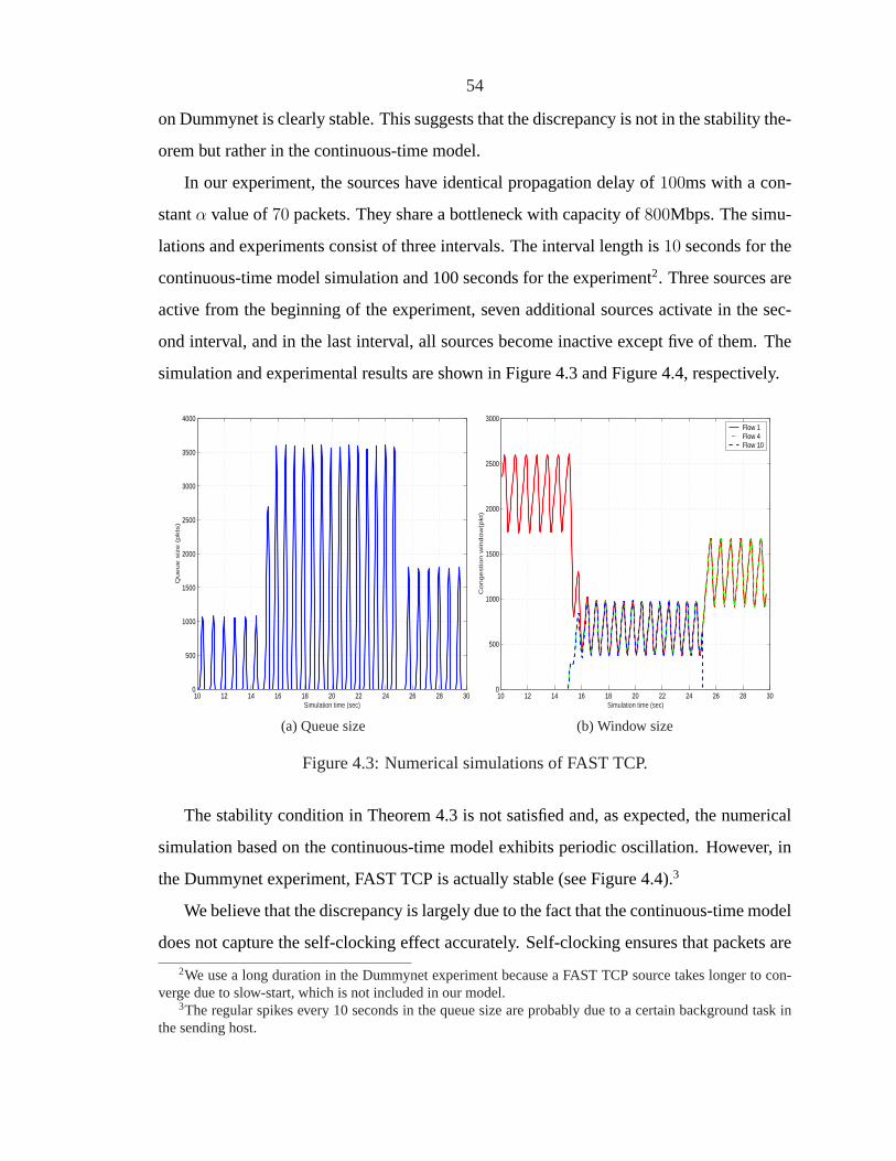
54
on Dummynet is clearly stable. This suggests that the discrepancy is not in the stability the-
orem but rather in the continuous-time model.
In our experiment, the sources have identical propagation delay of100ms with a con-
stantα value of70 packets. They share a bottleneck with capacity of800Mbps. The simu-
lations and experiments consist of three intervals. The interval length is10 seconds for the
continuous-time model simulation and 100 seconds for the experiment2. Three sources are
active from the beginning of the experiment, seven additional sources activate in the sec-
ond interval, and in the last interval, all sources become inactive except five of them. The
simulation and experimental results are shown in Figure 4.3 and Figure 4.4, respectively.
10 12 14 16 18 20 22 24 26 28 300
500
1000
1500
2000
2500
3000
3500
4000
Simulation time (sec)
Queue s
ize (
pkts
)
(a) Queue size
10 12 14 16 18 20 22 24 26 28 300
500
1000
1500
2000
2500
3000
Congestion w
indow
(pkt)
Simulation time (sec)
Flow 1Flow 4Flow 10
(b) Window size
Figure 4.3: Numerical simulations of FAST TCP.
The stability condition in Theorem 4.3 is not satisfied and, as expected, the numerical
simulation based on the continuous-time model exhibits periodic oscillation. However, in
the Dummynet experiment, FAST TCP is actually stable (see Figure 4.4).3
We believe that the discrepancy is largely due to the fact that the continuous-time model
does not capture the self-clocking effect accurately. Self-clocking ensures that packets are
2We use a long duration in the Dummynet experiment because a FAST TCP source takes longer to con-verge due to slow-start, which is not included in our model.
3The regular spikes every 10 seconds in the queue size are probably due to a certain background task inthe sending host.

55
50 100 150 200 2500
100
200
300
400
500
600
700
800
Dum
mynet queue s
ize (
pkt)
Experiment time (sec)
(a) Queue size
50 100 150 200 2500
500
1000
1500
2000
2500
Simulation time (sec)
Congestion w
indow
(pkt)
Flow 1Flow 4Flow 10
(b) Window size
Figure 4.4: Dummynet experiments of FAST TCP.
sent at the same rate as the goodput the source receives, except briefly when the window
size changes. This self-clocking feature can actually help the system approach an equi-
librium. Indeed, for the case of one source for one link, a discrete-event model is used
in [160] to prove that TCP FAST and Vegas are always stable regardless of the feedback
delay. It also provides justification for the discrete-time models in (4.4) and (4.7) based on
the self-clocking feature introduced in the last section.
4.4 Stability analysis with the discrete-time model
We now analyze the stability of this model. We will see that the discrete-time model pre-
dicts that a network of homogeneous sources with the same feedback delay is locally stable
no matter how large the delay is, agreeing with our experimental experience. In the follow-
ing subsection, we study the local stability of FAST TCP using the discrete-time model for
arbitrary networks with feedback delays.

56
4.4.1 Local stability with feedback delay
A network of FAST TCP sources is modelled by equations (4.3), (4.4), and (4.7). This
generalizes the model in [69] by including feedback delay. When local stability is studied,
we ignore all un-congested links (links where prices are zero in equilibrium) and assume
that equality always holds in (4.7).
The main result of this section provides a sufficient condition for local asymptotic sta-
bility in general networks with common feedback delay.
Theorem 4.4. FAST TCP is locally stable for arbitrary networks ifγ ∈ (0, 1] and if all
sources have the same round-trip feedback delayτi = τ for all i.
The stability condition in the theorem does not depend on the value of the feedback
delay, but only on the heterogeneity among them. In particular, when all feedback delays
are ignored,τi = 0 for all i, then FAST TCP is locally asymptotically. This generalizes the
stability result in [69].
Corollary 4.1. FAST TCP is locally asymptotically stable in the absence of feedback delay
for general networks with anyγ ∈ [0, 1).
The rest of this subsection is devoted to the proof of Theorem 4.4.
We applyZ-transform to the linearized system and use the generalized Nyquist criterion
to derive a sufficient stability condition. Define the forward and backwardZ-transformed
routing matricesRf (z) andRb(z) as
(Rf (z))li :=
z−τfli if Rli = 1
0 if Rli = 0and (Rb(z))li :=
z−τbli if Rli = 1
0 if Rli = 0.
The relationτ fli + τ b
li = τi gives
Rb(z) = Rf (z−1) · diag(z−τi). (4.19)
DenoteW (z), Q(z), andP (z) as the correspondingZ-transforms ofδw(t), δq(t), andδp(t)
for the linearized system. Letq andw be the end-to-end queueing delay and congestion

57
window at equilibrium. Linearizing (4.7) yields
∑i
Rli
(δwi(t− τ f
li)
di + qi
− wiδqi(t− τ f
li)
(di + qi)2
)= 0,
where the equality is used in (4.7). The correspondingZ-transform in matrix form is
Rf (z)D−1MW (z)−Rf (z)BQ(z) = 0, (4.20)
where the diagonal matricesB, D, andM are
B := diag
(wi
(di + qi)2
),M := diag
(di
di + qi
), andD := diag(di).
SinceRf (z) is generally not a square matrix, we cannot cancel it in (4.20).
Equation (4.3) is already linear, and the correspondingZ-transform in matrix form is
Q(z) = Rb(z)T P (z). (4.21)
By combining (4.20) and (4.21), we obtain
I −RT
b (z)
Rf (z)B 0
Q(z)
P (z)
=
0
Rf (z)D−1M
W (z).
Solving this equation with block matrix inverse gives the transfer function fromW (z) to
Q(z)
Q(z)
W (z)= RT
b (z)(Rf (z)BRTb (z))−1Rf (z)D−1M.
TheZ-transform of the linearized, congestion window update algorithm is
zW (z) = γ (MW (z)−DBQ(z)) + (1− γ)W (z).
By combining the above equations, we get the open-loop transfer functionL(z) from W (z)

58
to W (z) as
L(z) = − (γ
(M −DBRT
b (z)(Rf (z)BRTb (z))−1Rf (z)D−1M
)+ (1− γ)I
)z−1.
A sufficient condition for local stability can be developed based on the generalized Nyquist
criterion [23, 31]. Since the open-loop system is stable, if we can show that the eigenvalue
loci of L(ejw) does not enclose−1 for ω ∈ [0, 2π), the closed-loop system is stable.
Therefore, if the spectral radius ofL(ejw) is strictly less than 1 forω ∈ [0, 2π), the system
will be stable.
Whenz = ejw, the spectral radii ofL(z) and−zL(z) are the same. Hence, we only
need to study the spectral radius of
J(z) : = γ(M −DBRTb (z)
(Rf (z)BRT
b (z))−1
Rf (z)D−1M + (1− γ)I.
Clearly, the eigenvalues ofJ(z) are dependent onγ. For any givenz = ejω, let the eigen-
values ofJ(z) be denoted byλi(γ), i = 1 . . . N , as functions ofγ ∈ (0, 1]. It is clear
that
|λi(γ)| = |γλi(1) + (1− γ)| ≤ γ|λi(1)|+ (1− γ).
Hence ifρ(J(z)) < 1 for any z = ejω for γ = 1, it will also hold for all γ ∈ (0, 1].
Therefore, it suffices to study the stability condition forγ = 1.
Let µi be theith diagonal entry of matrixM with µi = di/(di + qi). Denoteµmax :=
maxi µi. Since the end-to-end queueing delayqi cannot be zero at equilibrium (otherwise
the rate will be infinitely large), we haveqi > 0 andµmax < 1. The following lemma
characterizes the eigenvalues ofJ(z) with γ = 1.
Lemma 4.2. Whenz = ejω with ω ∈ [0, 2π) andγ = 1, the eigenvalues ofJ(z) have the
following properties:
1. There areL zero eigenvalues with the corresponding eigenvectors as the columns of
matrixM−1DBRTb (z).

59
2. The nonzero eigenvalues have moduli less than1 if τmax− τmin < 1/4, whereτmax =
maxi τi andτmin = mini τi .
Proof: At γ = 1, the matrixJ(z) is
M −DBRTb (z)(Rf (z)BRT
b (z))−1Rf (z)D−1M.
It is easy to check that
J(z)M−1DBRTb (z) = DBRT
b (z)−DBRTb (z) = 0.
SinceM−1DBRTb (z) has full column rank, it consists ofL linearly independent eigenvec-
tors ofJ(z) with corresponding eigenvalue 0. This proves the first assertion.
For the second assertion, suppose thatλ is an eigenvalue ofJ(z) for a givenz. Define
matrixA as
A : = J(z)− λI = (M − λI)−DBRTb (z)(Rf (z)BRT
b (z))−1Rf (z)D−1M,
which is singular by definition. Based on the matrix inversion formula (see, e.g., [62])
(J + EHS)−1 = J−1 − J−1E(H−1 + SJ−1E)−1SJ−1,
if J + EHS is singular, then eitherJ or H−1 + SJ−1E is singular. We can let
J := M − λI, E := −DBRTb (z), H := (Rf (z)BRT
b (z))−1, andS := Rf (z)D−1M.
SinceA = J + EHS is singular, eitherJ = M − λI or H−1 + SJ−1E is singular. The
second term can be reformulated intoRf (z)(B −M(M − λI)−1B)RTb (z).
Case 1:M − λI is singular. SinceM is diagonal, then
0 < λ =di
di + qi
= µi ≤ µmax < 1.
Case 2:Rf (z)(B −M(M − λI)−1B)RTb (z) is singular.
60
It is clear that
B −M(M − λI)−1B = diag(1− µi(µi − λ)−1βi
)= −λdiag
(βi
µi − λ
),
whereβi is the ith diagonal entry of matrixB. Hence,λ = 0 is always an eigenvalue,
which is claimed before. Ifλ is nonzero, it has to be true that
det
(Rf (z)diag
(βi
µi − λ
)RT
b (z)
)= 0. (4.22)
Whenz = ejω, we havez−1 = z. Hence, equation (4.19) can be rewritten as
RTb (z) = diag(z−τi)RT
f (z) = diag(z−τi)R∗f (z).
Substituting the above equation into (4.22) withz = ejω yields
det
(Rf (z)diag
(e−jωτiβi
µi − λ
)R∗
f (z)
)= 0. (4.23)
Therefore, the following formula is also zero
e−j(ωτmax+ψ) det
(Rf (z)diag
(ej(θi+ψ)βi
µi − λ
)R∗
f (z)
)= 0.
whereθi = (τmax − τi)ω, andψ can be any value. Whenτmax − τmin < 1/4, we have
0 ≤ θi = (τmax − τi)ω ≤ π/2.
Suppose that there is a solution such that|λ| ≥ 1. Based on Lemma 4.3, which will be
presented later, there exists aψ s.t. Im(diag(ej(θi+ψ)βi/(µi − λ))
)is a positive diagonal
matrix. Therefore the imaginary part of matrixRf (z)diag(ej(θi+ψ)βi/(µi − λ))
)R∗
f (z)
is positive definite, and the real part is symmetric. From Lemma 4.4 below, it has to be
nonsingular. This contradicts the equation
det
(Rf (z)diag
(ej(θi+ψ)βi
µi − λ
)R∗
f (z)
)= 0.

61
Hence, we have|λ| < 1.
The proof of Theorem 4.4 will be complete after the next two lemmas.
Lemma 4.3. Suppose that0 < µi < 1 and0 ≤ θi < π/2. If |λ| ≥ 1 , there exists aψ such
that
Im
(ej(θi+ψ)βi
µi − λ
)> 0 for i = 1 . . . N.
Proof: See Appendix 4.6.3.
Lemma 4.4. If the real part of a complex matrix is symmetric, and the imaginary part is
positive definite, then the matrix is nonsingular.
Proof: See Appendix 4.6.4.
4.4.2 Global stability for one link without feedback delay
In the absence of feedback delay, when there is only one link, the FAST TCP model can be
simplified into
wi(t + 1) = γ
(diwi(t)
di + q(t)+ αi
)+ (1− γ)wi(t), (4.24)
∑i
wi(t)
di + q(t)≤ c with equality if q(t) > 0, (4.25)
whereq(t) is the queueing delay at the link (subscript is omitted). The main result of this
section proves that the above system (4.24)–(4.25) is globally asymptotically stable and
converges to the equilibrium exponentially fast starting from any initial value.
Theorem 4.5. On a single link, FAST TCP converges exponentially to the equilibrium, in
the absence of feedback delay.
In the rest of this section, we prove the theorem in several steps. The first result is that
after finite stepsK1, equality always holds in (4.25) andq(t) > 0 for any t > K1. Define
62
the normalized congestion window sum asY (t) :=∑
i wi(t)/di. From (4.25), it is clear
thatq(t) > 0 if and only if Y (t) > c.
Lemma 4.5. There existsK1 > 0 such that the following claims are true for allt > K1:
1. q(t) > 0.
2. ν(t + 1) = (1− γ)ν(t) whereν(t) := Y (t)− c−∑i αi/di .
Proof: If initially q(t) = 0, which also meansY (t) ≤ c, from (4.24) we haveY (t + 1) =
Y (t) + γ∑
i αi/di, which linearly increases witht. ThenY (t) > c after some finite steps.
Therefore, there exists aK1 such thatY (t) > c andq(t) > 0 at t = K1.
We will show thatY (t) > c impliesY (t + 1) > c. Henceq(t) > 0 for all t > K1.
Moreover,ν(t) converges exponentially to 0.
SupposeY (t) > c. From∑
i wi(t)/(di + qi(t)) = c, we have
ν(t + 1) =∑
i
wi(t + 1)
di
−∑
i
αi
di
− c,
= (1− γ)∑
i
wi(t)− αi
di
+ γ∑
i
wi(t)
di + q(t)− c,
= (1− γ)
(∑i
wi
di
− c−∑
i
αi
di
)= (1− γ) ν(t).
This proves the second assertion. Moreover it implies
Y (t + 1) = (1− γ)Y (t) + γ
(∑i
αi
di
+ c
).
Hence,Y (t) > c impliesY (t + 1) > c andq(t + 1) > 0. This completes the proof.
For the rest of this subsection, we pick a fixedε with 0 < ε <∑
i αi/di. Define
qmin :=dmin
c
(∑i
αi
di
− ε
), and qmax :=
dmax
c
(∑i
αi
di
+ ε
),
wheredmin := mini di anddmax := maxi di.
Thenq(t) is bounded by these two values after finite steps.

63
Lemma 4.6. There exists a positiveK2 such thatqmin ≤ q(t) ≤ qmax for anyt ≥ K2.
Proof: From Lemma 4.5, after finite stepsK1, ν(t + 1) = (1 − γ)ν(t). Therefore, there
exists aK2 such that|ν(t)| < ε for all t ≥ K2. It implies
∑i
αi
di
<∑
i
wi(t)
di
− c + ε =∑
i
(wi(t)
di
− wi(t)
di + q(t)
)+ ε,
≤∑
i
q(t)wi(t)
dmin(di + q(t))+ ε =
q(t)c
dmin
+ ε.
.
Therefore,
q(t) ≥ dmin
c
(∑i
αi
di
− ε
)= qmin.
The proof forqmax is the same.
Define µi(t) := di/(di + q(t)), and denoteµmax := maxi di/(di + qmin), µmin :=
mini di/(di + qmax). Based on Lemma 4.6, we have1 > µmax ≥ µi(t) > µmin > 0 for any
t ≥ K2. Define
ηi(t) :=wi(t)− αi
αidi
− 1
q(t), (4.26)
and denoteηmax(t) := maxi ηi(t), ηmin(t) := mini ηi(t). We will show that the window
update for sourcei is proportional toηi(t), and the system is at equilibrium if and only if
all ηi(t) are zero. The next lemma gives bounds onηi(t).
Lemma 4.7. There exist two positive numbersδ1 andδ2 such that for allt ≥ K2
ηmax(t) > −δ1(1− γ)t and ηmin(t) < δ2(1− γ)t.
Proof: From (4.26), it is easy to check thatY (t + 1) − Y (t) = −γν(t). By Lemma 4.5,
whent ≥ K2 we have
Y (t + 1)− Y (t) = −γν(t) ≤ γ(1− γ)t−K2|ν(K2)| = κ(1− γ)t, (4.27)

64
whereκ := γ(1− γ)−K2|ν(K2)|.The update of sourcei’s congestion window is
wi(t + 1)− wi(t) = γ
(diwi(t)
di + q(t)+ αi − wi(t)
)=
γq(t)
di + q(t)
(αidi
q(t)− (wi(t)− αi)
),
= −γαidiq(t)
di + q(t)
(wi(t)− αi
αidi
− 1
q(t)
)= −γαiq(t)µi(t)ηi(t).
Chooseδ1 large enough such thatδ1Nγαminqminµmin/dmax > κ whereαmin := mini αi.
We now proveηmax(t) > −δ1(1 − γ)t for all t ≥ K2 by contradiction. Suppose that
there is a timet ≥ K2 such thatηmax(t) ≤ −δ1(1 − γ)t. Then all theηi(t) are negative,
which implies
Y (t + 1)− Y (t) =∑
i
(wi(t + 1)− wi(t))/di =∑
i
−γαiq(t)µi(t)ηi(t)/di,
≥ N(−ηmax)γαminqminµmin/dmax,
≥ δ1N(1− γ)tγαminqminµmin/dmax > κ(1− γ)t.
This contradicts equation (4.27), which proves the claim. The proof forηmin(t) is similar.
DefineL(t) as:
L(t) := ηmax(t)− ηmin(t). (4.28)
The following lemma implies that the difference between differentηi(t) goes to zero expo-
nentially fast.
Lemma 4.8. There are two positive numbersδ3 andδ4, such that fort ≥ K2 we have
1. L(t) ≥ 0.
2. L(t + 1) ≤ (1− γ + γµmax)L(t) + δ3(1− γ)t.
3. L(t) ≤ δ4(1− γ + γµmax)t.
Proof: See Appendix 4.6.5.

65
Lemma 4.9. Bothηmax(t) andηmin(t) exponentially converge to zero.
Proof: Whent ≥ K2, combining Lemma 4.7 and Lemma 4.8 yields an upper bound for
ηmax(t),
ηmax(t) = L(t) + ηmin(t) ≤ δ4(1− γ + γµmax)t + δ2(1− γ)t.
The lower bound ofηmax is−δ1(1−γ)t ≤ ηmax(t). Since both the upper and lower bounds
of ηmax(t) converge to zero exponentially fast, it exponentially goes to zero. The proof for
ηmin(t) is similar.
Proof of Theorem 4.5: The system is at equilibrium if and only ifwi(t) = wi(t + 1) for
all i. This is equivalent toηi(t) = 0 for all i because of the equation
wi(t + 1)− wi(t) = −γαiq(t)µi(t)ηi(t).
Since bothηmax(t) andηmin(t) converge to zero exponentially from any initial value, the
system converges to the equilibrium defined byηi(t) = 0 globally.
4.5 Conclusion
We have introduced the traditional continuous-time model for FAST TCP. We analyze its
stability for general networks. We prove that the FAST TCP system is globally stable
without feedback delay. When the feedback delays are present, a sufficient condition is
provided for local stability. However, there are certain inconsistencies between this model
and our experiments, which maybe due to the self-clocking effects.
We present a new discrete-time link model that fully captures the effect of self-clocking.
Using this discrete-time model, we have derived a sufficient condition for local asymptotic
stability for general networks in the presence of feedback delay. The condition states that
the system is stable if the difference among delays of the sources is small. This implies, in
particular, that a network with homogeneous sources is always stable, consistent with our
66
experimental experience so far. We also prove that FAST TCP is globally stable on a single
link in the absence of feedback delay.
This work can be extended in several ways. First, the condition for local asymptotic
stability derived appears more restrictive than our experiments suggest. Moreover, we have
also found scenarios where predictions of the discrete-time model disagree with experi-
ment. These discrepancies should be clarified. Second, it will be interesting to extend
the global stability analysis to general networks with feedback delays. Finally, the new
model and the analysis techniques here can be applied to analyze other congestion control
algorithms.
4.6 Appendix
4.6.1 Proof of Lemma 4.1
The FAST TCP model (4.1, 4.3, 4.5, 4.2, and 4.6) can be linearized into
δqi(t) =∑
l
Rliδpl(t− τ bli), δxi(t) =
δwi(t)
di + qi
− wiδqi(t)
(di + qi)2,
δwi(t) = γ
(−qiδwi(t)
di + qi
− diwiδqi(t)
(di + qi)2
), δyl(t) =
∑i
Rliδxi(t− τ fli),
δpl(t) = δyl(t)/cl,
wherewi andqi are the equilibrium values. Sinceτi = τ fli + τ b
li for all link l on the path of
sourcei, the following equation holds
RTb (s) = diag(e−τis)RT
f (−s). (4.29)
67
The Laplace transform of the linearized system in matrix form is
Q(s) = Rb(s)T P (s),
X(s) = D1W (s)−BQ(s, )
sW (s) = γ ((DD1 − I)W (s)−DBQ(s)) ,
Y (s) = Rf (s)X(s),
sP (s) = D3Y (s),
where the diagonal matrices are
D := diag(di) , D1 := diag
(1
di + qi
),
B := diag
(wi
(di + qi)2
), D3 := diag
(1
cl
).
The open-loop transfer function fromP (s) to P (s) can be derived based on the above
equations as
1
sD3Rf (s)
(γDD1(sI − γ(DD1 − I))−1 + 1
)D2R
Tb (s).
By using the fact thatTi = di + qi, xi = wi/Ti and (4.29), we can simplify the open loop
transfer functionL(s) into (4.16).
4.6.2 Proof of Theorem 4.3
It is sufficient to show that the eigenvalues of the open-loop transfer function do not encircle
−1 in the complex plain fors = jω, ω ≥ 0 when the condition is satisfied. Since both
X andΛ(s) are diagonal matrices, by using the similar technique in [24], it is not difficult
to check that whens = jω, the set of eigenvalues ofL(s) is same as that ofL(jω) =
Λ(s)RT (−jω)R(jω) except for some zero eigenvalues whereR(jω) is defined as
R(jω) := diag(1√cl
)Rf (jω)diag(√
xi).

68
Following the argument of [152], we study the convex hull as a function ofjω formed by
N Nyquist trajectories. More specifically, the spectrum ofL(jω) satisfies
σ(L(jω)) = σ(Λ(s)RT (−jω)R(jω)
)⊆ ρ
(RT (−jω)R(jω)
)· co(0 ∪ {Λi(jω)}) ,
wherei = 1 . . . N , co(·) denotes the convex hull, and
Λi(jω) :=e−jωTi
jωTi
jωTi + γTi
jωTi + γqi
,
where theτi is replaced withTi sinceτi = Ti at equilibrium. Similar to [24], the spectral
radius ofRT (−jω)R(jω) is less thanM , which is the maximal number of links in the path
of any source,M = maxi
∑l Rli. It implies
σ(L(jω)) ⊆ M · co(0 ∪ {Λi(jω), i = 1 . . . N}) .
Therefore a sufficient condition for local stability is thatMΛi(jω) does not encircle−1 for
any i.
It is a standard control theory result that the largest phase lag of(jωTi + γTi)/(jωTi +
γqi) is produced whenωTi =√
γTi · γqi , which is
∠j√
γTi · γqi + γTi
j√
γTi · γqi + γqi
= − tan−1 1− qi/Ti
2√
qi/Ti
.
The above equation yields
∠Λi(jω) ≥ −ωTi − π
2− tan−1 1− qi/Ti
2√
qi/Ti
.
Suppose that at frequencyωi the phase lag ofΛi(jω) is−π. Hence,
−π = Λi(jωi) ≥ −ωiTi − π
2− tan−1 1− qi/Ti
2√
qi/Ti
.

69
Based on (4.18) we have
ωiTi ≥ φ for i = 1 . . . N.
It is easy to check that the magnitude ofΛi(jω) is a decreasing function ofω. Therefore,
M |Λi(jωi)| ≤ M |Λi(jφ
Ti
)| = M
φ
√φ2 + γ2T 2
i
φ2 + γ2q2i
≤ M
φ
√φ2 + γ2T 2
max
φ2 + γ2q2min
< 1,
andMΛ(jωi) can not encircle−1. Based on the above argument, the system is locally
stable if (4.17 ) is satisfied.
4.6.3 Proof of Lemma 4.3
O
Z
Re
Im
A B
λ
λ
Figure 4.5: Illustration of Lemma 4.3.
Proof: There is a complex plane in Figure 4.5. Let the pointsA, B, andλ represent the
value ofµmin, µmax, andλ, respectively.Z is the intersection of segmentAλ and the unit
circle, andλ stands for the complex conjugate ofλ.
Let φi ∈ [0, 2π) be the phase of1/(µi − λ). Clearly, φi ∈ [0, π) if Im(λ) ≤ 0,
andφi ∈ (π, 2π) otherwise. Denoteφmax := maxi φi andφmin := mini φi, then0 ≤φmax − φmin ≤ π. Since everyµi is in the range[µmin, µmax], it is easy to check that every

70
φi is in the range formed by the phases of1/(µmin − λ) and1/(µmax − λ). This implies
φmax − φmin ≤ |∠ 1
µmin − λ− ∠ 1
µmax − λ| = ∠AλB = ∠AλB < ∠OZB < π/2.
Let ε > 0 be small enough such thatφmax − φmin < π/2 − ε. Choosingψ = −φmin + ε
gives us
∠ej(ψ+θi)βi
µi − λ= φi + ψ + θi,
= φi − φmin + ε + θi, (greater than 0)
< φmax − φmin + ε + π/2 < π.
The fact that its phase is in(0, π) implies that
Im
(ej(ψ+θi)βi
µi − λ
)> 0.
4.6.4 Proof of Lemma 4.4
Suppose thatA = Ar + jAi whereAr = ATr andAi is positive definite. IfA is singular,
there exists a nonzero vectorv such thatAv = 0. Suppose thatv = α + jβ. ThenAv = 0
gives
Arα− Aiβ = 0, (4.30)
Arβ + Aiα = 0. (4.31)
Multiplying βT to equation (4.30) yields
βT Arα = βT Aiβ ≥ 0. (4.32)

71
Multiplying αT to equation (4.31) gives us
αT Arβ = −αT Aiα ≤ 0. (4.33)
SinceβT Arα = αT ATr β = αT Arβ, both (4.32) and (4.33) must hold with equality. This
means that bothα andβ are zero. It contradicts the assumption thatv is nonzero.
4.6.5 Proof of Lemma 4.8
It is obvious thatL(t) ≥ 0 because of its definition in (4.28). We start with the update of
ηi(t)
ηi(t + 1)− ηi(t) =wi(t + 1)− wi(t)
αidi
− 1
q(t + 1)+
1
q(t),
= −γαiq(t)µi(t)ηi(t)
αidi
− 1
q(t + 1)+
1
q(t),
= −γq(t)ηi(t)
di + q(t)− 1
q(t + 1)+
1
q(t),
= −γ(1− µi(t))ηi(t)− 1
q(t + 1)+
1
q(t).
For simplicity, we letai(t) := 1 − γ + γµi(t) and denoteamax := 1 − γ + γµmax, then
ai(t) ≤ amax. This definition simplifies the above equation into
ηi(t + 1) = ai(t)ηi(t)− 1
q(t + 1)+
1
q(t). (4.34)
By comparing equation (4.34) for sourcei andj, we obtain
ηi(t + 1)− ηj(t + 1) = ai(t)ηi(t)− aj(t)ηj(t). (4.35)
Without loss of generality, suppose that at timet + 1, the largest and smallest values ofη
are achieved at sourcesi andj, respectively. This assumption implies
L(t + 1) = ηi(t + 1)− ηj(t + 1).

72
The upper bound ofL(t+1) is derived by considering the following three cases separately.
Case 1:ηi(t) andηj(t) have different signs. It is easy to see that
L(t + 1) = ai(t)ηi(t)− aj(t)ηj(t) ≤ amax(ηi(t)− ηj(t)),
≤ amax(ηmax(t)− ηmin(t)) = amaxL(t).
Case 2:Bothηi(t) andηj(t) are positive. It yields
L(t + 1) = ai(t)µi(t)ηi(t)− aj(t)ηj(t) ≤ amaxηmax(t),
= amaxL(t) + amaxηmin(t) ≤ amaxL(t) + amaxδ2(1− γ)t,
≤ amaxL(t) + δ3(1− γ)t,
where the last step is choosingδ3 larger thanamaxδ2.
Case 3:Bothηi(t) andηj(t) are negative. The proof is similar to that for Case 2.
Summarizing all the above cases, we have provedL(t+1) ≤ amaxL(t)+ δ3(1−γ)t for
all t ≥ K2. Denoteb := 1 − γ, then1 > amax > b ≥ 0. For anyt ≥ K2, an upper bound
of L(t) is
L(t) ≤ amaxL(t− 1) + δ3bt−1 ≤ at−K2
max L(K2) + δ3(bt−1 + bt−2amax + · · ·+ bK2at−K2−1
max ),
=
(a−K2
max L(K2)− δ3bK2a−K2
max
b− amax
)at
max +δ3
b− amax
bt.
Note that the coefficient ofbt is negative. By choosingδ4 as the coefficient ofatmax, we get
L(t) ≤ δ4atmax = δ4(1− γ + γµmax)
t.

73
Chapter 5
Cross-Layer Optimization in TCP/IPNetworks
5.1 Introduction
Recent studies have shown that any TCP congestion control algorithm can be interpreted
as carrying out a distributed primal-dual algorithm over the Internet to maximize aggregate
utility, and a user’s utility function is defined by its TCP algorithm, see, e.g., [80, 97, 116,
107, 101, 88, 96] for unicast, [75, 30] for multi-cast, and [98, 79, 138] for recent surveys
and further references. All of these works assume that routing is given and fixed at the
timescale of interest, and TCP, together with active queue management (AQM), attempts
to maximize aggregate utility over source rates. In this chapter, we study the cross-layer
utility maximization at the timescale of route changes.
We focus on the situation where a single minimum-cost route (shortest path) is selected
for each source-destination pair. This models IP routing in the current Internet within an
Autonomous System using common routing protocols such as OSPF [119]1 or RIP [56].
Routing is typically updated at a much slower timescale than TCP–AQM. We model this
by assuming that TCP and AQM converge instantly to equilibrium after each route update
to produce source rates and “congestion prices” for that update period. These congestion
prices may represent delays or loss probabilities across network links. They determine
the next routing update in the case of dynamic routing, similar to the system analyzed in
1Even though OSPF implements a shortest-path algorithm, it allows multiple equal-cost paths to be uti-lized. Our model ignores this feature.

74
[48]. Thus TCP–AQM/IP forms a feedback system where routing interacts with congestion
control in an iterative process. We are interested in the equilibrium and stability properties
of this iterative process. To simplify notation, we will henceforth use TCP–AQM/IP and
TCP/IP interchangeably.
Here are our main results. In the case of pure dynamic routing, i.e., when link costs are
the congestion prices generated by TCP–AQM, it turns out that we can interpret TCP/IP
as a distributed primal-dual algorithm to maximize aggregate utility overbothsource rates
(by TCP–AQM) and routes (by IP) if TCP/IP converges. We consider the problem, and its
Lagrangian dual, of maximizing utility over source rates and over routing that use only a
singlepath for each source-destination pair. Unlike the TCP-AQM problem or the multi-
path routing problem that are convex optimizations with no duality gap, the single path
TCP/IP problem is non-convex and generally has a duality gap. Equilibrium of the TCP/IP
system exists if and only if this problem has no duality gap. In this case, TCP/IP equilibrium
solves both the primal and the dual problem. Moreover, it incurs no penalty for not splitting
traffic across multiple paths: optimal single-path routing achieves the same aggregate utility
as optimal multi-path routing. Multi-path routing can achieve a strictly higher utility only
when there is a duality gap between the single-path primal and dual problems, but in this
case, the TCP/IP iteration does not even have an equilibrium, let alone solving the utility
maximization problem.
Even when the single-path problem has no duality gap and TCP/IP has an equilibrium,
the equilibrium is generally unstable under pure dynamic routing. It can be stabilized by
adding a sufficiently large static component to the definition of link cost. The existence
and characterization of TCP/IP equilibrium when the link costs are not pure congestion
prices, however, are open problems. To proceed, we specialize to a ring network with a
common destination and demonstrate an inevitable tradeoff between utility maximization
and routing stability (Section 5.5). Specifically, we show that the TCP/IP system over the
special ring network is indeed unstable when link costs are pure prices. It can be stabilized
by adding a static component to the link cost, but at the expense of a reduced utility in
equilibrium. The loss in utility increases with the weight on the static component. Hence,
while stability requires a small weight on prices, utility maximization favors a large weight.

75
We present numerical results to validate these qualitative conclusions in a general network
topology. These results also suggest that routing instability can reduce aggregate utility to
less than that achievable by (the necessarily stable) pure static routing.
Indeed we show that if the link capacities are optimally provisioned, thenpure static
routing is enough to maximize utility even for general networks (Section 5.6). Moreover,
it is optimal within the class of multi-path routing: again, there is no penalty at optimality
in not splitting traffic across multiple paths.
Finally, we discuss some implications and limitations of these results (Section 5.7).
5.2 Related work
Our goal is to understand equilibrium and stability issues in cross-layer optimization of
TCP/IP networks. Another approach to joint routing and congestion control is to allow
multi-path routing, i.e., a source can transmit its data along multiple paths to its destination.
In this formulation, a source’s decision is decomposed into two: how much traffic to send
(congestion control) and how to distribute it over the available paths (multi-path routing
or load balancing) in order to maximize aggregate utility. This has been analyzed in, e.g.,
[46, 80, 74]. The general intuition is that, for each source-destination pair, only paths with
the minimum, and hence equal, “congestion prices” will be used, and this minimum price
determines the total source rate as in the single-path case. In contrast to TCP/IP networks,
this formulation assumes that both decisions operate on the same timescale. However, it
provides an upper bound to the problem TCP/IP attempts to solve (see Section 5.4).
The multi-path problem is equivalent to the multicommodity flow problem which has
been extensively studied; see, e.g., [1, 13]. The standard formulation is to maximize aggre-
gate throughput, corresponding to a common and linear utility function. It is then a linear
program and therefore can be solved in polynomial time, though there are combinatorial
algorithms for this class of problems that are more efficient. Recently, fast approxima-
tion algorithms and their competitive ratios have been developed for network flow, and
other, problems, e.g., [130, 48, 7]. Since the multi-path problem upper bounds the TCP/IP
problem, the work on network flow problems provides insight to the performance limit of

76
TCP/IP. There are however differences. First, our single-path routing problem is NP-hard
(see Section 5.4) and generally has a duality gap, whereas the network flow problem is gen-
erally a linear program that is in P and has no duality gap. Second, the utility functions that
correspond to common TCP algorithms are strictly concave whereas they are typically lin-
ear, in fact, identity, functions in network flow problems. Third, the algorithms developed
for network flow problems are typically centralized and therefore cannot model TCP/IP
iterations or be carried out in a large network where they must be decentralized.
Instability of single-path routing is not surprising as it is well known that stability gen-
erally requires that the relative weight on the dynamic (traffic-sensitive) component of the
link cost be small. Indeed, our conclusions are similar to those reached in [12, 103] that
study the same ring network for routing stability using different link costs. Here, since the
dynamic component is the dual-optimal price for the utility maximization problem com-
puted by TCP–AQM, this implies a tradeoff between routing stability and utility maxi-
mization.
5.3 Model
In general, we use small letters to denote vectors, e.g.,x with xi as itsith component;
capital letters to denote matrices, e.g.,H,W,R, or constants; e.g.,L,N, K i; and script
letters to denote sets of vectors or matrices, e.g.,Ws,Wm,Rs,Rm. Superscript is used to
denote vectors, matrices, or constants pertaining to sourcei, e.g.,yi, wi, H i, K i.
A network is modelled as a set ofL uni-directional links with finite capacitiesc =
(cl, l = 1, . . . , L), shared by a set ofN source-destination pairs, indexed byi (we will also
refer to the pair simply as “sourcei”). There areKi acyclic paths for sourcei represented
by aL×K i 0-1 matrixH i where
H ilj =
1, if path jof sourcei uses linkl
0, otherwise.
Let Hi be the set of all columns ofH i that represents all the available paths toi under

77
single-path routing. Define theL×K matrixH as
H = [H1 . . . HN ],
whereK :=∑
i Ki, andH defines the topology of the network.
Let wi be aK i × 1 vector where thejth entry represents the fraction of sourcei on its
jth path such that
wij ≥ 0 ∀j, and 1T wi = 1,
where1 is a vector of an appropriate dimension with the value1 in every entry. We require
wij ∈ {0, 1} for single-path routing and allowwi
j ∈ [0, 1] for multi-path routing. Collect
the vectorswi, i = 1, . . . , N , into aK ×N block-diagonal matrixW . LetWs be the set of
all such matrices corresponding to single-path routing defined as
{W |W = diag(w1, . . . , wN) ∈ {0, 1}K×N , 1T wi = 1 }.
Define the corresponding setWm for multi-path routing as
{W |W = diag(w1, . . . , wN) ∈ [0, 1]K×N , 1T wi = 1 }. (5.1)
As mentioned above,H defines the set of acyclic paths available to each source and rep-
resents the network topology.W defines how the sources load balance across these paths.
Their product defines aL × N routing matrixR = HW that specifies the fraction ofi’s
flow at each linkl. The set of all single-path routing matrices is
Rs := { R | R = HW,W ∈ Ws }, (5.2)
and the set of all multi-path routing matrices is
Rm := { R | R = HW,W ∈ Wm }. (5.3)
78
The difference between single-path routing and multi-path routing is the integer constraint
onW andR. A single-path routing matrix inRs is an 0-1 matrix
Rli =
1, if link l is in a path of sourcei
0, otherwise.
A multi-path routing matrix inRm is one whose entries are in the range[0, 1]
Rli
> 0, if link l is in a path of sourcei
= 0, otherwise.
The path of sourcei is denoted byri = [R1i . . . RLi]T , the ith column of the routing
matrixR.
We consider the situation where TCP–AQM operates at a faster timescale than routing
updates. We assume asinglepath is selected for each source-destination pair that mini-
mizes the sum of the link costs in the path, for some appropriate definition of link cost. In
particular, traffic is not split across multiple paths from the source to the destination even
if it is available. This models, for example, IP routing within an Autonomous System. We
focus on the timescale of the route changes and assume TCP–AQM is stable and converges
instantly to equilibrium after a route change. As in [96], we will interpret the equilibria of
various TCP and AQM algorithms as solutions of a utility maximization problem defined
in [80]. Different TCP algorithms solve the same prototypical problem (5.4) with different
utility functions [96, 101].
Specifically, suppose each sourcei has a utility functionUi(xi) as a function of its total
transmission ratexi. We assumeUi is strictly concave increasing (which is the case for
common TCP algorithms [96]). LetR(t) ∈ Rs be the (single-path) routing in periodt. Let
the equilibrium ratesx(t) = x(R(t)) and pricesp(t) = p(R(t)) generated by TCP–AQM
in periodt, respectively, be the optimal solutions of the constrained maximization problem
maxx≥0
∑i
Ui(xi) s. t. R(t)x ≤ c, (5.4)

79
and its Lagrangian dual
minp≥0
∑i
maxxi≥0
(Ui(xi)− xi
∑
l
Rli(t)pl
)+
∑
l
clpl. (5.5)
The prices,pl(t), l = 1, . . . , L, are measures of congestion, such as queueing delays or loss
probabilities [96, 101]. We assume the link costs in periodt are
dl(t) = apl(t) + bτl, (5.6)
wherea ≥ 0, b ≥ 0, andτl > 0 are constants. Based on these costs, each source computes
its new routeri(t + 1) ∈ Hi individually that minimizes the total cost on its path
ri(t + 1) = arg minri∈Hi
∑
l
dl(t)ril . (5.7)
In (5.6),τl are traffic insensitive components of the link costdl(t), e.g.,τl = 1/cl. If τl
represent the fixed propagation delays across linksl andpl(t) the queueing delays at link
l, thendl(t) represent total delays across linkl. The protocol parametersa andb determine
the responsiveness of routing to network traffic:a = 0 corresponds to static routing,b = 0
corresponds to purely dynamic routing, and the larger the ratio ofa/b, the more responsive
routing is to network traffic. As we will see below, they determine whether an equilibrium
exists and whether it is stable, and the achievable utility at equilibrium.
An equivalent way to specify the TCP–AQM/IP system as a dynamical system, at the
timescale of route changes, is to replace (5.4)–(5.5) by their optimality conditions. The
routing is updated according to
ri(t + 1) = arg minri∈Hi
∑
l
(apl(t) + bτl)ril , for all i, (5.8)

80
wherep(t) andx(t) are given by
∑
l
Rli(t)pl(t) = U ′i(xi(t)) for all i (5.9)
∑i
Rli(t)xi(t)
≤ cl if pl(t) ≥ 0
= cl if pl(t) > 0for all l (5.10)
x(t) ≥ 0, p(t) ≥ 0. (5.11)
This set of equations describe how the routingR(t), ratesx(t), and pricesp(t) evolve.
Note thatx(t) andp(t) depend only onR(t) through (5.9)–(5.11), implicitly assuming that
TCP–AQM converges instantly to an equilibrium given the new routingR(t).
We say that(R∗, x∗, p∗) is an equilibrium of TCP/IPif it is a fixed point of (5.4)–
(5.7), or equivalently, (5.8)–(5.11), i.e., starting from routingR∗ and associated(x∗, p∗),
the above iterations yield(R∗, x∗, p∗) in the subsequent periods.
5.4 Equilibrium of TCP/IP
In this section, we study the condition under which TCP/IP as modelled by (5.4)–(5.7) or
(5.8)–(5.11) has an equilibrium and characterize the equilibrium as the optimal solution
of an optimization problem. Since (5.8)–(5.11) is a system of mixed integer nonlinear
inequalities, characterization of its equilibrium, even the basic question of existence and
uniqueness, is in general difficult to determine. The case of pure dynamic routing,a > 0
andb = 0, is the simplest and most instructive.
We completely characterize the case of pure dynamic routing,a > 0 andb = 0 in this
section. Without loss of generality, we seta = 1 in (5.7) and (5.8) whenb = 0.
Consider the joint optimization problem
maxR∈Rs
maxx≥0
∑i
Ui(xi) s. t.Rx ≤ c, (5.12)

81
and its Lagrangian dual
minp≥0
∑i
maxxi≥0
(Ui(xi)− xi min
ri∈Hi
∑
l
Rlipl
)+
∑
l
clpl, (5.13)
whereri is the ith column ofR with ril = Rli. While (5.4)–(5.5) maximize utility over
source rates only, problem (5.12) maximizes utility over both rates and routes. While (5.4)
is a convex program without duality gap, problem (5.12) is non-convex because the variable
R is discrete and generally has a duality gap.2 The interesting feature of the dual problem
(5.13) is that the maximization overR takes the form of minimum-cost routing with prices
p generated by TCP–AQM as link costs. This suggests that TCP/IP might turn out to be
a distributed algorithm that attempts to maximize utility, with proper choice of link costs.
This is indeed true when equilibrium of TCP/IP exists.
Theorem 5.1.Under pure dynamic routing, that is,a = 1 andb = 0.
1. An equilibrium(R∗, x∗, p∗) of TCP/IP exists if and only if there is no duality gap
between (5.12) and (5.13).
2. In this case, the equilibrium(R∗, x∗, p∗) is a solution of (5.12) and (5.13).
Hence, one can regard the layering of TCP and IP as a decomposition of the utility
maximization problem over source rates and routes into a distributed and decentralized
algorithm, carried out on two different timescales, in the sense that an equilibrium of the
TCP/IP iteration (5.8)–(5.11), if it exists, solves (5.12) and (5.13). An equilibrium may not
exist. Even if it does, it may not be stable–an issue we address in Section 5.5.
Example 1: Duality gap
A simple example, where there is a duality gap and equilibrium of TCP/IP does not exist,
consists of a single source-destination pair connected by two parallel links each of capacity
1, as shown in Figure 5.2 (takeN = 1). Clearly, under pure dynamic single-path routing,
equilibrium of TCP/IP does not exist, because the TCP/IP iteration (5.8)–(5.11) will choose
2The nonlinear constraintRx ≤ c can be converted into a linear constraint–see proof of Theorem 5.2–sointeger constraint onR is the real source of difficulty.
82
one of the two routes in each period to carry all traffic. TCP–AQM will generate positive
price for the chosen route and zero price for the other route, so that in the next period, the
other route will be selected, and the cycle repeats. The proof that there is a duality gap
between the primal problem (5.12) and the dual problem (5.13) is given in Appendix 5.8.1
(takeN = 1). Intuitively, either path is optimal (both for primal and for dual problem). For
the primal problem the optimal rate isx∗ = 1, constrained by link capacity, whereas for
the dual problem, the optimal rate isx∗ = 2, primal infeasible. Hence the primal optimal
value isU(1), strictly less than the dual optimal value ofU(2).
The duality gap is a measure of “cost of not splitting”. To elaborate, define the La-
grangian [14, 104]
L(R, x, p) =∑
i
(Ui(xi)− xi
∑
l
Rlipl
)+
∑
l
clpl.
The primal (5.12) and dual (5.13) can then be expressed respectively as
Vsp = maxR∈Rs,x≥0
minp≥0
L(R, x, p)
Vsd = minp≥0
maxR∈Rs,x≥0
L(R, x, p).
If we allow sources to distribute their traffic among multiple paths available to them, then
the corresponding problems for multi-path routing are
Vmp = maxR∈Rm,x≥0
minp≥0
L(R, x, p)
Vmd = minp≥0
maxR∈Rm,x≥0
L(R, x, p). (5.14)
Theorem 5.2.The relations among these four problems areVsp ≤ Vsd = Vmp = Vmd.
According to Theorem 5.1, TCP/IP has an equilibrium exactly when there is no dual-
ity gap in the single-path utility maximization, i.e., whenVsp = Vsd. Theorem 5.2 then
says that in this case, there is no penalty in not splitting the traffic, i.e., single-path routing
performs as well as multi-path routing,Vsp = Vmp. Multi-path routing achieves a strictly

83
higher utilityVmp precisely when TCP/IP has no equilibrium, in which case the TCP/IP it-
eration (5.8)–(5.11) cannot converge, let alone solving the single-path utility maximization
problem (5.12) or (5.13). In this case the problem (5.12) and its dual (5.13) do not charac-
terize TCP/IP, but their gap measures the loss in utility in restricting routing to single-path
and is of independent interest.
Even though minimum-cost routing is polynomial, it is shown in [153] that single-path
utility maximization is NP-hard. This is not surprising since, e.g., a related problem on
load balancing on a ring has been proved to be NP-hard in [29].
Theorem 5.3.The primal problem (5.12) is NP-hard.
Theorem 5.3 shows that the general problem (5.12) is NP-hard by reducing all instances
of the integer partition problem to some instances of the primal problem (5.12). Theorem
5.2 however implies that the sub-class of the utility maximization problems with no duality
gap are polynomial-time solvable, since they are equivalent to multi-path problems that are
concave programs and hence polynomial-time solvable. It is a common phenomenon for
sub-classes of NP-hard problems to have polynomial-time algorithms. Informally, the hard
problems are those with nonzero duality gap.
The rest of this section is devoted to the proofs for Theorems 5.1–5.3. We will first
prove Theorem 5.2. Then we show that an equilibrium of TCP/IP must solve the dual
problem (5.13). This together with Theorem 5.2 implies Theorem 5.1. Finally, we present
a proof for Theorem 5.3.
Proof of Theorem 5.2. The inequality follows from the weak duality theorem [14]. We
now proveVsd = Vmd andVmp = Vmd. We formulateVsd as
Vsd = minp≥0
maxR∈Rs,x≥0
(∑i
Ui(xi)− pT Rx
)+ pT c,
= minp≥0
maxx≥0
(∑i
Ui(xi)− minW∈Ws
pT HWx
)+ pT c,

84
whereR = HW with W ∈ Ws from (5.2). Similarly, from (5.3) we have
Vmd = minp≥0
maxx≥0
(∑i
Ui(xi)− minW∈Wm
pT HWx
)+ pT c.
Define functionsfs(x, p) andfm(x, p) as
fs(x, p) := minW∈Ws
pT HWx, fm(x, p) := minW∈Wm
pT HWx.
In order to show thatVsd = Vmd, we only need to show thatfs(x, p) = fm(x, p). Clearly
fs(x, p) ≥ fm(x, p) sinceWs ⊆ Wm. From (5.1), noting thatW = diag(wi), we have
fm(x, p) = minW
pT HWx
s. t. 1T wi = 1, 0 ≤ wij ≤ 1.
Since this is a linear programming for givenx andp, at least one of the optimal points lies
on the boundary, i.e.,wij = 0 or 1 for all i andj, and hence is inWs ⊆ Wm. Such a point
solves bothfs(x, p) andfm(x, p), i.e.,fs(x, p) = fm(x, p).
To showVmd = Vmp, transformVmp into a convex optimization with linear constraints,
which hence has no duality gap; see, e.g., [14]. Now,Vmp is equivalent to the problem
maxR∈Rm,x≥0
∑i
Ui(xi) s.t. Rx ≤ c. (5.15)
Note that this is not a convex program since the feasible set specified byRx ≤ c is generally
not convex. Define theKi × 1 vectorsyi in terms of the scalarxi and theKi × 1 vectors
wi as the new variables
yi = xiwi. (5.16)
The mapping from(xi, wi) to yi is one-to-one: the inverse of (5.16) isxi = 1T yi and
wi = yi/xi. Now change the variables in (5.15) and (5.14) from(W,x) to y by substituting

85
xi = 1T yi andRx = HWx = Hy into (5.15) and (5.14). We obtain an equivalent problem
maxy≥0
∑i
Ui(1T yi) s.t. Hy ≤ c
and its Lagrangian dual. This is a convex program with linear constraint and hence has no
duality gap. This provesVmp = Vmd.
Proof of Theorem 5.1. It is easy to show that optimal solutions exist for both the primal
problem (5.12) and its dual (5.13), so the issue is whether there is a duality gap. We will
prove the theorem in two steps. First, given an equilibrium(R, x, p) of TCP/IP, we will
show that it solves both the primal (5.12) and the dual (5.13), and hence there is no duality
gap. Then, given a solution(R∗, x∗, p∗) of the primal and the dual problems, we will show
that it is an equilibrium of TCP/IP.
Step 1: Necessity.Let (R, x, p) be an equilibrium of TCP/IP, i.e., a fixed point of (5.4)–
(5.7) witha = 1, b = 0. Then
pT ri = minri∈Hi
pT ri for all i, (5.17)
(p, x) = arg minp≥0
maxx≥0
(∑i
U(xi)− pT Rx
)+ pT c, (5.18)
whereri are theith columns of routing matrixR ∈ Rs.3 We will show that(R, x, p) solves
the dual problem (5.13). Then, since the dual problem (5.13) upper bounds the primal
problem (5.12) by Theorem 5.2, andR ∈ Rs is a single-path routing and hence primal
feasible,(R, x, p) also solves the primal (5.12).
To show that(R, x, p) solves the dual problem, we use the fact that the dual problem
has an optimal solution, denoted by(R∗, x∗, p∗) and show that both achieve the same dual
3One can exchange the order of min and max in (5.18) since givenR, there is no duality gap inmaxx≥0
∑i Ui(xi) s. t. Rx ≤ c.

86
objective value, i.e.,L(R, x, p) = L(R∗, x∗, p∗). Now
(p∗, x∗, R∗) = arg minp≥0
maxx≥0
(∑i
U(xi)− minR∈Rs
pT Rx + pT c
). (5.19)
Let
f(p) := maxx≥0
(∑i
U(xi)− pT Rx
)+ pT c,
g(p) := maxx≥0
(∑i
U(xi)− minR∈Rs
pT Rx
)+ pT c.
Then (5.18) impliesf(p) = minp≥0 f(p) and (5.19) impliesg(p∗) = minp≥0 g(p). Since
R ∈ Rs, we have
f(p) ≤ g(p) for all p ≥ 0,
and hence
f(p) = minp≥0
f(p) ≤ minp≥0
g(p) = g(p∗).
On the other hand
f(p) = maxx≥0
∑i
U(xi)− pT Rx + pT c
= maxx≥0
∑i
U(xi)−∑
i
xi
(pT ri
)+ pT c
= maxx≥0
∑i
U(xi)−∑
i
xi
(minri∈Hi
pT ri
)+ pT c
= g(p)
≥ g(p∗),
where the third equality follows from (5.17). Therefore,f(p) = g(p∗) = g(p) and
L(R, x, p) = L(R∗, x∗, p∗). Moreover,(R, x, p) is an optimal solution of the dual prob-
lem.
87
Step 2: Sufficiency. Assume that there is no duality gap and(R∗, x∗, p∗) is an optimal
solution for both the primal problem (5.12) and its dual (5.13). We claim that it is also an
equilibrium of (5.4)–(5.7) witha = 1 andb = 0, i.e., we need to show that
(p∗)T (ri)∗ = minri∈Hi
(p∗)T ri, (5.20)
(p∗, x∗) = arg minp≥0
maxx≥0
L(R∗, x, p) = arg maxx≥0
minp≥0
L(R∗, x, p), (5.21)
where(ri)∗ are theith columns ofR∗. The second equality in (5.21) follows from the fact
that there is no duality gap for the TCP–AQM problem.
Since(R∗, x∗, p∗) solves the dual problem (5.13), the optimal routing matrixR∗ satisfies
(5.20) by the saddle point theorem [14]. But(R∗, x∗, p∗) also solves the primal problem
(5.12). In particular,(x∗, p∗) solves the utility maximization problem over source rates and
its Lagrangian dual, withR∗ as the routing matrix, i.e.,(x∗, p∗) satisfies (5.21).
Proof of Theorem 5.3.We describe a polynomial time procedure that reduces an instance
of integer partition problem [47, pp. 47] to a special case of the primal problem. Given a
set of integersc1, . . . , cN , the integer partition problem is to find a subsetA ⊂ {1, . . . , N}such that
∑i∈A
ci =∑
i 6∈A
ci.
Given an instance of the integer partition problem, consider the network in Figure 5.1, with
N sources at the root, two relay nodes, andN receivers, one at each of theN leaves. The
two links from the root to the relay nodes have a capacity of∑
i ci/2 each, and the two links
from each relay node to receiveri have a capacity ofci. All receivers have the same utility
function that is increasing. The routing decision for each source is to decide which relay
node to traverse. Clearly, maximum utility of∑
i Ui(ci) is attained when each receiveri
receives at rateci, from exactly one of the relay nodes, and the links from the root to the
two relay nodes are both saturated. Such a routing exists if and only if there is a solution to
the integer partition problem.

88
ic
2
1ic
2
1
1c
2c
Nc
Nc 1
c
2c
Figure 5.1: Network to which integer partition problem can be reduced.
Comment: The case ofb > 0 for general network is completely open. Ifa = 0 and
b > 0, routingR(t) = R, for all t, is the static minimum-cost routing withτl as the link
costs. An equilibrium(R, x(R), p(R)) always exists in this case. Even thoughR minimizes
routing cost and(x(R), p(R)) solves (5.4)–(5.5), it is not known if(R, x(R), p(R)) jointly
solves any optimization problem.
For the case ofa > 0 andb > 0, even the existence of equilibrium is unknown for
general networks. In the following section, we will study the dynamics of TCP/IP under
the assumption that such an equilibrium of TCP/IP exists.
5.5 Dynamics of TCP/IP
Theorem 5.1 suggests using pure congestion pricesp(t) generated by TCP–AQM as link
costs. In this case, an equilibrium of TCP/IP, when it exists, maximizes aggregate utility
over both rates and routes. We show in this section however that the equilibrium may not
be unstable. Routing can be stabilized by including a strictly positive traffic-insensitive
(static) component in link costs (b > 0), but at a reduced achievable utility. There thus
seems to be an inevitable tradeoff between achievable utility and routing stability.
To make this precise, we start with analysis of a special ring network with a common
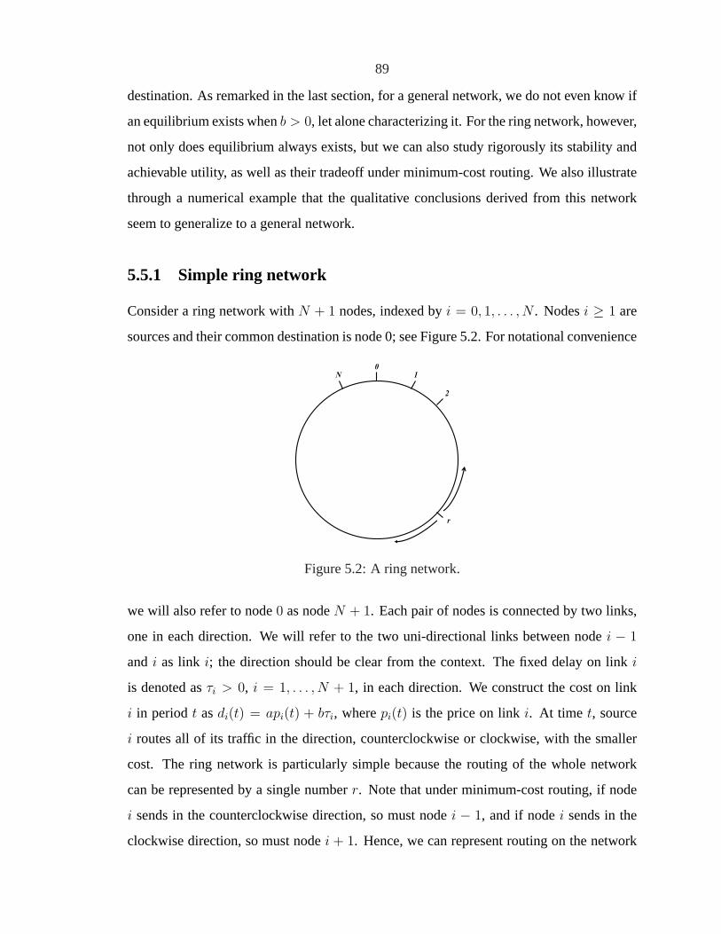
89
destination. As remarked in the last section, for a general network, we do not even know if
an equilibrium exists whenb > 0, let alone characterizing it. For the ring network, however,
not only does equilibrium always exists, but we can also study rigorously its stability and
achievable utility, as well as their tradeoff under minimum-cost routing. We also illustrate
through a numerical example that the qualitative conclusions derived from this network
seem to generalize to a general network.
5.5.1 Simple ring network
Consider a ring network withN + 1 nodes, indexed byi = 0, 1, . . . , N . Nodesi ≥ 1 are
sources and their common destination is node 0; see Figure 5.2. For notational convenience
r
2
0
N 1
Figure 5.2: A ring network.
we will also refer to node0 as nodeN + 1. Each pair of nodes is connected by two links,
one in each direction. We will refer to the two uni-directional links between nodei − 1
and i as link i; the direction should be clear from the context. The fixed delay on linki
is denoted asτi > 0, i = 1, . . . , N + 1, in each direction. We construct the cost on link
i in periodt asdi(t) = api(t) + bτi, wherepi(t) is the price on linki. At time t, source
i routes all of its traffic in the direction, counterclockwise or clockwise, with the smaller
cost. The ring network is particularly simple because the routing of the whole network
can be represented by a single numberr. Note that under minimum-cost routing, if node
i sends in the counterclockwise direction, so must nodei − 1, and if nodei sends in the
clockwise direction, so must nodei + 1. Hence, we can represent routing on the network

90
by r ∈ {0, . . . , N} with the interpretation that nodes1, . . . , r send in the counterclockwise
direction and nodesr + 1, . . . , N send in the clockwise direction.
For this special case, we now show that the duality gap is trivial, that minimum-cost
routing based just on prices (b = 0) indeed solves the primal and dual problems as Theorem
5.1 guarantees, but that the equilibrium is unstable. Using a continuous model, we then
show that routing can be stabilized if the weightb on the fixed delay is nonzero and the
weighta on price is small enough. The maximum achievable utility however decreases with
smallera. There is thus an inevitable tradeoff between utility maximization and routing
stability.
5.5.2 Utility and stability of pure dynamic routing
Suppose all sourcesi have the same utility functionU(xi), and all links have the same
capacity ofc = 1 unit. We assume thatU is strictly concave increasing and differen-
tiable. Then at any time, only link 1, in the counterclockwise direction, and linkN + 1,
in the clockwise direction, can be saturated and have strictly positive price. The utility
maximization problem (5.12) reduces to the following simple form
maxr∈{0,...,N}
maxxi
∑i
U(xi) (5.22)
subject tor∑
i=1
xi ≤ 1, andN∑
i=r+1
xi ≤ 1. (5.23)
When routing isr, nodesi = 1, . . . , r see pricep1(r) on their paths while nodesi =
r + 1, . . . , N see pricepN+1(r) on their paths. Since these ratesxi(r) and pricespi(r) are
primal and dual optimal, they satisfy [97]
U ′(xi(r)) = p1(r) for i = 1, . . . , r, (5.24)
U ′(xi(r)) = pN+1(r) for i = r + 1, . . . , N. (5.25)
This implies thatx1(r) = · · · = xr(r) andxr+1(r) = · · · = xN(r).
It is easy to see that the optimal routingr∗ 6= 0 or N . Hence both constraints are active

91
at optimality, implying that (from (5.23))
x1(r) = · · · = xr(r) = 1r, (5.26)
xr+1(r) = · · · = xN(r) = 1N−r
. (5.27)
The problem (5.22)–(5.23) thus becomes
maxr∈{1,...,N−1}
r U
(1
r
)+ (N − r) U
(1
N − r
).
Dividing the objective function byN and using the strict concavity ofU , we have
r
NU
(1
r
)+
N − r
NU
(1
N − r
)≤ U
(2
N
),
with equality if and only ifr = N/2. This implies that the optimal routing is
r∗ := bN/2c (5.28)
and the maximum utility is
V ∗ :=
⌊N
2
⌋U
(1
bN/2c)
+
⌈N
2
⌉U
(1
dN/2e)
, (5.29)
wherebyc is the largest integer less or equal toy anddye is the smallest integer greater or
equal toy.
It can be shown that there is no duality gap for the ring network considered here
whenN is even, by verifying that routingr∗ in (5.28), ratesxi(r∗) in (5.27), and prices
p1(r∗), pN+1(r
∗) in (5.24)–(5.25) are indeed primal-dual optimal.4 WhenN is odd, there
is generally a duality gap due to integral constraint onr; see Appendix 5.8.1 for a proof.
This duality gap disappears in the convexified problem when routing is allowed to take
real value in[0, N ], a model we consider in the next subsection. This suggests that TCP
together with minimum-cost routing based on prices can potentially maximize utility for
4This also follows from Theorem 5.1 and the fact thatr = N/2 is by symmetry the equilibrium routingwhenN is even.

92
this ring network. We next show, however, that minimum-cost routing based only on prices
is unstable.
Given routingr, we can combine (5.24)–(5.25) and (5.27) to obtain the pricesp1(r) and
pN+1(r) on links 1 andN + 1
p1(r) = U ′(
1
r
)andpN+1(r) = U ′
(1
N − r
). (5.30)
The path cost for nodei in the counterclockwise direction is
D−(i; r) =i∑
j=1
bτj + ap1(r) = b
i∑j=1
τj + aU ′(
1
r
), (5.31)
and the path cost in the clockwise direction is
D+(i; r) =N+1∑
j=i+1
bτj + apN+1(r) = b
N+1∑j=i+1
τj + aU ′(
1
N − r
). (5.32)
In the next period, each nodei will choose the counterclockwise or clockwise direction
accordingly asD−(i; r) or D+(i; r) is smaller. Definef(r) as
f(r) := max {i | D−(i; r) ≤ D+(i; r)}. (5.33)
Then the resulting routing satisfies the recursive relation
r(t + 1) =
0 if D−(1; r(t)) > D+(1; r(t))
N if D−(N ; r(t)) < D+(N ; r(t))
f(r(t)) otherwise.
Theorem 5.4. If b = 0 anda > 0, then, starting from any routingr(0) except the equilib-
rium N/2 whenN is even, the subsequent routing oscillates between 0 andN .

93
Proof. For anyr(0) ∈ {0, . . . , N}, we have
D−(1; r(0))−D+(1; r(0)) = D−(N ; r(0))−D+(N ; r(0)),
= a
(U ′
(1
r(0)
)− U ′
(1
N − r(0)
)).
If N is even, thenN/2 is the unique equilibrium routing that solvesD−(i; N/2) = D+(i; N/2).
Supposer(0) 6= N/2. If r(0) > N/2, then1/r(0) < 2/N < 1/(N − r(0)). SinceU ′ is
strictly decreasing,U ′(1/r(0)) > U ′(1/(N − r(0)) and henceD−(1; r(0)) > D+(1; r(0))
andr(1) = 0. Similarly, if r(0) < N/2, thenD−(N ; r(0)) < D+(N ; r(0)) andr(1) = N .
Hencer oscillates between 0 andN henceforth.
Even though purely dynamic routing based on prices(b = 0) maximizes utility, The-
orem 5.4 says that it is unstable. We will henceforth, without loss of generality, setb = 1
and consider the effect ofa on utility maximization and stability.
5.5.3 Maximum utility of minimum-cost routing
As mentioned above, the duality gap for the ring network we consider is of a trivial kind
that disappears when integer constraint on routing is relaxed. For the rest of this section,
we consider a continuous model where every point on the ring is a source. A point on the
ring is labelled bys ∈ [0, 1], and the common destination is the point0 (or equivalently 1).
The utility maximization problem becomes
maxr∈[0,1]
maxx(·)
∫ 1
0
U(x(u))du (5.34)
subject to∫ r
0
x(u)du ≤ 1, and∫ 1
r
x(u)du ≤ 1. (5.35)
As in the discrete case, both constraints are active at optimality, and hence the problem
reduces to
maxr∈(0,1)
rU
(1
r
)+ (1− r)U
(1
1− r
),

94
which, by concavity, yields the optimal routingr∗ and maximum utilityV ∗
r∗ =1
2, and V ∗ = U(2). (5.36)
To see that there is no duality gap, note that the problem (5.34)–(5.35) is equivalent to
maxr∈[0,1]
maxx−,x+≥0
rU(x−) + (1− r)U(x+),
subject to rx− ≤ 1, (1− r)x+ ≤ 1.
Define the Lagrangian as
L(r, x−, x+, p−, p+) = rU(x−) + (1− r)U(x+) + p−(1− rx−) + p+(1− (1− r)x+).
It is easy to verify that
r∗ =1
2, x−∗ = x+∗ = 2, p−∗ = p+∗ = U ′(2) (5.37)
are primal-dual optimal and there is no duality gap; see Appendix 5.8.2.
We now look at the maximum utility achievable by the equilibrium of minimum-cost
routing. Let the delay froms to the destination in the counterclockwise direction be
T (s) :=
∫ s
0
τ(u)du,
and the delay in the clockwise direction be
T (1)− T (s) =
∫ 1
s
τ(u)du,
whereτ(u), u ∈ [0, 1], is given. Here,τ(u) corresponds to link cost in the discrete model.
Given routingr ∈ [0, 1], the price in the counterclockwise direction isU ′(1/r), and the
price in the clockwise direction isU ′(1/(1− r)). Then the cost of sources in the counter-
95
clockwise direction is
D−(s; r) = T (s) + aU ′(
1
r
), (5.38)
and the cost in the clockwise direction is
D+(s; r) = T (1)− T (s) + aU ′(
1
1− r
). (5.39)
A routing r is in equilibrium if the costs of sourcer in both directions are the same.
Definition 5.1. A routingr is called anequilibrium routingif D−(r; r) = D+(r; r). It is
denoted byra or r(a).
By definition,ra is the solution of
g(r) := 2T (r)− T (1) + a
(U ′
(1
r
)− U ′
(1
1− r
))= 0. (5.40)
Sinceg(0) < 0, g(1) > 0 andg′(r) > 0, the equilibriumra is in (0, 1) and is unique. Given
a routingr, its utility is
V (r) := rU
(1
r
)+ (1− r)U
(1
1− r
).
The maximum utility achieved by minimum-cost routing, with parametera, is thenV (ra) ≤V (r∗) = V ∗.
The next result implies thatra varies betweenr0 andr∗ and converges monotonically to
r∗ asa →∞. As a result, the lossV ∗ − V (ra) ≥ 0 in utility also approaches0 asa →∞.
Denote the interval in which1/ra and1/(1− ra) vary asI := [2, 1/ min{r0, 1− r0}].
Theorem 5.5.SupposeU ′′ exists and is bounded onI. For all a ≥ 0, |ra − r∗| is a strictly
decreasing function ofa. Moreover, asa →∞, |ra − r∗| andV ∗ − V (ra) approach 0.
Proof. The equation (5.40) defines the equilibrium routingr(a) := ra as an implicit func-

96
tion of a. By the implicit function theorem,r′(a) satisfies
1
r′(a)
[U ′
(1
1− ra
)− U ′
(1
ra
)]= 2τ(ra)− a
r2a
U ′′(
1
ra
)− a
(1− ra)2U ′′
(1
1− ra
).
The right-hand side is positive sinceU is strictly concave. Hencer′(a) has the same sign
as the term in the square bracket, i.e., sinceU ′ is decreasing,
r′(a) =
> 0 if ra < r∗
< 0 if ra > r∗
= 0 if ra = r∗
. (5.41)
This implies that|ra − r∗| is a strictly decreasing function ofa; see Figure 5.3.
Hence|ra − r∗| converges to a limit asa → ∞. SinceU ′′ is bounded on the closed
intervalI, so isU ′. Hence, from (5.40), we must have
U ′(1/ra)− U ′(1/(1− ra)) → 0, or U ′(1/ lima→∞
ra) = U ′(1/(1− lima→∞
ra)).
SinceU ′ is strictly decreasing, this implies thatlima→∞ ra = 1− lima→∞ ra = r∗.
To show thatV ∗ − V (ra) ≥ 0 also converges to 0, note thatV ′(r∗) = 0 and hence we
have, by Taylor expansion,
V (ra)− V ∗ =1
2V ′′(u)(ra − r∗)2
for someu betweenra andr∗. Here
V ′′(u) =1
u3U ′′
(1
u
)+
1
(1− u)3U ′′
(1
1− u
)≥ − 2µ
(min{r0, 1− r0})3
whereµ is the upper bound ofU ′′ on I. Hence
0 ≤ V ∗ − V (ra) ≤ µ(ra − r∗)2
(min{r0, 1− r0})3.
Since|ra − r∗| → 0, the proof is complete.
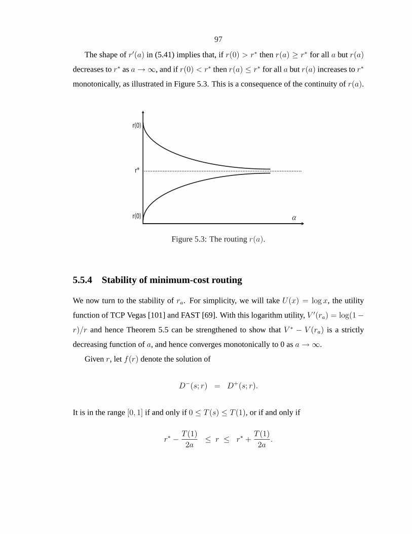
97
The shape ofr′(a) in (5.41) implies that, ifr(0) > r∗ thenr(a) ≥ r∗ for all a but r(a)
decreases tor∗ asa →∞, and ifr(0) < r∗ thenr(a) ≤ r∗ for all a butr(a) increases tor∗
monotonically, as illustrated in Figure 5.3. This is a consequence of the continuity ofr(a).
r(0)
r*
r(0)
Figure 5.3: The routingr(a).
5.5.4 Stability of minimum-cost routing
We now turn to the stability ofra. For simplicity, we will takeU(x) = log x, the utility
function of TCP Vegas [101] and FAST [69]. With this logarithm utility,V ′(ra) = log(1−r)/r and hence Theorem 5.5 can be strengthened to show thatV ∗ − V (ra) is a strictly
decreasing function ofa, and hence converges monotonically to 0 asa →∞.
Givenr, let f(r) denote the solution of
D−(s; r) = D+(s; r).
It is in the range[0, 1] if and only if 0 ≤ T (s) ≤ T (1), or if and only if
r∗ − T (1)
2a≤ r ≤ r∗ +
T (1)
2a.

98
We will assume thatminu∈[0,1] τ(u) > 0. ThenT−1 exists and
f(r) = T−1
(1
2(T (1) + a)− ar
). (5.42)
The routing iteration is
r(t + 1) = [f(r(t))]10 , (5.43)
where[r]10 = max{0, min{1, r}}.
Definition 5.2. The equilibrium routingra is (globally) stable, if starting from any routing
r(0), r(t) defined by (5.42)–(5.43) converges tora ast →∞.
Example 2: Uniform τ
Suppose delay is uniform on the ring,τ(u) = τ for all u ∈ [0, 1], so thatT (r) = rτ . From
(5.40), the equilibrium routing is
ra =1
2= r∗, ∀a ≥ 0
coinciding with the utility-maximizing routingr∗.
Supposea < τ . Then the routing iteration becomes
r(t + 1) =1
2τ(τ + a)− a
τr(t) = f(r(t)).
Since|f(s)− f(r)| = (a/τ)|s− r| < |s− r|, f(r) is a contraction mapping and hencera
is globally stable for all0 ≤ a < τ .
Hence for the uniform delay case, adding a static component to link cost stabilizes
routing provided the weight on prices is smaller than link delay. Moreover, the static com-
ponent does not lead to any loss in utility (ra = r∗). The stability condition generalizes to
the general delay case. The following theorem says that ifa is smaller than the minimum
“link delay,” thenra is globally stable; ifa is bigger than the maximum “link delay,” then it

99
is globally unstable (diverge from any initial routing exceptra); otherwise, it may converge
or diverge depending on initial routing.
Theorem 5.6.The stability is affected by parametera such that
1. If a < minu∈[0,1] τ(u) thenra is globally stable.
2. Supposea ≥ T (1). Then there existsr < ra < r such that
(a) If r(0) = r or r(0) = r then subsequent routings oscillate betweenr andr.
(b) If r(0) < r or r(0) > r then subsequent routings after a finite number of
iterations oscillate between 0 and 1.
(c) If r < r(0) < r thenr(t) converges tora provideda < minu∈(r,r) τ(u).
3. If a > maxu∈[0,1] τ(u) then starting from any initial routingr(0) 6= ra, subsequent
routings after a finite number of iterations oscillate between 0 and 1.
Proof. 1. We show that the routing iteration (5.43) is a contraction mapping ifa <
minu∈[0,1] τ(u). Now
∣∣[f(s)]10 − [f(r)]10∣∣ ≤ |f(s)− f(r)| ,
=
∣∣∣∣T−1
(T (1) + a− 2as
2
)− T−1
(T (1) + a− 2ar
2
)∣∣∣∣ ,
=
∣∣∣∣1
T ′(u)(as− ar)
∣∣∣∣ ,
≤ a
minu∈[0,1] τ(u)|s− r|,
for someu betweenr and s, by the mean value theorem. Henceh(r) is a contraction
mapping and starting from anyr(0) ∈ [0, 1], r(t) converges exponentially tora.
2. Defineh(r) = (T (1) + a)/2− ar. The routing iteration can be written as
T (r(t + 1)) = [h(r(t))]10. (5.44)

100
Define the following sequences
a0 = 0, b0 = T (0),
an+1 = h−1(bn), bn+1 = T (an+1).
Note that(an, n ≥ 0) is a routing sequence going backward in time. The following lemma
is proved in the appendix, following [103].
Lemma 5.1. LetTa = T (ra) = h(ra). Then
0 = a0 < a2 < · · · < ra < · · · < a3 < a1 < 1,
T (0) = b0 < b2 < · · · < Ta < · · · < b3 < b1 < T (1).
Since the sequences are monotone, the lemma implies that there arer andr with 0 <
r < ra < r < 1 such that
limn→∞
a2n = r, and limn→∞
a2n+1 = r.
By continuity ofT andh, we have
T (r) = h(r), and T (r) = h(r).
This implies that starting fromr(0) = r or r(0) = r, the subsequent routings oscillate
betweenr andr.
To show the second claim, supposer(0) < r. Specifically, supposea2n−2 < r(0) < a2n
for somen. If h(r(0)) > T (1) (possible sincea ≥ T (1)), thenr(1) = 1 and subsequent
routings oscillate between 0 and 1. Otherwise, from (5.44),r(0) = h−1(T (r(1))), and
hencea2n−2 < h−1(T (r(1))) < a2n. Sinceh is strictly decreasing, we haveb2n−1 <
T (r(1)) < b2n−3 by definition ofbn. Hence, sinceT is strictly increasing,a2n−1 < r(1) <
a2n−3. The same argument then shows thata2n−4 < r(2) < a2n−2. Hence we have shown
thatr(0) < a2n impliesr(2) < a2n−2. This proves the second claim. The proof of the third

101
claim follows the same argument of part 1.
3. By the mean value theorem, we have, for allα, α′ in [0, 1],
|h−1(T (α))− h−1(T (α′))| =T ′(u)
a|α− α′|,
for someu betweenα andα′. Hence the iteration map
an+1 = h−1(T (an))
is a contraction provideda > maxu∈[0,1] τ(u). This implies that the sequence(an, n ≥ 0)
converges and, sincera is the unique fixed point ofh−1(T (·)), r = r = ra. The assertion
then follows from part 2(b).
5.5.5 General network
It is difficult to derive an analytical bound ona to guarantee routing stability or to compute
optimal routing for general networks. In this section, we present numerical results to illus-
trate that the intuition from the simple ring network analyzed in the previous subsections
extends to general topology.
We generate a random network based on Waxman’s algorithm [159]. The nodes are
uniformly distributed in a two-dimensional plane. The probability that a pair of nodesu, v
are connected is given by
Prob(u, v) = α exp
(d(u, v)
βL
),
where the maximum probabilityα > 0 controls connectivity,β ≤ 1 controls the length of
the edges with a largerβ favoring longer edges,d(u, v) is the Euclidean distance between
nodesu andv, andL is the maximum distance between any two nodes. In our example, we
set the number of nodesN = 30, α = 0.8, β = 0.3, which generated 90 bidirectional links;
see Figure 5.4. The fixed delayτl of each linkl is randomly chosen according to a uniform
distribution over [100, 400]ms. The link capacities are randomly chosen from the interval

102
0 0.1 0.2 0.3 0.4 0.5 0.6 0.7 0.8 0.9 10
0.1
0.2
0.3
0.4
0.5
0.6
0.7
0.8
0.9
1
x
y
random network with N=30,α=0.8,β=0.3
Figure 5.4: A random network.
[1000, 4000] packets/sec, also with uniform distribution. There are 60 flows on the network
with randomly chosen source and destination nodes. Routing on this network is computed
using the Bellman-Ford minimum-cost algorithm, with link costdl(t) = τl +apl(t) in each
update periodt, on a slower timescale than congestion control. In each routing periodt,
we first solve the link prices based on the current routing, using the gradient projection
algorithm of [97]. We iterate the source algorithm to update rates and the link algorithm to
update prices, until they converge. The link prices are then used to compute the minimum-
cost for the next period.
We measure the performance of the scheme at differenta by the sum of all of the
source’s utilities. If the routing is stable (at smalla), the aggregate utility is computed using
the equilibrium routing. Otherwise, the routing oscillates and the time-averaged aggregate
utility is used. The result is shown in Figure 5.5.
As expected, whena is small, routing is stable and the aggregate utility increases with
a, as in the ring network analyzed in Section 5.5.3 (Theorem 5.5). Whena < 4, the static
delayτl dominates the link cost, and the routes computed withdl(t) remain the same as
with static routing (a = 0), and hence the aggregate utility is independent ofa. Routing

103
100
101
102
392
394
396
398
400
402
404
406
408
410
412
α value
ag
gre
ga
te u
tilit
y
Figure 5.5: Aggregate utility as a function ofa for random network
becomes unstable at arounda = 10. Even though the time-averaged utility continues to
rise after routing instability sets in, eventually it peaks and drops to a level less than the
utility achievable by the necessarily stable static routing.
5.6 Resource provisioning
Results in the previous sections show that even though an equilibrium of TCP/IP, when
it exists, maximizes utility under pure dynamic routing, it can be unstable and hence not
attainable by the TCP/IP system. In this section, we show that if the link capacities are op-
timally provisioned, however, purestaticrouting is enough to maximize utility. Moreover,
it is optimal even within the class of multi-path routing: again, there is no penalty in not
splitting traffic across multiple paths.
Suppose it costsαl > 0 amount to provision a unit of capacity at linkl, and letα = (αl,
for all l) be the vector of unit costs. For instance, a longer link may have a largerαl. The
total capacity cost over the entire network isαT c. Suppose the budget for provisioning the
capacity isB. Consider the problem of optimally selecting capacities, routing, and source

104
rates to maximize utility
maxc≥0
maxR∈Rm
maxx≥0
∑i
Ui(xi), (5.45)
subject to Rx ≤ c, (5.46)
αT c ≤ B. (5.47)
whereUi are concave increasing utility functions. Note thatR ranges inRm and hence
multi-path routing is allowed. This problem may arise when optical lightpaths can be
dynamically reconfigured at a connection timescale.
Theorem 5.7.SupposeU ′i(xi) > 0 for all i andxi ≥ 0. At optimality,
1. There is an optimal solution(c∗, R∗, x∗) whereR∗ ∈ Rs is a single-path routing.
2. Moreover,R∗ is pure static routing usingαl as link costs.
3. R∗x∗ = c∗, i.e., there is no slack capacity.
4. αT c = B, i.e., there is no slack in budget.
5. Link prices generated by TCP–AQM are proportional to the provisioning costs,p∗ =
γ∗α for someγ∗ > 0.
Proof. It is easy to show the existence of an equilibrium. Define the Lagrangian of (5.45)-
(5.47) as
L(c, R, x, p, γ) =∑
i
Ui(xi)− pT (Rx− c)− γ(αT c−B).
At optimality, the KKT condition holds: there existp∗ ≥ 0 andγ∗ ≥ 0 such that
U′(x∗i ) = (R∗)T p∗, (5.48)
p∗ = γ∗α, (5.49)
(p∗)T (R∗x∗ − c∗) = 0, (5.50)
γ∗(αT c∗ −B) = 0. (5.51)

105
From (5.49), we obtain the last claim in the theorem. Moreover, (5.49) andU ′i(x
∗i ) > 0
imply that γ∗ > 0 andp∗l > 0 for all l, sinceα > 0. Hence, from (5.50) and (5.51),
equality holds in (5.46) and (5.47), proving the third and fourth claims.
To prove the first two claims, express the routing matrixR asR = HW whereW ∈Wm. Using the equalities in (5.46) and (5.47) to eliminatec, we can transform the utility
maximization problem (5.45)–(5.47) into:
maxW∈Wm
maxx≥0
∑i
Ui(xi),
subject to∑
i
(αT H iwi
)xi = B,
whereW =diag(wi). SinceUi is nondecreasing and both the objective and the constraints
above are separable ini, in order to maximize utility,wi should be chosen to be a solution
of
minwi
αT H iwi,
subject to 1T wi = 1, 0 ≤ wij ≤ 1.
Since this is a linear program, there exists an optimal point on the boundary. Hence there
is an optimalW ∗ ∈ Ws, i.e., minimum-cost single-path routing usingαl as link costs is
optimal.
5.7 Conclusion
Given a routing, TCP-AQM can be interpreted as a distributed primal-dual algorithm over
the Internet to maximize aggregate utility over source rates. In this chapter, we study
whether TCP-AQM together with IP (modelled by minimum-cost routing) can maximize
utility over both source rates and routing, on a slower time scale. We show that we can
indeed interpret TCP/IP asattemptingto maximize utility in the sense that its equilibrium,
if it exists, solves the utility maximization problem and its dual, provided congestion prices
generated by TCP-AQM are used as link costs. TCP/IP equilibrium exists if and only if

106
there is no penalty in not splitting traffic across multiple paths. Even if equilibrium exists,
however, TCP/IP with pure dynamic routing can be unstable. Specializing to a special ring
network, we show that routing is indeed unstable when link costs are congestion prices. It
can be stabilized by adding a static component to the definition of link cost, but the static
component reduces the achievable utility. There thus seems to be an inevitable tradeoff
between routing stability and utility maximization, for a given set of link capacities. We
show, however, that if link capacities are optimally provisioned, then pure static (and hence
stable) routing is sufficient to maximize utility even for general networks, and link costs
are proportional to the provisioning costs. Moreover single-path routing can achieve the
same utility as multi-path routing. Hence, one can regard the layering of TCP and IP as
a decomposition of the utility maximization problem over source rates and routes into a
distributed and decentralized algorithm, carried out on different time scales, at least when
network capacities are well provisioned.
5.8 Appendix
5.8.1 Proof of duality gap
We prove that there is generally a duality gap between the primal problem (5.22)–(5.23)
and its dual whenN is odd.
It is easy to see that the primal optimal routing is
r∗ =N − 1
2, or
N + 1
2.
Suppose without loss of generality thatr∗ = (N − 1)/2 (the other case is similar). Then,
the source rates are
x1 = · · · = xr∗ =2
N − 1, and xr∗+1 = · · · = xN =
2
N + 1
107
yielding a primal objective value of
N − 1
2U
(2
N − 1
)+
N + 1
2U
(2
N + 1
)
= N
{ (1
2− 1
N
)U
(2
N − 1
)+
(1
2+
1
N
)U
(2
N + 1
)}
< NU
(2
N
),
where the last inequality follows from the strict concavity ofU . We now show that the
right-hand side is the optimal dual objective value, and hence there is a duality gap.
The dual problem of (5.22)–(5.23) is (e.g., [97])
minp1,pN+1≥0
(N∑
i=1
maxxi
φ(xi, p1, pN+1) + (p1 + pN+1)
),
whereφ(xi, p1, pN+1) = U(xi)−xi min{p1, pN+1}. First, note that the minimizing(p1, pN+1)
must satisfyp1 = pN+1, for otherwise, if (say)p1 < pN+1, then the dual objective value is
N∑i=1
maxxi
(U(xi)− xip1) + (p1 + pN+1)
and can be reduced by decreasingpN+1 to p1. Hence the dual problem is equivalent to
minp≥0
N∑i=1
maxxi
(U(xi)− xi p) + 2p. (5.52)
Let p∗ denote the minimizer andx∗i = xi(p∗) = x(p∗) =: x∗ denote the corresponding
maximizers (they are equal for alli by symmetry). Then we have
U ′(x∗) = p∗. (5.53)
Differentiating the objective function in (5.52) with respect top and setting it to zero, we
have
0 = N(U ′(x∗)x′(p∗)− p∗x′(p∗)− x∗) + 2. (5.54)

108
Using (5.53), we havex∗ = 2/N, and hence the minimum dual objective value is
N(maxx∗
U(x∗)− x∗ p∗) + 2p∗ = NU
(2
N
)
as desired.
5.8.2 Proof of primal-dual optimality
We prove that the solution given by (5.37) is primal-dual optimal using the saddle-point
theorem (e.g., [14, pp. 427]). Clearly,(r∗, x−∗, x+∗) is primal feasible and(p−∗, p+∗)
is dual feasible. We now show that(r∗, x−∗, x+∗, p−∗, p+∗) is a saddle point, i.e., for all
(r, x−, x+, p−, p+). Now
L(r, x−, x+, p−∗, p+∗) ≤ L(r∗, x−∗, x+∗, p−∗, p+∗) ≤ L(r∗, x−∗, x+∗, p−, p+).
For the right inequality, substituting(r∗, x−∗, x+∗) from (5.37) intoL(r∗, x−∗, x+∗, p−, p+)
to get, for all(p−, p+),
L(r∗, x−∗, x+∗, p−, p+) = U(2).
But U(2) = L(r∗, x−∗, x+∗, p−∗, p+∗), establishing the right inequality. For the left in-
equality, denotingp∗ := p−∗ = p+∗, from (5.37) we have
L(r, x−, x+, p−∗, p+∗) = rU(x−) + (1− r)U(x+)− (rx− + (1− r)x+)p∗ + 2p∗
≤ U(y)− yp∗ + 2p∗ (concavity ofU), (5.55)
with y := rx− + (1− r)x+, where equality holds if and only ifx− = x+ sinceU is strictly
concave. Notice that the right-hand side is maximized overy if and only if y satisfies
U ′(y) = p∗. This implies thaty = x−∗ = x+∗ = 2 sinceU ′ is strictly monotonic. Substitute
y = 2 into (5.55) yields, for all(r, x−, x+),
L(r, x−, x+, p−∗, p+∗) ≤ U(2)

109
as desired, sinceU(2) = L(r∗, x−∗, x+∗, p−∗, p+∗).
5.8.3 Proof of Lemma 5.1
We will prove the lemma by induction. Note thatb0 < Ta implies thata1 = h−1(b0) >
h−1(Ta) = ra. Sincea ≥ T (1) andh(1) < 0, a1 = h−1(b0) < 1 (see Figure 5.6). Hence
h(r)
a2
T(r)
b1
T(0)
b0
r
a1a0
Figure 5.6: Proof of Lemma 5.1.
0 = a0 < ra < a1 < 1.
This implies thatb1 = T (a1) satisfies
T (0) = b0 < Ta < b1 < T (1).
Sinceb1 < T (1) < h(0), a2 = h−1(b1) > h−1(h(0)) = 0, we have
0 = a0 < a2 < ra < a1 < 1.

110
Let the induction hypothesis be
a0 < . . . < a2n < ra < a2n−1 < . . . < a1
b0 < . . . < b2n−2 < Ta < b2n−1 < . . . < b1.
Thenb2n = T (a2n) > T (a2n−2) = b2n−2 andb2n = T (a2n) < T (ra) = Ta. Hence,
b2n−2 < b2n < Ta.
This implies thatra < a2n+1 < a2n−1, which in turn implies thatTa < b2n+1 < b2n−1. This
completes the induction.

111
Chapter 6
Throughput, Fairness, and Capacity
6.1 Introduction
Recent studies, e.g. [80, 97, 116, 164, 101, 88, 96], have shown that a bandwidth allocation
policy can be formulated as a utility maximization problem where the bandwidth allocation
x∗ (source rates) solves [80]
maxx
∑i
Ui(xi) subject toRx ≤ c. (6.1)
It is remarkable that as long as traffic sources adapt their rates to the aggregate (sum of)
congestion in their paths, they are implicitly maximizing some utility. The optimization
problem (6.1) is a convenient characterization of the equilibrium properties of various
TCP/AQM systems. We can derive the underlying utility functions of various TCP al-
gorithms and use them to study the relations among network throughput, fairness, and ca-
pacity. Our work reveals some counter-intuitive behaviors, which will be briefly presented
in this chapter. See [144, 146] for more detailed results and proofs.
We refer to network throughput as the total traffic through the network, which measures
the efficiency of the bandwidth allocation policy under which the network operates. There
are many examples in the literature that point to an inevitable tradeoff between fairness and
aggregate throughput (efficiency), yet there is no general theorem clarifying this folklore.
How do we balance fairness and efficiency in designing bandwidth allocation policies?
Will adding additional link capacities necessarily result in higher aggregate throughput?

112
In this chapter, we rigorously study these questions in general networks using an ana-
lytical model . Here are our main results.
Suppose that the bandwidth allocation policies, represented by utility functions, are
parameterized by a common scalarα ≥ 0. We derive explicit expressions for the changes
in source rates and congestion prices when the parameterα or the capacities change for
general utility functions.
We specialize to a particular class of utility functions [116] that characterize various
TCP variants and include various fairness criterions as special cases. The parameterα in
these utility functions can be interpreted as a quantitative measure of fairness [107, 16], and
an allocation isfair if α is large. All examples in the literature indicate that a fair allocation
is necessarily inefficient. We quantitatively formulate the relations between fairness and
efficiency in general networks. This characterization allows us both to produce the first
counter-example (Theorem 6.3) and trivially explain all the previous supporting examples
(Corollary 6.2). Surprisingly, the class of networks in our counter-example indicates that
a fairer allocation could bealwaysmore efficient. In particular it implies that max-min
fairness can achieve a higher aggregate throughput than proportional fairness.
Intuitively, we might expect that the aggregate throughput will always rise when some
links increase their capacities. This turns out to be wrong, and we characterize exactly the
condition under which this is true (Theorem 6.4). Not only can the aggregate throughput be
reduced when some link increases its capacity, more strikingly, it can also be reduced even
whenall links increase their capacities by the same amount (Theorem 6.5). Moreover, this
holds under all bandwidth allocation policies . This paradoxical result seems less surprising
in retrospect: raising link capacities always increases the aggregate utility, but mathemat-
ically there is no a priori reason that it should also increase the aggregate throughput. If
all links increase their capacities proportionally, however, the aggregate throughput will
indeed increase, under the class of utility functions proposed in [116] (Theorem 6.6).
It is well known that counter-intuitive behavior can arise in a distributed system where
agents optimize their own objectives, e.g., the Braess paradox in transportation networks.
It was discovered theoretically in 1968 [18, 120, 44] and verified in real world years later
[37]. It shows that adding a new road to a transportation network may causelonger travel

113
time foreverycar. Subsequent paradoxes have been discovered in mechanical and electrical
networks [27], in queueing networks [28, 136, 83, 11, 84], and in computer systems [72,
73]. Even though our results have the same flavor, they differ in important ways from the
Braess paradox.
First, in the Braess paradox, the performance degradation is due to misalignment of
individual and social optimalities. In our case, it is due to misalignment of two social
objectives (utility maximization versus throughput maximization). Second, in the Braess
paradox, the addition of new road leads to degraded performance forall flows, and hence
the new equilibrium point is not Pareto optimal. In our case, all equilibrium points are
Pareto optimal, and hence some flows are worse off and some better off in the new equi-
librium point. Finally, examples of the Braess paradox always involve the addition of new
paths and flows that re-route to maximize their own objectives. In our case, only link
capacities are changed, while network topology and routing are fixed.
6.2 Model
A network consists ofL links with finite capacitycl. It is shared byN sources indexed byi.
R is the routing matrix whereRli = 1 if sourcei uses linkl and0 otherwise. Letxi be the
transmission rate of sourcei, andUi(xi; α) be its utility. All the utility functionsUi(xi; α)
are parameterized by a scalarα ≥ 0. SupposeUi(xi; α) are concave inxi for α ≥ 0 and
strictly concave whenα > 0. Whenα andc are clear from the context, we may useUi(xi)
in place ofUi(xi; α).
Consider the utility maximization problem
maxx≥0
∑i
Ui(xi; α) subject to Rx ≤ c, (6.2)
and its Lagrangian dual
minp≥0
∑i
maxxi≥0
(Ui(xi; α)− xi
∑
l
Rlipl
)+
∑
l
clpl. (6.3)
114
A maximizerx = x(α, c) for (6.2) and a minimizerp = p(α, c) for (6.3) exist forα ≥0, c > 0, since the utility functionsUi(xi) are concave.
Unless otherwise specified, we will assume thatα > 0, andR is full row rank, so
that the solutionsx = x(α, c) and p = p(α, c) are unique. The aggregate throughput
T = T (α, c) is defined in terms of the unique solution,
T (α, c) :=∑
i
xi(α, c). (6.4)
From Lemma 6.1 below,x(α, c) andp(α, c) are continuous functions ofα andc. More-
over, they are differentiable except at a finite number of points when the active constraint
set at optimal changes asα or c is perturbed. We can study∂T/∂α and∂T/∂c in be-
tween these points. Hence, all our statement should be interpreted piecewise in between
non-differentiable point. For the rest of the paper, we will thus focus on the utility max-
imization with equality constraints that represent only those constraints that are active at
optimality
maxxi≥0
∑i
Ui(xi; α) s.t. Rx = c. (6.5)
In this case the dual problem (6.3) should be interpreted as the Lagrangian dual of (6.2)
with a possibly reducedR, as opposed to the dual of (6.5).
SupposeR has full row rank. SupposeN ≥ L and letM = N − L be the difference
between the number of sources and the number of links. ThenM is the dimension of the
null space ofR. Let (zm,m = 1, . . . , M), zm ∈ <N be any basis of the null space ofR,
and letZ = [z1 z2 . . . zM ] be the matrix withzm as its columns. LetV = V (x; α) :=∑
i Ui(xi; α) be the aggregate utility function. LetD = D(α, c) denote the curvature of
the aggregate utility function
D := −∂2V
∂x2, (6.6)

115
andb = b(α, c) be
b :=∂2V
∂x∂α(6.7)
at the optimal allocationx = x(α, c).
6.3 Basic results
In the rest of this chapter, we assume that the active constraint set is unchanged whenα or
c is perturbed locally (i.e., we consider problem (6.5) instead of problem (6.2)). WhenR
is full row rank, the following lemma cited from [150] guarantees the differentiability of
x(α, c) andp(α, , c).
Lemma 6.1. For any α > 0, c > 0, the unique solutionx(α, c) and p(α, c) of (6.5) is
continuous and differentiable at(α, c).
The basic results on how throughput and prices vary as the utility parameterα and ca-
pacityc change are given in the next theorem. In the next two sections, we will specialize to
a particular class of utility functions to study the throughput-fairness tradeoff and whether
increasing capacity always raises throughput.
Theorem 6.1. The optimal ratesx = x(α, c) of (6.5) and optimal pricesp = p(α, c) of
(6.3) satisfy the following equations
∂x
∂α= (D−1 −D−1RT (RD−1RT )−1RD−1)b,
∂x
∂c= D−1RT (RD−1RT )−1,
∂p
∂α= (RD−1RT )−1RD−1b,
∂p
∂c= −(RD−1RT )−1,
where matrixD and vectorb are defined in (6.6) and (6.7), respectively.
116
Proof: At the optimal point, the Karush-Kuhn-Tucker condition holds. We have
Rx = c and RT p− ∂V
∂x= 0. (6.8)
Define
y :=
x
p
, w :=
c
α
, and G(w, y) =
Rx− c
RT p− ∂V∂x
.
Then (6.8) can be rewritten asG(w, y) = 0. The derivatives of functionG are
∂G
∂y=
R 0
−∂2V∂x2 RT
=
R 0
D RT
,
∂G
∂w=
−I 0
0 − ∂2V∂x∂α
= −
I 0
0 b
.
SinceR is full row rank andD is positive definite,RD−1RT is positive definite. Then
∂G/∂y is always invertible, and it can be checked that
R 0
D RT
−1
=
D−1RT (RD−1RT )−1 D−1 −D−1RT (RD−1RT )−1RD−1
−(RD−1RT )−1 (RD−1RT )−1RD−1
.
All the above matrices are well defined becauseRD−1RT is invertible. From the implicit
function theorem, the vectory can be uniquely solved in terms ofw locally. Moreover
dy
dw= −
(∂G
∂y
)−1∂G
∂w=
R 0
D RT
−1
I 0
0 b
.
From the definitions ofy andw, we have
∂x
∂α= (D−1 −D−1RT (RD−1RT )−1RD−1)b,
∂x
∂c= D−1RT (RD−1RT )−1,
∂p
∂α= (RD−1RT )−1RD−1b,
∂p
∂c= −(RD−1RT )−1.
117
Since the optimalx always satisfies the constraintsRx = c, for a fixedc, the change in
x should be in the null space ofR asα varies. This is captured by the following corollary.
Corollary 6.1. The derivative∂x/∂α can also be expressed as
∂x
∂α= Z(ZT DZ)−1ZT b,
where the columns of matrixZ form a basis of the null space ofR.
Proof: Denote
∆ := D−1 −D−1RT (RD−1RT )−1RD−1 − Z(ZT DZ)−1ZT .
From Theorem 6.1 and the definition of∆, we only need to show∆ = 0. By the definition
of matrixZ we have
RZ = 0, and ZT RT = 0.
It is clear that
R
ZT D
∆ =
RD−1 −RD−1 − 0
ZT − 0− ZT
= 0.
The next step is to show that the matrix
R
ZT D
is full rank so that∆ must be the zero
matrix. Suppose it is not, then there exists a nonzero vectorv such that
R
ZT D
v = 0. (6.9)
Hence,Rv = 0, i.e.,v is in the null space ofR. Since the columns ofZ form a basis of the

118
null space ofR, there existsw such thatv = Zw. Substituting into (6.9), we have
ZT Dv = ZT DZw = 0.
SinceZT DZ is positive definite and invertible, we must havew = 0 andv = Zw = 0. This
contradicts the assumption thatv 6= 0. Therefore
R
ZT D
is full rank and∆ = 0.
We will apply these results to a particular class of utility functions to study the effect of
changes in fairness (α) and capacity (c) on throughput in general networks.
6.4 Is fair allocation always inefficient?
Now we apply the expression for∂x/∂α in Corollary 6.1 to study the effect of changes in
fairness (α) on throughputT (α) = T (α, c) for a fixedc > 0. It clarifies a folklore about
the tradeoff between efficiency and fairness of a bandwidth allocation policy.
6.4.1 Conjecture
Recent studies show that bandwidth allocations can be formulated as a utility maximization
problem [80, 97, 96], and allocation properties such as throughput and fairness can be
studied by analyzing the underlying convex optimization problem.
Kelly et al. [80] introduceproportional fairness, characterized by utility function
Ui(xi) = log xi, which is achieved by TCP Vegas and FAST. Massoulie et al. [107] propose
another allocation policyminimum potential delaywith Ui(xi) = −1/xi, which has been
shown to approximate the fairness of TCP Reno by Kunniyur and Srikant [88]. Mo and
Walrand [116] present the following class of utility functions
U(xi, α) =
(1− α)−1 x1−αi if α 6= 1
log xi if α = 1. (6.10)
It includes all the previously considered allocation policies as special cases–maximum
throughput (α = 0), proportional fairness (α = 1), minimum potential delay (α = 2),

119
and max-min fairness (α = ∞). It provides a convenient way to compare the fairness of
different allocation policies . Moreover, it can also generate utility functions of major TCP
congestion control algorithms, e.g., Reno (α = 2), HSTCP [39] (α = 1.2), and Vegas,
FAST [69], Scalable TCP [81] (α = 1).
We are not concerned with fairnessacross different flowsunder the same allocation
policy represented by a givenα value, as, e.g., Jain’s fairness index is [67]. Rather, we
want to compare fairnessacross allocation policies. While there are no generally accepted
criteria to compare the fairness of allocation policies, many examples in the networking
literature (e.g., [107, 116, 16, 105, 139]) informally compare specific allocation policies
in terms of theirα. For instance,α = 0 maximizes throughput but can be extremely
unfair. Proportional fairness (α = 1) is considered fairer, and max-min fairness (α =
∞) the fairest because it generalizes equal sharing at a single resource to a network of
resources in a way that maintains Pareto optimality [45, 15]. Comparison of fairness of
these polices [107] in a simple network shows that the minimum-potential-delay policy
(α = 2) “penalizes more (less) severely long routes than max-min (proportional) fairness.”
We extrapolate this intuition based on special cases to a continuum of allocation policies
indexed byα, and interpretα as a quantitative measure of fairness.
Is a fairer policy (largerα) always less efficient (smaller aggregate throughputT (α))?
This conjecture is prompted by the various examples in resource allocation in the literature
of wired networks [107, 116, 16], wireless networks, [105, 139], economics, [22], etc.
These examples seem to illustrate (quoted from [105])
“the fundamental conflict between achieving flow fairness and maximizing
overall system throughput. ... The basic issue is thus the tradeoff between
these two conflicting criteria.”
This conjecture can be analytically expressed as
Conjecture 6.1. T (α) is non-increasing
∂T
∂α≤ 0 for α > 0.

120
6.4.2 Special cases
We review several examples in the literature that have motivated Conjecture 6.1. The con-
jecture is checked in special networks for max-min fairness, minimum potential delay,
proportional fairness, and the maximum-throughput policy by analytically solving (6.2)
or numerically computingT (α). However, these techniques are not applicable to general
networks. As is shown in the next subsection, the underlying network topology in these
examples possesses a special structure that leads to trivial sufficient conditions for the con-
jecture to be true.
Example 1: Linear network with uniform capacity [107, 16]
Consider the classical linear network withL unitary capacity links andN = L + 1 com-
peting sources, shown in Figure 6.1. The ratesxi(α) are computed by solving (6.2) [16] ,
1x 2x Lx
0x
Figure 6.1: Linear network.
which gives
x0(α) =1
L1/α + 1, and xi(α) =
L1/α
L1/α + 1for i ≥ 1.
Using this, we can easily check that, forα > 0,
∂T
∂α=
−L1/α(L− 1) log L
α2 (1 + L1/α)2
= 0, L = 1
< 0, L ≥ 2.
Hence, except for the single-link case,T (α) is strictly decreasing inα for the linear network
with uniform link capacity. After examining this special case with several specialα values,

121
Massoulie et al. [107] made a cautious comment: “It is not known whether the same
ordering holds for arbitrary network topologies.”
Example 2: Linear network with nonuniform capacity [116]
The same network topology in Example 1 is considered in [116] withL = 2 with link
capacitiesc1 < c2. The source rates under max-min fairness are
x0(∞) = x1(∞) =c1
2, x2(∞) = c2 − c1
2, T (∞) = c2 +
c1
2.
It is not hard to solve (6.2) to obtain the source rates and derive the aggregate throughput
for proportional fairness
T (1) =2
3c1 +
1
3
√c21 + c2
2 − c1c2 +2
3c2 ≥ c2 +
c1
2= T (∞),
which supports the conjecture forα = 1 andα = ∞.
Example 3: Linear network with two long flows
Consider a linear network with two long flows, shown in Figure 6.2. The link capacities
1x
7x
2x 3x 4x 5x
6x
1c 2c 3c 4c 5c
Figure 6.2: Linear network with two long flows.
arec = (500, 400, 300, 200, 500)T , and the aggregate throughputT (α) can be numerically
solved for anyα ≥ 0. The result is shown in Figure 6.3. It suggests that the conjecture is
true for allα > 0 for this network. Corollary 6.2 below implies that, indeed, it is.
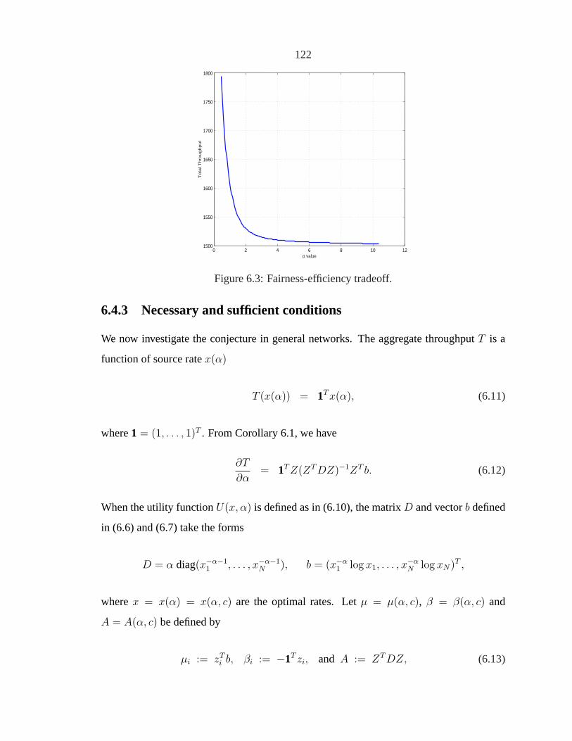
122
0 2 4 6 8 10 121500
1550
1600
1650
1700
1750
1800
α value
Tota
l Thro
ughput
Figure 6.3: Fairness-efficiency tradeoff.
6.4.3 Necessary and sufficient conditions
We now investigate the conjecture in general networks. The aggregate throughputT is a
function of source ratex(α)
T (x(α)) = 1T x(α), (6.11)
where1 = (1, . . . , 1)T . From Corollary 6.1, we have
∂T
∂α= 1T Z(ZT DZ)−1ZT b. (6.12)
When the utility functionU(x, α) is defined as in (6.10), the matrixD and vectorb defined
in (6.6) and (6.7) take the forms
D = α diag(x−α−11 , . . . , x−α−1
N ), b = (x−α1 log x1, . . . , x
−αN log xN)T ,
wherex = x(α) = x(α, c) are the optimal rates. Letµ = µ(α, c), β = β(α, c) and
A = A(α, c) be defined by
µi := zTi b, βi := −1T zi, and A := ZT DZ, (6.13)

123
wherezi are theith columns ofZ. Note thatA is positive definite and hence invertible.
Let Ai(α, c) denote the matrix obtained from replacing theith row of A with row vector
βT = (β1, β2 . . . βM). From the above definitions and (6.12) we have
∂T
∂α= −βT A−1µ. (6.14)
Our first main result is a necessary and sufficient condition for the conjecture to hold.
Note that the condition is a function ofα even though this is not explicit in the notation.
Theorem 6.2.For anyα > 0
∂T
∂α≤ 0 if and only if
M∑i=1
µi det Ai ≥ 0.
Proof: The key observation is the following expression for the row vector
βT A−1 =1
det A
(det A1, det A2, . . . , det An
), (6.15)
which follows from the following formula for matrix inverse [62]
A−1 =1
det AA∗,
whereA∗ is the adjoint matrix ofA. Combining (6.14) and (6.15), we have
∂T
∂α= − 1
det A
M∑i=1
µi det Ai.
Theorem 6.2 characterizes exactly the set of networks(R, c) in which Conjecture 6.1
is true. Though difficult to understand intuitively, this characterization leads directly to
two sufficient conditions that explain all the examples in Section 6.4.2. The first condition
implies that the conjecture is true when every link has a single-link flow and there is only
one long flow. This condition is satisfied by Examples 1 and 2. The second condition

124
implies that the conjecture is true when there are two long flows but both pass through the
same number of links. This condition is satisfied by Example 3. The corollary implies that,
while the diversity of capacitiescl in Examples 2 and 3 makes the optimization problem
(6.2) hard to solve and the previous analysis methods complicated, they are not relevant at
all to the truth of the conjecture for these examples.
Corollary 6.2. Suppose every link has a single-link flow.
1. If dim(Z) = 1, then∂T/∂α ≤ 0 for all α > 0.
2. If dim(Z) = 2 and the only two long flows pass through the same number of links,
then∂T/∂α ≤ 0 for all α > 0.
To prove the corollary, we now specialize to a particular basisZ of the null space of the
routing matrixR, making use of the fact that every link has a single-link flow. Rearrange
the column of routing matrixR to expressR as
R =[
IL R1
],
whereIL is theL× L identity matrix andR1 is aL×M matrix,N = L + M . We choose
a set of basis for the null space ofR such that matrixZ can be expressed as
Z =
−R1
IM
.
Clearly rank(Z) = dim(Z) = M .
Lemma 6.2. Suppose every link has a single-link flow. ForZ in the form of (6.16), we have
1. µm ≥ 0 for m = 1, . . . ,M .
2. amm ≥ amn for all m,n = 1, . . . , M .
Proof: The proof is a series calculations based on the Karush-Kuhn-Tucker conditions.
See [144, 146] for the detailed proof.

125
We are now ready to prove Corollary 6.2 with the above lemma.
Proof of Corollary 6.2: 1) In this case,M = 1 and Z ∈ <N×1 is a column vector.
There areL single-link flows, one at each of theL links, and exactly one other flow that
can traverse one or more links. This means∑L
j=1−z1j ≥ 1 since the long flow at least
transverses one link. Hence
β1 = −1T z1 =L∑
j=1
−z1j − 1 ≥ 0.
From Lemma 6.2, we know thatµ1 > 0. From Theorem 6.2 we have
∂T
∂α= − µ1β1
det A≤ 0
since matrix A is positive definite.
2) In addition to theL single-link flows, there are two flows that traverse one or more
links. Since they traverse the same number of links, we have
β1 = β2 = −1T z1 ≥ 0, (6.16)
as in the first assertion. We also have
µ1 det A1 + µ2 det A2 = β1 [µ1(a22 − a21) + µ2(a11 − a12)] .
Lemma 6.2 and (6.16) then imply that the above quantity is nonnegative. Hence,
∂T
∂α= −µ1 det A1 + µ2 det A2
det A≤ 0.

126
6.4.4 Counter-example
The condition in the second part of Corollary 6.2 that both long flows pass through the
same number of links is important. When it fails, there are networks where theoppositeof
the conjecture is true!
Theorem 6.3.Whendim(Z) ≥ 2, for anyα0 > 0, there exists a network such that
∂T
∂α> 0 for all α > α0
Proof: See the detailed proof in [144, 146] .
Since in reality there are many more flows than bottleneck links and therefore dim(Z)
is typically large, it is conceivable that Conjecture 6.1 is wrong more often than right in
practice.
Example 4: Counter-example
Consider the linear network withL = 5 links andN = 7 sources, shown in Figure 6.4. The
1x
6x
2x 3x 4x 5x
7x
Sc Sc Lc Lc Lc
Figure 6.4: Network for counter-example in Theorem 6.3.
null space ofR has a dimension dim(Z) = N − L = 2. There are five one-link flows with
ratesx1, . . . , x5 and two long flows with ratesx6, x7. Links 1 and 2 have a small capacity
cS, and links 3, 4, and 5 have a large capacitycL. We solve the utility maximization (6.5)
numerically to computeT (α) for α ∈ [0.5, 10].
The aggregate throughputT (α) is plotted in Figure 6.5 as a function ofα, for cS = 10
and cL = 1, 000. The minimal throughput is achieved aroundα0 = 0.95 and will be

127
achieved aroundα0 = 0.75 if we changecL to be5, 000. T (α) is strictly increasing beyond
α0. In particular,
T (∞) > T (2) > T (1).
The example is surprising at first because the conventional wisdom in networking is that
0 2 4 6 8 10 123006.2
3006.4
3006.6
3006.8
3007
3007.2
3007.4
3007.6
3007.8
α value
To
tal T
hro
ug
hp
ut
Figure 6.5: Throughput versus efficiencyα in the counter-example.
increasingα favors long flows that take up more resources, leading to a drop in aggregate
throughput. This is not exactly right. Recall that the pricepl at a link is a precise measure
of congestion at that link. A more precise intuition is that increasingα favors “expensive”
flows, flows that have the largest sum of link prices in their paths. In Example 4, the link
capacitycS is small andcL is large, so that prices are high at links 1 and 2, and low at links
3, 4, and 5. Even thoughx6 traverses more links, it has a lower aggregate price over its
path thanx7. Hence, whenα increases,x7 increases, leading to a reduction inx6 (because
of sharing at link 2). This reduction allows increases in flowsx3, x4,andx5 , so that the net
change in aggregate throughputT (α) is positive. Hence the counter-example relies on the
design that the longest flow is not the most expensive.
Indeed, one can prove that for the network in Figure 6.4,∂x7/∂α > 0 and∂x6/∂α < 0

128
for all α > α0, as illustrated in Figure 6.6. In this example, the decrease inx6 allows
0 2 4 6 8 10 121.5
2
2.5
3
3.5
4
α value
so
urc
e r
ate
x6
x7
Figure 6.6: Source rates versusα in the counter-example.
increases in just three one-link flows, and yet this is enough to produce a net increase in the
aggregate throughput. Our example actually is compact in that our proof shows thatx6 has
to pass through at least three links (link 3,4,5) to make∂T/∂α > 0.
One may notice that the amount of increment in Figure 6.5 is quite small. In fact, an
easy and loose upper-bound for the increment of aggregate throughput iscS/2. Currently,
we don’t know whether this small variation is true only for this example or for general
networks (R, c).
6.5 Does increasing capacity always raise throughput?
We have seen how fairness, as measured byα, can affect efficiency, as measured byT , in
unexpected ways due to interaction among sources in general networks. In this section, we
study how increasing capacityc affects the aggregate throughputT . The results here can
be useful in deciding in which links resources should be invested to maximize aggregate
throughput.
Let δ ∈ RL be the vector that represents the increases in link capacities in the entire
129
network. For instance, whenδ = εel, whereε > 0 is a small scalar, andel is aL-vector that
has all its entries 0 except thel-th entry which is 1, then only linkl increases its capacity
from cl to cl + ε. Whenδ = ε1, then all links increase their capacities byε unit. When
δ = εc, then all links increase their capacities by amounts proportional to their current
capacities.
The change in aggregate throughput per unit of an infinitesimal changeδ in capacities
is measured by the directional derivativeDT of T in directionδ, defined as
DT (α, δ) = DT (α, δ; c) := limε→0
T (α, c)− T (α, c + εδ)
ε.
From (6.11), we have
DT (α, δ) = 1T ∂x
∂cδ,
where∂x/∂c is evaluated at the optimal ratex(α, c). We will takeδ to denote thedirec-
tion of increase in capacity, with the understanding thatε DT (α, δ) provides an estimate of
change in aggregate throughput whenc is changed toc + εδ. Our results should be inter-
preted in the context of small perturbations that do not change the active constraint set in
(6.2).
DefineB = RD−1RT , η = 1T D−1RT , andBi is the matrix obtained by replacingith
row of B by η. A similar argument to the proof of Theorem 6.2 yields the following:
Theorem 6.4.For anyδ, α > 0
DT (α, δ) ≥ 0 if and only ifL∑
i=1
δi det Bi ≥ 0.
Theorem 6.4 characterizes exactly the set of all networks(R, c), and directionsδ, in
which aggregate throughput will increase, forall fairnessα > 0. An easy consequence is
the following:
Corollary 6.3. If R has only two rows, thenDT (α, δ) ≥ 0 for anyα > 0 and anyδ ≥ 0.
Proof: Let Bij denote the(i, j) element ofB. A similar argument to the proof of Lemma

130
6.2 shows that
ηi = Bii, and Bii ≥ Bij = Bji for i, j = 1, 2.
Then
det(B1) = η1B22 − η2B21 = b22(B11 −B21) ≥ 0.
Similarly we havedet(B2) ≥ 0. From Theorem 6.4, we haveDT (α, δ) ≥ 0.
Corollary 6.3 says that increasing link capacity always raises aggregate throughput,
provided there are only two bottleneck links. Intuitively, one might expect this to hold
more generally. This is however not the case. We provide three interesting examples, with
different instantiations of directionδ, as an illustration.
The first result says that not only can the aggregate throughput be reduced when some
link increases its capacity; paradoxically, it can also be reduced whenall links increase
their capacities by the same amount. This is true for almost all fairnessα.
Theorem 6.5.Given anyα0 > 0,
1. there exists a network (R, c) such that for allα > α0, DT (α, el) < 0 for some linkl.
2. there exists a network (R, c) such that for allα > α0, DT (α, 1) < 0.
Proof: The proof is by construction. For the first claim, consider the network in Figure 6.7.
c5
c1
c2
c3
c4
Figure 6.7: Counter-example for Theorem 6.5(1).
There is a single-link flowxl at each linkl, for l = 1, . . . 4. The flowx5 transverses links

131
1, 2, and5, and flowx6 transverses links3, 4, and5 respectively. The capacities of the links
arec1 = c2 = c3 = c4 = cL andc5 = cS. We increase only link 5’s capacity by 1, which
corresponds toδ = e5. For any fixedα0 > 0, we can choosecL/cS large enough, such that
for anyα > α0 all links are fully utilized. Calculating the change in aggregate throughput
using Mathematica gives
DT (α, e5) = 1T ∂x
∂ce5 = 1T D−1RT
(RD−1RT
)−1e5 = −1.
For the second claim, consider the network shown in Figure 6.8. There is a single-link
c2
c1
c3
c4 c5 c10
x13
x11
x12
Figure 6.8: Counter-example for Theorem 6.5(2).
flow xl at each linkl, for l = 1, ..., 10. The link capacities arecl = cS for l = 1, 2, 3 and
cl = cL for l = 4, . . . , 10. We skip the detailed proof ofDT (α, 1) < 0, which can be found
in [144, 146].
Example 5: DT (∞, 1) < 0 for somec in Figure 6.8
To illustrate, we calculate the change in aggregate throughput for the network in Figure 6.8
under max–min policyα = ∞. Let the link capacities becS = 2 andcL = 10. The source
can be easily calculated under max-min fairness, and it is easy to check that the aggregate
throughput is55. When all capacities are increased by2ε with 0 ≤ ε ≤ 1, we can check
that the total throughputT (ε) changes into55 − ε, i.e.,T (ε) is a decreasing function ofε.
IndeedDT (∞, 1) = −1/2 < 0 in this situation.

132
If link capacities are increased proportionally, i.e., ifc is increased to(1 + ε)c, then
aggregate throughput will always rise. Note that even though increasing all link capacities
proportionally may be interpreted as changing the unit of capacity, it doesnot imply that
general utility functions increase proportionally in optimal flow vectors. It does however
imply this for the class of utility functions defined in (6.10).
Theorem 6.6.For any network (R,c) and for allα > 0, DT (α, c) > 0.
Proof: The necessary and sufficient condition for anyx ≥ 0 andp ≥ 0 to be primal and
dual optimal are
Rx = c, and RT p =∂V
∂x= (x−α
1 , . . . , x−αN )T .
Supposex andp are optimal with link capacitiesc. Whenc is increased to(1 + ε)c for
ε > 0, we claim thatx(1 + ε) and(1 + ε)−αp are the new optimal rate and price vectors,
respectively. We can check that these vectors satisfy the optimality condition for capacity
(1 + ε)c
Rx(1 + ε) = c(1 + ε),
RT p(1 + ε)−α = (1 + ε)−α(x−α1 , . . . , x−α
N )T =∂V
∂x.
Therefore, the aggregate throughput is increased from the original valueT to (1 + ε)T .
Hence, we haveDT (α, c) = T > 0.
6.6 Conclusion
A bandwidth allocation policy can be defined in terms of utility functions parameterized
by some protocol parameterα. We have studied how throughputs and prices change as
link capacities orα changes. We then focus on a specific class of utility functions where
α can be interpreted as a quantitative measure of fairness. We say an allocation is fair ifα
is large and efficient if the aggregate throughput is large. We use this model to investigate
whether a fairer allocation is always more inefficient and whether increasing link capacities

133
always raises throughput. We characterize exactly the set of all networks(R, c) in which
the answers are “yes.” Though these characterizations are difficult to understand intuitively,
they have led to simple corollaries that explain all the examples we found in the literature
and to the discovery of the first counter examples.
There are a number of ways this preliminary work can be extended. First, we have
focused of how throughputsx change in response to changes inα andc, which is only half
of Theorem 6.1. The application of the other half of Theorem 6.1 on how prices change
has not been exploited. Second, the necessary and sufficient conditions for the conjectures
are hard to understand intuitively and check for large networks. It is not clear whether
this condition is likely to hold or fail in practice. It would be useful to derive equivalent
characterizations that are more intuitive or more general corollaries than reported here.
Finally, we have assumed that every source has the same utility function. It would be
interesting to see how the fairness definition and tradeoff results should generalize when
sources have the same class of utility functions but with differentαi parameters, or have
different utility functions.
134
Chapter 7
Other Related Projects
7.1 Network equilibrium with heterogeneous protocols
7.1.1 Introduction
As we have seen in the previous chapters, congestion control protocols can be modelled
as distributed algorithms to maximize the aggregate utility, e.g., [80, 97, 116, 164, 88,
96]. However, these studies assume that all sources are homogeneous, that is, even though
they may control their rates using different algorithms, they all adapt to the same type of
congestion signals, e.g., loss probabilities in TCP Reno and queueing delay in FAST TCP
[69]. When sources withheterogeneousprotocols that react to different congestion signals
share the same network, the current duality framework is no longer applicable. With new
congestion control algorithms proposed for large bandwidth-delay product networks and
usage of congestion signals other than packet losses (including explicit feedbacks with
ECN), we need a rigorous framework to understand the behavior of large-scale networks
with heterogeneous protocols.
A congestion control protocol generally takes the form
pl = gl
∑
j:l∈L(j)
xj(t), pl(t)
, xj = fj
xj(t),
∑
l∈L(j)
mjl (pl(t))
. (7.1)
As we have shown in Chapter 2, heregl(·) models a queue management algorithm, and
fj(·) models a TCP algorithm. The effective pricesmjl (pl(t)) are functions of the link

135
pricespl(t), which in general can vary depending on the links and source.
When all algorithms use the same pricing signal (i.e., homogeneous protocols with
mjl = ml for all j), the equilibrium of (7.1) turns out to be very simple. At the equilibrium,
the source ratesxi solve a utility maximization problem, and the link congestion measure
pl serves as a Lagrange dual. When heterogeneous algorithms that use different pricing
signals share the same network, i.e.,mjl are different for different sourcesj, the situation
is much more complicated. For instance, when TCP Reno and FAST TCP share the same
network, neither loss probability nor queueing delay can serve as the Lagrange multiplier at
the link, and (7.1) can no longer be interpreted as solving the standard utility maximization
problem. Basic questions, such as the existence and uniqueness of equilibrium, and its
local and global stability, need to be re-examined.
7.1.2 Model
A network consists of a set ofL links with finite capacitiescl. There areJ different proto-
cols indexed by superscriptj, and there areN j sources using protocolj indexed by(j, i).
The total number of sources isN :=∑
j N j. The L × N j routing matrixRj for type
j sources is defined byRjli = 1 if source(j, i) uses linkl, and 0 otherwise. The overall
routing matrix is denoted byR =[
R1 R2 · · · RJ
].
Every link l has a pricepl. A type j source reacts to the “effective price”mjl (pl) in
its path. By specifying functionmjl , we can let the link feed back different congestion
signals to sources using different protocols. The end-to-end prices for source(j, i) is qji =
∑l R
jlim
jl (pl). Let qj = (qj
i , i = 1, . . . , N j), q = (qj, j = 1 . . . , J), mj(p) = (mjl (pl), l =
1, . . . L) andm(p) = (mj(pl), j = 1, . . . J) be vector forms. Thenqj = (Rj)T
mj(p) and
q = RT m(p).
Let xj be a vector with the ratexji of source(j, i) as itsith entry, and letx be the vector
of xj. We suppose that source(j, i) has a utility functionU ji (xj
i ) that is strictly concave
and increasing.
A network is in equilibrium when each source(j, i) maximizes its net benefit and the
demand for and supply of bandwidth at each bottleneck link are balanced. Formally, a

136
network equilibrium is defined as follows.
Given pricesp, the end-to-end price vectorq is formulated asq = RT m(p). The
source ratexji is uniquely determined byqj
i , and it uniquely solvesmaxz≥0 U ji (z) − zqj
i .
Therefore, the source rates vectorx is a function of link pricesp, denoted asx(p). Denote
y(p) as the aggregate source rates at links, theny(p) = Rx(p).
In equilibrium, the aggregate rate at each link is no more than the link capacity, and
they are equal if the link price is strictly positive. Formally, we callp anequilibrium if it
satisfies
P (y(p)− c) = 0, y(p) ≤ c, p ≥ 0 (7.2)
whereP := diag(pl) is a diagonal matrix. We will study the existence and uniqueness
properties of network equilibrium specified by the above equations.
7.1.3 Existence of equilibrium
We prove the existence of equilibrium under the following assumptions.
A1: Utility functions U ji are strictly concave, increasing, and twice differentiable. Price
mapping functionsmjl are differentiable and strictly increasing withmj
l (0) = 0.
A2: For anyε > 0, there exists a numberpmax such that ifpl > pmax for link l, then
xji (p) < ε for all (j, i) with Rj
li = 1.
These assumptions are mild. Concavity and monotonicity of utility functions are often
assumed in network pricing for elastic traffic. The assumption onmjl preserves the relative
order of prices and maps zero price to zero effective price. Assumption A2 says that when
pl is high enough, then every source going through linkl has a rate less thanε.
Theorem 7.1. Suppose A1 and A2 hold. There exists an equilibrium pricep∗ for any
network(c,m, R, U).
The mathematical tool used to prove this theorem is the Nash theorem in game theory
[121, 10], which is an application of Kakutani’s generalized fixed point theorem. The
detailed proof can be found in [147].

137
7.1.4 Examples of multiple equilibria
Theorem 7.1 guarantees the existence of network equilibrium; however the equilibrium
may not be unique. We show two examples of multiple equilibria.
In a single-protocol network, if the routing matrix R has full row rank, then there is
a unique active constraint set. In contrast, the active constraint set in a multi-protocol
network can be non-unique even if R has full row rank as shown in Example 1. Clearly, the
equilibrium prices associated with different active constraint sets are different.
Example 1: Multiple equilibria with different active constraint sets
Consider a symmetric network in Figure 7.1 with three flows. The link 1 and link 3 have
1x12x1
1x2
Figure 7.1: Example 2: two active constraint sets.
identical parameters, and flows(1, 1) and(1, 2) have identical utility function. We show
that [142], under certain conditions, the network has two equilibria with different congested
links. We also carry out experiments with TCP Reno, which reacts to loss probability,
and TCP Vegas/FAST, which reacts to delay, and we set the experiment parameters such
that the conditions are satisfied. The prices (queues) at link 1 and link 2 are shown in
Figure 7.2. This result unambiguously exhibits that there are two equilibria with different
active constraint sets. The queue flip is produced when the network operates at different
equilibria.
Example 2: Multiple equilibria with a unique active constraint set
When the active constraint set is unique, it is still possible to have multiple equilibria,
and even uncountable many of them. We show that such an example withJ = 3. The

138
0 100 200 300 400 500 600 700 800 900 10000
100
200
300
400
Simulation time (sec)
Lin
k1
Qu
eu
e S
ize
(p
kts
)
0 100 200 300 400 500 600 700 800 900 10000
50
100
150
200
250
300
Simulation time (sec)
Lin
k2
Qu
eu
e S
ize
(p
kts
)
Figure 7.2: Shifts between the two equilibria with different active constraint sets.
network is shown in Figure 7.3 with three unit-capacity links,cl = 1. All the sources use
1x12x1
1x2
1x3
3x1
2x2
Figure 7.3: Example 2: uncountably many equilibria.
the same utility functionU ji (xj
i ) = − (1− xj
i
)2/2, and the price mapping function is linear
mj(p) = Kjp, whereKj areL × L diagonal matrices withK1 = I, K2 = diag(5, 1, 5),
andK3 = diag(1, 3, 1).
It can be shown that the equilibrium pricep satisfies
∑j
Rj(Rj)T Kjp =∑
j
Rj1− c
which is a linear equation inp. It has a unique solution if the determinantdet(∑
j Rj(Rj)T Kj)

139
is nonzero, but has no or multiple solutions otherwise. By choosing appropriate parameters
(as shown above), we can make this determinant zero. It is easy to check that all of the
following are equilibrium prices for this network
p11 = p1
3 = 1/8 + ε, and p12 = 1/4− 2ε where ε ∈ [0, 1/24].
The corresponding source rates can also be derived, and all capacity constraints are tight
with these rates, yet there are uncountably many equilibria.
Examples 1 and 2 show that global uniqueness is generally not guaranteed in a multi-
protocol network. We will show, however, that local uniqueness is basically a generic
property of the equilibrium set.
7.1.5 Local uniqueness of equilibrium
We denoteE as the equilibrium set wherep is in E if and only if it satisfies (7.2). Fix an
equilibrium pricep∗ ∈ E. Let theactive constraint setL = L(p∗) ⊆ L be the set of links
at whichp∗l > 0. Consider the reduced system that consists only of links inL, and denote
all variables in the reduced system byc, p, y, etc. Then, sinceyl(p) = cl for everyl ∈ L,
we havey(p) = c. Let the Jacobian for the reduced system beJ(p) = ∂y(p)/∂p, and
J(p) =∑
j
Rj ∂xj(p)
∂qj
(Rj
)T ∂mj(p)
∂p. (7.3)
Since the equilibrium pricep∗ for the links inL is a solution ofy(p) = c, by the inverse
function theorem, the equilibrium pricep∗, is locally uniqueif the Jacobian matrixJ(p∗) =
∂y/∂p is nonsingular atp∗. We call a networkregular if all its equilibrium prices are locally
unique. The following theorem shows that almost all networks are regular and that regular
networks have finitely many equilibrium prices. This implies that the uncountablly many
equilibria shown in Example2 almost never happens in real networks.
Theorem 7.2. Suppose assumptions A1 and A2 hold. Given any price mapping functions
m, any routing matrixR and utility functionsU ,

140
1. the set of link capacitiesc for which not all equilibrium prices are locally unique has
Lebesgue measure zero in<L+.
2. the number of equilibria for a regular network(c, m,R, U) is finite.
We now narrow our attention to networks that satisfy an additional assumption:
A3: Every link l has a single-link flow.(j, i) with(U j
i
)′(cl) > 0.
Assumption A3 says that when the price of linkl is small enough, the aggregate rate
through it will exceed its capacity. It implies that the active constraint set is unique and
contains every link.
Since all the equilibria of a regular network have nonsingular Jacobian matrices, we
can define theindexI(p) of p ∈ E as
I(p) =
1 if det (J(p)) > 0
−1 if det (J(p)) < 0.
Theorem 7.3.Suppose assumptions A1–A3 hold. Given any regular network, we have
∑p∈E
I(p) = (−1)L
whereL is the number of links.
The proof of this theorem is based on the Poincare-Hopf index Theorem [149, 113].
First, we construct a vector field formed by a continuous-time gradient project algorithm
[97] with multiple protocols. Clearly,p∗ is an equilibrium point of this vector field if and
only if it is a network equilibrium. Under the assumption A3, there will be a contraction
region in this vector field, and all the equilibria are in this region. The Jacobian matrix of
the vector field equilibrium point is the same as 7.3 if uniform stepsize is used. Since the
network is regular, every equilibrium has an index. Using the Poincare-Hopf index theorem
gives us the result in Theorem 7.3. An obvious consequence of this theorem is:
Corollary 7.1. Suppose assumptions A1–A3 hold. A regular network has an odd number
of equilibria.

141
Corollary 7.1 also implies the existence of an equilibrium, although we show this in a
more general setting in Section 7.1.3. Next we will present another example to illustrate
Theorem 7.3 and Corollary 7.1.
Example 3: Illustration of Theorem 7.3 and Corollary 7.1
Recall that in Example 1, there are uncountably many equilibria. The componentsx11
andq11 of these equilibrium points are shown by the (red) solid line in Figure 7.4. We can
change the utility function of every source into the following form
U ji (xj
i , αji ) =
βji (x
ji )
1−αji /(1− αj
i ) if αji 6= 1
βji log xj
i if αji = 1
,
whereαji andβj
i are parameters. We pick two points (the two black dots), and choose ap-
propriate parametersαji andβj
i for every source, such that these two points will be isolated
equilibria.
After this perturbation, we can check whether the two designed equilibria are locally
unique, and the network is regular. Corollary 7.1 predicts an odd number of equilibria. We
indeed can find another equilibrium, and three of them in total 7.4.
x 11
q 11
1=(β11/q
11)1/α1
1 x 1
5/6
7/8
1/8 1/6
(0.135,0.865)
(0.165,0.835)
Figure 7.4: Example 3: construction of multiple isolated equilibria.
We further check the local stability of these three equilibria under the gradient algo-
rithm. It turns out that one of them is not stable and has index 1, while the other two are

142
stable with index−1. The dynamics of this network under the gradient algorithm can be
illustrated by a vector field. We draw the vector field restricted on the planep1 = p3, and
the phase portrait is shown in Figure 7.5. The (red) dots represent the three equilibria. Note
that the equilibrium in the middle is a saddle point, and it is therefore unstable. The (red)
arrows give the direction of this vector field. Individual trajectories are plotted with slim
(blue) lines.
0.1 0.11 0.12 0.13 0.14 0.15 0.16 0.17 0.18 0.19 0.20.15
0.16
0.17
0.18
0.19
0.2
0.21
0.22
0.23
0.24
0.25
p1
p 2
Figure 7.5: Example 3: vector field of (p1, p2).
7.1.6 Global uniqueness of equilibrium
The exact condition under which network equilibrium is globally unique is generally hard
to prove. We provide several special cases for global uniqueness.
Theorem 7.4. Suppose assumptions A1–A3 hold. If all equilibria have index(−1)L, then
E contains exactly one point. In particular, if all equilibria are locally stable, thenE
contains exactly one point.
The first claim of the theorem directly follows from Theorem 7.3. It can be checked
that a local stable equilibrium also has an index of(−1)L, and the second claim also holds.
This result relates the local stability of an algorithm to the uniqueness property of a
network. Local stability can be checked in several ways, and it can be used to prove global
uniqueness. We will concentrate on several special cases in the rest of this section.

143
Theorem 7.5. Suppose assumptions A1–A3 hold andR has full row rank. If for allj and
l, mjl (pl) = kjpl for some scalarkj > 0, then there is a unique network equilibrium .
Under the assumption of Theorem 7.5, it is easy to show that we have an unusual situ-
ation in the theory of heterogeneous protocols where the equilibrium rate vectorx solves
the following concave maximization problem
maxx
∑i,j
kjU ji (xj
i ) s. t.Rx ≤ c.
Therefore, such a network always has a globally unique equilibrium whenU ji are strictly
concave. It can also be proved using Theorem 7.4 by showing that every equilibrium is
locally stable under the gradient projection algorithm.
Theorem 7.6. Suppose assumptions A1–A2 hold. The linear network in Figure 7.6 has a
unique equilibrium.
7.6. We can show that every equilibrium in this network is locally stable and that even
1x
L+1x
2x LxFigure 7.6: Corollary 7.6: linear network.
every source uses different protocols. By Theorem 7.4, the equilibrium is globally unique.
Theorem 7.4 also implies the global uniqueness of equilibrium for any network in which
no flow passes through more than 2 links in the active constraint set, when A1–A3 hold. In
this case, the Jacobian matrix is strictly diagonally dominant with negative diagonal entries,
and hence its determinant is(−1)L.
Theorem 7.7.Suppose assumptions A1–A3 hold. A network where all flows using at most
two links has a unique equilibrium.

144
7.1.7 Conclusion
When sources sharing the same network react to different pricing signals, the current dual-
ity model no longer explains the equilibrium of bandwidth allocation. We have introduced a
mathematical formulation of network equilibrium for multi-protocol networks and studied
several fundamental properties, such as existence, local uniqueness, number of equilibria,
and global uniqueness. We prove that equilibria exist and are almost always locally unique.
The number of equilibria is almost always finite and must be odd when they are associ-
ated with the same active constraint set. We provide four sufficient conditions for global
uniqueness.
The utility maximization problem that underlies a single-protocol network implies that
the equilibrium source rates exist and are always unique [96]. In the heterogeneous protocol
case, we prove that equilibrium still exists, under mild conditions, despite the lack of an un-
derlying concave optimization problem. There can be uncountably many equilibria, and the
bottleneck links set can be also be non-unique. However, we prove that almost all networks
have finitely many equilibria and that they are necessarily locally unique. Non-uniqueness
can arise in two ways. First, the equilibria associated with different sets of bottleneck links
are always distinct. Second, the number of equilibria associated with each set of bottleneck
links can be more than one, though always odd. Moreover, these equilibria cannot all be
locally stable unless the equilibrium is globally unique. We also provide several special
cases for global uniqueness of network equilibrium. We also provide numerical examples
to illustrate the theorem and equilibrium properties.
7.2 Control unresponsive flow–CHOKe
7.2.1 Introduction
TCP is believed to be largely responsible for preventing congestion collapse while the In-
ternet has undergone dramatic growth in the last decade. Indeed, numerous measurements
have consistently shown that more than 90% of traffic on the current Internet still consists
of TCP packets, which, fortunately, are congestion controlled. Without a proper incen-

145
tive structure, however, this state of affairs is fragile and can be disrupted by the growing
number of non-rate-adaptive (e.g., UDP-based) applications that can monopolize network
bandwidth to the detriment of rate-adaptive applications. This has motivated several active
queue management schemes, e.g., [111, 41, 94, 141, 123, 126, 35], that aim at penalizing
aggressive flows and ensuring fairness. The scheme, CHOKe, of [126] is particularly in-
teresting in that it does not require any state information and yet can provide a minimum
throughput to TCP flows.
The basic idea of CHOKe is explained in the following quotation from [126]:
“When a packet arrives at a congested router, CHOKe draws a packet at random from
the FIFO (first-in-first-out) buffer and compares it with the arriving packet. If they both
belong to the same flow, then they are both dropped; else the randomly chosen packet
is left intact and the arriving packet is admitted into the buffer with a probability that
depends on the level of congestion (this probability is computed exactly as in RED). ”
The surprising feature of this simple scheme is that it can bound the bandwidth share of
UDP flows regardless of their arrival rate. Extensive simulation results in [126] show that
as the arrival rate of UDP packets increases without bound, their bandwidth share peaks and
then drops to zero! It seems intriguing that a flow that maintains a much larger number of
packets in the queue does not receive a larger share of bandwidth, as in the case of a regular
FIFO buffer. We provide an analytical model of CHOKe that explains both this throughput
behavior and the spatial characteristics of its leaky buffer. In this section, we will present
the model, analysis, and simulations of CHOKe very briefly. See [155, 143, 145] for details.
7.2.2 Model
We focus on a network with a single bottleneck link with capacityc pkts/sec, which is
shared by byN identical TCP sources and a UDP flow with a constant sending rate. We
study the network’s equilibrium behavior.
Equilibrium quantities (rate, dropping probability, etc.) associated with the UDP flow
are indexed by 0. Since the TCP sources are identical, we will use index 1 for all TCP

146
flows. The definition of all variables and some of their obvious properties are collected
below:
d: common round-trip propagation delay for TCP sources.
τ : common queueing delay, and round-trip delay isd + τ .
bi: packet backlog from flowi, i = 0, 1.
b: total backlog;b = b0 + b1N .
r: congestion based dropping probability. In general,r = g(b, τ) whereg is a function
of aggregate backlogb and queueing delayτ .
xi: source rate of flowi. In general,x1 = f(p1, τ) wheref is a function of overall loss
probabilityp1 and queueing delayτ .
hi: the probability that an incoming packet of flowi is dropped by CHOKehi = bi/b.
pi: overall probability that a packet of flowi is dropped before it gets through.
A packet may be dropped, either on arrival due to CHOKe or congestion (e.g., according
to RED) or after it has been admitted into the queue when a future arrival from the same
flow triggers a comparison. Every arrival packet from flowi can trigger either0 packet loss
from the buffer, 1 packet loss due to RED, or 2 packet losses due to CHOKe. These events
happen with respective probabilities of(1 − hi)(1 − r), (1 − hi)r, andhi. Hence, each
arrival to the buffer is accompanied by an average packet loss of
pi = 2hi + (1− hi)r + 0 · (1− hi)(1− r) = 2hi + r − rhi. (7.4)
Consider a packet of flowi that eventually goes through the queue without being dropped.
The probability that it is not dropped on arrival is(1− r)(1−hi). Once it enters the queue,
it takesτ time to go through it. In this time period, there are on averageτxi packets from
flow i that arrive at the queue. The probability that this packet is not chosen for comparison
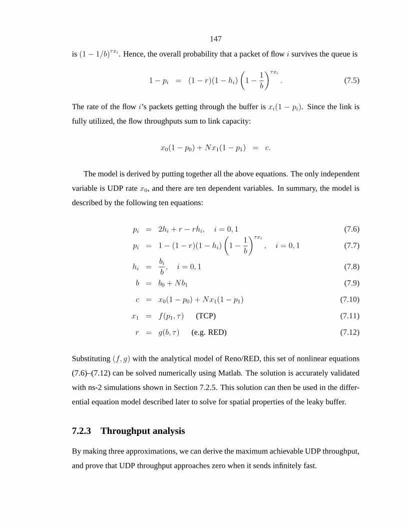
147
is (1− 1/b)τxi. Hence, the overall probability that a packet of flowi survives the queue is
1− pi = (1− r)(1− hi)
(1− 1
b
)τxi
. (7.5)
The rate of the flowi’s packets getting through the buffer isxi(1 − pi). Since the link is
fully utilized, the flow throughputs sum to link capacity:
x0(1− p0) + Nx1(1− p1) = c.
The model is derived by putting together all the above equations. The only independent
variable is UDP ratex0, and there are ten dependent variables. In summary, the model is
described by the following ten equations:
pi = 2hi + r − rhi, i = 0, 1 (7.6)
pi = 1− (1− r)(1− hi)
(1− 1
b
)τxi
, i = 0, 1 (7.7)
hi =bi
b, i = 0, 1 (7.8)
b = b0 + Nb1 (7.9)
c = x0(1− p0) + Nx1(1− p1) (7.10)
x1 = f(p1, τ) (TCP) (7.11)
r = g(b, τ) (e.g. RED) (7.12)
Substituting(f, g) with the analytical model of Reno/RED, this set of nonlinear equations
(7.6)–(7.12) can be solved numerically using Matlab. The solution is accurately validated
with ns-2 simulations shown in Section 7.2.5. This solution can then be used in the differ-
ential equation model described later to solve for spatial properties of the leaky buffer.
7.2.3 Throughput analysis
By making three approximations, we can derive the maximum achievable UDP throughput,
and prove that UDP throughput approaches zero when it sends infinitely fast.

148
First, we approximate the system by one in which the order of congestion based drop-
ping and CHOKe is reversed. Second, we assume thatN is large such that a comparison
triggered by aTCParriving packet never yields a match. The last assumption is that we can
approximate(1− 1/b)b ' e−1. Under these assumptions, we can eliminateτ in the model
(7.6)–(7.12) and get our key equation
1− h0
1− 2h0
= exp
(x0(1− r)(1− h0)
c− x0(1− r)(1− 2h0)
). (7.13)
Let µ0 = µ0(x0) denote the UDP throughput share,µ0 = x0(1 − p0)/c, and let
µ∗0 = maxx0≥0 µ0(x0) denote the maximum achievable UDP share. The UDP through-
put behavior can be totally captured using equation (7.13), which is independent of TCP
and AQM algorithms. We show the bandwidth properties in Theorem 7.8 and visualize it
in Figure 7.7 which shows UDP throughput versus sending rates.
100
101
0
0.05
0.1
0.15
0.2
0.25
0.3
0.35
0.4
0.45
0.5
µ0 U
DP
bandw
idth
share
x0(1-r)/c
Peak Value 0.269
Figure 7.7: Bandwidth shareµ0 v.s. Sending ratex0(1− r)/c.
Theorem 7.8.The UDP throughput has the following properties:
1. The maximum UDP bandwidth share isµ∗0 = (e + 1)−1 = 0.269. It is attained
when the UDP input rate after congestion based dropping isx∗0(1 − r∗) = c(2e −1)/(e + 1) = 1.193c. In this case, the CHOKe dropping rate for UDP ish∗0 =
(e− 1)/(2e− 1) = 0.387.

149
2. As the UDP sending rate grows without bound, even though UDP packets occupy up
to half of the queue, its throughput drops to zero. That is, asx0 →∞, b0 → b/2 but
µ0 → 0.
The second result of the theorem can also be proved without using the three approxi-
mations. See proofs and more details in [155, 143, 145].
7.2.4 Spatial characteristics
We now derive the spatial characteristics of the leaky buffer under CHOKe that give rise to
the macroscopic properties of maximum and asymptotic throughput proved in the previous
subsection.
Lety ∈ [0, b] denote a position in the queue, withy = 0 being the tail. Definev(y) as the
velocity at which the packet at positiony moves toward the head of the queuev(y) = dy/dt.
For instance, the velocity at the head of the queue equals the link capacity,v(b) = c. Let
ρi(y) be the probability that the packet at positiony belongs to flowi, i = 0, 1. The
bandwidth shareµi is the probability that the head of the queue is occupied by a packet
from flow i, µi = ρi(b). We can derive an ordinary differential equation (ODE) model of
these two quantities
v′(y) = β (ρ0(y)x0 + (1− ρ0(y))x1) , (7.14)
ρ′0(y) = β(x0 − x1) ρ0(y)(1− ρ0(y))1
v(y), (7.15)
whereβ = log(1− 1/b), and the boundary conditions are
v(b) = c, and ρi(0)v(0) = xi(1− r)(1− hi), i = 0, 1.
The spatial characteristics of the leaky buffer under CHOKe are totally captured by
these differential equations. Now we present some structural properties of the velocity
v(y) and spatial distributionρ0(y), which are shown in Theorems 7.9, 7.10, and illustrated
in Figure 7.8.
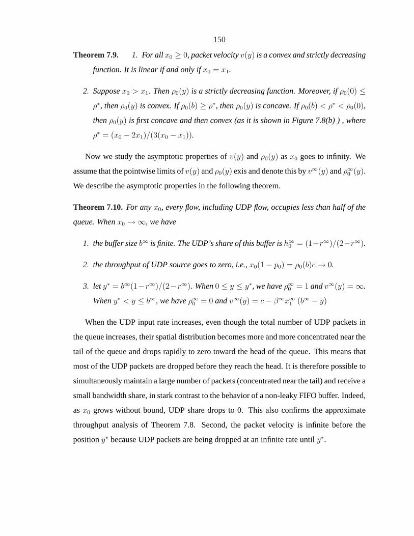
150
Theorem 7.9. 1. For all x0 ≥ 0, packet velocityv(y) is a convex and strictly decreasing
function. It is linear if and only ifx0 = x1.
2. Supposex0 > x1. Thenρ0(y) is a strictly decreasing function. Moreover, ifρ0(0) ≤ρ∗, thenρ0(y) is convex. Ifρ0(b) ≥ ρ∗, thenρ0(y) is concave. Ifρ0(b) < ρ∗ < ρ0(0),
thenρ0(y) is first concave and then convex (as it is shown in Figure 7.8(b) ) , where
ρ∗ = (x0 − 2x1)/(3(x0 − x1)).
Now we study the asymptotic properties ofv(y) andρ0(y) asx0 goes to infinity. We
assume that the pointwise limits ofv(y) andρ0(y) exis and denote this byv∞(y) andρ∞0 (y).
We describe the asymptotic properties in the following theorem.
Theorem 7.10.For anyx0, every flow, including UDP flow, occupies less than half of the
queue. Whenx0 →∞, we have
1. the buffer sizeb∞ is finite. The UDP’s share of this buffer ish∞0 = (1−r∞)/(2−r∞).
2. the throughput of UDP source goes to zero, i.e.,x0(1− p0) = ρ0(b)c → 0.
3. let y∗ = b∞(1−r∞)/(2−r∞). When0 ≤ y ≤ y∗, we haveρ∞0 = 1 andv∞(y) = ∞.
Wheny∗ < y ≤ b∞, we haveρ∞0 = 0 andv∞(y) = c− β∞x∞1 (b∞ − y)
When the UDP input rate increases, even though the total number of UDP packets in
the queue increases, their spatial distribution becomes more and more concentrated near the
tail of the queue and drops rapidly to zero toward the head of the queue. This means that
most of the UDP packets are dropped before they reach the head. It is therefore possible to
simultaneously maintain a large number of packets (concentrated near the tail) and receive a
small bandwidth share, in stark contrast to the behavior of a non-leaky FIFO buffer. Indeed,
asx0 grows without bound, UDP share drops to 0. This also confirms the approximate
throughput analysis of Theorem 7.8. Second, the packet velocity is infinite before the
positiony∗ because UDP packets are being dropped at an infinite rate untily∗.

151
y
v(y)
x0 = x1
c
y
v(y)
x0 = x1
c
y
v(y)
c
10xx ≠
y
v(y)
c
∞=0
x
bb bb bbbr
r
−
−
2
1
(a) Velocityv(y)
y
ρ0(y)
x0 = x1
y
∞=0
x
ybb b
ρ0(y) ρ0(y)
br
r
−
−
2
1
x0 > x1
(b) Spatial distributionρ0(y)
Figure 7.8: Illustration of Theorems 7.9 and 7.10.

152
7.2.5 Simulations
We implement a CHOKe module in ns-2 version 2.1b9. We have conducted extensive
simulations with a single bottleneck link network. This network is shared byN newReno
TCP sources and one UDP source which sends data at a constant rate. We present three
sets of simulation results. The first set illustrates the accuracy of our TCP/CHOKe model
(7.6)–(7.12) and its macroscopic properties. The second set illustrates the spatial properties
proved in Theorem 7.10. The third example uses TCP Vegas and illustrates that these
properties are insensitive to the specific TCP algorithms.
For the newReno simulations in the first two sets the link capacity is fixed at 125
pkts/sec, and round-trip propagation delay is 100ms. We use RED+CHOKe as the queue
management with RED parameters minthb = 20 packets, maxthb = 520 packets,pmax =
0.5. The corresponding analytical model for Reno (functionf ) and RED (functiong) can
be found in Chapter 3.
In our simulation, we vary the UDP sending ratex0 from 0.1c to 10c and measure the
aggregate queue sizeb, UDP bandwidth shareµ0 = ρ0(b), and TCP throughputµ1. We
also solve for these quantities using the analytical model (7.6)–(7.12) and the approximate
model described in Section 7.2.3. The results, shown in Figures 7.9, illustrate both the
macroscopic behavior of TCP/CHOKe and the accuracy of our analytical models.
As can be seen from Figure 7.9, the aggregate queue lengthb steadily increases as
the UDP ratex0 rises. UDP bandwidth shareµ0 = ρ0(b) rises, peaks, and then drops to
less than 5% asx0 increases from0.1c to 10c, while the total TCP throughput follows an
opposite trend, eventually exceeding 95% of the capacity (not shown). These results match
closely those obtained in [126], for both the analytical model and the approximate mode.
Figure 7.9(b) also displays the UDP bandwidth share measured from the simulations for
the casesx0 = 0.1c, c, 10c. It verifies Theorems 7.8 that predicts that the UDP bandwidth
share peaks at around 0.269 and tends to zero asx0 increases.
The next set of results measures the spatial distributionsρ0(y) of UDP packets in the
above simulations shown in Figure 7.9. The simulation results, and analytical solutions, are
both shown in Figure 7.10. They match well Theorem 7.10 and agree with Figure 7.8(b)

153
10−1
100
101
0
20
40
60
80
100
120
140
160
UDP sending rate/capacity, c=125pkts/sec
queue s
ize (
pkts
)
SimulationModelApproximate Model
(a) Queue sizeb
10−1
100
101
0
0.05
0.1
0.15
0.2
0.25
0.3
0.35
0.4
0.45
0.5
UD
P b
an
dw
idth
sh
are
UDP sending rate/capacity, c=125pkts/sec
x0=0.1c
share=0.0777
x0=c
share=0.2474
x0=10c
share=0.0195
SimulationModelApproximate Model
(b) UDP bandwidth shareµ0
Figure 7.9: Experiment 1: effect of UDP ratex0 on queue size and UDP share
in Section 7.2.4. Whenx0 = 0.1c (Figure 7.10(a)), UDP packets are distributed roughly
uniformly in the queue, with probability close to 0.08 at each position. As a result, its
bandwidth share is roughly 10%. Asx0 increase,ρ0(y) concentrates more and more near
the tail of the queue and drops rapidly toward the head, as predicted by Theorem 7.10.
Also marked in Figure 7.9(b) are the UDP bandwidth shares corresponding to UDP rates in
Figure 7.10. As expected the UDP bandwidth shares in 7.9(b) are equal toρ0(b) in Figure
7.10. Whenx0 > 10c, even though roughly half of the queue is occupied by UDP packets,
almost all of them are dropped before they reach the head of the queue!
In the last set of simulations, we use TCP Vegas [20] instead of newReno. In these sim-
ulations, the link capacity is fixed atc = 1875 pkts/sec., the round-trip propagation delay is
d = 100ms, and the number of TCP sources isN = 100. We set Vegas parameterαd = 20
packet, and use RED parameters(20, 1020, 0.1). The UDP sending rate varies from0.1c to
10c. We measure the UDP bandwidth shareµ0 and queue lengthb, and compare them with
the numerical solutions of the full model and those of the approximate model described.
The results are shown in Figure 7.11. Comparison of this with Figure 7.9 for NewReno
simulations confirms that the qualitative behavior of TCP/CHOKe is insensitive to TCP
algorithms.

154
10 20 30 40 50 60 70 80 900
0.1
0.2
0.3
0.4
0.5
0.6
0.7
0.8
0.9
1
Queue Position
UD
P P
acke
ts S
pa
tia
l D
istr
ibu
tio
n
SimulationModel
(a) UDP ratex0 = 0.1c
20 40 60 80 100 1200
0.1
0.2
0.3
0.4
0.5
0.6
0.7
0.8
0.9
1
Queue Position
UD
P P
acke
ts S
pa
tia
l D
istr
ibu
tio
n
SimulationModel
(b) UDP ratex0 = c
20 40 60 80 100 120 1400
0.1
0.2
0.3
0.4
0.5
0.6
0.7
0.8
0.9
1
Queue Position
UD
P P
acke
ts S
pa
tia
l D
istr
ibu
tio
n
SimulationModel
(c) UDP ratex0 = 10c
20 40 60 80 100 120 1400
0.1
0.2
0.3
0.4
0.5
0.6
0.7
0.8
0.9
1
Queue Position
UD
P P
acke
ts S
pa
tia
l D
istr
ibu
tio
n
SimulationModel
(d) UDP ratex0 = 100c
Figure 7.10: Experiment 2: spatial distributionρ(y).

155
10−1
100
101
100
150
200
250
300
350
400
UDP sending rate/capacity, c=1875pkts/sec
queue s
ize (
pkts
)
SimulationModelApproximate model
(a) Queue sizeb
10−1
100
101
0
0.05
0.1
0.15
0.2
0.25
0.3
0.35
0.4
0.45
0.5
UDP sending rate/capacity c=1875pkts/sec
UD
P b
an
dw
idth
sh
are
x0=0.1c
share=0.0813
x0=c
share=0.2640
x0=10c
share=0.034
SimulationModelApproximate model
(b) UDP bandwidth shareµ0
Figure 7.11: Experiment 3: effect of UDP ratex0 on queue size and UDP share with TCPVegas.
7.2.6 Conclusions
We have developed a model of CHOKe. Its key features are the incorporation of the feed-
back equilibrium of TCP and a detailed modelling of the queue dynamics. We prove that as
the UDP input rate increases, its bandwidth peaks at(e+1)−1 = 0.269 when the UDP input
rate is slightly larger than link capacity, and drops to zero as the UDP input rate tends to in-
finity. To explain this phenomenon, we have introduced the concepts of spatial distribution
and velocity of packets in the queue. We prove that structural and asymptotic properties
of these quantities make it possible for UDP to simultaneously maintain a large number
of packets in the queue and receive a vanishingly small bandwidth share, the mechanism
through which CHOKe protects TCP flows.

156
Chapter 8
Summary and Future Directions
We have studied the equilibrium and dynamics of the Internet congestion control using tools
recently developed from feedback-control theory and optimization theory. We summarize
our work and list several future research directions in this chapter.
The models and dynamics of TCP Reno and FAST TCP have been studied in chapters
3 and 4. We point out several future directions in the studies of TCP dynamics.
1. TCP dynamics can be studied in several different settings, e.g., single link vs. general
network, homogeneous sources vs. heterogenous sources, local stability vs. global
stability, without feedback delay vs. with feedback delay. In general, the latter set-
tings are more difficult to deal with. Our studies only cover part of them and should
be extended to global stability with feedback delays in general networks.
2. As we mentioned in Section 7.1, during the incremental deployment of congestion
control schemes, there is an inevitable phase of heterogenous protocols running on
the same network. While the equilibrium properties of heterogenous protocols have
been studied in [146], the dynamics of such systems are still open and is one of our
future directions.
3. The fluid model of TCP has been widely used to study TCP dynamics; however this
model can not capture the self-clocking feature in the packet level. We have shown
in Chapter 4 that this model may give wrong predictions about stability. A discrete-
time model is introduced to capture thisself-clockingeffect. However, we also found
several scenarios where its predictions also disagree with the experiments. It seems

157
that both models are inaccurate. We need to clarify the discrepancies in these models
and hopefully derive a better one.
Recent studies have shown that TCP/AQM algorithms can be interpreted as carrying
out a distributed primal-dual algorithm over the Internet to maximize aggregate utility.
The equilibrium properties (i.e., fairness, throughput, capacity, and routing) of TCP/AQM
systems are studied using the utility maximization framework in Chapter 5, and 6. These
studies can be also extended in several ways.
1. We have focused on how network throughput changes in response to changes in
fairness and capacity in Chapter 6. However, how link prices and network revenue
changes has not been investigated.
2. We have identified the existence of a non-trial duality gap, in the joint utility maxi-
mization problem in Chapter 5, and we need to derive a bound for this gap which is
the penalty for not splitting the traffic.
3. Even though numerical examples suggest that the tradeoff between routing stability
and utility maximization exists in a more general network, we have not been able to
find an analytical proof.
4. When a static component is included in link cost, it is not known if TCP/IP has an
equilibrium, whether the equilibrium jointly solves a certain optimization problem,
and under what condition it is stable.

158
Bibliography
[1] R. K. Ahuja, T. L. Magnanti, and J. B. Orlin.Network Flows: Theory, Algorithms,
and Applications. Prentice-Hall, 1993.
[2] M. Allman. A web server’s view of the transport layer.ACM Computer Communi-
cation Review, 30(5), October 2000.
[3] M. Allman, V. Paxson, and W. Stevens. TCP congestion control. RFC 2581,
Internet Engineering Task Force, April 1999.http://www.ietf.org/rfc/
rfc2581.txt .
[4] T. Alpcan and T. Basar. A utility-based congestion control scheme for internet-style
networks with delay. InProceedings of IEEE Infocom, 2003.
[5] S. Athuraliya, V. H. Li, S. H. Low, and Q. Yin. REM: Active queue management.
IEEE Network, 15(3):48–53, May/June 2001.
[6] S. Athuraliya and S. Low. Optimization flow control – ii: Implementation, 2000.
[7] B. Awerbuch, Y. Azar, and S. Plotkin. Throughput competitive online routing. In
Proceedings of 34th IEEE symposium on Foundations of Computer Science, pages
32–40, 1993.
[8] J. Aweya, M. Ouellette, and D. Y. Montuno. A control theoretic approach to active
queue management.Computer Networks, 36:203–235, 2001.
[9] F. Baccelli and D. Hong. Interaction of TCP Flows as Billiards. InProceedings of
IEEE Infocom, 2003.

159
[10] T. Basar and G. J. Olsder.Dynamic Noncooperative Game Theory. Academic Press,
London and San Diego, second edition, 1995.
[11] N. Bean, F. Kelly, and P. Taylor. Braess’s paradox in loss networks.Journal of
Applied Probability, pages 155–159, 1997.
[12] D. P. Bertsekas. Dynamic behavior of shortest path routing algorithms for communi-
cation networks.IEEE Transactions on Automatic Control, pages 60–74, February
1982.
[13] D. P. Bertsekas.Linear network optimization: algorithms and codes. MIT Press,
1991.
[14] D. P. Bertsekas.Nonlinear Programming. Athena Scientific, 1995.
[15] D. P. Bertsekas and R. Gallager.Data Networks. Prentice-Hall Inc., second edition,
1992.
[16] T. Bonald and L. Massoulie. Impact of fairness on Internet performance. InPro-
ceedings of ACM Sigmetrics, pages 82–91, June 2001.
[17] B. Braden, D. Clark, J. Crowcroft, B. Davie, S. Deering, D. Estrin, S. Floyd,
V. Jacobson, G. Minshall, C. Partridge, L. Peterson, K. Ramakrishnan, S. Shenker,
J. Wroclawski, and L. Zhang. Recommendations on queue management and con-
gestion avoidance in the Internet. RFC 2309, Internet Engineering Task Force, April
1998.http://www.ietf.org/rfc/rfc2309.txt .
[18] D. Braess.Uber ein paradoxen aus der verkehrsplanung.Unternehmensforschung,
12:258–268, 1968.
[19] L. Brakmo, S. O’Malley, and L. Peterson. TCP Vegas: New techniques for conges-
tion detection and avoidance. InProceedings of ACM Sigcomm, pages 24–35, Aug.
1994.

160
[20] L. S. Brakmo and L. L. Peterson. TCP Vegas: End to end congestion avoidance on
a global Internet.IEEE Journal on Selected Areas in Communications, 13(8):1465–
1480, 1995.
[21] H. Bullot, R. L. Cottrell, and R. Hughes-Jones. Evaluation of advanced TCP stacks
on fast long-distance production networks. InProceedings of Second International
Workshop on Protocols for Fast Long-Distance Networks, 2004.
[22] M. Butler and H. Williams. The allocation of shared fixed costs, 2002.
http://www.lse.ac.uk/collections/operationalResearch/
pdf/lseor02-52.pdf .
[23] F. M. Callier and C. A. Desoer.Linear System Theory, pages 368–374. Springer-
Verlag, New York, 1991.
[24] H. Choe and S. H. Low. Stabilized Vegas. InProceedings of IEEE Infocom, April
2003.http://netlab.caltech.edu .
[25] M. Christiansen, K. Jaffay, D. Ott, and F. D. Smith. Tuning RED for web traffic. In
Proceedings of ACM Sigcomm, pages 139–150, 2000.
[26] M. Christiansen, K. Jeffay, D. Ott, and F. D. Smith. Tuning red for web traffic.
IEEE/ACM Trans. Netw., 9(3):249–264, 2001.
[27] J. Cohen and P. Horowitz. Paradoxical behaviour of mechanical and electrical net-
works. Nature, 352:699–701, August 1991.
[28] J. Cohen and F. Kelly. A paradox of congestion in a queuing network.J. Appl. Prob.,
27:730–734, 1990.
[29] S. Cosares and I. Saniee. An optimization problem related to balancing loads on
SONET rings.Telecommunications Systems, 3:165–181, 1994.
[30] S. Deb and R. Srikant. Congestion control for fair resource allocation in networks
with multicast flows.IEEE/ACM Transactions on Networking, 12(2):274–285, 2004.
161
[31] C. A. Desoer and Y. T. Yang. On the generalized nyquist stability criterion.IEEE
Transactions on Automatic Control, 25:187–196, 1980.
[32] D. Dutta, A. Goel, and J. Heidemann. Oblivious aqm and nash equilibria. InPro-
ceedigns of IEEE Infocom, 2003.
[33] FAST-Team. FAST implementation code.http://netlab.caltech.edu/
FAST/ .
[34] W. Feng, D. D. Kandlur, D. Saha, and K. G. Shin. A self-configuring RED gateway.
In Proceedings of IEEE Infocom, volume 3, pages 1320–1328, March 1999.
[35] W. Feng, K. G. Shin, D. Kandlur, and D. Saha. Stochastic Fair Blue: A queue
management algorithm for enforcing fairness. InProceedings of IEEE Infocom,
2001.
[36] V. Firoiu and M. Borden. A study of active queue management for congestion con-
trol. In Proceedings of IEEE Infocom, pages 1435–1444, March 2000.
[37] C. Fisk and S. Pallottino. Empirical evidence for equilibrium paradoxes with im-
plications for optimal planning strategies.Transportation Research, 15A:245–248,
1981.
[38] S. Floyd. Connections with multiple congested gateways in packet-switched net-
works part 1: One-way traffic.Computer Communications Review, 21(5):30–47,
Ocotober 1991.
[39] S. Floyd. Highspeed TCP for large congestion windows. RFC 3649, IETF Experi-
mental, December 2003.http://www.faqs.org/rfcs/rfc3649.html .
[40] S. Floyd and T. Henderson. The NewReno modification to TCP’s fast recovery
algorithm. RFC 2582, Internet Engineering Task Force, April 1999.http://
www.ietf.org/rfc/rfc2582.txt .
[41] S. Floyd and V. Jacobson. Random early detection gateways for congestion avoid-
ance.IEEE/ACM Transactions on Networking, 1(4):397–413, 1993.

162
[42] S. Floyd and V. Paxson. Difficulties in simulating the Internet.IEEE/ACM Transac-
tion on Networking, 9(4):392–403, 2001.
[43] C. Fraleigh, S. Moon, B. Lyles, M. Khan, D. Moll, R. Rockell, T. Seely, and C. Diot.
Packet level traffic measurements from the sprint IP backbone.IEEE Network,
17(6):6–16, Nov.-Dec. 2003.
[44] M. Frank. The braess paradox.Mathematical Programming, 20:283–302, 1981.
[45] E. M. Gafni and D. P. Bertsekas. Dynamic control of session input rates in com-
munication networks.IEEE Transactions on Automatic Control, 29(11):1009–1016,
January 1984.
[46] R. G. Gallager and S. J. Golestani. Flow control and routing algorithms for data
networks. InProceedings of the 5th International Conf. Comp. Comm., pages 779–
784, 1980.
[47] M. Garey and D. Johnson.Computers and intractability: a guide to the theory of
NP-completeness. W. H. Freeman and Co., 1979.
[48] N. Garg and J. Konemann. Faster and simpler algorithms for multicommodity flow
and other fractional packing problems. InProceedings of IEEE Symposium on Foun-
dations of Computer Science, pages 300–309, 1998.
[49] R. Garg, A. Kamra, and V. Khurana. A game-theoretic approach towards congestion
control in communication networks.SIGCOMM Comput. Commun. Rev., 32(3):47–
61, 2002.
[50] R. J. Gibbens and F. P. Kelly. Resource pricing and the evolution of congestion
control. Automatica, 35:1969–1985, 1999.
[51] T. G. Griffin, F. B. Shepherd, and G. Wilfong. The stable paths problem and inter-
domain routing.IEEE/ACM Trans. Netw., 10(2):232–243, 2002.

163
[52] K. Gummadi, R. Dunn, S. Saroiu, S. Gribble, H. Levy, and J. Zahorjan. Measure-
ment, modeling, and analysis of a peer-to-peer file-sharing workload. InProceedings
of the 19th ACM SOSP, Bolton Landing, NY, October 2003.
[53] L. Guo and I. Matta. The war between mice and elephants. InProceedings of IEEE
ICNP, November 2001.
[54] M. Handley, S. Floyd, J. Padhye, and J. Widmer. TCP Friendly Rate Control
(TFRC): Protocol specification. RFC 3168, Internet Engineering Task Force, Jan-
uary 2003.http://www.ietf.org/rfc/rfc3384.txt .
[55] E. Hashem. Analysis of random drop for gateway congestion control. Technical
Report LCS TR-465, Laboratory for Computer Science, MIT, Cambridge MA, 1989.
[56] C. Hedrick. Routing information protocol. RFC 1058, Internet Engineering Task
Force, June 1988.http://www.ietf.org/rfc/rfc1058.txt .
[57] J. C. Hoe. Improving the start-up behavior of a congestion control sheme for TCP.
In Proceedings of ACM Sigcomm, pages 270–280, New York, 1996.
[58] C. Hollot, V. Misra, and W. Gong. On designing improved controllers for AQM
routers supporting TCP flows. InProceedings of IEEE Infocom, 2001.
[59] C. Hollot, V. Misra, and W. Gong. Analysis and design of controllers for AQM
routers supporting TCP flows.IEEE Transactions on Automatic Control, 47(6),
2002.
[60] C. Hollot, V. Misra, D. Towsley, and W. Gong. A control theorietic analysis of RED.
In Proceedings of IEEE Infocom, 2001.
[61] C. Hollot, V. Misra, D. Towsley, and W. Gong. On designing improved controller
for AQM routers supporting TCP flows. InProceedings of IEEE Infocom, 2001.
[62] R. A. Horn and C. R. Johnson.Matrix Analysis. Cambridge University Press, 1985.
164
[63] V. Jacobson. Congestion avoidance and control. InProceedings of ACM Sigcomm,
pages 314–329, Stanford, CA, Aug. 1988.
[64] V. Jacobson, R. Braden, and D. Borman. TCP extensions for high performance.
RFC 1323, Internet Engineering Task Force, May 1992.http://www.ietf.
org/rfc/rfc1323.txt .
[65] R. Jain. A delay-based approach for congestion avoidance in interconnected het-
erogeneous computer networks.Comput. Commun. Rev., 19(5):56C–71, October
1989.
[66] R. Jain. Congestion control in computer networks: Issues and trends.IEEE Network,
pages 24–30, May 1990.
[67] R. Jain, W. Hawe, and D. Chiu. A quantitative measure of fairness and discrimi-
nation for resource allocation in shared computer systems. Technical Report DEC
TR-301, Digital Equipment Corporation, September 1984.
[68] C. Jin, D. X. Wei, and S. H. Low. FAST TCP: motivation, architecture, algorithms,
performance. Technical Report CaltechCSTR:2003:010, Caltech, December 2003.
[69] C. Jin, D. X. Wei, and S. H. Low. FAST TCP: motivation, architecture, algorithms,
performance. InProceedings of IEEE Infocom, March 2004.http://netlab.
caltech.edu .
[70] C. Jin, X. Wei, S. H. Low, G. Buhrmaster, J. Bunn, D. H. Choe, R. L. A. Cottrell, J. C.
Doyle, W. Feng, O. Martin, H. Newman, F. Paganini, S. Ravot, and S. Singh. FAST
TCP: From Theory to Experiments.IEEE Network, 19(1):4–11, January/February
2005.
[71] R. Johari and D. K. Tan. End-to-end congestion control for the Internet: delays and
stability. IEEE/ACM Transactions on Networking, 9(6):818–832, 2001.
165
[72] H. Kameda, E. Altman, T. Kozawa, and Y. Hosokawa. Braess-like paradoxes in dis-
tributed computer systems.IEEE Transactions on Automatic Control, 45(9):1687–
1690, 2000.
[73] H. Kameda and O. Pourtallier. Paradoxes in distributed decisions on optimal load
balancing for networks of homogeneous computers.Journal of the ACM, 49:407–
433, 2002.
[74] K. Kar, S. Sarkar, and L. Tassiulas. Optimization based rate control for multipath
sessions. InProceedings of 7th International Teletraffic Congress (ITC), December
2001.
[75] K. Kar, S. Sarkar, and L. Tassiulas. Optimization based rate control for multirate
multicast sessions. InProceedings of IEEE Infocom, pages 123–132, April 2001.
[76] D. Katabi, M. Handley, and C. Rohrs. Congestion control for high bandwidth-delay
product networks. InProceedings of ACM Sigcomm, 2002.
[77] F. Kelly. Charging and rate control for elastic traffic.European Transactions on
Telecommunications, 8:33–37, 1997.
[78] F. Kelly and T. Voice. Stability of end-to-end algorithms for joint routing and rate
control. Computer Communication Review, 35(2):5–12, 2005.
[79] F. P. Kelly. Fairness and stability of end-to-end congestion control.European Jour-
nal of Control, 9:159–176, 2003.
[80] F. P. Kelly, A. Maulloo, and D. Tan. Rate control for communication networks:
Shadow prices, proportional fairness and stability.Journal of Operations Research
Society, 49(3):237–252, March 1998.
[81] T. Kelly. Scalable TCP: improving performance in highspeed wide area networks.
ACM SIGCOMM Computer Communication Review., 33(2):83–91, 2003.
[82] K. B. Kim and S. H. Low. Analysis and design of aqm for stabilizing tcp. Technical
Report CaltechCSTR:2002:009, Caltech, March 2002.

166
[83] Y. Korilis, A. Lazar, and A. Orda. Capacity allocation under noncooperative routing.
IEEE Trans. on Automatic Control, 42(3):309–325, 1997.
[84] Y. Korilis, A. Lazar, and A. Orda. Avoiding the Braess paradox in non-cooperative
networks.J. Appl. Prob., 36:211–222, 1999.
[85] S. Kunniyur and R. Srikant. End-to-end congestion control schemes: Utility func-
tions, random losses and ECN marks. InProceedings of IEEE Infocom, pages 1323–
1332, March 2000.
[86] S. Kunniyur and R. Srikant. Analysis and design of an adaptive virtual queue (avq)
algorithm for active queue management. InProceedings of ACM Sigcomm, pages
123–134, New York, NY, USA, 2001. ACM Press.
[87] S. Kunniyur and R. Srikant. A time–scale decomposition approach to adaptive ECN
marking. InProceedings of IEEE Infocom, pages 1330–1339, April 2001.http:
//comm.csl.uiuc.edu:80/˜srikant/pub.html .
[88] S. Kunniyur and R. Srikant. End-to-end congestion control: utility functions, ran-
dom losses and ECN marks.IEEE/ACM Transactions on Networking, 11(5):689 –
702, October 2003.
[89] R. J. La and V. Anantharam. Charge-sensitive TCP and rate control in the internet.
In INFOCOM (3), pages 1166–1175, 2000.
[90] T. V. Lakshman and U. Madhow. The performance of TCP/IP for networks with
high bandwidth-delay products and random loss.IFIP Transactions C-26, High
Performance Networking, pages 135–150, 1994.
[91] W. E. Leland, M. S. Taqqu, W. Willinger, and D. V. Wilson. On the self-similar
nature of ethernet traffic (extended version).IEEE/ACM Trans. Netw., 2(1):1–15,
1994.
167
[92] L. Li, D. Alderson, W. Willinger, and J. Doyle. A first-principles approach to un-
derstanding the Internet’s router-level topology. InProceedings of ACM Sigcomm,
pages 3–14, 2004.
[93] L. Li, D. Alderson, W. Willinger, and J. Doyle. Towards a theory of scale free graphs,
definition, properties and implications.Internet Mathematics, 2005. To appear.
[94] D. Lin and R. Morris. Dynamics of random early detection. InProceedings of the
ACM Sigcomm, pages 127–137, 1997.
[95] X. Lin and N. B. Shroff. Utility maximization for communication networks with
multi-path routing. Submitted to IEEE Transactions on Automatic Control, 2004.
http://min.ecn.purdue.edu/˜linx/ .
[96] S. H. Low. A duality model of TCP and queue management algorithms.IEEE/ACM
Transactions on Networking, 11(4):525–536, August 2003.http://netlab.
caltech.edu .
[97] S. H. Low and D. E. Lapsley. Optimization flow control I: basic algorithm and
convergence.IEEE/ACM Transactions on Networking, 7(6):861–874, 1999.
[98] S. H. Low, F. Paganini, and J. C. Doyle. Internet congestion control.IEEE Control
Systems Magazine, 22(1):28–43, Feb. 2002.
[99] S. H. Low, F. Paganini, J. Wang, S. Adlakha, and J. C. Doyle. Dynamics of
TCP/RED and a scalable control. InProceedings of IEEE INFOCOM, June 2002.
http://netlab.caltech.edu .
[100] S. H. Low, F. Paganini, J. Wang, and J. C. Doyle. Linear stability of TCP/RED
and a scalable control.Computer Networks Journal, 43(5):633–647, 2003.http:
//netlab.caltech.edu .
[101] S. H. Low, L. Peterson, and L. Wang. Understanding Vegas: a duality model.Journal
of ACM, 49(2):207–235, March 2002.http://netlab.caltech.edu .
168
[102] S. H. Low and R. Srikant. A mathematical framework for designing a low-loss,
low-delay internet.Networks and Spatial Economics, 4(1), 2004.
[103] S. H. Low and P. Varaiya. Dynamic behavior of a class of adaptive routing protocols
(IGRP). InProceedings of IEEE Infocom, pages 610–616, March 1993.
[104] D. G. Luenberger.Linear and Nonlinear Programming. Addison-Wesley Publishing
Company, second edition, 1984.
[105] H. Luo, S. Lu, V. Bharghavan, J. Cheng, and G. Zhong. A packet scheduling ap-
proach to qos support in multihop wireless networks.Mob. Netw. Appl., 9(3):193–
206, 2004.
[106] L. Massoulie. Stability of distributed congestion control with heterogenous feedback
delays.IEEE Transactions on Automatic Control, 47:895–902, 2002.
[107] L. Massoulie and J. Roberts. Bandwidth sharing: objectives and algorithms.
IEEE/ACM Transactions on Networking, 10(3):320–328, June 2002.
[108] M. Mathis, J. Mahdavi, S. Floyd, and A. Romanow. TCP selective acknowledgment
options. RFC 2018, Internet Engineering Task Force, October 1996.http://
www.ietf.org/rfc/rfc2018.txt .
[109] M. Mathis, J. Semke, J. Mahdavi, and T. Ott. The macroscopic behavior of the
TCP congestion avoidance algorithm.Computer Communication Review, 27(1),
July 1997.
[110] M. May, T. Bonald, and J.-C. Bolot. Analytic evaluation of RED performance. In
Proceedings of IEEE Infocom, 2000.
[111] P. McKenny. Stochastic fairness queueing. InProceedings of IEEE Infocom, pages
733–740, 1990.
[112] M. Mehyar, D. Spanos, and S. H. Low. Optimization flow control with estimation
error. InProceedings of IEEE Infocom, March 2004.

169
[113] J. Milnor. Topology from the Differentiable Viewpoint. The University Press of
Virginia, Charlottesville, 1972.
[114] V. Misra, W. Gong, and D. Towsley. Stochastic differential equation modeling and
analysis of tcp-windowsize behavior, 1999.
[115] V. Misra, W. Gong, and D. Towsley. Fluid-based analysis of a network of AQM
routers supporting TCP flows with an application to RED. InProceedings of ACM
Sigcomm, 2000.
[116] J. Mo and J. Walrand. Fair end-to-end window-based congestion control.IEEE/ACM
Transactions on Networking, 8(5):556–567, October 2000.
[117] R. T. Morris. Scalable TCP Congestion Control. PhD thesis, Harvard University,
1999.
[118] G. Motwani and K. Gopinath. Evaluation of advanced TCP stacks in the iSCSI envi-
ronment using simulation model. InProceedings. 22nd IEEE / 13th NASA Goddard
Conference on Mass Storage Systems and Technologies, pages 210–217, 2005.
[119] J. Moy. OSPF version 2. RFC 2328, Internet Engineering Task Force, April 1998.
http://www.ietf.org/rfc/rfc2328.txt .
[120] J. Murchland. Braess’s paradox of traffic flow.Transpn. Res., 4:391–394, 1970.
[121] M. Osborne and A. Rubinstein.A Course in Game Theory. The MIT Press, 1994.
[122] T. Ott, J. Kemperman, and M. Mathis. The stationary behavior of ideal TCP conges-
tion avoidance. ftp://ftp.bellcore.com/pub/tjo/TCPwindow.ps.
[123] T. J. Ott, T. V. Lakshman, and L. Wong. SRED: Stabilized RED. InProceedings of
IEEE Infocom, 1999.ftp://ftp.bellcore.com/pub/tjo/SRED.ps .
[124] J. Padhye, V. Firoiu, D. Towsley, and J. Kurose. Modeling TCP Reno performance:
A simple model and its empirical validation.IEEE/ACM Transactions on Network-
ing, 8(2):133–145, April 2000.
170
[125] F. Paganini, Z. Wang, J. C. Doyle, and S. H. Low. Congestion control for high
performance, stability, and fairness in general networks.IEEE/ACM Transactions
on Networking, 13(1):43–56, 2005.
[126] R. Pan, B. Prabhakar, and K. Psounis. CHOKe: A stateless AQM scheme for ap-
proximating fair bandwidth allocation. InProceedings of IEEE Infocom, March
2000.
[127] A. Papachristodoulou. Global stability analysis of a TCP/AQM protocol for arbitrary
networks with delay. InProceedings of IEEE Confernece on Decision and Control,
December 2004.
[128] A. Papachristodoulou, L. Li, and J. C. Doyle. Methodological frameworks for large-
scale network analysis and design.Computer Communication Review, 34(3), 2004.
[129] L. L. Peterson and B. S. Davie.Computer Networks: A Systems Approach, chapter
5.2, pages 383–389. Morgan Kaufmann Publishers, Inc., second edition, 2000.
[130] S. Plotkin, D. Shmoys, and E. Tardos. Fast approximation algorithms for fractional
packing and covering problems.Math of Oper. Research, pages 257–301, 1995.
[131] K. Ramakrishnan, S. Floyd, and D. Black. The addition of explicit congestion noti-
fication (ECN) to IP. RFC 3168, Internet Engineering Task Force, September 2001.
http://www.ietf.org/rfc/rfc3168.txt .
[132] L. Rizzo. IP dummynet.http://http://info.iet.unipi.it/˜luigi/
ip_dummynet/ .
[133] S. Ryu, C. Rump, and C. Qiao. Advances in active queue management(AQM) based
TCP congestion control.Telecommunication System, 25(3):317–351, 2004.
[134] S. Shakkottai, R. Srikant, and S. P. Meyn. Bounds on the throughput of congestion
controllers in the presence of feedback delay.IEEE/ACM Trans. Netw., 11(6):972–
981, 2003.
171
[135] J. L. Sobrinho. Network routing with path vector protocols: theory and applications.
In Proceedings of ACM Sigcomm, pages 49–60, New York, NY, USA, 2003. ACM
Press.
[136] B. C. W. Solomon and I. Ziedins. Braess’s paradox in a queuing network with state
depending routing.Journal of Applied Probability, 34:134–154, 1997.
[137] Sprint ATL. IP monitoring project, http://ipmon.sprint.com/
packstat/packetoverview.php .
[138] R. Srikant.The Mathematics of Internet Congestion Control. Birkhauser, 2004.
[139] R. Srinivasan and A. Somani. On achieving fairness and efficiency in high-speed
shared medium access.IEEE/ACM Transactions on Networking, 11(1), February
2003.
[140] W. Stevens. TCP slow start, congestion avoidance, fast retransmit, and fast recovery.
RFC 2001, Internet Engineering Task Force, January 1997.http://www.ietf.
org/rfc/rfc2001.txt .
[141] I. Stoica, S. Shenker, and H. Zhang. Core-stateless fair queueing: Achieving ap-
proximately fair bandwidth allocations in high speed networks. InProceedings of
ACM Sigcomm, pages 118–130, 1998.
[142] A. Tang, J. Wang, S. Hedge, and S. H. Low. Equilibrium and fairness of networks
shared by TCP Reno and Vegas/FAST.To appear in Telecommunication Systems,
2005.
[143] A. Tang, J. Wang, and S. H. Low. Understanding CHOKe. InProceedings of IEEE
Infocom, April 2003. http://netlab.caltech.edu .
[144] A. Tang, J. Wang, and S. H. Low. Is fair allocation always inefficient. InProceedings
of IEEE Infocom, 2004.
[145] A. Tang, J. Wang, and S. H. Low. Understanding choke: Throughput and spatial
characteristics.IEEE/ACM Trans. Netw., 12(4):694–707, 2004.

172
[146] A. Tang, J. Wang, and S. H. Low. Counter-intuitive throughput behaviors in networks
under end-to-end control.To appear in IEEE/ACM Transactions on Networking,
June 2006.
[147] A. Tang, J. Wang, S. H. Low, and M. Chiang. Network equilibrium of heterogeneous
congestion control protocols. InProceedings of IEEE Infocom, Miami, FL, March
2005.
[148] P. Tinnakornsrisuphap and A. M. Makowski. Limit behavior of ECN/RED gateways
under a large number of TCP flows. InProceedings of IEEE Infocom, pages 873–
883, April 2003.
[149] H. Varian. A third remark on the number of equilibria of an economy.Econometrica,
43:985–986, 1975.
[150] H. R. Varian. Microeconomic analysis. W. W. Norton & Company, third edition,
1992.
[151] G. Vinnicombe. On the stability of end-to-end congestion control for the Inter-
net. CUED/F-INFENG/TR.398, December 2000.http://www-control.
eng.cam.ac.uk/gv/internet/ .
[152] G. Vinnicombe. On the stability of networks operating TCP-like protocols. In
Proceedings of IFAC, 2002.http://netlab.caltech.edu/pub/papers/
gv_ifac.pdf .
[153] J. Wang, L. Li, S. H. Low, and J. C. Doyle. Can TCP and shortest-path rout-
ing maximize utility? InProceedings of IEEE Infocom, April 2003. http:
//netlab.caltech.edu .
[154] J. Wang, L. Li, S. H. Low, and J. C. Doyle. Cross-layer optimization in TCP/IP
networks. IEEE/ACM Transactions on Networking, 2005. http://netlab.
caltech.edu .

173
[155] J. Wang, A. Tang, and S. H. Low. Maximum and asymptotic UDP throughput under
CHOKe. InProceedings of ACM Sigmetrics, pages 82–90, 2003.
[156] J. Wang, A. Tang, and S. H. Low. Local stability of FAST TCP. InProceedings of
IEEE Conference on Decision and Control, December 2004.
[157] J. Wang, D. X. Wei, and S. H. Low. Modeling and stability of FAST TCP. In
Proceedings of IEEE Infocom, Miami, FL, March 2005.
[158] Z. Wang and F. Paganini. Global stability with time delay in network congestion
control. InProceedings of IEEE CDC, December 2002.
[159] B. M. Waxman. Routing of multipoint connections.IEEE Journal on Selected Areas
in Communications, 6(9):1617–1622, 1988.
[160] D. X. Wei. Congestion control algorithms for high speed long distance tcp.
Master’s Thesis, Caltech, 2004http://www.cs.caltech.edu/˜weixl/
research/msthesis.ps .
[161] J. T. Wen and M. Arak. A unifying passivity framework for network flow control.
In Proceedings of IEEE Infocom, 2003.
[162] W. Willinger, M. S. Taqqu, R. Sherman, and D. V. Wilson. Self-similarity through
high-variability: statistical analysis of ethernet lan traffic at the source level.
IEEE/ACM Trans. Netw., 5(1):71–86, 1997.
[163] L. Xu, K. Harfoush, and I. Rhee. Binary increase congestion control for fast long-
distance networks. InProceedings of IEEE Infocom, March 2004.
[164] H. Yaiche, R. R. Mazumdar, and C. Rosenberg. A game theoretic framework for
bandwidth allocation and pricing in broadband networks.IEEE/ACM Transactions
on Networking, 8(5):667–678, 2000.
[165] R. H. Zakon. Hobbes’ Internet timeline, v8.0, 2005, link:
http://www.zakon.org/robert/internet/timeline/.

174
[166] H. Zhang, L. Baohong, and W. Dou. Design of a robust active queue management
algorithm based on feedback compensation. InProceedings of ACM Sigcomm, pages
277–285, 2003.
[167] X. Zhu, J. Yu, and J. C. Doyle. Heavy tails, generalized coding and optimal web
layout. InProceedings of IEEE Infocom, 2001.