a theory of bayesian decision making with action-dependent

Econ Theory (2011) 48:125–146DOI 10.1007/s00199-010-0542-1

RESEARCH ARTICLE

A theory of Bayesian decision making withaction-dependent subjective probabilities

Edi Karni

Received: 11 November 2009 / Accepted: 13 May 2010 / Published online: 30 May 2010© Springer-Verlag 2010

Abstract This paper presents a complete, choice-based, axiomatic Bayesiandecision theory. It introduces a new choice set consisting of information-contingentplans for choosing actions and bets and subjective expected utility model with effect-dependent utility functions and action-dependent subjective probabilities which, inconjunction with the updating of the probabilities using Bayes’ rule, gives rise to aunique prior and a set of action-dependent posterior probabilities representing thedecision maker’s prior and posterior beliefs.

Keywords Bayesian decision making · Subjective probabilities · Prior distributions ·Beliefs

JEL Classification D80 · D81 · D82

1 Introduction

Bayesian decision theory is based on the notion that a decision-maker’s choice amongalternative courses of action reflects his tastes for the ultimate outcomes, or payoffs,as well as his beliefs regarding the likelihoods of the events in which these payoffsmaterialize. The decision maker’s beliefs, both prior and posterior, are supposed to bemeasurable cognitive phenomena quantifiable by probabilities. The essential tenets ofBayesian decision theory are two: (a) new information affects the decision maker’spreferences, or choice behavior, through its effect on his beliefs rather than his tastes,and (b) the posterior probabilities, representing the decision maker’s posterior beliefs,are obtained by the updating the prior probabilities, representing his prior beliefs,

E. Karni (B)Department of Economics, Johns Hopkins University, Baltimore, MD 21218, USAe-mail: [email protected]

123

126 E. Karni

using Bayes’ rule. The critical aspect of Bayesian decision theory is, therefore, theexistence and uniqueness of subjective probabilities, prior and posterior, representingthe decision maker’s prior and posterior beliefs that abide by Bayes rule.

In the wake of the seminal work of Savage (1954), it is commonplace to depict thealternatives in the choice set as mappings from a state space, whose elements repre-sent resolutions of uncertainty, to a set of consequences. The objects of choice havethe interpretation of alternative courses of action and are referred to as acts. Muchof the theory of choice consists of axiomatic models of preference relations on setsof acts whose representations involve unique subjective probabilities, interpreted asthe Bayesian prior.1 The uniqueness of the probabilities in these works is due to theuse of a convention maintaining that constant acts are constant-utility acts. Lackingchoice-theoretic foundations (i.e., it is not refutable in the context of the revealed-preference methodology), the use of this convention renders the prior probabilities inthese models a theoretical construct that, while convenient, has no behavioral meaning.Moreover, not only does Savage’s model accommodates alternative priors and corre-sponding (state-dependent) utility functions, the stricture that the posterior preferencesbe obtained from the prior preference by updating the prior probabilities accordingto Bayes rule, leaving the utility function intact, has no bite. Consequently, for thepurpose of Bayesian updating of rankings of acts, the issue of uniqueness of the prob-abilities has no empirical relevance. However, form the point of view of Bayesianstatistics, the non-uniqueness of the prior is a fundamental flaw. Note, in particular,that rather than choosing state-independent utility function, it is possible normalizethe utilities so that the prior be uniform. Hence, every Bayesian analysis may alwaysstart from a uniform prior regardless of the decision maker’s beliefs.

In this paper, I propose an alternative analytical framework and a behavioral modelthat characterizes a subjective expected utility representation of the decision-maker’spreferences, involving a unique family of action-dependent priors on effects, and cor-responding families of action-dependent posteriors. In addition, the utility functionsthat figure in the representation may be effect-dependent, the significance of whichis discussed below. This work extends the analytical framework of Karni (2006) byincluding, in addition to actions, effects, and bets, observations, and strategies. Actionsare initiatives by which decision makers believe they can affect the likely realization ofeffects. Effects are observable realizations of eventualities on which decision makerscan place bets, and which might also be of direct concern to them. Bets are real-valuedmapping on the set of effects. Observations correspond to informative signals that thedecision maker may receive before choosing his action and bet. Strategies are mapsfrom the set of observations to the set of action-bet pairs. In this model, decisionmakers are characterized by preference relations on the set of all strategies whoseaxiomatic structure lends the notion of constant utility bets choice-theoretic meaning.In this model it possible to define a unique family of action-dependent, joint subjectiveprobability distributions on the product set of effects and observations. Moreover, theprior probabilities are the unconditional marginal probabilities on the set of effects

1 Prominent among these theories are the subjective expected utility models of Savage (1954), Anscombeand Aumann (1963), and Wakker (1989), and the probability sophisticated choice models of Machina andSchmeidler (1992, 1995).

123

A theory of Bayesian decision making 127

and the posterior probabilities are the distributions on the effects conditional on theobservations. Finally, most importantly, these prior and posterior probabilities arethe only representations of the decision maker’s prior and posterior beliefs that areconsistent with the tenets of Bayesian decision model mentioned above.

This issue here is not purely theoretical. Karni (2008b) gives an example involv-ing the design of optimal insurance in the presence of moral hazard, in which theinsurer knows the insured’s prior preferences and assumes, correctly, that the insuredis Bayesian. The example shows that, failure to ascribe to the insured his true priorprobabilities and utilities may result in attributing to him the wrong posterior prefer-ences. In such case, when new information (for instance, a study indicating a declinein the incidence of theft in the neighborhood in which the insured resides) necessi-tates changing the terms of the insurance policy, the insurer may offer the insured apolicy that is individually rational and incentive incompatible. More generally, in thepresence of moral hazard, correct prediction of an agent’s changing behavior by theapplication of Bayes rule requires that the agent be ascribed a prior that faithfullyrepresents his beliefs. A more meaningful notion of subjective probability, one thatis a measurement of subjective beliefs when these beliefs have structure that allowstheir representation by probability measure, is developed in this paper.

As indicated above, this paper extends that of Karni (2006) by including two newingredients, namely, observations and strategies, that, together with the actions, makeit possible to identify constant utility bets. The latter are essential for a choice-baseddefinition of Bayesian priors that do not relay on arbitrary normalization of the utilityfunction. More specifically, Karni (2006) introduced the notion of constant valuationbets. Unlike constant-utility bets, constant-valuation bets are defined using compen-sating variations between the direct utility cost associated with the actions and theirimpact on the probabilities of the effects. The uniqueness of the probability in Karni(2006), must still rely on an arbitrary normalization of the utility functions. Providinga choice-based definition of constant utility bets and, thereby, ridding the model of theneed for an arbitrary normalization of the utility functions, is one the main aspects ofthis paper. In addition, in Karni (2006) the direct utility impact of the actions enters therepresentation through action-dependent transformations of the expected-utility func-tionals. By contrast, in the present model of these transformations appear as additiveterms thus rendering the representation simpler and consistent with the modeling ofagents’ actions in the literature on incentive contracts.

The model presented here accommodates effect-dependent preferences, lendingitself to natural interpretations in the context of medical decision making and theanalysis of life insurance, health insurance, as well as standard portfolio and propertyinsurance problems. The fact that the probabilities are action dependent means that themodel furnishes an axiomatic foundation for the behavior of the principal and agentdepicted in the parametrized distribution formulation of agency theory introduced byMirrlees (1974, 1976).2

2 The axiomatic foundations of agency theory was first explored in Karni (2008a). That study invoked theanalytical framework developed in Karni (2007), in which the choice set consists of action-bet pairs and thepayoffs of the bets are lotteries. That framework included neither observations nor strategies. Consequently,the notion of constant utility bets, which is central to the present work, was impossible to define. Instead,

123

128 E. Karni

The pioneering attempt to extend the subjective expected utility model to includemoral hazard and state-dependent preferences is due to Drèze (1961, 1987). Invokingthe analytical framework of Anscombe and Aumann (1963), he departed from their“reversal of order” axiom, assuming instead that decision makers may strictly preferknowing the outcome of a lottery before the state of nature becomes known. Accord-ing to Drèze, this suggests that the decision maker believes that he can influence theprobabilities of the states. How this influence is produced is not made explicit. Therepresentation entails the maximization of subjective expected utility over a convexset of subjective probability measures.3

The next section introduces the theory and the main results. Concluding remarksappear in Sect. 3. The proof of the main representation theorem appears in Sect. 4.

2 The theory

2.1 The analytical framework

Let � be a finite set of effects, X a finite set of observations or signals, and A a con-nected separable topological space whose elements are referred to as actions. Actionscorrespond to initiatives (e.g., time and effort) that decision makers may take to influ-ence the likely realization of effects.

A bet is a real-valued mapping on � interpreted as monetary payoffs contingent onthe realization of the effects. Let B denote the set of all bets on � and assume that itis endowed with the R

|�| topology. Denote by (b−θr) the bet obtained from b ∈ B byreplacing the θ coordinate of b (that is, b (θ)) with r. Effects are analogous to Savage(1954) states in the sense that they resolve the uncertainty associated with the payoffof the bets. Unlike states, however, the likely realization of effects may conceivablybe affected by the decision maker’s actions.4

Observations may be obtained before the choice of bets and actions, in which casethey affect these choices. For example, upon learning the result of a new study con-cerning the effect of cholesterol level in blood on the likelihood of a heart attack,a decision maker may adopt an exercise and diet regimen to reduce the risk of heartattack and, at the same time, take out health insurance and life insurance policies. Inthis instance the new findings correspond to observations, the diet and exercise regi-men correspond to actions, the states of health are effects, and the financial terms ofan insurance policy constitute a bet on �.5

Footnote 2 continuedconstant valuation bets in conjunction with an arbitrary normalization of the utility functions were usedtogether to pin down action dependent subjective probabilities and outcome-dependent utilities of money.3 The model in this paper differs from that of Drèze in several important respects, including the specificationof the means by which a decision maker thinks he may influence the likelihood of the alternative effects.For more details see Karni (2006).4 It is sufficient, for my purpose, that the decision maker believes that he may affect the likely realizationof the effects by his choice of action.5 Clearly, the information afforded by the new observation is conditioned by the existing regimen. Thedecision problem is how to modify the existing regimen in light of the new information.

123


To model this “dynamic” aspect of the decision making process, I assume that adecision maker formulates a strategy, or contingent plan, specifying the action-bet pairsto be implemented contingent on the observations. Formally, denote by o the event “nonew information” and let X = X ∪ {o}, then a strategy is a function I : X → A × Bthat has the interpretation of a set of instructions specifying, for each x ∈ X , anaction-bet pair to be implemented if x is observed.6 Let I be the set of all strategies.

A decision maker is characterized by a preference relation � on I. The strictpreference relation, �, and the indifference relation, ∼, are the asymmetric and sym-metric parts of �, respectively. Denote by I−x (a, b) ∈ I the strategy in which the xcoordinate of I is replaced by (a, b) . An observation, x, is essential if I−x (a, b) �I−x

(a′, b′) for some (a, b) ,

(a′, b′) ∈ A × B and I ∈ I. I assume throughout that all

elements of X are essential.In the terminology of Savage (1954), X may be interpreted as a set of states and

contingent plans as acts. However, because the decision maker’s beliefs about the like-lihoods of the effects depend on both the actions and the observations, the preferenceson action-bet pairs are inherently observation dependent. Thus applying Savage’sstate-independent axioms, P3 and P4, to � on I, makes no sense.

To grasp the role of the various ingredients of the model and set the stage for thestatement of the axioms, it is useful, at this junction, to look ahead at the representationof � on I. The representation involves an array of continuous, effect-dependent utilityfunctions {u (·, θ) : R → R}θ∈� and a utility of actions function v : A → R uniqueup to common positive linear transformation, and a unique family of action-dependentjoint probability measures, {π (·, · | a)}a∈A on X × � such that � on I is representedby

I →∑

x∈X

∑

θ∈�

π(x, θ | aI (x)

) [u

(bI (x) (θ), θ

) + v(aI (x)

)], (1)

where bI (x) and aI (x) are the bet and action assigned by the strategy I to the observa-tion x . Furthermore, for all x ∈ X , μ (x) := ∑

θ∈� π (x, θ | a) is independent of a.

Hence the representation (1) may be written as

I →∑

x∈X

μ (x)

[∑

θ∈�

π(θ | x, aI (x)

)u

(bI (x) (θ), θ

) + v(aI (x)

)]

, (2)

where, for all x ∈ X , π (θ | x, a) = π (x, θ | a) /μ (x) is the posterior probability of θ

conditional on x and a, and for each a ∈ A, π (θ | o, a) = 11−μ(o)

∑x∈X π (x, θ | a) is

the prior probability of θ conditional a.7

6 Alternatively stated, o is a non-informative observation (that is, anticipating the representation below,the subjective probability distribution on the effects conditional on o is the same as that under the currentinformation).7 Describing π (· | o, a) as the prior distribution is appropriate because conditioning on o is means thatnot information is obtained before a decision is taken.

123

130 E. Karni

In either representation the choice of strategy entails evaluation of the bets by theirexpected utility. Actions enter this representation as a direct source of (dis)utility aswell as an instrument by which the decision maker believes he may affect the likelyrealizations of the effects.

2.2 Axioms and additive representation of � on I

The first axiom is standard:

(A.1) (Weak order) � is a complete and transitive binary relation.

A topology on I is needed to define continuity of the preference relation �. Recallthat I = (A × B)X and let I be endowed with the product topology.8

(A.2) (Continuity) For all I ∈ I, the sets {I ′ ∈ I | I ′ � I } and {I ′ ∈ I | I � I ′}are closed.

The next axiom, coordinate independence, is analogous to but weaker than Savage(1954) sure thing principle.9

(A.3) (Coordinate independence) For all x ∈ X , I, I ′ ∈ I, and (a, b),(a′, b′) ∈

A × B, I−x (a, b) � I ′−x (a, b) if and only if I−x(a′, b′) � I ′−x

(a′, b′).

An array of real-valued functions (vs)s∈S is said to be a jointly cardinal addi-tive representation for a binary relation � on a product set D = �s∈S Ds if, for alld, d ′ ∈ D, d � d ′ if and only if

∑s∈S vs (ds) ≥ ∑

s∈S vs(d ′

s

), and the class of all

functions that constitute an additive representation of � consists of those arrays offunctions,

(vs

)s∈S , for which vs = ηvs + ζs, η > 0 for all s ∈ S. The representation

is continuous if the functions vs, s ∈ S are continuous.The following theorem is an application of Theorem III.4.1 in Wakker (1989)10:

Theorem 1 Let I be endowed with the product topology and | X |≥ 3. Then a pref-erence relation � on I satisfies (A.1)–(A.3) if and only if there exist an array ofreal-valued functions {w (·, ·, x) | x ∈ X} on A × B that constitute a jointly cardinal,continuous, additive representation for � .

2.3 Independent betting preferences

For every given x ∈ X , denote by �x the induced preference relation on A× B definedby (a, b) �x

(a′, b′) if and only if I−x (a, b) � I−x

(a′, b′) . The induced strict pref-

erence relation, denoted by �x , and the induced indifference relation, denoted by ∼x ,

are the asymmetric and symmetric parts of �x , respectively.11 The induced prefer-ence relation �o is referred to as the prior preference relation; the preference relations

8 That is, the topology on I is the product topology on the Cartesian product (A × B)|X | .9 See Wakker (1989) for details.10 To simplify the exposition I state the theorem for the case in which X contains at least three essentialcoordinates. Additive representation when there are only two essential coordinates requires the impositionof the hexagon condition (see Wakker 1989 theorem III.4.1).11 For preference relations satisfying (A.1)–(A.3), these relations are well-defined.

123


�x , x ∈ X, are the posterior preference relations. For each a ∈ A the preferencerelation �x induces a conditional preference relation on B defined as follows: for allb, b′ ∈ B, b �x

a b′ if and only if (a, b) �x(a, b′) . The asymmetric and symmetric

part of �xa are denoted by �x

a and ∼xa, respectively.

An effect, θ, is said to be nonnull given the observation–action pair (x, a) if(b−θr) �x

a

(b−θr ′) , for some b ∈ B and r, r ′ ∈ R; it is null given the observation-

action pair (x, a) otherwise. Given a preference relation, �, denote by �(a, x) thesubset of effects that are nonnull given the observation–action pair (x, a). Assumethat �(a, o) = �, for all a ∈ A.

Two effects, θ and θ ′, are said to be elementarily linked if there are actions a, a′ ∈ Aand observations x, x ′ ∈ X such that θ, θ ′ ∈ �(a, x) ∩ �

(a′, x ′) . Two effects are

said to be linked if there exists a sequence of effects θ = θ0, . . . , θn = θ ′ such that θ j

and θ j+1 are elementarily linked, j = 0, . . . , n − 1. The set of effects, �, is linked ifevery pair of its elements is linked.

The next axiom requires that the “intensity of preferences” for monetary payoffscontingent on any given effect be independent of the action and the observation:

(A.4) (Independent betting preferences) For all (a, x) ,(a′, x ′) ∈ A× X , b, b′, b′′,

b′′′ ∈ B, θ ∈ �(a, x) ∩ �(a′, x ′) , and r, r ′, r ′′, r ′′′ ∈ R, if (b−θr) �x

a(b′−θr ′) ,

(b′−θr ′′) �x

a

(b−θr ′′′) , and

(b′′−θr ′) �x ′

a′(b′′′−θr

)then

(b′′−θr ′′) �x ′

a′(b′′′−θr ′′′) .

To grasp the meaning of independent betting preferences, think of the preferences(b−θ , r) �x

a (b′−θ , r ′) and (b′−θ , r ′′) �xa (b−θ , r ′′′) as indicating that given the action

a, the observation x, and the effect θ, the intensity of the preferences of r ′′ over r ′′′is sufficiently larger than that of r over r ′ as to reverse the preference ordering of theeffect-contingent payoffs b−θ and b′−θ . The axiom requires that these intensities notbe contradicted when the action is a′ instead of a and the observation is x ′ insteadof x .

The idea may be easier to grasp by considering a specific instance in which (b−θ , r)

∼xa (b′−θ , r ′), (b−θr ′′) ∼x

a (b′−θr ′′′) and (b′′−θr ′) ∼x ′a′ (b′′′−θr). The first pair of indiffer-

ences indicates that, given a and x, the difference in the payoffs b and b′ contingenton the effects other than θ measures the intensity of preferences between the payoffs rand r ′ and between r ′′ and r ′′′, contingent on θ. The indifference

(b′′−θr ′) ∼x ′

a′(b′′′−θr

)

then indicates that given another action–observation pair, a′ and x ′, the intensity ofpreferences between the payoffs r and r ′ contingent on θ is measured by the differ-ence in the payoffs the bets b′′ and b′′′ contingent on the effects other than θ. Theaxiom requires that, in this case, the difference in the payoffs b′′ and b′′′ contingenton the effects other than θ is also a measure of the intensity of the payoffs r ′′ andr ′′′ contingent on θ. Thus the intensity of preferences between two payoffs given θ isindependent of the actions and the observations.

2.4 Belief consistency

To link the decision maker’s prior and posterior probabilities, the next axiom assertsthat for every a ∈ A and θ ∈ �, the prior probability of θ given a is the sum over X

123

132 E. Karni

of the joint probability distribution on X ×� conditional on θ and a (that is, the prioris the marginal probability on �).

Let I −o (a, b) denote the strategy that assigns the action–bet pair (a, b) to everyobservation other than o (that is, I −o (a, b) is a strategy such that I (x) = (a, b) forall x ∈ X).

(A.5) (Belief consistency) For every a ∈ A, I ∈ I and b, b′ ∈ B, I−o (a, b) ∼I−o

(a, b′) if and only if I −o (a, b) ∼ I −o

(a, b′) .

The interpretation of Axiom (A.5) is as follows. The decision maker is indiffer-ent between two strategies that agree on X and, in the event that no new informationbecomes available, call for the implementation of the alternative action–bet pairs (a, b)

or(a, b′) if and only if he is indifferent between two strategies that agree on o and

call for the implementation of the same action–bet pairs (a, b) or(a, b′) regardless of

the observation. Put differently, given any action, the preferences on bets conditionalon there being no new information is the same as that when new information may notbe used to select the bet. Hence, in and of itself, information is worthless.

2.5 Constant utility bets

Constant utility bets are bets whose payoffs offset the direct impact of the effects.Formally

Definition 2 A bet b ∈ B is a constant utility bet according to � if, for all I, I ′, I ′′, I ′′′∈ I, a, a′, a′′, a′′′ ∈ A and x, x ′ ∈ X , I−x

(a, b

) ∼ I ′−x

(a′, b

), I−x

(a′′, b

) ∼I ′−x

(a′′′, b

)and I ′′

−x ′(a, b

) ∼ I ′′′−x ′

(a′, b

)imply I ′′

−x ′(a′′, b

) ∼ I ′′′−x ′

(a′′′, b

)and

∩(x,a)∈X×A{b ∈ B | b ∼xa b} = {b}.

To render the definition meaningful it is assumed that, given b, for all a, a′,a′′, a′′′ ∈ A and x, x ′ ∈ X there are I, I ′, I ′′, I ′′′ ∈ I such that the indifferencesI−x

(a, b

) ∼ I ′−x

(a′, b

), I−x

(a′′, b

) ∼ I ′−x

(a′′′, b

)and I ′′

−x ′(a, b

) ∼ I ′′′−x ′

(a′, b

)

hold.As in the interpretation of axiom (A.4), to understand the definition of constant

utility bets it is useful to think of the preferences I−x(a, b

) ∼ I ′−x

(a′, b

)and

I−x(a′′, b

) ∼ I ′−x

(a′′′, b

)as indicating that, given b and x, the preferential dif-

ference between the substrategies I−x and I ′−x measure the intensity of preference ofa over a′ and that of a′′ over a′′′. The indifference I ′′

−x ′(a, b

) ∼ I ′′′−x ′

(a′, b

)implies

that, given b, and another observation x ′, the preferential difference between the sub-strategies I ′′

−x ′ and I ′′′−x ′ is another measure the intensity of preference of a over a′.

Then it must be true that it also measure the intensity of preference of a′′ over a′′′.The requirement that ∩(x,a)∈X×A{b ∈ B | b ∼x

a b} = {b} implicitly asserts thatactions and observations affect the probabilities of the effects, and that these actionsand observations are sufficiently rich so that b is well-defined. It is worth emphasizingthat the axiomatic structure does not rule out that the decision maker believes that hischoice of action does not affect the likelihoods of the effects. However, the uniquenesspart of Definition 2, by excluding the existence of distinct constant utility bets belong-ing to the same equivalence classes, for all (a, x) ∈ A× X, implies that, not only does

123


the decision maker believe in his ability to affect the likely realization of the effectsby his choice of action, but also that these likelihoods depend on the observations.

To understand why this implies that b is a constant utility bet recall that, in general,actions affect decision makers in two ways: directly through their utility cost and indi-rectly by altering the probabilities of the effects. Moreover, only the indirect impactdepends on the observations. The definition requires that, given b, the intensity of thepreferences over the actions be observation-independent. This means that the indirectinfluence of the actions is neutralized, which can happen only if the utility associatedwith b is invariable across the effects.

Let Bcu (�) be a subset of all constant utility bets according to � . In general, thisset may be empty. This is the case if the range of the utility of the monetary payoffsacross effects do not overlap. Here I am concerned with the case in which Bcu (�)

is nonempty. The set Bcu (�) is said to be inclusive if for every (x, a) ∈ X × A andb ∈ B there is b ∈ Bcu (�) such that b ∼x

a b.12

The next axiom requires that the trade-offs between the actions and the substrategiesthat figure in Definition 2 are independent of the constant utility bets.

(A.6) (Trade-off independence) For all I, I ′ ∈ I, x ∈ X , a, a′ ∈ A and b, b′ ∈Bcu (�) , I−x

(a, b

) � I ′−x

(a′, b

)if and only if I−x

(a, b′) � I ′−x

(a′, b′) .

Finally, it is also required that the direct effect (that is, cost) of actions, measuredby the preferential difference between b and b′ in Bcu (�), be independent of theobservation.

(A.7) (Conditional monotonicity) For all b, b′ ∈ Bcu (�), x, x ′ ∈ X , and a, a′ ∈ A,(a, b

) �x(a′, b′) if and only if

(a, b

) �x ′ (a′, b′) .

2.6 The main representation theorem

The next theorem asserts the existence of subjective expected utility representationof the preference relation � on I, and characterizes the uniqueness properties of itsconstituent utilities and the probabilities. For each I ∈ I let

(aI (x), bI (x)

)denote the

action-bet pair corresponding to the x coordinate of I , i.e., I (x) = (aI (x), bI (x)

).

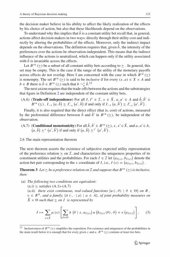
Theorem 3 Let � be a preference relation on I and suppose that Bcu (�) is inclusive,then:

(a) The following two conditions are equivalent:(a.i) � satisfies (A.1)–(A.7)(a.ii) there exist continuous, real-valued functions {u (·, θ) | θ ∈ �} on R ,v ∈ R A, and a family, {π (·, · | a) | a ∈ A}, of joint probability measures onX × � such that � on I is represented by

I →∑

x∈X

μ (x)

[∑

θ∈�

π(θ | x, aI (x)

)u

(bI (x) (θ) , θ

) + v(aI (x)

)]

, (3)

12 Inclusiveness of Bcu (�) simplifies the exposition. For existence and uniqueness of the probabilities inthe main result below it is enough that for every given x and a, Bcu (�) contains at least two bets.

123

134 E. Karni

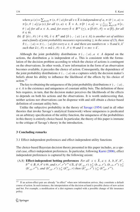
where μ (x)=∑θ∈� π (x, θ | a) for all x ∈ X is independent of a, π (θ | x, a) =

π(x, θ | a

)/μ (x) for all (x, a) ∈ X × A, π

(θ | o, a

) = 11−μ(o)

∑x∈X π

(x,

θ | a)

for all a ∈ A, and, for every b ∈ Bcu (�), u(b (θ) , θ

) = u(b), for all

θ ∈ �.(b) If {u (·, θ) | θ ∈ �}, v ∈ R A and {π (·, · | a) | a ∈ A} is another set of utilities

and a family of joint probability measures representing � in the sense of (3), thenπ (·, · | a) = π (·, · | a) for every a ∈ A and there are numbers m > 0 and k, k′such that u (·, θ) = mu (·, θ) + k , θ ∈ � and v = mv + k′.

Although the joint probability distributions π (·, · | a) , a ∈ A depend on theactions, the distribution μ is independent of a. This is consistent with the formu-lation of the decision problem according to which the choice of actions is contingenton the observations. In other words, if new information in the form of an observationbecomes available, it precedes the choice of action. Consequently, the dependence ofthe joint probability distributions π (·, · | a) on a captures solely the decision maker’sbeliefs about his ability to influence the likelihood of the effects by his choice ofaction.13

The key to obtaining the uniqueness of the joint probability distributions π (·, · | a) ,

a ∈ A is the existence and uniqueness of constant utility bets. The definition of thesebets requires, in turn, that the decision maker perceives the likelihoods of the effectsto depends on both his actions and the observations. It is worth underscoring that,neither actions nor observations can be dispense with and still obtain a choice-baseddefinition of constant utility bets.

Unlike the subjective probability in the theory of Savage (1954) (and in all othertheories that invoke Savage’s analytical framework) whose uniqueness is predicatedon an arbitrary specification of the utility function, the uniqueness of the probabilitiesin this theory is entirely choice based. In particular, the theory of this paper is immuneto the critique of Savage’s theory in the introduction.

3 Concluding remarks

3.1 Effect-independent preferences and effect-independent utility functions

The choice-based Bayesian decision theory presented in this paper includes, as a spe-cial case, effect-independent preferences. In particular, following Karni (2006), effectindependent preferences is captured by the following axiom:

(A.8) Effect-independent betting preferences For all x ∈ X , a ∈ A, b, b′, b′′,b′′′ ∈ B, θ, θ ′ ∈�, and r, r ′, r ′′r ′′′ ∈R, if (b′−θ , r) �x

a (b−θ , r ′), (b−θ , r ′′) �xa

(b′−θ , r ′′′), and (b′′−θ ′ , r ′) �x

a (b′′′−θ ′ , r) then (b′′

−θ ′ , r ′′) �xa (b′′′

−θ ′ , r ′′′).

13 If an action-effect pair are already “in effect” when new information arrives, they constitute a defaultcourse of action. In such instance, the interpretation of the decision at hand is possible choice of new actionand bet. For example, a modification of a diet regimen coupled with a possible change of life insurancepolicy.

123


The interpretation of this axiom is analogous to that of action-independent bet-ting preferences. The preferences (b′−θ , r ′) �x

a (b−θ , r) and (b−θ , r ′′) �xa (b′−θ , r ′′′)

indicate that, for every given (a, x), the “intensity” of the preference for r ′′ over r ′′′given the effect θ is sufficiently greater than that of r over r ′ as to reverse the order ofpreference between the payoffs b′−θ and b−θ . Effect independence requires that theseintensities not be contradicted by the preferences between the same payoffs given anyother effect θ.

Adding axiom (A.8) to the hypothesis of Theorem 3 implies that the utility func-tion that figures in the representation takes the form u (b (θ) , θ) = t (θ) u (b (θ)) +s (θ) , where t (θ) > 0. In other words, even if the preference relation exhibits effect-independence over bets, the utility function may still display effect dependence, inthe form of the additive and multiplicative coefficient. Thus, effects may impact thedecision maker’s well-being without necessarily affecting his risk preferences.

Let Bc be the subset of constant bets (that is, trivial bets with the same payoffregardless of the effect that obtains). If the set of constant utility bets coincides withthe set of constant bets (that is, Bc = Bcu (�)), then the utility function is effect inde-pendent (that is, u (b (θ) , θ) = u (b (θ)) for all θ ∈ �). The implicit assumption thatthe set of constant utility bets coincides with the set of constant bets is the conventioninvoked by the standard subjective utility models. Unlike in those models, however,in the theory of this paper, this assumption is a testable hypothesis.

3.2 Conditional preferences and dynamic consistency

The specification of the decision problem implies that, before the decision makerchooses an action-bet pair, either no informative signal arrives (that is, the observationis o) or new informative signal arrives in the form of an observation x ∈ X. One way oranother, given the information at his disposal, the decision maker must choose amongaction-bet pairs. Let

(�x)x∈X be binary relations on A × B depicting the decision

maker’s choice behavior conditional on observing x . I refer to(�x)

x∈X by the nameex-post preference relations.

Dynamic consistency requires that at each x ∈ X , the decision maker implementshis plan of action envisioned for that contingency by the original strategy. Formally,

Definition 4 A preference relation � on I is dynamically consistent with the ex-postpreference relations

(�x)x∈X on A × B if the posterior preference relations (�x )x∈X

satisfy �x= �x for all x ∈ X .

The following is an immediate implication of Theorem 3.

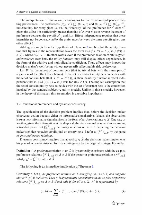
Corollary 5 Let � be preference relation on I satisfying (A.1)–(A.7) and supposethat Bcu (�) is inclusive. Then � is dynamically consistent with the ex-post preferencerelations

(�x)x∈X on A × B if and only if, for all x ∈ X , �x is represented by

(a, b) →∑

θ∈�

π (θ | x, a) u (b (θ), θ) + v (a), (4)

123

136 E. Karni

where {u (·, θ) | θ ∈ �} and {π (· | x, a) | x ∈ X , a ∈ A} are the utility functionsand conditional subjective probabilities that appear in the representation (3).

For every a ∈ A the subjective action-contingent prior on � is π (· | o, a) and thesubjective action-contingent posteriors on � are π (· | x, a) , x ∈ X. The subjectiveaction-dependent prior is the marginal distribution on � induced by the distribution onX × �, and the subjective action-dependent posteriors are obtained from the action-contingent joint distribution on X × � by conditioning on the observation.

4 Proof of Theorem 3

For expository convenience, I write Bcu instead of Bcu (�) .

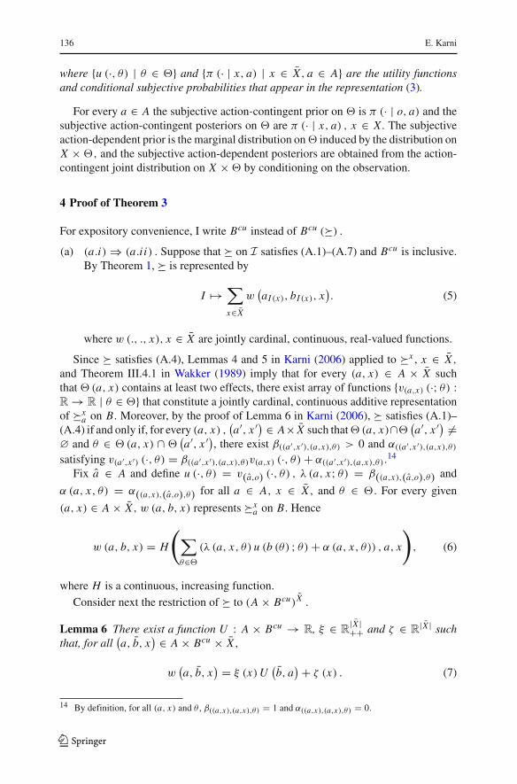
(a) (a.i) ⇒ (a.i i) . Suppose that � on I satisfies (A.1)–(A.7) and Bcu is inclusive.By Theorem 1, � is represented by

I →∑

x∈X

w(aI (x), bI (x), x

). (5)

where w (., ., x), x ∈ X are jointly cardinal, continuous, real-valued functions.

Since � satisfies (A.4), Lemmas 4 and 5 in Karni (2006) applied to �x , x ∈ X ,

and Theorem III.4.1 in Wakker (1989) imply that for every (a, x) ∈ A × X suchthat �(a, x) contains at least two effects, there exist array of functions {v(a,x) (·; θ) :R → R | θ ∈ �} that constitute a jointly cardinal, continuous additive representationof �x

a on B. Moreover, by the proof of Lemma 6 in Karni (2006), � satisfies (A.1)–(A.4) if and only if, for every (a, x) ,

(a′, x ′) ∈ A× X such that �(a, x)∩�

(a′, x ′) =

∅ and θ ∈ �(a, x) ∩ �(a′, x ′), there exist β((a′,x ′),(a,x),θ) > 0 and α((a′,x ′),(a,x),θ)

satisfying v(a′,x ′) (·, θ) = β((a′,x ′),(a,x),θ)v(a,x) (·, θ) + α((a′,x ′),(a,x),θ).14

Fix a ∈ A and define u (·, θ) = v(a,o) (·, θ) , λ (a, x; θ) = β((a,x),(a,o),θ) and

α (a, x, θ) = α((a,x),(a,o),θ) for all a ∈ A, x ∈ X , and θ ∈ �. For every given

(a, x) ∈ A × X , w (a, b, x) represents �xa on B. Hence

w (a, b, x) = H

(∑

θ∈�

(λ (a, x, θ) u (b (θ) ; θ) + α (a, x, θ)) , a, x

)

, (6)

where H is a continuous, increasing function.

Consider next the restriction of � to (A × Bcu)X .

Lemma 6 There exist a function U : A × Bcu → R, ξ ∈ R|X |++ and ζ ∈ R

|X | suchthat, for all

(a, b, x

) ∈ A × Bcu × X ,

w(a, b, x

) = ξ (x) U(b, a

) + ζ (x) . (7)

14 By definition, for all (a, x) and θ , β((a,x),(a,x),θ) = 1 and α((a,x),(a,x),θ) = 0.

123


Proof Let I, I ′, I ′′, I ′′′ ∈ I, a, a′, a′′, a′′′ ∈ A and b be as in Definition 2. Then,for all x, x ′ ∈ X , I−x

(a, b

) ∼ I ′−x

(a′, b

), I−x

(a′′, b

) ∼ I ′−x

(a′′′, b

), I ′′

−x ′(a, b

) ∼I ′′′−x ′

(a′, b

)and I ′′

−x ′(a′′, b

) ∼ I ′′′−x ′

(a′′′, b

). By the representation (5), I−x

(a, b

) ∼I ′−x

(a′, b

)implies that

∑

y∈X−{x}w

(aI (y), bI (y), y

)+w(a, b, x

)=∑

y∈X−{x}w

(aI ′(y), bI ′(y), y

)+w(a′, b, x

).

(8)

Similarly, I−x(a′′, b

) ∼ I ′−x

(a′′′, b

)implies that

∑

y∈X−{x}w

(aI(y), bI(y), y

)+w(a′′, b, x

)=∑

y∈X−{x}w

(aI ′(y), bI ′(y), y

)+w(a′′′, b, x

),

(9)

I ′′−x ′

(a, b

) ∼ I ′′′−x ′

(a′, b

)implies that

∑

y∈X−{x ′}w

(aI ′′(y), bI ′′(y), y

) + w(a, b, x ′)

=∑

y∈X−{x ′}w

(aI ′′′(y), bI ′′′(y), y

) + w(a′, b, x ′) , (10)

and I ′′−x ′

(a′′, b

) ∼ I ′′′−x ′

(a′′′, b

)implies that

∑

y∈X−{x ′}w

(aI ′′(y), bI ′′(y), y

)+w(a′′, b, x ′)

=∑

y∈X−{x ′}w

(aI ′′′(y), bI ′′′(y), y

)+w(a′′′, b, x ′). (11)

But (8) and (9) imply that

w(a, b, x

) − w(a′, b, x

) = w(a′′, b, x

) − w(a′′′, b, x

). (12)

and (10) and (11) imply that

w(a, b, x ′) − w

(a′, b, x ′) = w

(a′′, b, x ′) − w

(a′′′, b, x ′). (13)

Define a function φ(x,x ′,b) as follows: w(·, b, x

) = φ(x,x ′,b) ◦ w(·, b, x ′) . Axiom

(A.7) with b = b′ imply that it is monotonic increasing. Then φ(x,x ′,b) is continuous.Moreover, (12) and (13) in conjunction with Lemma 4.4 in Wakker (1987) imply thatφ(x,x ′,b) is affine.

123

138 E. Karni

Let β(x,o,b) > 0 and δ(x,o,b) denote, respectively, the multiplicative and additivecoefficients corresponding to φ(x,o,b), where the inequality follows from the mono-

tonicity of φ(x,o,b). Observe that, by (A.6), I−o(a, b

) ∼ I ′−o

(a′, b

)if and only if

I−o(a, b′) ∼ I ′−o

(a′, b′) . Hence

β(x,o,b)

[w

(a, b, o

) − w(a′, b, o

)] = β(x,o,b′)[w

(a, b′, o

) − w(a′, b′, o

)](14)

for all b, b′ ∈ Bcu . Thus, for all x ∈ X and b, b′ ∈ Bcu, β(x,o,b) = β(x,o,b′) :=ξ (x) > 0.

Let a, a′ ∈ A and b, b′ ∈ Bcu satisfy(a, b

) ∼o(a′, b′) . By axiom (A.7)

(a, b

) ∼o(a′, b′) if and only if

(a, b

) ∼o(a′, b′) . By the representation this equivalence implies

that

w(a, b, o

) = w(a′, b′, o

). (15)

if and only if,

ξ (x) w(a, b, o

) + δ(x,o,b) = ξ (x) w(a′, b′, o

) + δ(x,o,b′). (16)

Thus δ(x,o,b) = δ(x,o,b′).By this argument and continuity (A.2) the conclusion can be extended to Bcu . Let

δ(x,o,b) := ζ (x) for all b ∈ Bcu .

For every given b ∈ Bcu and all a ∈ A, define U(b, a

) = w(a, b, o

). Then, for

all x ∈ X ,

w(a, b, x

) = ξ (x) U(b, a

) + ζ (x) , ξ (x) > 0. (17)

This completes the proof of Lemma 6. ��

Equations (6) and (7) imply that for every x ∈ X , b ∈ Bcu and a ∈ A,

ξ (x) U(b, a

) + ζ (x) = H

(∑

θ∈�

λ (a, x, θ) u(b (θ) , θ

) + α (a, x) , a, x

)

. (18)

Lemma 7 The identity (18) holds if and only if u(b (θ) , θ

) = u(b)

for all θ ∈ �,∑

θ∈�λ(a,x,θ)

ξ(x)= ϕ (a), α(a,x)

ξ(x)= v (a) for all a ∈ A,

H

(∑

θ∈�

λ (a, x, θ) u(b (θ) , θ

)+α (a, x) , a, x

)

=ξ (x)[u

(b)+v (a)

]+ζ (x),

(19)

123


and there is κ (a) > 0 such that

κ (a)∑

θ∈�

λ (a, x, θ)

ξ (x)u

(b (θ) , θ

) + α (a, x)

ξ (x)= U

(b, a

). (20)

Proof (Sufficiency) Let u(b (θ) , θ

) := u(b)

for all θ ∈ �,∑

θ∈�λ(a,x,θ)

ξ(x):= ϕ (a)

and c (a) := κ (a) ϕ (a) for all a ∈ A and suppose that (20) holds.But axiom (A.6) and the representation imply that, for all b, b′ ∈ Bcu,

c (a) u(b) + v (a) = c

(a′) u

(b) + v

(a′)

if and only if

c (a) u(b′) + v (a) = c

(a′) u

(b′) + v

(a′).

Hence c (a) = c(a′) = c for all a, a′ ∈ A.

Normalize u so that c = 1. Then Eq. (18) follows from Eqs. (19) and (20).(Necessity) Multiply and divide the first argument of H by ξ (x) > 0. Equation (18)

may be written as follows:

ξ (x) U(b, a

)+ζ (x)= H

(

ξ (x)

[∑

θ∈�

λ (a, x, θ)

ξ (x)u

(b (θ) , θ

)+ α (a, x)

ξ (x)

]

, a, x

)

.

(21)

Define V(a, b, x

) = ∑θ∈�

λ(a,x,θ)ξ(x)

u(b (θ) , θ

) + α(a,x)ξ(x)

then, for every given

(a, x) ∈ A × X and all b, b′ ∈ Bcu ,

U(b′, a

)−U(b, a

)=[H

(ξ(x)V

(a, b′, x

), a, x

)

−H(ξ(x)V

(a, b, x

), a, x

)]/ξ

(x). (22)

Hence H (·, a, x) is a linear function whose intercept is ζ (x) and the slope

[U

(b′, a

) − U(b, a

)]/[V

(a, b′, x

) − V(a, b, x

)] := κ (a) ,

is independent of x . Thus

ξ (x) U(b, a

)+ζ (x)=κ (a) ξ (x)

[∑

θ∈�

λ (a, x, θ)

ξ (x)u

(b (θ) , θ

)+ α (a, x)

ξ (x)

]

+ζ (x).

(23)

Hence

U(b, a

)/κ (a) =

∑

θ∈�

λ (a, x, θ)

ξ (x)u

(b (θ) , θ

) + α (a, x)

ξ (x)(24)

123

140 E. Karni

is independent of x . However, because �xa =�x ′

a for all a and some x, x ′ ∈ X , in gen-eral, λ (a, x, θ) /ξ (x) is not independent of θ. Moreover, because α (a, x) /ξ (x) isindependent of b, the first term on the right-hand side of (24) must be independent of x .

For this to be true u(b (θ) , θ

)must be independent of θ and

∑θ∈� λ (a, x, θ) /ξ (x) :=

ϕ (a) be independent of x . Moreover, because the first term on the right-hand side of(24) is independent of x, α (a, x) /ξ (x) must also be independent of x . Finally, bydefinition, b the unique element in its equivalence class that has the property thatu

(b (θ) , θ

)is independent of θ .

Definev (a) := α (a, x) /ξ (x), u(b (θ) , θ

) = u(b), for all θ ∈ �, andU

(b, a

) =u

(b) + v (a) and κ (a) ϕ (a) = 1. Thus

U(b, a

) = κ (a)∑

θ∈�

λ (a, x, θ)

ξ (x)u

(b (θ) ; θ

) + α (a, x)

ξ (x). (25)

This completes the proof of Lemma 7. ��Note that

U(b, a

) =∑

θ∈�

λ (a, x, θ)

ξ (x) ϕ (a)u

(b (θ) ; θ

) + α (a, x)

ξ (x)= u

(b) + v (a) . (26)

But, by Lemma 7,∑

θ∈� λ (a, x, θ) = ξ (x) ϕ (a) . Hence, by the inclusivity of Bcu,

the representation (5) is equivalent to

I →∑

x∈X

[∑

θ∈�

λ(aI (x), x, θ

)

∑θ∈� λ

(aI (x), x, θ

)u(bI (x) (θ) ; θ

) + α(aI (x), x

)

ξ (x)

]

. (27)

For all x ∈ X, a ∈ A and θ ∈ �, define the joint subjective probability distributionon � × X by

π (x, θ | a) = λ (a, x, θ)∑

x ′∈X

∑θ ′∈� λ (a, x ′, θ ′)

. (28)

Since∑

θ∈� λ (a, x, θ) = ξ (x) ϕ (a), for all x ∈ X ,

∑

θ∈�

π (x, θ | a) = ξ (x) ϕ (a)∑

x ′∈X ξ (x ′) ϕ (a)= ξ (x)

∑x ′∈X ξ (x ′)

. (29)

Define the subjective probability of x ∈ X as follows:

μ (x) = ξ (x)∑

x ′∈X ξ (x ′). (30)

Then the subjective probability of x is given by the marginal distribution on X inducedby the joint distributions π (·, · | a) on X × � and is independent of a.

123


For all θ ∈ �, define the subjective posterior and prior probability of θ, respec-tively, by

π (θ | x, a) = π (x, θ | a)

μ (x)= λ (a, x, θ)

∑θ∈� λ (a, x, θ)

(31)

and

π (θ | o, a) = λ (a, o, θ)∑

θ∈� λ (a, o, θ). (32)

Substitute in (27) to obtain the representation (3),

I →∑

x∈X

μ (x)

[∑

θ∈�

π(θ | x, aI (x)

)u

(bI (x) (θ) , θ

) + v(aI (x)

)]

. (33)

Let a ∈ A, I ∈ I and b, b′ ∈ B, satisfy I−o (a, b) ∼ I−o(a, b′) . Then, by (33),

∑

θ∈�

π (θ | o, a) u (b (θ) , θ) =∑

θ∈�

π (θ | o, a) u(b′ (θ) , θ

)(34)

and, by axiom (A.5) and (33)

∑

x∈X

μ (x)

1−μ (0)

∑

θ∈�

π (θ | x, a) u (b (θ) , θ)=∑

x∈X

μ (x)

1−μ (0)

∑

θ∈�

π (θ | x, a) u(b′ (θ) , θ

).

(35)

Thus

∑

θ∈�

[u (b (θ) , θ) − u

(b′ (θ) , θ

)][

π (θ | o, a)−∑

x∈X

μ (x)

1 − μ (0)π (θ | x, a)

]

=0.

(36)

This implies that π(θ | o, a) = ∑x∈X μ(x)π(θ | x, a)/[1 − μ(0)].

(If π(θ | o, a) >∑

x∈X μ(x)π(θ | x, a)/[1 − μ(0)] for some θ and μ(o)π(θ ′ |o, a) <

∑x∈X μ(x)π(θ ′ | x, a)/[1 − μ(0)] for some θ ′, let b, b′ ∈ B be such that

b(θ) > b(θ) and b(θ) = b(θ) for all θ ∈ � − {θ}, b′(θ ′) > b′(θ ′) and b′(θ) = b′(θ)

for all θ ∈ � − {θ ′} and I−o(a, b) ∼ I−o(a, b′). Then

∑

θ∈�

[u

(b (θ) , θ

)− u

(b′ (θ) , θ

)][

π (θ | o, a)−∑

x∈X

μ (x)

1 − μ (0)π (θ | x, a)

]

>0.

(37)

But this contradicts (A.5).)

123

142 E. Karni

(a.i i) ⇒ (a.i) . The necessity of (A.1), (A.2) and (A.3) follows from Theo-rem 1. To see the necessity of (A.4), suppose that I−x (a, b−θr) � I−x

(a, b′−θr ′) ,

I−x(a, b′−θr ′′) � I−x

(a, b−θr ′′′) , and I−x ′

(a′, b′′−θr ′) � I−x ′

(a′, b′′′−θr

). By

representation (6 )

∑

θ ′∈�−{θ}λ

(a, x, θ ′) u

(b

(θ ′) , θ ′) + λ (a, x, θ) u (r, θ)

≥∑

θ ′∈�−{θ}λ

(a, x, θ ′) u

(b′ (θ ′) , θ ′) + λ (a, x, θ) u

(r ′, θ

), (38)

∑

θ ′∈�−{θ}λ

(a, x, θ ′) u

(b′ (θ ′) , θ ′) + λ (a, x, θ) u

(r ′′, θ

)

≥∑

θ ′∈�−{θ}λ

(a, x, θ ′) u

(b

(θ ′) , θ ′) + λ (a, x, θ) u

(r ′′′, θ

), (39)

and

∑

θ ′∈�−{θ}λ

(a′, x ′, θ ′) u

(b′′ (θ ′) , θ ′) + λ

(a′, x ′, θ

)u

(r ′, θ

)

≥∑

θ ′∈�−{θ}λ

(a′, x ′, θ ′) u

(b′′′ (θ ′) , θ ′) + λ

(a′, x ′, θ

)u (r, θ). (40)


u(r ′′, θ

) − u(r ′′′, θ

) ≥∑

θ ′∈�−{θ} λ(a, x, θ ′) [

u(b

(θ ′) , θ ′) − u

(b′ (θ ′) , θ ′)]

λ (a, x, θ)

≥ u(r ′, θ

) − u (r, θ) . (41)

Inequality (40) implies

u(r ′, θ

)−u (r, θ)≥∑

θ ′∈�−{θ} λ(a′, x ′, θ ′) [

u(b′′′ (θ ′) , θ ′)−u

(b′′ (θ ′) , θ ′)]

λ (a′, x ′, θ).

(42)


u(r ′′, θ

) − u(r ′′′, θ

)≥∑

θ ′∈�−{θ} λ(a′, x ′, θ ′) [

u(b′′′ (θ ′) , θ ′)−u

(b′′ (θ ′) , θ ′)]

λ (a′, x ′, θ).

(43)

123


Hence∑

θ ′∈�−{θ}λ

(a′, x ′, θ ′) [

u(b′′ (θ ′) , θ ′) − u

(b′′′ (θ ′) , θ ′)]

+ λ(a′, x ′, θ

) [u

(r ′′, θ

) − u(r ′′′, θ

)] ≥ 0. (44)

Thus, I−x ′(a′, b′′−θr ′′) � I−x ′

(a′, b′′′−θr ′′′) .

Next I show that if b ∈ B satisfies u(b (θ) , θ

) = u(b)

for all θ ∈ � then b ∈ Bcu .Suppose that representation (3) holds and let I, I ′, I ′′, I ′′′ ∈ I, a, a′, a′′, a′′′ ∈ Aand x, x ′ ∈ X , such that I−x

(a, b

) ∼ I ′−x

(a′, b

), I ′−x

(a′′, b

) ∼ I−x(a′′′, b

)and

I ′′−x ′

(a′, b

) ∼ I ′′′−x ′

(a, b

). Then the representation (5) implies that

∑

x∈X−{x}w

(aI(x), bI(x), x

)+ μ (x)

[u

(b) + v (a)

]

=∑

x∈X−{x}w

(aI ′(x), bI ′(x), x

)+ μ (x)

[u

(b) + v

(a′)] (45)

∑

x∈X−{x}w

(aI ′(x), bI ′(x), x

)+ μ (x)

[u

(b) + v

(a′′)]

=∑

x∈X−{x}w

(aI(x), bI(x), x

)+ μ (x)

[u

(b) + v

(a′′′)] (46)

and∑

x∈X−{x ′}w

(aI ′′(x), bI ′′(x), x

)+ μ

(x ′) [

u(b) + v

(a′)]

=∑

x∈X−{x ′}w

(aI ′′′(x), bI ′′′(x), x

)+ μ

(x ′) [

u(b) + v (a)

]. (47)


v (a) − v(a′) = v

(a′′) − v

(a′′′). (48)

Equality (47) implies

∑x∈X−{x ′}

[w

(aI ′′(x), bI ′′(x), x

)−w

(aI ′′′(x), bI ′′′(x), x

)]

μ (x ′)=v (a)−v

(a′). (49)

Thus∑

x∈X−{x ′}w

(aI ′′(x), bI ′′(x), x

)+ u

(b) + v

(a′′′) =

∑

x∈X−{x ′}w

(aI ′′′(x), bI ′′′(x), x

)

+ u(b) + v

(a′′) (50)

123

144 E. Karni

Hence I ′′−x ′

(a′′′, b

) ∼ I ′′′−x ′

(a′′′, b

)and b ∈ Bcu .

To show the necessity of (A.5) let a ∈ A, I ∈ I and b, b′ ∈ B, by the representationI−o (a, b) ∼ I−o

(a, b′) if and only if

∑

θ∈�

π (θ | o, a) u (b (θ) , θ) =∑

θ∈�

π (θ | o, a) u(b′ (θ) , θ

). (51)

But π (θ | o, a) = ∑x∈X μ (x) π (θ | x, a) / [1 − μ (0)] . Thus (51) holds if and only

if

∑

x∈X

μ (x)∑

θ∈�

π (θ | x, a) u (b (θ) , θ)=∑

x∈X

μ (x)∑

θ∈�

π (θ | x, a) u(b′ (θ) , θ

).

(52)

But (52) is valid if and only if I −o (a, b) ∼ I −o(a, b′) .

For all I and x, let K (I, x) = ∑y∈X−{x} μ

(y)[∑

θ∈� π(θ | x, a

)u(b

I(

y)(θ

)) +v(a

I(

y))]. To show the necessity of (A.6) Then I−x

(a, b

) � I ′−x

(a′, b

)if and only if

K (I, x) + u(b) + v (a) ≥ K (I ′, x) + u

(b) + v

(a′) (53)

if and only if

K (I, x) + u(b′) + v (a) ≥ K (I ′, x) + u

(b′) + v

(a′) (54)

if and only if I−x(a, b′) � I ′−x

(a′, b′) .

To show that axiom (A.7) is implied, not that I−x(a, b

) � I ′−x

(a′, b′) if and only

if

K (I, x) + u(b) + v (a) ≥ K (I, x) + u

(b′) + v

(a′) (55)

if and only if

K (I, x ′) + u(b) + v (a) ≥ K (I, x ′) + u

(b′) + v

(a′) (56)

if and only if I−x ′(a, b

) � I ′−x ′

(a′, b′) . This completes the proof of part (a).

(b) Suppose, by way of negation, that there exist continuous, real-valued functions{u (·, θ) | θ ∈ �} on R, v ∈ R

A and, for every a ∈ A, there is a joint probabilitymeasure π (·, · | a) on X ×�, distinct from those that figure in the representation (3),such that � on I is represented by

I →∑

x∈X

μ (x)

[∑

θ∈�

π(θ | x, aI (x)

)u

(bI (x) (θ) , θ

) + v(aI (x)

)]

, (57)

123


where μ (x) = ∑θ∈� π (x, θ | a) for all x ∈ X , and π (θ | x, a) = π (x, θ | a) /μ (x)

for all (θ, x, a) ∈ � × X × A.Define κ (x) = μ (x) /μ (x) , for all x ∈ X . Then the representation (57) may be

written as

I →∑

x∈X

μ (x)

[∑

θ∈�

π(θ | x, aI (x)

)γ

(θ, x, aI (x)

)κ (x) u

(bI (x) (θ) , θ

)

+ κ (x) v(aI (x)

)]

. (58)

Hence, by (3), u (b (θ) , θ) = u (b (θ) , θ) /γ (θ, x, a) κ (x) and v (a) = v (a) /κ (x).

The second equality implies that κ (x) = κ for all x ∈ X . Consequently, the firstinequality implies that γ (θ, x, a) = γ (θ) for all (x, a) ∈ X × A. Thus, for b ∈ Bcu,

I →∑

x∈X

μ (x)

[∑

θ∈�

π(θ | x, aI (x)

) u(b)

γ (θ)+ v

(aI (x)

)]

. (59)

Let b ∈ B be defined by u(

b (θ) , θ)

= u(b)/γ (θ) for all θ ∈ �. Then, b ∼x

a b

for all (x, a) ∈ X × A, and, by Definition 2, b ∈ Bcu . Moreover, if γ (·) is not aconstant function then b = b. This contradicts the uniqueness of b in Definition 2.Thus γ (θ) = γ for all θ ∈ �. But

1 =∑

x∈X

∑

θ∈�

π(θ, x | aI (x)

) = γ∑

x∈X

∑

θ∈�

π (θ, x | a) = γ. (60)

Hence, π (θ, x | a) = π (θ, x | a) for all (θ, x) ∈ � × X and a ∈ A.

Next consider the uniqueness of the utility functions. The representations (3) and(5) imply that

w (a, b, x) = μ (x)

[∑

θ∈�

π (θ | x, a) u (b (θ) , θ) + v (a)

]

. (61)

Hence, by the uniqueness part of Theorem 1, {u (·, θ)}θ∈� and v ∈ R A must satisfy

∑

θ∈�

π (θ | x, a) v (b (θ) , θ) + v (a) = m

[∑

θ∈�

π (θ | x, a) u (b (θ) , θ) + v (a)

]

+ K (x) , (62)

where m > 0. Clearly, this is the case if u (·, θ) = mu (·, θ) + k and v = mv + k′.Suppose that u (·, θ) = mu (·, θ)+ k, v = m′v + k′ and, without loss of generality,

let m > m′ > 0. Take a, a′ ∈ A and b, b′ ∈ Bcu such that(a, b

) ∼x(a′, b′) . Then,

123

146 E. Karni

by the representation (3),

u(b) − u

(b′) = v (a) − v

(a′) . (63)

But

u(b) − u

(b′) = m

[u

(b) − u

(b′)] > m′ [v (a) − v

(a′)] = v (a) − v

(a′) . (64)

Hence u (·, θ) and v do not represent � .

Consider next u (·, θ) = mu (·, θ) + k (θ) , where k (·) is not a constant function.Let k (x, a) = ∑

θ∈� π (θ | x, a) k (θ) . Take a, a′ ∈ A and b, b′ ∈ Bcu such that(a, b

) ∼x(a′, b′) and

[k (x, a) − k

(x, a′)] = 0 for some x . Then

u(b) − u

(b′) = m

[u

(b) − u

(b′)] + [

k (x, a) − k(x, a′)] = m

[v (a) − v

(a′)]

= v (a) − v(a′) .

Hence u (·, θ) and v do not represent � .

If v (a) = mv (a)+ k′ (a) , where k′ (·) is not a constant function then, by a similarargument, u (·, θ) and v do not represent � . ��Acknowledgments I am grateful to Tsogbadral Galaabaatar, Jacques Drèze, Robert Nau and an anony-mous referee for their useful comments and suggestions.

References

Anscombe, F., Aumann, R.: A definition of subjective probability. Ann Math Stat 34, 199–205 (1963)Drèze, J.H.: Les fondements logiques de l’utilite cardinale et de la probabilite subjective, pp. 73–87.

La Decision, Colloques Internationaux de CNRS (1961)Drèze, J.H.: Decision theory with moral hazard and state-dependent preferences. In: Drèze, J.H. (ed.) Essays

on Economic Decisions Under Uncertainty. Cambridge: Cambridge University Press (1987)Karni, E.: Subjective expected utility theory without states of the world. J Math Econ 42, 325–342 (2006)Karni, E.: A new approach to modeling decision-making under uncertianty. Econ Theory 33, 225–242 (2007)Karni, E.: Agency theory: choice-based foundations of the parametrized distribution formulation. Econ

Theory 36, 337–351 (2008a)Karni, E.: On optimal insurance in the presence of moral hazard. Geneva Risk Insur Rev 33, 1–18 (2008b)Machina, M.J., Schmeidler, D.: A more robust definition of subjective probability. Econometrica 60, 745–

780 (1992)Machina, M.J., Schmeidler, D.: Bayes without Bernoulli: simple conditions for probabilistically sophisti-

cated choice. J Econ Theory 67, 106–128 (1995)Mirrlees, J.: Notes on welfare economics, information and uncertainty. In: Balch, M., McFadden, D.,

Wu, S. (eds.) Essays in Economic Behavior Under Uncertainty. Amsterdam: North-Holland (1974)Mirrlees, J.: The optimal structure of authority and incentives within an organization. Bell J Econ 7,

105–113 (1976)Savage, L.J.: The Foundations of Statistics. New York: Wiley (1954)Wakker, P.P.: Subjective probabilities for state dependent continuous utility. Math Soc Sci 14, 289–298

(1987)Wakker, P.P.: Additive Representations of Preferences. Dordrecht: Kluwer (1989)

123

Copyright of Economic Theory is the property of Springer Science & Business Media B.V. and its content may

not be copied or emailed to multiple sites or posted to a listserv without the copyright holder's express written

permission. However, users may print, download, or email articles for individual use.

a theory of bayesian decision making with action-dependent

Documents