Buyer Group and Buyer Power When SellersCompete

Doh-Shin Jeon∗ and Domenico Menicucci†

November 2, 2017

Abstract

We study how buyer group affects buyer power when sellers compete with non-linear tariffs and buyers operate in separate markets. In the baseline model of twosymmetric sellers and two symmetric buyers, we characterize the set of equilibriaunder buyer group, the set without buyer group and compare both. We find that theinterval of each buyer’s equilibrium payoffs without buyer group is a strict subsetof the interval under buyer group if each seller’s cost function is strictly convex,whereas the two intervals are identical if the cost function is concave. Our resultimplies that buyer group has no effect when the cost function is concave. When itis strictly convex, buyer group strictly reduces the buyers’payoff as long as, underbuyer group, we select the Pareto-dominant equilibrium in terms of the sellers’payoffs. We extend this result to asymmetric settings with an arbitrary number ofbuyers.Keywords: Buyer Group, Buyer Power, Competition in Non-linear Tariffs,

Discriminatory Offers, Common Agency.JEL numbers: D4, K21, L41, L82

∗Toulouse School of Economics, University of Toulouse Capitole (IDEI) and CEPR.dohshin.jeon@gmail.com†Corresponding author: Università degli Studi di Firenze, Dipartimento di Scienze per l’Economia

e l’Impresa, Via delle Pandette 9, I-50127 Firenze, Italy; phone: +39-055-2759666, email:domenico.menicucci@unifi.it

1 Introduction

Does buyer group lead to buyer power? Do large buyers obtain size-related discountsfrom their suppliers? Examples of buyer groups abound in retailing (Inderst and Shaffer,2007, Caprice and Rey, 2015), health care (Marvel and Yang, 2008), cable TV (Chiptyand Snyder, 1999), academic journals (Jeon and Menicucci, 2017) etc. Understandinghow buyer group or buyer size affects buyer power is very important as policy makersin Europe and in U.S. are concerned about buyer power due to increasing buyer marketconcentration (European Commission, 1999 and OECD, 2008).1

Even if there is a large literature addressing the above questions both theoreticallyand empirically, the literature provides nuanced answers such that large-buyer discountsdo not arise under all circumstances but only under certain conditions. For instance,Chipty and Snyder (1999) and Inderst and Wey (2007) consider bargaining between amonopolist seller and each among multiple buyers and find that buyer group increases(reduces) the total payoff of the group members if the seller’s cost function is convex(concave). Inderst and Wey (2003) study a two-seller-two-buyer game which results ineach agent earning his Shapley value, and find the same result.2 Although the finding ofChipty and Snyder (1999) is confirmed in a laboratory experiment (Normann, Ruffl e, B.and Snyder, 2007), it is not confirmed by real world data as Ellison and Snyder (2010)find that in the U.S. wholesale pharmaceutical industry, large-buyer discounts can existonly if buyers face competing sellers.In this paper, we consider a setting in which sellers producing substitutes compete by

offering personalized non-linear tariffs and study how buyer group affects each player’spayoff. As in Chipty and Snyder (1999) and Inderst and Wey (2003, 2007), we do notconsider competition among buyers: each buyer operates in a separate market. Aftershowing that all equilibria are effi cient regardless of whether or not the buyers form agroup (Proposition 1), we consider a baseline model with two symmetric sellers and twosymmetric buyers. We characterize the set of equilibria that arise under buyer group(Section 3), the set of equilibria that arise without buyer group (Section 4), and comparethese sets (Section 5). All equilibria can be ranked according to the payoff of each buyer,and we find that the interval of each buyer’s equilibrium payoffs without buyer group isa strict subset of the interval under buyer group if each seller’s cost function is strictlyconvex, whereas the two intervals are identical if the cost function is concave.

1In US, the Federal Trade Commission organized in 2000 a workshop on slotting allowances, a majorbuyer power issue in grocery retailing. See Chen (2007) for a survey of the literature on buyer power andantitrust policy implications.

2More broadly, in cooperative game theory there is a literature on joint bargaining parodox (Harsanyi,1977) or collusion neutrality (van den Brink, 2012), which studies when a coalition formation increasesor reduces the joint payoff of its members from bargaining.

1

This finding suggests that buyer group has no effect on the buyers’payoff when thesellers’cost function is concave. When it is strictly convex, buyer group can increase ordecrease the buyers’payoff depending on the equilibrium selection. If we select, underbuyer group, the equilibrium which is Pareto-dominant in terms of the sellers’payoffs as inBernheim andWhinston (1986, 1998),3 our result implies that buyer group strictly reducesthe buyers’payoff no matter the equilibrium played without buyer group. Therefore, wecan conclude that buyer group does not increase the buyers’payoff regardless of whetherthe sellers’cost function is convex or concave. Then we generalize the result obtainedfrom the baseline model with convex cost: we consider two asymmetric sellers and n(≥ 2)

asymmetric buyers and show that as long as a seller’s cost function is strictly convex, in anyequilibrium without buyer group, the buyers obtain a strictly higher total payoff(and eachseller obtains a strictly lower payoff) than in the Pareto-dominant equilibrium for sellersunder buyer group (Proposition 5). We notice that the Pareto-dominant equilibrium forsellers under buyer group is also called a "sell-out equilibrium" by Bernheim andWhinston(1998).4

We below provide the intuition for our result in the baseline model regarding theequilibrium which is Pareto-dominant in terms of the sellers’payoffs. It is well-known fromBernheim and Whinston (1998) that in the equilibrium under buyer group, each seller jis indifferent between inducing the group to buy from both sellers (as in equilibrium) andinducing the group to buy exclusively from seller j. The latter strategy is equivalent tothe strategy, without the group, that induces both buyers to buy exclusively from seller j.However, when there is no group, seller j can also deviate by inducing only one buyer tobuy exclusively from himself while inducing the other buyer to keep buying the equilibriumquantity from the rival seller. No buyer group reduces the sellers’(best) payoff (and henceincreases the buyers’(worst) payoff)5 if and only if the deviation inducing both buyersto buy exclusively is less powerful than the deviation inducing only one buyer to buyexclusively. Note that inducing both buyers to buy exclusively requires a larger increasein output of j than inducing only one buyer to buy exclusively. Therefore, when the costfunction is strictly convex, because of increasing marginal costs, if the deviation inducingonly one buyer to buy exclusively is not profitable, the deviation inducing both buyersto buy exclusively is not profitable either. However, the reverse does not hold and if aseller is indifferent between no deviation and the deviation inducing both buyers to buyexclusively, the deviation inducing only one buyer to buy exclusively becomes profitable

3The equilibrium is also the truthful equilibrium under buyer group.4In the sell-out equilibrium, each seller j uses a sell-out strategy such that the payment of the buyer

group for purchasing quantity qj takes the form of Fj +Cj(qj), where Fj is a fixed fee and Cj is j’s costfunction.

5Since all equilibria are effi cient, a decrease in the sellers’payoff implies an increase in the buyers’payoff.

2

since the marginal cost increases less due to smaller output expansion. A similar reasoningimplies that when the cost function is concave, if the deviation inducing both buyers tobuy exclusively is not profitable, the deviation inducing only one buyer to buy exclusivelyis not profitable. Therefore, buyer group reduces the buyers’(worst) payoff if the costfunction is strictly convex while it does not affect it if the cost function is concave.6

A big picture consistent with some empirical findings emerges when our results arecombined with the findings of Inderst and Shaffer (2007) and Dana (2012).7 Their modelsare similar to ours as they assume that sellers have complete information about buyers’preferences and hence compete by offering personalized tariffs, regardless of whether ornot buyers form a group. The crucial difference is that they assume that the buyer groupmakes an exclusive purchase commitment while we do not consider any such commitment.They find that a buyer group never decreases the total payoff of its members and strictlyincreases it unless the members have identical preferences. This is because group forma-tion among heterogenous buyers makes the buyers more homogenous (as a group) andthereby intensifies competition for exclusivity between sellers.Combining their result with ours leads to the following prediction: when sellers pro-

ducing substitutes compete, buyer group increases the total payoff of its members onlyif the group can pre-commit to limit its purchases to a subset of sellers. This predictionis consistent with the empirical findings of Ellison and Snyder (2010), Competition Com-mission of U.K. (2008) and Sorensen (2003). Their common findings are: buyer size alonedoes not explain discounts but it is a buyer’s credible threat to exclude certain productsfrom purchase that explains discounts. For instance, Ellison and Snyder (2010) find thatlarge buyers (chain drugstores) receive either very small or no statistically significant dis-counts relative to small buyers (independent drugstores) for off-patent antibiotics whichhave one or more generic substitutes available but that hospitals and health-maintenance

6We can also provide the intuition for our result in the baseline model regarding the equilibrium whichgenerates the worst payoff for the sellers. It turns out that in the equilibrium under buyer group, eachseller j is indifferent between inducing the group to buy the equilibrium quantity from each seller andinducing the group to buy a larger quantity from the rival, which implies that seller j sells less upon thedeviation. The latter strategy is equivalent to the strategy, without the group, that induces both buyersto buy more from the rival seller. However, when there is no group, seller j can also deviate by inducingonly one buyer to buy more from the rival. No buyer group increases the sellers’(worst) payoff and hencedecreases the buyers’(best) payoff if and only if the deviation inducing both buyers to buy more fromthe rival is less powerful than the deviation inducing only one buyer to buy more from the rival. Whenthe cost function is convex (concave), inducing a first buyer to buy more from the rival generates a larger(smaller) cost saving than inducing a second buyer to buy more from the rival. Therefore, no buyer groupdecreases the buyers’(best) payoff if the cost function is strictly convex while it does not affect it if thecost function is concave.

7See also Caprice and Rey (2015) who provide a mechanism through which buyer group among (com-peting) retailers leads to buyer power through joint delisting decision.

3

organizations (HMOs) receive substantial discounts relative to drugstores. They explainthis finding by the fact that chain drugstores and independent drugstores do not differmuch in the substitution opportunities whereas hospitals and HMOs can and do committo limit their purchases to certain drugs by issuing restrictive formularies as they cancontrol which drugs their affi liated doctors prescribe.8

Our analysis of the symmetric setting in Sections 3 and 4 has some technical contribu-tion as well. We show that any symmetric equilibrium can be replicated by an equilibriumobtained from allowing each seller to offer only two pairs of quantity and price. We usethis approach to characterize the whole set of equilibria depending on whether or not thebuyers formed a group. The approach is useful because it reduces the problem of findingall the equilibria to a relatively simple problem.9

In Section 7, we apply our insights to a situation in which one seller’s entry is endoge-nous and the buyers decide whether or not to form a group before the entry decision.10

We assume that the sellers’cost functions are strictly convex. The entrant has to incur afixed cost of entry, which is a random draw from a (commonly known) distribution as inAghion and Bolton (1987), Innes and Sexton (1994) and Chen and Shaffer (2014). Uponentry, both sellers simultaneously offer non-linear tariffs and we assume that they playthe Pareto-dominant equilibrium. Therefore, when the buyers decide to form or not agroup, they face a trade-off: forming the buyer group increases the probability of entrybut reduces the total payoff of the buyers conditional on entry. In particular, conditionalon buyer group formation, the private entry decision coincides with the socially optimalone as in the sell-out equilibrium, each firm’s profit is equal to its social marginal con-tribution. This implies that no formation of group leads to a socially suboptimal entry.The existing literature on naked exclusion explains suboptimal entry by the incumbent’staking advantage of coordination failure among buyers (Rasmusen, Ramseyer and Wiley1991, Segal and Whinston, 2000, Fumagalli and Motta, 2006, 2008, Chen and Shaffer,

8Similarly, the study of the competition commission (2008) of the U.K. grocery industry finds signifi-cant buyer-size discounts for non-primary brand goods (for which the grocer can freely substitute amongdifferent suppliers) but not for primary brand goods (for which grocers have limited substitution oppor-tunities). Sorensen (2003) also find that size alone cannot explain why some insurers get much betterdeal from hospitals than other insurers and that an insurer’s ability to channel its patients to selectedhospitals can explain why small managed care organizations are often able to extract deeper discountsfrom hospitals than very large indemnity insurers.

9This approach is adopted partly because the sell-out equilibrium (Bernheim and Whinston, 1998),which exists under buyer group, does not exist without group if the costs are strictly convex or strictlyconcave. Hence, even if we want to focus on the Pareto-dominant equilibrium, the approach is useful forthe analysis of no group.10For instance, state-wide (or multi-state) large pharmaceutical purchasing alliances (Ellison and Sny-

der, 2010) can affect entry decision of generic drug producers or a buying alliance among large chains ofsupermarkets (Caprice and Rey, 2015) can have an impact on entry of national brand manufacturers.

4

2014). While the literature typically assumes that the incumbent makes offers to buyersbefore the entry, Fumagalli and Motta (2008) show that the coordination failure surviveseven if both sellers make simultaneous offers. However, in these papers, buyers have noreason not to form a group (at least among those operating in separate markets) as thiswould remove the coordination failure. Our application shows that buyers may choosenot to form a group even if this leads to a suboptimal entry.In Section 8, we consider the case in which the two products can be substitutes or

complements while the cost functions are linear. We focus on sell-out equilibria whichexist regardless of whether or not the buyers form a group. Then, buyer group has noeffect on any player’s payoff if the products sold by the sellers are complements to bothbuyers (or substitutes to both buyers). But if the products are strict substitutes forbuyer 1 and strict complements for buyer 2, then buyer group reduces the buyers’totalpayoff. Note that the sellers have some residual market power with respect to buyer 2as each seller charges less than the incremental value of his product because charging theincremental value leads to a strictly negative payoff to buyer 2. Buyer group allows thesellers to transfer the residual market power to buyer 1 in the same way as multi-marketcontact facilitates collusion by transferring residual collusive power from one market toanother (Bernheim and Whinston, 1990).

1.1 Literature review

The literature has used various ways to generate size-related discounts. Katz (1987),Scheffman and Spiller (1992) and Inderst and Valletti (2011) model buyer power as down-stream firms’ability to integrate backwards by paying a fixed cost. Buyer group makesthis outside option stronger as the group can share the fixed cost among its members,which in turn allows the group to obtain a larger discount from a seller. The paperswhich do not consider such size-related outside option can be regrouped into two differentcategories. On the one hand, there are papers studying buyer group among competingdownstream firms. Hence, buyer group not only allows them to joins force as buyers butalso eliminates competition between them in the downstream market: see von Ungern-Sternberg (1996), Dobson and Waterson (1997), Chen (2003), Erutku (2005) and Gaudin(2017).11 On the other hand, there are papers which focus on ‘pure’ buyer power inthe sense that group members only interact on the buying side as they do not compete.The second branch of literature can be further distinguished depending on whether theyconsider a monopoly seller (Chipty and Snyder, 1999, and Inderst and Wey, 2007) orcompeting sellers (Inderst and Shaffer, 2007, Marvel and Yang, 2008, Dana, 2012, Chen

11Caprice and Rey (2015) is an exception as they consider a buyer group among retailers which maintaindownstream competition.

5

and Li, 2013). As we consider upstream competition but no downstream competition,our paper is close to the last subcategory, in particular to Inderst and Shaffer, (2007) andDana (2012). However, our paper is also related to Chipty and Snyder (1999) and Inderstand Wey (2003, 2007) in terms of prediction based on the curvature of the seller(s)’costfunction. Namely, they predict that the buyer group increases (reduces) the total payoffof the group members if the seller’s cost function is convex (concave). This occurs becausebuyers are assumed to have some bargaining power and the incremental costs to serve thegroup is smaller (larger) than the sum of the incremental cost to serve each buyer if sellers’costs are convex (concave).12 In contrast, we predict that the buyer group reduces (doesnot affect) the total payoff of the group members if the seller’s cost function is convex(concave).13

To the best of our knowledge, we are the first to analyze the effect of buyer group onbuyer power in a framework that extends the common agency (Bernheim and Whinston,1986, 1998) to multiple buyers. For the setting without buyer group, Prat and Rustichini(2003) analyze a general setup with multiple sellers and multiple buyers in which buyers’utility functions are concave and sellers’cost functions are convex. They allow sellers touse more complex tariffs than ours: seller j can make buyer i’s payment depend on thewhole vector of i’s purchases such that the payment depends on qij and also on q

ik for each

seller k different from j. They prove the existence of an effi cient equilibrium, but do notspecify the equilibrium strategies and do not compare the case of buyer group with thecase of no group. We consider tariffs such that the payment of each buyer i to each sellerj only depends on qij, the quantity buyer i buys from seller j14 and compare buyer groupwith no group.15

12In our setting, using the Shapley value to compare the buyers’payoffs under buyer group with thepayoffs under no group, yields the same results as in Inderst and Wey (2003).13The literature on buyer group is large. Snyder (1996, 1998) apply the idea of Rotemberg and Saloner

(1986) to explain why large buyers get discounts. Namely, he considers a model of tacit collusion amongsellers and shows that sellers charge lower prices to large buyers while charging monopoly prices tosmall buyers. Ruffl e (2013) test experimentally the theory and find support for it. Chae and Heidhues(2004) (DeGraba, 2005) generate large-buyer discounts from buyers’risk aversion (seller’s risk aversion).Loertscher and Marx (2017) study competitive effects of upstream merger in a market with buyer power.14There are two reasons for restricting attention to such tariff. First, a seller j may not observe

the quantity that a buyer buys from the other seller. Second, market-share contracts that provide pricerebates conditional on buying a large share of quantity from the seller making the offer are often prohibitedby antitrust authorities when practiced by dominant firms. For instance, on May 13, 2009, EuropeanCommission imposed a fine of 1.06 billion euros on Intel for such behavior.15Jeon and Menicucci (2012) extends the common agency to competition between portfolios in the

presence of the buyer’s slot constraint and provide conditions to make the "sell-out equilibrium" theunique equilibrium. Contrary to what happens under slot constraint, Jeon and Menicucci (2006) showthat in the presence of the buyer’s budget constraint, the well-known result in the common agencyliterature that competition between sellers achieves the outcome that maximizes all parties’joint payoff

6

Our paper is distantly related to our companion paper (Jeon and Menicucci, 2017)which studies library consortium in the market for academic journals. Each seller (i.e.,publisher) is a monopolist of his journals and sells a bundle of his electronic academicjournals at personalized price(s). However, we assume that each seller’s marginal costis zero such that in the absence of buyer group (i.e., library consortium), each library’smarket can be studied in isolation. Competition among sellers occurs because of thebudget constraint of each buyer. We find that depending on the sign and degree ofcorrelation between each member library’s preferences, building a library consortium canincrease or reduce the total payoffs’of the buyers.16

2 The model and a preliminary result

There are two sellers (A and B) and two buyers (1 and 2). Let qij ≥ 0 represent thequantity of the product that buyer i (= 1, 2) buys from seller j (= A,B). For each buyer i,the gross utility from consuming (qiA, q

iB) is given by U i(qiA, q

iB), with U i strictly increasing

and strictly concave in (qiA, qiB). Precisely, we let U ij = ∂U i/∂qij, U

ijk = ∂U i/∂qij∂q

ik, and

assume that for each buyer i (i) U ij > 0, but U ij → 0 as qij → +∞; (ii) the Hessian matrixof U i is negative definite, hence U i is strictly concave; (iii) U iAB < 0, hence the goodsare strict substitutes.17 For each seller j, the cost of serving the buyers is Cj(q1j + q2j ).We assume that Cj(0) = 0, Cj is strictly increasing, but Cj can be convex or concave.However, if Cj is concave, then we assume that U1, U2 are concave enough such that socialwelfare U1(q1A, q

1B) + U2(q2A, q

2B)− CA(q1A + q2A)− CB(q1B + q2B) is a concave function.

Each seller offers a non-linear tariffto each buyer (or to the buyer group). In particular,we consider tariffs such that what buyer i pays to seller j depends only on the quantitythat the buyer purchases from seller j, and not on the quantity she purchases from theother seller. When there is no buyer group, we allow each seller to offer personalized non-linear tariffs: the tariff offered by seller j to buyer i is denoted by T ij (q) (with T

ij (0) = 0),

and can be different from the tariff seller j offers to buyer h ( 6= i). After seeing the tariffs,buyer i chooses (qiA, q

iB) in order to maximize U i(qiA, q

iB)− T iA(qiA)− T iB(qiB).

When the buyers form a buyer group, the sellers compete for serving the group. LetG denote the buyer group, qGj the quantity G buys from seller j, and T

Gj (q) the non-linear

tariff that seller j offers to G (with TGj (0) = 0). We define UG(qGA , qGB) as follows:

UG(qGA , qGB) ≡ max

q1A,q1B ,q

2A,q

2B

U1(q1A, q1B) + U2(q2A, q

2B) (1)

fails to hold.16Therefore, in terms of the results, the companion paper is situationed between Inderst and Shaffer

(2007) and Dana (2012) on the one hand, and the current paper on the other hand.17We consider the case of complementary goods in Proposition 7.

7

subject to q1A + q2A = qGA , q1B + q2B = qGB . (2)

Thus UG(qGA , qGB) is the group’s gross utility from buying

(qGA , q

GB

), as it results from the

optimal allocation of(qGA , q

GB

)between the two buyers.18 Hence, after seeing the tariffs,

G chooses(qGA , q

GB

)in order to maximize UG(qGA , q

GB)− TGA (qGA)− TGB (qGB).

Define q∗ ≡ (q1∗A , q1∗B , q

2∗A , q

2∗B ) as the unique allocation vector that maximizes social

welfare,19 and V GAB as the social welfare in the first-best allocation q∗:

q∗ ≡ arg max(q1A,q1B ,q2A,q2B)

U1(q1A, q1B) + U2(q2A, q

2B)− CA(q1A + q2A)− CB(q1B + q2B), (3)

V GAB ≡ U1(q1∗A , q

1∗B ) + U2(q2∗A , q

2∗B )− CA(q1∗A + q2∗A )− CB(q1∗B + q2∗B ) (4)

We say that an equilibrium is effi cient if the equilibrium allocation is q∗. From Proposition2 to Proposition 7 below, we assume that each buyer buys a positive quantity from eachseller in the first best allocation: qi∗j > 0 for i = 1, 2 and j = A,B.20

We consider a game with the following timing:

• Stage 0: The buyers decide whether they will form a group or not.

• Stage 1: When there is no buyer group, each seller j (= A,B) simultaneouslychooses T ij (q) for i = 1, 2. When the buyer group is formed, each seller j (= A,B)simultaneously chooses TGj (q).

• Stage 2: Each buyer i, or the buyer group, makes purchase decisions.

As we are mainly interested in comparing the outcome of competition under buyergroup with the one without group, when we refer to an equilibrium, we mean an equilib-rium of the game that starts from Stage 1 with or without buyer group.We start by proving that each equilibrium is effi cient both in the case of buyer group

and in the case of no group. This

Proposition 1 (effi ciency) Any equilibrium is effi cient regardless of whether or not thebuyers form a group.

This result implies that the total quantity that the buyers buy from each seller doesnot depend on whether or not the buyers form a group. In other words, the total payoffof the buyers is completely determined by the payments they make to the sellers. Hence,

18In principle, the constraints in (2) should be written as q1A+q2A ≤ qGA , q1B +q2B ≤ qGB , but since U1, U2are strictly increasing, equality holds in the optimum.19Our assumptions imply that for each maximization problem below, a maximizer exists and is unique

since the objective function is strictly concave.20This assumption is not needed in Proposition 1.

8

if buyer group increases (reduces) the total payoff of the buyers, it is because the buyerspay less (more) for the same total quantity. This creates a natural connection to theliterature that studies buyer power defined as size-related discounts.The result for the case of buyer group is a consequence of Proposition 1 in O’Brien and

Shaffer (1997), which implies that in any equilibrium under buyer group, the equilibriumquantities, denoted by

(qGeA , qGeB

), are such that

qGeA ∈ arg maxqGA

(UG(qGA , q

GeB )− CA(qGA)

), qGeB ∈ arg max

qGB

(UG(qGeA , qGB)− CB(qGB)

).

This means that qGeA maximizes the sum of G’s payoff and firm A’s profit, given qGB = qGeB ,and an analogous property holds for qGeB . Therefore,{

UGA (qGeA , qGeB ) ≤ C ′A(qGeA ), with equality if qGeA > 0;

UGB (qGeA , qGeB ) ≤ C ′B(qGeB ), with equality if qGeB > 0.(5)

Since U1 and U2 are concave, it follows that UG is concave and social welfare UG(qGA , qGB)−

CA(qGA)−CB(qGB) is a concave function of(qGA , q

GB

)as we assumed above. The conditions

in (5) are the necessary first order conditions for maximization of social welfare, andmoreover they are suffi cient since social welfare is concave. Hence,

(qGeA , qGeB

)maximizes

social welfare, that is qGeA = q1∗A + q2∗A , qGeB = q1∗B + q2∗B .

21

A similar intuition applies also to the case of no buyer group: We can prove that inany equilibrium, the equilibrium quantities (q1eA , q

1eB , q

2eA , q

2eB ) are such that{

(q1eA , q2eA ) ∈ arg maxq1A,q2A (U1(q1A, q

1eB ) + U2(q2A, q

2eB )− CA(q1A + q2A)) ;

(q1eB , q2eB ) ∈ arg maxq1B ,q2B (U1(q1eA , q

1B) + U2(q2eA , q

2B)− CB(q1B + q2B)) .

(6)

This means that (q1eA , q2eA ) maximizes the sum of the buyers’ total payoff and firm A’s

profit, given (q1B, q2B) = (q1eB , q

2eB ), and an analogous property holds for (q1eB , q

2eB ). Since

social welfare U1(q1A, q1B)+U2(q2A, q

2B)−CA(q1A+q2A)−CB(q1B+q2B) is a concave function, it

follows from (6) that (q1eA , q1eB , q

2eA , q

2eB ) maximizes social welfare, that is (q1eA , q

1eB , q

2eA , q

2eB ) =

(q1∗A , q1∗B , q

2∗A , q

2∗B ).

In the next three sections we consider a setting in which both buyers and sellers aresymmetric, that is U1(·) = U2(·) ≡ U(·), U(qA, qB) = U(qB, qA), and CA(·) = CB(·) ≡C(·). In this setting q1∗A = q1∗B = q2∗A = q2∗B ≡ q∗ such that

Uj(q∗, q∗) = C ′(2q∗) for j = A,B (7)

21O’Brien and Shaffer (1997) exhibit a setting in which an ineffi cient equilibrium exists, but thatsetting has discontinuous cost functions for sellers (because of a fixed cost each seller bears for eachpositive quantity produced). Therefore, the social welfare function is not concave.

9

andUG(qGA , q

GB) = 2U(

1

2qGA ,

1

2qGB) (8)

We call this the symmetric setting.In the symmetric setting, we will illustrate our results through the following example:

U(qA, qB) = (q1/2A + q

1/2B )1/2 and C(q) =

1

2q2.

This implies

UA(qA, qB) =1

4q1/2A (q

1/2A + q

1/2B )1/2

and q∗ solves1

4q1/2(q1/2 + q1/2)1/2= 2q

Therefore q∗ = 14, U(q∗, q∗) = 1, C(2q∗) = 1

8, and V G

AB = 74. From (8), we have.

UG(qGA , qGB) = 23/4((qGA)1/2 + (qGB)1/2)1/2.

3 Equilibria under buyer group

In this section, we consider the symmetric setting and study the case in which buyershave formed a group G. Given the symmetric setting, we focus on symmetric equilibriasuch that each seller offers G the same tariff TGA (.) = TGB (.) ≡ TG(.).Since each equilibrium is effi cient (see Proposition 1), we know that G buys quantity

2q∗ [see (7)] from each seller in each equilibrium, and G’s payoff is uG ≡ UG(2q∗, 2q∗) −2TG(2q∗). In fact, uG is also equal to maxq≥0[U

G(0, q) − TG(q)], that is the highestpayoff G can obtain by trading only with one seller. This equality holds because ifuG < maxq≥0[U

G(0, q)−TG(q)], then buying quantity 2q∗ from each seller is not G’s bestchoice. If uG > maxq≥0[U

G(0, q)−TG(q)], then seller A (to fix the ideas) for instance canincrease his profit as follows: He makes a take-it-or-leave-it offer to G with quantity 2q∗

and payment TG(2q∗) + ε (with ε > 0 and small), and if G buys 2q∗ from each seller thenhis payoff is UG(2q∗, 2q∗) − 2TG(2q∗) − ε = uG − ε which is still larger than the highestpayoffG can make by trading only with seller B.For future reference, we let

q ∈ arg maxq≥0

[UG(0, q)− TG(q)], tG ≡ TG(q), tG∗ ≡ TG(2q∗). (9)

Hence,uG = UG(2q∗, 2q∗)− 2tG∗ = UG(0, q)− tG. (10)

10

Note that q ≥ 2q∗ should hold since 2q∗ ∈ arg maxq≥0[UG(2q∗, q)−TG(q)] and the products

are substitutes. In fact, we can prove that q > 2q∗ in each equilibrium: see the proof ofLemma 1 below.Next lemma proves that each equilibrium is characterized by (q, tG), that is G’s best

choice when trading only with a seller, such that there exists an equivalent equilibrium (interms of outcome) in which each seller offers only two contracts (2q∗, tG∗) and (q, tG).22

Note that once (q, tG) is determined, tG∗ is determined from (10). This allows to charac-terize all the equilibrium outcomes by restricting attention to a simple class of tariffs.

Lemma 1 Consider the symmetric setting with buyer group. Given any symmetric equi-librium in which each seller offers the same tariff TG, there exists an equilibrium in whicheach seller offers only two contracts (2q∗, tG∗) and (q, tG) and of which the outcome is thesame as that of the original equilibrium.

Therefore, from now on we consider the equilibrium in which each seller offers onlythe two contracts (2q∗, tG∗) and (q, tG). Suppose that seller B offers the two contracts(2q∗, tG∗) and (q, tG) but that seller A considers deviating with a take-it-or-leave-it offer(qA, tA) to G. Then G accepts the offer if and only if UG(qA, qB) − tA − TG(qB) ≥ uG

for at least one qB ∈ {0, 2q∗, q}. Thus UG(qA, qB)− TG(qB)− uG is the highest paymentseller A can obtain from G. Therefore, given qB ∈ {0, 2q∗, q}, seller A chooses qA ∈arg maxx≥0[U

G(x, qB)− TG(qB)− uG − C(x)]. For this reason, for each b ≥ 0 we define

fG(b) ≡ maxx≥0

(UG(x, b)− C(x)

). (11)

Conditional on that seller A inducesG to buy qB = b from sellerB, the deviation generatesa joint payoff of fG(b)− TG(b) for G and seller A and fG(b)− TG(b)− uG is the profit ofseller A.Next proposition identifies the set of equilibrium payoffs for G.

Proposition 2 (Equilibria with Buyer Group) Consider the symmetric setting and sup-pose that the buyers formed a group. There exists a symmetric equilibrium in which thegroup’s payoff is uG if and only if

2fG(0)− V GAB ≤ uG ≤ V G

AB − 2 limb→+∞

[fG(b)− UG(0, b)]. (12)

We below explain how the left hand side and the right hand side in (12) are obtained.First, we notice that fG(0) = maxx≥0

(UG(x, 0)− C(x)

)is the maximal social welfare

when G trades only with seller A, and in any equilibrium the sum of G’s payoff uG and

22This means that each seller chooses a tariff TG such that TG(q) is very high if q > 0, q 6= 2q∗, q 6= q.

11

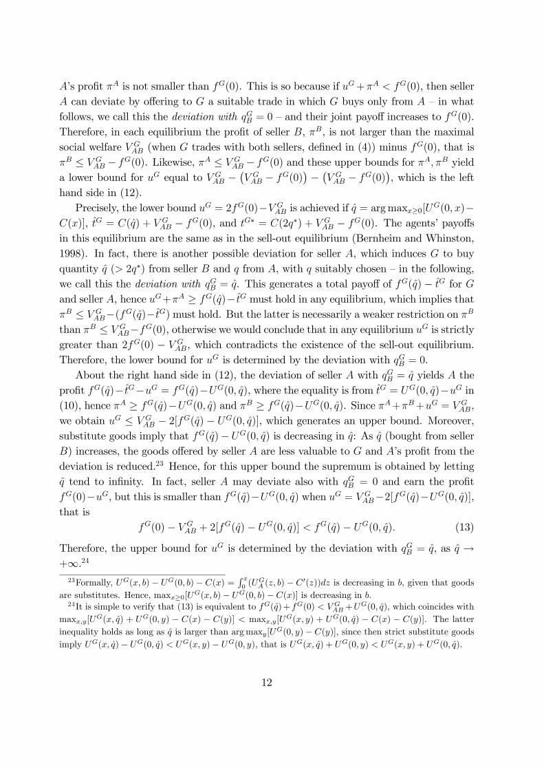
A’s profit πA is not smaller than fG(0). This is so because if uG+πA < fG(0), then sellerA can deviate by offering to G a suitable trade in which G buys only from A —in whatfollows, we call this the deviation with qGB = 0 —and their joint payoff increases to fG(0).Therefore, in each equilibrium the profit of seller B, πB, is not larger than the maximalsocial welfare V G

AB (when G trades with both sellers, defined in (4)) minus fG(0), that isπB ≤ V G

AB − fG(0). Likewise, πA ≤ V GAB − fG(0) and these upper bounds for πA, πB yield

a lower bound for uG equal to V GAB −

(V GAB − fG(0)

)−(V GAB − fG(0)

), which is the left

hand side in (12).Precisely, the lower bound uG = 2fG(0)−V G

AB is achieved if q = arg maxx≥0[UG(0, x)−

C(x)], tG = C(q) + V GAB − fG(0), and tG∗ = C(2q∗) + V G

AB − fG(0). The agents’payoffsin this equilibrium are the same as in the sell-out equilibrium (Bernheim and Whinston,1998). In fact, there is another possible deviation for seller A, which induces G to buyquantity q (> 2q∗) from seller B and q from A, with q suitably chosen —in the following,we call this the deviation with qGB = q. This generates a total payoff of fG(q)− tG for Gand seller A, hence uG+πA ≥ fG(q)− tG must hold in any equilibrium, which implies thatπB ≤ V G

AB−(fG(q)−tG)must hold. But the latter is necessarily a weaker restriction on πB

than πB ≤ V GAB−fG(0), otherwise we would conclude that in any equilibrium uG is strictly

greater than 2fG(0) − V GAB, which contradicts the existence of the sell-out equilibrium.

Therefore, the lower bound for uG is determined by the deviation with qGB = 0.About the right hand side in (12), the deviation of seller A with qGB = q yields A the

profit fG(q)− tG−uG = fG(q)−UG(0, q), where the equality is from tG = UG(0, q)−uG in(10), hence πA ≥ fG(q)−UG(0, q) and πB ≥ fG(q)−UG(0, q). Since πA+πB+uG = V G

AB,we obtain uG ≤ V G

AB − 2[fG(q) − UG(0, q)], which generates an upper bound. Moreover,substitute goods imply that fG(q)−UG(0, q) is decreasing in q: As q (bought from sellerB) increases, the goods offered by seller A are less valuable to G and A’s profit from thedeviation is reduced.23 Hence, for this upper bound the supremum is obtained by lettingq tend to infinity. In fact, seller A may deviate also with qGB = 0 and earn the profitfG(0)−uG, but this is smaller than fG(q)−UG(0, q) when uG = V G

AB−2[fG(q)−UG(0, q)],that is

fG(0)− V GAB + 2[fG(q)− UG(0, q)] < fG(q)− UG(0, q). (13)

Therefore, the upper bound for uG is determined by the deviation with qGB = q, as q →+∞.2423Formally, UG(x, b)− UG(0, b) − C(x) =

∫ x0

(UGA (z, b)− C ′(z))dz is decreasing in b, given that goodsare substitutes. Hence, maxx≥0[U

G(x, b)− UG(0, b)− C(x)] is decreasing in b.24It is simple to verify that (13) is equivalent to fG(q) + fG(0) < V GAB +UG(0, q), which coincides with

maxx,y[UG(x, q) + UG(0, y) − C(x) − C(y)] < maxx,y[UG(x, y) + UG(0, q) − C(x) − C(y)]. The latterinequality holds as long as q is larger than arg maxy[UG(0, y)− C(y)], since then strict substitute goodsimply UG(x, q)− UG(0, q) < UG(x, y)− UG(0, y), that is UG(x, q) + UG(0, y) < UG(x, y) + UG(0, q).

12

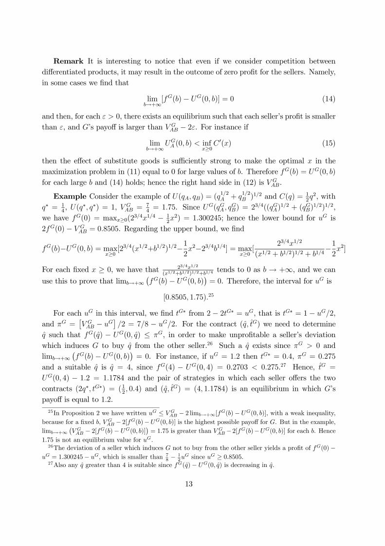
Remark It is interesting to notice that even if we consider competition betweendifferentiated products, it may result in the outcome of zero profit for the sellers. Namely,in some cases we find that

limb→+∞

[fG(b)− UG(0, b)] = 0 (14)

and then, for each ε > 0, there exists an equilibrium such that each seller’s profit is smallerthan ε, and G’s payoff is larger than V G

AB − 2ε. For instance if

limb→+∞

UGA (0, b) < infx≥0

C ′(x) (15)

then the effect of substitute goods is suffi ciently strong to make the optimal x in themaximization problem in (11) equal to 0 for large values of b. Therefore fG(b) = UG(0, b)

for each large b and (14) holds; hence the right hand side in (12) is V GAB.

Example Consider the example of U(qA, qB) = (q1/2A + q

1/2B )1/2 and C(q) = 1

2q2, with

q∗ = 14, U(q∗, q∗) = 1, V G

AB = 74

= 1.75. Since UG(qGA , qGB) = 23/4((qGA)1/2 + (qGB)1/2)1/2,

we have fG(0) = maxx≥0(23/4x1/4 − 1

2x2) = 1.300245; hence the lower bound for uG is

2fG(0)− V GAB = 0.8505. Regarding the upper bound, we find

fG(b)−UG(0, b) = maxx≥0

[23/4(x1/2+b1/2)1/2−1

2x2−23/4b1/4] = max

x≥0[

23/4x1/2

(x1/2 + b1/2)1/2 + b1/4−1

2x2]

For each fixed x ≥ 0, we have that 23/4x1/2

(x1/2+b1/2)1/2+b1/4tends to 0 as b → +∞, and we can

use this to prove that limb→+∞(fG(b)− UG(0, b)

)= 0. Therefore, the interval for uG is

[0.8505, 1.75).25

For each uG in this interval, we find tG∗ from 2 − 2tG∗ = uG, that is tG∗ = 1 − uG/2,and πG =

[V GAB − uG

]/2 = 7/8 − uG/2. For the contract (q, tG) we need to determine

q such that fG(q) − UG(0, q) ≤ πG, in order to make unprofitable a seller’s deviationwhich induces G to buy q from the other seller.26 Such a q exists since πG > 0 andlimb→+∞

(fG(b)− UG(0, b)

)= 0. For instance, if uG = 1.2 then tG∗ = 0.4, πG = 0.275

and a suitable q is q = 4, since fG(4) − UG(0, 4) = 0.2703 < 0.275.27 Hence, tG =

UG(0, 4) − 1.2 = 1.1784 and the pair of strategies in which each seller offers the twocontracts (2q∗, tG∗) = (1

2, 0.4) and (q, tG) = (4, 1.1784) is an equilibrium in which G’s

payoff is equal to 1.2.25In Proposition 2 we have written uG ≤ V GAB − 2 limb→+∞[fG(b)− UG(0, b)], with a weak inequality,

because for a fixed b, V GAB − 2[fG(b)−UG(0, b)] is the highest possible payoff for G. But in the example,limb→+∞

(V GAB − 2[fG(b)− UG(0, b)]

)= 1.75 is greater than V GAB−2[fG(b)−UG(0, b)] for each b. Hence

1.75 is not an equilibrium value for uG.26The deviation of a seller which induces G not to buy from the other seller yields a profit of fG(0)−

uG = 1.300245− uG, which is smaller than 78 −

12u

G since uG ≥ 0.8505.27Also any q greater than 4 is suitable since fG(q)− UG(0, q) is decreasing in q.

13

4 Equilibria without buyer group

In this section, we keep considering the symmetric setting and study the case in whichbuyers have not formed any group. We still focus on symmetric equilibria in which eachseller offers the same tariff T (q) to each buyer.Before we characterize the set of equilibria, we note an important difference between

the case of buyer group and the case of no group. Under buyer group, every quantity Gbuys from either seller is split equally between the buyers: see (8). In contrast, when thereis no group, seller A can make different offers to different buyers: we call them discrim-inatory offers. These offers may induce buyer 1 to buy from seller B a quantity whichis different from the quantity buyer 2 buys from seller B. At an extreme, discriminatoryoffers of seller A may induce buyer 1 to buy exclusively from seller A, and buyer 2 tobuy a positive quantity from seller B. In equilibrium, no seller makes any discriminatoryoffer, but the possibility to deviate using discriminatory offers is the main difference withrespect to the setting in which the buyers formed a group. We prove below that thisaffects the set of equilibria under no group if the cost functions are strictly convex, butnot if the cost functions are concave (which includes the case of linear costs).Since each equilibrium is effi cient (see Proposition 1), we know that each buyer buys

quantity q∗ [defined in (7)] from each seller in equilibrium, and the payoff of each buyer isu ≡ U(q∗, q∗)− 2T (q∗). In fact, we can argue like in the previous section to prove that uis also equal to maxq≥0[U(0, q)−T (q)], the highest payoff a buyer can make when tradingonly with one seller. For future reference we let

q ∈ arg maxq≥0

[U(0, q)− T (q)], t ≡ T (q), t∗ ≡ T (q∗). (16)

Hence, we haveu = U(q∗, q∗)− 2t∗ = U(0, q)− t (17)

Note that q ≥ q∗ should hold since q∗ ∈ arg maxq≥0[U(q∗, q)− T (q)] and the productsare substitutes. In fact, we can prove that q > q∗ must hold in any equilibrium. As in thecase of buyer group, it is useful to show that without loss of generality, we can restrictour attention to equilibria in which each seller offers only two contracts to each buyer.This allows to restrict attention to a class of simple tariffs.

Lemma 2 Consider the symmetric setting without buyer group. Given any symmetricequilibrium in which each seller offers the same tariff T to each buyer, there exists anequilibrium in which each seller offers only two contracts (q∗, t∗) and (q, t) to each buyerand which generates the same outcome as the original equilibrium.

Suppose now that seller B offers two contracts (q∗, t∗) and (q, t) to each buyer, butseller A considers a deviation which consists of making a take-it-or-leave-it offer (qiA, t

iA)

14

to buyer i, for i = 1, 2. Then we can argue as in the case of buyer group to show thatgiven that seller A induces buyer 1 to buy q1B = b1 ∈ {0, q∗, q} and buyer 2 to buyq2B = b2 ∈ {0, q∗, q} from seller B, seller A chooses (q1A, q

2A) in arg maxx1≥0,x2≥0[U(x1, b1) +

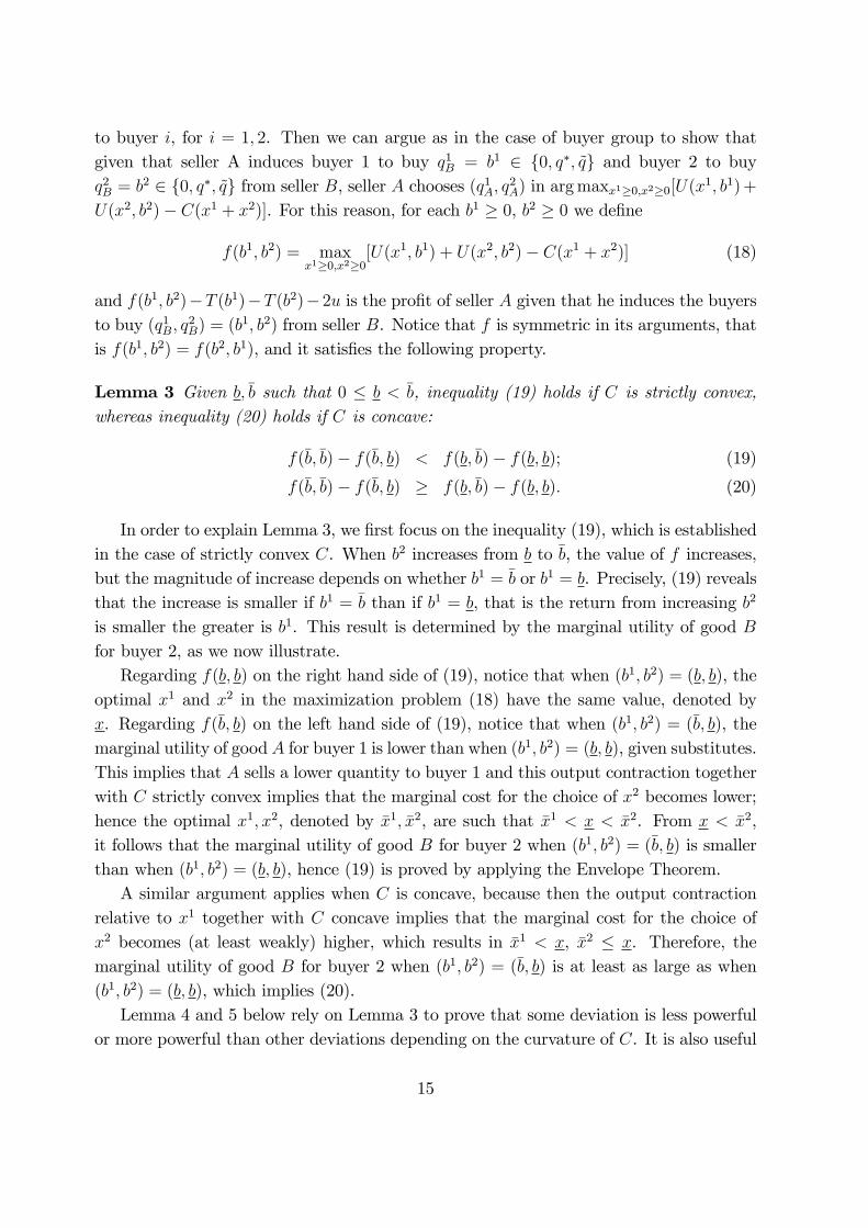
U(x2, b2)− C(x1 + x2)]. For this reason, for each b1 ≥ 0, b2 ≥ 0 we define

f(b1, b2) = maxx1≥0,x2≥0

[U(x1, b1) + U(x2, b2)− C(x1 + x2)] (18)

and f(b1, b2)−T (b1)−T (b2)−2u is the profit of seller A given that he induces the buyersto buy (q1B, q

2B) = (b1, b2) from seller B. Notice that f is symmetric in its arguments, that

is f(b1, b2) = f(b2, b1), and it satisfies the following property.

Lemma 3 Given b, b such that 0 ≤ b < b, inequality (19) holds if C is strictly convex,whereas inequality (20) holds if C is concave:

f(b, b)− f(b, b) < f(b, b)− f(b, b); (19)

f(b, b)− f(b, b) ≥ f(b, b)− f(b, b). (20)

In order to explain Lemma 3, we first focus on the inequality (19), which is establishedin the case of strictly convex C. When b2 increases from b to b, the value of f increases,but the magnitude of increase depends on whether b1 = b or b1 = b. Precisely, (19) revealsthat the increase is smaller if b1 = b than if b1 = b, that is the return from increasing b2

is smaller the greater is b1. This result is determined by the marginal utility of good Bfor buyer 2, as we now illustrate.Regarding f(b, b) on the right hand side of (19), notice that when (b1, b2) = (b, b), the

optimal x1 and x2 in the maximization problem (18) have the same value, denoted byx. Regarding f(b, b) on the left hand side of (19), notice that when (b1, b2) = (b, b), themarginal utility of good A for buyer 1 is lower than when (b1, b2) = (b, b), given substitutes.This implies that A sells a lower quantity to buyer 1 and this output contraction togetherwith C strictly convex implies that the marginal cost for the choice of x2 becomes lower;hence the optimal x1, x2, denoted by x1, x2, are such that x1 < x < x2. From x < x2,it follows that the marginal utility of good B for buyer 2 when (b1, b2) = (b, b) is smallerthan when (b1, b2) = (b, b), hence (19) is proved by applying the Envelope Theorem.A similar argument applies when C is concave, because then the output contraction

relative to x1 together with C concave implies that the marginal cost for the choice ofx2 becomes (at least weakly) higher, which results in x1 < x, x2 ≤ x. Therefore, themarginal utility of good B for buyer 2 when (b1, b2) = (b, b) is at least as large as when(b1, b2) = (b, b), which implies (20).Lemma 4 and 5 below rely on Lemma 3 to prove that some deviation is less powerful

or more powerful than other deviations depending on the curvature of C. It is also useful

15

to know that (19) is equivalent to

f(b, b)− f(b, b) < 2[f(b, b)− f(b, b)

];

and (20) is equivalent to

f(b, b)− f(b, b) ≥ 2[f(b, b)− f(b, b)

].

Given u, each seller’s profit is 2t∗ −C(2q∗), which is equal to f(q∗, q∗)−U(q∗, q∗)− u[from (17) and (18)]. In equilibrium, this profit should be higher than any deviationprofit. Let (IC (b1, b2)) represent the incentive constraint that makes it unprofitable forseller j (= A,B) to deviate by inducing the buyers to buy (q1k, q

2k) = (b1, b2) from seller k

(= A,B) with j 6= k, b1 ∈ {0, q∗, q}, b2 ∈ {0, q∗, q} and (b1, b2) 6= (q∗, q∗):

(IC(b1, b2

)) f(q∗, q∗)− U(q∗, q∗)− u ≥ f(b1, b2)− T (b1)− T (b2)− 2u.

We start by considering two deviations that determine a lower bound of u. First, thedeviation which induces both buyers to buy exclusively from seller j yields a profit off(0, 0) − 2u. Therefore, f(q∗, q∗) − U(q∗, q∗) − u ≥ f(0, 0) − 2u must be satisfied, whichis equivalent to

(IC (0, 0)) f(0, 0)− f(q∗, q∗) + U(q∗, q∗) ≤ u. (21)

Second, the deviation which induces one buyer to buy exclusively from j and theother buyer to buy q∗ from k yields j a profit of f(0, q∗)− 2u− t∗. Therefore, f(q∗, q∗)−U(q∗, q∗)− u ≥ f(0, q∗)− 2u− t∗ must be satisfied, which is equivalent to

(IC (0, q∗)) 2f(0, q∗)− 2f(q∗, q∗) + U(q∗, q∗) ≤ u. (22)

The second deviation involves a discriminatory offer, and now we inquire when thisstrategy has a bite, in the sense that it is stronger than the deviation inducing both buyersto buy exclusively from j. To this purpose, we use Lemma 3 with b = 0 < b = q∗:

Lemma 4 Consider the symmetric setting without buyer group.(i) Suppose that C is strictly convex. Then, if (IC (0, q∗)) is satisfied, (IC (0, 0)) is

satisfied as well: f(q∗, q∗)− f(0, 0) < 2 [f(0, q∗)− f(0, 0)]

(ii) Suppose that C is concave. Then, if (IC (0, 0)) is satisfied, (IC (0, q∗)) is satisfiedas well: f(q∗, q∗)− f(0, 0) ≥ 2 [f(0, q∗)− f(0, 0)].

Let us consider seller A’s deviations. Both deviations we are focusing on require sellerA to produce more output than without the deviations but the deviation which inducesboth buyers to make exclusive purchases from A requires a greater increase in outputthan the other deviation. When costs are convex (concave), marginal cost is increasing

16

(decreasing) and hence inducing a first buyer to buy exclusively involves a smaller (larger)increase in cost per output than inducing a second buyer to buy exclusively. Therefore,when costs are strictly convex, inducing both buyers to make exclusive purchases is notprofitable if inducing only one buyer to make exclusive purchase is not profitable. Sym-metrically, when costs are concave, inducing only one buyer to make exclusive purchaseis not profitable if inducing both buyers to make exclusive purchase is not profitable.Lemma 4 implies the following lower bound on u depending on whether C is convex

or concave:

2f(0, q∗)− 2f(q∗, q∗) + U(q∗, q∗) ≤ u if C is strictly convex;f(0, 0)− f(q∗, q∗) + U(q∗, q∗) ≤ u if C is concave.

(23)

Now we consider two different deviations which generate an upper bound for u. First,the deviation which induces buyer 1 to buy q∗ and buyer 2 to buy q(> q∗) from B

yields seller A the profit f(q∗, q) − t∗ − t − 2u. Therefore, f(q∗, q∗) − U(q∗, q∗) − u ≥f(q∗, q)− t∗ − t− 2u must be satisfied, which is equivalent to

(IC (q∗, q)) u ≤ 2f(q∗, q∗)− U(q∗, q∗)− 2[f(q∗, q)− U(0, q)].

Second, the deviation which induces each buyer to buy q from B yields seller A profitf(q, q)− 2t− 2u. Therefore, f(q∗, q∗)−U(q∗, q∗)−u ≥ f(q, q)− 2t− 2u must be satisfied,which is equivalent to

(IC (q, q)) u ≤ f(q∗, q∗)− U(q∗, q∗)− [f(q, q)− 2U(0, q)].

In order to inquire which deviation is stronger, we use again Lemma 3, this time withb = q∗ < b = q:

Lemma 5 Consider the symmetric setting without buyer group.(i) Suppose that C is strictly convex. Then, if (IC (q∗, q)) is satisfied, (IC (q, q)) is

satisfied as well: f(q, q)− f(q∗, q∗) < 2 [f(q∗, q)− f(q∗, q∗)].(ii) Suppose that C is concave. Then, if (IC (q, q)) is satisfied, (IC (q∗, q)) is satisfied

as well: f(q, q)− f(q∗, q∗) ≥ 2 [f(q∗, q)− f(q∗, q∗)].

Both deviations we are considering require seller A to produce less output than withoutthe deviations, and the deviation which induces each buyer to buy quantity q from sellerB is the deviation involving a higher reduction in output than the other deviation. Whencosts are convex (concave), the marginal saving in cost from output contraction decreases(increases) as the amount of output reduction increases. Therefore, when costs are convex,the deviation inducing (q1B, q

2B) = (q, q) generates a lower saving per reduced output than

the deviation inducing (q1B, q2B) = (q∗, q), which implies that if the latter deviation is

17

unprofitable, then the former deviation is unprofitable as well. A symmetric argumentapplies when costs are concave, which implies that if the deviation inducing (q1B, q

2B) =

(q, q) is unprofitable, the deviation inducing (q1B, q2B) = (q∗, q) is unprofitable.

Lemma 5 implies the following upper bound on u depending on whether C is convexor concave:

u ≤ 2f(q∗, q∗)− U(q∗, q∗)− 2[f(q∗, q)− U(0, q)] if C is strictly convex;u ≤ f(q∗, q∗)− U(q∗, q∗)− [f(q, q)− 2U(0, q)] if C is concave.

(24)

From (23) and (24) we derive an interval of values for u which depends on the curvatureof C. In fact, before we can conclude that this interval is the set of equilibrium valuesfor each buyer’s payoff, we need to verify that, given

(t∗, t)satisfying (17), each buyer

wants to buy quantity q∗ from each seller and we must establish the unprofitability of anydeviation of each seller. The proof of the next proposition takes care of these issues and,in addition, establishes that each of the two right hand sides in (24) is increasing in q.

Proposition 3 (Equilibrium without buyer group) Consider the symmetric setting with-out buyer group.(a) Suppose that C is strictly convex. There exists a symmetric equilibrium in which

each buyer’s payoff is u if and only if

U(q∗, q∗)− 2f(q∗, q∗) + 2f(0, q∗) ≤ u ≤ 2f(q∗, q∗)− U(q∗, q∗)− 2 limb→+∞

[f(q∗, b)− U(0, b)]

(25)(b) Suppose that C is concave. There exists a symmetric equilibrium in which each buyer’spayoff is u if and only if

f(0, 0)− f(q∗, q∗) + U(q∗, q∗) ≤ u ≤ f(q∗, q∗)− U(q∗, q∗)− limb→+∞

[f(b, b)− 2U(0, b)] (26)

Example Consider again the example of U(qA, qB) = (q1/2A + q

1/2B )1/2 and C(q) = 1

2q2,

with U(q∗, q∗) = 1, C(2q∗) = 18. Since C is strictly convex, the interval of values for u is

(25). Since f(q∗, q∗) = 158and f(0, q∗) = maxx≥0,y≥0[x

1/4 + (y1/2 + 12)1/2 − 1

2(x + y)2] =

1.5913, the lower bound for u is 0.4326.Regarding the upper bound for u, we find that

f(q∗, b)− U(0, b) = maxx≥0,y≥0

[(x1/2 +1

2)1/2 + (y1/2 + b1/2)1/2 − 1

2(x+ y)2 − b1/4]

= maxx≥0,y≥0

[(x1/2 +1

2)1/2 − 1

2(x+ y)2 +

y1/2

(y1/2 + b1/2)1/2 + b1/4] (27)

and limb→+∞ (f(q∗, b)− U(0, b)) = maxx≥0[(x1/2 + 1

2)1/2 − 1

2x2] = 0.98442.

Hence the interval for u is[0.4326, 0.78116)

18

5 Comparison between buyer group and no group

In this section, we still consider the symmetric setting and compare the equilibria underbuyer group and those without group. In the case of buyer group, if uG is the group’s payoffthen each buyer’s payoff is uG/2, hence the bounds in (12) below for the case of groupcan be expressed in terms of u as in (28), where we exploit the equalities fG(0) = f(0, 0)

and limb→+∞[fG(b)− UG(0, b)] = limb→+∞[f(b, b)− 2U(0, b)]

f(0, 0)− 1

2V GAB ≤ u ≤ 1

2V GAB − lim

b→+∞[f(b, b)− 2U(0, b)] (28)

Since 12V GAB = U(q∗, q∗)−C(2q∗) = f(q∗, q∗)−U(q∗, q∗), we see that the interval of payoff

in (28) is the same as the interval for no group we previously identified in (26). Therefore,when C is concave (which includes the case of linear C), the set of equilibrium outcomesis unaffected by group formation. Matters are different when C is strictly convex, as nextproposition establishes

Proposition 4 Consider the symmetric setting.(a) If C is concave, then the interval of equilibrium payoffs for each buyer is the same

regardless of whether or not buyers form a group.(b) If C is strictly convex, then the interval of equilibrium payoffs for each buyer under

no group is a strict subset of the interval of equilibrium payoffs for each buyer under buyergroup. Formally,

f(0, 0)− 1

2V GAB < U(q∗, q∗)− 2f(q∗, q∗) + 2f(0, q∗) (29)

2f(q∗, q∗)−U(q∗, q∗)− 2 limb→+∞

[f(q∗, b)−U(0, b)] <1

2V GAB − lim

b→+∞[f(b, b)− 2U(0, b)] (30)

Buyer group has no effect on the interval of the equilibrium payoffs for the buyerswhen C is concave, but if C is strictly convex, from the buyers’point of view, the payoffof the worst equilibrium without group is higher than the payoff of the worst equilibriumunder buyer group, while the payoff of the best equilibrium without group is lower thanthe payoff of the best equilibrium under buyer group.In order to see why these differences arise, recall from Section 3 that the lower bound

for uG is determined by seller A’s deviation with qGB = 0, which is equivalent to thedeviation of seller A under no group with q1B = 0, q2B = 0. The latter deviation implies2u + πA ≥ f(0, 0) in any equilibrium, hence πB ≤ V G

AB − f(0, 0). But under no group,seller A can also deviate with q1B = 0, q2B = q∗. This generates a total payoff for buyersand seller A equal to f(0, q∗)−t∗, hence 2u+πA ≥ f(0, q∗)−t∗. When u = f(0, 0)− 1

2V GAB,

we find that f(0, 0) ≥ f(0, q∗)−t∗ if C is concave, but f(0, q∗)−t∗ > f(0, 0) if C is strictly

19

convex. Therefore, for concave C the lower bound in (26) is determined by the deviationwhich induces both buyers to make exclusive purchase from the deviating seller, as underbuyer group. Conversely, when C is strictly convex the inequality f(0, q∗) − t∗ > f(0, 0)

implies for πB (and for πA) that πB ≤ V GAB − (f(0, q∗)− t∗) < V G

AB − f(0, 0), therefore thelower bound in (25) is greater than the lower bound in (28), as (29) establishes.In Section 3 we have also explained that under buyer group, the best equilibrium

for buyers is determined by seller A’s deviation with qGB = q (for q → +∞). This isanalogous to seller A’s deviation under no group with q1B = q, q2B = q (for q → +∞)which yields seller A the profit f(q, q) − 2t − 2u. But under no group, seller A canalso deviate with q1B = q, q2B = q∗, which yields A the profit f(q, q∗)− t− t∗ − 2u. Whenu = 1

2V GAB−[f(q, q)−2U(0, q)], we have f(q, q)−2t−2u ≥ f(q, q∗)−t−t∗−2u if C is concave,

but f(q, q)−2t−2u < f(q, q∗)− t−t∗−2u if C is strictly convex. Therefore, for concave Cthe upper bound in (26) is determined by the deviation which induces each buyer to buyfrom the non-deviating seller a quantity higher than the equilibrium quantity, just like inthe deviation which identifies the upper bound in (28) under buyer group. Conversely,when C is strictly convex the inequality f(q, q)− 2t− 2u < f(q, q∗)− t− t∗− 2u increasesthe lower bound for πA, hence decreases the upper bound for u as (30) establishes.As we remarked in Section 4, the difference between buyer group and no group lies

in the possibility for sellers to use discriminatory offers when there is no group. Butwhen C is concave that has no effect as the deviations that determine the bounds for theequilibrium payoffs do not involve discriminatory offers. Conversely, when C is strictlyconvex, discriminatory offers have multiple effects: (i) they intensify competition betweensellers at their most favorable equilibrium, thus increasing u in the worst equilibrium forbuyers; (ii) they make more effective the deviation which determines the sellers’lowestequilibrium profit, thus reducing the buyers’highest payoff. As a result, under no buyergroup the bounds for u are tighter. Notice that if discriminatory offers were infeasible,then the interval of equilibrium payoffs for each buyer would be given by (28), that is(26), even when C is strictly convex.28

Example Consider the example of U(qA, qB) = (q1/2A +q

1/2B )1/2 and C(q) = 1

2q2. Under

the buyer group, uG/2 belongs to [0.4252, 0.875), whereas without buyer group, u belongsto [0.4326, 0.78116). Consistently with Proposition 4(b), given that C is strictly convex,buyer group reduces the lower bound of each buyer’s payoffand increases the upper bound.

28Our results depend on the assumption that good are strict substitutes. If instead products haveindependent values (i.e., there exists a U : [0,+∞)→ R such that U(qA, qB) = U(qA) + U(qB)), then thelower and upper bounds in (25), (26), (28) are all equal to 0, independently of the curvature of C. Thisoccurs because each seller can act like a perfectly discriminating monopolist, as each buyer’s valuationfor seller j’s product does not depend on the quantity the buyer buys from the other seller. Therefore,seller j can fully extract each buyer’s surplus regardless of whether or not buyers form a group.

20

In terms of the percentage with respect to the payoffwithout group, buyer group reducesthe lower bound by 1.7 percent and increases the upper bound by 12 percent.

Remark The multiplicity of equilibria, both with and without buyer group, makes itnot straightforward to derive clear predictions about the effect of forming a buyer group.When C is concave, buyer group has no effect on the set of equilibrium payoffs and hencewe can say that buyer group has no effect no matter the equilibrium selection. WhenC is strictly convex, we notice that one natural and widely applied selection rule amongmultiple equilibria is the one which focuses on Pareto optimal equilibria for the players.In the game which starts at stage one (after either decision of the buyers about groupformation at stage zero), the players are sellers A and B, and both in the case of groupformation and of no group, there exists a unique Pareto optimal equilibrium for sellers.This is the equilibrium which corresponds to the lowest uG in (12), and to the lowest uin (25). Under the Pareto optimal equilibrium selection rule, Proposition 4 implies thatforming a group is harmful for buyers because of (29). In fact, when C is strictly convex,this prediction holds as long as the Pareto-dominant equilibrium is selected under buyergroup, no matter the equilibrium selected without buyer group.

6 Extension to a general setting

In this section, we extend a main result from the symmetric setting to a general settingwith two asymmetric sellers and n ≥ 2 asymmetric buyers. Namely, we extend the resultin Proposition 4(b) that buyer group reduces the worst payoff of the buyers when sellers’cost functions are strictly convex. In the generalization, we compare the payoffs withoutbuyer group with the payoffs in the sell-out equilibrium under buyer group, which is thePareto-dominant equilibrium for sellers. We show that every equilibrium without groupyields the buyers a strictly higher total payoff (and each seller a strictly lower payoff)than the payoff in the sell-out equilibrium under buyer group.

Proposition 5 Suppose that there are n ≥ 2 buyers (with no assumption of symmetryfor buyers, nor for sellers), and the cost function of at least one seller is strictly convex.Then, in any equilibrium without buyer group, the buyers obtain a strictly higher totalpayoff (and each seller obtains a strictly lower payoff ) than in the sell-out equilibriumunder buyer group.

The proof of Proposition 5 relies on the following generalization of (19) in Lemma 3to n ≥ 2 asymmetric buyers and two asymmetric sellers, which is proved in the proof ofLemma 3 in Appendix. Let us consider seller A for instance. Given b1 ≥ 0, b2 ≥ 0, ...,bn ≥ 0, fA(b1, b2, ..., bn) is defined as maxx1,x2,...,xn [U1(x1, b1)+U2(x2, b2)+...+Un(xn, bn)−

21

CA(x1+x2+ ...+xn)]. Then, given b1, ..., bn and b1, ..., bn such that bh < bh for h = 1, ..., n,we prove that

fA(b1, ..., bn)− fA(b1, ..., bn) <

n∑i=1

[fA(b1, ..., bi, ..., bn)− fA(b1, ..., bn)

]if CA is strictly convex. This generalizes the inequality f(b, b)−f(b, b) < 2

[f(b, b)− f(b, b)

]in Section 4.

7 Application: entry and buyer group

In this section, we use our main insight to study how the possibility of a seller’s entryaffects the buyers’decision to form a group. For instance, a buying alliance among largechains of supermarkets can have an impact on the entry of national brand manufacturers.29

Innes and Sexton (1993, 1994) allow the possibility for the buyers to form a coalitionin order to contract with an outside entrant (or vertically integrate into the upstreammarket). In their papers, the incumbent has the first mover advantage and employsdivide-and-conquer strategies to disrupt the coalition building. In contrast, we assumethat the buyers move first by deciding whether to form or not a group and also assume thatthe incumbent and the entrant compete by making simultaneous offers as in Fumagalliand Motta (2008).30

We consider a setting with an incumbent, seller A, and a potential entrant, seller B,assuming that the cost functions are strictly convex and the products are strict substitutes.The buyers decide whether to form a group or not before the realization of the fixed costof entry f of seller B. Let V G

j ≡ maxx≥0[UG(x, 0)− Cj(x)] denote the welfare generated

when the group trades only with seller j (= A,B). We assume that f is distributed over[0, f]with f > V G

AB − V GA (> 0) with a cumulative distribution function H with a strictly

positive density h in[0, f]. We study the following game:

• Stage 0: The buyers decide whether or not to form a group.

• Stage 0.5: The fixed cost of entry f ≥ 0 of the entrant is realized. The entrantdecides whether to incur the cost or not.

29Caprice and Rey (2015) describe the buying alliance between Leclerc and Système U, each having17% and 9% of sales in French grocery and daily goods retail markets in 2009.30Fumagalli and Motta (2008) assume that the entrant can make his offer before incurring a fixed cost

of entry, which seems less natural than our timing that the entrant makes an offer after incurring theentry cost.

22

• Stage 1: If the entrant entered, then the incumbent and the entrant compete bysimultaneously proposing non-linear tariffs to each buyer (or to the buyer group).If the entrant did not enter, the incumbent becomes monopolist.

• Stage 2: Each buyer i, or the buyer group, makes purchase decisions.

If the entrant enters, given the multiplicity of equilibria, we select the equilibriumwhich is Pareto-dominant in terms of the sellers’ payoffs. Hence, the sellers play thesell-out equilibrium under buyer group and the sellers’payoffs are V G

AB − V GB for seller A,

V GAB−V G

A for seller B (Bernheim andWhinston, 1998). The assumption VGAB−V G

A ∈ (0, f)

implies that when the buyer group is formed, seller B enters with a positive probabilityH(V G

AB − V GA ) ∈ (0, 1). Proposition 5 suggests that the buyers face a clear trade-off.

Conditional on entry, the total payoff of the buyers is lower under buyer group thanunder no group. However, the fact that the entrant’s payoff is higher under buyer groupthan without group makes the probability of entry higher under buyer group than underno group. Furthermore, in the sell-out equilibrium under buyer group, each seller obtainsthe social incremental contribution of his product, implying that the entry decision isalways socially optimal. This in turn suggests that if buyers remain separate, then theentry is suboptimal. Therefore, Proposition 5 suggests that the buyers may deliberatelyinduce a suboptimal entry by remaining separate in order to benefit from more intensecompetition upon entry.

Proposition 6 (entry) Suppose that the cost functions are strictly convex and the prod-ucts are strict substitutes. Consider the game of buyer group formation followed by theentry. In case the entrant enters, we select the equilibrium which is Pareto-dominant interms of the sellers’payoffs.(i) If the buyers form a group, then the private entry decision is socially effi cient. But

if the buyers remain separate, then the entry is suboptimal.(ii) The buyers may deliberately induce a suboptimal entry by remaining separate in

order to benefit from more intense competition upon entry.

The existing literature on naked exclusion explains suboptimal entry by the incum-bent’s taking advantage of coordination failure among buyers (Rasmusen, Ramseyer andWiley 1991, Segal and Whinston, 2000, Fumagalli and Motta, 2006, 2008, Chen andShaffer, 2014). While the literature typically assumes that the incumbent makes offers tobuyers before the entry, Fumagalli and Motta (2008) show that the coordination failuresurvives even if both sellers make simultaneous offers. However, in these papers, buyershave no reason not to form a group (at least among those operating in separate markets)as this would remove the coordination failure. We show that buyers may choose not toform a group even if this leads to a suboptimal entry.

23

8 Linear costs with both complements and substi-tutes

In this section, we consider a setting with linear costs, but we relax the assumption ofsubstitute goods and assume that goods are complements for at least one buyer. We dis-cover another mechanism which makes buyers lose from building a group, and is differentfrom the one identified previously based on strictly convex costs.Given linear cost functions, with constant marginal cost cj for each seller j, there

exists sell-out equilibria both if the buyers form a group and if they remain separate. Inwhat follows, we focus on this class of equilibria. More precisely, in the case of no group,let V i

AB ≡ U i (qi∗A , qi∗B )−cAqi∗A −cBqi∗B denote the welfare generated when buyer i purchases

(qi∗A , qi∗B ) from both sellers. Let V i

j ≡ maxqij [Ui(qij, 0)− cjqij] denote the welfare generated

when buyer i trades only with seller j. If the two products are substitutes for buyer i,then it is necessary that V i

AB−F iA−F iB = V iA−F iA = V i

B−F iB in the sell-out equilibrium.From these equalities we obtain the unique equilibrium fees:

F i∗A = V iAB − V i

B, F i∗B = V iAB − V i

A, for i = 1, 2. (31)

and the payoff of buyer i is V iA + V i

B − V iAB ≥ 0.

Suppose now that products are complements for buyer 2. This implies V 2A+V 2

B < V 2AB,

hence the payoff of buyer 2 is negative if the fixed fees are given as in (31). As the payoffcannot be negative, the equilibrium fixed fees must be lower than in (31), but in factthere exist infinitely many equilibrium fixed fees: they are such that F 2A + F 2B = V 2

AB

and V 2A ≤ F 2A, V

2B ≤ F 2B.

31 The first equality implies that buyer 2’s payoff is zero. Themultiplicity is about how the sellers share the surplus of V 2

AB − V 2A − V 2

B generated bycomplementarity between the two products, but this is not very relevant for us, as inevery equilibrium buyer 2’s payoff is zero.Linear costs imply V G

AB = V 1AB+V 2

AB and VGA = V 1

A+V 2A, V

GB = V 1

B+V 2B, where we recall

that V GA for instance represents the welfare generated when the group trades only with

seller A. Therefore, if products are complements for each buyer, that is if V 1A + V 1

B ≤ V 1AB

and V 2A + V 2

B ≤ V 2AB, then both buyers have zero payoff under no group, and also the

group has zero payoff since V GA + V G

B ≤ V GAB. Buyer group has no effect in this case.

Suppose now that the products are strict substitutes for buyer 1 and strict comple-ments for buyer 2: V 1

A +V 1B > V 1

AB and V2A +V 2

B < V 2AB. Then, if the group is not formed,

the sum of the buyers’payoffs coincides with the payoff of buyer 1, which is equal toV 1A + V 1

B − V 1AB > 0. If the group is formed, then its payoff is given by

max{

0, V 1A + V 1

B + V 2A + V 2

B − V 1AB − V 2

AB

},

31These inequalities imply F 2A ≤ V 2AB − V 2B and F 2B ≤ V 2AB − V 2A.

24

which is always strictly less than V 1A+V 1

B−V 1AB because V

2A+V 2

B < V 2AB. Therefore, in this

case the group strictly reduces the sum of the payoffs of the buyers. The intuition is prettysimple. When the products are complements for buyer 2, each seller j has some residualmarket power with respect to buyer 2 in the sense that because of the constraint thatbuyer 2’s payoff cannot be negative, seller j charges less than the marginal value createdby his product. Integrating the two markets through buyer group allows the sellers totransfer their residual market power to the market of buyer 1. This mechanism is similarto the mechanism through which multi-market contact facilitates collusion by transferringresidual collusive power from one market to another (Bernheim and Whinston, 1990).

Proposition 7 (complements and substitutes) Assume linear cost functions. Then theformation of the buyer group(i) has no effect on any player’s payoff if the products are complements to both buyers;(ii) strictly reduces the joint payoff of the buyers if the products are strict complementsfor one buyer but strict substitutes for the other.

9 Conclusion

We considered buyer group which cannot pre-commit to exclusive purchase and foundthat buyer group does not generate buyer power (i.e., larger discounts than no buyergroup), no matter the curvature of the sellers’cost function. Combining our result withthose of Inderst and Shaffer (2007) and Dana (2012) generates a clear message: whenmultiple sellers producing substitutes compete, buyer group creates buyer power only ifthe group can pre-commit to limit its purchase to a subset of sellers. This has policyimplications, for instance, to large healthcare procurement alliances. It is not the meresize of the alliance, but the credible threat to limit its purchase to a subset of sellers whichincreases its buyer power.It would be interesting to extend our framework by considering a linear contract be-

tween an upstream firm and a downstream firm instead of a non-linear contract. Thelinear contract is prominent in relations between TV channels and cable TV distribu-tors (Crawford and Yurukoglu, 2012), between hospitals and medical device suppliers(Grennan, 2013, 2014), and between book publishers and resellers (Gilbert, 2015). Withsuch simple but realistic contract, the equilibrium outcome is in general ineffi cient sinceeach upstream firm adds a positive markup. Therefore, if buyer fragmentation intensifiescompetition between sellers as in this paper, it will increase welfare by reducing the dead-weight loss. In addition, the framework with the linear contract may be tractable enoughto incorporate competition among downstream firms.

25

10 Acknowledgements

We thank one anonymous advisory editor and two anonymous referees, Stéphane Caprice,Zhijun Chen, Jay Pil Choi, Vincenzo Denicolo, Biung-Ghi Ju, Bruno Jullien, In-UckPark, Patrick Rey and the audience who attended our presentations at Bristol University,EARIE (2014), EEA-ESEM (2014), Postal Economics Conference on "E-commerce, Digi-tal Economy and Delivery Services" (Toulouse, 2014), Seoul National University, ToulouseSchool of Economics, Yonsei University.This research did not receive any specific grant from funding agencies in the public,

commercial, or not-for-profit sectors.

References

[1] Aghion, Philippe and Bolton, Patrick (1987). “Contracts as a Barrier to Entry.”American Economic Review, 77(3): 388—401.

[2] Bernheim, Douglas and Michael Whinston (1986). “Menu Auctions, Resource Allo-cation and Economic Influence.”Quarterly Journal of Economics, 101, 1-31.

[3] Bernheim, Douglas and Michael Whinston (1990). ”Multi-market Contact and Col-lusive Behavior.”The RAND Journal of Economics, 21(1), 1-26.

[4] Bernheim, Douglas and Michael Whinston (1998). “Exclusive Dealing.”Journal ofPolitical Economy, 106, 64-103.

[5] Caprice, Stéphane and Patrick Rey (2015). "Buyer Power From Joint Listing Deci-sions." Economic Journal,125: 1677-1704

[6] Chae, Suchan and Paul Heidhues (2004). "Buyers’Alliances for Bargaining Power."Journal of Economics and Management Strategy, 13: 731—754

[7] Chen, Yuxin and Xinxin Li (2013). "Group Buying Commitment and Sellers’Com-petitive Advantages", Journal of Economics and Management Strategy, 22:164-183.

[8] Chen, Zhijun and Greg Shaffer (2014). "Naked Exclusion with Minimum-Share Re-quirements", RAND Journal of Economics, 45: 64-91.

[9] Chen, Zhiqi, (2003). "Dominant Retailers and Countervailing Power Hypothesis",RAND Journal of Economics, 34: 612-625.

[10] Chen, Zhiqi (2007). "Buyer Power: Economic Theory and Antitrust Policy", Researchin Law and Economics 22:17-40.

26

[11] Chipty, T. and Snyder, C.M. (1999). "The Role of Firm Size in Bilateral Bargaining:a Study of the Cable Television Industry", Review of Economics and Statistics, 81:326-40.

[12] Competition Commission (2008). The Supply of Groceries in the UK Market Inves-tigation, U.K. Competition Commission, London

[13] Crawford, Gregory S., and Ali Yurukoglu (2012). “The Welfare Effects of Bundlingin Multichannel Television Markets.”American Economic Review, 102: 643—685

[14] Dana, James D. (2012). "Buyer Group as Strategic Commitments", Games and Eco-nomic Behavior, 74(2): 470-485.

[15] DeGraba, Patrick J. (2005). "Quantity Discounts from Risk Averse Sellers," U. S.Federal Trade Commission Working Paper no. 276.

[16] Dobson, Paul W. and Michael Waterson, (1997). "Countervailing Power and Con-sumer Prices," Economic Journal, 107: 418—430.

[17] Ellison, Sara Fisher and Christopher M. Snyder (2010). "Countervailing Power inWholesale Pharmaceuticals", Journal of Industrial Economics, 58: 32-53.

[18] Erutku, Can, (2005). "Buying Power and Strategic Interactions," Canadian Journalof Economics, 38: 1160—1172.

[19] European Commission (1999). Buyer power and his impact on competition in the foodretail distribution sector of the European Union: Final report.

[20] Fumagalli, Chiara and Massimo Motta (2006). "Exclusive Dealing and Entry, WhenBuyers Compete," American Economic Review, 96: 785-944.

[21] Fumagalli, Chiara and Massimo Motta (2008). "Buyers’Miscoordination, Entry andDownstream Competition," Economic Journal, 118: 1196-1222.

[22] Gaudin, Germain (2017). "Vertical Bargaining and Retail Competition: What DrivesCountervailing Power?" Economic Journal, forthcoming

[23] Gilbert, Richard J. (2015). “E-Books: A Tale of Digital Disruption.” Journal ofEconomic Perspectives, 29: 165—184.

[24] Grennan, Matthew (2013). “Price Discrimination and Bargaining: Empirical Evi-dence from Medical Devices.”American Economic Review, 103: 145—177.

27

[25] Grennan, Matthew (2014). “Bargaining Ability and Competitive Advantage: Empir-ical Evidence from Medical Devices.”Management Science, 60: 3011—3025.

[26] Harsanyi, J. C. (1977). Rational Behavior and Bargaining Equilibrium in Games andSocial Situations. Cambridge: Cambridge University Press.

[27] Inderst, R and G. Shaffer (2007). "Retail Mergers, Buyer Power and Product Vari-ety", The Economic Journal, 117(516): 45-67.

[28] Inderst, R. and Tommaso Valletti (2011). "Buyer Power and the ‘Waterbed effect’",Journal of Industrial Economics 59: 1-20

[29] Inderst, R and C. Wey (2003). "Bargaining, Mergers, and Technology Choice inBilaterally Oligopolistic Industries", the RAND Journal of Economics, 34: 1-19.

[30] Inderst, R and C. Wey (2007). "Buyer Power and Supplier Incentives", EuropeanEconomic Review, 51: 647-667.

[31] Innes, R. and R. J. Sexton (1993). ”Customer Coalitions, Monopoly Price Discrimi-nation and Generic Entry Deterrence.”European Economic Review, 37, 1569-1597.

[32] Innes, R. and R. J. Sexton (1994). ”Strategic Buyers and Exclusionary Contracts”,American Economic Review, 84: 566-584.

[33] Jeon, Doh-Shin and Domenico Menicucci (2005). “Optimal Second-Degree Price Dis-crimination and Arbitrage: On the Role of Asymmetric Information among Buyers”,The RAND Journal of Economics, 36 (2), pp. 337-360.

[34] Jeon, Doh-Shin and Domenico Menicucci (2006). “Bundling Electronic Journals andCompetition among Publishers”, Journal of the European Economic Association,September 4(5): 1038-83.

[35] Jeon, Doh-Shin and Domenico Menicucci (2012). “Bundling and Competition forSlots”, American Economic Review, 102: 1957-1985.

[36] Jeon, Doh-Shin and Domenico Menicucci (2017). “The Benefits of Diverse Preferencesin Library Consortia," Journal of Industrial Economics 65: 105-135

[37] Katz, Michael (1987). "The Welfare Effects of Third Degree Price Discrimination inIntermediate Goods Markets," American Economic Review, 77: 154—167.

[38] Loertscher, Simon and Leslie M. Marx (2017). "Merger Reviews for Markets withBuyer Power," Mimeo

28

[39] Marvel, H.P. and H. Yang, (2008). "Group Purchasing, Nonlinear Tariffs, andOligopoly," International Journal of Industrial Organization, 26(5): 1090-1105.

[40] Normann, H.-T., Ruffl e, B. and Snyder, C. M., (2007). "Do Buyer-Size DiscountsDepend on the Curvature of the Surplus Function? Experimental Tests of BargainingModels," , Rand Journal of Economics, 38: 747—767.

[41] O’Brien, Daniel and Greg Shaffer (1997). "Non-linear Supply Contracts, ExclusiveDealing and Equilibrium Market Foreclosure", Journal of Economics and Manage-ment Strategy 6: 755-785

[42] OECD (2008). Monopsony and Buyer Power, Policy Roundtables.

[43] Prat, Andrea and Aldo Rustichini (2003). "Games Played through Agents", Econo-metrica, 71 (4): 989-1026

[44] Rasmusen, Eric B., J. Mark Ramseyer, and John S. Wiley, Jr. (1991). “Naked Ex-clusion.”American Economic Review, 81(5): 1137—45.

[45] Ruffl e, Bradley J. (2013). "When Do Large Buyers Pay Less? Experimental Evi-dence", Journal of Industrial Economics 61: 108-137

[46] Scheffman, David. T. and Pablo T. Spiller (1992). "Buyers’Strategies, Entry Barriersand Competition," Economic Inquiry, 30: 418—436

[47] Segal, Ilya and Michael Whinston (2000). "Naked Exclusion: Comment", AmericanEconomic Review, 190: 296-309

[48] Snyder, Christopher M., (1996). "A Dynamic Theory of Countervailing Power," RandJournal of Economics, 27: 747—769.

[49] Snyder, Christopher M., (1998). "Why Do Larger Buyers Pay Lower Prices? IntenseSupplier Competition," Economics Letters, 58: 205—209.

[50] Sorensen, Alan T., (2003). "Insurer-Hospital Bargaining: Negotiated Discounts inPost-Deregulation Connecticut," Journal of Industrial Economics, 51: 471—492.

[51] van den Brink, R. (2012), “Effi ciency and Collusion Neutrality in Cooperative Gamesand Networks”, Games and Economic Behavior, 76, 344-348.

[52] von Ungern-Sternberg, T. (1996). "Countervailing Power Revisited", InternationalJournal of Industrial Organization, 14: 507-19.

29

11 Appendix

11.1 Proof of Proposition 1

The case of buyer group Here we only prove that UG is concave, since the rest of theproof is in the main text.Consider (qGA , q

GB) = (qA, qB), and suppose that (q1A, q

1B, q

2A, q

2B) is the optimal allo-

cation (i.e., it maximizes G’s payoff32) given (qGA , qGB) = (qA, qB), that is UG(qA, qB) =

U1(q1A, q1B)+U2(q2A, q

2B). Likewise, consider (qGA , q

GB) = (qA, qB) and suppose that (q1A, q

1B, q

2A, q

2B)

is the optimal allocation given (qGA , qGB) = (qA, qB), that is UG(qA, qB) = U1(q1A, q

1B) +

U2(q2A, q2B). Then consider (qGA , q

GB) = λ(qA, qB) + (1− λ)(qA, qB), and notice that (λq1A +

(1−λ)q1A, λq1B+(1−λ)q1B, λq

2A+(1−λ)q2A, λq

2B+(1−λ)q2B) is a feasible allocation. Hence,

we haveUG(λ(qA, qB) + (1− λ)(qA, qB))

≥ U1(λq1A + (1− λ)q1A, λq1B + (1− λ)q1B) + U2(λq2A + (1− λ)q2A, λq

2B + (1− λ)q2B)

≥ λU1(q1A, q1B)+(1−λ)U1(q1A, q

1B)+λU2(q2A, q

2B)+(1−λ)U2(q2A, q

2B) = λUG(qA, qB)+(1−λ)UG(qA, qB)

in which the first inequality follows from the definition of UG and the second inequalityfollows from concavity of U1 and of U2. The resulting inequality UG(λ(qA, qB) + (1 −λ)(qA, qB)) ≥ λUG(qA, qB) + (1− λ)UG(qA, qB) establishes that UG is concave.

The case of no group Here we provide the proof for the case of n ≥ 2 buyers as wecover the case of n buyers in Proposition 5. For i = 1, ..., n, we use (qiej , q

iek ) to denote

the equilibrium quantities purchased by buyer i, and in order to shorten notation in thisproof, we define U ie ≡ U i(qiej , q

iek ), T iej ≡ T ij (q

iej ), and Cej ≡ Cj(

∑ni=1 q

iej ) for i = 1, ..., n

and j = A,B.The equilibrium payoff of buyer i is uie ≡ U ie − T iej − T iek , whereas if i trades only

with seller j, then i’s payoff is uij ≡ maxqij(Ui(qij, 0) − T ij (qij)). In any equilibrium it is

necessary that uie = uij = uik, therefore we can use Uie − T iej − T iek = uij to obtain

T iek = U ie − T iej − uij = U ie − wij, with wij ≡ maxqij

(U i(qij, 0)− T ij (qij)) + T iej (32)

Likewise, T iej = U ie − wik and buyer i’s payoff can be written as

uie = wij + wik − U ie. (33)

32Given (qGA , qGB), the maximization problem in (1)-(2) has a unique solution because the objective

function is strictly concave and the feasible set is convex.

30

The profit of seller j is

πnGj ≡n∑i=1

T iej − Cej =

n∑i=1

(U ie − wik)− Cej . (34)

Now we consider deviations of seller j in the form of take-it-or-leave-it offers (qij, tij) to

each buyer i = 1, ..., n such that

U i(qij, qiek )− tij − T iek ≥ uik, for i = 1, ..., n.

These inequalities state that buyer i weakly prefers to accept j’s take-it-or-leave-it offerand continue to buy qiek from seller k, rather than to trade only with k. Choosing tij tosatisfy the above inequalities as equalities for i = 1, ..., n, we infer that from this kind ofdeviation, seller j’s profit πdj is

πdj (q1j , ..., q

nj ) =

n∑i=1

(U i(qij, qiek )− T iek − uik)− Cj(

n∑i=1

qij).

Since no profitable deviation exists, we infer that πdj (q1j , ..., q

nj ) ≤ πnGj for each (q1j , ..., q

nj ).

The equality holds if j chooses qij = qiej for i = 1, ..., n, since T iek + uik = wik for each i.Therefore (q1j , ..., q

nj ) = (q1ej , ..., q

nej ) is a maximizer of πdj (see (6) for the case of n = 2),

and this implies that Uj(qiej , qiek ) ≤ C ′j(

∑ni=1 q

iej ), with equality if qiej > 0, for i = 1, ..., n.

Since social welfare is concave, and the conditions above are first order conditions formaximization of social welfare, we conclude that (qiej , q

iek ) = (qi∗j , q

i∗k ) for i = 1, ..., n.

11.2 Proof of Lemma 1

Given any symmetric equilibrium in which each seller offers the same tariff TG to G, weknow from Proposition 1 that G buys quantity 2q∗ from each seller, that is

(2q∗, 2q∗) ∈ arg maxqGA≥0,qGB≥0

(UG(qGA , q

GB)− TG(qGA)− TG(qGB)

)This implies that

(2q∗, 2q∗) ∈ arg maxqGA∈{0,2q∗,q},qGB∈{0,2q∗,q}

(UG(qGA , q

GB)− TG(qGA)− TG(qGB)

)[recall that q is defined in (9)]. Since tG∗ = TG(2q∗), tG = TG(q) it follows that G stillbuys 2q∗ from each seller when each seller offers only the two contracts (2q∗, tG∗), (q, tG),essentially because the set of opportunities for G has shrank, but the best alternative ofthe group is still available.

31

Regarding the existence of profitable deviations, consider seller A (to fix ideas), and noticethat when seller B offers the tariffTG, the profit seller A can make with a take-it-or-leave-it offer (qG, tG) is not larger than supqG≥0,qGB≥0

(UG(qG, qGB)− TG(qGB)− uG − C(qG)

), in

which uG = UG(0, q)− tG. Since no profitable deviation exists, we infer that

supqG≥0,qGB≥0

(UG(qG, qGB)− TG(qGB)− uG − C(qG)

)≤ tG∗ − C(2q∗)

This implies that

supqG≥0,qGB∈{0,2q∗,q}

(UG(qG, qGB)− TG(qGB)− uG − C(qG)

)≤ tG∗ − C(2q∗)

hence, no deviation is profitable for seller A when B offers only the contracts (2q∗, tG∗),(q, tG), because the feasible set for qGB has shrank.Here we prove that in any equilibrium under buyer group the inequality q > 2q∗ holds.

In each equilibrium, (2q∗, tG∗) and (q, tG) need to satisfy

UG(2q∗, 2q∗)− 2tG∗ ≥ UG(q, 2q∗)− tG − tG∗ (35)

UG(q, 0)− tG ≥ UG(2q∗, 0)− tG∗ (36)

henceUG(2q∗, 2q∗)− UG(2q∗, 0) ≥ UG(q, 2q∗)− UG(q, 0)

or ∫ 2q∗

0

∫ 2q∗

q

UGBA(w, z)dwdz ≥ 0

and this implies q ≥ 2q∗ since UGBA < 0. Now suppose that q = 2q∗. Then both(35) and (36) are equalities and tG∗ = tG, hence from (10) we obtain UG(2q∗, 2q∗) −2tG∗ = UG(2q∗, 0) − tG∗, thus tG∗ = UG(2q∗, 2q∗) − UG(2q∗, 0). Then the payoff for Gis UG(2q∗, 2q∗) − 2tG∗ = 2UG(2q∗, 0) − UG(2q∗, 2q∗) ≡ uG. Then suppose that seller Adeviates with (q, t) such that UG(q, 0)− t = uG, hence A’s profit is UG(q, 0)− uG − C(q)

and its maximum with respect to q has value fG(0) − 2UG(2q∗, 0) + UG(2q∗, 2q∗). Thisis greater than A’s profit without deviation tG∗ − C(2q∗) = UG(2q∗, 2q∗) − UG(2q∗, 0) −C(2q∗), that is fG(0) > UG(2q∗, 0) − C(2q∗) since 2q∗ is not a solution to the problemmaxx≥0[U

G(x, 0)− C(x)].

11.3 Proof of Proposition 2

Given that each seller offers only the contracts (2q∗, tG∗) and (q, tG), the group choosesa pair (qGA , q

GB) ∈ {0, 2q∗, q} × {0, 2q∗, q}. In order to shorten notation, we define UG∗ ≡

UG(2q∗, 0), UG ≡ UG(q, 0), UG∗t ≡ UG(2q∗, 2q∗) (the subscript t means that G buys

32

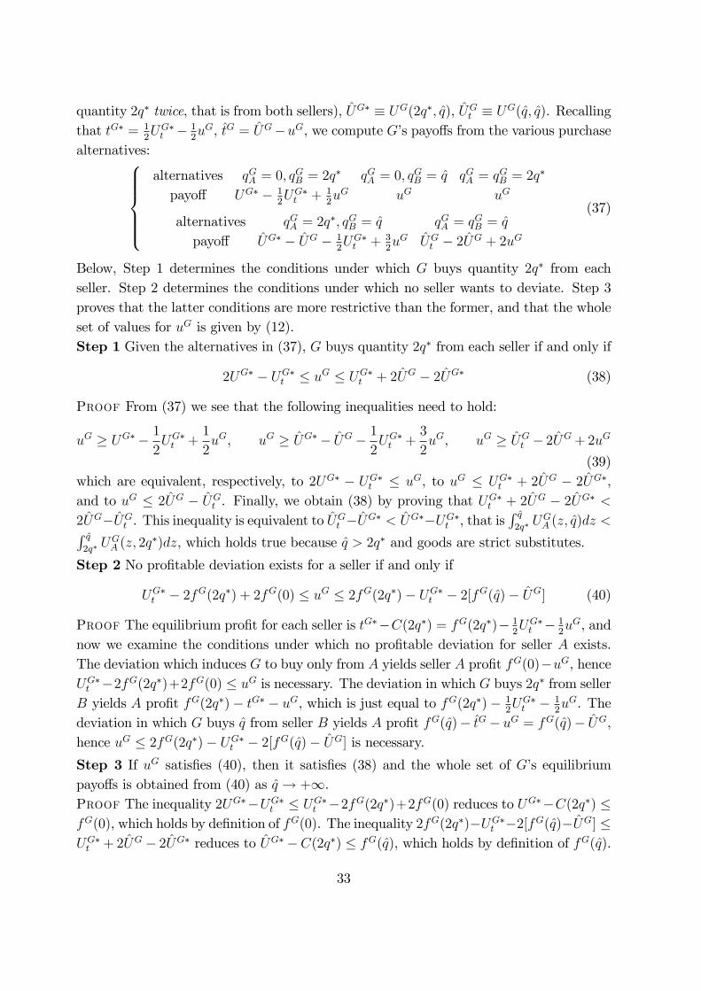
quantity 2q∗ twice, that is from both sellers), UG∗ ≡ UG(2q∗, q), UGt ≡ UG(q, q). Recallingthat tG∗ = 1

2UG∗t − 1

2uG, tG = UG−uG, we compute G’s payoffs from the various purchase

alternatives:alternatives qGA = 0, qGB = 2q∗ qGA = 0, qGB = q qGA = qGB = 2q∗

payoff UG∗ − 12UG∗t + 1

2uG uG uG

alternatives qGA = 2q∗, qGB = q qGA = qGB = q

payoff UG∗ − UG − 12UG∗t + 3

2uG UGt − 2UG + 2uG

(37)

Below, Step 1 determines the conditions under which G buys quantity 2q∗ from eachseller. Step 2 determines the conditions under which no seller wants to deviate. Step 3proves that the latter conditions are more restrictive than the former, and that the wholeset of values for uG is given by (12).Step 1 Given the alternatives in (37), G buys quantity 2q∗ from each seller if and only if

2UG∗ − UG∗t ≤ uG ≤ UG∗t + 2UG − 2UG∗ (38)

Proof From (37) we see that the following inequalities need to hold:

uG ≥ UG∗− 1

2UG∗t +

1

2uG, uG ≥ UG∗− UG− 1

2UG∗t +

3

2uG, uG ≥ UGt − 2UG + 2uG

(39)which are equivalent, respectively, to 2UG∗ − UG∗t ≤ uG, to uG ≤ UG∗t + 2UG − 2UG∗,and to uG ≤ 2UG − UGt . Finally, we obtain (38) by proving that UG∗t + 2UG − 2UG∗ <

2UG−UGt . This inequality is equivalent to UGt −UG∗ < UG∗−UG∗t , that is∫ q2q∗ U

GA (z, q)dz <∫ q

2q∗ UGA (z, 2q∗)dz, which holds true because q > 2q∗ and goods are strict substitutes.

Step 2 No profitable deviation exists for a seller if and only if

UG∗t − 2fG(2q∗) + 2fG(0) ≤ uG ≤ 2fG(2q∗)− UG∗t − 2[fG(q)− UG] (40)

Proof The equilibrium profit for each seller is tG∗−C(2q∗) = fG(2q∗)− 12UG∗t − 1

2uG, and

now we examine the conditions under which no profitable deviation for seller A exists.The deviation which induces G to buy only from A yields seller A profit fG(0)−uG, henceUG∗t −2fG(2q∗)+2fG(0) ≤ uG is necessary. The deviation in which G buys 2q∗ from sellerB yields A profit fG(2q∗)− tG∗ − uG, which is just equal to fG(2q∗)− 1

2UG∗t − 1

2uG. The

deviation in which G buys q from seller B yields A profit fG(q)− tG− uG = fG(q)− UG,hence uG ≤ 2fG(2q∗)− UG∗t − 2[fG(q)− UG] is necessary.

Step 3 If uG satisfies (40), then it satisfies (38) and the whole set of G’s equilibriumpayoffs is obtained from (40) as q → +∞.Proof The inequality 2UG∗−UG∗t ≤ UG∗t −2fG(2q∗)+2fG(0) reduces to UG∗−C(2q∗) ≤fG(0), which holds by definition of fG(0). The inequality 2fG(2q∗)−UG∗t −2[fG(q)−UG] ≤UG∗t + 2UG− 2UG∗ reduces to UG∗−C(2q∗) ≤ fG(q), which holds by definition of fG(q).

33

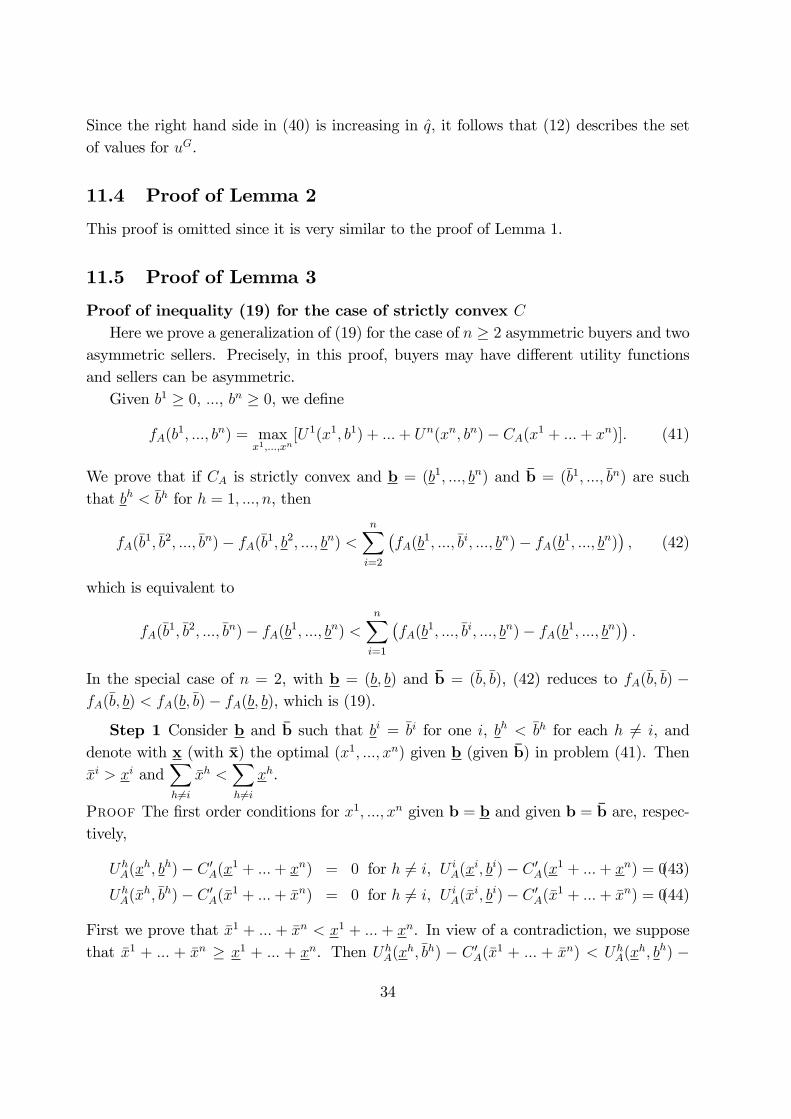
Since the right hand side in (40) is increasing in q, it follows that (12) describes the setof values for uG.

11.4 Proof of Lemma 2

This proof is omitted since it is very similar to the proof of Lemma 1.

11.5 Proof of Lemma 3

Proof of inequality (19) for the case of strictly convex CHere we prove a generalization of (19) for the case of n ≥ 2 asymmetric buyers and two

asymmetric sellers. Precisely, in this proof, buyers may have different utility functionsand sellers can be asymmetric.Given b1 ≥ 0, ..., bn ≥ 0, we define

fA(b1, ..., bn) = maxx1,...,xn

[U1(x1, b1) + ...+ Un(xn, bn)− CA(x1 + ...+ xn)]. (41)

We prove that if CA is strictly convex and b = (b1, ..., bn) and b = (b1, ..., bn) are suchthat bh < bh for h = 1, ..., n, then

fA(b1, b2, ..., bn)− fA(b1, b2, ..., bn) <n∑i=2

(fA(b1, ..., bi, ..., bn)− fA(b1, ..., bn)

), (42)

which is equivalent to

fA(b1, b2, ..., bn)− fA(b1, ..., bn) <n∑i=1

(fA(b1, ..., bi, ..., bn)− fA(b1, ..., bn)

).

In the special case of n = 2, with b = (b, b) and b = (b, b), (42) reduces to fA(b, b) −fA(b, b) < fA(b, b)− fA(b, b), which is (19).

Step 1 Consider b and b such that bi = bi for one i, bh < bh for each h 6= i, anddenote with x (with x) the optimal (x1, ..., xn) given b (given b) in problem (41). Thenxi > xi and

∑h6=i

xh <∑h6=i

xh.

Proof The first order conditions for x1, ..., xn given b = b and given b = b are, respec-tively,

UhA(xh, bh)− C ′A(x1 + ...+ xn) = 0 for h 6= i, U iA(xi, bi)− C ′A(x1 + ...+ xn) = 0(43)

UhA(xh, bh)− C ′A(x1 + ...+ xn) = 0 for h 6= i, U iA(xi, bi)− C ′A(x1 + ...+ xn) = 0(44)

First we prove that x1 + ... + xn < x1 + ... + xn. In view of a contradiction, we supposethat x1 + ... + xn ≥ x1 + ... + xn. Then UhA(xh, bh) − C ′A(x1 + ... + xn) < UhA(xh, bh) −

34

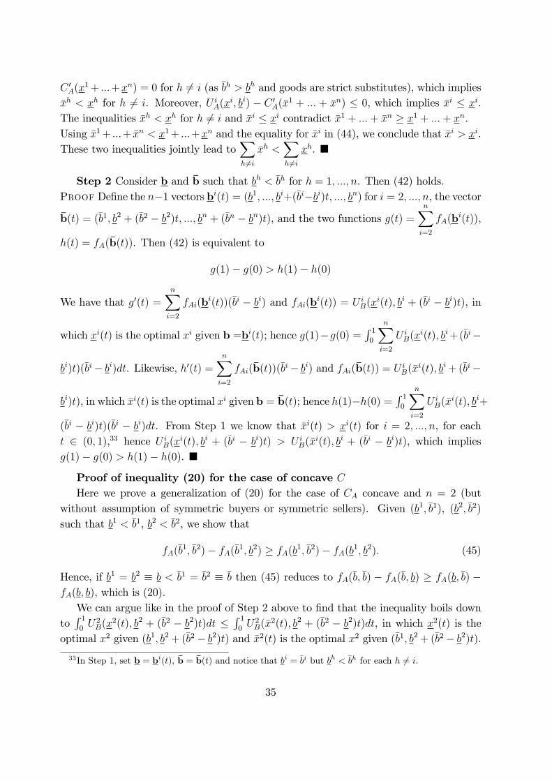
C ′A(x1+ ...+xn) = 0 for h 6= i (as bh > bh and goods are strict substitutes), which impliesxh < xh for h 6= i. Moreover, U iA(xi, bi) − C ′A(x1 + ... + xn) ≤ 0, which implies xi ≤ xi.The inequalities xh < xh for h 6= i and xi ≤ xi contradict x1 + ...+ xn ≥ x1 + ...+ xn.Using x1+ ...+ xn < x1+ ...+xn and the equality for xi in (44), we conclude that xi > xi.These two inequalities jointly lead to

∑h6=i

xh <∑h6=i

xh. �

Step 2 Consider b and b such that bh < bh for h = 1, ..., n. Then (42) holds.Proof Define the n−1 vectors bi(t) = (b1, ..., bi+(bi−bi)t, ..., bn) for i = 2, ..., n, the vector

b(t) = (b1, b2 + (b2 − b2)t, ..., bn + (bn − bn)t), and the two functions g(t) =n∑i=2

fA(bi(t)),

h(t) = fA(b(t)). Then (42) is equivalent to

g(1)− g(0) > h(1)− h(0)

We have that g′(t) =n∑i=2

fAi(bi(t))(bi − bi) and fAi(bi(t)) = U iB(xi(t), bi + (bi − bi)t), in

which xi(t) is the optimal xi given b =bi(t); hence g(1)−g(0) =∫ 10

n∑i=2

U iB(xi(t), bi+(bi−

bi)t)(bi− bi)dt. Likewise, h′(t) =n∑i=2

fAi(b(t))(bi− bi) and fAi(b(t)) = U iB(xi(t), bi + (bi−

bi)t), in which xi(t) is the optimal xi given b = b(t); hence h(1)−h(0) =∫ 10

n∑i=2

U iB(xi(t), bi+

(bi − bi)t)(bi − bi)dt. From Step 1 we know that xi(t) > xi(t) for i = 2, ..., n, for eacht ∈ (0, 1),33 hence U iB(xi(t), bi + (bi − bi)t) > U iB(xi(t), bi + (bi − bi)t), which impliesg(1)− g(0) > h(1)− h(0). �

Proof of inequality (20) for the case of concave CHere we prove a generalization of (20) for the case of CA concave and n = 2 (but

without assumption of symmetric buyers or symmetric sellers). Given (b1, b1), (b2, b2)

such that b1 < b1, b2 < b2, we show that

fA(b1, b2)− fA(b1, b2) ≥ fA(b1, b2)− fA(b1, b2). (45)

Hence, if b1 = b2 ≡ b < b1 = b2 ≡ b then (45) reduces to fA(b, b) − fA(b, b) ≥ fA(b, b) −fA(b, b), which is (20).We can argue like in the proof of Step 2 above to find that the inequality boils down

to∫ 10U2B(x2(t), b2 + (b2 − b2)t)dt ≤

∫ 10U2B(x2(t), b2 + (b2 − b2)t)dt, in which x2(t) is the

optimal x2 given (b1, b2 + (b2− b2)t) and x2(t) is the optimal x2 given (b1, b2 + (b2− b2)t).33In Step 1, set b = bi(t), b = b(t) and notice that bi = bi but bh < bh for each h 6= i.

35

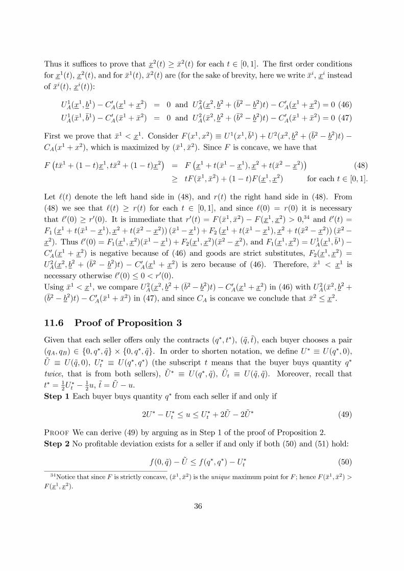
Thus it suffi ces to prove that x2(t) ≥ x2(t) for each t ∈ [0, 1]. The first order conditionsfor x1(t), x2(t), and for x1(t), x2(t) are (for the sake of brevity, here we write xi, xi insteadof xi(t), xi(t)):

U1A(x1, b1)− C ′A(x1 + x2) = 0 and U2A(x2, b2 + (b2 − b2)t)− C ′A(x1 + x2) = 0 (46)

U1A(x1, b1)− C ′A(x1 + x2) = 0 and U2A(x2, b2 + (b2 − b2)t)− C ′A(x1 + x2) = 0 (47)

First we prove that x1 < x1. Consider F (x1, x2) ≡ U1(x1, b1) + U2(x2, b2 + (b2 − b2)t) −CA(x1 + x2), which is maximized by (x1, x2). Since F is concave, we have that

F(tx1 + (1− t)x1, tx2 + (1− t)x2

)= F

(x1 + t(x1 − x1), x2 + t(x2 − x2)

)(48)

≥ tF (x1, x2) + (1− t)F (x1, x2) for each t ∈ [0, 1].

Let `(t) denote the left hand side in (48), and r(t) the right hand side in (48). From(48) we see that `(t) ≥ r(t) for each t ∈ [0, 1], and since `(0) = r(0) it is necessarythat `′(0) ≥ r′(0). It is immediate that r′(t) = F (x1, x2) − F (x1, x2) > 0,34 and `′(t) =

F1 (x1 + t(x1 − x1), x2 + t(x2 − x2)) (x1− x1) +F2 (x1 + t(x1 − x1), x2 + t(x2 − x2)) (x2−x2). Thus `′(0) = F1(x

1, x2)(x1 − x1) + F2(x1, x2)(x2 − x2), and F1(x1, x2) = U1A(x1, b1)−

C ′A(x1 + x2) is negative because of (46) and goods are strict substitutes, F2(x1, x2) =

U2A(x2, b2 + (b2 − b2)t) − C ′A(x1 + x2) is zero because of (46). Therefore, x1 < x1 isnecessary otherwise `′(0) ≤ 0 < r′(0).Using x1 < x1, we compare U2A(x2, b2 + (b2 − b2)t)−C ′A(x1 + x2) in (46) with U2A(x2, b2 +

(b2 − b2)t)− C ′A(x1 + x2) in (47), and since CA is concave we conclude that x2 ≤ x2.

11.6 Proof of Proposition 3

Given that each seller offers only the contracts (q∗, t∗), (q, t), each buyer chooses a pair(qA, qB) ∈ {0, q∗, q} × {0, q∗, q}. In order to shorten notation, we define U∗ ≡ U(q∗, 0),U ≡ U(q, 0), U∗t ≡ U(q∗, q∗) (the subscript t means that the buyer buys quantity q∗

twice, that is from both sellers), U∗ ≡ U(q∗, q), Ut ≡ U(q, q). Moreover, recall thatt∗ = 1

2U∗t − 1

2u, t = U − u.

Step 1 Each buyer buys quantity q∗ from each seller if and only if

2U∗ − U∗t ≤ u ≤ U∗t + 2U − 2U∗ (49)

Proof We can derive (49) by arguing as in Step 1 of the proof of Proposition 2.Step 2 No profitable deviation exists for a seller if and only if both (50) and (51) hold:

f(0, q)− U ≤ f(q∗, q∗)− U∗t (50)

34Notice that since F is strictly concave, (x1, x2) is the unique maximum point for F ; hence F (x1, x2) >

F (x1, x2).

36

max{U∗t − 2f(q∗, q∗) + 2f(0, q∗), U∗t − f(q∗, q∗) + f(0, 0)} ≤ u

andu ≤ min{2f(q∗, q∗)− U∗t − 2[f(q∗, q)− U ], f(q∗, q∗)− U∗t − [f(q, q)− 2U ]}

(51)

Proof For each seller, the equilibrium profit is π∗ ≡ 2t∗ − C∗ = f(q∗, q∗) − U∗t − u, inwhich C∗ ≡ C(2q∗). We consider the possible deviations of seller A.(i) The deviation which induces both buyers to buy only from A yields A the profitf(0, 0)− 2u, and the inequality f(0, 0)− 2u ≤ π∗ reduces to U∗t − f(q∗, q∗) + f(0, 0) ≤ u.(ii) The deviation which induces buyer 1 to buy only from A and buyer 2 to buy q∗ fromB yields A the profit f(0, q∗)− t∗− 2u, and the inequality f(0, q∗)− t∗− 2u ≤ π∗ reducesto U∗t − 2f(q∗, q∗) + 2f(0, q∗) ≤ u.(iii) The deviation which induces buyer 1 to buy only from A and buyer 2 to buy q fromB yields A the profit f(0, q)− t− 2u, and the inequality f(0, q)− t− 2u ≤ π∗ reduces to(50).(iv) The deviation which induces both buyers to buy q∗ from B yields A the profitf(q∗, q∗)− 2t∗ − 2u = f(q∗, q∗)− U∗t − u, which is just the equilibrium profit.(v) The deviation which induces buyer 1 to buy q∗ from B and buyer 2 to buy q from B

yields A the profit f(q∗, q) − t∗ − t − 2u, and the inequality f(q∗, q) − t∗ − t − 2u ≤ π∗

reduces to u ≤ 2f(q∗, q∗)− U∗t − 2[f(q∗, q)− U ].(vi) The deviation which induces both buyers to buy q from B yields A the profit f(q, q)−2t−2u, and the inequality f(q, q)−2t−2u ≤ π∗ reduces to u ≤ f(q∗, q∗)−U∗t −[f(q, q)−2U ].The inequalities obtained from (i)-(ii) and (v)-(vi) are summarized by (51).

Step 3 If u satisfies (51), then it satisfies (49).Proof The inequality 2U∗ − U∗t ≤ U∗t − f(q∗, q∗) + f(0, 0) is equivalent to 2U∗ − C∗ ≤f(0, 0), which holds by definition of f(0, 0). The inequality f(q∗, q∗)−U∗t −[f(q, q)−2U ] ≤U∗t + 2U − 2U∗ is equivalent to 2U∗ − C∗ ≤ f(q, q), which holds by definition of f(q, q).

Step 4 If C is strictly convex, then no profitable deviation exists for a seller if and onlyif (50) and (52) both hold, with

U∗t − 2f(q∗, q∗) + 2f(0, q∗) ≤ u ≤ 2f(q∗, q∗)− U∗t − 2[f(q∗, q)− U ] (52)

If C is concave, then no profitable deviation exists for a seller if and only if (50) and (53)both hold, with

U∗t − f(q∗, q∗) + f(0, 0) ≤ u ≤ f(q∗, q∗)− U∗t − [f(q, q)− 2U ] (53)

Proof We prove that (51) reduces to (52) if C is strictly convex, and that (51) reducesto (53) if C is concave.The inequality U∗t − f(q∗, q∗) + f(0, 0) < U∗t − 2f(q∗, q∗) + 2f(0, q∗) is equivalent tof(q∗, q∗) − f(q∗, 0) < f(0, q∗) − f(0, 0), which holds if C is strictly convex, by (19).

37

Conversely, if C is concave then (20) applies and it follows that U∗t − f(q∗, q∗) + f(0, 0) ≥U∗t − 2f(q∗, q∗) + 2f(0, q∗) holds. The inequality 2f(q∗, q∗) − U∗t − 2[f(q∗, q) − U ] <

f(q∗, q∗) − U∗t − [f(q, q) − 2U ] is equivalent to f(q, q) − f(q, q∗) < f(q∗, q) − f(q∗, q∗),which holds if C is strictly convex, by (19). Conversely, if C is concave then (20) appliesand it follows that 2f(q∗, q∗)− U∗t − 2[f(q∗, q)− U ] ≥ f(q∗, q∗)− U∗t − [f(q, q)− 2U ].

Step 5 Increasing q relaxes (50), (52), and (53).Proof In the left hand side in (50), f(0, q)−U = maxx,y[U(x, 0)+

∫ y0UA(z, q)dz−C(x+y)]

is decreasing in q since goods are substitutes. The same property implies that the righthand side in (52), 2U − 2f(q∗, q) = −2 maxx,y[U(x, q∗) +

∫ y0UA(z, q)dz −C(x+ y)], is in-

creasing in q as well as the right hand side in (53), 2U−f(q, q) = −maxx,y[∫ x0UA(z, q)dz+∫ y

0UA(z, q)dz − C(x+ y)].

Step 6 Inequality (50) holds if q is suffi ciently large, and the whole set of values for u isobtained from (52) and (53) as q → +∞.Proof The left hand side in (50) is equal to maxx,y[U(x, 0) +

∫ y0UA(z, q)dz −C(x+ y)],

whereas the right hand side in (50) is equal to U∗t − C∗ = maxx,y (U(x, y)− C(x+ y)).We prove that limq→+∞[U(x, 0) +

∫ y0UA(z, q)dz] < U(x, y), which implies that (50) holds

for a large q. Precisely, the previous inequality is equivalent to limq→+∞∫ y0UA(z, q)dz <∫ y

0UB(x, z)dz =

∫ y0UA(z, x)dz (since U is symmetric), and the latter inequality holds

since goods are strict substitutes.

11.7 Proof of Proposition 5

For j = A,B, let V Gj ≡ maxq1j ,...,qnj (U1(q1j , 0) + ...+Un(qnj , 0)−Cj(q1j + ...+ qnj )). Then in

each equilibrium under no group we have πA + u1 + ...+ un ≥ V GA because we can argue

as when n = 2 (see the argument just after Proposition 2, and notice that this argumentdoes not depend on whether or not a group is formed): if πA + u1 + ... + un < V G

A , thenseller A can deviate by offering to the buyers a suitable trade in which each buyer buysonly from A, and their joint payoffs increase to V G

A .Hence, we have πB ≤ V G

AB − V GA and πA ≤ V G

AB − V GB , which implies u

1 + ... + un ≥V GA +V G

B −V GAB, where V

GA +V G

B −V GAB is just the total payoff of the buyers in the sell-out

equilibrium under buyer group.Now we prove that without group, there exists no equilibrium satisfying u1+ ...+un =

V GA + V G

B − V GAB, hence u

1 + ... + un > V GA + V G

B − V GAB in each equilibrium. We argue

by contradiction and suppose that an equilibrium exists such that u1 + ... + un = V GA +

V GB − V G

AB. Then πA + πB = 2V G

AB − V GA − V G

B . This together with πA ≤ V G

AB − V GB and

πB ≤ V GAB − V G

A implies πA = V GAB − V G

B and πB = V GAB − V G

A .Then we suppose that CA (to fix the ideas) is strictly convex, and consider the de-

viation of seller A with bi = qi∗B for one i, bh = 0 for h 6= i. This yields A the profit

38

fA(0, ..., qi∗B , ..., 0) − ti∗B − (V GA + V G

B − V GAB),35 hence this deviation is unprofitable if and

only if fA(0, ..., qi∗B , ..., 0)−V GA ≤ ti∗B . The existence of no profitable deviation for A requires

that this inequality holds for i = 1, ..., n. Hence, we have

n∑i=1

fA(0, ..., qi∗B , ..., 0)− nV GA ≤ t1∗B + ...+ tn∗B . (54)

Then notice that πB = V GAB−V G

A is equivalent to t1∗B + ...+ tn∗B = V GAB−V G

A +CB(q1∗B + ...+

qn∗B ). In addition, we use (54), V GA = fA(0, ..., 0), V G

AB+CB(q1∗B + ...+qn∗B ) = fA(q1∗B , ..., qn∗B )

to obtain the inequality

n∑i=2

(fA(0, ..., qi∗B , ..., 0)− fA(0, ..., 0)

)≤ fA(q1∗B , ..., q

n∗B )− fA(q1∗B , ..., 0). (55)

Finally, we use (42) to show that (55) cannot hold: setting bi = 0, bi = qi∗B for i = 1, ..., n

in (42) yields the opposite of (55).

35The function fA is defined in (41).

39